BAEN 673

Biological and Agricultural Engineering Department

Texas A&M University

ArcSWAT / ArcGIS 10.1

Exercise 4: Kings Creek

Note: A personal flash drive is required. Create a folder named Ex4 on the flash drive for the

SWAT simulations. Copy the Exercise4_files.zip file to the Ex4 folder and extract all of the files.

Explanation: All the necessary files have already been downloaded and have been given

to you in the “Exercise4_files”. Some files required a re-projection, but that has also

already been done for you. The specific files you will need to use are “DEM”,

“Landuse_clip”, “StreamGageEvent_Project” (in the StreamGageEvent folder),

“nhdflowline_Project.shp” (in NHDLines Hydrography folder), and

“Subbasin_Project.shp” (in NHDLines HydrologicUnits folder).

For you to obtain hydrography dataset go to http://www.horizon-

systems.com/NHDPlus/NHDPlusV1_data.php (The resolution of the dataset is 30 m * 30

m) click TEXAS GULF (12) (we will use Hydrologic region 12a) read the

Download instructions download the DEM Region 12, Version 01_01, Elevation

Unit a download the flow lines Region 12, Version 01_01, National Hydrography

Dataset download the gauging station data Region 12, Version 01_01, Stream

Gage Event Extract all of the files to your working folder Ex4

Getting Started

1. Start ArcMap New Maps Blank Map Ok Customize Extensions check

Spatial Analyst / SWAT Project Manager / SWAT Watershed Delineator

***Make sure to save your files on a flash drive***

Explanation: Create an ArcMap project file using the ArcSWAT extension of ArcGIS

10.1 that will link GIS databases with the ArcSWAT hydrologic model.

Create new SWAT project / Setup working directory / Setup Geodatabases

1. SWAT Project Setup New SWAT Project Save current document? No Project

Setup dialog box appears Project Directory select folder icon connect to folder

navigate to the flash drive Ok select the Ex4 folder

(***single click***) Ok SWAT Project Geodatabase change the name to

Ex4Output.mdb (Note: You name this file anything but it must have a .mdb extension – it will go

in the Project Directory) Raster Storage leave the name RasterStore.mdb (it will go in the

Project Directory) SWAT Parameter Geodatabase leave the default path

G:\Ex4\SWAT2012.mdb Ok wait patiently Project setup is done Ok

Explanation: The Project Directory is where all of the project files will be stored.

Data preparation- DEM, Landuse Dataset, Soil Dataset, and Weather Dataset are required.

1. Start here add data add the DEM by navigating in the Ex4\Exercise4_files folder

highlight DEM Add Create pyramids for DEM No

Note: You should add DEM data to ArcGIS first!!! When you add data layers in ArcGIS, the

coordinate system of the data layers will be the same as the first added data layer.

2. Add data add the NHD Flow line by navigating in the Ex4\Exercise4_files folder

NHDlines Hydrography folder nhdflowline.shp Add

3. Add data add the Stream Gauge locations by navigating in the Exercise4_files folder

StreamGaugeEvent folder highlight StreamGaugeEvent.shp Add

4. Add data add the subbasin file by navigating in the Exercise4_files folder

NDHLines folder HydrologicUnits folder highlight Subbasin_project.shp Add

5. Under Layers (left hand side) click the right mouse button on the Subbasin_project layer

open attribute table click the Table Options icon Select by Attributes double

click “HUC_8” click “=” click Get Unique Values find and double click “12030107”

make sure the text above the box reads SELECT * FROM Subbasin_Project WHERE:

“HUC_8” = ‘12030107’ Apply Close window Under Layers (left hand side) right

click on the Subbasin_Project layer click Data click Export Data under Output feature

class: select the folder icon navigate to the Ex4 folder in the Name: box change the

name to Cedar.shp in the Save as type: box change to Shapefile Save Ok

Yes close the Table

6. Under Layers (left hand side) Right click on Subbasin_project remove

Note: This will focus on the Cedar watershed.

3. Extract stream gauging stations click on Geoprocessing from the toolbar single-click

Clip Input Features box click the down arrow click StreamGageEvent.shp Clip

Features box click the down arrow click Cedar Output Feature Class box click the

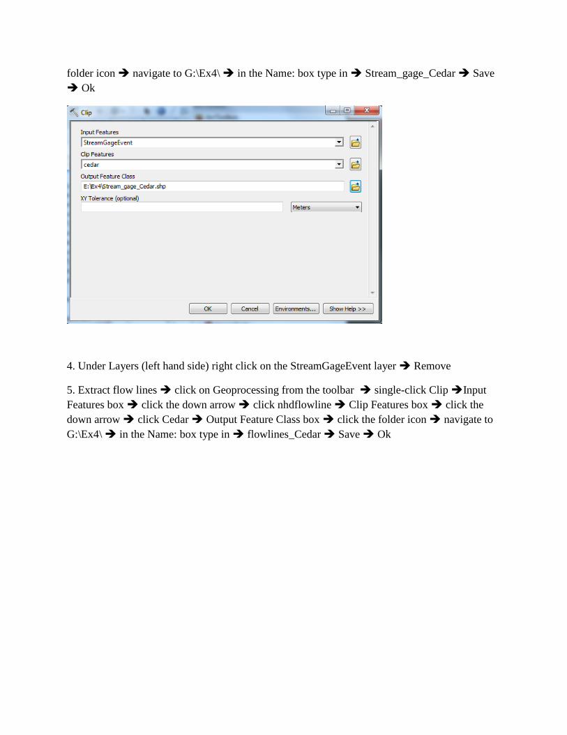
folder icon navigate to G:\Ex4\ in the Name: box type in Stream_gage_Cedar Save

Ok

4. Under Layers (left hand side) right click on the StreamGageEvent layer Remove

5. Extract flow lines click on Geoprocessing from the toolbar single-click Clip Input

Features box click the down arrow click nhdflowline Clip Features box click the

down arrow click Cedar Output Feature Class box click the folder icon navigate to

G:\Ex4\ in the Name: box type in flowlines_Cedar Save Ok

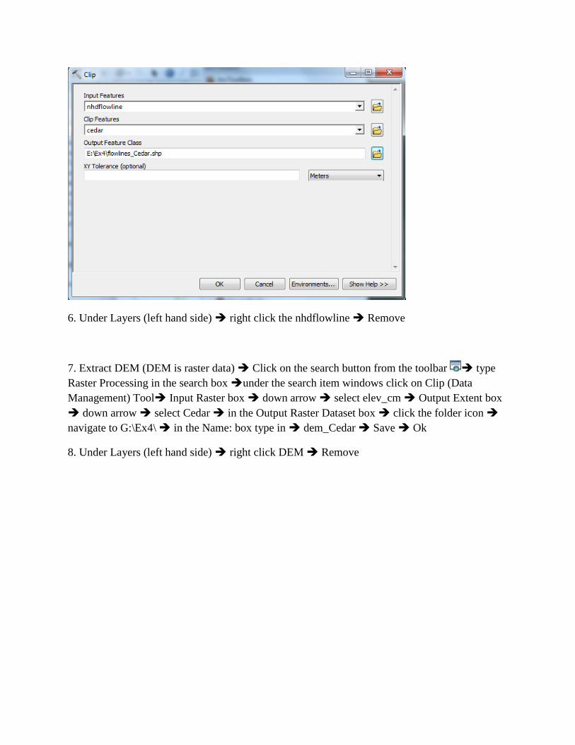
6. Under Layers (left hand side) right click the nhdflowline Remove

7. Extract DEM (DEM is raster data) Click on the search button from the toolbar type

Raster Processing in the search box under the search item windows click on Clip (Data

Management) Tool Input Raster box down arrow select elev_cm Output Extent box

down arrow select Cedar in the Output Raster Dataset box click the folder icon

navigate to G:\Ex4\ in the Name: box type in dem_Cedar Save Ok

8. Under Layers (left hand side) right click DEM Remove

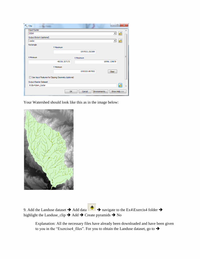
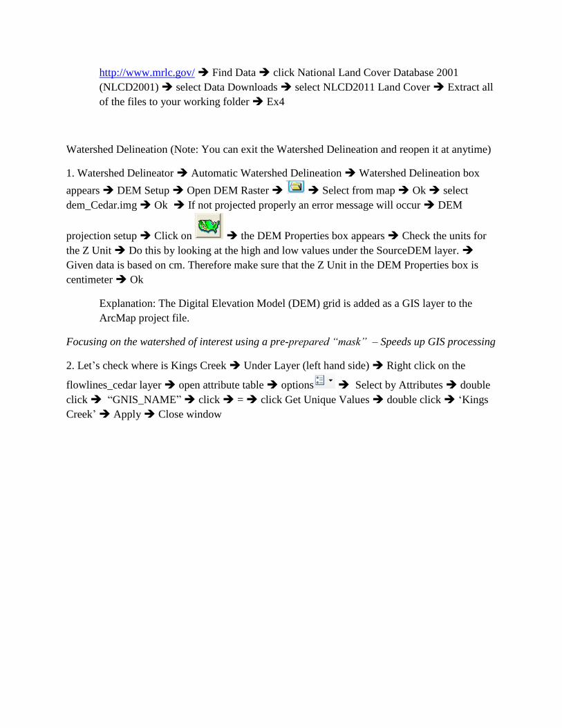
Your Watershed should look like this as in the image below:

9. Add the Landuse dataset Add data navigate to the Ex4\Exercis4 folder

highlight the Landuse_clip Add Create pyramids No

Explanation: All the necessary files have already been downloaded and have been given

to you in the “Exercise4_files”. For you to obtain the Landuse dataset, go to

http://www.mrlc.gov/ Find Data click National Land Cover Database 2001

(NLCD2001) select Data Downloads select NLCD2011 Land Cover Extract all

of the files to your working folder Ex4

Watershed Delineation (Note: You can exit the Watershed Delineation and reopen it at anytime)

1. Watershed Delineator Automatic Watershed Delineation Watershed Delineation box

appears DEM Setup Open DEM Raster Select from map Ok select

dem_Cedar.img Ok If not projected properly an error message will occur DEM

projection setup Click on the DEM Properties box appears Check the units for

the Z Unit Do this by looking at the high and low values under the SourceDEM layer.

Given data is based on cm. Therefore make sure that the Z Unit in the DEM Properties box is

centimeter Ok

Explanation: The Digital Elevation Model (DEM) grid is added as a GIS layer to the

ArcMap project file.

Focusing on the watershed of interest using a pre-prepared “mask” – Speeds up GIS processing

2. Let’s check where is Kings Creek Under Layer (left hand side) Right click on the

flowlines_cedar layer open attribute table options Select by Attributes double

click “GNIS_NAME” click = click Get Unique Values double click ‘Kings

Creek’ Apply Close window

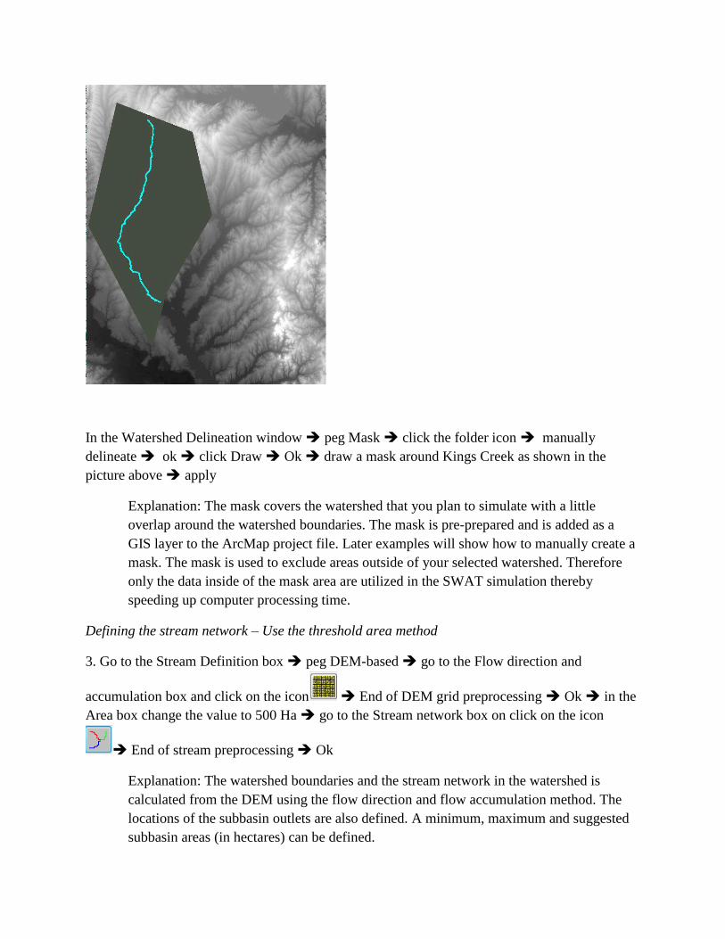
In the Watershed Delineation window peg Mask click the folder icon manually

delineate ok click Draw Ok draw a mask around Kings Creek as shown in the

picture above apply

Explanation: The mask covers the watershed that you plan to simulate with a little

overlap around the watershed boundaries. The mask is pre-prepared and is added as a

GIS layer to the ArcMap project file. Later examples will show how to manually create a

mask. The mask is used to exclude areas outside of your selected watershed. Therefore

only the data inside of the mask area are utilized in the SWAT simulation thereby

speeding up computer processing time.

Defining the stream network – Use the threshold area method

3. Go to the Stream Definition box peg DEM-based go to the Flow direction and

accumulation box and click on the icon End of DEM grid preprocessing Ok in the

Area box change the value to 500 Ha go to the Stream network box on click on the icon

End of stream preprocessing Ok

Explanation: The watershed boundaries and the stream network in the watershed is

calculated from the DEM using the flow direction and flow accumulation method. The

locations of the subbasin outlets are also defined. A minimum, maximum and suggested

subbasin areas (in hectares) can be defined.

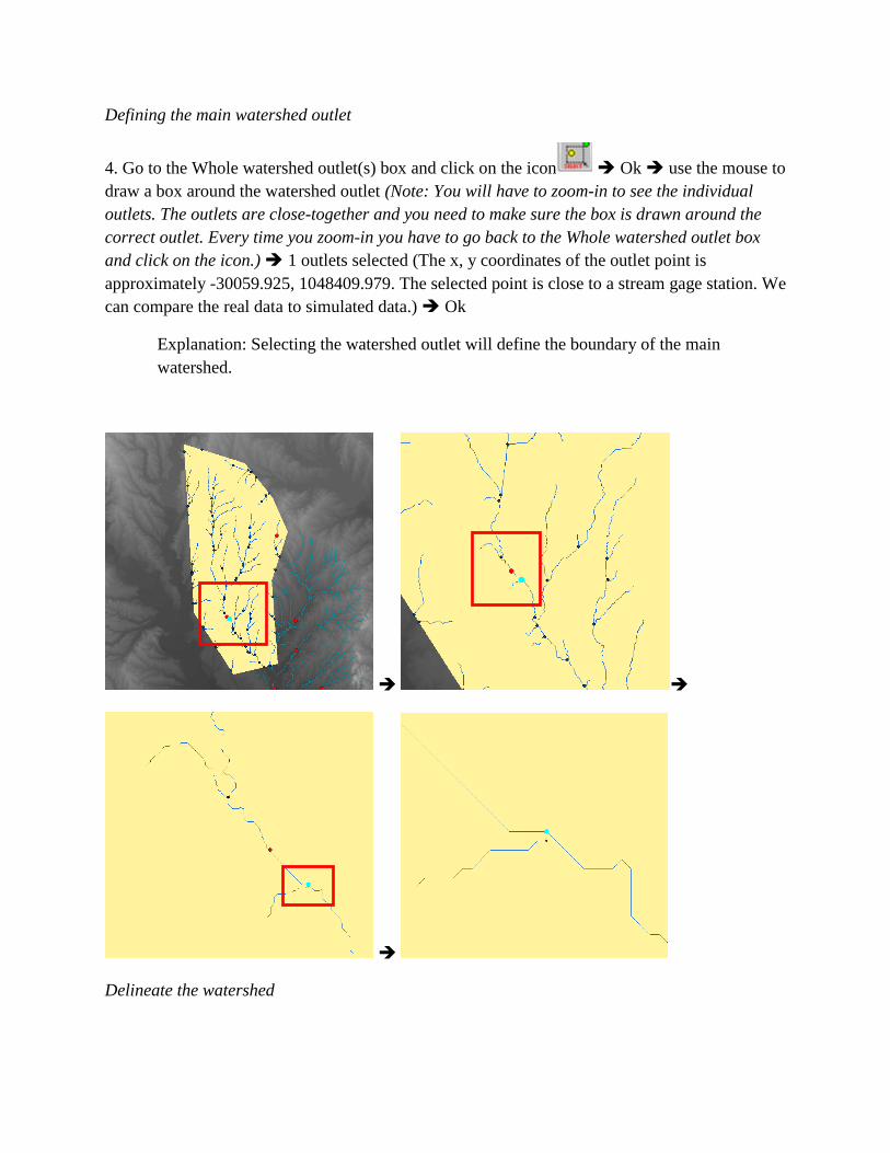
Defining the main watershed outlet

4. Go to the Whole watershed outlet(s) box and click on the icon Ok use the mouse to

draw a box around the watershed outlet (Note: You will have to zoom-in to see the individual

outlets. The outlets are close-together and you need to make sure the box is drawn around the

correct outlet. Every time you zoom-in you have to go back to the Whole watershed outlet box

and click on the icon.) 1 outlets selected (The x, y coordinates of the outlet point is

approximately -30059.925, 1048409.979. The selected point is close to a stream gage station. We

can compare the real data to simulated data.) Ok

Explanation: Selecting the watershed outlet will define the boundary of the main

watershed.

Delineate the watershed

5. Go to the Delineate watershed box and click on the icon Watershed delineation is done

Ok

Explanation: After this step the delineated watershed with all subbasins will be added as a

GIS layer to the ArcMap project file.

Calculate the subbasin parameters

6. Go to the calculate subbasin parameters box and click on the icon (wait patiently!)

Subbasin parameter calculation successfully done Ok Exit from the Watershed

Delineation box

Explanation: This function calculates basic watershed and subbasin characteristics from

the DEM. A Topographic Report can be opened by going to the Watershed Delineator

tab Watershed Reports Topographic Report Ok. Each subbasin is given a

unique ID number.

Defining the Land Use

1. HRU Analysis Land Use / Soils / Slope Definition Land Use Data tab the Land Use

Grid box and click on the open file folder icon peg Load Land Use dataset(s) from map

Open peg Grid select Landuse_clip Open Ok

(If you have a projection error message, follow the optional procedure (***), if not skip

it.)

*** Optional (if you have an error message associated with a projection problem.)

Click on search button on the toolbar type in project raster in the search box

click on Project Rater (Data Management) Project Raster (see below: input raster is

your clipped landuse raster data. Save as landuse_Clip_Proj.img output coordinate

system click layers NAD_1983_Albers select dem_cedar.shp in your

project folder

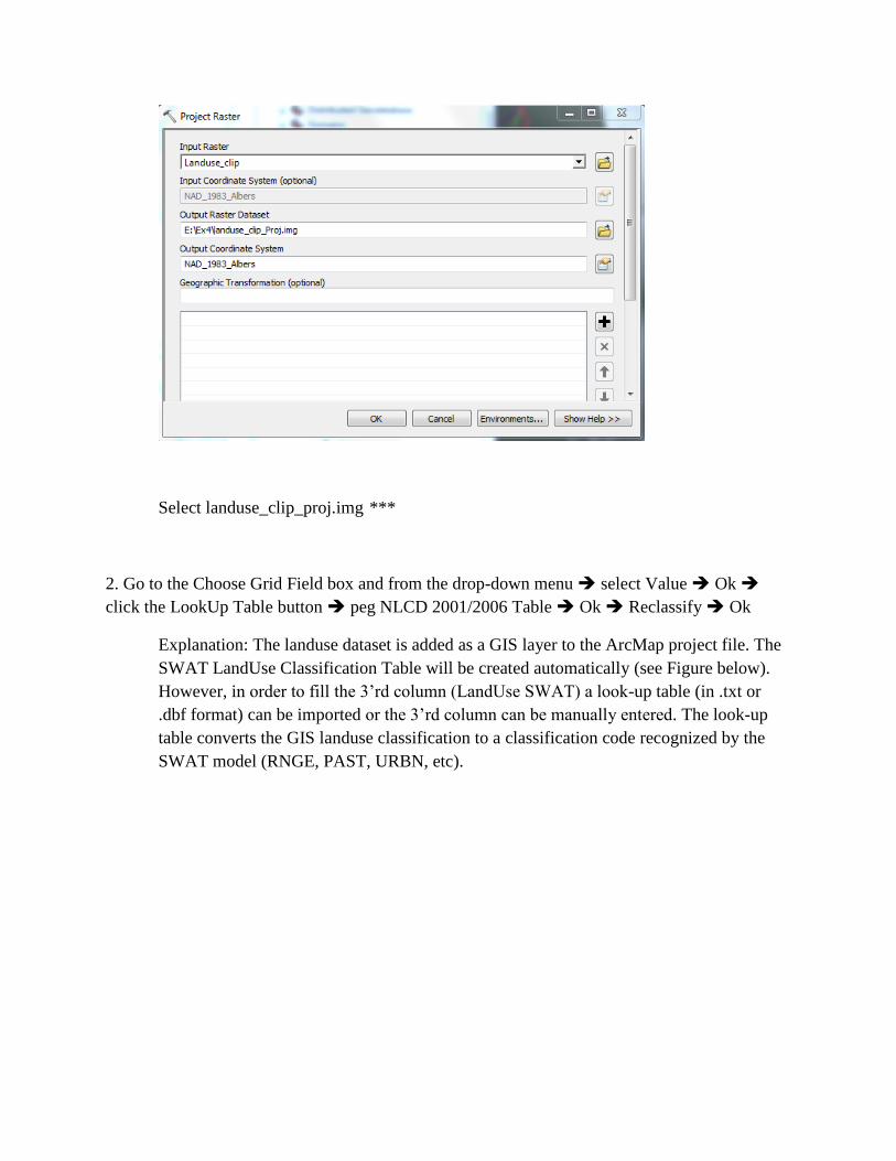
Select landuse_clip_proj.img ***

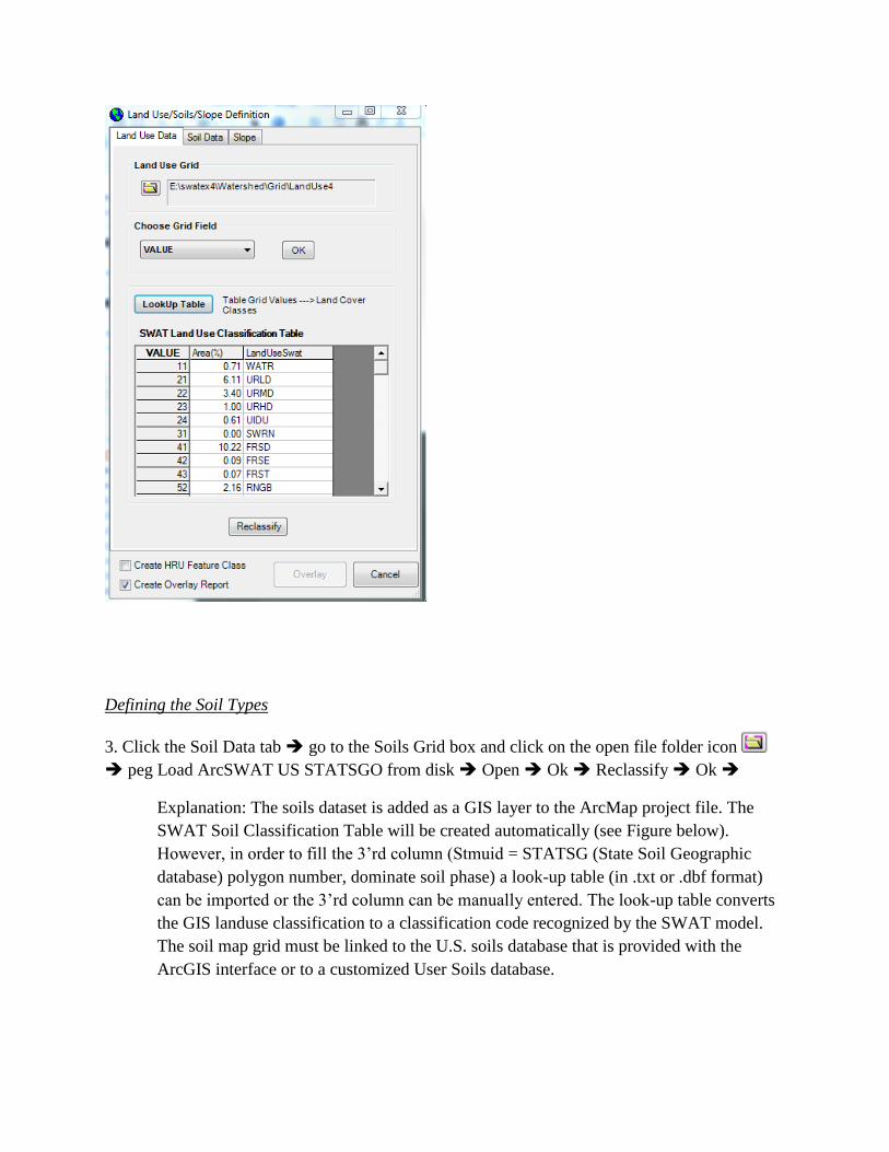
2. Go to the Choose Grid Field box and from the drop-down menu select Value Ok

click the LookUp Table button peg NLCD 2001/2006 Table Ok Reclassify Ok

Explanation: The landuse dataset is added as a GIS layer to the ArcMap project file. The

SWAT LandUse Classification Table will be created automatically (see Figure below).

However, in order to fill the 3’rd column (LandUse SWAT) a look-up table (in .txt or

.dbf format) can be imported or the 3’rd column can be manually entered. The look-up

table converts the GIS landuse classification to a classification code recognized by the

SWAT model (RNGE, PAST, URBN, etc).

Defining the Soil Types

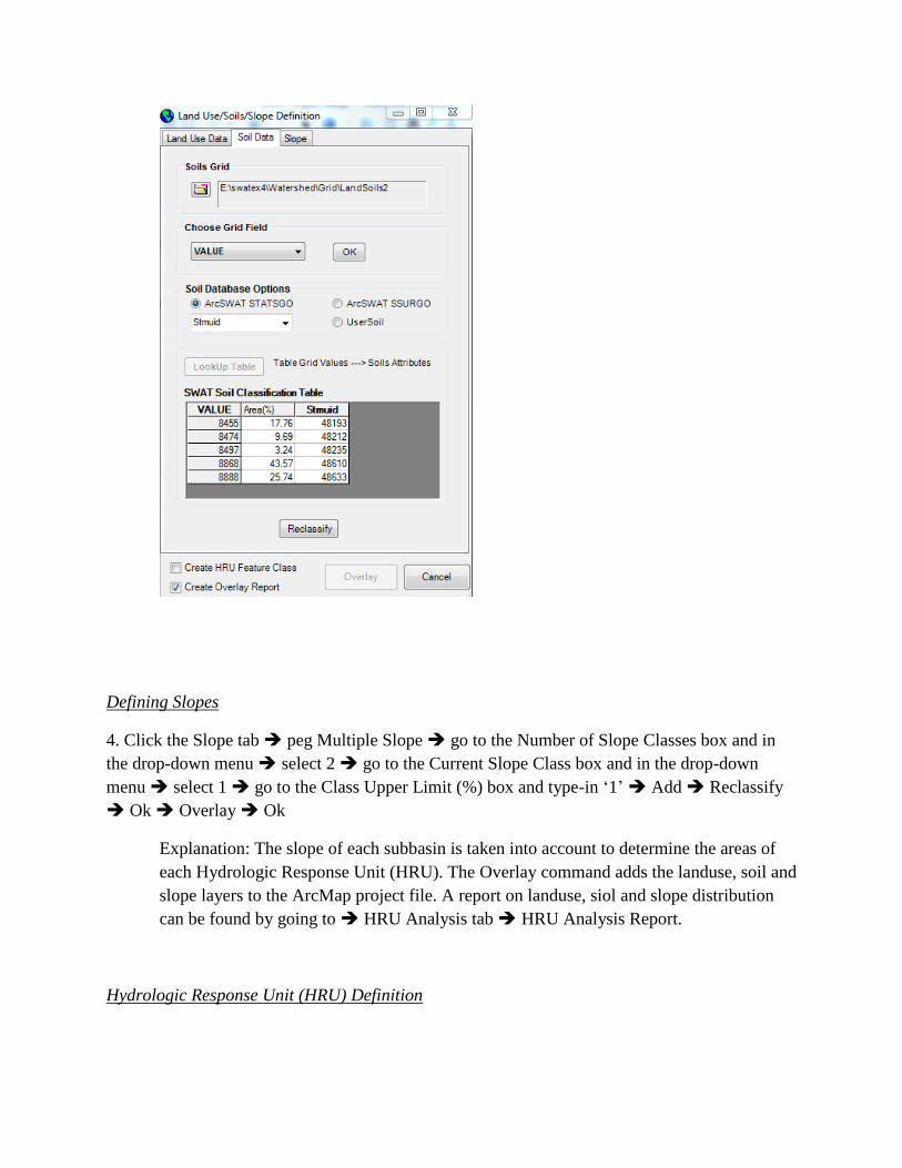
3. Click the Soil Data tab go to the Soils Grid box and click on the open file folder icon

peg Load ArcSWAT US STATSGO from disk Open Ok Reclassify Ok

Explanation: The soils dataset is added as a GIS layer to the ArcMap project file. The

SWAT Soil Classification Table will be created automatically (see Figure below).

However, in order to fill the 3’rd column (Stmuid = STATSG (State Soil Geographic

database) polygon number, dominate soil phase) a look-up table (in .txt or .dbf format)

can be imported or the 3’rd column can be manually entered. The look-up table converts

the GIS landuse classification to a classification code recognized by the SWAT model.

The soil map grid must be linked to the U.S. soils database that is provided with the

ArcGIS interface or to a customized User Soils database.

Defining Slopes

4. Click the Slope tab peg Multiple Slope go to the Number of Slope Classes box and in

the drop-down menu select 2 go to the Current Slope Class box and in the drop-down

menu select 1 go to the Class Upper Limit (%) box and type-in ‘1’ Add Reclassify

Ok Overlay Ok

Explanation: The slope of each subbasin is taken into account to determine the areas of

each Hydrologic Response Unit (HRU). The Overlay command adds the landuse, soil and

slope layers to the ArcMap project file. A report on landuse, siol and slope distribution

can be found by going to HRU Analysis tab HRU Analysis Report.

Hydrologic Response Unit (HRU) Definition

1. HRU Analysis HRU Definition HRU Thresholds peg Multiple HRUs go to the

Land use percentage (%) over subbasin area box and type-in 10% go to the Soil class

percentage (%) over land use area box and type-in 10% go to the Slope class percentage (%)

over soil area box and type-in 10% Create HRUs Ok

Explanation: The distribution of HRUs within each subbasin is calculated based on the

landuse, soil and slope layers. The interface allows the user to specify criteria for landuse,

soil and slope to be used in determining the HRU distribution. One on more unique

landuse, soil and slope combinations can be created for each subbasin. Runoff is

simulated separately for each HRU and routed to the stream channel in the subbasin.

Input the Weather Data

Search and find the weather stations and database Go to http://www.ncdc.noaa.gov/cdo-

web/search

For Weather Observation Type/Dataset Choose Daily Summaries

For Select Date Range Beginning: Jan. 1, 1999 End: Dec. 31, 2000

For Search For Hydrologic Cataloging Unit

For Enter a Search Term 12030107

Then press Search

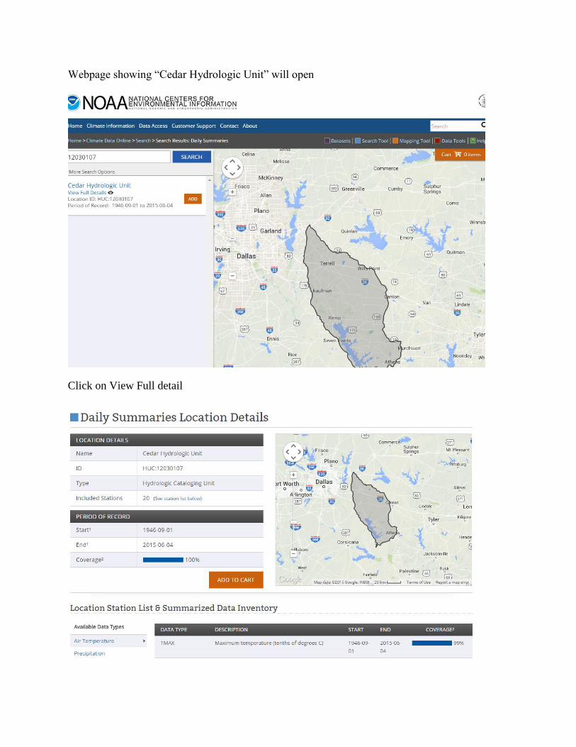
Webpage showing “Cedar Hydrologic Unit” will open

Click on View Full detail

Click on “See station list below” Click the add button in front of “Kaufman 3 SE, TX US”

and “Terrel Municipal Airport, TX US”

Note: For Terrel Municipal Airport, TX US station you will have to click next page button

at the bottom of the screen

On the top right corner Click on Cart click View All items

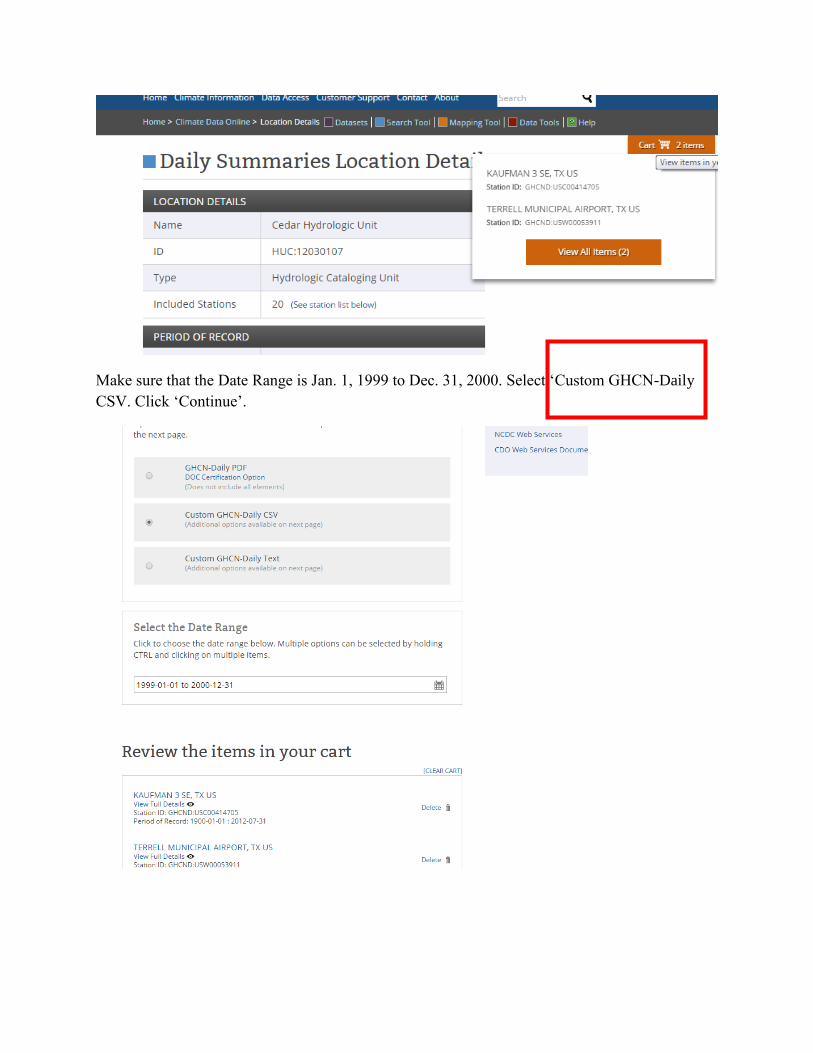
Make sure that the Date Range is Jan. 1, 1999 to Dec. 31, 2000. Select ‘Custom GHCN-Daily

CSV. Click ‘Continue’.

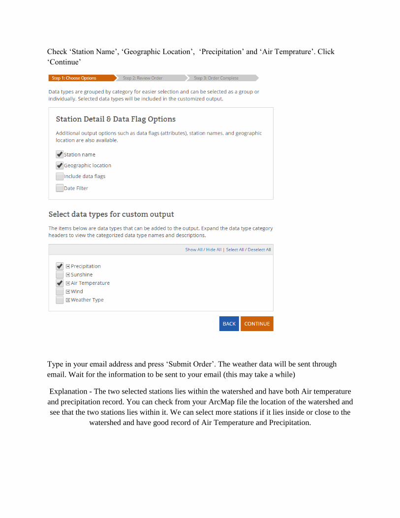
Check ‘Station Name’, ‘Geographic Location’, ‘Precipitation’ and ‘Air Temprature’. Click

‘Continue’

Type in your email address and press ‘Submit Order’. The weather data will be sent through

email. Wait for the information to be sent to your email (this may take a while)

Explanation - The two selected stations lies within the watershed and have both Air temperature

and precipitation record. You can check from your ArcMap file the location of the watershed and

see that the two stations lies within it. We can select more stations if it lies inside or close to the

watershed and have good record of Air Temperature and Precipitation.

The weather data format will need to be changed for input into SWAT. Six files are needed, 1)

the station information files of both stations and, 2) the precipitation data files for both the

stations and the Air temperature data files for both the stations. Remember that the units of the

downloaded data are English units and that the input data for SWAT must be in SI units.

PCP_CEDAR.txt and TMP_CEDAR.txt includes stations information such as ID(different for

different stations used) Name (this name should match to your data file name.), coordinate

systems (Latitude and Longitude, not Xpr and Ypr) and elevation (m).

pcp_terrel.txt and pcp_kaufman.txt includes date and precipitation (mm), and tmp_emory.txt

and tmp_kaufman. txt includes date and air temperature (°C).

Note: .txt is just an extension don’t save your file with naming .txt after the name, it will already

be made in .txt format if you made it in notepad.

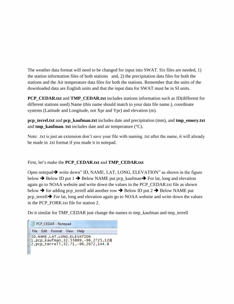
First, let’s make the PCP_CEDAR.txt and TMP_CEDAR.txt

Open notepad write down” ID, NAME, LAT, LONG, ELEVATION” as shown in the figure

below Below ID put 1 Below NAME put pcp_kaufman For lat, long and elevation

again go to NOAA website and write down the values in the PCP_CEDAR.txt file as shown

below for adding pcp_terrell add another row Below ID put 2 Below NAME put

pcp_terrell For lat, long and elevation again go to NOAA website and write down the values

in the PCP_FORK.txt file for station 2.

Do it similar for TMP_CEDAR just change the names to tmp_kaufman and tmp_terrell

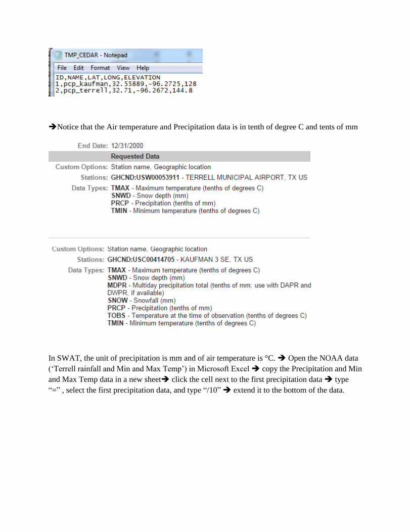
Notice that the Air temperature and Precipitation data is in tenth of degree C and tents of mm

In SWAT, the unit of precipitation is mm and of air temperature is °C. Open the NOAA data

(‘Terrell rainfall and Min and Max Temp’) in Microsoft Excel copy the Precipitation and Min

and Max Temp data in a new sheet click the cell next to the first precipitation data type

“=” , select the first precipitation data, and type “/10” extend it to the bottom of the data.

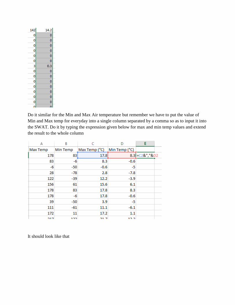
Do it similar for the Min and Max Air temperature but remember we have to put the value of

Min and Max temp for everyday into a single column separated by a comma so as to input it into

the SWAT. Do it by typing the expression given below for max and min temp values and extend

the result to the whole column

It should look like that

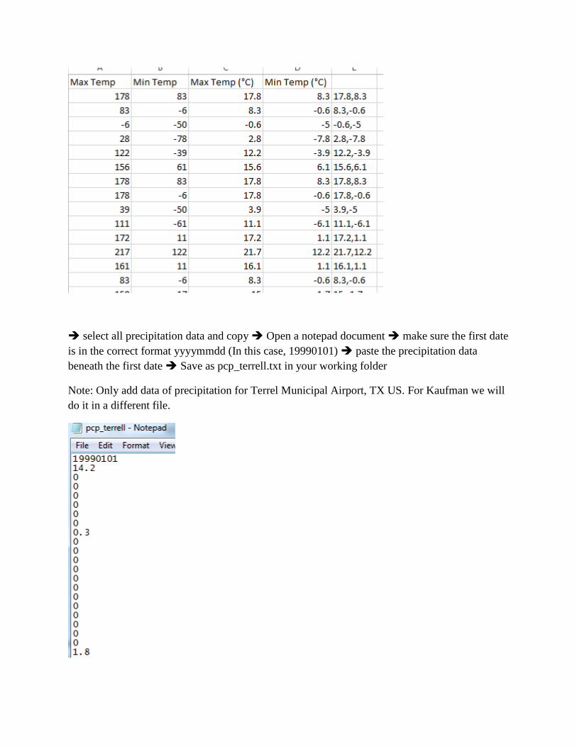
select all precipitation data and copy Open a notepad document make sure the first date

is in the correct format yyyymmdd (In this case, 19990101) paste the precipitation data

beneath the first date Save as pcp_terrell.txt in your working folder

Note: Only add data of precipitation for Terrel Municipal Airport, TX US. For Kaufman we will

do it in a different file.

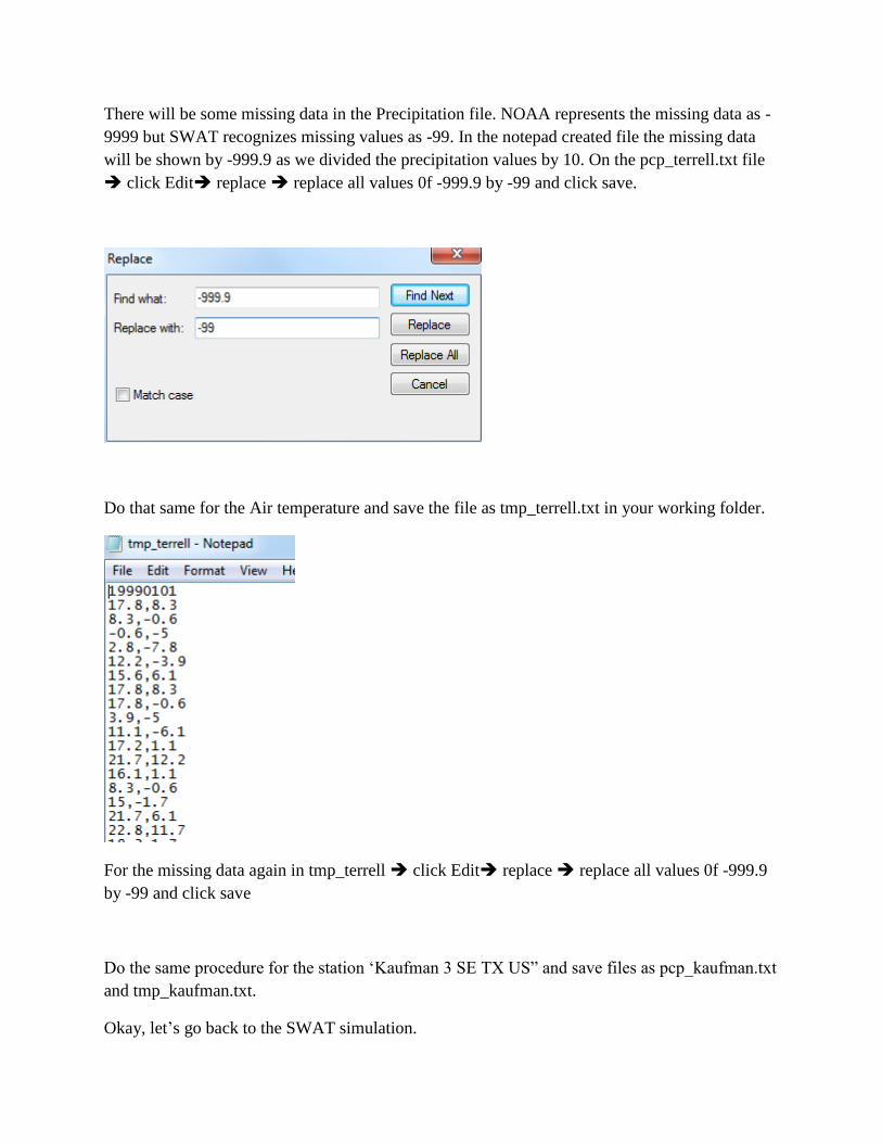
There will be some missing data in the Precipitation file. NOAA represents the missing data as -

9999 but SWAT recognizes missing values as -99. In the notepad created file the missing data

will be shown by -999.9 as we divided the precipitation values by 10. On the pcp_terrell.txt file

click Edit replace replace all values 0f -999.9 by -99 and click save.

Do that same for the Air temperature and save the file as tmp_terrell.txt in your working folder.

For the missing data again in tmp_terrell click Edit replace replace all values 0f -999.9

by -99 and click save

Do the same procedure for the station ‘Kaufman 3 SE TX US” and save files as pcp_kaufman.txt

and tmp_kaufman.txt.

Okay, let’s go back to the SWAT simulation.

1. Write Input Tables tab Weather Stations Weather Generator Data tab Select

WGEN_US_COOP_1970_2000 Ok Ok go to the Rainfall Data tab peg Raingages

go to the Precip Timestep box and in the drop-down menu select Daily go to the Locations

Table box and click on the open files folder icon Navigate to your working folder

highlight the file PCP_CEDAR.txt Add Ok go to the Temperature Data tab peg

Climate Stations click on the open files folder icon Navigate to your working folder

highlight TMP_CEDAR.txt add Ok Exit from the Weather Stations box.

Generate SWAT Input Files

1. Write Input Tables tab Write SWAT Input Tables Select All Create Tables Yes

Ok close window

Explanation: Many of the input data files required by the SWAT model are generated by

this step.

***If the .wgn file is not being written properly an error message will prevent you from

continuing this step. In order to fix this issue you must go to the folder where you are

saving your files. Double click “SWAT 2012” to open the Access software. Go to the

“wgnrng” and locate the ‘PR_W1’ and ‘PR_W2’ fields in the “CRNAME” column. Add

an underscore to the end of both of these fields (So it should be ‘PR_W1_’ and

‘PR_W2_’). Save the file, close Access and rerun the Write SWAT Input Tables.

Setup SWAT Simulation

1. SWAT Simulation tab Run SWAT Start Date: 1/1/1999 Ending Date: 12/31/2000

go to the Printout Settings box and peg Monthly Setup SWAT Run Ok Run

SWAT Ok Fini!!! close window

Explanation: The dates of the SWAT simulation and the printout frequency is specified

in this step. More SWAT input data files (CIO, COD, PCP.PCP and TMP.TMP) are

generated at this time. The Run SWAT command runs the SWAT executable.