Embed Size (px)
Citation preview
Bag-of-Words models
Lecture 9
Slides from: S. Lazebnik, A. Torralba, L. Fei-Fei, D. Lowe, C. Szurka
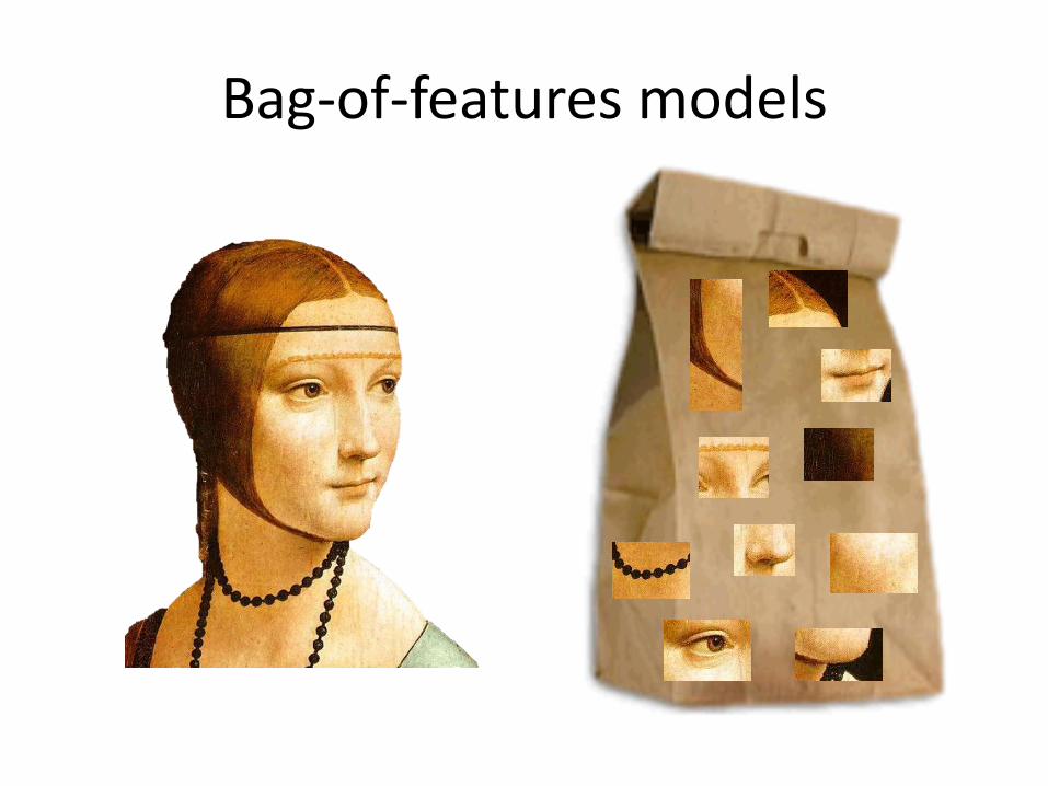
Bag-of-features models
Overview: Bag-of-features models
• Origins and motivation
• Image representation
• Discriminative methods– Nearest-neighbor classification
– Support vector machines
• Generative methods– Naïve Bayes
– Probabilistic Latent Semantic Analysis
• Extensions: incorporating spatial information
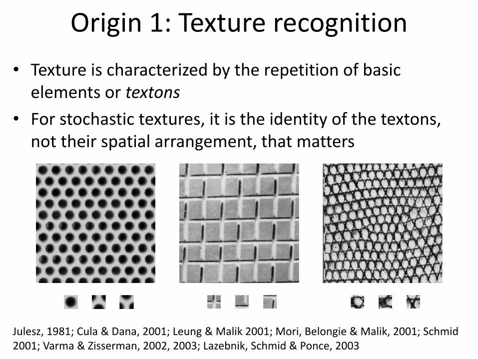
Origin 1: Texture recognition
• Texture is characterized by the repetition of basic elements or textons
• For stochastic textures, it is the identity of the textons, not their spatial arrangement, that matters
Julesz, 1981; Cula & Dana, 2001; Leung & Malik 2001; Mori, Belongie & Malik, 2001; Schmid2001; Varma & Zisserman, 2002, 2003; Lazebnik, Schmid & Ponce, 2003
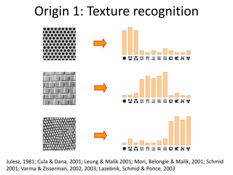
Origin 1: Texture recognition
Universal texton dictionary
histogram
Julesz, 1981; Cula & Dana, 2001; Leung & Malik 2001; Mori, Belongie & Malik, 2001; Schmid2001; Varma & Zisserman, 2002, 2003; Lazebnik, Schmid & Ponce, 2003
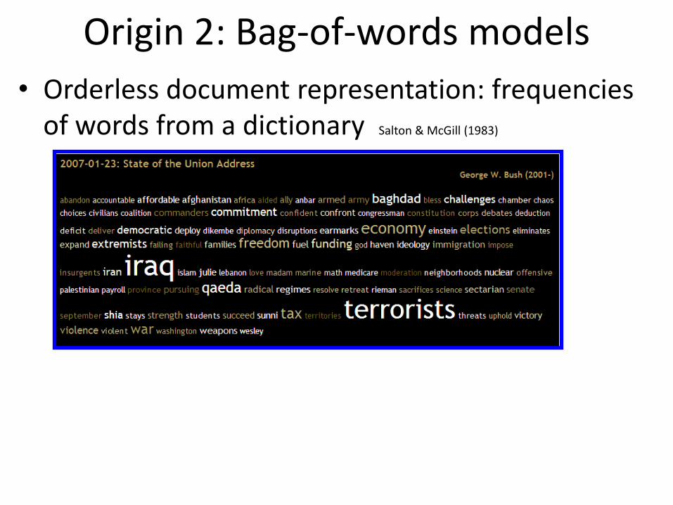
Origin 2: Bag-of-words models
• Orderless document representation: frequencies of words from a dictionary Salton & McGill (1983)
Origin 2: Bag-of-words models
US Presidential Speeches Tag Cloudhttp://chir.ag/phernalia/preztags/
• Orderless document representation: frequencies of words from a dictionary Salton & McGill (1983)
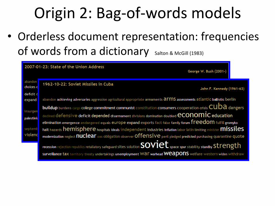
Origin 2: Bag-of-words models
US Presidential Speeches Tag Cloudhttp://chir.ag/phernalia/preztags/
• Orderless document representation: frequencies of words from a dictionary Salton & McGill (1983)
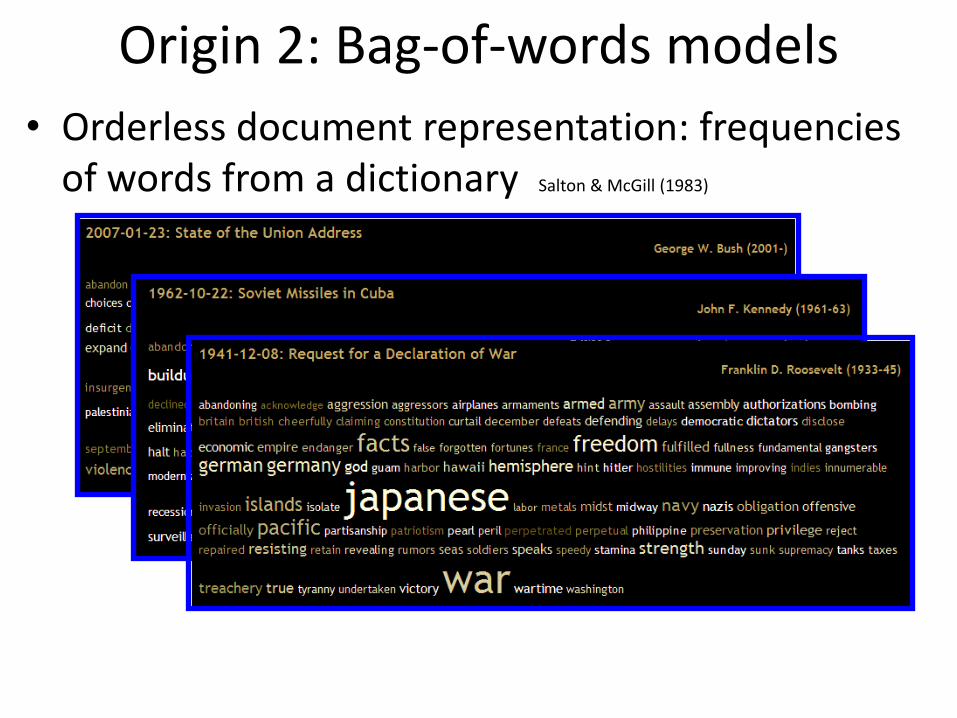
Origin 2: Bag-of-words models
US Presidential Speeches Tag Cloudhttp://chir.ag/phernalia/preztags/
• Orderless document representation: frequencies of words from a dictionary Salton & McGill (1983)
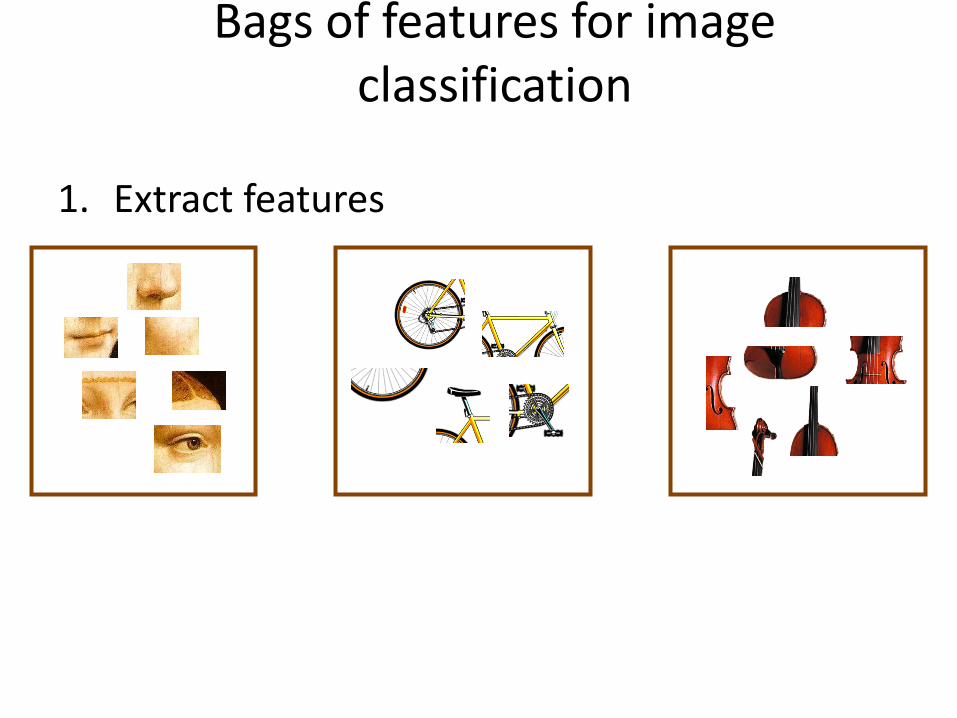
Bags of features for image classification
1. Extract features
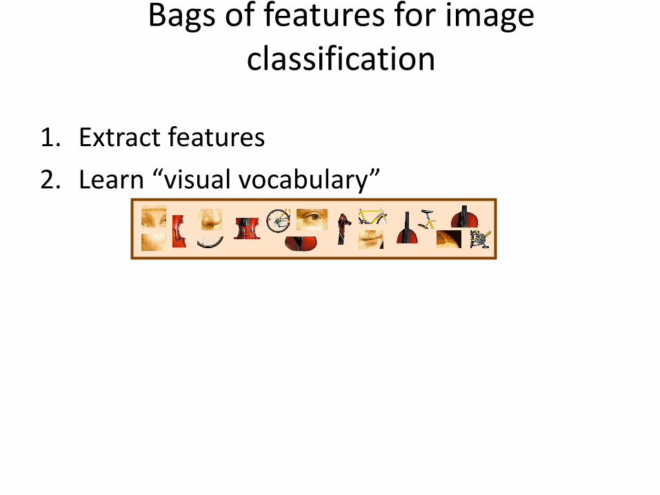
1. Extract features
2. Learn “visual vocabulary”
Bags of features for image classification
1. Extract features
2. Learn “visual vocabulary”
3. Quantize features using visual vocabulary
Bags of features for image classification
1. Extract features
2. Learn “visual vocabulary”
3. Quantize features using visual vocabulary
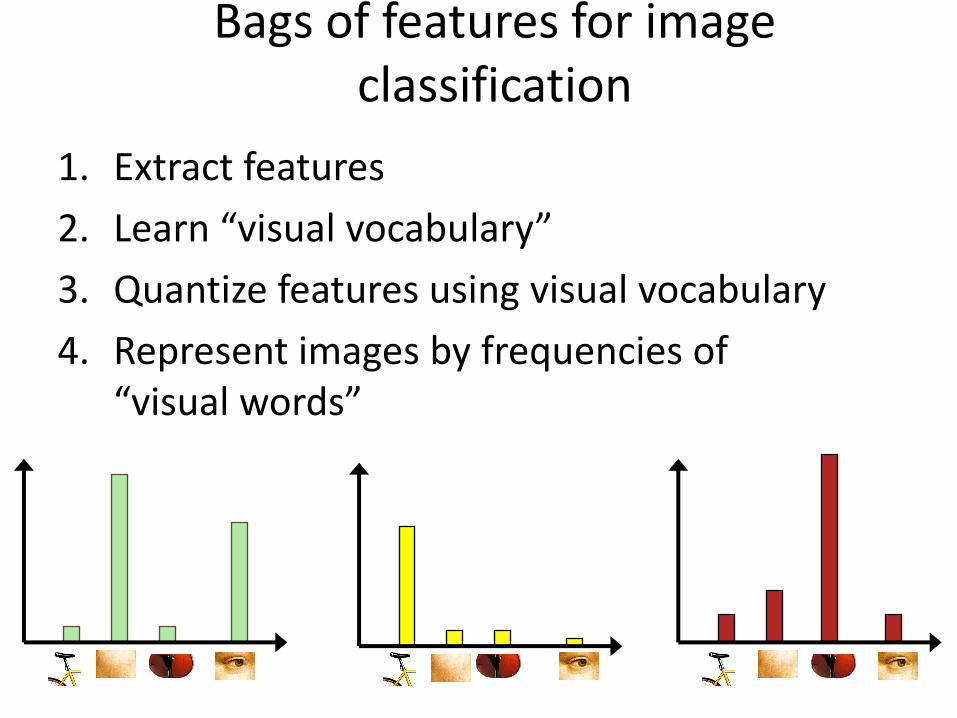
4. Represent images by frequencies of “visual words”
Bags of features for image classification
• Regular grid– Vogel & Schiele, 2003
– Fei-Fei & Perona, 2005
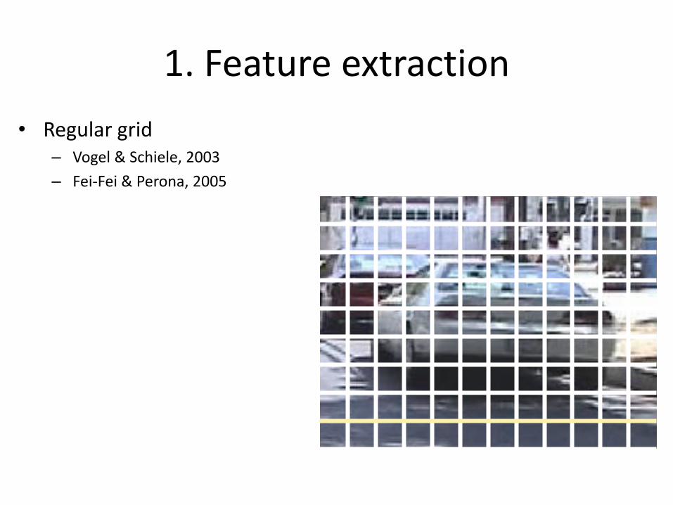
1. Feature extraction
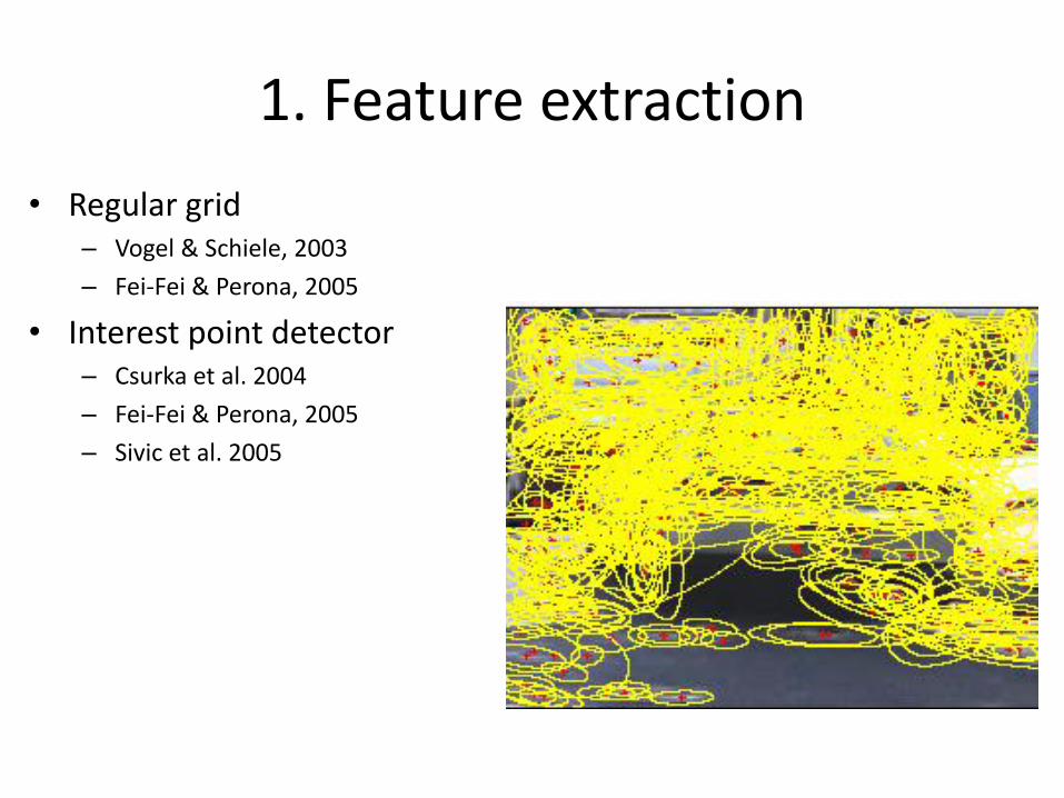
• Regular grid– Vogel & Schiele, 2003
– Fei-Fei & Perona, 2005
• Interest point detector– Csurka et al. 2004
– Fei-Fei & Perona, 2005
– Sivic et al. 2005
1. Feature extraction
• Regular grid– Vogel & Schiele, 2003
– Fei-Fei & Perona, 2005
• Interest point detector– Csurka et al. 2004
– Fei-Fei & Perona, 2005
– Sivic et al. 2005
• Other methods– Random sampling (Vidal-Naquet & Ullman, 2002)
– Segmentation-based patches (Barnard et al. 2003)
1. Feature extraction
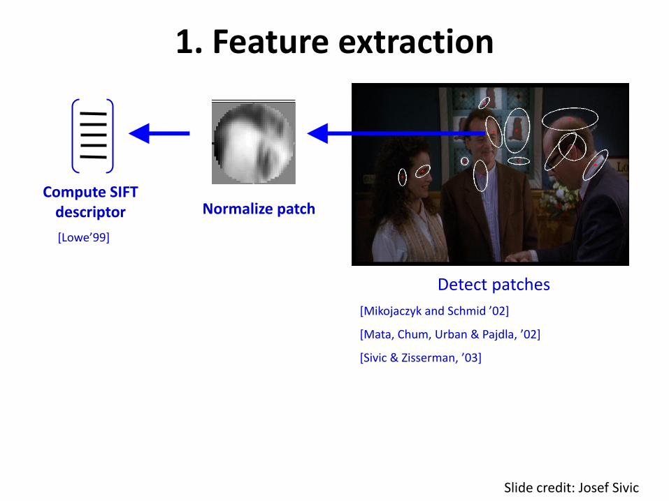
Normalize patch
Detect patches
[Mikojaczyk and Schmid ’02]
[Mata, Chum, Urban & Pajdla, ’02]
[Sivic & Zisserman, ’03]
Compute SIFT descriptor
[Lowe’99]
Slide credit: Josef Sivic
1. Feature extraction
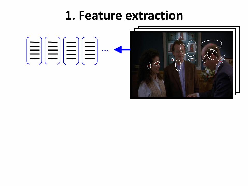
…
1. Feature extraction
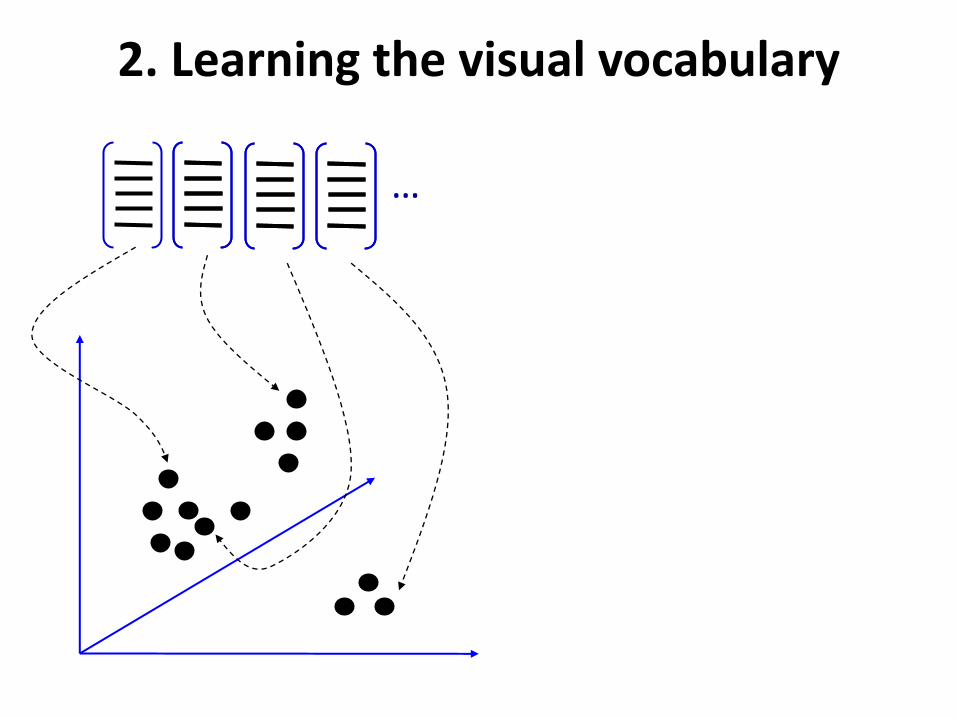
2. Learning the visual vocabulary
…
2. Learning the visual vocabulary
Clustering
…
Slide credit: Josef Sivic
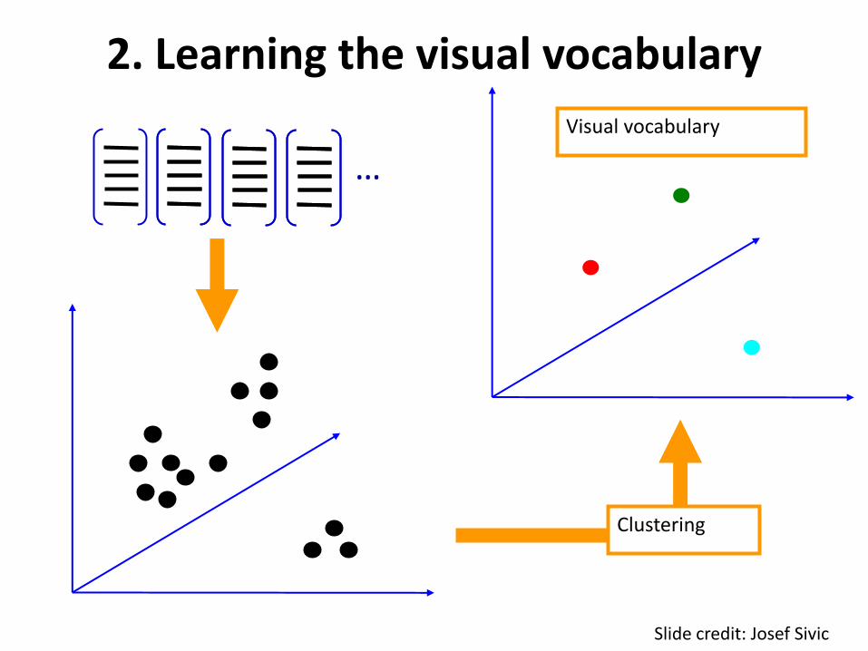
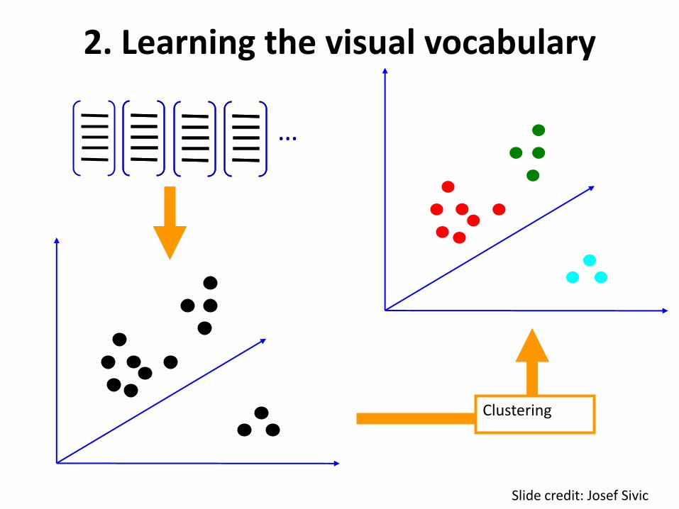
2. Learning the visual vocabulary
Clustering
…
Slide credit: Josef Sivic
Visual vocabulary
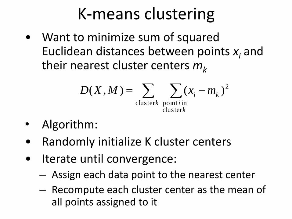
K-means clustering• Want to minimize sum of squared
Euclidean distances between points xi and their nearest cluster centers mk
• Algorithm:
• Randomly initialize K cluster centers
• Iterate until convergence:– Assign each data point to the nearest center
– Recompute each cluster center as the mean of all points assigned to it
kk
i
ki mxMXDcluster
clusterinpoint
2)(),(
From clustering to vector quantization• Clustering is a common method for learning a visual
vocabulary or codebook– Unsupervised learning process– Each cluster center produced by k-means becomes a
codevector– Codebook can be learned on separate training set– Provided the training set is sufficiently representative,
the codebook will be “universal”
• The codebook is used for quantizing features– A vector quantizer takes a feature vector and maps it to
the index of the nearest codevector in a codebook– Codebook = visual vocabulary– Codevector = visual word
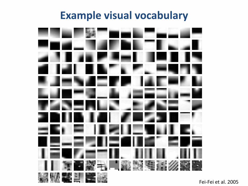
Example visual vocabulary
Fei-Fei et al. 2005
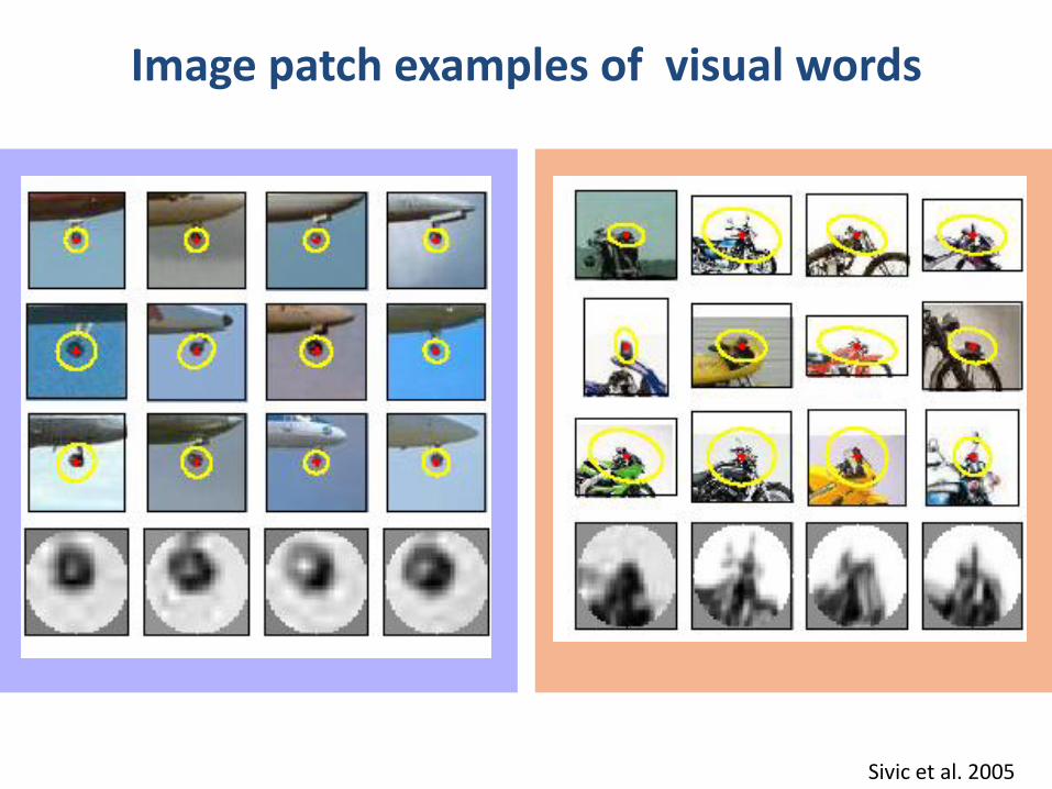
Image patch examples of visual words
Sivic et al. 2005
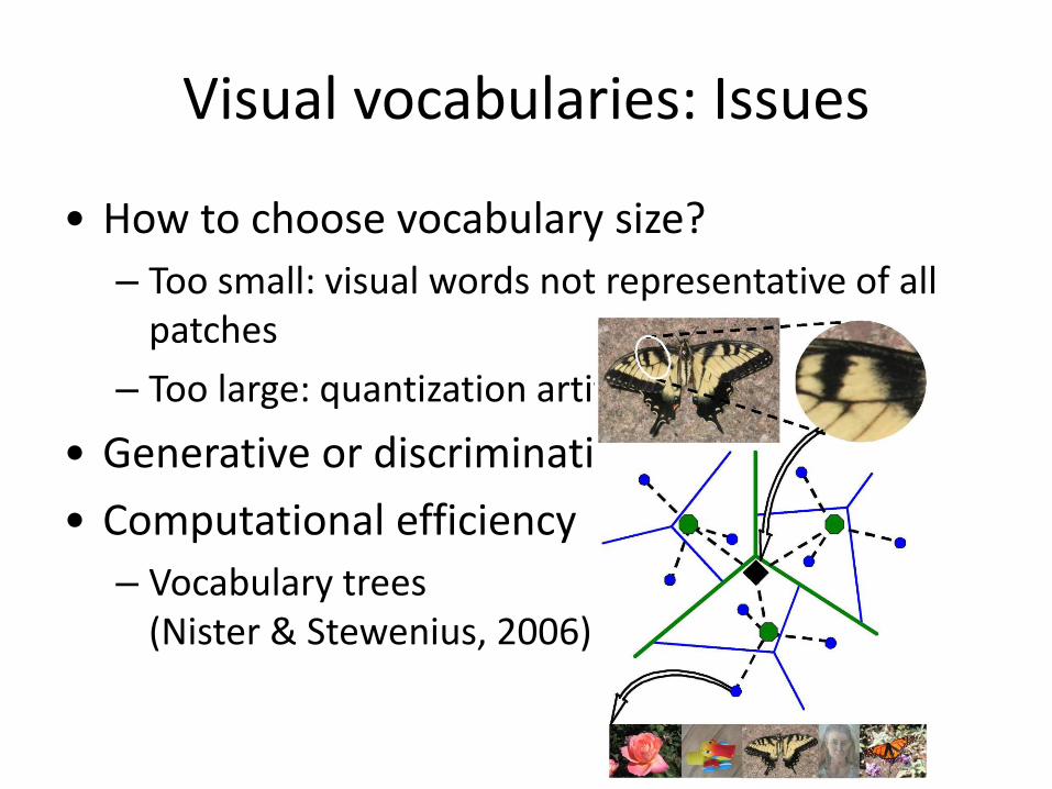
Visual vocabularies: Issues
• How to choose vocabulary size?
– Too small: visual words not representative of all patches
– Too large: quantization artifacts, overfitting
• Generative or discriminative learning?
• Computational efficiency
– Vocabulary trees (Nister & Stewenius, 2006)
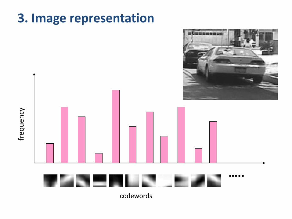
3. Image representation
…..
freq
uen
cy
codewords
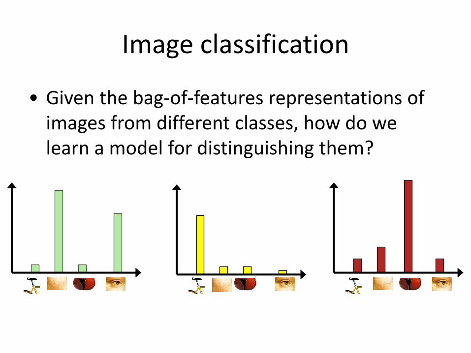
Image classification
• Given the bag-of-features representations of images from different classes, how do we learn a model for distinguishing them?
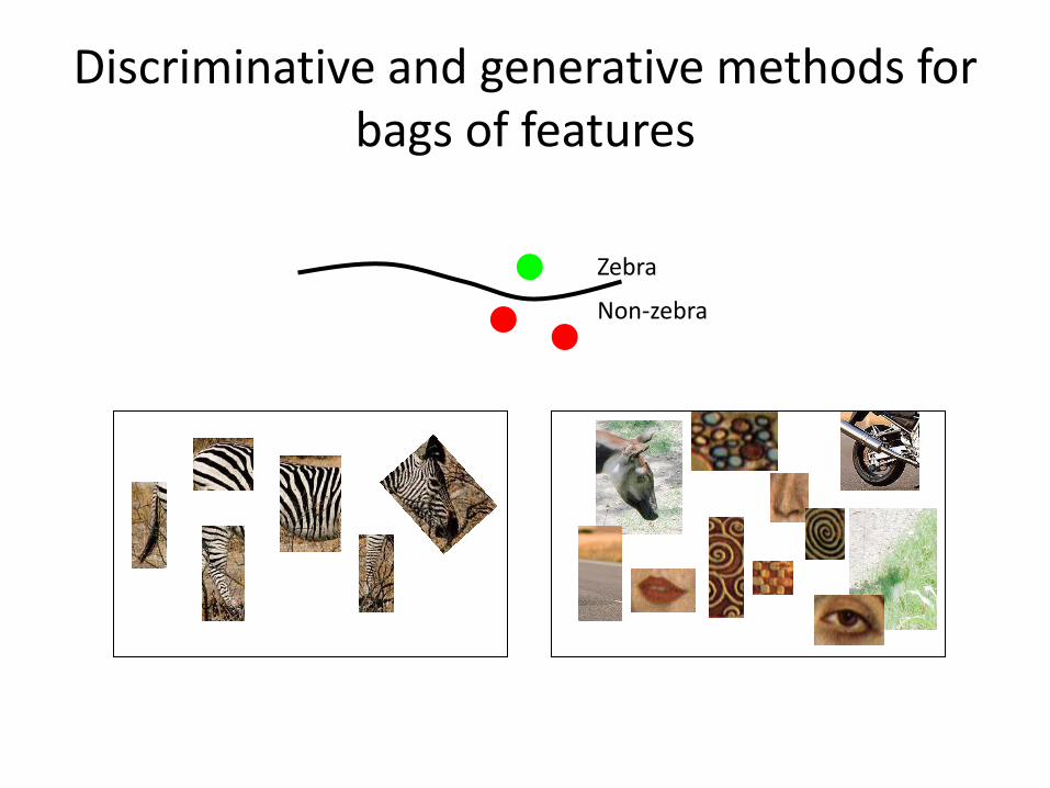
Discriminative and generative methods for bags of features
Zebra
Non-zebra

Image classification
• Given the bag-of-features representations of images from different classes, how do we learn a model for distinguishing them?
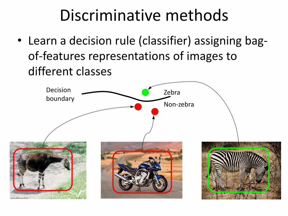
Discriminative methods
• Learn a decision rule (classifier) assigning bag-of-features representations of images to different classes
Zebra
Non-zebra
Decisionboundary
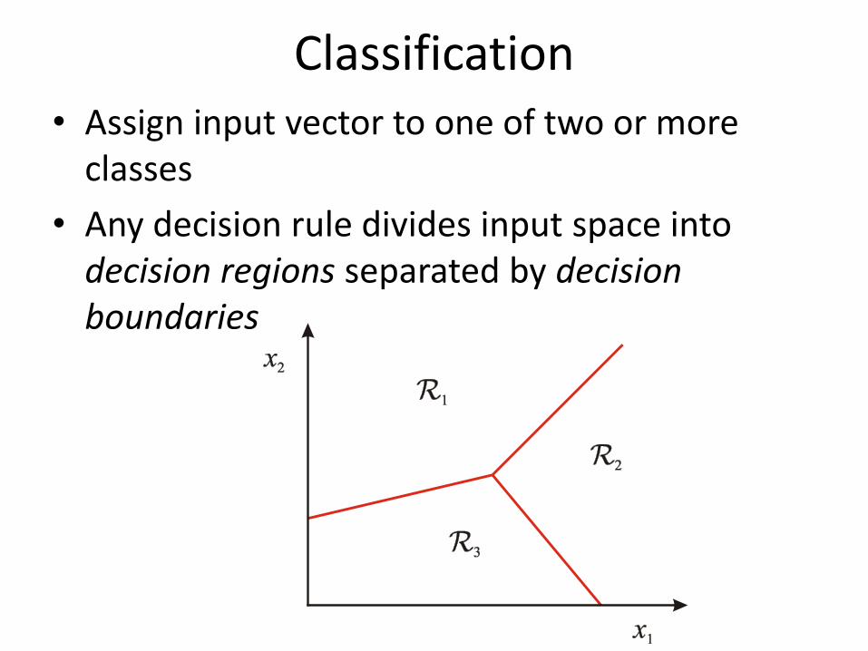
Classification• Assign input vector to one of two or more
classes
• Any decision rule divides input space into decision regions separated by decision boundaries
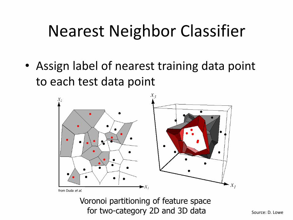
Nearest Neighbor Classifier
• Assign label of nearest training data point to each test data point
Voronoi partitioning of feature space for two-category 2D and 3D data
from Duda et al.
Source: D. Lowe
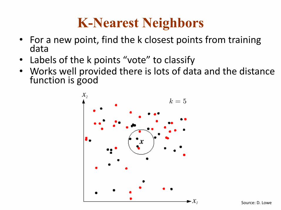
• For a new point, find the k closest points from training data
• Labels of the k points “vote” to classify• Works well provided there is lots of data and the distance
function is good
K-Nearest Neighbors
k = 5
Source: D. Lowe
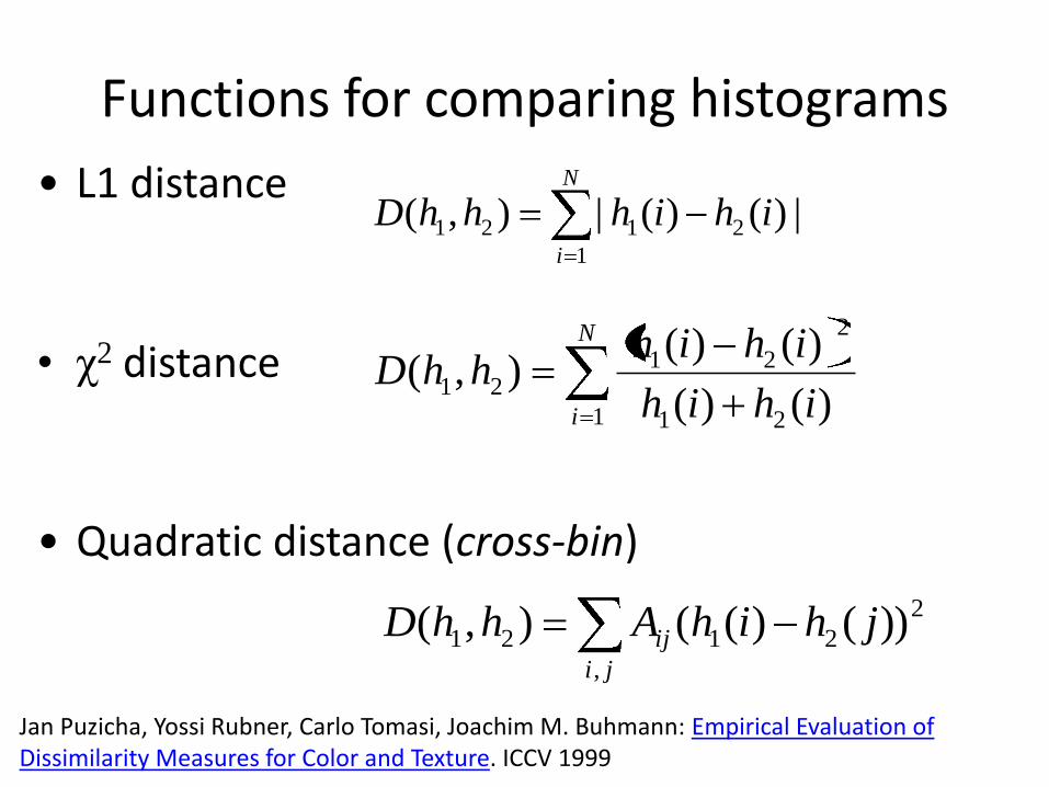
Functions for comparing histograms
• L1 distance
• χ2 distance
• Quadratic distance (cross-bin)
N
i
ihihhhD1
2121 |)()(|),(
Jan Puzicha, Yossi Rubner, Carlo Tomasi, Joachim M. Buhmann: Empirical Evaluation of Dissimilarity Measures for Color and Texture. ICCV 1999
N
i ihih
ihihhhD
1 21
2
2121
)()(
)()(),(
ji
ij jhihAhhD,
2
2121 ))()((),(
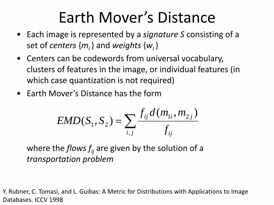
Earth Mover’s Distance• Each image is represented by a signature S consisting of a
set of centers {mi } and weights {wi }
• Centers can be codewords from universal vocabulary, clusters of features in the image, or individual features (in which case quantization is not required)
• Earth Mover’s Distance has the form
where the flows fij are given by the solution of a transportation problem
Y. Rubner, C. Tomasi, and L. Guibas: A Metric for Distributions with Applications to Image Databases. ICCV 1998
ji ij
jiij
f
mmdfSSEMD
,
21
21
),(),(
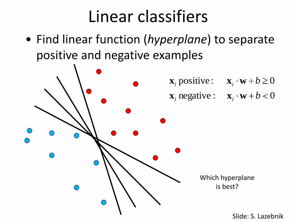
Linear classifiers• Find linear function (hyperplane) to separate
positive and negative examples
0:negative
0:positive
b
b
ii
ii
wxx
wxx
Which hyperplaneis best?
Slide: S. Lazebnik
Support vector machines
• Find hyperplane that maximizes the margin between the positive and negative examples
C. Burges, A Tutorial on Support Vector Machines for Pattern Recognition, Data Mining and Knowledge Discovery, 1998
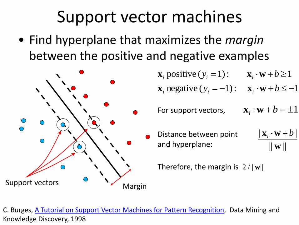
Support vector machines• Find hyperplane that maximizes the margin
between the positive and negative examples
1:1)(negative
1:1)( positive
by
by
iii
iii
wxx
wxx
MarginSupport vectors
C. Burges, A Tutorial on Support Vector Machines for Pattern Recognition, Data Mining and Knowledge Discovery, 1998
Distance between point and hyperplane: ||||
||
w
wx bi
For support vectors, 1bi wx
Therefore, the margin is 2 / ||w||
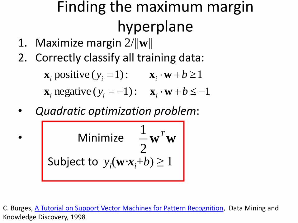
Finding the maximum margin hyperplane
1. Maximize margin 2/||w||
2. Correctly classify all training data:
• Quadratic optimization problem:
• Minimize
Subject to yi(w·xi+b) ≥ 1
C. Burges, A Tutorial on Support Vector Machines for Pattern Recognition, Data Mining and Knowledge Discovery, 1998
wwT
2
1
1:1)(negative
1:1)( positive
by
by
iii
iii
wxx
wxx
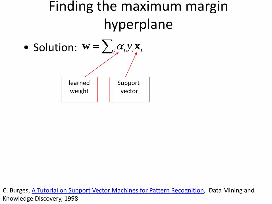
Finding the maximum margin hyperplane
• Solution: i iii y xw
C. Burges, A Tutorial on Support Vector Machines for Pattern Recognition, Data Mining and Knowledge Discovery, 1998
Support vector
learnedweight
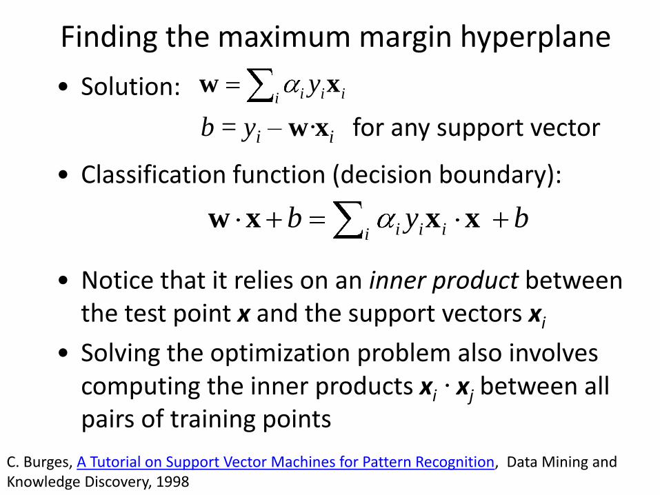
Finding the maximum margin hyperplane
• Solution:
b = yi – w·xi for any support vector
• Classification function (decision boundary):
• Notice that it relies on an inner product between the test point x and the support vectors xi
• Solving the optimization problem also involvescomputing the inner products xi · xj between all pairs of training points
i iii y xw
C. Burges, A Tutorial on Support Vector Machines for Pattern Recognition, Data Mining and Knowledge Discovery, 1998
bybi iii xxxw
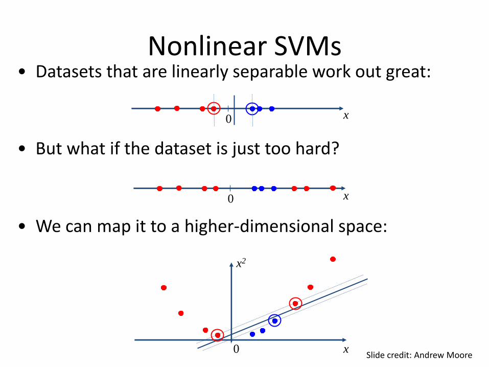
• Datasets that are linearly separable work out great:
• But what if the dataset is just too hard?
• We can map it to a higher-dimensional space:
0 x
0 x
0 x
x2
Nonlinear SVMs
Slide credit: Andrew Moore
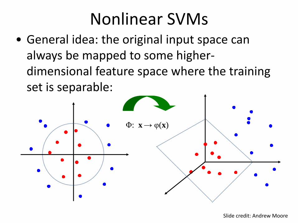
Φ: x → φ(x)
Nonlinear SVMs• General idea: the original input space can
always be mapped to some higher-dimensional feature space where the training set is separable:
Slide credit: Andrew Moore
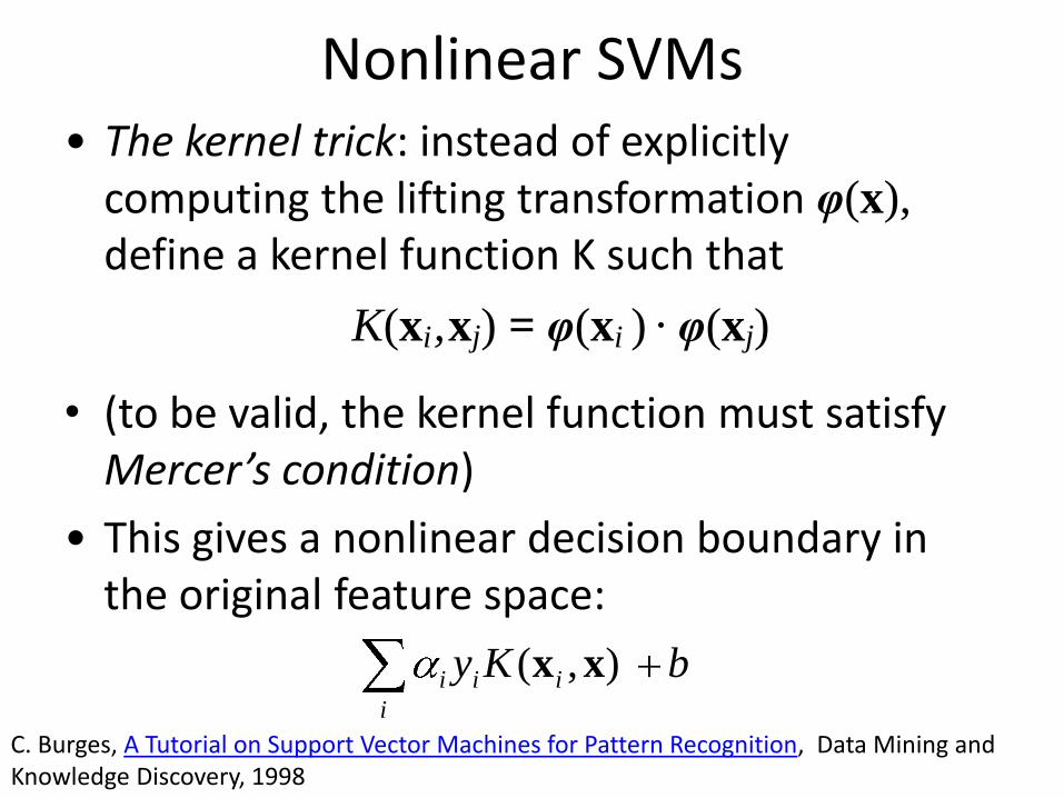
Nonlinear SVMs• The kernel trick: instead of explicitly
computing the lifting transformation φ(x),
define a kernel function K such that
K(xi,xj) = φ(xi ) · φ(xj)
• (to be valid, the kernel function must satisfy Mercer’s condition)
• This gives a nonlinear decision boundary in the original feature space:
bKyi
iii ),( xx
C. Burges, A Tutorial on Support Vector Machines for Pattern Recognition, Data Mining and Knowledge Discovery, 1998
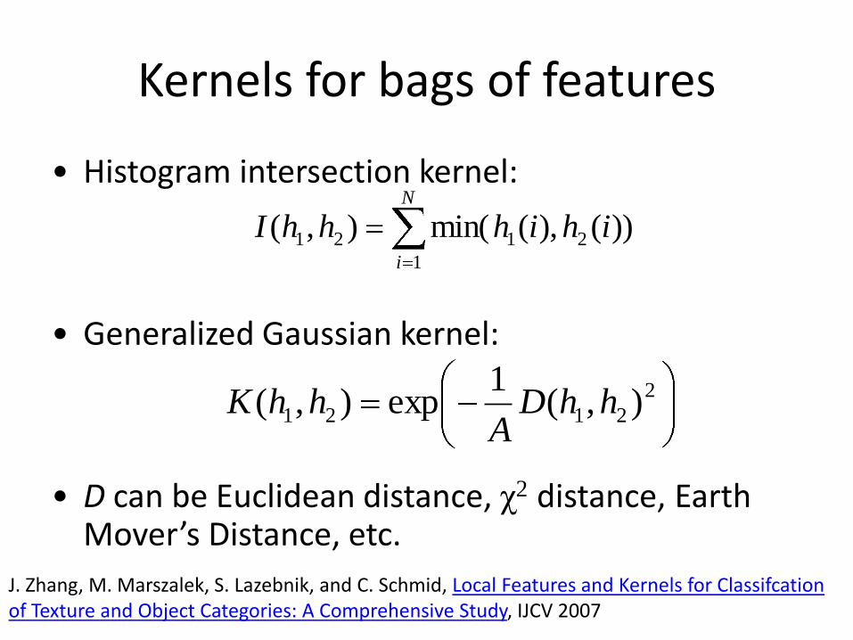
Kernels for bags of features
• Histogram intersection kernel:
• Generalized Gaussian kernel:
• D can be Euclidean distance, χ2 distance, Earth Mover’s Distance, etc.
N
i
ihihhhI1
2121 ))(),(min(),(
2
2121 ),(1
exp),( hhDA
hhK
J. Zhang, M. Marszalek, S. Lazebnik, and C. Schmid, Local Features and Kernels for Classifcation of Texture and Object Categories: A Comprehensive Study, IJCV 2007
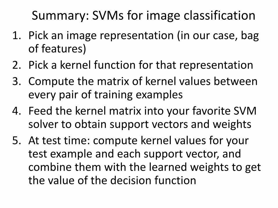
Summary: SVMs for image classification
1. Pick an image representation (in our case, bag of features)
2. Pick a kernel function for that representation
3. Compute the matrix of kernel values between every pair of training examples
4. Feed the kernel matrix into your favorite SVM solver to obtain support vectors and weights
5. At test time: compute kernel values for your test example and each support vector, and combine them with the learned weights to get the value of the decision function
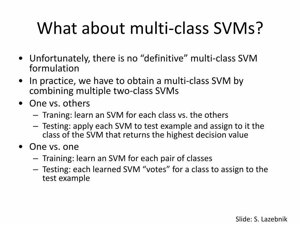
What about multi-class SVMs?
• Unfortunately, there is no “definitive” multi-class SVM formulation
• In practice, we have to obtain a multi-class SVM by combining multiple two-class SVMs
• One vs. others– Traning: learn an SVM for each class vs. the others– Testing: apply each SVM to test example and assign to it the
class of the SVM that returns the highest decision value
• One vs. one– Training: learn an SVM for each pair of classes– Testing: each learned SVM “votes” for a class to assign to the
test example
Slide: S. Lazebnik
SVMs: Pros and cons• Pros
– Many publicly available SVM packages:http://www.kernel-machines.org/software
– Kernel-based framework is very powerful, flexible– SVMs work very well in practice, even with very
small training sample sizes
• Cons– No “direct” multi-class SVM, must combine two-
class SVMs– Computation, memory
• During training time, must compute matrix of kernel values for every pair of examples
• Learning can take a very long time for large-scale problems
Slide: S. Lazebnik
Summary: Discriminative methods
• Nearest-neighbor and k-nearest-neighbor classifiers– L1 distance, χ2 distance, quadratic distance,
Earth Mover’s Distance
• Support vector machines– Linear classifiers– Margin maximization– The kernel trick– Kernel functions: histogram intersection, generalized
Gaussian, pyramid match– Multi-class
• Of course, there are many other classifiers out there– Neural networks, boosting, decision trees, …
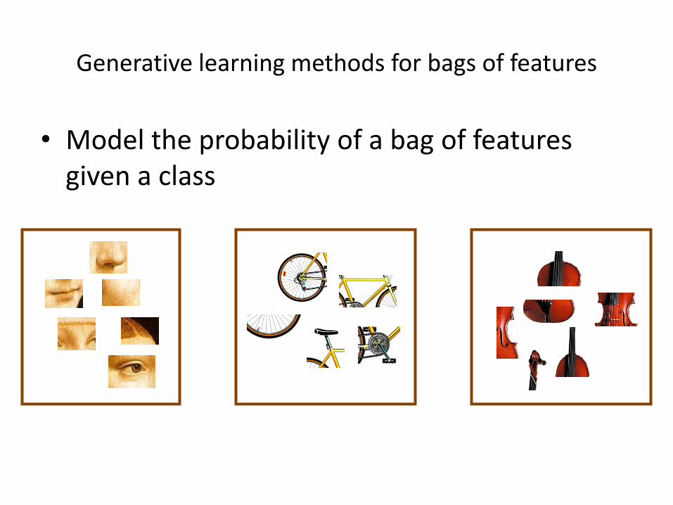
Generative learning methods for bags of features
• Model the probability of a bag of features given a class
Generative methods
• We will cover two models, both inspired by text document analysis:
– Naïve Bayes
– Probabilistic Latent Semantic Analysis
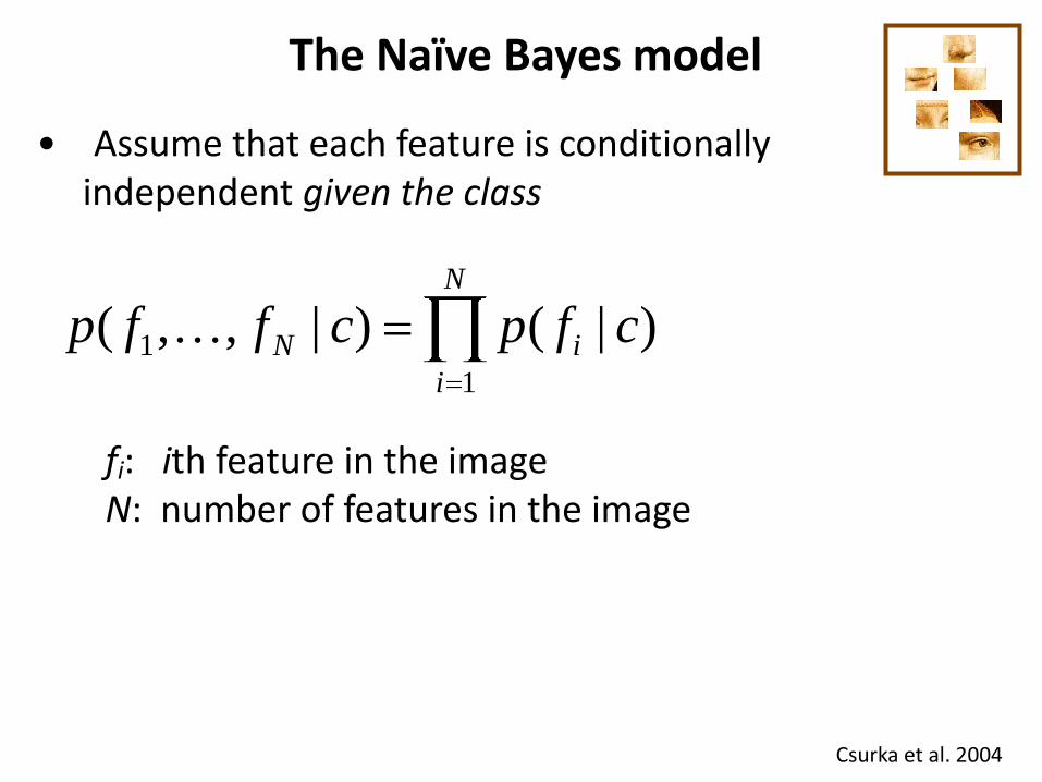
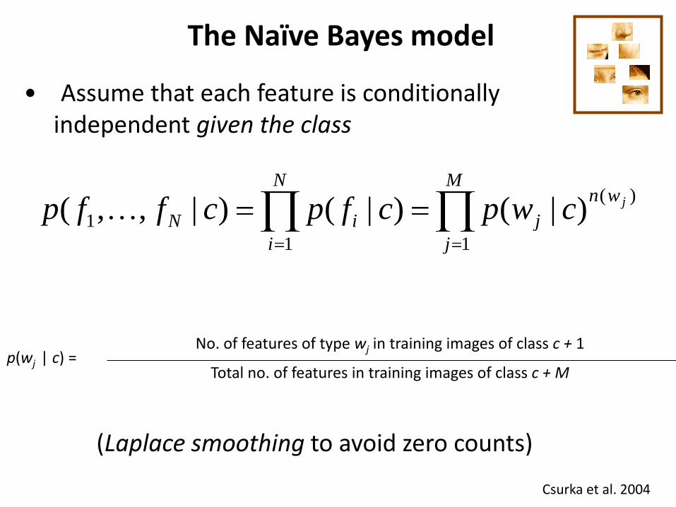
The Naïve Bayes model
Csurka et al. 2004
• Assume that each feature is conditionally independent given the class
fi: ith feature in the imageN: number of features in the image
N
i
iN cfpcffp1
1 )|()|,,(
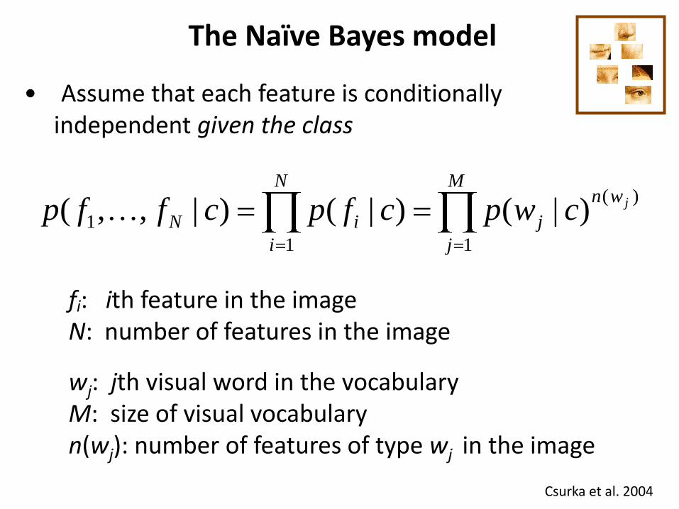
The Naïve Bayes model
Csurka et al. 2004
M
j
wn
j
N
i
iNjcwpcfpcffp
1
)(
1
1 )|()|()|,,(
• Assume that each feature is conditionally independent given the class
wj: jth visual word in the vocabularyM: size of visual vocabularyn(wj): number of features of type wj in the image
fi: ith feature in the imageN: number of features in the image
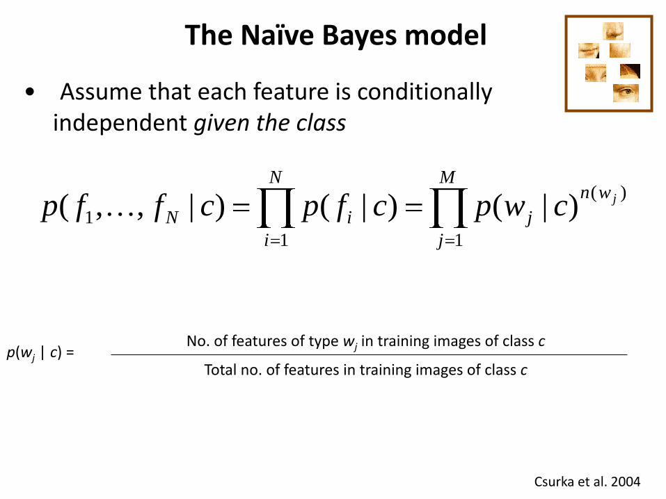
The Naïve Bayes model
Csurka et al. 2004
• Assume that each feature is conditionally independent given the class
No. of features of type wj in training images of class c
Total no. of features in training images of class cp(wj | c) =
M
j
wn
j
N
i
iNjcwpcfpcffp
1
)(
1
1 )|()|()|,,(
The Naïve Bayes model
Csurka et al. 2004
• Assume that each feature is conditionally independent given the class
No. of features of type wj in training images of class c + 1
Total no. of features in training images of class c + Mp(wj | c) =
(Laplace smoothing to avoid zero counts)
M
j
wn
j
N
i
iNjcwpcfpcffp
1
)(
1
1 )|()|()|,,(
M
j
jjc
M
j
wn
jc
cwpwncp
cwpcpc j
1
1
)(
)|(log)()(logmaxarg
)|()(maxarg*
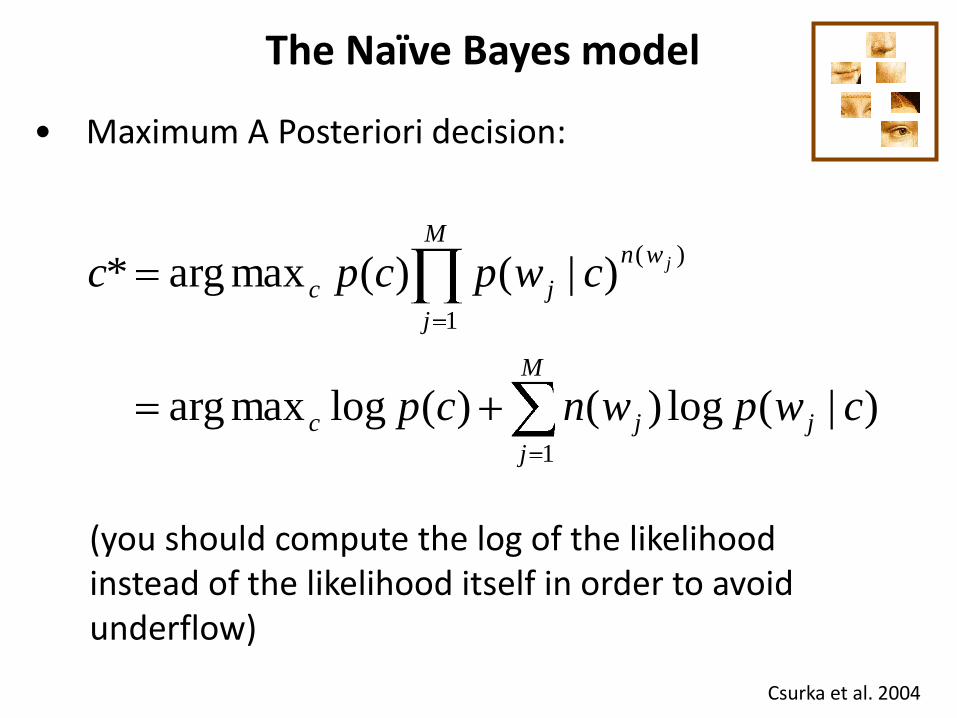
The Naïve Bayes model
Csurka et al. 2004
• Maximum A Posteriori decision:
(you should compute the log of the likelihood instead of the likelihood itself in order to avoid underflow)
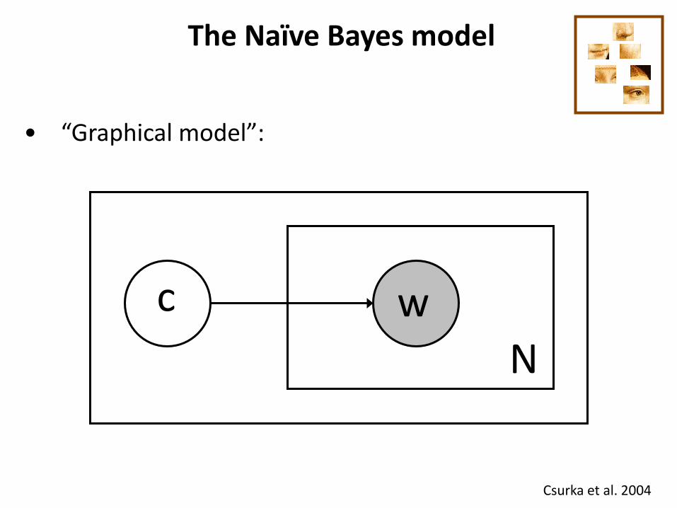
The Naïve Bayes model
Csurka et al. 2004
w
N
c
• “Graphical model”:
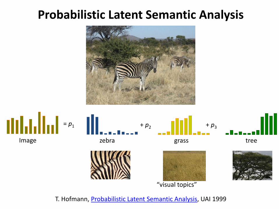
Probabilistic Latent Semantic Analysis
T. Hofmann, Probabilistic Latent Semantic Analysis, UAI 1999
zebra grass treeImage
= p1 + p2 + p3
“visual topics”
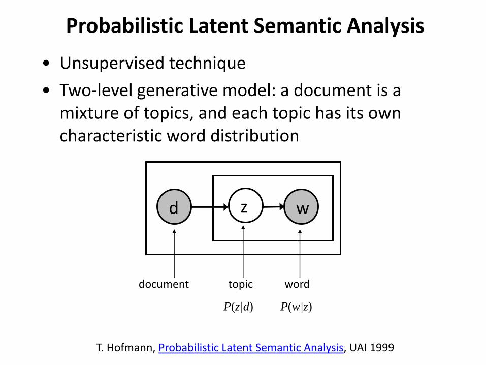
Probabilistic Latent Semantic Analysis
• Unsupervised technique
• Two-level generative model: a document is a mixture of topics, and each topic has its own characteristic word distribution
wd z
T. Hofmann, Probabilistic Latent Semantic Analysis, UAI 1999
document topic word
P(z|d) P(w|z)
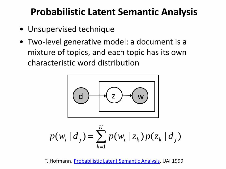
Probabilistic Latent Semantic Analysis
• Unsupervised technique
• Two-level generative model: a document is a mixture of topics, and each topic has its own characteristic word distribution
wd z
T. Hofmann, Probabilistic Latent Semantic Analysis, UAI 1999
K
k
jkkiji dzpzwpdwp1
)|()|()|(
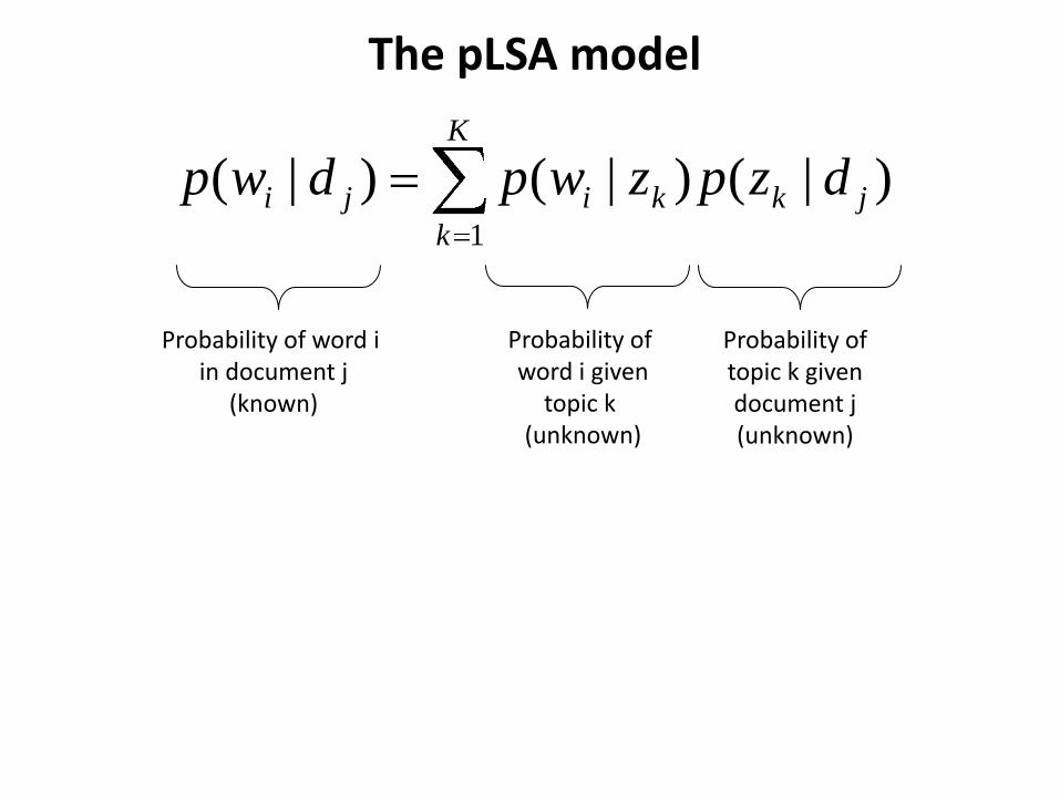
The pLSA model
K
k
jkkiji dzpzwpdwp1
)|()|()|(
Probability of word i in document j
(known)
Probability of word i given
topic k (unknown)
Probability oftopic k givendocument j(unknown)
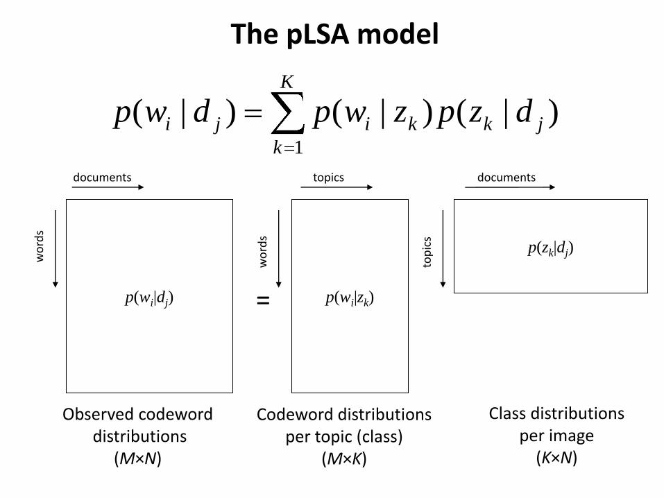
The pLSA model
Observed codeworddistributions
(M×N)
Codeword distributionsper topic (class)
(M×K)
Class distributionsper image
(K×N)
K
k
jkkiji dzpzwpdwp1
)|()|()|(
p(wi|dj) p(wi|zk)
p(zk|dj)
documents
wo
rds
wo
rds
topics
top
ics
documents
=
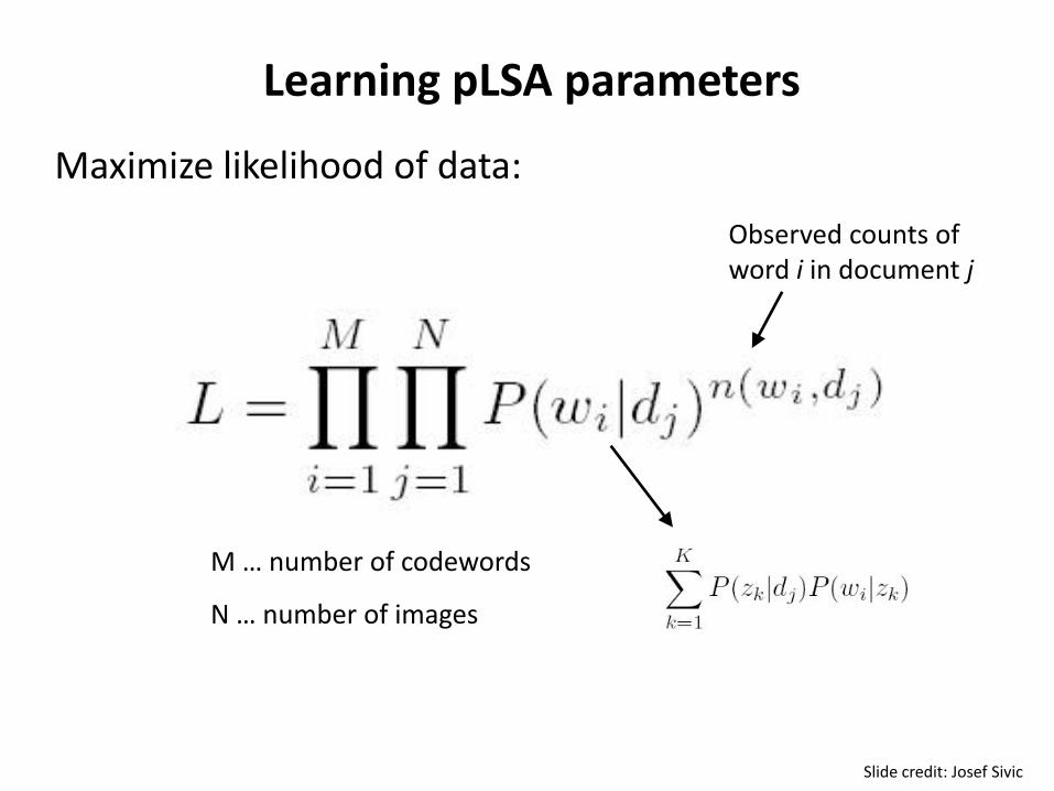
Maximize likelihood of data:
Observed counts of word i in document j
M … number of codewords
N … number of images
Slide credit: Josef Sivic
Learning pLSA parameters
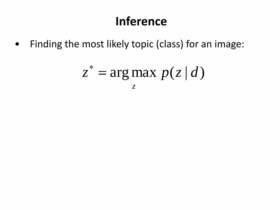
Inference
)|(maxarg dzpzz
• Finding the most likely topic (class) for an image:
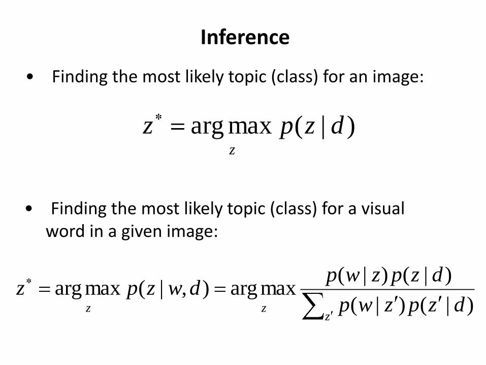
Inference
)|(maxarg dzpzz
• Finding the most likely topic (class) for an image:
zzz dzpzwp
dzpzwpdwzpz
)|()|(
)|()|(maxarg),|(maxarg
• Finding the most likely topic (class) for a visualword in a given image:
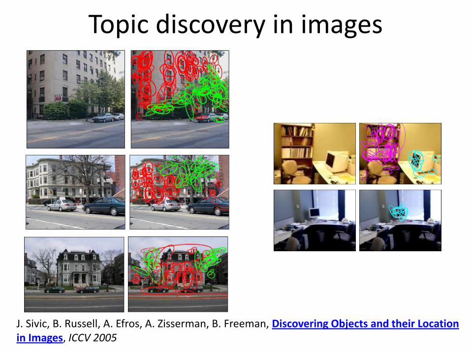
Topic discovery in images
J. Sivic, B. Russell, A. Efros, A. Zisserman, B. Freeman, Discovering Objects and their Location in Images, ICCV 2005
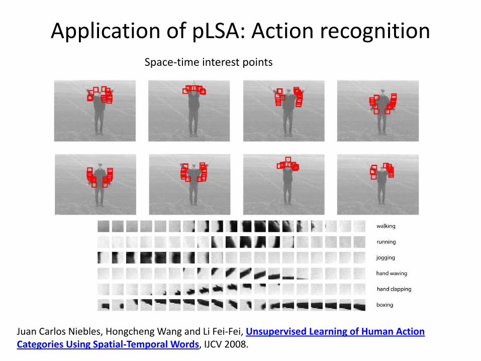
Application of pLSA: Action recognition
Juan Carlos Niebles, Hongcheng Wang and Li Fei-Fei, Unsupervised Learning of Human Action Categories Using Spatial-Temporal Words, IJCV 2008.
Space-time interest points
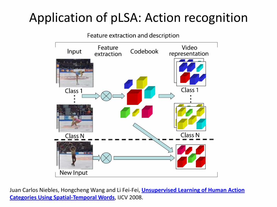
Application of pLSA: Action recognition
Juan Carlos Niebles, Hongcheng Wang and Li Fei-Fei, Unsupervised Learning of Human Action Categories Using Spatial-Temporal Words, IJCV 2008.
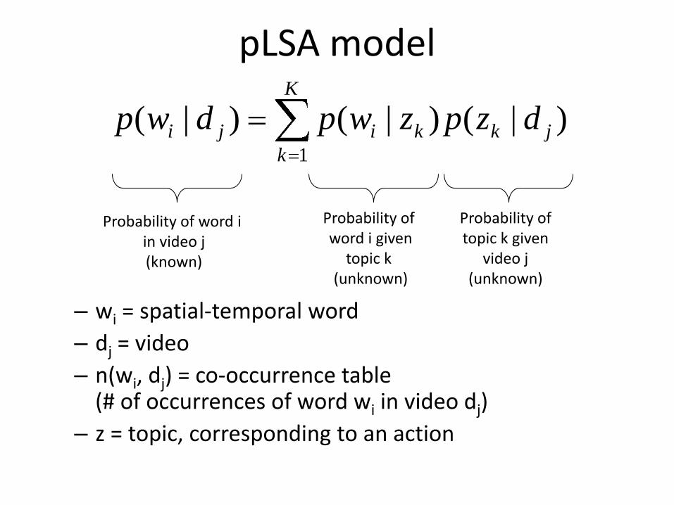
pLSA model
– wi = spatial-temporal word
– dj = video
– n(wi, dj) = co-occurrence table (# of occurrences of word wi in video dj)
– z = topic, corresponding to an action
K
k
jkkiji dzpzwpdwp1
)|()|()|(
Probability of word i in video j(known)
Probability of word i given
topic k (unknown)
Probability oftopic k given
video j(unknown)
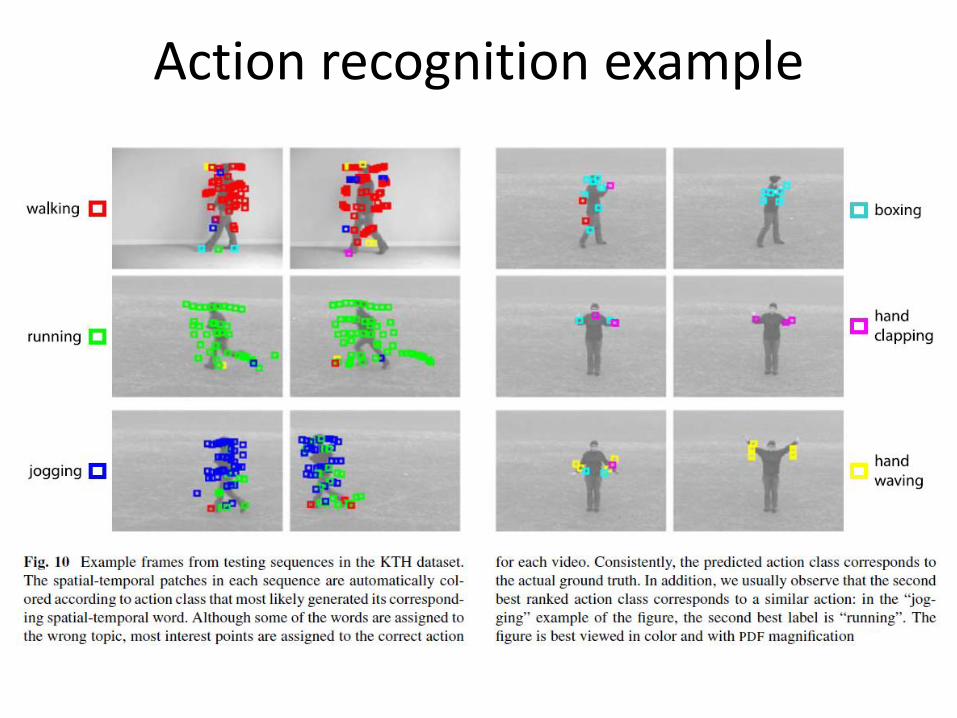
Action recognition example
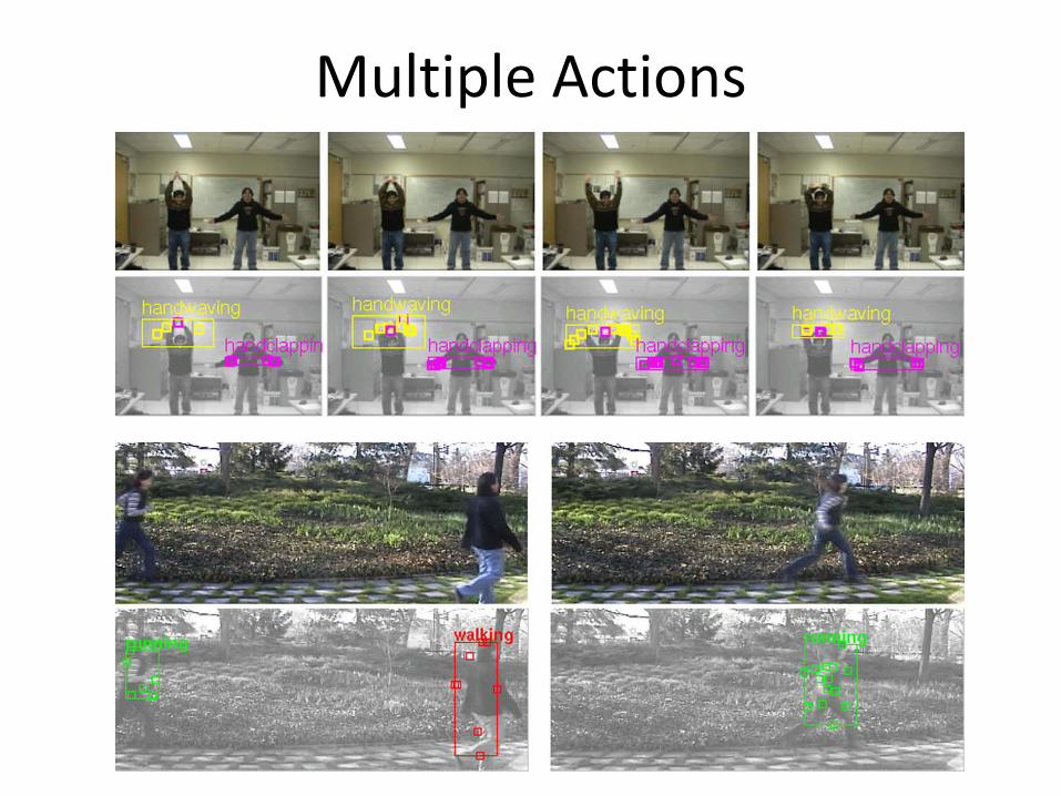
Multiple Actions
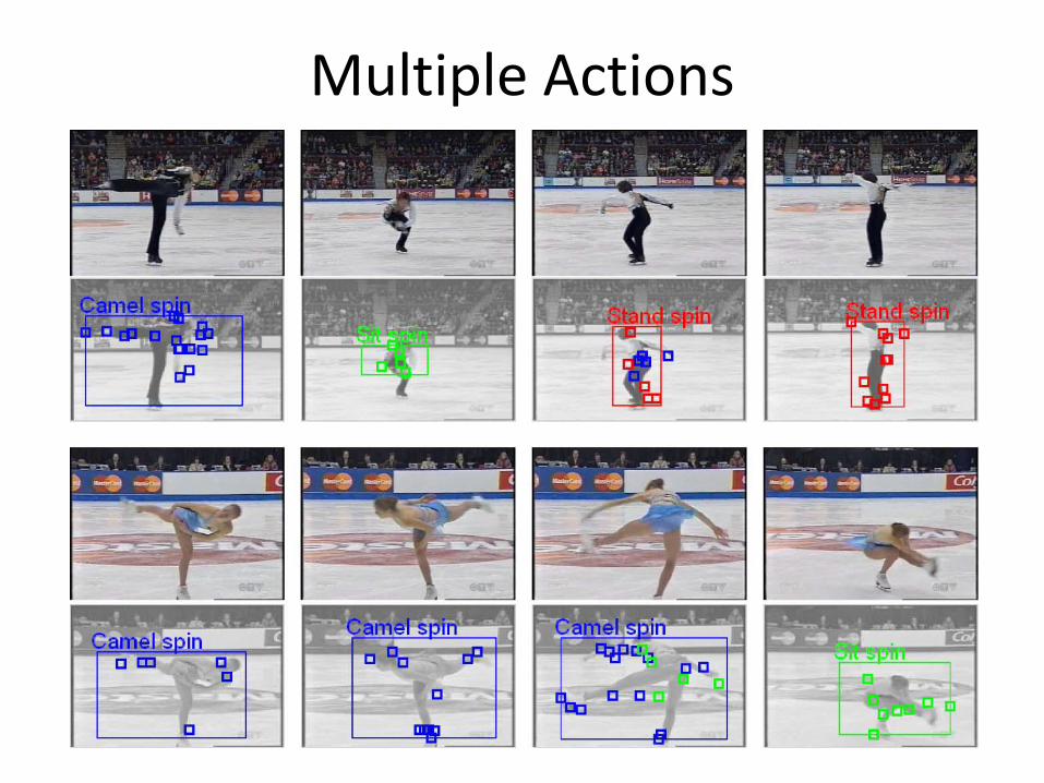
Multiple Actions
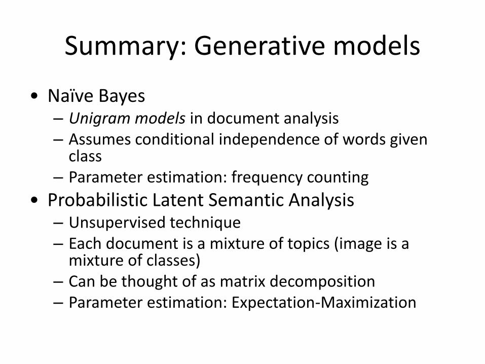
Summary: Generative models
• Naïve Bayes– Unigram models in document analysis– Assumes conditional independence of words given
class– Parameter estimation: frequency counting
• Probabilistic Latent Semantic Analysis– Unsupervised technique– Each document is a mixture of topics (image is a
mixture of classes)– Can be thought of as matrix decomposition– Parameter estimation: Expectation-Maximization
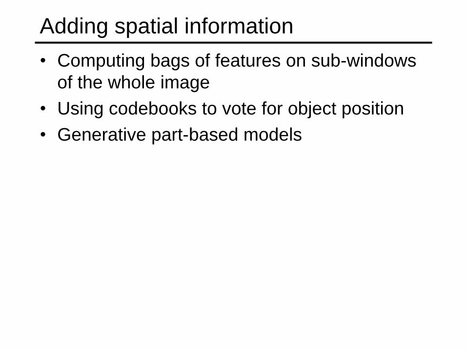
Adding spatial information
• Computing bags of features on sub-windows
of the whole image
• Using codebooks to vote for object position
• Generative part-based models
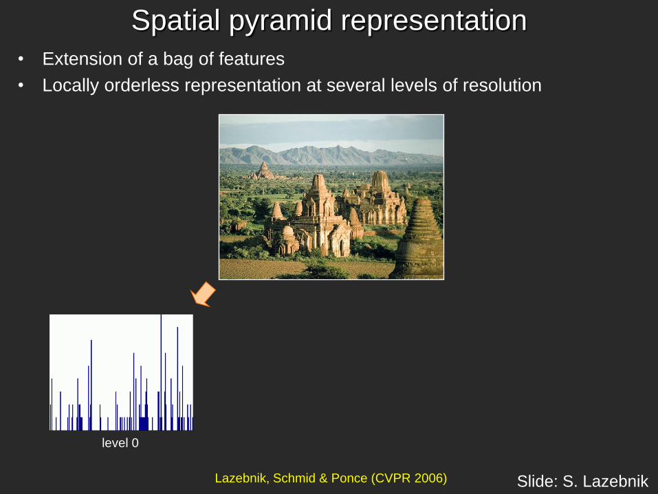
Spatial pyramid representation
• Extension of a bag of features
• Locally orderless representation at several levels of resolution
level 0
Lazebnik, Schmid & Ponce (CVPR 2006) Slide: S. Lazebnik
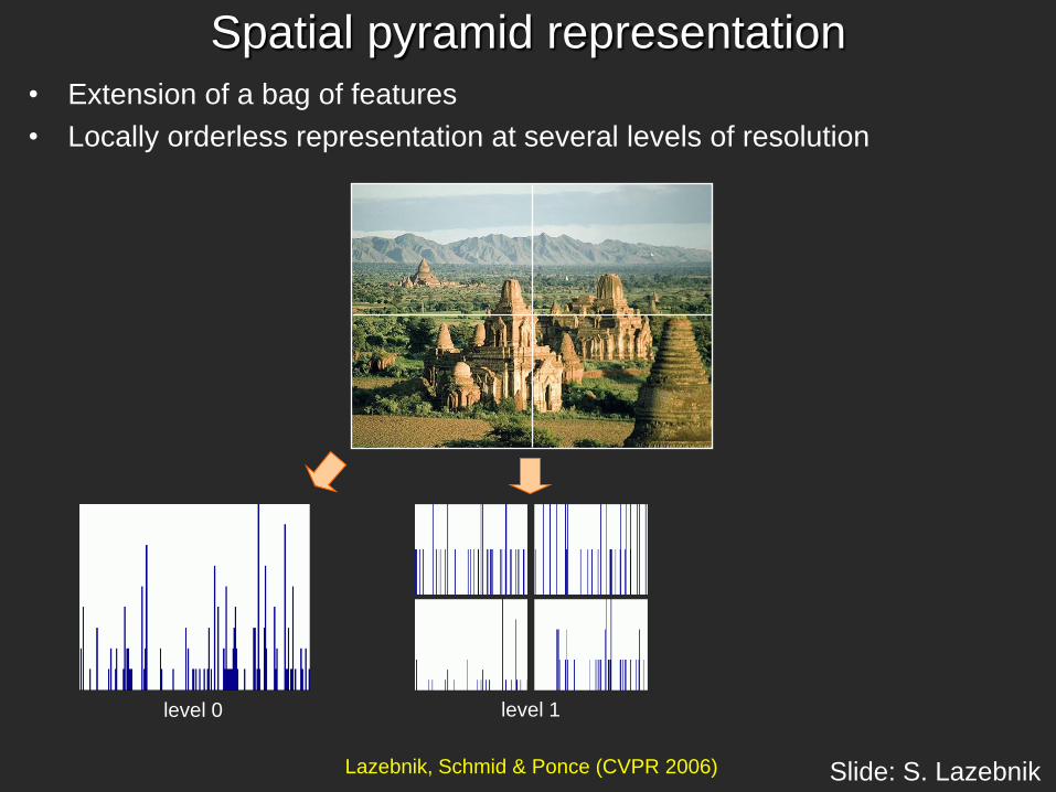
Spatial pyramid representation
• Extension of a bag of features
• Locally orderless representation at several levels of resolution
level 0 level 1
Lazebnik, Schmid & Ponce (CVPR 2006) Slide: S. Lazebnik
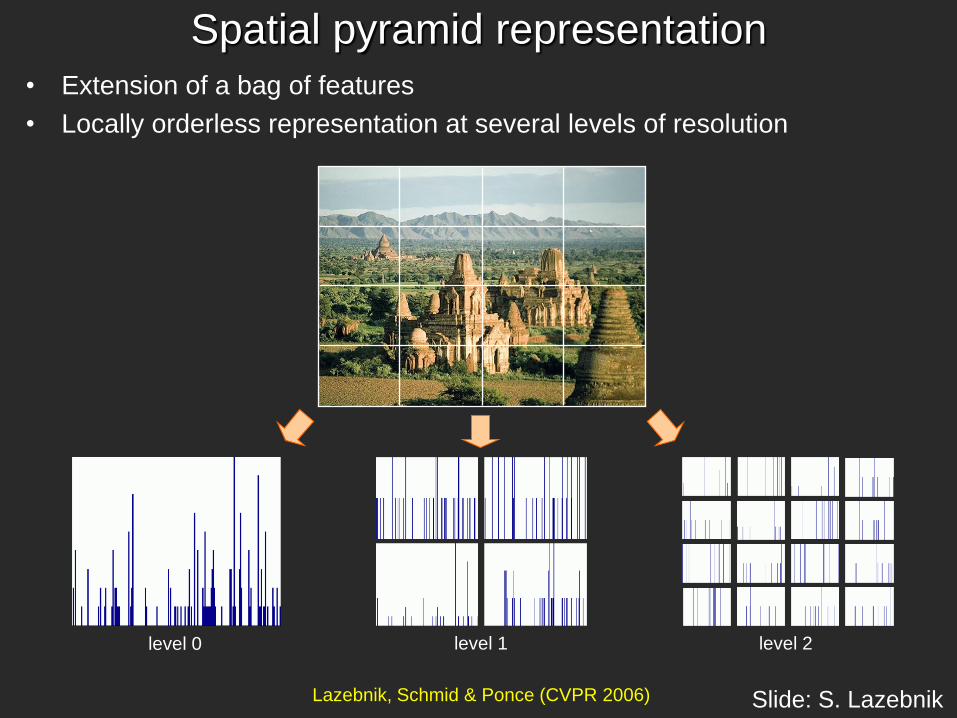
Spatial pyramid representation
level 0 level 1 level 2
• Extension of a bag of features
• Locally orderless representation at several levels of resolution
Lazebnik, Schmid & Ponce (CVPR 2006) Slide: S. Lazebnik
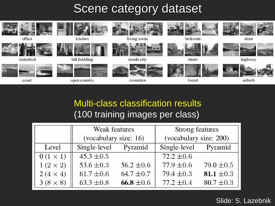
Scene category dataset
Multi-class classification results
(100 training images per class)
Slide: S. Lazebnik
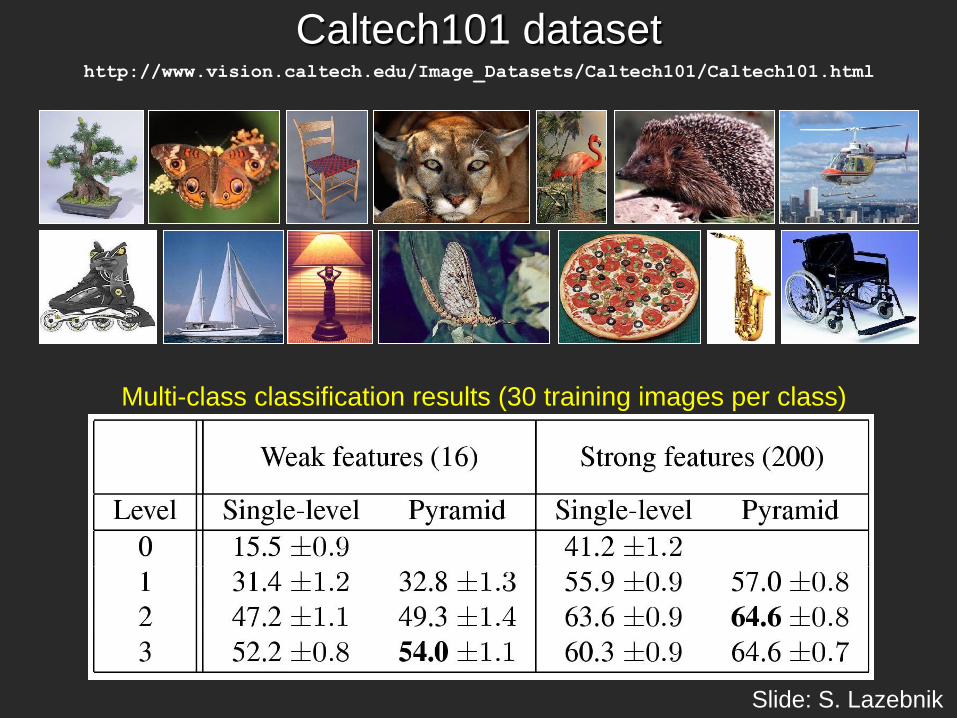
Caltech101 datasethttp://www.vision.caltech.edu/Image_Datasets/Caltech101/Caltech101.html
Multi-class classification results (30 training images per class)
Slide: S. Lazebnik
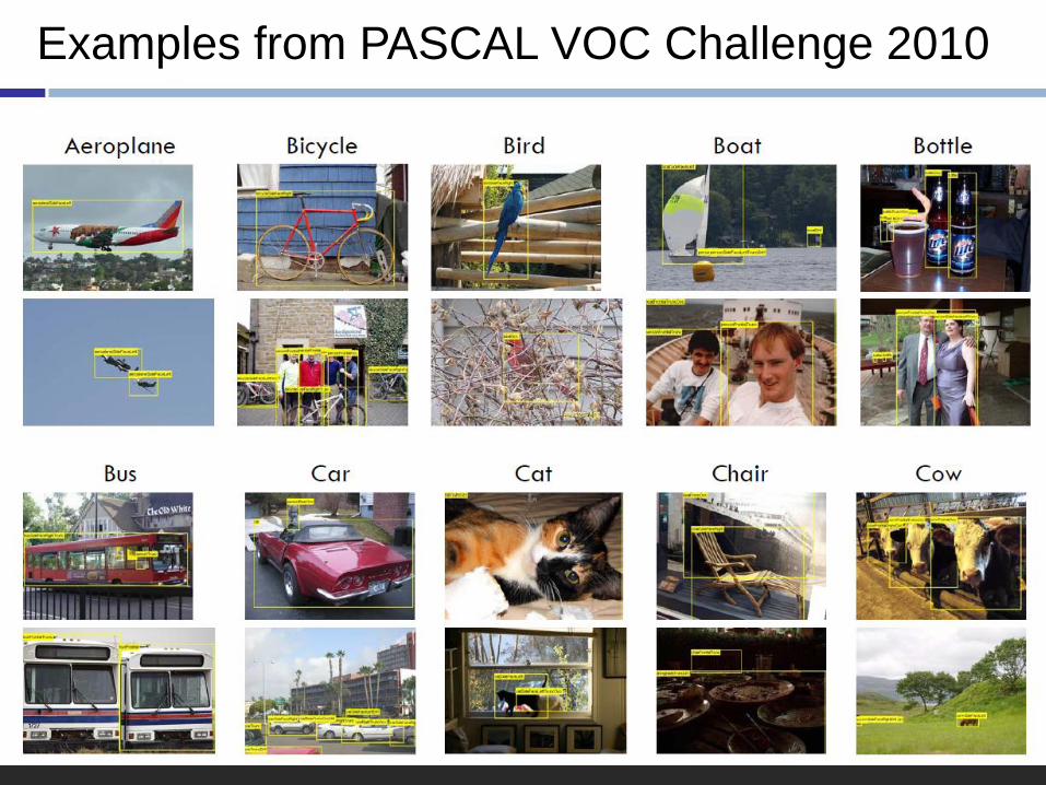
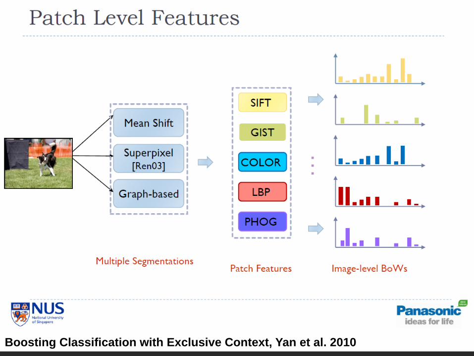
Examples from PASCAL VOC Challenge 2010
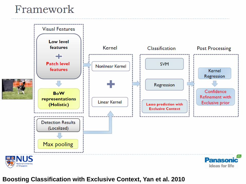
Boosting Classification with Exclusive Context, Yan et al. 2010
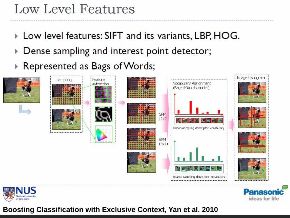
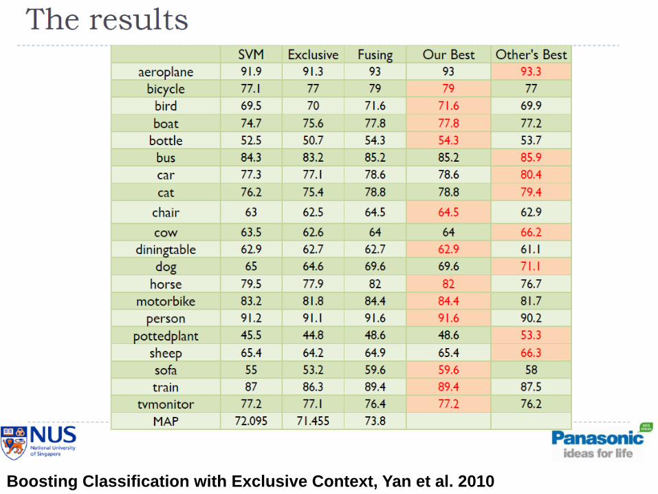
Boosting Classification with Exclusive Context, Yan et al. 2010
Boosting Classification with Exclusive Context, Yan et al. 2010
Boosting Classification with Exclusive Context, Yan et al. 2010