Balancing Admission Control, Speedup, and Waiting inService Systems

Carri W. ChanColumbia Business School, New York, NY cwchan@columbia.edu

Galit Yom-TovIsrael Institute of Technology, Haifa, Israel galit@technion.edu

November 11, 2014

In a number of service settings, customer waiting, admission control, and speedup of service rates can occur during

periods of congestion. For example, in a healthcare setting, this means that patients who require care may be sent to

other, less ideal service outlets or hospital units. As expected, this comes at a cost to patient outcomes. In this work, we

examine a multi-server queueing system which allows for admission control and speedup. We use dynamic programming

to characterize properties of the optimal control and find that in some instances, the optimal policy has a simple form of a

threshold policy. Leveraging this insight, we examine a queueing system where speedup is used when the number in the

system exceeds some threshold and admission control is usedwhen the number in the system exceeds some (potentially

different) threshold. Using fluid analysis and a loss model,we establish approximations for the probability of speedup, the

probability of admission control, and the expected queue length. We use the approximation analysis to characterize the

region of the optimal solution and develop a greedy heuristic to derive a near optimal solution to the original optimization

problem. We use simulation to demonstrate the quality of these approximations and find they can be quite accurate and

robust. This analysis can provide insight to system administrators as they evaluate how to balance admission and speedup

control—deciding when and to what extent to use each.

Key words: Queueing models, admission control, service rate control, dynamic programming, state-dependent queues,

healthcare operations

1. Introduction

Providing high quality service is of paramount importance for many service systems. Unfortunately, when

a system becomes congested, this is not always possible. A number of approaches have been considered

and adopted to navigate these periods of congestion. For instance, admission control whereby customers

are denied service (presumably finding service elsewhere orreturning later) has arisen in hospital set-

tings (Kim et al. 2014), call-centers (Ormeci 2004), and general service systems (Ata and Shneorson 2006).

Alternatively, increasing service rate (with a sacrifice toquality) has also been considered in Intensive Care

Units (ICUs) (Kc and Terwiesch 2012), production lines (Powell and Schultz 2004), email contact centers

(Hasija et al. 2010), and general service systems (Ata and Shneorson 2006). In this work, we consider how

to balance admission and service rate control in a multi-server setting in order to provide high quality service

to as many customers as possible.

1

2

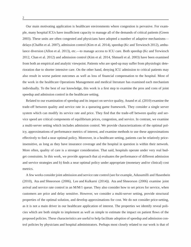
Our main motivating application is healthcare environments where congestion is pervasive. For exam-

ple, many hospital ICUs have insufficient capacity to manageall of the demands of critical patients (Green

2003). These units are often congested and physicians have adopted a number of adaptive mechanisms—

delays (Chalfin et al. 2007), admission control (Kim et al. 2014), speedup (Kc and Terwiesch 2012), ambu-

lance diversion (Allon et al. 2013), etc.—to manage access to ICU care. Both speedup (Kc and Terwiesch

2012, Chan et al. 2012) and admission control (Kim et al. 2014, Shmueli et al. 2003) have been examined

from both an empirical and analytic viewpoint. Patients whoare sped-up may suffer from physiologic dete-

rioration due to shorter intensive care. On the other hand, denying ICU admission to critical patients may

also result in worse patient outcomes as well as loss of financial compensation to the hospital. Most of

the work in the healthcare Operations Management and medical literature has examined each mechanism

individually. To the best of our knowledge, this work is a first step to examine the pros and cons of joint

speedup and admission control in the healthcare setting.

Related to our examination of speedup and its impact on service quality, Anand et al. (2010) examine the

trade-off between quality and service rate in a queueing game framework. They consider a single server

system which can modify its service rate and price. They find that the trade-off between quality and ser-

vice speed are critical components of equilibrium prices, congestion, and service. In contrast, we examine

a multi-server setting which includes admission control. We provide characterizations of the optimal pol-

icy, approximations of performance metrics of interest, and examine methods to use these approximations

effectively to find a near optimal policy. Moreover, in a healthcare setting, patients can be relatively price-

insensitive, as long as they have insurance coverage and thehospital in question is within their network.

More often, quality of care is a stronger consideration. That said, hospitals operate under very real bud-

get constraints. In this work, we provide approach that a) evaluates the performance of different admission

and service strategies and b) finds a near optimal policy under appropriate (monetary and/or clinical) cost

metrics.

A few works consider joint admission and service rate control (see for example, Adusumilli and Hasenbein

(2010), Ata and Shneorson (2006), Lee and Kulkarni (2014)).Ata and Shneorson (2006) examine joint

arrival and service rate control in an M/M/1 queue. They alsoconsider how to set prices for service, when

customers are price and delay sensitive. However, we consider a multi-server setting, provide structural

properties of the optimal solution, and develop approximations for cost. We do not consider price-setting,

as it is not a main driver in our healthcare application of interest. The properties we identify reveal poli-

cies which are both simple to implement as well as simple to estimate the impact on patient flows of the

proposed policies. These characteristics are useful to help facilitate adoption of speedup and admission con-

trol policies by physicians and hospital administrators. Perhaps most closely related to our work is that of

3

Lee and Kulkarni (2014), which examines arrival and servicerate control for a multi-server system. They

also characterize properties of the optimal policy. However, we consider a slightly different cost setting

(concave rather than convex cost functions) and are able to further characterize the optimal policy as hav-

ing a threshold property. First, we find that it is optimal to only use the maximum or minimum arrival and

service rates. Second, we leverage this fact and a monotonicity property to conclude the optimal policy can

be defined by two threshold,Ns andNa, such that if the number of customers in the system is larger than

Ns (Na) it is optimal to use service rate (admission) control. While we are able to identify settings in which

threshold policies are optimal, studying such policies is of broader interest as they are simple to implement

and are often used in practice (e.g. Allon et al. (2013)).

Via our analysis, we find that under the optimal policy, the admission and service rates depend on the

amount of congestion in the system. Thus, we evaluate performance metrics of a system with these state-

dependent dynamics. Bekker and Boxma (2007) and Bekker et al. (2008) consider the steady-state distribu-

tion of a single-server queue with workload-dependent service rates. In earlier work, Bekker et al. (2004)

considers both arrival and service rates which depend on theworkload in the system. Bekker and Borst

(2006) considers admission control for a system with workload-dependent service rates. All of these works

consider a single-server setting. Our work is quite different in that we consider a multi-server setting with

both admission and service rate control; the dependence on workload is driven by properties of the optimal

control policy, which we derive; and, we utilize fluid analysis and the methods of di Bernardo et al. (2008)

and Filippov (1988) to provide approximations for the performance metrics of interest: the probability of

speedup and admission control as well as the expected queue length under our control policy. Similar to

Chan et al. (2014), we utilize fluid models with discontinuous differential equations. However, here we

consider a system with admission control and speedup, but without feedback. In Section 6, we consider

extensions to include customer returns.

We are motivated by the following questions: Under what conditions is speedup beneficial? When should

patients’ service rate should be accelerated? Similarly, when should admission control be used to manage

patient demand? What is the trade-off between ensuring quality care for admitted patients versus providing

access to care for incoming patients?

In examining joint admission and service control, we introduce a queueing model which extends prior

work. In particular, we consider a system with multiple servers, a modified policy space to capture con-

straints in a healthcare setting—such as requiring non-zero arrival rates—and a combination of optimization

and performance evaluation to provide more insight into themanagement of a service system with adjustable

arrival and service rates. Arrival and service rates can be adjusted dynamically over a closed-set of possible

4

rates. Increasing service rate comes at a cost, while decreasing arrival rate comes as a cost. In addition, costs

are incurred for each customer who enters the system and has to wait—longer waits result in larger costs.

We start with a stochastic optimization framework and characterize properties of the optimal policy. Some

of these properties are similar to those established in Ata and Shneorson (2006) for a single-server system

and Lee and Kulkarni (2014) for a multi-server system. We further identify properties of the optimal pol-

icy under characterizations of the system’s cost functions, which was not considered in these prior works.

Specifically, we are able to demonstrate the optimality of a threshold policy. We find that the optimal thresh-

olds can be highly dependent on system dynamics—which are likely possible to estimate from empirical

data—and cost functions—which may be possible to coarsely estimate, but difficult to compare across the

different sources of costs, i.e. admission rate versus service rate versus queue length. Due to the potential

challenges of precisely quantifying the relationship across these different costs, we examine performance

evaluation under the restriction of operating the queueingsystem under a threshold policy. In doing so, sys-

tem administrators can assess the impact of their control decisions, while being assured that the policy they

are considering lies within the space of optimal policies. Taking this a step further, we propose a heuristic

algorithm to determine thresholds for admission control and speedup and demonstrate via simulation that

this heuristic can have very good performance. In this work,we make the following key contributions:

• We derive properties of the optimal control of a multi-server queueing model with joint admission

and service rate control. By considering concave cost functions, we demonstrate the optimality of a policy

which only utilizes the maximum and minimum service and arrival rates. Thus, we are able to characterize

the optimal policy via a simple policy which is defined by two thresholds,Na andNs.

• We leverage our results from the stochastic optimization tocharacterize the impact of the thresholds

on performance metrics of interest. In particular, we use fluid analysis to provide approximations for the

probability of speedup and admission control.

• Because the fluid model provides little insight into the behavior of the queue length of our system, we

develop an approximation for that measure via a loss model whose parameters are based on the equilibrium

analysis of the fluid model.

• Our approximations allow for performance analysis given speedup and admission control thresholds.

Moreover, they also enable one to solve a constraint satisfaction problem. In particular, a hospital manager

can utilize our performance approximations to determine threshold values which will satisfy constraints in

the amount of admission control and/or speedup used as well as the expected queue length.

• We then utilize our performance measure approximations to solve a cost minimization problem, where

costs are appropriately defined based on clinical and financial considerations. We find a set of solutions

which appear to be ‘zero cost’. This set of solutions suggests that–for all system parameters–admission

5

control and/or speedup should begin before a queue builds. We find that it is important to carefully select

thresholds,Na andNs, within this set and develop a greedy heuristic to do so that prioritizes admission

control and speedup based on relative costs. Using simulation, we compare the performance of our heuristic

to the optimal solution found via exhaustive search. We find that our heuristic is quite accurate and provides

a near optimal solution to our problem. Moreover, it is quiterobust to misspecifications in system cost

parameters.

The rest of the paper proceeds as follows. We introduce our stochastic queueing model in Section 2. We

then characterize properties of the optimal arrival and service rates in Section 3. In Section 4, we introduce

a fluid model and use it to develop approximations for performance metrics of interest. In Section 4.3, we

utilize these approximations to establish a heuristic solution to our original optimization problem. We do

numerical analysis to examine the quality of the approximations and the heuristic solution in Section 5. In

Section 6, we consider an extension of our model which incorporates customer returns to service. Finally,

Section 7 provides some concluding remarks and discussion.

2. Model

We now formally introduce our queueing model. This stochastic model captures the possibility of admission

and speedup control. We consider a queueing system as depicted in Figure 1. The station models a Medical

Unit (MU) with N beds, such as an Intensive-Care Unit (ICU), where patients are treated. The queue at

Station 1 captures the time a patient spends waiting when an admission request was made until the patient

is finally admitted to the ICU. LetQ denote the stochastic number of patients in our system.

"#$%&'$!

(%)*+#,-&

.&(%*#/!0'%$!

1234&()5!

6#$&!3! !

2!7,,%8#/)!

6#$& !!

!Figure 1 ICU model: N -server system with arrival rate, λ(Q), and service rate, µ(Q), which can depend on

the number of customers in the system, Q.

When the ICU becomes congested, the hospital can utilizeadmission control, for instance by utilizing

ambulance diversion or surgical cancellations, andpatient speedup, by discharging patients from the ICU at

a faster rate. Neither of these options is desirable. On one hand, admission control results in a loss of revenue

and potentially degraded care for the patient who is treatedin a non-ICU (or less medically desirable) unit.

On the other hand, speedup impacts quality of patient care and increases the risk of physiologic deterioration

when discharging the patient earlier than would normally occur. Our goal is to understand how and when

each mechanism should be utilized.

6

Remark 1 While our model presentation focuses on the ICU setting, we note that such dynamics can occur

when considering not only any other MU but also the entire hospital, with N capturing the number of

hospital beds. Moreover, other service settings may also demonstrate such dynamics. However, to streamline

the discussion, we will focus on the ICU setting.

Similar to Lee and Kulkarni (2014), we consider a continuoustime infinite horizon, discounted cost for-

mulation. The arrival rate of critical patients is dependent on the selection ofλ ∈ [λL, λH ]. Hence, we

consider the situation where admission control is possible. The nominal arrival rate isλH ; if admission

control is in place, the arrival rate is reduced. Note that even with admission control, which can be achieved

via ambulance diversion and rerouting patients to other units, the arrival rate is likely to be non-zero as

there may be walk-ins or very severe patients who cannot be rerouted. If admission control is employed,

a cost rate ofφ(λ), which is non-increasing inλ, is incurred. This cost can capture the clinical cost (e.g.

the increased mortality risk or readmission load) of deniedservice. Note that while the patient is ‘denied

service’ in our queueing model, in practice, this patient will be treated in another unit or at another hospital.

Thus, this cost can also incorporate any financial losses dueto not treating another patient.

Patient service is completed at the nominal service rateµL. The ICU can employ speedup which increases

the service rate toµ∈ [µL, µH ]. When speedup is utilized, a cost rate ofξ(µ), which is non-decreasing inµ,

is incurred. This captures the undesirability of speedup. For instance, it can account for the increased mor-

tality risk or readmission load due to speedup (see Chan et al. (2012) for a discussion of different clinically

relevant cost functions). Note that, similar to Chan et al. (2012), we do not explicitly model patients being

readmitted and this costξ serves to capture this phenomenon. We examine this connection more extensively

in Section 6.

Finally, if there areQ critical patients in the system, a cost rate ofh(Q), which is non-decreasing inQ, is

incurred. Without loss of generality, leth(0) = 0. This cost function can capture the clinical cost of waiting

in various ways. For example, if a waiting costcw is incurred for each patient who is waiting to be treated in

the ICU, thenh(Q) = cw(Q−N)+. Similarly, if there is simply a cost for having a queue,h(Q) = c1{Q>N}.

Our goal is to minimize the expected discounted cost incurred over an infinite horizon. LetQ(t) be the state

at timet, i.e. the number of patients in the system. Our goal is to determine policyu(t)—which may depend

onQ(t)—such that:

limi→∞

E

[∫ ti

0

e−βtg(Q(t), u(t))dt

]

(1)

is minimized, where the cost rate is given as:

g(Q, u) = h(Q)+φ(λ(u))+ ξ(µ(u)).

Throughout our analysis we assume that there are enough servers to satisfy all demand, irrespective of

what control is employed. Thus, our control is about ensuring service quality, rather than stability.

7

Assumption 1We make the following assumption about the number of serversin the system:

N >λH/µL.

3. Characterizing the Optimal Policy

We now turn our attention to characterizing the optimal policy which minimizes the average cost, given in

(1). Some of these results are similar to those derived in Ataand Shneorson (2006) and Lee and Kulkarni

(2014), which we include here for completeness. However, wealso establish new properties of the optimal

control, which are not included in the prior works. These properties, which emit a simple, easily imple-

mentable policy, are vital for the performance evaluation and optimization discussed in Section 4.

Using the uniformization technique (Bertsekas 2001), we transform our continuous time problem into a

discrete time equivalent model. In particular, we can see that for any actionu= (λ,µ), the rate to the next

state transition in stateQ is given as:

vQ(u) =

{

λ(u), Q= 0;λ(u)+ (Q∧N)µ(u), Q≥ 1.

Hence, the maximum possible transition rate isv= λH +NµH . We can write the Bellman equation for this

optimization problem. The minimum discounted cost-to-go is:

J(0) =1

β+ vmin

λ∈[λL,λH ]{φ(λ)+ (v−λ)J(0)+λJ(1)}

J(Q) =1

β+ vmin

λ∈[λL,λH ],µ∈[µL,µH ]{h(Q)+φ(λ)+ ξ(µ)+

λJ(Q+1)+ (Q∧N)µJ(Q− 1)+ (v−λ− (Q∧N)µ)J(Q)}.

We define the following differential of the optimal discounted cost:

∆(Q) = J(Q)− J(Q− 1)

where by convention we define∆(0) = 0. Hence, the Bellman’s equation can be rewritten as:

J(Q) =1

β+ v

[

h(Q)+ vJ(Q)+minλ{φ(λ)+λ∆(Q+1)}+min

µ{ξ(µ)− (Q∧N)µ∆(Q)}

]

.

The optimal policy is then

u∗(Q) = (λ∗(Q), µ∗(Q)) = argminλ,µ

{φ(λ)+λ∆(Q+1)+ ξ(µ)− (Q∧N)µ∆(Q)}.

Our goal is to understand properties of the optimal policy. In particular, we will show that the optimal policy

is monotonic in the number of patients in the system. That is,the optimal service rateµ∗(Q) is increasing

in Q and the optimal arrival rateλ∗(Q) is decreasing inQ. This result is similar to that in Lee and Kulkarni

(2014). The proof is provided in the Appendix for completeness.

8

Theorem 1The optimal policy is monotonic inQ. That is, if it is optimal to use speedup (admission control)

in stateQ, it is also optimal to use speedup (admission control) in stateQ+1. We have the following two

results:

1. The optimal service rate,µ∗(Q), is non-decreasing inQ.

2. The optimal admission rate,λ∗(Q), is non-increasing inQ.

We now consider a special case of the cost functionsφ(λ) andξ(µ). In this case, we can further character-

ize the optimal policy as having binary notions of speedup and admission control. Note that this character-

ization of the cost functions was not considered in Ata and Shneorson (2006) or Lee and Kulkarni (2014);

thus, the corresponding results are new.

Assumption 2We make the following concavity assumptions about our cost functions.

1. The cost functionφ(λ)≥ 0 is concave and non-increasing inλ.

2. The cost functionξ(µ)≥ 0 is concave and non-decreasing inµ.

We first consider the arrival rate cost function,φ(λ). One could consider a linear functionφ which would

capture the clinical (or financial) cost associated with each denied admission. Generalizing to a concave

cost function would imply that the differential cost of reducing the arrival rate is highest when starting to

use admission control. This may hold when considering financial or operational costs. Reducing the arrival

rate can be done in a number of way; for instance, via ambulance diversion or canceling surgeries. If one

considers there is administrative overhead to start canceling surgeries, it may be reasonable to assume that

once the initial set up cost is incurred, further cancellations come at a lower cost.

Similar to before, a linear function for the service rate cost function,ξ(µ), is also reasonable ifξ captures

the clinical cost of a patient being ‘discharged early’. In so far as the service rate dictates the expected

service time, the concavity assumption for the service ratecost function implies that the relative change in

service time is a stronger indicator of costs than the absolute change. For instance, staying 1 less day for a

patient who is expected to stay for 10 days is much less traumatic than for a patient who is expected to stay

for 2 days.

Under these assumptions, we can establish the following property of the optimal policy, which makes it

highly desirable for implementation.

Theorem 2Given Assumptions 1 and 2, the optimal admission control andspeedup policy will only use the

maximum and minimum arrival and service rates. That is:

1. λ∗(Q)∈ {λL, λH}.

2. µ∗(Q)∈ {µL, µH}.

9

Anyµ∈ (µL, µH) or λ∈ (λL, λH) is sub-optimal.

The proof is provided in the Appendix. Of course linear cost functions also satisfy Assumption 2; thus,

Theorem 2 also holds for functions of this form. Theorem 2 implies that the optimal policy can be defined by

two parameters,Na andNs, which represent thresholds at which to begin admission control and speedup,

respectively. That is, the optimal policy is such that:

• Admission Control: λ∗(Q) =

{

λL, if Q<Na;λH , if Q≥Na.

• Speedup Control:µ∗(Q) =

{

µL, if Q<Ns;µH , if Q≥Ns.

Remark 2 We have identified conditions under which threshold policies are optimal. However, under-

standing the behavior of threshold policies is of broader interest as there is evidence that such policies are

often used in practice. For instance, hospitals often go on ambulance diversion (altering the arrival rate

betweenλH andλL) once the number of patients waiting exceeds some predefinedthreshold. Additionally,

speedup in the ICU has been shown to take place once the numberof available beds goes below some value

(Kc and Terwiesch 2012).

3.1. Average Cost Problem

Thus far, we have considered the infinite-horizon, discounted cost problem. It turns out that our structural

results for the discounted cost problem also extend to the average cost problem. In this case, the objective

is to minimize the average cost per-stage:

limi→∞

1

E[ti]E

[∫ ti

0

g(Q(t), u(t))dt

]

,

where the cost rate is the same as before.

Proposition 1 Given Assumptions 1 and 2, the optimal admission control andspeedup policy which mini-

mizes the average cost will only use the maximum and minimum arrival and service rates. That is:

1. λ∗(Q)∈ {λL, λH}

2. µ∗(Q)∈ {µL, µH}

Anyµ∈ (µL, µH) or λ∈ (λL, λH) is suboptimal.

The proof is provided in the Appendix.

4. Performance Evaluation and Cost Minimization: Fluid Analysis

Now that we have characterized the optimal policy, a naturalnext step is to determine the thresholds,Na

andNs, which specify when admission control and speedup should beused. As expected, these thresh-

olds are highly dependent on system parameters (λL, λH , µL, µH ,N ) as well as the cost functions (φ, ξ,h).

10

Since there exist methodologies to estimate many of these parameters and cost functions (see, for instance,

Kim et al. (2014), Kc and Terwiesch (2012), Chan et al. (2013)), in this work, we assume that they are

given. In addition, since we know the optimal policy is of threshold type, and in light of Remark 2, we

restrict our analysis to policies of this form. We then use various approximations to examine the effect of

the thresholds on the performance metrics of interest: the expected queue length,E[Q], the probability of

speedup,P (Q≥Ns), and the probability of admission control,P (Q≥Na). Not only does this provide per-

formance evaluation approximations, but also optimizing over these approximations will provide thresholds

which approximately minimize the system operating costs. We will start with deriving these approximations

here and then use simulation to examine the quality of the approximations in Section 5.

We now have a state-dependent queueing system, which can be quite cumbersome to analyze. Thus, we

start by considering a fluid approximation for our system. Wedenote the fluid function of our queueing net-

work byQ= {Q(t), t≥ 0}. HereQ(t) is the fluid content of patients in the system at timet. We derive the

fluid formula directly. We assume that arrivals and departures occur deterministically at the specified rates

and also regard the number of patients and beds as continuousquantities. Thus, the fluid arrives determinis-

tically and continuously at a state dependent rateλ(Q). Fluid is served in the ICU deterministically at rate

µ(Q)(Q∧N), where(Q∧N) is the number of occupied beds in the ICU. The arrival rate function (λ(·))

and the service rate function(µ(·)) are discontinuous. These functions are given by (2) and (3),respectively

λ(Q) =

{

λH , if Q<Na,λL , if Q≥Na,

(2)

and

µ(Q) =

{

µL , if Q<Ns,µH , if Q≥Ns.

(3)

The dynamics of our model can be captured by the following Ordinary Differential Equations (ODE)

with discontinuous Right Hand Side (RHS):

Q(t) = 1{Q(t)<Na}λH +1{Q(t)≥Na}λL− 1{Q(t)<Ns}µL(Q(t)∧N)− 1{Q(t)≥Ns}µH(Q(t)∧N). (4)

This discontinuous ODE is discontinuous inQ, but continuous int. From (4), it is easy to see that the

derivative values,Q, which specify the flow dynamics are discontinuous atQ(t) =Na andQ(t) =Ns. We

will analyze the long-term behavior of this fluid system, i.e. the behavior ast→∞. Let q be the steady-state

value such that:

limt→∞

Q(t) = q

In theory, this limit may be infinite and/or may not be unique (e.g. it may depend on initial conditions). As

we will see later, the limit is finite and unique under Assumption 1.

11

We begin by defining the following parameters, which will be useful in describing the system dynamics:

qLL =λL

µL

, qHL =λH

µL

,

qLH =λL

µH

, qHH =λH

µH

.(5)

One can think of these parameters as the offered-load at the ICU under different arrival and service rate

dynamics, i.e. when admission and/or speedup control is always/never used. Note that by assumption, the

following relationship holds:

qLH < qLL, qHH < qHL.

We start by analyzing the long-term behavior of the fluid model presented in Equation (4). The main

challenge is the discontinuities atQ = Na andQ = Ns . As expected, the long-term behavior is highly

dependent on system parameters for arrival and service times, as well as the control variable for when to

begin speedup and admission control,(Na,Ns). Speedup and admission control may begin before a queue

forms, if the thresholds are less thanN , or after, if they are greater thanN . The proof of this result can be

found in the Appendix and utilizes Lyapunov techniques under the Filippov (1988) and di Bernardo et al.

(2008) approach for differential equations with discontinuous RHS. This approach uses a smoothing tech-

nique for the ODE around the points of discontinuity, which results in a probabilistic version of the fluid

model.

Theorem 3Under Assumption 1, the long-term behavior of the fluid queueing system in(4) is broken into

the following cases:

1. Case 1—Admission Control First (ACF) (Na <Ns):

1.1 qHL is a globally stable equilibrium ifqHL ≤Na.

1.2 Na is a globally stable equilibrium ifqLL ≤Na ≤ qHL.

1.3 qLL is a globally stable equilibrium ifNa ≤ qLL ≤Ns.

1.4 Ns is a globally stable equilibrium ifqLH ≤Ns ≤ qLL.

1.5 qLH is a globally stable equilibrium ifNs ≤ qLH .

2. Case 2—Speedup Control First (SCF) (Ns <Na):

2.1 qHL is a globally stable equilibrium ifqHL ≤Ns.

2.2 Ns is a globally stable equilibrium ifqHH ≤Ns ≤ qHL.

2.3 qHH is a globally stable equilibrium ifNs ≤ qHH ≤Na.

2.4 Na is a globally stable equilibrium ifqLH ≤Na ≤ qHH .

2.5 qLH is a globally stable equilibrium ifNa ≤ qLH .

12

3. Case 3—Simultaneous Admission and Speedup Control (SASC) (Ns =Na):

3.1 qHL is a globally stable equilibrium ifqHL ≤Ns =Na.

3.2 Na =Ns is a globally stable equilibrium ifqLH ≤Na =Ns ≤ qHL.

3.3 qLH is a globally stable equilibrium ifNs =Na ≤ qLH .

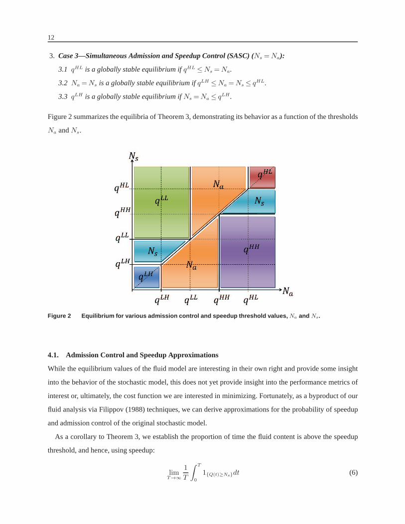
Figure 2 summarizes the equilibria of Theorem 3, demonstrating its behavior as a function of the thresholds

Na andNs.

Figure 2 Equilibrium for various admission control and spee dup threshold values, Na and Ns.

4.1. Admission Control and Speedup Approximations

While the equilibrium values of the fluid model are interesting in their own right and provide some insight

into the behavior of the stochastic model, this does not yet provide insight into the performance metrics of

interest or, ultimately, the cost function we are interested in minimizing. Fortunately, as a byproduct of our

fluid analysis via Filippov (1988) techniques, we can deriveapproximations for the probability of speedup

and admission control of the original stochastic model.

As a corollary to Theorem 3, we establish the proportion of time the fluid content is above the speedup

threshold, and hence, using speedup:

limT→∞

1

T

∫ T

0

1{Q(t)≥Ns}dt (6)

13

and admission control threshold, and hence, using admission control:

limT→∞

1

T

∫ T

0

1{Q(t)≥Na}dt (7)

We formally provide the statement for the ACF case (Na < Ns) and note that the other two cases follow

similarly and will be summarized later in Table 1.

Corollary 1 Under Assumption 1 and ACF case (Na <Ns), the proportion of time the fluid process is above

the admission control threshold is given by:

limT→∞

1

T

∫ T

0

1{Q(t)≥Na}dt=

0, qHL ≤Na;λH−µL(N∧Na)

λH−λL, qLL ≤Ns ≤ q

HL;1, Na ≤ q

LL ≤Ns;1, Ns ≤ q

LH ;1, qLH ≤Ns ≤ q

LL.

(8)

Similarly, the proportion of time the fluid process is above the speedup control threshold is given by:

limT→∞

1

T

∫ T

0

1{Q(t)≥Ns}dt=

0, qHL ≤Na;0, qLL ≤Ns ≤ q

HL;0, Na ≤ q

LL ≤Ns;λL−µL(N∧Ns)

(µH−µL)(N∧Ns), qLH ≤Ns ≤ q

LL.1, Ns ≤ q

LH .

(9)

Consequently, these values can provide approximations forthe probability that speedup and admission

control are used in our original stochastic system from Section 2. In particular, we approximate the following

probabilities of our original stochastic model as:

P (Speedup) = P (Q≥Ns)≈ limT→∞

1

T

∫ T

0

1{Q(t)≥Ns}dt (10)

P (Admission Control) = P (Q≥Na)≈ limT→∞

1

T

∫ T

0

1{Q(t)≥Na}dt (11)

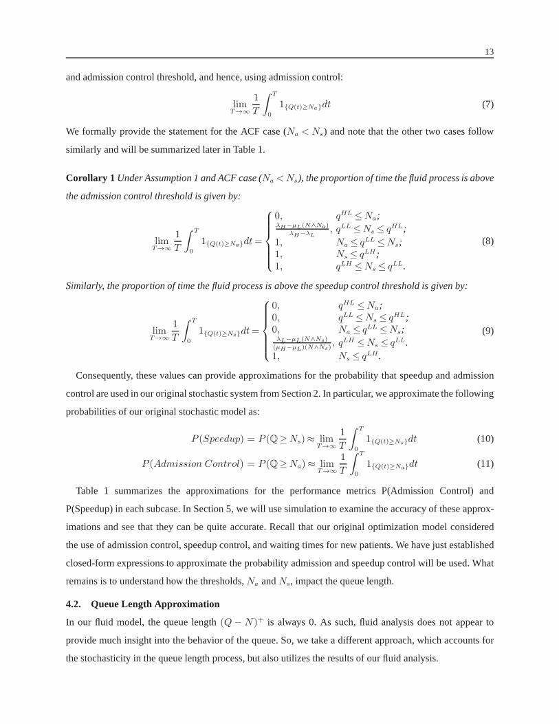
Table 1 summarizes the approximations for the performance metrics P(Admission Control) and

P(Speedup) in each subcase. In Section 5, we will use simulation to examine the accuracy of these approx-

imations and see that they can be quite accurate. Recall thatour original optimization model considered

the use of admission control, speedup control, and waiting times for new patients. We have just established

closed-form expressions to approximate the probability admission and speedup control will be used. What

remains is to understand how the thresholds,Na andNs, impact the queue length.

4.2. Queue Length Approximation

In our fluid model, the queue length(Q − N)+ is always 0. As such, fluid analysis does not appear to

provide much insight into the behavior of the queue. So, we take a different approach, which accounts for

the stochasticity in the queue length process, but also utilizes the results of our fluid analysis.

14

Case P(Admission Control) P(Speedup)

(1)

AC

F

1.1 0 01.2 λH−µL(N∧Na)

λH−λL0

1.3 1 01.4 1 λL−µL(N∧Ns)

(µH−µL)(N∧Ns)

1.5 1 1

(2)

SC

F

2.1 0 02.2 0 λH−µL(N∧Ns)

(µH−µL)(N∧Ns)

2.3 0 12.4 λH−µH (N∧Na)

λH−λL1

2.5 1 1

(3)

SA

SC 3.1 0 0

3.2 λH−µL(N∧Na)

λH−λL−(µL−µH )(N∧Na)

λH−µL(N∧Na)

λH−λL−(µL−µH )(N∧Na)

3.3 1 1Table 1 Performance level approximations for the probabili ty of speedup and admission control in each

subcase. The approximations come from the derived proporti on of time the fluid content is about

the speedup and/or admission control thresholds.

We start by considering the extreme cases where the fluid analysis suggests that speedup and/or admission

control is always or never used. In such a scenario, it is conceivable that very limited information is lost

by ignoring the change in dynamics due to the thresholds. As an example, consider the ACF case where

qHL ≤Na (case 1.1). In this case, the fluid analysis suggests that neither speedup or admission control is

ever used. If this were truly the case, the system would evolve as an M/M/N queue with arrival rateλ= λH

and service rateµ= µL. Using standard approaches, we can then get an approximation for the queue length

given by the analysis of this M/M/N queue. Via a similar argument, we could do the same in case 1.3 with

λ= λH andµ= µH .

When the equilibrium is on a control threshold (eitherNa or Ns), it is certain that the dynamics are

changing due to the threshold. In fact, they are changing very rapidly, so that the fluid content remains on the

threshold boundary. In these cases (1.2, 1.4, 2.2, 2.4, and 3.2), we still use an M/M/N queue to approximate

the dynamics; however, the stateindependentarrival and departure rates will be given by the average arrival

and departure rates as approximated by the fluid analysis. Hence, for all cases we will consider the following

arrival and departure rates:λ= P(Admission Control)× λL + (1− P(Admission Control))× λH andµ=

P(Speedup)×µH +(1−P(Speedup))×µL, where P(Admission Control) and P(Speedup) are given by our

fluid analysis as summarized in Table 1.

Using the analysis of an M/M/N queue, with arrival rateλ and departure rateµ, can provide very reason-

able estimates of the simulated queue length of our state-dependent queueing system when whenNa andNs

are smaller thanN . However, when both of the thresholds are larger thanN , we find that the approximation

via the M/M/N queue overestimates the queue length. That is because the change in arrival and service

15

rates “push” the derivative (Q) down and decrease the queue length. To capture this strong push, we instead

use an M/M/N/K queue (a loss model), whereK =min{Na,Ns}, whenmin{Na,Ns} ≥N andK =N ,

otherwise. The loss model queue length is derived by solvingthe local balance equations:

πi =1

i!

(

µ

λ

)−i

π0 0≤ i≤N

πi =NN

N !

(

λ

Nµ

)i

π0 N < i≤K

π0 =

N∑

i=0

1

i!

(

µ

λ

)−i

+K∑

i=N+1

NN

N !

(

λ

Nµ

)i

−1

. (12)

Finally, we have that

E[

[Q−N ]+]

≈E[QueueM/M/N/K ] =K∑

i=N

(i−N)πi.

In Section 5, we will see that this approximation works very well. To provide some intuition as to why

this seems to provide a very accurate approximation, we consider the impact of the finite buffer in the loss

model. When there areK jobs in an M/M/N/K queue, the loss of any new job ‘forces’ the system away from

this boundary. The speedup and/or admission control thresholds have a similar effect. When the number

of patients in the system crosses one of these thresholds, the change in dynamics due to increased service

rate and/or decreased arrival rate also ‘forces’ the systemdown and away from that threshold. When these

thresholds are less thanN , this strong push is active prior to a queue forming (i.e. whenQ<N ). Since we

are interested in examining the queue length,Q > N , ignoring the change in dynamics before the queue

forms does not degrade our approximation. If we were interested in approximating the precise distribution

of patients in the system, it is likely the M/M/N/K approximation is too coarse; however, it seems to work

quite well in approximating the mean queue length.

Remark 3 One can utilize the derived approximations for the mean queue length and the probability of

admission control and speedup to do performance analysis given thresholdsNa andNs. Moreover, it is

possible to determine a feasible set ofNa andNs such that various constraints on these performance mea-

sures are satisfied. For example, if hospital management seta limit on the proportion of time that admission

control is utilized, our approximations would provide a setof thresholds to satisfy such a constraint.

4.3. Cost Minimization

Now that we have derived approximations for the different performance metrics, we are in position to

consider our original optimization problem from (1). Because we’ve established the optimality of threshold

policies in Section 3, our optimization problem can be reduced to:

minNa,Ns

{h(E[

[Q−N ]+]

) + P (Q≥Na)φ(λL)+P (Q<Na)φ(λH)

16

+ P (Q≥Ns)ξ(µH)+P (Q<Ns)ξ(µL)}. (13)

With our approximations from Sections 4.1 and 4.2, we now have closed form expressions for approxima-

tions to the optimization problem in (13). Without loss of generality, we setφ(λH) = 0 andξ(µL) = 0,

so there is no cost associated with the nominal system arrival and service rates. We also consider a linear

function for the queue length costs. Hence, our optimization model is:

minNa,Ns

{cwE[

[Q−N ]+]

+ caP (Q≥Na)+ csP (Q≥Ns)} (14)

wherecw is the per-patient waiting cost rate,ca = φ(λL) is the cost rate for admission control, andcs =

ξ(µH) is the cost rate for speedup.

Observation 1 Using the approximations in Section 4.1 and 4.2 we find regimes in which our approxima-

tions suggest the cost in(14) to be zero. In particular, this occurs in cases 1.1, 2.1 and 3.1. Thus, the cost

(14) is zero when:

qHL ≤Na ∧Ns ≤N.

This implies that it always ‘optimal’ to use at least one formof congestion controlbeforea queue builds

regardlessof the exact system parameters; a zero cost solution will never have bothNa,Ns >N .

There has been some evidence that hospitals do use speedup and/or admission controlbeforereaching full

capacity (e.g. Kim et al. (2014) and Kc and Terwiesch (2012)). However, in other cases, such as ambulance

diversion, admission control is not used until a queue builds (Allon et al. 2013).

As we will see in Section 5.2, one must be prudent with how to select between these seemingly zero-cost

solutions.

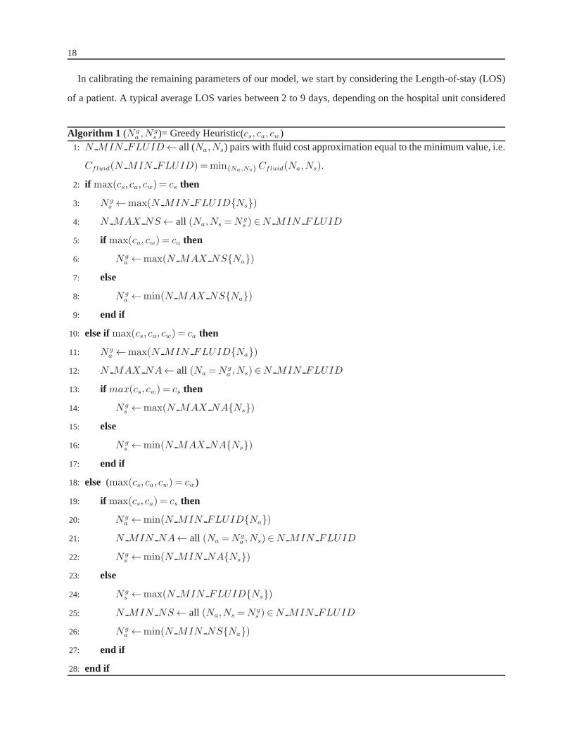
4.3.1. A Greedy Heuristic We suggest the followingGreedyheuristic to select the (Na,Ns) amongst

the potentially numerous solutions with the minimal approximated cost as indicated in Observation 1. In

general, this heuristic prioritizes the use of the speedup and admission control in decreasing order of the

cost measure. In order to ensure the costs are comparable, weuse normalized costs. While, P(Speedup) and

P(Admission Control) are naturally normalized to the range[0,1], the range ofE[QueueM/M/N/K ] can vary

dramatically. Hence, we normalize the waiting costs by dividing them by the maximum expected queue

length, denoted byQmax, which is obtained when speedup or admission control are never used.

The Greedy heuristic then selects among the potentially numerous solutions with approximated zero

costs. For example, if speedup has the highest costs (cs is maximal) thenNs should be as large as possible.

This implies that only admission control is used; additionally, in light of Observation 1, we know thatqHL ≤

Na ≤N . The value ofNa will then be selected based on the relative costs between admission control and

17

waiting. Under a similar argument, if admission control is most expensive (ca is maximal) thenNa should

be as large as possible andqHL ≤Ns ≤N . Finally, if waiting is most costly (cw/Qmax is maximal), thenNa

andNs should be as small as possible. The Greedy heuristic is defined more formally by the pseudo-code

in Algorithm 1. In Section 5.2, we will use simulation to examine how well such an approach performs.

5. Numerical Results

In this section we examine the accuracy of our approximations. Subsection 5.1 presents the accuracy of

the fluid approximations forP (Speedup), P (AdmissionControl) and the M/M/N/K model approxima-

tion for E[Queue]. Assuming these are reasonably accurate, the next step is toconsider the performance

of decisions which are optimized over these approximations—this is presented in Subsection 5.2. In our

numeric analysis, we consider two system sizes: a small system representing an ICU setting and a large

system representing the entire hospital. As our approximations are based on fluid analysis, we expect that

they will be more accurate for the larger system.

5.1. Numerical Results: Performance Measure

We calibrate the parameters of our model according to typical healthcare environments. We used publicly

available data from State of California Office of Statewide Health Planning & Development (2010-2011)

which keeps track of all hospitals in California. We only considered short-term, acute hospitals with 24

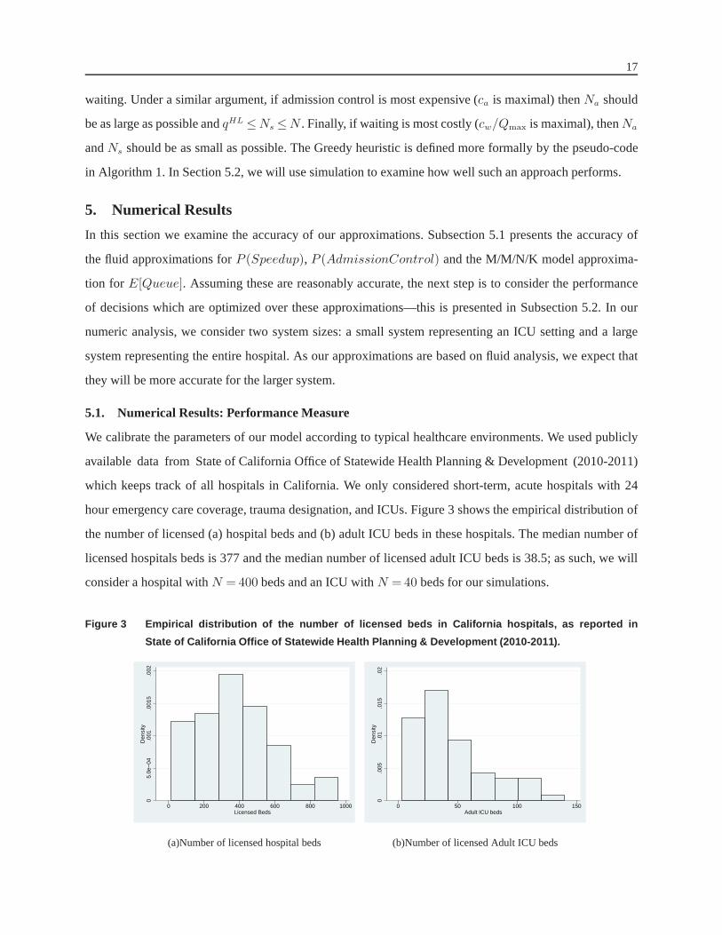
hour emergency care coverage, trauma designation, and ICUs. Figure 3 shows the empirical distribution of

the number of licensed (a) hospital beds and (b) adult ICU beds in these hospitals. The median number of

licensed hospitals beds is 377 and the median number of licensed adult ICU beds is 38.5; as such, we will

consider a hospital withN = 400 beds and an ICU withN =40 beds for our simulations.

Figure 3 Empirical distribution of the number of licensed be ds in California hospitals, as reported in

State of California Office of Statewide Health Planning & Dev elopment (2010-2011).

05.

0e−

04.0

01.0

015

.002

Den

sity

0 200 400 600 800 1000Licensed Beds

(a)Number of licensed hospital beds

0.0

05.0

1.0

15.0

2D

ensi

ty

0 50 100 150Adult ICU beds

(b)Number of licensed Adult ICU beds

18

In calibrating the remaining parameters of our model, we start by considering the Length-of-stay (LOS)

of a patient. A typical average LOS varies between 2 to 9 days,depending on the hospital unit considered

Algorithm 1 (Nga ,N

gs )= Greedy Heuristic(cs, ca, cw)

1: N MIN FLUID← all (Na,Ns) pairs with fluid cost approximation equal to the minimum value, i.e.

Cfluid(N MIN FLUID) =min{Na,Ns}Cfluid(Na,Ns).

2: if max(cs, ca, cw) = cs then

3: Ngs ←max(N MIN FLUID{Ns})

4: N MAX NS← all (Na,Ns =Ngs )∈N MIN FLUID

5: if max(ca, cw) = ca then

6: Nga ←max(N MAX NS{Na})

7: else

8: Nga ←min(N MAX NS{Na})

9: end if

10: else ifmax(cs, ca, cw) = ca then

11: Nga ←max(N MIN FLUID{Na})

12: N MAX NA← all (Na =Nga ,Ns)∈N MIN FLUID

13: if max(cs, cw) = cs then

14: Ngs ←max(N MAX NA{Ns})

15: else

16: Ngs ←min(N MAX NA{Ns})

17: end if

18: else (max(cs, ca, cw) = cw)

19: if max(cs, ca) = cs then

20: Nga ←min(N MIN FLUID{Na})

21: N MIN NA← all (Na =Nga ,Ns)∈N MIN FLUID

22: Ngs ←min(N MIN NA{Ns})

23: else

24: Ngs ←max(N MIN FLUID{Ns})

25: N MIN NS← all (Na,Ns =Ngs )∈N MIN FLUID

26: Nga ←min(N MIN NS{Na})

27: end if

28: end if

19

(see, for example, Table 3 in de Bruin et al. (2010)). Hence, we chose a lower value of 3 hospital days

as the LOS under speedup and 5 days as the LOS under ‘unstressed’, nominal conditions. The arrival

rates are chosen in order to have approximately 20% bed turnover per day under high arrival rates and

10% under low arrival rates. For our simulations, we use the following parameters for an ’ICU’ (i.e. small

system):λL = 4, λH =7.5, µL = 0.2, µH = 0.286,N = 40. For an average sized hospital (i.e. large system),

we use:λL = 50, λH = 78, µL = 0.2, µH = 0.286,N = 400. Note that the parameters chosen here satisfy

Assumption 1, so that the system is stable irrespective of whether or not speedup and/or admission control

are used.

Figure 4 presents the performance metrics given by our approximations and simulation results for the

large system (left column) and small system (right column) as we vary the thresholdsNa andNs1. These

figures are meant to illustrate the typical behavior and effect of the control thresholds. The results are very

similar across all combinations of the thresholds,Na andNs.

As expected, the approximations are more accurate for the large system. Still, they can be quite accurate

for the small system as well. We observe that the approximations are very good in most cases. Some gaps

can be observed when speedup and/or admission control is used for some (but small) proportion of the time

(e.g. 5–10%) or when it is used most (but not all) of the time (e.g. 90–95%). This is more pronounced in the

small system. In such situations, the fluid approximations for P(Speedup) and/or P(Admission Control) are

not very accurate. This can result in degradation in the queue length approximation. For example, in Fig-

ure 5(d), the approximation for the probability of admission control is 0, while the simulation suggests the

true probability is around 10%. Because our queue length approximation uses the probability of admission

control to derive an ‘effective’ arrival rate,λ, poor estimates for P(Admission Control) also result in poor

estimates forE[Q]. This is not always the case. In Figure 5(f), the approximation of P(speedup) under esti-

mates the simulated value. However, in this case, the expected queue length is effectively 0 in the simulation

and via our approximation.

5.2. Numerical Results: Approximation-Based Cost Minimization

As the performance metric approximations appear to be quiteaccurate, the next step is to consider the

performance of policies resulting from solving an optimization problem based on them. The normalization

factorQmax in our examples are: in the large systemQmax = 19.7, and in the small systemQmax = 8.9. Here

we findNa andNs which minimize the approximated costs and use simulation tocompare the resulting cost

to the minimum cost achieved via exhaustive search over manyNa andNs combinations. We also consider

a number of benchmarks for comparison:

1 Note that, due to numeric issues, in order to calculate the expected queue length for large systems we used Stirling’s formula(

i!∼(

ie

)i√2πi

)

(Hazewinkel 2001) to calculateE[Queue].

20

Figure 4 Approximation vs. simulation results as a function of the Speedup threshold (Ns) for some fixed

Admission threshold (Na) values

Large (Hospital) system withN = 400 Small (ICU) system withN = 40

0 100 200 300 400 500 6000

10

20

E[Q

]N

a = 550

0 100 200 300 400 500 6000

0.5

1

P(A

dm

issio

n)

0 100 200 300 400 500 6000

0.5

1

Ns

P(S

peedup)

(a)Na = 550

0 20 40 60 80 1000

2.5

5

E[Q

]

Na = 65

0 20 40 60 80 1000

0.5

1

P(A

dm

issio

n)

0 20 40 60 80 1000

0.5

1

Ns

P(S

peedup)

(b) Na =65

0 100 200 300 400 500 6000

0.5

1

E[Q

]

Na = 400

0 100 200 300 400 500 6000

0.5

1

P(A

dm

issio

n)

0 100 200 300 400 500 6000

0.5

1

Ns

P(S

peedup)

(c)Na = 400

0 20 40 60 80 1000

0.5

1E

[Q]

Na = 40

0 20 40 60 80 1000

0.5

1

P(A

dm

issio

n)

0 20 40 60 80 1000

0.5

1

Ns

P(S

peedup)

(d)Na = 40

0 100 200 300 400 500 6000

0.5

1

E[Q

]

Na = 225

0 100 200 300 400 500 6000

0.5

1

P(A

dm

issio

n)

0 100 200 300 400 500 6000

0.5

1

Ns

P(S

peedup)

Simulation

Approximation

(e)Na = 225

0 20 40 60 80 1000

0.5

1

E[Q

]

Na = 30

0 20 40 60 80 1000

0.5

1

P(A

dm

issio

n)

0 20 40 60 80 1000

0.5

1

Ns

P(S

peedup)

(f) Na =30

• Neveruse speedup or admission control:Na =Ns =∞

• Use speedup and admission control as soon asall beds are filled: Na =Ns =N

21

• Always use speedup or admission control:Na =Ns =0

We derive the optimal performance via exhaustive search; for the large system we checked integer thresh-

olds between 0 to 700 in jumps of 52, and for the small systems we search all combinations of integer

thresholds between 0 to 100. The fluid approximation is derived by solving the optimization problem in

(14) using the approximations for P(Speedup), P(AdmissionControl) and E[Queue] as given in Sections

4.1 and 4.2.

Figure 5 Distribution of simulation costs when approximate d costs equal 0 (large system, scenario 11).

!"

#"

$"

%"

&"

'"

("

)"

*"

+"

#!"

#"

$#"

&#"

(#"

*#"

#!#"

#$#"

#&#"

#(#"

#*#"

$!#"

$$#"

$&#"

$(#"

$*#"

%!#"

%$#"

%&#"

%(#"

!"#$%

&"'($)"*%+(,-./%

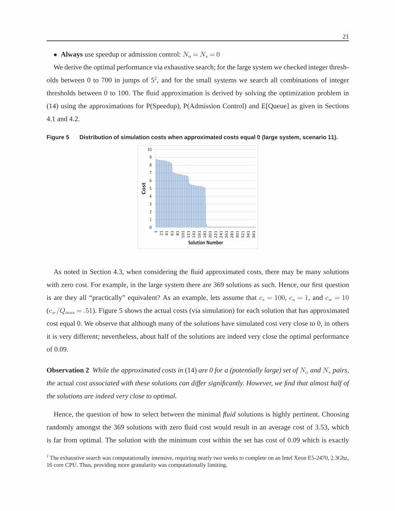
As noted in Section 4.3, when considering the fluid approximated costs, there may be many solutions

with zero cost. For example, in the large system there are 369solutions as such. Hence, our first question

is are they all “practically” equivalent? As an example, lets assume thatcs = 100, ca = 1, andcw = 10

(cw/Qmax = .51). Figure 5 shows the actual costs (via simulation) for each solution that has approximated

cost equal 0. We observe that although many of the solutions have simulated cost very close to 0, in others

it is very different; nevertheless, about half of the solutions are indeed very close the optimal performance

of 0.09.

Observation 2 While the approximated costs in(14)are 0 for a (potentially large) set ofNa andNs pairs,

theactualcost associated with these solutions can differ significantly. However, we find that almost half of

the solutions are indeed very close to optimal.

Hence, the question of how to select between the minimalfluid solutions is highly pertinent. Choosing

randomly amongst the 369 solutions with zero fluid cost wouldresult in an average cost of 3.53, which

is far from optimal. The solution with the minimum cost within the set has cost of 0.09 which is exactly

2 The exhaustive search was computationally intensive, requiring nearly two weeks to complete on an Intel Xeon E5-2470, 2.3Ghz,16 core CPU. Thus, providing more granularity was computationally limiting.

22

equal to the optimal value. Yet, finding this solution requires simulating all 369 zero fluid cost solutions.

Although this is not as extensive as the run that is required for an exhaustive search, it is still computationally

intensive. With this in mind, we consider the Greedy heuristic presented in Section 4.3. We next examine

its performance for different cost scenarios.

Table 2 summarizes the cost scenarios we consider. We chose these scenarios in order to examine what

happens where the costs have the same order of magnitude (scenarios 1–6), but still different order of

importance; or when they are of different orders of magnitude (scenarios 7–12), highly emphasizing one

measure in particular.

Cost ScenarioSpeedup Controlcs Admission Controlca Waiting Cost (before normalization)cw1 1 2 32 1 3 23 2 1 34 2 3 15 3 1 26 3 2 17 1 10 1008 1 100 109 10 1 10010 10 100 111 100 1 1012 100 10 1

Table 2 Cost parameters for different cost minimization sce narios.

Tables 3 and 4 present the performance of the different strategies, for the various cost scenarios. The first

thing we note is therobustnessof the optimal solution. The left column—optimal—presents the minimal

solution found using exhaustive search for each cost scenario. Analyzing this solution, we note that the

minimal cost is robust. For example, for the large system there are between 8–14 solutions within 5% of

the minimal one, and 57–105 solutions within 10% of it. (The numbers for the small systems are 6–176

solutions within 5% and 15–477 within 10% of the optimal performance). Note also that the “optimal”

value was found by simulation; hence, numerical errors may indicate that one of the close solutions is

indeed the optimal one. Under thevia Fluid Approximationcolumn we present the minimal simulated cost

within the set of zero-value fluid solutions (Min), the average performance of these solutions (Avg), and the

performance of the solution selected by the Greedy heuristic (Greedy). We make the following observations:

1. In most cases, the optimal value is within the set of zero fluid cost solutions.

2. The difference between the minimal performance of the zero fluid cost solution set and the optimal one

is very small (often times it is 0).

23

3. The average cost of the zero fluid cost solution set may be quite far from optimal; hence, it is important

to choose wisely within this range.

4. The Greedy heuristic is very close to optimal, achieving in most cases the minimal performance. Thus,

prioritizing admission control and/or speedup based on relative costs can be very cost-effective.

The last three columns show the performance of the benchmarkpolicies: Never, Always, and All beds

filled. We see that the simple benchmarks fail dramatically in all scenarios; the only reasonable one is the

“All beds filled” policy. Still, while the Greedy heuristic failed only in one scenario (in scenario 9 of the

small system), the “All beds filled” performs well only for large systems where costs are close in magnitude

(Scenarios 1–6); even then, it never achieves the optimal cost. We surmise that using the combination of

the fluid approximation with the Greedy heuristic is a very good way to find a solution with near optimal

performance.

PolicyCost Optimal via Fluid Never: Always: All beds filled:

Scenario Approximations Na =Ns =∞ Na =Ns =0 Na =Ns =NMin Avg Greedy

1 0.07 0.07∗ 0.12 0.07∗ 3.06 3.00 0.092 0.06 0.06∗ 0.16 0.06∗ 2.04 4.00 0.123 0.08 0.08∗ 0.12 0.08∗ 3.06 3.00 0.094 0.10 0.11 0.19 0.11 1.02 5.00 0.155 0.07 0.07∗ 0.15 0.07∗ 2.04 4.00 0.126 0.12 0.13 0.19 0.13 1.02 5.00 0.15

7 0.10 0.10∗ 0.66 0.10∗ 101.84 11.00 0.458 0.07 0.07∗ 4.17 0.11 10.18 101.00 3.039 0.10 0.10∗ 0.60 0.11 101.84 11.00 0.4510 0.35 0.51 446 0.52 1.02 110.00 3.2911 0.09 0.09∗ 3.53 0.11 10.18 101.00 3.0312 0.40 0.61 3.88 0.61 1.02 110.00 3.29

Bold font indicates the method that got the minimal cost value;∗ indicates optimal costsTable 3 Large system: Performance of different strategies f or cost scenarios 1–12.

5.3. Cost Misspecification: Robustness of Proposed Greedy Policy

We also consider the robustness of our proposed greedy heuristic to miss-estimates in the cost parameters:

cw, ca andcs. Certainly, if the optimization is done over costs which areincorrectly specified, the resulting

policy will be suboptimal. The question is how much worse will the performance be. Additionally, since we

know the greedy heuristic is suboptimal, how will its performance be impacted by such misspecification?

To examine this, we consider the thresholds,Na andNs, selected under the Greedy Heuristic and Optimal

Policy when the costs are misspecified by plus or minus 10%, 20%, 30%, 40%, and 50%. The thresholds

24

PolicyCost Optimal via Fluid Never: Always: All beds filled:

Scenario Approximations Na =Ns =∞ Na =Ns =0 Na =Ns =NMin Avg Greedy

1 0.24 0.24∗ 0.32 0.26 2.76 3.00 0.292 0.22 0.22∗ 0.40 0.22∗ 1.84 4.00 0.373 0.20 0.20∗ 0.32 0.20∗ 2.76 3.00 0.294 0.29 0.34 0.47 0.35 0.92 5.00 0.455 0.18 0.18∗ 0.40 0.19 1.84 4.00 0.376 0.27 0.32 0.47 0.32 0.92 5.00 0.45

7 0.62 0.97 2.73 1.42 91.80 11.00 1.548 0.38 0.39 9.29 0.40 9.27 101.00 9.129 0.37 0.56 2.73 1.42 91.80 11.00 1.5410 0.69 1.56 9.95 1.59 1.01 110.00 9.8711 0.26 0.26∗ 9.30 0.26∗ 9.27 101.00 9.1212 0.67 1.53 9.96 1.54 1.01 110.00 9.87

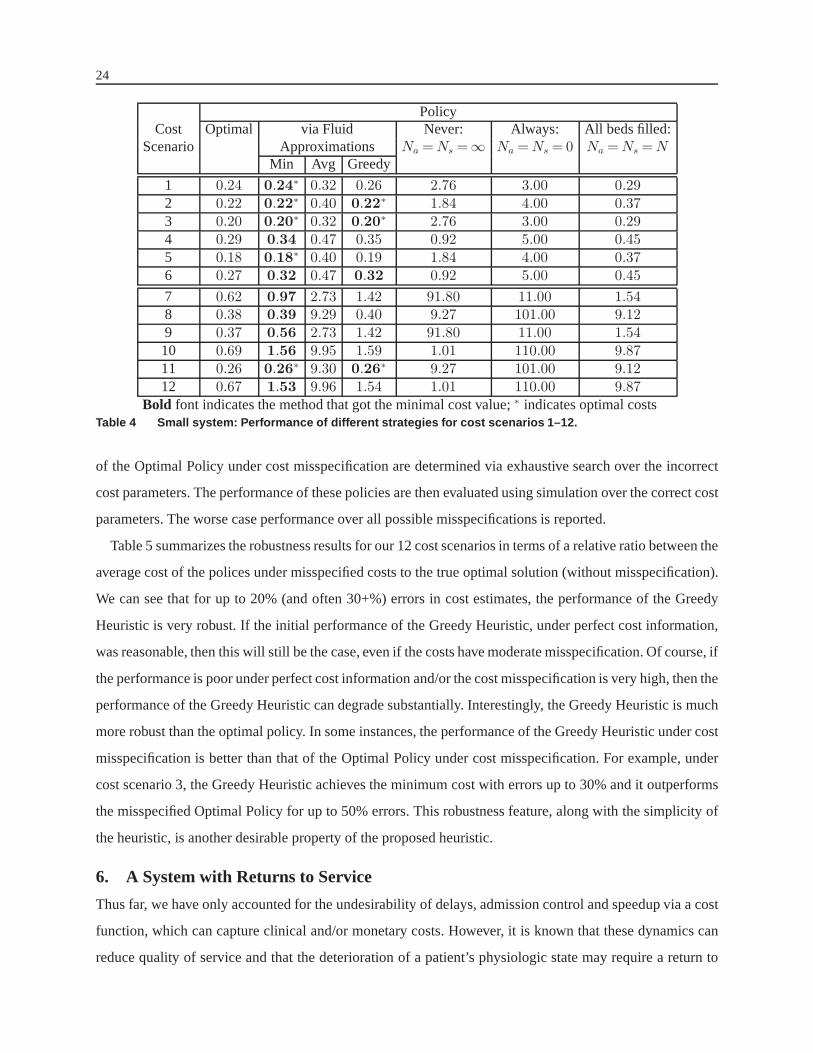
Bold font indicates the method that got the minimal cost value;∗ indicates optimal costsTable 4 Small system: Performance of different strategies f or cost scenarios 1–12.

of the Optimal Policy under cost misspecification are determined via exhaustive search over the incorrect

cost parameters. The performance of these policies are thenevaluated using simulation over the correct cost

parameters. The worse case performance over all possible misspecifications is reported.

Table 5 summarizes the robustness results for our 12 cost scenarios in terms of a relative ratio between the

average cost of the polices under misspecified costs to the true optimal solution (without misspecification).

We can see that for up to 20% (and often 30+%) errors in cost estimates, the performance of the Greedy

Heuristic is very robust. If the initial performance of the Greedy Heuristic, under perfect cost information,

was reasonable, then this will still be the case, even if the costs have moderate misspecification. Of course, if

the performance is poor under perfect cost information and/or the cost misspecification is very high, then the

performance of the Greedy Heuristic can degrade substantially. Interestingly, the Greedy Heuristic is much

more robust than the optimal policy. In some instances, the performance of the Greedy Heuristic under cost

misspecification is better than that of the Optimal Policy under cost misspecification. For example, under

cost scenario 3, the Greedy Heuristic achieves the minimum cost with errors up to 30% and it outperforms

the misspecified Optimal Policy for up to 50% errors. This robustness feature, along with the simplicity of

the heuristic, is another desirable property of the proposed heuristic.

6. A System with Returns to Service

Thus far, we have only accounted for the undesirability of delays, admission control and speedup via a cost

function, which can capture clinical and/or monetary costs. However, it is known that these dynamics can

reduce quality of service and that the deterioration of a patient’s physiologic state may require a return to

25

Relative performance of Relative performance of‘Optimal Policy’ Greedy Heuristic

Cost with cost misspecifications with cost misspecificationsScenario 0 % 10 % 20 % 30 % 40 % 50 % 0% 10 % 20 % 30 % 40 % 50 %

1 1.000 1.001 1.001 1.399 1.399 2.055 1.019 1.019 1.019 1.019 2.055 2.0552 1.000 1.000 1.000 1.074 1.074 1.074 1.018 1.018 1.018 1.018 1.018 3.1473 1.000 1.000 1.225 1.539 1.716 1.716 1.000 1.000 1.000 1.000 1.565 1.5654 1.000 1.027 1.027 1.633 1.815 1.815 1.043 1.043 1.043 1.815 1.815 1.8155 1.000 1.000 1.000 1.000 1.717 2.282 1.000 1.000 1.000 1.000 1.000 1.0006 1.000 1.102 1.180 1.292 1.292 1.346 1.046 1.046 1.046 1.312 1.312 1.312

7 1.000 1.007 1.048 1.066 1.066 1.402 1.045 1.045 1.045 1.045 5.615 5.6158 1.000 1.000 1.000 1.000 1.000 1.150 1.456 1.456 1.456 1.456 1.456 1.4569 1.000 1.002 1.007 1.025 1.199 1.297 1.041 1.041 1.041 1.041 5.352 5.35210 1.000 1.000 1.085 1.140 1.269 1.343 1.479 1.479 1.479 1.479 1.479 1.47911 1.000 1.000 1.000 1.000 1.003 1.309 1.309 1.309 1.309 1.309 1.309 1.30912 1.000 1.016 1.045 1.045 1.215 1.257 1.535 1.535 1.535 1.535 1.535 1.535

Table 5 Large system: Robustness of greedy policy—Relative performance of Optimal Policy and Greedy

Heuristic when cost parameters are misspecified to the true m inimum cost.

service. A common quality measure used in practice is readmission rates. Using simulation, we examine

an extended model that incorporates patients’ readmissions explicitly, and use our original model (without

readmissions) to determine policies which minimize the readmission rate for the extended model.

To incorporate readmissions, we assume that waiting for service and/or using speedup or admission

control increases the likelihood of readmission. Without loss of generality, we assume the readmission risk

to be 0 if neither speedup or admission control are used (i.e.µ= µL, λ= λH) and the new patient does not

have to wait to begin service (Qt <N wheret is the patient’s arrival time). If a patient would have arrived

under the nominal arrival rate,λH , but was blocked due to admission control, this patient may return to

service with probabilitypRλ after some time which is exponentially distributed with mean 1/δa. Similarly, if

a patient is discharged under speedup, his probability of a return to service increases bypRµ ; he returns after

1/δs units of time (on average). If the patient arrives to the system withQ patients waiting in front of him

for service, his probability of return to service increasesby pRw× (Q−N)+, wherepRw× (Qmax−N)+≪ 1.

Thus, if a patient arrives withq patients in the system and then is discharged under speedup,his probability

of return to service ispRµ + pRw × (q−N)+. On the other hand, if the same patient is discharged under the

nominal service rate, his probability of return to service is pRw × (q−N)+. We simulate such a model for

eachNa andNs combination with 40 iterations of 100 days each3. We then use exhaustive search to find

the thresholds,Na andNs, which minimize the readmission rate.

3 Given the computational complexity of this simulation–we must keep track of the number of customers in the system upon arrivalfor each customer–the number of repetitions was limited to 40.

26

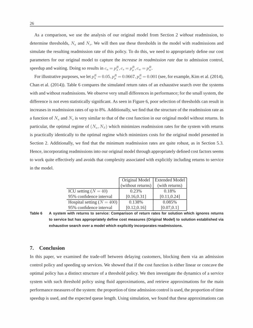
As a comparison, we use the analysis of our original model from Section 2without readmission, to

determine thresholds,Na andNs. We will then use these thresholds in the model with readmissions and

simulate the resulting readmission rate of this policy. To do this, we need to appropriately define our cost

parameters for our original model to capture theincrease in readmission ratedue to admission control,

speedup and waiting. Doing so results inca = pRλ , cs = pRµ , cw = pRw.

For illustrative purposes, we letpRλ = 0.05, pRµ = 0.0667, pRw = 0.001 (see, for example, Kim et al. (2014),

Chan et al. (2014)). Table 6 compares the simulated return rates of an exhaustive search over the systems

with and without readmissions. We observe very small differences in performance; for the small system, the

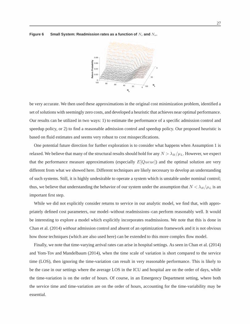
difference is not even statistically significant. As seen inFigure 6, poor selection of thresholds can result in

increases in readmission rates of up to 8%. Additionally, wefind that the structure of the readmission rate as

a function ofNa andNs is very similar to that of the cost function in our original model without returns. In

particular, the optimal regime of(Na,NS) which minimizes readmission rates for the system with returns

is practically identically to the optimal regime which minimizes costs for the original model presented in

Section 2. Additionally, we find that the minimum readmission rates are quite robust, as in Section 5.3.

Hence, incorporating readmissions into our original modelthrough appropriately defined cost factors seems

to work quite effectively and avoids that complexity associated with explicitly including returns to service

in the model.

Original Model Extended Model(without returns) (with returns)

ICU setting (N = 40) 0.23% 0.18%95% confidence interval [0.16,0.31] [0.11,0.24]Hospital setting (N = 400) 0.138% 0.085%95% confidence interval [0.12,0.16] [0.07,0.1]

Table 6 A system with returns to service: Comparison of retur n rates for solution which ignores returns

to service but has appropriately define cost measures (Origi nal Model) to solution established via

exhaustive search over a model which explicitly incorporat es readmissions.

7. Conclusion

In this paper, we examined the trade-off between delaying customers, blocking them via an admission

control policy and speeding up services. We showed that if the cost function is either linear or concave the

optimal policy has a distinct structure of a threshold policy. We then investigate the dynamics of a service

system with such threshold policy using fluid approximations, and retrieve approximations for the main

performance measures of the system: the proportion of time admission control is used, the proportion of time

speedup is used, and the expected queue length. Using simulation, we found that these approximations can

27

Figure 6 Small System: Readmission rates as a function of Ns and Na.

020

4060

80100

0

50

100

0

0.02

0.04

0.06

0.08

Ns

Na

Retu

rn P

rob

ab

ilit

y

be very accurate. We then used these approximations in the original cost minimization problem, identified a

set of solutions with seemingly zero costs, and developed a heuristic that achieves near optimal performance.

Our results can be utilized in two ways: 1) to estimate the performance of a specific admission control and

speedup policy, or 2) to find a reasonable admission control and speedup policy. Our proposed heuristic is

based on fluid estimates and seems very robust to cost misspecifications.

One potential future direction for further exploration is to consider what happens when Assumption 1 is

relaxed. We believe that many of the structural results should hold for anyN >λH/µL. However, we expect

that the performance measure approximations (especiallyE[Queue]) and the optimal solution are very

different from what we showed here. Different techniques are likely necessary to develop an understanding

of such systems. Still, it is highly undesirable to operate asystem which is unstable under nominal control;

thus, we believe that understanding the behavior of our system under the assumption thatN <λH/µL is an

important first step.

While we did not explicitly consider returns to service in our analytic model, we find that, with appro-

priately defined cost parameters, our model–without readmissions–can perform reasonably well. It would

be interesting to explore a model which explicitly incorporates readmissions. We note that this is done in

Chan et al. (2014)withoutadmission control and absent of an optimization framework and it is not obvious

how those techniques (which are also used here) can be extended to this more complex flow model.

Finally, we note that time-varying arrival rates can arise in hospital settings. As seen in Chan et al. (2014)

and Yom-Tov and Mandelbaum (2014), when the time scale of variation is short compared to the service

time (LOS), then ignoring the time-variation can result in very reasonable performance. This is likely to

be the case in our settings where the average LOS in the ICU andhospital are on the order of days, while

the time-variation is on the order of hours. Of course, in an Emergency Department setting, where both

the service time and time-variation are on the order of hours, accounting for the time-variability may be

essential.

28

ReferencesAdusumilli, K. M., J. J. Hasenbein. 2010. Dynamics admission and service rate control of a queue.Queueing Systems

66131–154.

Allon, G., S. Deo, W. Lin. 2013. The impact of hospital size and occupancy of hospital on the extent of ambulance

diversion: Theory and evidence.Operations Research61(3) 544–562.

Anand, K., M. F. Pac, S. Veeraraghavan. 2010. Quality-speedconundrum: Tradeoffs in customer-intensive services.

Management Science5740–56.

Ata, B., S. Shneorson. 2006. Dynamic control of an M/M/1 service system with adjustable arrival and service rates.

Management Science521778–1791.

Bekker, R., S.C. Borst. 2006. Optimal admission control in queues with workload-dependent service rates.Probability

in the Engineering and Informational Sciences20543–570.

Bekker, R., S.C. Borst, O.J. Boxma, O. Kella. 2004. Queues with workload-dependent arrival and service rates.

Queueing Systems46537–556.

Bekker, R., O.J. Boxma. 2007. An M/G/1 queue with adaptable service speed.Stochastic Models23373–396.

Bekker, R., O.J. Boxma, J.A.C. Resing. 2008. Queues with adaptable service speed.Statistica Neerlandica62 441–

457.

Bertsekas, D. 2001.Dynamic Programming and Optimal Control. Athena Scientific.

Chalfin, D. B., S. Trzeciak, A. Likourezos, B. M. Baumann, R. P. Dellinger. 2007. Impact of delayed transfer of

critically ill patients from the emergency department to the intensive care unit.Critical Care Medicine35

1477–1483.

Chan, C. W., V. F. Farias, N. Bambos, G. Escobar. 2012. Optimizing ICU Discharge Decisions with Patient Readmis-

sions.Operations Research601323–1342.

Chan, C. W., V. F. Farias, G. Escobar. 2013. The Impact of Delays on Service Times in the Intensive Care Unit.

Working Paper, Columbia Business School.

Chan, C. W., G. Yom-Tov, G. Escobar. 2014. When to use speedup: An examination of service systems with returns.

Operations Research62462–482.

de Bruin, A.M., R. Bekker, L. van Zanten, G.M. Koole. 2010. Dimensioning hospital wards using the Erlang loss

model.Annals of Operations Research17823–43.

di Bernardo, M., C.J. Budd, A.R. Champneys, P. Kowalczyk. 2008. Piecewise-smooth dynamical systems: Theory and

applications. Springer.

Filippov, A.F. 1988. Differential equations with discontinuous righthand sides. Kluwer Academic Publishers,

Dortrecht.

Green, L. V. 2003. How many hospital beds?Inquiry 39400–412.

29

Hasija, S., E. Pinker, R. A. Shumsky. 2010. OM PracticeWork Expands to Fill the Time Available: Capacity Estimation

and Staffing Under Parkinson’s Law.MSOM121–18.

Hazewinkel, M., ed. 2001.Stirling formula, Encyclopedia of Mathematics. Springer.

Kc, D., C. Terwiesch. 2012. An econometric analysis of patient flows in the cardiac intensive care unit.Manufacturing

& Service Operations Management14(1) 50–65.

Kim, S.-H., C. W. Chan, M. Olivares, G. Escobar. 2014. ICU Admission Control: An Empirical Study of Capacity

Allocation and its Implication on Patient Outcomes.Working Paper, Columbia Business School.

Lee, N., V.G. Kulkarni. 2014. Optimal arrival rate and service rate control of multi-server queues.Queueing Systems

7637–50.

Ormeci, E. L. 2004. Dynamic admission control in a call center with one shared and two dedicated service facilities.

IEEE Transactions on Automatic Control491157–1161.

Powell, S. G., K. L. Schultz. 2004. Throughput in serial lines with state-dependent behavior.Management Science50

1095–1105.

Shevitz, Daniel, Brad Paden. 1994. Lyapunov stability theory of nonsmooth systems.IEEE Transactions on Automatic

Control 39(9) 1910–1914.

Shmueli, A., C.L. Sprung, E.H. Kaplan. 2003. Optimizing admissions to an intensive care unit.Health Care Manage-

ment Science6(3) 131–136.

State of California Office of Statewide Health Planning & Development. 2010-2011. Annual Financial Data. URL

http://www.oshpd.ca.gov/HID/Products/Hospitals/AnnFinanData/CmplteDataSet/index.asp.

Yom-Tov, G., A. Mandelbaum. 2014. Erlang-R: A time-varyingqueues with reentrant customers, in support of health-

care staffing.MSOM16283–299.

Appendix

A. Miscellaneous Proofs

PROOF OFTHEOREM 1: The proof of this theorem requires an intermediate resulton the differential discounted cost,

∆.

Proposition 2[Differential Monotonicity] The differential discountedcost function,∆(Q), is non-decreasing in the

number of jobs,Q. That is, LetQ>Q, then:

∆(Q)≤∆(Q).

PROOF: The proof is via the value iteration method and induction. We generate a sequence of functionsJk starting

with J0(Q) = 0 for all Q≥ 0. Then for eachk > 0 we have:

Jk+1(0) =1

β+ vmin

λ{φ(λ)+ (v−λ)Jk(0)+λJk(1)}

30

Additionally, forQ> 0, we have:

Jk+1(Q) =1

β+ vminλ,µ{h(Q)+φ(λ)+ ξ(µ)+λJk(Q+1)+ (Q∧N)µJk(Q− 1)+ (v−λ− (Q∧N)µ)Jk(Q)}

Fork≥ 0 andQ> 0, let

∆k(Q) = Jk(Q)− Jk(Q− 1)

with ∆k(0) = 0. Using value iteration, we have thatJ(Q) = limk→∞ Jk(Q). It follows that∆(Q) = limk→∞∆k(Q).

If we can show that∆k(Q) is non-decreasing inQ for everyk, then the proposition is true. To do this, we use induction.

The base case is trivially true fork= 0, where∆0(Q) = 0 for all Q.

We will assume that the assertion is true fork and will show that it is also true fork+ 1. We denoteuk(Q+ 1) =

(λk(Q+1), µk(Q+1)) = argminλ,µ{φ(λ)+λ∆k(Q+1)+ξ(µ)−(Q∧N)µ∆k(Q)} as the strategy used in iteration

k+1.

∆k+1(Q+1) = Jk+1(Q+1)− Jk+1(Q) (15)

=1

β+ v[h(Q)+φ(λk(Q+1))+ ξ(µk(Q+1))+ vJk(Q+1)

+λk(Q+1) (Jk(Q+2)− Jk(Q+1))− (Q∧N)µk(Q+1) (Jk(Q+1)− Jk(Q))− Jk+1(Q)]

≥1

β+ v[h(Q+1)− h(Q)+λk(Q+1)∆k(Q+2)

+ (v−λk(Q+1)− (Q∧N)µk(Q+1))∆k(Q+1)+ (Q∧N)µk(Q+1)∆k(Q)]

where the last inequality comes from the fact that we can use the policyuk(Q+ 1) at iterationk+ 1 in stateQ and

incur cost which is no less thanJk+1(Q). Similarly, we can use the policyuk(Q− 1) in stateQ at iterationk+1 and

incur cost no less thanJk+1(Q):

∆k+1(Q) = Jk+1(Q)− Jk+1(Q− 1) (16)

≤1

β+ v[h(Q)− h(Q− 1)+λk(Q− 1)∆k(Q+1)

+ (v−λk(Q− 1)− (Q− 1)µk(Q− 1))∆k(Q)+ (Q− 1)µk(Q− 1)∆k(Q− 1)].

Combining equations (15) and (16), forQ≥ 1 we have that:

(β+ v)(∆k+1(Q+1)−∆k+1(Q)) ≥ h(Q+1)− h(Q− 1)

+[v− (Q∧N)µk(Q+1)−λk(Q+1)](∆k(Q+1)−∆k(Q))

+λk(Q+1)(∆k(Q+2)−∆k(Q+1))

+(Q− 1)µk(Q− 1)(∆k(Q)−∆k(Q− 1))

≥ 0 by the induction hypothesis.

For the differential function whenQ= 1, we will use a suboptimal policy in state 0 so that the arrivaland service rates

are the same as those used in state1, λk(1) andµk(1), so that:

∆k+1(1) = Jk+1(1)− Jk+1(0)

≥1

β+1[ξ(µk(1))+ (v−µk(1))∆k(1)+λk(1)(∆k(2)−∆k(1))]

31

≥ 0 =∆k+1(0)

where the first inequality follows from the induction hypothesis. This completes the proof that for allQ and k,

∆k+1(Q+1)≥∆k+1(Q), and so is also true in the limit ask→∞. ✷

Now, we consider the Bellman equation, where the arrival rate and service rate decisions can be separated:

J(Q) =1

β+ v

[

h(Q)+ vJ(Q)+minλ{φ(λ)+λ∆(Q+1)}+min

µ{ξ(µ)− (Q∧N)µ∆(Q)}

]

.

• Admission Control: We first consider the optimization of the arrival rate. Our goal is to findλ∗(Q) such that:

λ∗(Q) = argminλ

{φ(λ)+λ∆(Q+1)}.

By Proposition 2, we have that∆(Q) is non-decreasing inQ. By assumption,φ(λ) is non-increasing inλ. Hence,λ∗

is also non-increasing inQ.

• Speedup: We now consider the optimization of the service rate. Our goal is to findµ∗(Q) such that:

µ∗(Q) = argminµ

{ξ(µ)− (Q∧N)µ∆(Q)}.

By Proposition 2, we have thatx∆(Q) is non-decreasing inQ. By assumption,ξ(µ) is non-decreasing inµ. Hence,

µ∗ is also non-decreasing inQ.

✷

PROOF OFTHEOREM 2: We again turn back to Bellman’s equation:

J(Q) =1

β+ v

[

h(Q)+ vJ(Q)+minλ{φ(λ)+λ∆(Q+1)}+min

µ{ξ(µ)− (Q∧N)µ∆(Q)}

]

.

• Admission Control: We first consider the optimization of the arrival rate. Our goal is to findλ∗(Q) such that:

λ∗(Q) = argminλ∈[λL,λH ]

{φ(λ)+λ∆(Q+1)}.

Consider a fixedQ. Then∆(Q+1) is some non-negative constant. By assumption,φ(λ) is concave; hence, the portion

of the cost function associated with the arrival rate:

φ(λ)+λ∆(Q+1) is concave.

Since we are minimizing a concave function over a finite interval, the optimal admission rate must be at the boundary.

Therefore, we must have thatλ∗(Q) = λL or λ∗(Q) = λH .

• Speedup: We now consider the optimization of the service rate. Our goal is to findµ∗(Q) such that:

µ∗(Q) = argminµ

{ξ(µ)− (Q∧N)µ∆(Q)}.

Consider a fixedQ. Then(Q∧N)∆(Q) is some non-negative constant. By assumption,ξ(µ) is concave; hence, the

portion of the cost function associated with the arrival rate:

ξ(µ)− (Q∧N)µ∆(Q) is concave.

Again, since we are minimizing a concave function over a finite interval, the optimal service rate must be at the

boundary. Therefore, we must have thatµ∗(Q) = µL or µ∗(Q) = µH .

32

✷

PROOF OFPROPOSITION1: This is a direct result of Proposition 4.3.3 in Bertsekas (2001) on Blackwell Optimal

policies. Note that the results of Theorem 2 (and Proposition 2) are independent of the exact value of the discount

factor,β. Because there exists a Blackwell optimal policy, it must satisfy the structural properties derived in Theorem

2. Additionally, because a Blackwell optimal policy is alsooptimal for the average cost problem, the properties hold

for the average cost problem. ✷

PROOF OFTHEOREM 3: Our system is a piecewise-smooth set of ordinary differential equations. We will take

a similar approach to that in Chan et al. (2014); however, oursystem has two regions of discontinuity,Q = Na and

Q = Ns, and is one-dimensional. Still, we can utilize generalize Lyapunov techniques for discontinuous differen-

tial equations outlines in Filippov (1988) and di Bernardo et al. (2008). The main idea behind the Filippov (1988)

approach is to use a ‘smoothed’ version of the ODE at the points of discontinuity, by using a convex combination of

the surrounding smooth ODEs.

To show globally asymptotic stability, we need to identify aLyapunov function and prove that for allQ≥ 0,Q 6= q,

the derivative of the Lyaponov function is strictly negative. We use the following Lyapunov function:

V (Q) = |Q− q| (17)

whereq is the specified equilibrium. The main challenge here is thatthe ODE (4) is discontinuous. Hence, we need to

use a generalized Lyapunov theory which utilizes Filippov solutions as done in Shevitz and Paden (1994). We use the

Filippov methodology, which redefines the ODE at the points of discontinuity,Na andNs, as the set-valued function

which is now equal to the convex combination of the surrounding smooth ODEs in (4). In order to establish global

asymptotic stability, we need to show that the set value map for our generalized Lyapunov derivative is negative for all

states not equal to the equilibrium (Shevitz and Paden 1994).

First, we introduce some notation to help as we define the generalize Lyapunov derivative. We consider the differen-

tial equations under policies which either 1) never use admission control or speedup 2) always use admission control

and speedup 3) always use admission control, but never use speedup, and, finally 4) never use admission control, but

always use speedup:

1. [Never use admission control or speedup:]QHL(t), λH −µL(Q(t)∧N).

2. [Always use admission control and speedup:]QLH(t), λL−µH(Q(t)∧N).

3. [Always use admission control. Never use speedup:]QLL(t), λL−µL(Q(t)∧N).

4. [Never use admission control. Always use speedup:]QHH(t), λH −µH(Q(t)∧N).

We can now define our set value map, generalized Lyapunov derivative. This requires considering a number of cases

depending on the whetherQ is on a point of discontinuity.

1. [Q 6=Na,Ns].

˙V (Q) =

{

Q, Q> q;−Q, Q< q.

(18)

33

2. [Q=Na 6=Ns]. In this case, the flow is on a point of discontinuity,Na; thus, the set value map is defined as the

convex combination of the surrounding smooth ODEs.

˙V (Q) =

ψQLH +(1−ψ)QHH, ψ ∈ [0,1], Q > q andQ>Ns;ψQLL +(1−ψ)QHL, ψ ∈ [0,1], Q > q andQ<Ns;−ψQLH − (1−ψ)QHH, ψ ∈ [0,1], Q < q andQ>Ns;−ψQLL− (1−ψ)QHL, ψ ∈ [0,1], Q < q andQ<Ns.

(19)

3. [Q=Ns 6=Na]. In this case, the flow is on a different point of discontinuity,Ns. We take a similar approach to

what we did before;

˙V (Q) =

ψQLH +(1−ψ)QLL, ψ ∈ [0,1], Q> q andQ>Na;ψQHH +(1−ψ)QHL, ψ ∈ [0,1], Q> q andQ<Na;−ψQLH − (1−ψ)QLL, ψ ∈ [0,1], Q< q andQ>Na;−ψQHH − (1−ψ)QHL, ψ ∈ [0,1], Q< q andQ<Na.

(20)

4. [Q=Ns =Na]. In this case, the flow is on the (only) point of discontinuity,Na =Ns.

˙V (Q) =

{

ψQLH +(1−ψ)QHL, ψ ∈ [0,1], Q > q;−ψQLH − (1−ψ)QHL, ψ ∈ [0,1], Q < q.

(21)

ψ is simply a parameter to generate the convex combination of smooth ODEs. In order to prove global asymptotic

stability, we must haveV (Q)< 0 for allQ≥ 0,Q 6= q and allψ ∈ [0,1]. Due to the amount of algebra involved in this

proof, we only include here the proof for Case 1, ACF (Na <Ns), while noting the proofs for Case 2, SCF, and Case

3, SASC, will follow similarly. In this proof, it will be helpful to recall that by Assumption 1,N > qHL = λH/µL.

Also, we do not need to consider the fourth case,Q=Na =Ns, because we are currently examining the case where

Na <Ns.

Case 1.1qHL ≤Na: In this case, the equilibrium isq = qHL. We need to examine the three cases i.Q 6=Na,Ns, ii.

Q=Na, and iii.Q=Ns. There are a number of subcases to consider within each case:

i. [Q 6=Na,Ns]

(a) Q> q= qHL.

˙V (Q) = Q=1{Q<Na}λH +1{Q≥Na}λL− (1{Q<Ns}µL +1{Q≥Ns}µH) (Q∧N)

≤ λH −µL(Q∧N)<λH −µLq= λH −µLqHL =0

(b) Q< q= qHL.

˙V (Q) = −Q=−λH +µL(Q∧N)<−λH +µLq =−λH +µLqHL =0

ii. [Q=Na 6=Ns] We want to show that for allψ ∈ [0,1], ˙V (Q)< 0:

(a) Q> q andQ>Ns. This case cannot occur becauseQ=Na <Ns.

(b) Q> q andQ<Ns.

˙V (Q) = ψQLL +(1−ψ)QHL = ψ[λL−µL(Q∧N)] + (1−ψ)[λH −µL(Q∧N)]

≤ λH −µL(Q∧N)<λH −µLq= λH −µLqHL = 0, ∀ψ ∈ [0,1]

(c) Q< q andQ>Ns. This case cannot occur becauseQ=Na <Ns.

34

(d) Q< q andQ<Ns. This case cannot occur becauseQ< q= qHL ≤Na.

iii. [Q=Ns 6=Na] We want to show that for allψ ∈ [0,1], ˙V (Q)< 0:

(a) Q> q andQ>Na.

˙V (Q) = ψQLH +(1−ψ)QLL = ψ[λL−µH(Q∧N)] + (1−ψ)[λL−µL(Q∧N)]

≤ λL−µL(Q∧N)<λH −µL(Q∧N)<λH −µLqHL = 0, ∀ψ ∈ [0,1]

(b) Q> q andQ<Na. This case cannot occur becauseQ=Ns >Na.

(c) Q< q andQ>Na. This case cannot occur becauseQ< q= qHL ≤Na.

(d) Q< q andQ<Na. This case cannot occur becauseQ=Ns >Na.

Case 1.2qLL ≤Na ≤ qHL: In this case, the equilibrium isq =Na. We need to examine the two casesQ 6=Na,Ns and

Q=Ns4. There are a number of subcases to consider within each of ourtwo cases:

i. [Q 6=Na,Ns]

(a) Q> q=Na.

˙V (Q) = Q= λL− (1{Q<Ns}µL +1{Q≥Ns}µH) (Q∧N)≤ λL−µL(Q∧N)<λL−µLqLL = 0

(b) Q< q=Na <Ns.

˙V (Q) =−Q=−λH +µL(Q∧N)<−λH +µLq≤−λH +µLqHL = 0

ii. [Q=Ns 6=Na] We want to show that for allψ ∈ [0,1], ˙V (Q)< 0:

(a) Q> q andQ>Na.

˙V (Q) = ψQLH +(1−ψ)QLL = ψ[λL−µH(Q∧N)] + (1−ψ)[λL−µL(Q∧N)]

≤ λL−µL(Q∧N)<λL−µLq ≤ λL−µLqLL = 0, ∀ψ ∈ [0,1]

(b) Q> q andQ<Na. This case cannot occur becauseq=Na.

(c) Q< q andQ>Na. This case cannot occur becauseq=Na.

(d) Q< q andQ<Na. This case cannot occur becauseQ=Ns >Na.

Case 1.3Na ≤ qLL ≤Ns: In this case, the equilibrium isq= qLL. We need to examine the three cases i.Q 6=Na,Ns,

ii. Q=Na, and iii.Q=Ns. There are a number of subcases to consider within each case:

i. [Q 6=Na,Ns]

(a) Q> q= qLL ≥Na.

˙V (Q) = Q= λL− (1{Q<Ns}µL +1{Q≥Ns}µH) (Q∧N)≤ λL−µL(Q∧N)<λL−µLqLL = 0

(b) Q< q= qLL ≤Ns.

˙V (Q) =−Q=−1{Q<Na}λH − 1{Q≥Na}λL +µL(Q∧N)≤−λL +µL(Q∧N)<−λL +µLqLL =0

4 We do not need to consider the second case becauseNa is our equilibrium and our Lyapunov function is equal to 0 whenQ=Na.

35

ii. [Q=Na 6=Ns] We want to show that for allψ ∈ [0,1], ˙V (Q)< 0:

(a) Q> q andQ>Ns. This case cannot occur becauseQ=Na <Ns.

(b) Q> q andQ<Ns. This case cannot occur becauseQ=Na ≤ qLL = q.

(c) Q< q andQ>Ns. This case cannot occur becauseQ=Na <Ns.

(d) Q< q andQ<Ns.

˙V (Q) = −ψQLL− (1−ψ)QHL =−ψ[λL−µL(Q∧N)]− (1−ψ)[λH −µL(Q∧N)]

≤ −λL +µL(Q∧N)<−λL +µLq=−λL +µLqLL = 0, ∀ψ ∈ [0,1]

iii. [Q=Ns 6=Na] We want to show that for allψ ∈ [0,1], ˙V (Q)< 0:

(a) Q> q andQ>Na.

˙V (Q) = ψQLH +(1−ψ)QLL = ψ[λL−µH(Q∧N)] + (1−ψ)[λL−µL(Q∧N)]

≤ λL−µL(Q∧N)<λL−µLqLL = 0, ∀ψ ∈ [0,1]

(b) Q> q andQ<Na. This case cannot occur becauseQ=Ns >Na.

(c) Q< q andQ>Na. This case cannot occur becauseQ=Ns ≥ qLL = q.

(d) Q< q andQ<Na. This case cannot occur becauseQ=Ns >Na.

Case 1.4qLH ≤Ns ≤ qLL: In this case, the equilibrium isq =Ns. We need to examine the two cases i.Q 6=Na,Ns

and ii.Q=Na5. There are a number of subcases to consider within each of ourtwo cases:

i. [Q 6=Na,Ns]

(a) Q> q=Ns >Na.

˙V (Q) = Q= λL−µH(Q∧N)<λL−µH q≤ λL−µHqLH =0

(b) Q< q=Ns.

˙V (Q) = −Q=−1{Q<Na}λH − 1{Q≥Na}λL +µL(Q∧N)

≤ −λL +µL(Q∧N)<−λL +µLq≤−λL +µLqLL = 0

ii. [Q=Na 6=Ns] We want to show that for allψ ∈ [0,1], ˙V (Q)< 0:

(a) Q> q andQ>Ns. This case cannot occur becauseQ=Na <Ns.

(b) Q> q andQ<Ns. This case cannot occur becauseQ> q=Ns.

(c) Q< q andQ>Ns. This case cannot occur becauseQ=Na <Ns.

(d) Q< q andQ<Ns.

˙V (Q) = −ψQLL− (1−ψ)QHL =−ψ[λL−µL(Q∧N)]− (1−ψ)[λH −µL(Q∧N)]

≤ −λL +µL(Q∧N)<−λL +µLq≤−λL +µLqLL = 0, ∀ψ ∈ [0,1]

Case 1.5Ns ≤ qLH : In this case, the equilibrium isq = qLH . We need to examine the three cases i.Q 6= Na,Ns, ii.

Q=Na, and iii.Q=Ns. There are a number of subcases to consider within each case:

5 We do not need to consider the third case becauseNs is our equilibrium and our Lyapunov function is equal to 0 whenQ=Ns.

36

i. [Q 6=Na,Ns]

(a) Q> q≥Ns >Na.

˙V (Q) = Q= λL−µH(Q∧N)<λL−µH q= λL−µHqLH =0

(b) Q< q.

˙V (Q) = −Q=−1{Q<Na}λH − 1{Q≥Na}λL +(1{Q<Ns}µL +1{Q≥Ns}µH) (Q∧N)

≤ −λL +µH(Q∧N)<−λL +µH q= λL−µHqLH = 0

ii. [Q=Na 6=Ns] We want to show that for allψ ∈ [0,1], ˙V (Q)< 0:

(a) Q> q andQ>Ns. This case cannot occur becauseQ=Na <Ns.

(b) Q> q andQ<Ns. This case cannot occur becauseQ=Na <Ns ≤ qLH = q.

(c) Q< q andQ>Ns. This case cannot occur becauseQ=Na <Ns.

(d) Q< q andQ<Ns.

˙V (Q) = −ψQLL− (1−ψ)QHL =−ψ[λL−µL(Q∧N)]− (1−ψ)[λH −µL(Q∧N)]

≤ −λL +µL(Q∧N)<−λL +µLqLH <−λL +µLq

LL = 0, ∀ψ ∈ [0,1]

iii. [Q=Ns 6=Na] We want to show that for allψ ∈ [0,1], ˙V (Q)< 0:

(a) Q> q andQ>Na.

˙V (Q) = ψQLH +(1−ψ)QLL = ψ[λL−µH(Q∧N)] + (1−ψ)[λL−µL(Q∧N)]

≤ λL−µL(Q∧N)<λL−µLqLL = 0, ∀ψ ∈ [0,1]

(b) Q> q andQ<Na. This case cannot occur becauseq= qLH ≥Ns >Na.

(c) Q< q andQ>Na. This case cannot occur becauseq= qLH ≥Ns =Q.

(d) Q< q andQ<Na. This case cannot occur becauseq= qLH ≥Ns =Q.

This concludes the proof for the global stability of Case 1. ✷