Bank Capital and Portfolio Management: The 1930s … Capital and Portfolio Management 423 our empirical work. Section IV contains the empirical analysis of individual New York City

Bank Capital and Portfolio Management: The 1930s “Capital Crunch” and the Scramble to ShedRiskAuthor(s): Charles W. Calomiris and Berry WilsonSource: The Journal of Business, Vol. 77, No. 3 (July 2004), pp. 421-455Published by: The University of Chicago PressStable URL: http://www.jstor.org/stable/10.1086/386525 .Accessed: 10/08/2011 14:02

Your use of the JSTOR archive indicates your acceptance of the Terms & Conditions of Use, available at .http://www.jstor.org/page/info/about/policies/terms.jsp

JSTOR is a not-for-profit service that helps scholars, researchers, and students discover, use, and build upon a wide range ofcontent in a trusted digital archive. We use information technology and tools to increase productivity and facilitate new formsof scholarship. For more information about JSTOR, please contact [email protected].

The University of Chicago Press is collaborating with JSTOR to digitize, preserve and extend access to TheJournal of Business.

http://www.jstor.org

http://www.jstor.org/action/showPublisher?publisherCode=ucpress

http://www.jstor.org/stable/10.1086/386525?origin=JSTOR-pdf

http://www.jstor.org/page/info/about/policies/terms.jsp

421

(Journal of Business, 2004, vol. 77, no. 3)� 2004 by The University of Chicago. All rights reserved.0021-9398/2004/7703-0001$10.00

Charles W. CalomirisColumbia University, American Enterprise Institute,

and National Bureau of Economic Research

Berry WilsonPace University

Bank Capital and PortfolioManagement: The 1930s “CapitalCrunch” and the Scramble to ShedRisk*

I. Introduction

Focusing on New York City banks in the 1920s and1930s, this study examines how banks manage theirasset risk and capital ratio during normal times andin response to severe shocks. Recent models of bank-ing under asymmetric information argue that bankcapital can be costly to raise and that depositors pe-nalize banks that offer high-risk deposits. We developand apply a simple framework that identifies the trade-offs among the alternative means of satisfying de-positors’ preferences for low-risk deposits (i.e., lowasset risk versus high capital). That framework also

* We are grateful for comments from Allan Meltzer, Rene Stulz,seminar participants at Columbia University, Brown University,Washington University in St. Louis, Northwestern University, theOhio State University, the University of Utah, the University ofMannheim, the University of Illinois at Urbana-Champaign, CityUniversity of New York, University of St. Gallen, the Federal Re-serve Board, the Federal Reserve Banks of Atlanta and St. Louis,and conference participants at the NBER (National Bureau of Eco-nomic Research) Development of the American Economy programmeeting, the Chicago Fed Bank Structure Conference, and theNYU-Columbia Finance Colloquium. We thank Hillary Sheldonfor excellent research assistance, and the National Science Foun-dation (grant SBR9409768) for support. Contact the correspondingauthor, Charles W. Calomiris, at [email protected].

We model the trade-offbetween low-asset riskand low leverage to sat-isfy preferences for low-risk deposits and apply itto interwar New YorkCity banks. During the1920s, profitable lendingand low costs of raisingcapital produced in-creased bank asset riskand increased capital,with no deposit riskchange. Differences inthe costs of raising equityexplain differences in as-set risk and capital ratios.In the 1930s, rising de-posit default risk led todeposit withdrawals. Inresponse, banks increasedriskless assets and cutdividends. Banks withhigh default risk or highcosts of raising equitycontracted dividends themost.

422 Journal of Business

illustrates how bank “capital crunches” can arise—contractions in lending thatresult from losses in bank capital.

In our empirical work, we examine how banks simultaneously targeted theirasset risk and capital ratios to achieve low deposit risk in the interwar period,and how banks responded to large adverse shocks to their capital during theDepression, which temporarily raised the default risk of their deposits.

We focus on the behavior of New York City banks during the interwarperiod for two reasons. First, our choice of sample reflects a historical interestin the role of bank credit during the Great Depression. Second, data on thebehavior of historical banks (banks that existed prior to regulatory standardsthat now constrain capital and portfolio choices) are uniquely valuable fortesting theories of bank portfolio and capital choices under asymmetric in-formation. The choice of New York reflects the importance of the city as abanking center, as well as the availability of data for these banks.

We find that during the 1920s profitable lending opportunities and low costsof raising capital prompted banks to accumulate capital and increase theirasset risk, while still maintaining low default risk on deposits. In response toloan losses in the early 1930s and the high costs of raising new capital, banksfaced significant pressure from depositors to reduce deposit risk. Banks cutdividends but avoided new offerings of stock and, thus, allowed capital toremain low. The primary means to reduce depositor risk, and thus preventdeposit withdrawals, was the contraction of the supply of loans. Banks replacedloans into riskless assets. This was a gradual process that took place overseveral years, owing to large adjustment costs of loan liquidation. Cross-sectional differences in the adverse-selection cost of issuing new equity (whichwe identify using secondary market bid-ask spreads) explain differences inbanks’ choices of asset risk and capital ratios.

These results provide evidence consistent with the view that the contractionin bank credit during the Depression was largely a result of a “capital crunch”that forced banks to limit their loan portfolio risk. Our results also providean explanation for the decline in bank capital and the increase in bank cashreserves during the 1930s. Previous work has viewed capital and liquid assetsof banks in isolation and has produced opposing claims about changes in therisk preferences of bankers during the interwar period. Friedman and Schwartz(1963)—focusing on holdings of liquid assets—argue that banks became morerisk-averse in the 1930s, while Berger, Herring, and Szego (1995)—focusingon book capital measures—reach the opposite conclusion. We find that bankrisk aversion (measured as the targeted level of deposit risk) did not changefrom the 1920s to the 1930s; the difference between the 1920s and the 1930swas the relative importance of capital and liquid assets as mechanisms forinsulating depositors from loan risk.

Our discussion divides into six sections. Section II reviews the theoreticalliterature on bank portfolio and financing choice, and the literature’s rela-tionship to the debate over the role of bank credit contraction during the GreatDepression. Section III develops a simple model that provides the basis for

Bank Capital and Portfolio Management 423

our empirical work. Section IV contains the empirical analysis of individualNew York City banks’ behavior from 1920 to 1940. Section V discusses ourcontribution to the question of whether banks became more or less risk-aversein the wake of the Great Depression. Section VI concludes.

II. Portfolio Risk and Financing Choices under AsymmetricInformation

What is the optimal risk structure of a bank’s portfolio? How is that portfoliorisk distributed between bank debt and capital—in other words, what is theoptimal leverage of a bank? Recent models in corporate finance—especiallythose that analyze the financing problem of banks—argue that there is aconnection between these two questions. In particular, this new literatureimplies that the “debt capacity” of a firm (the maximum economical amountof debt it can issue) is a decreasing function of its asset risk.

The frameworks of Leland and Pyle (1977), Campbell and Kracaw (1980),and Myers and Majluf (1984) derive the more general point that the riskier theclaims offered to outsiders, the more costly it will be to raise funds fromoutsiders. Those models imply that it is always desirable (if possible) for in-formed “insiders” to hold equity and for outsiders to hold low-risk debt. If firmsare driven to issue risky claims to outsiders, doing so is highly costly, sinceoutsiders have to be convinced of the quality of the firm’s assets. Indeed, thedifficulty of raising funds from outsiders in the form of junior claims explainswhy underwriting costs for equity offerings are often very high, particularlyfor “information-problematic” firms (Calomiris and Himmelberg 2001).

An implication of the asymmetric-information models of corporate financeis that firms can reduce the “lemons cost” of raising funds by reducing (in anobservable way) the riskiness of their portfolios. If a firm shifts toward morecash assets, its asset risk declines, and the lemons premium on its outside claimsalso falls. Lower asset risk raises the firm’s capacity to issue low-risk debt.

In banking, there are special problems that tend to reinforce the incentivesto issue low-risk debt to outsiders, and thus banks face special incentives tomanipulate the composition of their assets (the ratio of cash to total assets)in order to limit the riskiness of their debt. Models of banking under asym-metric information tend to emphasize two special aspects of the banking firm:the potential conflict of interest between bankers and depositors (first em-phasized by Diamond [1984]) and banks’ role as issuers of transactable media.Both of these problems faced by banks encourage them to offer extremelyshort-term (typically demandable), low-risk debt. That is, banks efficientlysegment their risk, concentrating most risk in the equity and debt holdings ofinsiders and thus insulating outsiders from bearing risk.

The agency argument for this risk segmentation begins by assuming thatbecause banks are information specialists that are given control over financialassets, agency problems in banking are likely to be especially pronounced.In Calomiris and Kahn (1991) or Calomiris, Kahn, and Krasa (1992), limiting


depositors’ risks by offering them demandable debt helps to resolve agencyproblems between the banker and the depositors either by limiting the bank’spropensity to take on excessive risk or by preventing the bank from abscondingwith depositors’ funds.

The role of banks as suppliers of transacting media is modeled by Gortonand Pennacchi (1990). They stress that it is difficult for outsiders to value bankportfolios and that this can make it hard to transact in bank claims. Low-riskdebt claims on the bank (deposits) will be more easily traded among uninformedthird parties because the unknown risk of the bank’s portfolio has little effecton their value. Because depositors value the liquidity of their claims, banks willfind it advantageous to offer low-risk debt to finance themselves.

These models of banking under asymmetric information imply that bankswill face strong market pressure to offer low-risk debt to outsiders, bothbecause such debt protects depositors from inappropriate bank behavior, andbecause it enhances the liquidity of bank claims. Banks that try to raise fundsfrom outsiders by offering riskier claims will suffer cost penalties (or, as inCalomiris and Kahn [1991], may not be able to raise external funds at all).

These models also offer insights on how banks are likely to respond toshocks. If a bank experiences loan losses (which reduce the bank’s capital inmarket value terms and raise both the asset risk and leverage of the bank),the riskiness of bank debt will consequently rise. For example, even if de-positors cannot observe the precise characteristics of the bank’s portfolio, theycan observe economic downturns and make projections about the consequentaverage loan losses experienced by banks. Depositors who were previouslycontent with the low riskiness of their claims will respond to the increasedrisk of bank debt by penalizing their banks—either by demanding a penaltyinterest rate (a rate that contains a “lemons premium”) or by withdrawingtheir funds and placing them in other banks, in postal savings accounts (popularduring the interwar period), or under the proverbial mattress.

In this environment, banks face strong incentives to limit deposit risk. Itwill be difficult for a bank to reduce its portfolio risk by selling risky assets—after all, the function of the bank is to hold loans that are not readily marketable(Froot and Stein 1998). The two practical means of reducing deposit risk are(1) to liquidate loans as quickly as possible as they mature and replace themwith cash assets or (2) to accumulate new capital, either by retaining moreearnings or issuing new capital. None of these alternatives is costless, espe-cially during a recession.

In a recession, attempts to liquidate loans as they mature may force bor-rowers into financial distress and, thus, reduce the value of bank loans. Fur-thermore, banks build valuable customer relationships over time through theirinvestments in information (for theory, see Rajan [1992] and Calomiris [1995];for empirical evidence, see Slovin, Sushka, and Polonchek [1993] and Petersenand Rajan [1994]). Abandoning a loan customer means shedding an asset thatearns positive quasi rents for the bank (profits in excess of the risk-adjustedreturn on marketable assets, which reward banks for ex ante investment in


TABLE 1 Aggregate Balance Sheet Data of New York City Fed Member Banksfor Selected Dates (End-of-Year Data)

Year L C � T L/(C � T) A D

1922 3,663 1,778 2.06 7,689 6,3741925 4,732 1,745 2.71 8,952 7,5521929 6,683 2,004 3.33 13,583 10,1731931 4,763 2,592 1.84 10,417 7,7811933 3,453 3,405 1.01 9,496 7,2841934 3,159 5,289 .60 11,372 9,5121936 3,855 7,061 .55 13,734 11,8241940 3,384 13,325 .25 19,688 17,744

Source.—Board of Governors of the Federal Reserve System (1976, pp. 80–82).Note.—Variable definitions: L p bank loans, C p cash assets (cash plus reserves), T p U. S. Treasury

securities, A p total assets (book value), and D p total deposits.

information). Thus, loan liquidation is costly, and the loan liquidation processmay be very protracted (we will argue below that during the Great Depressionthe process took years to complete).

Accumulating additional bank capital is also expensive. Issuing new equityin the middle of a recession is costly because the costs of adverse selection(lemons premiums) are countercyclical. Potential purchasers of bank equity areaware of a significant increase in downside risk within the banking system andface high costs of distinguishing good from bad bank loan portfolios. Cuttingdividends provides only limited amounts of new capital to the bank (particularlywhen earnings are low) and reduces stockholder liquidity at an inopportunetime (which can backfire on the bank by reducing the value of bank stock).

Thus, during recessions, banks seeking to avoid deposit outflows are caughtbetween the Scylla of loan disposal costs and the Charybdis of high adverseselection costs of raising equity. This costly adjustment process—where bankstrade off the costs of losing deposits against the costs of losing loan valueand the costs of raising equity—is often referred to as a “bank capital crunch”(Bernanke and Lown 1991).

Macroeconomists (including Fisher [1933] and Bernanke [1983]) emphasizethat bank capital crunches entail severe contractions in the supply of bankcredit and that these magnify recessionary contractions of economic activity.There is a growing microeconometric literature tracing the effects of bankcapital losses on the supply of credit, and a related macroeconometric literatureexamining the links between bank credit supply and the level of economicactivity (Baer and McElravey 1993; Kashyap and Stein 1995; Peek and Ro-sengren 1997; Van den Heuvel 2002).

Macroeconomists (see Calomiris [1993] for a review) have emphasized thepotential importance of the bank capital crunch (and consequent bank credit-supply contraction) during the Great Depression. As table 1 shows, the declinein bank lending by New York City banks during the 1930s was impressive.Furthermore, evidence that bank credit contraction was correlated with eco-nomic contraction can be found in Bernanke (1983) and Ramos (1995). Butthese papers do not convincingly identify a contraction in bank loan supply,


induced by the capital crunch. Critics of the Fisher (1933) and Bernanke(1983) view might argue that the correlation between bank credit and economicactivity reflects expectations of poor economic conditions that depress thedemand for loans. Thus, an important missing link in the existing literatureis the one that connects banking distress to the decline in bank lending. Inthe discussion and evidence that follow, we argue that analysis of individualbanks can help to identify the sources of credit contraction.

In addition to contributing to the understanding of the Great Depression, anexamination of the behavior of New York City banks in the 1920s and 1930sprovides a useful and somewhat unique testing ground for theories of capitalcrunches induced by asymmetric information problems in banking. Previousempirical work on bank capital crunches has examined recent bank behavior,but such behavior may be an artifact of capital regulation rather than an equi-librium outcome chosen by banks in response to asymmetric-information prob-lems. Currently, banks’ capital ratios are regulated as part of the government’ssafety net and accompanying prudential regulation. Those regulations—particularly, the Basel capital standards and their incarnation in the UnitedStates through the Financial Institutions Reform Recovery and EnforcementAct (1989) and the Federal Deposit Insurance Corporation Improvement Act(1991) statutes—have created a regulatory link between capital ratios andportfolio risk (Baer and McElravey 1993; Van den Heuvel 2002). Insuredbanks may face strong incentives to raise their leverage and expand theirlending without concern over depositor discipline (since depositors are nowinsured by the government). To the extent that banks operate on a “regulatorymargin” (rather than setting capital and portfolio risk to satisfy their uninsuredproviders of funds), capital crunches may simply indicate that regulators areenforcing risk-based capital standards—which are designed to force banks tolink their capital ratios and loan ratios.

An examination of the 1920s and 1930s affords a unique opportunity totest theories of bank portfolio and capital structure under asymmetric infor-mation in an environment where capital and portfolio risk are not constrainedby regulatory capital standards. New York City banks during the 1920s and1930s are an ideal sample for our purposes. Because these banks were large,publicly traded institutions, their balance sheet data and stock prices (whichwe use to infer market values of capital, bank asset risk, and deposit defaultrisk) are readily available throughout the interwar period. Furthermore, therisk choices of publicly traded New York City banks probably were not sig-nificantly influenced by the passage of deposit insurance in 1933. New YorkCity banks’ deposits were typically too large to be covered by deposit in-surance in the 1930s (Saunders and Wilson 1995).

III. Theoretical Framework

We develop and apply a simple model, which combines Black and Scholes(1973) contingent-claims pricing of deposits with information asymmetry be-


tween bankers and outside funding sources, and which identifies the trade-offs among the alternative means of satisfying the depositor low-default-riskconstraint. The equilibrium choice of capital and portfolio structure reflectsthe opposing influences of the cost of raising bank capital from outsiders andthe quasi rents from lending that are forgone when banks contract portfoliorisk.

The dynamic macroeconomic process giving rise to capital shocks, andbanks’ costs of adjustment to reach long-run equilibrium, are not modeledhere explicitly. The comparative statics of the long-run model of bank capitaland asset risk choice, however, provide insight about the nature of long-runadjustment to recessionary shocks. Adverse economic shocks will reduce bankcapital, raise the adverse-selection costs of issuing equity, and reduce quasirents from lending. The model predicts that such exogenous changes willproduce no long-run change in the riskiness of deposits but will result inpersistent reductions in capital and in substitution into riskless assets and awayfrom loans. The costs to the bank of liquidating loans (quasi rents forgoneand counterproductive financial distress of clients) may make the reductionof deposit risk and asset risk a gradual and protracted process.

The scale of the bank (A) is assumed to be predetermined. Assume that abank can hold two kinds of assets, risky loans (L) and riskless “reserves” (R):

A p L � R. (1)

Asset risk is defined as the standard deviation of asset returns (sA). Fromequation (1) we know that:

s p (L/A)s , (2)A L

where sL is the exogenously given riskiness of loans (the standard deviationof the returns to the loan portfolio). For convenience, we adopt the other basicassumptions of Black and Scholes (1973) regarding the evolution of assetreturns over time and the normality of sA, although we consider variations inthe Black and Scholes model that incorporate extended liability of share-holders, where appropriate. The role of the Black and Scholes model in ourframework and empirical work is to provide a concrete shape to the isoriskmap for deposits—a set of lines shown in figure 1—not to test alternativeframeworks for pricing deposit risk, of which the Black and Scholes modelis one. Given the exogeneity of loan portfolio risk, the choice variable of thebank for setting asset risk is (L/A).

Banks earn quasi rents from lending (as in Rajan [1992]). That is, bankspossess private information and, hence, valuable client relationships that makethe risk-adjusted profits from lending positive. Thus, banks are not indifferentto the relative size of their loan and riskless asset portfolios; in our model,if external finance were not costly because of asymmetric information, bankswould choose to hold all their assets in loans (because we abstract fromphysical transaction demand for reserves unrelated to the risk of bank assets).


Fig. 1.—Depositor indifference curves

We assume for simplicity that total quasi rents (r) are a fixed proportion (a)of loans made by the bank. Our results would be qualitatively unchanged if,more realistically, we specified a as a declining function of L:

r p aL. (3)

Equations (2) and (3) imply:

r p aAs /s . (4)A L

We assume (for simplicity) that bankers raise all equity externally and faceadverse-selection costs when issuing equity. According to Calomiris and Raff(1995), during the 1920s and 1930s, fees paid by stock issuers to underwriterstypically exceeded 10% of the value of the equity being sold. Additionally,the negative signaling effect of a stock issue may impose underpricing costson existing shareholders, who sell new shares at a depressed price.

The deadweight cost (C) borne by insiders for issuing equity is assumedto be proportional to the amount offered (see Altmkilic and Hansen [1997]and Calomiris and Himmelberg [2001] for supporting evidence), and the risk-iness of assets (sA) magnifies adverse-selection cost. That is:

C p b(s )E, (5)A

where E is the amount of equity issued by the bank. Thus, the market capital-


to-asset ratio of the bank is E/A. For simplicity, we assume that the b functionis linear in sA.

The riskiness of bank debt is measured using Black and Scholes (1973).Bank deposits are assumed to have a 1-year maturity—a convenient way ofallowing deposits to be at risk of default without sacrificing the continuityassumptions of Black and Scholes. If one assumed a 1-day maturity, giventhe continuous price movements of Black and Scholes, deposits would alwaysbe virtually riskless. Of course, asset prices do not always move continuously,and effective deposit maturity depends on the frequency with which depositorsdecide on whether to withdraw their funds (which is why default risk issignificant even for zero-maturity bank debt). Although we recognize that thespecific assumptions we adopt regarding debt maturity and asset returns con-tinuity may give rise to estimated default premiums that are inaccurate in thecardinal sense, our emphasis is on variation in default premiums over timeand across banks, and our method seems likely to create reasonable orderingsof bank default risk. We also recognize that the Black and Scholes (1973)model assumes costless information and is thus not strictly consistent withour other assumptions of bank quasi rents and adverse-selection costs. Butagain, we emphasize that our primary empirical goal in using Black andScholes is to measure differences in deposit risk over time and across banks,rather than to price deposit risk in an absolute sense.

The Black and Scholes (1973) model solves simultaneously for three var-iables: (1) the riskiness of bank deposits (P)—defined as the credit risk spread(basis points of annual return) that would fairly compensate depositors forthe default risk on deposits—as a function of the maturity of debt (assumedhere to equal one), (2) the capital ratio of the bank in market value terms (E/A), and (3) the riskiness of bank assets (sA). The specific functional form isillustrated in figures l and 2. For our purposes, it is sufficient to point outhere that a general form of the equation is:

P p f (s , E/A), where f 1 0 and f ! 0. (6)A 1 2

To close the model, we assume that banks target specific levels of P in thelong run. One can interpret this long-run target as the result of a combinationof stockholder preferences and depositor preferences for low default risk.Gorton and Pennacchi (1990) show that adverse-selection costs reflectingasymmetric information about bank assets will encourage banks to concentraterisk in equity offerings as a means of creating a set of liquid claims (deposits)that can be transacted without significant adverse-selection costs. Calomirisand Kahn (1991) provide a different model of depositor preference for low-risk deposits, which emphasizes the advantages of giving depositors the optionto withdraw their funds on demand.

Alternatively, Winton (1993) and Kane and Wilson (1998) argue that thecomposition of stockholders and changes in extended liability rules couldaffect, and did affect, banks stockholders’ tolerance for risk on their claims.From the perspective of that argument, the effect of extended liability de-


Fig. 2.—Long-run comparative statics with BP (basis point)p p 1

pended crucially on the composition of stockholders. If stockholders wereinformed and wealthy insiders with low risk aversion, extended liability couldincrease bank managers’ chosen level of default risk. By contrast, if stock-holders were less wealthy risk-averse outsiders, stockholder risk aversionmight limit bank asset risk and deposit default risk by more than the amountnecessary to satisfy depositors’ preferences. In our empirical work we willconsider whether depositor or stockholder preferences were binding con-straints on the long-run choice of P during our sample period.

Formally, in our model, we assume that a penalty would be paid by thebank (an increased difficulty of attracting depositors or bank stockholders) ifit tried to raise the value of P above a given low level (PM). For simplicity,we assume that the penalty is zero for risk levels below PM and prohibitivelylarge for raising default risk above PM, and thus we effectively assume thatbanks will always target a long-run equilibrium combination of E/A and L/Athat offers depositors deposits with risk equal to PM. Any strictly convexpenalty function would achieve a similar result, namely, resulting in an upperbound on targeted deposit default risk. The assumed nonlinearity of the penaltyis consistent with several theoretical interpretations. For example, in the con-text of the Gorton and Pennacchi (1990) model, a bank’s failure to keep itsdeposit risk sufficiently low may result in its being excluded from the paymentssystem (e.g., being ejected from the clearinghouse). Alternatively, in the con-text of the Calomiris and Kahn (1991) model, banks offering high-risk debtmay simply be unable to attract depositors at any price. In our empirical work,


we will allow each bank’s choice of P to vary across banks and over timedepending on bank characteristics related to stockholder preferences.

The banker’s objective is to maximize profit, which equals the differencebetween quasi rents earned from lending and the physical costs of placingequity. In other words, we assume that the outside depositors and stockholdersof the bank receive a fair expected compensation (commensurate with thetrue asset risk of the bank) and, thus, that the banker merely retains the rentsfrom lending net of the costs of issuing equity. One way to enforce thisarrangement would be to tie the banker’s compensation to the bank’sperformance.

Assuming that the banker maximizes profits (J), he maximizes the valueof the following expression, choosing E/A and sA (which is the same aschoosing E/A and L/A), subject to the constraint of equation (6) and theconstraint that :P p PM

J p (as A/s ) � bs E. (7)A L A

Assuming that , this expression can be rewritten as equation (8), usingP p PM

equation (6) to express E/A as a function g(sA):

J/A p as /s � bs g(s ). (8)A L A A

Recall that A is predetermined. Differentiating with respect to sA, the first-order condition for profit maximization is given by:

′a/bs p g(s ) � s g (s ), (9)L A A A

where g� is the first derivative of g.The solution to equation (9) can be illustrated diagramatically. Figure 1 de-

scribes deposit isorisk curves for a one-basis point deposit risk premium and a50-basis point risk premium, drawn in the space defined by sA and E/A. Figure2 graphs the two sides of equation (9), assuming that basis point. InP p onefigure 2, we define . The equilibrium value of sA is de-′Q p g(s ) � s g (s )A A A

termined by the intersection of Q and a/bsL. For example, whether the bankchooses to locate at point X or point Z depends on sL and the relative sizesof a and b. The larger is a (or the smaller is b), the more the banker willprefer to satisfy depositor risk preferences by choosing a combination of higherE/A and higher sA. The functional form of the Black and Scholes (1973) model(which determines g, and hence the shape of Q) guarantees an interior solutionfor profit maximization (because Q cuts a/bsL from below). Stated differently,the second-order conditions for profit maximization are satisfied because theBlack and Scholes model implies that .′ ′′2g 1 �g sA

The comparative statics illustrated in figure 2 are intuitive. When quasirents from lending are high (for a given cost of issuing capital), bankers preferto lend more and issue more capital to insulate depositors from the asset riskimplied by greater lending. Higher equity issuing costs (for any given set of


Fig. 3.—Impact of capital shock

lending opportunities) lead bankers to prefer lower equity (hence, they areconstrained by depositor preferences to lend less).

Figures 2 and 3 show why it can be difficult to determine whether cross-sectional differences, or differences over time, in banks’ chosen combinationsof capital and asset risk reflect differences in the marginal cost of raisingcapital (parameter a) or differences in bank lending opportunities (parameterb). In figure 2, it is not possible to say whether a bank located at point Z hasa high b or a low value of a compared with a bank located at point X.

Figure 3 illustrates how reactions to exogenous shocks that reduce capitalare similarly hard to trace to changes in a or b. Figure 3 plots points X andZ from figure 2 in the space defined by E/A and sA. Suppose that point X infigure 3 represents a bank’s position in 1928, and point Z represents that samebank’s position in 1936. According to the Fisher (1933) and Bernanke (1983)view of the contraction of credit during the Great Depression, the long-runmovement from point X to point Z over the 1930s reflects a combination ofexogenous capital loss and a high cost of replacing capital. Alternatively,however, one could argue that the Depression reduced the bank’s profitabilityfrom lending. A decline in quasi rents from lending can provide an alternativeexplanation for the movement from X to Z.

The goals of our empirical work are, first, to show that the frameworkdescribed here and illustrated in figures 1–3 provides a realistic depiction of


bank behavior, and, second, to distinguish between “loan-supply” and “loan-demand” explanations for the contraction in banks’ targeted capital and assetrisk, which occurred during the 1930s.

IV. Empirical Analysis

Historical Background

The period from 1920 to 1940 witnessed three severe U.S. business cyclecontractions: the recession of 1920–21, the Great Depression of 1929–33, andthe recession of 1937–38 (for details, see Balke and Gordon [1989] and Romer[1989]). A brief, mild recession also occurred in the second and third quartersof 1924.

In comparison to the other downturns, the Depression was unusually severein magnitude and duration. The 1920–21 contraction in industrial production(the seasonally adjusted series published by the Federal Reserve Board [Fed])began in March 1920 and reached bottom in April 1921, and the recoverywas complete by November 1922. In the 1924 downturn, industrial productionrecovered its January 1924 peak level in December 1924, personal income(reported in Barger [1942]) recovered fully by the fourth quarter of 1924, andfactory employment (reported by the Bureau of Labor Statistics) recoveredby November 1925. The contraction in industrial production that began inSeptember 1929, in contrast, did not reach bottom until March 1933, and therecovery in industrial production was not complete until December 1936. Thedeparture from gold in March 1933, however, was associated with rapid eco-nomic recovery, measured by the rate of growth of the economy. Althoughunemployment remained high throughout the 1930s and the level of grossdomestic product remained below trend until World War II, 1934–36 was oneof the periods of fastest economic growth in U.S. history. A brief recessionin 1937–38 was followed by another period of rapid growth as the UnitedStates became an engine of wartime production, first for its allies, and laterfor itself.

The history of U.S. interwar business cycles is reflected in the balancesheet aggregates of New York City banks in ways that are consistent withour previous theoretical discussion. As shown in table 1 (which reports datafor all New York City Fed member banks), the time of aggressive economicexpansion, from 1922 to 1929, was associated with rapid loan growth andreductions in the ratio of liquid assets (cash plus Treasury securities) relativeto loans and discounts. Banks saw large quasi rents from lending during theboom and were willing to undertake massive issues of new equity to supporttheir increased portfolio risk (to offset the effects on deposit default risk fromthe rise in asset risk).

Tables 2 and 3 report market-based data for publicly traded banks in NewYork City (the data appendix describes variable definitions and sources). Asshown in table 3 (which reports data for a sample of banks that remained in


TABLE 2 Summary Statistics for All Banks in the Sample (“Unstable Sample”)

Year MVE/BVEE/A(%) sA

BID-ASK(%) P St.Dev. P MVA

No. ofBanks

1920 1.10 14.05 2.29 2.97 .49 2.5 227 271921 1.25 15.63 2.23 2.58 .13 .7 229 281922 1.31 14.86 3.85 3.25 40.27 240.1 188 441923 1.28 15.00 1.75 2.94 .19 1.2 193 391924 1.56 16.60 2.61 2.85 .00 .0 245 411925 1.89 18.59 4.76 3.07 3.44 14.3 212 551926 1.90 19.11 2.83 2.77 .01 .0 234 461927 2.27 24.98 5.80 3.21 .23 1.0 225 511928 2.81 27.73 7.46 3.46 .13 .5 382 441929 2.04 27.02 13.48 4.55 30.33 76.0 420 431930 1.39 20.74 6.92 6.26 15.24 69.9 369 421931 .81 14.89 7.13 8.86 127.60 364.5 380 291932 1.10 16.80 9.17 6.28 26.23 37.1 498 211933 .73 12.08 5.10 7.25 46.86 136.0 413 231934 .91 11.67 2.96 5.62 6.70 30.6 523 211935 1.23 14.26 5.04 4.71 12.78 55.8 609 221936 1.18 13.92 3.20 3.86 .72 3.3 653 221937 .84 10.82 2.84 4.75 .35 .8 580 221938 .80 9.94 3.08 6.20 7.23 21.3 591 231939 1.03 10.98 3.71 6.36 .29 1.2 686 241940 .74 7.87 2.17 8.56 10.73 55.0 576 32

Note.—The “unstable sample” is defined as the sample of banks that varies over time because of entryand exit. The sample of banks is restricted to banks with available stock prices, as described in the dataappendix. Data are measured at year end. Variable definitions: MVE is the average market value of equity,BVE is the average book value of equity, E/A is the average market capital-to-asset ratio, sA is the averageasset volatility (standard deviation of asset returns), BID-ASK is the average bid-ask spread as a percentageof share price, P is the average deposit default premium in basis points (1.00 p 1 basis point), St. Dev. P isthe standard deviation of P, and MVA is the average market value of bank assets ($millions).

the sample throughout the years 1920–40) and table 2 (which reports sampledata allowing exit and entry of banks), the growth in bank lending during the1920s was associated with significant increases in the market value of bankstock (MV/BV), and in the ratio of capital to assets (E/A). The boom of the1920s also led to increases in bank asset risk, which peaked in 1929. Ourmeasures of bank asset risk (sA) and deposit default premiums (P) are derivedfrom observed stock price variation (using weekly stock prices over the lasthalf of each year) and end-of-year bank balance sheet statistics, using theBlack and Scholes (1973) formula after 1933 and a variant of the Black andScholes formula that incorporates the effects of double liability for bank stockvaluation, which was relevant prior to 1933. A full treatment of the effectsof double liability on the choices of asset risk and capital is relegated to thediscussion of our regression analysis.

Recessions (1920–21, 1924, 1929–33, and 1937–38) are associated withdeclines in lending activity, increases in the ratio of riskless assets (cash plusgovernment securities) to total assets, declines in bank capital, and increasesin the default premium on deposits. Relative to other recessions, the GreatDepression saw extreme declines in loan ratios and capital ratios. The reces-sions of 1920–21 and 1937–38 caused a small increase in deposit default risk,which banks were able to eliminate within 1 year. In 1929–30, bank behavior


TABLE 3 Summary Statistics for “Stable Sample” of 12 New York City Banks

Year MVE/BVEE/A(%) sA

BID-ASK(%) P St.Dev. P MVA

1920 1.23 16.73 2.33 2.53 .00 .0 3061921 1.40 18.03 2.78 2.41 .30 1.0 3171922 1.51 18.40 4.27 2.09 7.75 26.5 3631923 1.54 20.25 1.85 1.73 .00 .0 3521924 1.89 21.70 3.72 1.78 .00 .0 4341925 2.36 24.77 5.49 1.47 .07 .2 4821926 2.27 26.10 2.88 1.26 .00 .0 5301927 2.81 32.16 5.89 1.47 .00 .0 5731928 3.82 34.16 8.28 2.58 .08 .2 8581929 2.80 33.10 17.45 2.74 33.46 71.3 1,0451930 2.06 26.86 8.32 2.05 1.24 2.8 9981931 1.02 18.54 8.03 4.18 9.18 10.4 7391932 1.16 19.24 10.62 5.64 34.73 46.8 7121933 .88 15.02 6.10 5.41 41.69 112.5 6411934 .98 13.88 3.75 5.48 11.72 40.5 7811935 1.34 16.96 6.32 4.41 23.09 75.4 9071936 1.32 16.74 4.31 3.66 1.32 4.5 9761937 .94 12.95 3.74 4.28 .60 1.0 8631938 .91 12.05 3.49 5.49 7.08 19.5 9231939 1.39 14.70 5.55 5.63 .50 1.6 1,1331940 .93 9.55 2.01 6.71 2.14 7.4 1,260

Note.—The “stable sample” is defined as the sample of banks that are present in the database throughoutthe period. The sample of banks is restricted to banks with available stock prices, as described in the dataappendix. Data are measured at year end. Variable definitions: MVE is the average market value of equity,BVE is the average book value of equity, E/A is the average market capital-to-asset ratio, sA is the averageasset volatility (standard deviation of asset returns), BID-ASK is the average bid-ask spread as a percentageof share price, P is the average deposit default premium in basis points (1.00 is 1 basis point), St. Dev. P isthe standard deviation of P, and MVA is the average market value of bank assets ($millions).

was similar, but subsequent shocks in 1931, 1932, and 1933 posed an un-precedented challenge to banks, and they were unable to reduce their defaultrisk quickly during those years.

The Depression was also unusual in another respect. In other recessions,deposit outflows were relatively minimal, while during the Depression depositoutflows were large. From June 1930 to June 1932, New York City banks’deposits fell more than 30%. A possible explanation for the unusual declinein deposits over this period is the reaction of risk-intolerant depositors to theseverity of bank capital loss and the slow adjustment back to low risk ondeposits.

Clearly, the primary means banks employed for controlling their asset riskwas the ratio of risky assets to riskless assets, and this variable declined steadilythroughout the 1930s. As shown in table 1, the ratio of the (book) value ofloans to the sum of cash, reserves, and government securities rose from 2.06in 1922 to 3.33 in 1929, then declined to 1.84 in 1931, and continued todecline, eventually reaching 0.25 in 1940.

Despite bankers’ willingness to substitute away from loans into cash, thecombination of high adjustment costs to liquidating loans, and the series ofclosely timed adverse shocks that buffeted banks in the early 1930s, left banks


no alternative but to allow deposit risk to rise from its historical levels (themovement from point X to point Y shown in fig. 3). Our measure of depositorrisk on average for all banks (table 2) rises to a peak of 127.6 basis pointsin 1931; the average peak for the stable sample of banks reaches its apex of41.7 basis points in 1933. (The difference between the two samples in tables2 and 3 reflects the fact that several risky banks exited our sample in the early1930s.)

The immediate post-Depression years (1934–36) correspond to the adjust-ment process back to long-run equilibrium with respect to deposit risk (amovement from point Y to point Z in fig. 3). By the end of 1935, long-runequilibrium had been essentially restored. Deposit risk rose once again brieflyduring the recession of 1937–38, and again in 1940 because of a decline inbank equity prices, which may have been related to wartime concerns.

Banks did not replace the capital that was lost during the Depression, andcapital ratios fell sharply from their peak in 1928–29. Many banks had issuednew stock in the 1920s. Several banks issued equity several times during the1920s. For our sample of banks, we recorded 95 stock offerings from 1920to 1930 (see table 6), but virtually no new stock was issued after 1930 (asshown in table 6, we identified only four stock offerings for our sample ofbanks from 1931 to 1940, two of which happened in 1937—in the aftermathof 4 years of economic recovery). The decline in bank propensity to issuestock is consistent with the view that, in the aftermath of the Depression, asthe potential for hidden loan losses loomed large, the adverse-selection costof new stock issues was prohibitive, and thus banks sought to satisfy thedepositor risk constraint through continuing reductions in portfolio risk ratherthan offerings of new equity.

Banks cut dividends dramatically after 1929 (see table 9). Clearly, bankswere eager to amass capital but were not willing to pay the costs of accessingequity markets in the 1930s to do so. Of the 21 banks in our 1939 sample,18 cut (nominal cash) dividends from their 1929 levels, one kept dividendsunchanged, and two raised dividends.

Secondary market bid-ask spreads for bank stock provide another windowon the adverse-selection costs banks would have faced to raise equity exter-nally. Tables 2 and 3 report data on average bid-ask spreads (as a percentageof share price) for bank stocks. Bid-ask spreads reflect several influences, butan important component of secondary market bid-ask spreads is the adverse-selection premium charged by market makers to compensate for hidden in-formation about the value of equity. Consistent with our argument that bankssuffered much larger adverse-selection problems in equity markets during the1930s than they had previously—resulting from increases in the potential forhidden asset quality problems in banks—tables 2 and 3 show that bid-askspreads for bank stocks in secondary markets widened significantly from 1929to 1933 and remained large during the 1930s. That evidence is consistent withthe view that adverse-selection costs limited banks’ abilities to offer stock inthe 1930s.


Another interpretation of the annual averages of the percentage bid-askspread is that risk (not adverse-selection costs) was pushing up bid-ask spreadsover time. To distinguish between these views, we examine the usefulness ofbid-ask spreads as measures of adverse-selection costs further in our paneldata analysis below.

In summary, the evidence on the average bank changes over time is con-sistent with the theoretical predictions we outlined in Sections II and III. Sixfacts about the changes in bank behavior over time warrant emphasis:

1. Banks target a low long-run equilibrium default risk on their deposits.2. Low deposit default risk is maintained by a combination of sufficient

capital and limited asset risk. In the 1920s, low default risk was main-tained despite higher asset risk because banks increased their capital.In the 1930s, low default risk was achieved by lowering asset risk tooffset the effect of shrinking capital.

3. The Great Depression was associated with very large consecutiveshocks to capital, which were not offset immediately by reduced assetrisk (owing to adjustment costs associated with large, sudden liqui-dations of bank loans). Thus, there is prima facie evidence that banksmay have been facing unprecedented finance constraints limiting theirability to lend (the Fisher [1933] and Bernanke [1983] hypothesis).Stated differently, the fact that the path from point X to point Z infigure 3 was via point Y (and not merely along the low-default premiumisorisk line) is an indication that the supply of loanable funds was abinding constraint on lending during the Depression. Otherwise (ac-cording to our model), if banks had been able to raise capital at lowcost, they would not have permitted their default premiums to riseabove their low long-run equilibrium value.

4. Consistent with the assumption that some depositors are risk-intolerant(and thus that allowing default premiums to rise temporarily is costlyto banks), the high deposit default risk during the early 1930s wasassociated with contractions in bank deposits, which were reversed asdefault risk declined. The long-run equilibrium in default risk anddeposit flows appears to have been reestablished by 1936.

5. The shift from a reliance on capital to a reliance on low asset risk asa means to limit default risk on deposits reflected the fact that bankswere unwilling to issue new stock in the 1930s. The low incidence ofnew stock issues during the 1930s was associated with higher bid-askspreads on bank stock in secondary markets, which may serve as aproxy for the adverse-selection costs of issuing equity.

6. Banks cut dividends substantially during the 1930s to preserve inter-nally generated (i.e., cheap) capital in order to restore default risk toits low long-run value.


Panel Regressions

We turn now to microeconometric evidence using panel regressions. Ourdescription of banking trends in the 1920s and 1930s focused on variationacross time. Here we concentrate on cross-sectional variation, using firm-leveldata and controlling for time effects.

We find more direct confirmation for the assumptions of the model and theFisher (1933) and Bernanke (1983) view that banks were finance constrainedin the 1930s. The contraction in bank lending seems to be largely attributableto a contraction in the supply of loans. Bank capital losses created strongincentives for banks to curtail their deposit default risk. Reductions in banklending were the least-cost response, given the desirability of avoiding bothdepositor “discipline” and the adverse-selection costs of raising new equity.

The rise in deposit risk after 1928 had clear costs for banks in the form oflost deposits. Risky banks that were unable to cut lending and dividendssufficiently to limit the risk of default on their deposits suffered observablecosts from not doing so (i.e., lost deposits).

Banks with high adverse-selection costs tended to choose low-capital, low-asset risk strategies compared with banks with low adverse-selection costs.That evidence lends credence to the view that increases in adverse-selectioncosts placed binding constraints on banks.

Banks moved aggressively to cut dividends despite the value of dividendsfor liquidity-constrained stockholders. Banks with high deposit risk and highadverse-selection cost tended to cut dividends more than other banks.

Our discussion divides into four parts. First, we test the central assumptionof our model—that banks target low default risk on deposits in the long run—by investigating whether the banks that chose higher asset risk also tendedto choose higher capital ratios. Second, we test the hypothesized link betweenincreased depositor risk and deposit outflows. Did banks that allowed theirdefault premiums to rise to relatively high levels also experience relativelylarge “penalties” in the form of deposit outflows? Third, we test for effectsof a financing constraint on bank lending by investigating whether adverse-selection costs explain the differences across banks in their propensity tofinance through equity. Finally, we examine cross-sectional variation inchanges in dividends to investigate the extent to which banks cut dividendsin the 1930s in response to the rising costs of funding themselves throughoutsiders.

Limited versus Extended Liability

Thus far, our discussion has focused on the role depositors play in discipliningbank behavior by encouraging banks to target a combination of asset risk andcapital ratio that limits the default risk on deposits. But it is also importantto consider how stockholders’ incentives may have affected the level of long-run default risk targeted by banks, particularly given the important changes


that occurred during our sample period in the ownership of bank stock andthe rules governing the extended liability of back stockholders.

Prior to 1933, double liability was the rule for national and state-charteredNew York banks. In 1933, banks were permitted to abolish double liabilityprotection at any time after giving 6 months’ notice to depositors. Doubleliability was soon abolished and replaced by strictly limited liability for stateand national banks (see Wilson and Kane 1997; and Kane and Wilson 1998).As Kane and Wilson (1998) show, the timing of the shift away from doubleliability effectively may have begun much sooner. The number of bank stock-holders rose sharply in 1929 (partly because of provisions of the McFaddenAct of 1927). The value of double-liability protection depends crucially onstockholders’ wealth, as shown by Winton (1993). Kane and Wilson (1998)argue that, as stock became widely held after 1929, wealthy insiders heldincreasingly smaller proportions of bank stock; thus, de facto, double liabilityprotection may have been reduced.

Kane and Wilson’s (1998) findings about, and discussion of, double liabilitysuggest that, in addition to depositor discipline, the composition of stock-holders and the rules governing their liability for bank losses may have affectedbanks’ chosen levels of deposit risk. We take account of this possibility inour regression analysis below by including variables that capture the potentialeffects of changes in double liability rules and bank ownership concentration.

Specifically, we allow the bank’s choice of capital and asset risk to dependon the ratio of capital subject to extended liability relative to the total marketvalue of capital (i.e., the par value of bank stock relative to the market valueof bank assets). If the presence of double liability permitted greater risk taking,then a dollar of capital subject to double liability should have been associatedwith more asset risk than a dollar of capital not subject to double liability.Conversely, if stockholder risk aversion constrained bank risk, the effect ofhigh par capital on asset risk would be negative.

We also allow the concentration of ownership (measured by the ratio ofthe number of shares outstanding—which Kane and Wilson [1998] show isa good proxy for the number of stockholders—relative to the total marketvalue of bank assets) to affect the chosen level of deposit risk. Ownershipconcentration could matter for two opposing reasons. First, to the extent thatlower ownership concentration reduced the effective capital of bank stock-holders available to be seized (which we call the “poor stockholder effect”),lower ownership concentration would be associated with lower asset risk perunit of capital. By contrast, to the extent that lower ownership concentrationenhanced stockholder diversification (what we call the “diversification effect”),lower ownership concentration might have increased the tolerance on the partof stockholders for higher asset risk.

The coefficients on both the par capital-to-market asset value ratio andstockholder concentration are permitted to vary across three subperiods(1920–28, 1929–33, and 1934–40), which allows for differences in the signand importance of these effects over time. The influence of double liability


and ownership concentration on our estimates of deposit default risk and assetrisk could vary over time. For example, the ownership concentration effectmay have been more different in sign and importance across periods becauseof changes in the relative importance of the diversification effect and the poorstockholder effect, which could vary over the business cycle. Double liabilityshould also matter differently over time, even after controlling for changesin ownership concentration. Double liability was only in effect prior to 1934,but it might have been most relevant during the period 1929–33, when bankcapital was sufficiently low that the put option inherent in double liabilityhad the greatest value for depositors.

Modeling Asset Risk and Bank Capital

We are now prepared to consider more directly the role of market disciplineon bank choices of capital and asset risk. If, as we have argued, banks try tomaintain low default risk on deposits, then asset risk and capital ratios arenot determined independently. For example, bank portfolio risk should in-crease endogenously in response to exogenous increases in bank capital. Sim-ilarly, when capital falls exogenously, banks should reduce their asset riskexposures (or increase their capital) to limit the increases in their depositdefault risk. Our model not only implies that risk and capital are positivelyrelated, it also has testable implications for the shape of that relationship. Asfigure 3 shows, the function relating capital ratios and asset risk should haveno intercept and should be nonlinear. Differences in depositor default risktolerance imply the choice of a higher deposit isorisk line (e.g., 50 basis pointsinstead of one basis point). Thus, higher risk tolerance should be reflected ina flatter slope relating the capital ratio to asset risk. Table 4 provides somesimple tests of these propositions using data from individual banks.

The regressions reported in table 4 relate changes in bank asset risk tochanges in the ratio of the market value of capital to the market value ofassets. Our sample includes all available banks (not just the stable sample)for the years 1921–40. We report results for two-stage least squares (2SLS)regressions where possible, which use predicted rather than actual changes incapital as independent variables, to control for endogenous contemporaneouschanges in capital. The 2SLS estimates use lagged bank-specific variables andbank type and year indicator variables as instruments. Bank-specific instru-ments include the bank’s lagged capital ratio and lagged asset volatility. Banktype indicator variables identify whether banks are state trusts, state banks,or national banks. We also include lagged industrial production growth as aninstrument.

We report several alternative specifications. Our specifications include, inaddition to the capital ratio and the square of the capital ratio, lags of thecapital ratio and asset volatility (included to allow for the gradual adjustmentof asset risk to capital changes), and a variety of other variables included tocapture potential depositor or stockholder preferences that may have influenced


the desired level of default risk on deposits, which we allow to interact withbank capital in the regressions. (Recall that, according to fig. 3, any variablesthat affect bank default risk preferences should enter as interaction effectswith capital, since the intercept is always zero irrespective of the choice ofdefault risk.)

We included charter type to capture potential differences in depositor pref-erences related to deposit composition (which may have differed across chartertypes). Charter-type indicator variables show whether the bank is a trust com-pany or whether it is a national bank, as opposed to a state-chartered nontrustbank. We included a business-cycle indicator (the log difference of industrialproduction), or, alternatively, year indicator variables, to control for time var-iation in default risk, given that banks were not always on their long-rundefault risk schedule. We also included variables that capture differences inownership concentration and the relative importance of extended liability (i.e.,the book-to-market ratio). Finally, we allow the coefficient on the capital ratioto depend on bank size (measured by the inverse of the market value of totalbank assets). Bank size should affect the ability of a bank to diversify its loanportfolio and thus limit asset risk.

The regressions uniformly show a large and statistically significant positiverelationship between capital and asset risk. The effect of the square of thecapital ratio is never significant. When one takes account of cross-sectionaland cross-time differences in targeted default risk (in specifications 3 and 4of table 4), the intercept term is insignificantly different from zero, as predictedby the model.

The bank charter type indicator variables are generally not statisticallysignificant and diminish in magnitude when time effects are included, indi-cating little difference in risk targeting as the result of charter choice. Laggedvolatility enters positively and significantly, supporting the view that adjust-ment to shocks was gradual. Ordinary least squares (OLS) rather than 2SLSresults are reported for the final two specifications, since all the variables usedas instruments in the other specifications are captured by the regressors inspecifications 3 and 4 of table 4.

The high default risk on deposits shown in tables 2 and 3 in the wake ofrecessions is apparent in the more positive coefficients on interactive capitalratio-year effects in recession or postrecession years (1922, 1925, 1929–33,and 1939). That is, for any given capital ratio, the slope relating capital toasset risk was steeper during the Depression years than in other years becausedefault risk was higher in those years (as implied by fig. 3). Similarly, intable 4, specification 3, where the growth in industrial production takes theplace of the year dummies, the interaction effect is negative, indicating thatin the years following low growth in industrial production, banks were tem-porarily pushed off their long-run default risk choice and accepted higherdefault risks than normal. Interestingly, 1928 also appears to have been a yearof high risk tolerance for banks, perhaps indicating that banks were unusuallyoptimistic about their future prospects.


TABLE 4 Asset Volatility Regressions

2SLS 2SLS OLS OLSVariable (1) (2) (3) (4)

Constant .9885* 1.5098* �.6135 .1159(.3325) (.6696) (.4084) (.3424)

(E/A) .2142* .1822* .3611 * .2030*(.0171) (.0686) (.0421) (.0614)

(E/A)2 .00128 �.00024 �.00064(.00120) (.00067) (.00056)

(TC) # (E/A) �.0272 �.0536* �.0292(.0278) (.0202) (.0160)

(NB) # (E/A) �.0413 �.0347 �.0103(.0287) (.0208) (.0164)

(1/MVA) # (E/A) �620,725* �214,457(221,747) (180,959)

(PAR) # (E/A)20–28 �.2884 .3434(.4917) (.3987)

(SHR) # (E/A)20–28 27.339 28.081(45.685) (36.615)

(PAR) # (E/A)29–33 2.1838* .6489*(.2954) (.2582)

(SHR) # (E/A)29–33 11.637* 15.620*(5.191) (4.118)

(PAR) # (E/A)34–39 .0643 �.1265(.6624) (.5724)

(SHR) # (E/A)34–39 40.434* 43.612*(11.4971) (9.876)

sA�1 .1134* .1886*(.0394) (.0397)

E/A�1 �.0851* �.1057*(.0261) (.0229)

(INDPRO � 1) # (E/A) �.2620*(.0419)

(D20) # (E/A) .0150(.0537)

(D21) # (E/A) .0038(.0521)

(D22) # (E/A) .0933(.0522)

(D23) # (E/A) �.0596(.0513)

(D24) # (E/A) .0538(.0507)

(D25) # (E/A) .1048*(.0494)

(D26) # (E/A) �.0112(.0493)

(D27) # (E/A) .0704(.0488)

(D28) # (E/A) .1197*(.0488)

(D29) # (E/A) .3431*(.0500)

(D30) # (E/A) .0831(.0519)

(D31) # (E/A) .2040*(.0540)

(D32) # (E/A) .2971*(.0547)

(D33) # (E/A) .1174*(.0575)

(D34) # (E/A) .0271(.0564)

(D35) # (E/A) .1162(.0535)

(D36) # (E/A) �.0082(.0539)


TABLE 4 (Continued )

2SLS 2SLS OLS OLSVariable (1) (2) (3) (4)

(D37) # (E/A) .0696(.0576)

(D38) # (E/A) .0676(.0586)

(D39) # (E/A) .1536*(.0547)

Adjusted R2 .2127 .2153 .6807 .8054

Note.—Dependent variable: bank asset volatility (standard deviation of asset returns, sA). Standard errorsare in parentheses. Asset volatility is defined as the standard deviation of asset returns, sA, where returns equalsthe log difference of market asset value; E/A is the ratio of the market value of equity to the market value ofassets; NB and TC are bank charter indicator variables for national banks and state-chartered trust companies,respectively; PAR is the ratio of the par value of bank stock (stockholder capital subject to double liability)relative to the market value of assets; SHR (the ratio of the number of shares relative to the market value ofassets) is a measure of stockholder concentration; I/MVA is the inverse of the market value of assets; INDPRO�1

is the lag of the log difference of the Federal Reserve industrial production index; D20 . . . D39 are yearindicator variables; and 1940 is the omitted year dummy. In both two-stage-least squares (2SLS) regressions,E/A is treated as an endogenous variable, and the list of instruments includes lagged values of the followingvariables: (E/A), sA, and INDPRO (industrial production).

* Coefficients are significant at below the 5% significance level.

The ratio of the par value of bank stock relative to the market value ofbank capital enters positively and significantly in table 4, specifications 3 and4, for the subperiod 1929–33, and is insignificantly different from zero in theother two subperiods. That finding suggests that the extended liability featureof bank capital permitted banks to expand their asset risk per unit of capitalduring the period 1929–33, when the implicit put option of extended liabilitywas “in the money.”

Ownership concentration enters positively and significantly only in theperiod 1934–40, suggesting that the diversification effect outweighs the poorstockholder effect in that subperiod. That is not surprising, since with theending of double liability in 1933, the poor stockholder effect should alsohave disappeared.

Bank size is positively related to bank risk choice (negatively related tothe inverse of bank size), although its significance is not robust to the inclusionof year effects. Size effects were similar to those reported here, or weakerwhen we measured size using book values of assets, or when we includedasset size rather than its inverse in the regressions.

Deposit Risk, Deposit Outflows, and the Fisher and Bernanke View

Table 4 shows that a key feature of bank behavior during the Depression wasthe willingness to allow deposit default risk to rise temporarily above its long-run target, rather than suffer the costs from either rapidly liquidating loansor issuing capital (actions necessary to maintain deposit risk at its low long-run level). In the regressions in table 5, we examine the relationship betweenindividual bank deposit outflows and deposit default premiums for New YorkCity banks. We report OLS results, as well as 2SLS results (using charter


TABLE 5 Deposit Growth Regressons

OLS 2SLS OLS 2SLS OLSVariable (1) (2) (3) (4) (5)

Constant 9.528* 10.234* 12.526* 14.192* 12.215*(1.038) (1.093) (2.415) (2.547) (4.997)

P �.0497* �.1166* �.0514* �.1293* �.032*(.0136) (.0289) (.0137) (.0301) (.013)

Trust Co. �4.476 �5.275 �3.858(2.809) (2.906) (2.598)

Nat. Bank �2.181 �2.995 �2.576(2.998) (3.094) (2.776)

INDPRO�1 �2.678 �6.689(6.594) (6.915)

Year 1920 �5.11(6.58)

Year 1921 �3.33(6.45)

Year 1922 10.87(6.45)

Year 1923 �6.49(6.20)

Year 1924 12.91*(6.20)

Year 1925 12.43*(5.97)

Year 1926 �1.29(5.94)

Year 1927 1.48(5.97)

Year 1928 16.03*(5.97)

Year 1929 2.16(6.09)

Year 1930 �17.88*(6.04)

Year 1931 �19.42*(6.55)

Year 1932 �5.37(6.90)

Year 1933 �14.15*(6.81)

Year 1934 15.91*(6.89)

Year 1935 2.29(6.80)

Year 1936 .49(6.72)

Year 1937 �16.53*(6.72)

Year 1938 �4.31(6.72)

Year 1939 5.59(6.64)

Adjusted R2 .021 .026 .021 .028 .169

Note.—OLS p ordinary least squares; 2SLS p two-stage least squares. Dependent variable: annual per-centage change in deposits. Standard errors are in parentheses; P is the (end-of-year) deposit default premium,derived from the data over the last 6 months of the year (see data appendix); Trust Co. and Nat. Bank areindicator variables for state trust companies and national banks; and 1940 is the omitted year dummy. In thetwo 2SLS regressions, P is treated as an endogenous variable, and the list of instruments includes laggedvalues of the following variables: (E/A) the ratio of the market value of equity to the market value of assets,sA (standard deviation of asset returns), and INDPRO (industrial production).



type indicators; lagged industrial production growth; and lags of the defaultpremium, equity volatility, capital ratio, and the contemporaneous percentagebid-ask spread on bank stock as instruments).

We find a large and statistically significant positive relationship betweendeposit default risk (P) and deposit outflows. The inclusion of year effectsreduces the size of that effect slightly, but the coefficient on deposit riskremains significant. Instrumenting strengthens the effect of P on depositgrowth. One interpretation of the larger negative coefficients for the 2SLSresults is that deposit contractions promote (or are associated with) endogenousbehavior by banks that reduce deposit risk.

These results provide evidence that depositors were able, in some degree,to identify weak banks and penalize them for undesirable increases in defaultrisk. These results do not necessarily imply that depositors “knew” the Blackand Scholes (1973) model; more likely, depositors were able to observe thedecline in bank stock values easily and make roughly accurate appraisals ofthe changing risk of deposits by observing changes in market prices (andassociated changes in bank leverage). Similar evidence that depositors wereable to discriminate across banks during the Depression in their withdrawalsis provided in Calomiris and Mason (1997) for Chicago banks. They useinterest costs of debt (rather than implied default premiums) to measure cross-sectional differences in bank default risk. Calomiris and Mason (2003) alsofind evidence (for Fed member banks nationwide) that forecasts of bank defaultrisk based on interest rate costs and other variables predicted which bankssuffered closure or deposit contraction the most during the Depression.

The evidence thus far indicates that our theoretical framework fits the factsof bank behavior during the 1920s and 1930s well. During the 1920s, increasesin bank lending opportunities prompted banks to accumulate capital and in-crease asset risk. Asset risk and capital were maintained such that deposit riskremained small. In response to the adverse shocks to bank capital experiencedduring the 1930s, banks allowed capital to remain low and reduced asset riskby substituting into riskless assets and limiting the riskiness of their loanportfolios.

What do our results have to say about the question of whether the declinein bank lending was induced by weak loan demand (falling quasi rents fromlending) as opposed to the high costs of supplying loans (the Fisher [1933]and Bernanke [1983] view, which requires both a high lemons premium onnew equity and the constraint requiring low risk on deposits)? The fact thatincreasing the risk of bank deposits was costly for banks—in the form ofdeposit withdrawals—suggests that the cost of supplying loans was a bindingconstraint for many banks. Obviously, banks experiencing large deposit out-flows faced a strong supply-side incentive to cut lending. Thus, the evidencethat default risk on deposits rose and that rises in default risk gave banks astrong incentive to cut lending (to preserve deposits) provides support for theFisher and Bernanke view that the bank capital crunch contracted the supplyof lending and thus likely worsened the severity of the Depression.


TABLE 6 New York City Bank Stock Issues and Acquisitions, 1920–40

Year

New OfferingsUnrelated toAcquisitions

AcquisitionsFinanced by New

Stock Issues

AcquisitionsNot Financed byNew Stock Issues

1920 5 0 61921 5 0 61922 5 1 51923 2 0 31924 7 3 11925 10 2 21926 6 1 71927 15 5 41928 16 4 51929 22 7 81930 2 1 101931 1 0 91932 0 0 01933 0 0 01934 1 0 01935 0 0 01936 0 0 01937 2 0 01938 0 0 01939 0 0 01940 0 0 0

Source.—Moody’s Manual of Investments: Banks, Insurance Companies, Investment Trusts, Real EstateFinance and Credit Companies (New York: Moody’s Investors Service, various years).

Note.—The sample of banks is restricted to those included in our database, as defined in the data appendix.

Dividend Payments, Bid-Ask Spreads, and the Cost of Bank Capital

Another approach to testing the Fisher (1933) and Bernanke (1983) view isto investigate how deposit risk and adverse-selection costs affected bank cap-ital accumulation decisions. Were deposit risk and adverse-selection costsbinding constraints on dividend payments and bank stock issues? If bankscould have raised stock easily in the 1930s, they could thereby have reducedleverage and the risk of default on their deposits. Doing so would have avoidedthe binding constraint of depositor discipline and the need to curtail the supplyof bank loans and payments of dividends.

Our model predicts that banks with higher adverse-selection costs willchoose lower capital and lower asset risk (point X rather than point Z in fig.2). Here we examine the links between adverse-selection costs and decisionsto raise capital and pay dividends.

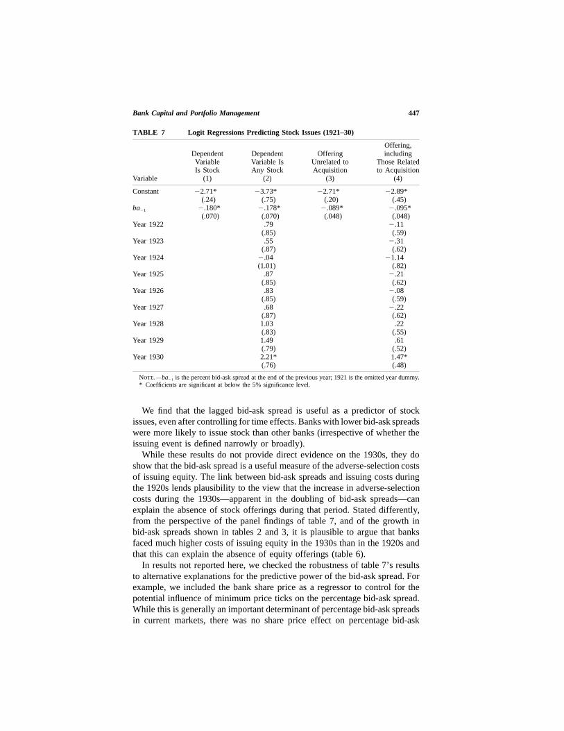
Table 6 presents data on the timing of stock issues for our sample of banks.Table 7 reports logit results predicting the decision to issue stock. We definethe event of a stock issue in two ways: narrowly (issuing stock unrelated toan acquisition of another bank) and broadly (including stock swaps associatedwith bank acquisitions). We include the lagged bid-ask spread and year in-dicators in our logit regressions for the period 1921–30. The paucity of stockissues after 1930 makes it impossible to extend our logit sample period beyond1930.


TABLE 7 Logit Regressions Predicting Stock Issues (1921–30)

DependentVariableIs Stock

DependentVariable IsAny Stock

OfferingUnrelated toAcquisition

Offering,including

Those Relatedto Acquisition

Variable (1) (2) (3) (4)

Constant �2.71* �3.73* �2.71* �2.89*(.24) (.75) (.20) (.45)

ba�1 �.180* �.178* �.089* �.095*(.070) (.070) (.048) (.048)

Year 1922 .79 �.11(.85) (.59)

Year 1923 .55 �.31(.87) (.62)

Year 1924 �.04 �1.14(1.01) (.82)

Year 1925 .87 �.21(.85) (.62)

Year 1926 .83 �.08(.85) (.59)

Year 1927 .68 �.22(.87) (.62)

Year 1928 1.03 .22(.83) (.55)

Year 1929 1.49 .61(.79) (.52)

Year 1930 2.21* 1.47*(.76) (.48)

Note.—ba�1 is the percent bid-ask spread at the end of the previous year; 1921 is the omitted year dummy.* Coefficients are significant at below the 5% significance level.

We find that the lagged bid-ask spread is useful as a predictor of stockissues, even after controlling for time effects. Banks with lower bid-ask spreadswere more likely to issue stock than other banks (irrespective of whether theissuing event is defined narrowly or broadly).

While these results do not provide direct evidence on the 1930s, they doshow that the bid-ask spread is a useful measure of the adverse-selection costsof issuing equity. The link between bid-ask spreads and issuing costs duringthe 1920s lends plausibility to the view that the increase in adverse-selectioncosts during the 1930s—apparent in the doubling of bid-ask spreads—canexplain the absence of stock offerings during that period. Stated differently,from the perspective of the panel findings of table 7, and of the growth inbid-ask spreads shown in tables 2 and 3, it is plausible to argue that banksfaced much higher costs of issuing equity in the 1930s than in the 1920s andthat this can explain the absence of equity offerings (table 6).

In results not reported here, we checked the robustness of table 7’s resultsto alternative explanations for the predictive power of the bid-ask spread. Forexample, we included the bank share price as a regressor to control for thepotential influence of minimum price ticks on the percentage bid-ask spread.While this is generally an important determinant of percentage bid-ask spreadsin current markets, there was no share price effect on percentage bid-ask


spreads in our sample, partly owing to the fact that the price per share tendedto be high during our period.

The bid-ask spread is not only negatively associated with the decision ofwhether to issue stock, it is also negatively associated with the capital ratiochosen by the bank (E/A), as predicted by our model. Table 8 reports reduced-form regression results for the bank capital ratio. Consistent with our viewthat bid-ask spreads capture adverse-selection costs that discourage a high-risk–high-equity strategy, we find that the bid-ask spread is negatively as-sociated with the capital ratio chosen by the bank.

While the percentage bid-ask spread is negatively associated with the pro-pensity to raise capital by offering shares on the market (and the averagecapital ratio of banks during our period), our proxy for adverse-selection costsis positively associated with the tendency to accumulate capital internallyduring the 1930s—which was accomplished by cutting dividends. Informationand agency costs encourage the payment of dividends, and cutting dividendsis costly (Miller and Rock 1985; Ofer and Siegel 1987). Indeed, the fact thatNew York banks were paying dividends while simultaneously raising signif-icant amounts of equity during the 1920s provides prima facie evidence thatpaying dividends was valuable to our sample firms.

Table 9 reports dividend data retrospectively for 1929 and 1939, for thebanks included in our 1939 sample. Dividend reduction was often large duringthe 1930s, and there is substantial cross-sectional variation in the extent towhich banks cut dividends.

In table 10, we report panel OLS results for the annual percentage growthof nominal dividends for banks over the period 1929–39 (the period that sawsignificant reductions in bank dividends). We include the percentage bid-askspread and the default risk on deposits as regressors. Both are significantnegative predictors of dividend growth. Banks experiencing high deposit de-fault risk or a high bid-ask spread were likely to cut dividends more thanother banks. During the adjustment process of the 1930s, the more a bankneeded to reduce its deposit risk (the higher was P), and the harder it wouldbe for the bank to float equity to reduce deposit risk in the future if it had to(the higher was the bid-ask spread, ba), the more the bank reduced currentdividends. Cutting dividends, in other words, was both a way to restore lowdefault risk and to self-insure against the possibility of having to raise (ex-pensive) equity in the future, and the value of that self-insurance was highestfor banks that faced the highest costs of accessing equity in the market.

V. Implications for Arguments about Depression-Era Changes inBank Risk Preferences

One of the lessons of our study is that when examining bank portfolio orfinancing changes during the Depression, it is important to look at both sidesof the balance sheet at the same time. Previous analysis of the behavior ofbanks can be criticized for not having done so. For example, Berger et al.


TABLE 8 Reduced-Form Regressions for Bank Capital Ratio

1920–40 1920–40 1920–28 1920–28 1929–40 1929–40Variable (1) (2) (3) (3�) (4) (4�)

Constant .178* .076* .254* .039* .087* .023(.010) (.018) (.017) (.012) (.020) (.017)

Trust Co. .029* .039* .056* .005 .019 .010(.010) (.008) (.012) (.007) (.012) (.010)

Nat. Bank .009 .016 .021 .004 .009 .008(.010) (.009) (.012) (.007) (.014) (.011)

ba �.005* �.0023* �.0030 .0002 �.0023* �.0023*(.001) (.0009) (.0019) (.0018) (.0010) (.0009)

E/A�1 .0095 .0062*(.0003) (.0004)

Year 1920 .049* �.136* �.043*(.022) (.020) (.011)

Year 1921 .063* �.123* �.023*(.022) (.020) (.011)

Year 1922 .058* �.128* �.035*(.020) (.018) (.011)

Year 1923 .060* �.125* �.029*(.020) (.018) (.010)

Year 1924 .073* �.112* �.027*(.020) (.018) (.010)

Year 1925 .098* �.085* �.009(.019) (.017) (.010)

Year 1926 .102* �.082* �.026*(.020) (.017) (.009)

Year 1927 .159* �.026 .010(.019) (.017) (.009)

Year 1928 .186*(.020)

Year 1929 .180* .181* .066*(.020) (.020) (.019)

Year 1930 .122* .123* .022(.019) (.019) (.018)

Year 1931 .069* .070* �.001(.021) (.021) (.018)

Year 1932 .081* .083* .055*(.023) (.023) (.019)

Year 1933 .036* .038 .007(.023) (.022) (.019)

Year 1934 .028 .030 .022(.023) (.023) (.019)

Year 1935 .051* .053* .051*(.023) (.023) (.019)

Year 1936 .046* .048* .029(.023) (.023) (.019)

Year 1937 .017 .019 .002(.023) (.023) (.019)

Year 1938 .012 .014 .018(.023) (.023) (.019)

Year 1939 .024 .025 .031(.023) (.022) (.018)

Adjusted R2 .052 .318 .266 .851 .332 .595

Note.—The dependent variable is market capital-to-asset ratio (E/A). Standard errors are in parentheses;ba is the contemporaneous percent bid-ask spread for bank stock; Trust Co. and Nat. Bank are indicatorvariables for state trust companies and national banks; 1940 is the omitted year dummy in cols. 2, 4, and 4�;and 1928 is the omitted year dummy in cols. 3 and 3�.



TABLE 9 New York City Bank Dividend Changes, 1929–39

BankDividend 1929

($million)Dividend 1939

($million)

Bankers Trust Company 30.0 2.0Bank of New York & Trust 20.0 14.0Brooklyn Trust Company 30.0 4.0Central Trust Company 3.0 4.0Chase National Bank 10.5 1.4Chemical National Bank 12.0 1.8National City Bank 7.0 4.0Commercial National Bank & Trust .0 8.0Continental Bank & Trust 8.8 .8Corn Exchange Bank & Trust 12.0 3.0Empire Trust Company 16.0 .6Fifth Avenue Bank 59.0 24.0First National Bank 20.0 15.0Guaranty Trust Company 14.0 7.0Irving Trust Company 7.0 3.6Bank of the Manhattan Company 16.0 .9Manufacturers Trust Company 5.8 2.0New York Trust Company 20.0 4.0Public Bank of New York 4.0 1.5Title Guarantee & Trust Company 36.0 .0United States Trust Company 60.0 60.0

Source.—Moody’s Manual of Investments: Banks, Insurance Companies, Investment Trusts, Real EstateFinance and Credit Companies (New York: Moody’s Investors Service, various years).

Note.—The sample of banks included in this table is restricted to banks in our database (as defined in thedata appendix) that were in existence both in 1929 and in 1939.

(1995, p. 403) conclude that the precipitous decline in bank (book) capital-to-asset ratios after 1933 reflected the effects of government deposit insurance,which relieved banks from having to satisfy depositor discipline.

Friedman and Schwartz (1963), examining the asset side of the banks’balance sheets, arrive at the opposite conclusion. They argue that banks feltobliged to increase their holdings of cash and Treasury securities because ofthe increased risk faced by banks. Friedman and Schwartz argue that thefailure of the Fed to act as a lender of last resort made banks realize that theywere more vulnerable than they had previously thought.

An implication of the Friedman and Schwartz (1963) view is that bankersand depositors would have targeted lower default risk for any given lendingrisk than they did prior to the Depression. Berger et al.’s (1995) view impliesthe opposite—that is, greater tolerance for bank default risk after 1933 thanduring the 1920s.

Our data do not support either implication. The targeted default risk ofdeposits in the late 1930s—like that of the 1920s—was very low. Depositors’tolerance for default risk neither rose (as argued by Berger et al. [1995]) norfell (as implied by our interpretation of the Friedman-Schwartz [1963] view).Once one considers bank capital ratios and asset risk together, New York Citybanks behaved as if they were responding to the same depositor preferencesin the 1920s and the 1930s. Lower capital ratios in the 1930s did not reflectan absence of discipline, and neither did lower asset risk reflect an increase


TABLE 10 Dividend Growth Regressions (1929–39)

Variable (1) (2) (3 )

Constant 3.77 6.75 7.85(4.13) (8.91) (9.21)

ba �1.91* �1.78* �1.81*(.65) (.67) (.75)

P �.115* �.131* �.131(.055) (.057) (.061)

ba�1 �.225(.684)

P�1 .02(.08)

Year 1929 11.31 11.42(11.01) (11.15)

Year 1930 �22.31* �22.38*(10.75) (11.00)

Year 1931 �1.16 �1.35(11.12) (11.27)

Year 1932 �9.70 �9.74(11.76) (11.90)

Year 1933 �11.12 �11.16(11.75) (11.87)

Year 1934 �2.12 �2.55(11.81) (12.00)

Year 1935 �2.86 �3.09(11.81) (11.91)

Year 1936 �.74 �.65(11.69) (11.81)

Year 1937 1.89 2.27(11.66) (11.83)

Year 1938 .36 .26(11.66) (11.76)

Adjusted R2 .05 .06 .05

Note.—The dependent variable is annual percentage change in dividends. Standard errors are in parentheses;ba and P are the end-of-year percent bid-ask spread and deposit default premium; and 1939 is the omittedyear dummy.


in risk aversion. Rather, the level of discipline was unchanged, but bankschose to substitute lower asset risk for lost capital because the cost of issuingnew capital had risen. We also note that the fact that New York City banksreduced their capital during the Depression is prima facie evidence againstthe view that deposit insurance caused that decline more generally, since NewYork City banks enjoyed very little benefit from federal deposit insuranceowing to the large deposits held in those banks (Saunders and Wilson 1995).

VI. Conclusion

Recent theoretical work in banking and corporate finance under asymmetricinformation emphasizes that depositors may be intolerant of default risk ontheir deposits and may reward banks for keeping default risk low. Informationproblems also make it more costly for banks to issue stock. Other relatedwork on banking sees bankers as information producers and managers who


earn quasi rents through risky lending, based on possessing scarce information.Our theoretical framework combines these insights (along with standard con-tingent claims pricing) to solve for the equilibrium asset risk choices, andfinancing choices, of banks.

We apply this framework to New York City banks during the period1920–40. Our findings support the key theoretical propositions developed inSections II and III. Capital ratios and asset risk are alternative means thatbanks use to limit deposit default risk. Normally, banks strive to keep defaultrisk low to avoid withdrawals by risk-intolerant depositors. In response to thecapital losses of the Depression, banks substituted into low-risk assets asquickly as possible and cut dividends. Still, they were forced to let their defaultrisk rise temporarily. Over time, as loan liquidation proceeded, default riskreturned to its low long-run equilibrium levels.

Deposit outflows were the inevitable cost of choosing not to liquidate loansfaster or issue new capital. Banks that suffered larger increases in default riskduring the Depression suffered greater percentage shrinkage in their depositbase and made larger cuts to dividends. The reason that banks did not issuenew capital in the 1930s was the higher adverse-selection costs (reflected inwider bid-ask spreads) associated with bank stock in the wake of theDepression.

Our findings indicate no long-run change in the tolerance for deposit riskfollowing the Great Depression. We find that banks in the mid-1930s achievedthe same level of default risk on deposits via a different combination of capitaland asset risk.

Our findings have general implications for the literature on “capitalcrunches,” and for the Fisher (1933) and Bernanke (1983) interpretation ofbank credit reduction during the Depression. We have argued that New YorkCity banks faced binding financing constraints that reduced the supply of bankloans. Loans did not decline solely because of the reduced opportunities forprofitable lending. Banks scrambled to shed asset risk during this period, torestore their default risk to the low long-run desired level, and to avoid thehigh cost of issuing capital as an alternative means to reduce default risk.Avoiding the prohibitive cost of issuing capital entailed a costly adjustmentprocess—banks balanced the costs of forgone lending opportunities, disruptivedeposit withdrawals, and stockholder displeasure at draconian reductions individends.

Despite the support we provide for the Fisher (1933) and Bernanke (1983)view, our analysis also contains a cautionary note. While we have shown thatbank lending was constrained in the early 1930s by the capital losses of theGreat Depression, we have not shown how much higher bank lending wouldhave been in the absence of those constraints. Our model of bank risk andfinancing choices (depicted in fig. 2) illustrates why it is difficult to determinethe precise extent to which a collapse of lending is caused by lost bank capital.A movement from X to Z in figure 2 reflects some combination of a highercost of capital and reduced lending opportunities (lower bank quasi rents from


lending). While we have argued that financing constraints were importantbinding constraints during the 1930s, we cannot address empirically the coun-terfactual question of how much lending would have declined simply due tothe decline in lending opportunities because we lack a good measure of thequasi rents from bank lending.

Finally, our evidence—that (1) markets and depositors discriminate acrossbanks when measuring risk, (2) depositors apply market discipline selectivelyto reward prudence, and (3) the threat of discipline leads banks to reduceasset risk following capital losses—suggests potential gains from reintroducingmarket discipline into banking. Government safety nets can eliminate theincentive to reduce asset risk in the wake of losses. Indeed, protected banksmay increase risk after capital losses (to maximize the value of the safety netsubsidy). Requiring banks to meet market standards for prudence could mit-igate such moral hazard problems and reduce the vulnerability of bankingsystems to collapse (see also Calomiris 1997; and Shadow Financial Regu-latory Committee 2000).

Data Appendix

The data sample comprises an annual bank balance sheet, dividend, and stock issuancedata and weekly stock price data for a sample of New York City banks whose bidand ask quotes were reported in the Commercial and Financial Chronicle and whosestock was actively traded over the period 1920–39. In 1920 (1939), this sample includedapproximately 55 (32) banks, with the largest decline in sample bank numbers duringthe early 1930s. The sample consists of national banks, state banks, and trust com-panies, ranging in size from large-money-center banks to smaller borough and suburbanbanks.

Annual bank-specific balance sheet data, including capital, surplus, deposits, cash,securities, loans, and total assets, were collected from Rand McNally Bankers Direc-tory. The balance sheet data were also cross-checked for accuracy with Moody’sManual of Investments, which began publication in 1928. This latter resource alsoallowed us to collect detailed historical accounts of bank capital levels, new capitalissues, dividends, and stock dividends and splits.

Bid-ask spreads, market values of capital, and equity returns volatility were cal-culated from stock prices reported weekly in the Commercial and Financial Chronicle.Specifically, the average of reported bid and ask quotes was used to develop a weeklystock series for each bank, which was then adjusted for stock splits and stock dividends.The standard deviation of equity returns was then calculated, based on the 6 monthsof weekly stock prices preceding the report date, for the bank’s (year-end) balancesheet data. The Black and Scholes (1973) model, and a double-liability variant of thatmodel used for the period through 1933, were used to derive implied asset volatilitysA (the standard deviation of asset returns) and deposit default premiums from ourmeasures of market capital values, book values of debt, and equity returns volatility.


References

Altmkilic, Oya, and Robert S. Hansen. 1997. Is the marginal cost of external finance rising?Evidence from the direct cost of raising capital in the primary markets. Working paper, VirginiaPolytechnic Institute and State University.

Baer, Herbert L., and John N. McElravey. 1993. Capital shocks and bank growth. EconomicPerspectives 17 (July–August).

Balke, Nathan S., and Robert J. Gordon. 1989. The estimation of prewar gross domestic product:Methodology and new evidence. Journal of Political Economy 97 (February): 38–92.

Barger, Harold. 1942. Outlay and income in the United States, 1921–1938. New York: NationalBureau of Economic Research.

Berger, Allen N., Richard J. Herring, and Giorgio P. Szego. 1995. The role of capital in financialinstitutions. Journal of Banking and Finance 19 (June): 393–430.

Bernanke, Ben S. 1983. Nonmonetary effects of the financial crisis in the propagation of theGreat Depression. American Economic Review 73 (June): 257–76.

Bernanke, Ben S., and Cara S. Lown. 1991. The credit crunch. Brookings Papers on EconomicActivity, 1991, no. 2, pp. 205–48.

Black, Fischer, and Myron Scholes. 1973. The pricing of options and corporate liabilities. Journalof Political Economy 81 (May–June): 637–54.

Board of Governors of the Federal Reserve System. 1976. Banking and monetary statistics,1914–1941. Washington, DC: Board of Governors of the Federal Reserve System.

Calomiris, Charles W. 1993. Financial factors in the Great Depression. Journal of EconomicPerspectives 7 (Spring): 61–85.

———. 1995. The costs of rejecting universal banking: American finance in the German mirror,1870–1914. In The coordination of activity within and between firms, ed. Naomi Lamoreauxand Daniel Raff, pp. 257–315. Chicago: University of Chicago Press.

———. 1997. The postmodern bank safety net: Lessons from developed and developing econ-omies. Washington, DC: American Enterprise Institute.

Calomiris, Charles W., and Charles P. Himmelberg. 2001. Investment banking costs as a measureof the shadow cost of external finance. Working paper, Columbia University.

Calomiris, Charles W., and Charles M. Kahn. 1991. The role of demandable debt in structuringoptimal banking arrangements. American Economic Review 81 (June): 497–513.

Calomiris, Charles W., Charles M. Kahn, and Stefan Krasa. 1992. Optimal contingent bankliquidation under moral hazard. Working paper, University of Illinois at Urbana-Champaign.

Calomiris, Charles W., and Joseph R. Mason. 1997. Contagion and bank failure during the GreatDepression: The June 1932 Chicago banking panic. American Economic Review 87 (De-cember): 863–83.

———. 2003. Fundamentals, panics, and bank distress during the depression. American EconomicReview 93 (December): 1615–47.

Calomiris, Charles W., and Daniel M. G. Raff. 1995. The evolution of market structure, infor-mation, and spreads in American investment banking. In Anglo-American financial systems,ed. Michael D. Bordo and Richard Sylla, pp. 103–60. Homewood, IL: Business One-Irwin.

Campbell, Tim, and William Kracaw. 1980. Information production, market signaling, and thetheory of financial intermediation. Journal of Finance 35 (September): 863–81.

Diamond, Douglas W. 1984. Financial intermediation and delegated monitoring. Review of Eco-nomic Studies 51 (July): 393–414.

Fisher, Irving. 1933. The debt-deflation theory of great depressions. Econometrica 1:337–57.Friedman, Milton, and Anna J. Schwartz. 1963. A monetary history of the United States,

1867–1960. Princeton, NJ: Princeton University Press.Froot, Kenneth A., and Jeremy C. Stein. 1998. Risk management, capital budgeting, and capital

structure policy for financial institutions: An integrated approach. Journal of Financial Eco-nomics 47 (January): 55–82.

Gorton, Gary, and George Pennacchi. 1990. Financial intermediaries and liquidity creation.Journal of Finance 45 (March): 49–72.

Kane, Edward J., and Berry Wilson. 1998. A contracting-theory interpretation of the origins offederal deposit insurance. Journal of Money, Credit and Banking 30 (August): 573–95.

Kashyap, Anil, and Jeremy C. Stein. 1995. The impact of monetary policy on bank balancesheets. Carnegie-Rochester Series on Public Policy 42:151–95.

Leland, Hayne, and David Pyle. 1977. Informational asymmetries, financial structure, and fi-nancial intermediation. Journal of Finance 32:371–87.


Miller, Merton, and Kevin Rock. 1985. Dividend policy under asymmetric information. Journalof Finance 40 (September): 1031–51.

Myers, Stewart C., and Nicholas Majluf. 1984. Corporate finance and investment decisions whenfirms have information that investors do not have. Journal of Financial Economics 5:187–221.

Ofer, Aharon, and Daniel Siegel. 1987. Corporate financial policy, information, and marketexpectation: An empirical investigation of dividends. Journal of Finance 42 (June): 889–911.

Peek, Joe, and Eric S. Rosengren. 1997. The international transmission of financial shocks: Thecase of Japan. American Economic Review 87 (September): 495–505.

Petersen, Mitch, and Raghuram Rajan. 1994. The benefits of lending relationships: Evidencefrom small business data. Journal of Finance 49 (March): 3–37.

Rajan, Raghuram. 1992. Insiders and outsiders: The choice between relationship and arm’s lengthdebt. Journal of Finance 47 (September): 1367–1400.

Ramos, Alberto M. 1995. Bank capital structures and the demand for liquid assets. Workingpaper, University of Chicago.

Romer, Christina. 1989. The prewar business cycle reconsidered: New estimates of gross nationalproduct, 1869–1908. Journal of Political Economy 97 (February): 1–37.

Saunders, Anthony, and Berry Wilson. 1995. If history could be rerun: The provision and pricingof deposit insurance in 1933. Journal of Financial Intermediation 4 (October): 396–413.

Shadow Financial Regulatory Committee. 2000. Reforming bank capital regulation. Washington,DC: American Enterprise Institute.

Slovin, Myron B., Marie E. Sushka, and John A. Polonchek. 1993. The value of bank durability:Borrowers as bank stakeholders. Journal of Finance 48:247–66.

Van den Heuvel, Skander J. 2002. The bank capital channel of monetary policy. Working paper,University of Pennsylvania.

Wilson, Berry, and Edward J. Kane. 1997. The demise of double liability as an optimal contractfor stockholders at large national banks. Working paper, Boston College.

Winton, Andrew. 1993. Limitations of liability and the ownership structure of the firm. Journalof Finance 48:487–512.

Documents

Bank Capital and Portfolio Management: The 1930s … Capital and Portfolio Management 423 our empirical work. Section IV contains the empirical analysis of individual New York City