Electronic copy available at: http://ssrn.com/abstract=1763351

Bank Credit And Business Networks Faculty Research Working Paper Series

Asim Ijaz Khwaja Harvard Kennedy School and NBER

Atif Mian

U.C. Berkeley and NBER

Abid Qamar State Bank of Pakistan (SBP)

March 2011 RWP11-017

The views expressed in the HKS Faculty Research Working Paper Series are those of the author(s) and do not necessarily reflect those of the John F. Kennedy School of Government or of Harvard University. Faculty Research Working Papers have not undergone formal review and approval. Such papers are included in this series to elicit feedback and to encourage debate on important public policy challenges. Copyright belongs to the author(s). Papers may be downloaded for personal use only.

www.hks.harvard.edu

Electronic copy available at: http://ssrn.com/abstract=1763351Electronic copy available at: http://ssrn.com/abstract=1763351

Bank Credit And Business Networks

ASIM IJAZ KHWAJA, ATIF MIAN and ABID QAMAR�

Feb 2011

Abstract

We construct the topology of business networks across the population of �rms in an emergingeconomy, Pakistan, and estimate the value that membership in large yet di¤use networks brings interms of access to bank credit and improving �nancial viability. We link two �rms if they have acommon director. The resulting topology includes a �giant network� that is order of magnitudeslarger than the second largest network. While it displays �small world�properties and comprises5 percent of all �rms, it accesses two-thirds of all bank credit. We estimate the value of joining thisgiant network by exploiting �incidental�entry and exit of �rms over time. Membership increasestotal external �nancing by 16.6 percent, reduces the propensity to enter �nancial distress by 9.5percent, and better insures �rms against industry and location shocks. Firms that join improve�nancial access by borrowing more from new lenders, particularly those already lending to their(new) giant-network neighbors. Network bene�ts also depend critically on where a �rm connectsto in the network and on the �rm�s pre-existing strength.

Keywords: Business Networks, Financial Development, Network AnalysisJEL: L14, O16, D85, D02

�Harvard University, Kennedy School of Government and NBER; U.C. Berkeley and NBER; and State Bank ofPakistan (SBP) respectively. E-mails: akhwaja@ksg.harvard.edu, atif@haas.berkeley.edu and abid.qamar@sbp.gov.pk.We thank seminar participants at Harvard University, Hitotsubashi University, the World Bank, and NBER CorporateFinance and Entrepreneurship Meetings for helpful comments and suggestions. The superb research assistance of NathanBlecharc, Alexandra Cirone, Benjamin Feigenberg, Magali Junowicz, and Sean Lewis-Faupel is greatly appreciated.Special thanks to the Central Bank of Pakistan for answering numerous questions and for help in assembling the dataset. However, the results in this paper do not in any way necessarily represent those of the Central Bank of Pakistan.All errors are our own.

1

Electronic copy available at: http://ssrn.com/abstract=1763351

We live in a remarkably networked global economy. Whether through social relations or business

ties, network links are thought to generate signi�cant value. Several papers emphasize the importance

of networks as conduits of information and enforcement, with networks adding value by facilitating

the transaction of services, such as �nancial intermediation or employment/customer access, that rely

on the quality of information and contract enforcement1. While their role and value may change as

markets develop, networks remain salient even in developed nations.

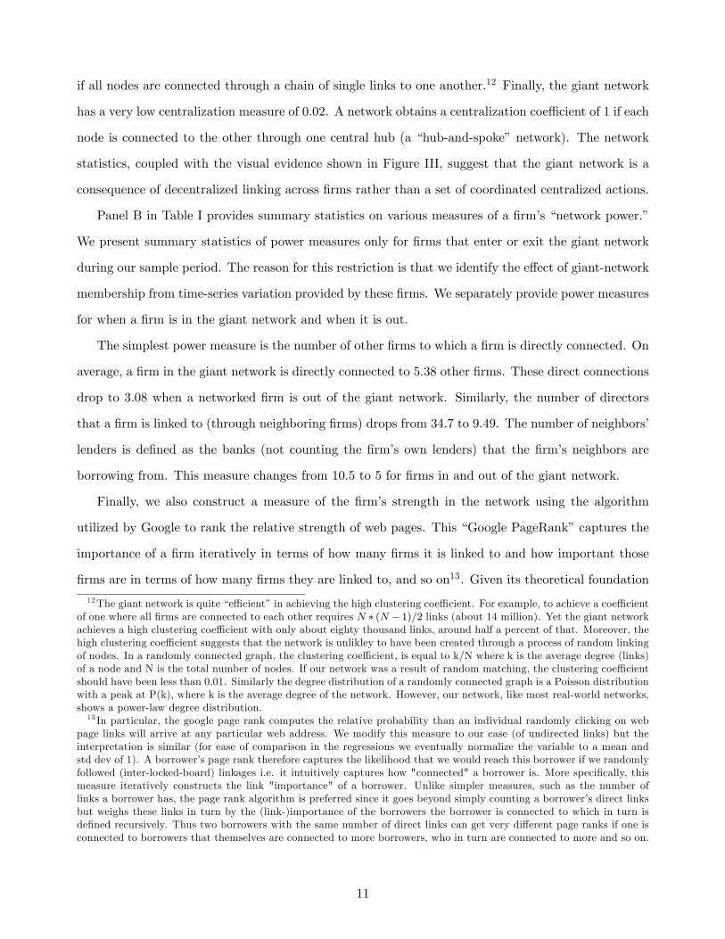
Figure I graphs the network topology in the population of large/public �rms in two developed (the

United States and the United Kingdom) and two emerging (India and Pakistan) economies. Firms are

linked if they have a director in common and drawing connections iteratively allows one to construct

a network topology. Despite large institutional and economic di¤erences, not only do networks appear

equally salient across countries but the network structure appears strikingly similar.2 In particular,

each country has one large network (henceforth referred to as the �giant network�) which is orders of

magnitude larger than the next largest network.

The existence of such a large network is in fact a common occurrence both in network theory (re-

ferred to as the �giant component/cluster�) and in a large literature that examines real-world networks

(see Albert and Barabasi 2002 for a review).3 The giant networks in Figure I have a di¤use and robust

structure that displays �small world� properties (small distance between nodes with relatively high

local inter-connectedness), have a low degree of �centralization� and encompass around half of the

sample �rms. Moreover, the network characteristics suggest that such giant networks are the result of

a decentralized process of local link formations rather than the outcome of any central coordination.

This paper estimates the value in terms of bank credit that a �rm obtains by joining such a business

1For example, Banerjee and Munshi, 2004; Fisman and Khanna, 2004; Le¤ 1976, 1979; McMillan and Woodru¤, 1999;Mobius and Szeidl, 2007; Uzzi, 1999; and Cohen et al 2008.

2These countries were picked based on data availability. We used three di¤erent data sources - Boardex, OneSourceand Pakistan�s central bank. The former two sources typially provide information only on publicly listed and/or largerunlisted companies. The US and UK had more readily available/comprehensive data (Canada, the next most listedcountry in the Boardex database after the U.K., had less than a �fth as many �rms listed), and we choose India forregional comparison with Pakistan. We should note that the seemingly �denser�apperance of the giant networks in theUS and India in Figure I is a function of the larger �rm sample size for those countries and that all four giant networksshow similar network characteristics. We restrict the main analysis in this paper to just one emerging country (Pakistan)since we were able to obtain a much more comprehenesive �rm database which includes both �rm directors/ownersand �rm �nancial access for all �rms borrowing from any formal lending institution in the economy. This allows us totake better advantage of our empirical methodology of focusing on changes in network membership and �incidental�entry/exit.

3Erdos and Renvi (1959 and 1960) show that even random matching of nodes in a system is likely to produce a giantcluster. However, most real networks - including the ones shown in Figure I �are unlikely to have been generated by arandom matching process since they display a much higher clustering coe¢ cient (a measure of inter-connectedness) thana randomly-connected graph would and the degree (number of links) distribution of the nodes follows a power law ratherthan a Poisson distribution that one would expect under random matching.

2

giant network. Our focus on the giant network has two main advantages. First, as pointed above, the

giant network structure is common acrosss the world. Second, as explained below, we provide a new

methodology based on �incidental entrants�to estimate a plausibly unbiased estimate of the impact

of network membership. Such a methodology requires the entry and exit of small networks of �rms

into a larger network.

There are a variety of empirical challenges in trying to estimate the impact of business networks

on �rm outcomes. First, one needs data on the entire population of agents in the economy in order to

construct an accurate topology of connections. In the case of business networks, most data sets that

provide board/owner information cover only publicly listed or large companies. Since smaller private

�rms form the overwhelming majority of business enterprises, any network analysis limited to large or

public �rms may miss important links. Second, networks are the cumulative result of strategic choices

that agents make when forming relationships. Therefore, one must be careful in separating the causal

e¤ect of networks from possibly spurious selection e¤ects (i.e., business networks may select �rms to

join based on unobserved �rm characteristics which a¤ect future �rm performance). Finally, network

theory highlights that network bene�ts depend critically on where in the network one is connected.

One therefore needs to be able to examine such heterogeneity by utilizing credible measures of network

strength, such as the �linkage power� of a node, in order to better understand the process through

which networks bring value.

We address these challenges using novel �rm level data that covers the universe of more than 100,000

�rms in Pakistan over a four year period and by exploiting a methodology that can be replicated in

other settings, for both other economies and other sectors or outcomes. The data comes from the

central bank of Pakistan, which supervises the banking sector, and contains information on each

�rm�s lending relationships, credit history, and importantly, identifying information for the members

of its board of directors. We construct interlocked, board-�rm networks as in Figure I (but for a more

comprehensive sample of �rms) and measure the strength of network connections and nodes using

concepts from graph theory. The giant-network structure remains similar to that in Figure I (see

Appendix Figure I). Importantly, we can accurately track how this network topology changes over

time. This allows us to estimate the value that entry into or exit from the giant network brings in

terms of credit access and �nancial viability. We follow changes in network membership at six-monthly

intervals and look for di¤erences in credit access for �rms that enter or exit the giant network. Our

3

focus on time-series variation in network membership for a given �rm absorbs any unobserved time-

invariant �rm attribute that jointly determines network membership and access to credit.

However, a remaining concern is that entry and exit from the giant network may be driven by time-

varying changes in �rm quality. For example, �rms with better anticipated growth prospects may be

more likely to join the network. If that were the case, an increase in access to credit after entering

the network may be driven by unobserved improvements in �rm quality and not direct bene�ts of the

network, per se.

We address this issue by introducing a methodology for estimating network bene�ts particularly

suited for cases where there is a clearly de�ned giant network. The idea is to focus on the e¤ect of

(giant-)network membership for incidental entrants/exitors and to compare this with the e¤ect for

direct entrants/exitors. Incidental entrants are �rms that enter the giant network not because of any

changes in their board of directors, but because of changes in the board of directors of a neighboring

�rm that they were already linked to. For example, consider Firms A and B with three directors

each and only one director, Director 1, in common. Both �rms are initially not in the giant network.

Now suppose that Firm A enters the giant network because one of its existing directors (other than

Director 1) is invited to be on the board of a giant-network �rm. Firm A has entered �directly�into

the network. Firm B, however, enters the network �incidentally.�It joins the network not because one

of its directors was selected to join a giant-network �rm but only because it happened to be connected

to a �rm (A) that joined the network. Incidental exitors are de�ned analogously.

To the extent that incidental entry/exit occurs due to factors that are unrelated to a �rm�s (future)

performance, the impact on incidentals provides the equivalent of an unbiased instrumental variable

estimate of the impact of network membership. However, one could still argue that focusing on inci-

dentals may not eliminate the time varying selection concern. While it is typically hard to empirically

defend an instrument, an additional advantage of our methodology is that a comparison of the e¤ect

between direct entrants/exitors and incidentals (after matching on �rm attributes) provides an esti-

mate of the sign and severity of the selection e¤ect. Thus, if one �nds, as in our case, that the e¤ect of

network entry/exit is similar for both direct and incidental entrants/exitors, this provides additional

evidence that the time-varying selection is not a serious concern. In other words, on the margin (i.e.

for �rms that enter or exit the giant network during our sample period) even direct entry/exit seems to

be driven by time-varying social factors and not by time-varying �rm performance factors that a¤ect

4

future �rm performance.

We �nd that the impact of giant-network membership is large. It leads to a 16.6 percent increase in

bank credit and a 9.5 percent decline in the propensity to enter �nancial distress. The increase in bank

credit is due to both an increase in average borrowing and the formation of new banking relationships.

New banking relationships re�ect the importance of the �referral channel�: They are more likely to be

formed with banks that already have a lending relationship with one of the immediate giant-network

neighbors of the newly networked �rm.

The bene�ts of giant -etwork membership also depend on where in the network one is connected.

In terms of access to bank credit, �rms bene�t more from entry when they connect to more powerful

parts of the giant network. However, gains in credit access are tempered if a �rm was already powerful

(that is, for bank credit, entry into the giant network is a substitute for a �rm�s pre-existing power

and has diminishing returns). We measure power of a connecting node in a number of di¤erent ways,

including number of direct links to other �rms/directors within the network, the strength of these

neighbor �rms, and a measure analogous to �Google PageRank.�

Overall, our results shed useful light on the likely channels through which network memberships

gives acces to credit. In particular, they favor theories where network bene�ts depend on credible

maintenance of links, rather than theories where network membership acts as a signalling device. We

discuss this in more detail in conclusion.

The role of business networks in improving �rm performance and access to bank credit has been

emphasized in the context of early American history by scholars such as Lamoreaux, 1986. While

there has been considerable work in network theory (see Jackson, 2004), empirical work lags behind.4

Our paper provides three key contributions in this regard. First, it uses the entire population of �rms

in an economy, rather than any speci�c subset, to construct networks. We can thus be reasonably

con�dent that we are not missing important network connections in our analysis.

Second, earlier work mostly focuses on estimating cross-sectional di¤erences between networked

and non-networked �rms, making it di¢ cult to control for unobserved, �rm-speci�c attributes that

determine both network membership and the outcome of interest. Our paper not only uses time-

4Some notable exceptions include: Grief (1993), who examines the role that networks of traders played in overcomingbarriers to international trade; Feenstra et al. (1999), who �nd that networks matter for explaining di¤erences in qualityand variety of exports across South Korea, Taiwan, and Japan; Hoshi, Kashyap, and Scharfstein (1991), who show theimportance of networked �rms in getting access to credit in Japan; Hochberg et al. (2007), who show that better-networked VC funds are correlated with better performance; and Khanna (2000), who in a series of papers also examinesthe structure and importance of business groups.

5

series changes in network membership for a given �rm, thus enabling the use of �rm �xed e¤ects to

address unobserved, �rm-speci�c factors that may in�uence network membership, but can also address

additional concerns of time-varying �rm-level unobservables. It does so both through non parametric

controls and the use of incidental entrants as potential instruments and a means of identifying any

(remaining) selection e¤ects.

A third contribution of our paper is that we do not treat the network as a homogenous entity.

As frequently noted by sociologists (e.g., Burt 1992, Granovetter 1973) and economic theorists (e.g.,

Jackson and Wolinsky, 1996; Johnson and Gilles, 2000; Belle�amme and Bloch, 2002; Calvo-Armengol

and Jackson, 2001; Kranton and Minehart, 2001), not all nodes and links within a network are created

equal. Hence, the value of a network to its members is not uniformly distributed but depends on where

and with whom a �rm is connected. Moreover, �rms of di¤erent initial power may bene�t di¤erentially

from the network. While previous studies have rarely examined such heterogeneity of network e¤ects,5

we are able to make headway due to our ability to observe both pre- and post-entry variation in �rm

power attributes.

I De�ning Business Networks

A. Data & Context

We use two data sets in this paper, both from the central bank of Pakistan. The �rst data

has information on the board of directors of all borrowing �rms in the economy from 1999 to 2003

at six-month intervals. The second has detailed loan level information on these �rms� borrowing

over the same period at a quarterly frequency. We describe each of these below. However, before

doing so, we should note that both the industrial and banking sector in Pakistan is fairly liberal and

representative of emerging markets. There are few restrictions on �rm entry and exit and while there

are large state companies in several sectors, there is substantial foreign/multinational and domestic

private sector presence. While �rms do face a variety of market obstacles and ine¢ ciencies, these are

not signi�cantly di¤erent from those in other emerging economies. Private, foreign, and government

banks constitute roughly equal shares of domestic lending. Financial reforms in the early 1990s

brought uniform prudential regulations in-line with international banking practices (Basel Accord),

5A recent review article by Rauch and Hamilton (2001) makes the same point.

6

and autonomy was granted to the central bank for regulation. While some political e¤orts have

been made to bring banking in accordance with Islamic shariah laws, it has not had any signi�cant

functional impact on banking. For all practical purposes, banking follows global norms with deposit

and lending rates determined by the market. While we are not comfortable going so far as to claim

our results (on the value generated by network membership) readily generalize to other settings, it is

nevertheless reassuring that Pakistan�s industrial/banking sector and �rm network topology does not

appear atypical of emerging economies.

(i) Board of Directors Information

The central bank of Pakistan maintains a list of the board of directors of all �rms borrowing from

any bank in the country. We have this data from 1999 to 2003 at a semiannual frequency for well over

100,000 �rms that represent the universe of all borrowing �rms in the economy. The data records the

full name, father�s name, national identi�cation card (NIC) number, and percentage of equity held for

each director of a �rm at a given point in time.

Since we ultimately want to link two �rms together if they have a director in common, it is

important to uniquely identify individuals in our board of directors data set. The NIC number issued

by the government serves this purpose, as it is unique to every individual. However, reporting of the

NIC number is not mandatory, and this information is missing or incomplete around 16 percent of the

time. When we do not have NIC information, we identify and track individuals over time and across

�rms by matching an individual�s full name and their father�s full name (or husband in the case of

married women). We deliberately utilize a stringent criteria for matching director names so as not to

incorrectly connect two �rms. Our matching criteria gives us a total of 261,069 unique directors for

139,526 �rms in our sample. In our �nal sample, we drop very small �rms with less than Rs.500,000

(about US $8,500) of borrowing at the beginning of our sample period since these �rms have very

noisy loan amounts, frequently going from positive to zero amounts. Exclusion of these �rms leaves

us with a total sample of 105,917 �rms. The results are qualitatively similar even if these �rms are

included.

7

(ii) Firm Borrowing Information

We also have quarterly information on a �rm�s loan from any bank it borrows from over a seven-

year period from 1996 to 2003. The data is at the level of a loan (i.e., �rm-bank pair) and traces

the history of �rm borrowing with information on the amount of the loan (principal and interest),

outstanding balance, and amount in default. The outstanding loan amount is further broken down

into di¤erent categories, such as term loans, working capital, etc. The default amount starts appearing

in our data set as soon as a loan payment is overdue by thirty days or more. Although the original

data is at the level of the loan, for most of our analysis, we aggregate loans to a given �rm across its

lenders at a given point in time. Since the director data is available at six month frequencies from

1999 to 2003, we only use the loan data that corresponds to these time periods.6

In terms of data quality, our personal examination of the collection and compilation procedures, as

well as consistency checks on the data, suggest that it is of very good quality. Our data was part of an

e¤ort by the central bank to set up a reliable information sharing resource that all banks could access.

A credible signal of data quality is that all banks refer to this information on a daily basis to verify the

credit history of prospective borrowers. Our checks with one of the largest and most pro�table private

banks in Pakistan revealed that they use the information about prospective borrowers explicitly in

their internal credit scoring models. We also ran several internal consistency tests on the data, such

as aggregation checks, and found it to be of high quality. As a random check, we also showed the data

from a particular branch of a bank to that branch�s loan o¢ cer who con�rmed the authenticity of the

data related to his portfolio.

B. Network Description

We use information on �rm directors to construct networks and link two �rms if they share a

common director (i.e., have interlocked boards).7 Figure II illustrates the hypothetical construction

of a network through this process. There are eight �rms in the example (A through H), and a total of

�fteen directors sitting on the board of these �rms (numbered 1 through 15).

Interlocked board linkages produce two distinct networks and two �rms (G and H) that are not

connected to anyone else. The largest network consists of Firms A through D, where Firms A, B,

6We use 1996-1998 data to construct lagged measures of loan growth and change in default.7Our use of interlocked directorates to de�ne networks has a long tradition among social scientists (e.g., Mintz and

Schwartz, 1985; Stokman et al., 1985; Scott, 1987).

8

and C are linked to each other directly and Firm D is linked to Firms A and B indirectly through its

direct link with C. Thus, �rms in the same network may be linked to each other through long chains

of indirect links.

A second feature to take away from Figure II is that �rms within a network vary by how �impor-

tant� they are in the network. For example, Firm C is important in the network because it has the

most number of �rms directly connected to it (three �rms). Similarly, links between �rms can vary

in their �strength.�For example, Firms E and F are connected to each other through three directors

(the number on the link represents the number of directors generating the link). We shall exploit such

heterogeneity in the strength of network nodes and links to test if the strength of connections is also

important in determining the advantage that networks bring to connecting �rms.

We apply the principle outlined in Figure II to construct networks at a point in time. Doing so

gives us eight snapshots of the structure of business networks in Pakistan - once for every six months

from 1999 till 2003. As a consequence, we can not only observe how networks evolve over time but

also isolate the entry and exit of individual �rms from speci�c networks. Almost two-thirds (66,140)

of �rms are never linked to any other �rm at any point in time. The remaining third of �rms belong to

multi-�rm networks in at least some of the periods (Table I, Panel A).8 The size (that is, the number

of �rms in the network) distribution of multi-�rm networks reveals a striking pattern in every period.

Network size varies in any given period from 2 to 85, followed by a single �giant network�of about

three thousand �rms.9

The size of the giant network, as well as the identity of its �rms, changes over time due to the

addition or removal of directors from �rms or because of �rm creation or dissolution. There are 2,838

�rms that are always part of the giant network and 2,457 �rms that belong to the giant network for

some, but not all, of the periods. Table I, Panel A shows the distribution of �rms by network size

and some summary statistics. While about 5 percent of �rms (5,295) belong to the giant network at

some point in time, the share of these �rms in total bank credit is 65 percent, signifying the relative

economic importance of the giant network. Out of the remaining �rms, precisely 34,482 belong to

networks of size 2 through 85 at some point during our sample period. These �rms collectively borrow

about 21 percent of total bank credit, with the remaining 15 percent going to non-networked �rms.

8See Appendix Figure 1 for all the network structures in the economy.9The giant-network size varies somewhat in each time period but remains within two and a half to three thousand

�rms. This results in over �ve thousand distinct �rms that are in the giant network at some point in the four-year period.

9

Figure III (Panel A) illustrates the giant network by taking a union of the giant networks over

the eight six-month periods. Firms that always remain inside the giant network are represented by

black dots, while �rms that enter and/or exit the giant network are represented by red dots. Firms

are linked if they share a common director at some point in time. The large number of �rms and high

density of links in the giant network make it di¢ cult to see the intra-network details in the top-panel

of Figure III. We therefore zoom into a couple of di¤erent areas of the giant network to provide more

clarity as to what the network structure looks like. Panel B zooms into an area closer to the �core�

of the giant network.10 While each dot represents a �rm, the number inside the dot represents the

number of �rms that the �rm is connected to. Panel C zooms in to a more peripheral area of the giant

network where �rms have a lot fewer connections to other �rms.

Figure III highlights a couple of important giant network characteristics. First, the network is

quite strongly interconnected, with no single �hub� �rm (or a small subset of such �rms) holding

the entire network together. The number of links per �rm is relatively small even in the core of the

giant network (Panel B). Moreover, robustness tests shows that even after the removal of �rms that

have the most number of links, the giant network retains its overall structure (see the appendix for

more details on this and other related checks regarding the robustness of giant-network structure). A

second feature re�ected in the �gures is that there is heterogeneity in the strength with which a �rm is

connected to the giant network. Some �rms hang on to the giant network with one or two connections,

while others are very strongly interconnected with multiple links. Similarly, some �rms are connected

to more �powerful��rms within the giant network than others.

A number of network statistics suggest that our giant network displays �small-world�properties

(Jackson and B. Rogers, 2005; Watts and Strogatz, 1998). The average distance (number of links)

between any two �rms is 6.5 links, surprisingly close to the canonical �six degrees of separation�

example. The maximum distance (diameter) between any two �rms in the network is twenty-three,

which is quite low given the total size of the network.11 The network displays a reasonably high degree

of clustering, with a clustering coe¢ cient of 0.65. A maximum clustering coe¢ cient of one re�ects that

each node is fully connected to every two nodes around it. A network has a clustering coe¢ cient of zero

10The graphs were plotted using Cytoscape. The software computes the �centrality� of every node before decidingwhether to place a node in the center or at the periphery. For example, an important node with many connections toother �rms within the network is likely to be placed closer to the core of the network structure. On the other hand, anode with a few connections is more likely to sit at the periphery of the network structure.11For example, in a linear network, the diameter would have been one less than the total number of �rms in the

network (over �ve thousand in our case).

10

if all nodes are connected through a chain of single links to one another.12 Finally, the giant network

has a very low centralization measure of 0.02. A network obtains a centralization coe¢ cient of 1 if each

node is connected to the other through one central hub (a �hub-and-spoke�network). The network

statistics, coupled with the visual evidence shown in Figure III, suggest that the giant network is a

consequence of decentralized linking across �rms rather than a set of coordinated centralized actions.

Panel B in Table I provides summary statistics on various measures of a �rm�s �network power.�

We present summary statistics of power measures only for �rms that enter or exit the giant network

during our sample period. The reason for this restriction is that we identify the e¤ect of giant-network

membership from time-series variation provided by these �rms. We separately provide power measures

for when a �rm is in the giant network and when it is out.

The simplest power measure is the number of other �rms to which a �rm is directly connected. On

average, a �rm in the giant network is directly connected to 5.38 other �rms. These direct connections

drop to 3.08 when a networked �rm is out of the giant network. Similarly, the number of directors

that a �rm is linked to (through neighboring �rms) drops from 34.7 to 9.49. The number of neighbors�

lenders is de�ned as the banks (not counting the �rm�s own lenders) that the �rm�s neighbors are

borrowing from. This measure changes from 10.5 to 5 for �rms in and out of the giant network.

Finally, we also construct a measure of the �rm�s strength in the network using the algorithm

utilized by Google to rank the relative strength of web pages. This �Google PageRank�captures the

importance of a �rm iteratively in terms of how many �rms it is linked to and how important those

�rms are in terms of how many �rms they are linked to, and so on13. Given its theoretical foundation

12The giant network is quite �e¢ cient�in achieving the high clustering coe¢ cient. For example, to achieve a coe¢ cientof one where all �rms are connected to each other requires N � (N � 1)=2 links (about 14 million). Yet the giant networkachieves a high clustering coe¢ cient with only about eighty thousand links, around half a percent of that. Moreover, thehigh clustering coe¢ cient suggests that the network is unlikley to have been created through a process of random linkingof nodes. In a randomly connected graph, the clustering coe¢ cient, is equal to k/N where k is the average degree (links)of a node and N is the total number of nodes. If our network was a result of random matching, the clustering coe¢ cientshould have been less than 0.01. Similarly the degree distribution of a randomly connected graph is a Poisson distributionwith a peak at P(k), where k is the average degree of the network. However, our network, like most real-world networks,shows a power-law degree distribution.13 In particular, the google page rank computes the relative probability than an individual randomly clicking on web

page links will arrive at any particular web address. We modify this measure to our case (of undirected links) but theinterpretation is similar (for ease of comparison in the regressions we eventually normalize the variable to a mean andstd dev of 1). A borrower�s page rank therefore captures the likelihood that we would reach this borrower if we randomlyfollowed (inter-locked-board) linkages i.e. it intuitively captures how "connected" a borrower is. More speci�cally, thismeasure iteratively constructs the link "importance" of a borrower. Unlike simpler measures, such as the number oflinks a borrower has, the page rank algorithm is preferred since it goes beyond simply counting a borrower�s direct linksbut weighs these links in turn by the (link-)importance of the borrowers the borrower is connected to which in turn isde�ned recursively. Thus two borrowers with the same number of direct links can get very di¤erent page ranks if one isconnected to borrowers that themselves are connected to more borrowers, who in turn are connected to more and so on.

11

and practical success, Google PageRank is our preferred summary statistic for measuring network

power.

II Empirical Methodology

A. Basic Setup

The dominance of the giant network vis-à-vis other smaller networks is illustrated in Appendix

Figure I, which graphically displays the network structures for all borrowing �rms in the economy.

Moreover, as already emphasized in the introduction, both theoretically and empirically, the presence of

giant networks seems to be a common phenomenon. Given the signi�cant, selection-related challenges

in identifying the value of network membership, we develop a methodology that uses giant networks to

do so. While we apply this to business networks in Pakistan and to a speci�c set of outcomes (�nancial

access), the methodology can readily be extended to networks in other sectors and economies, provided

one has comprehensive data that permit an examination of the evolution of these structures over time

and that relate to outcomes of interest.

The challenge in identifying the causal e¤ect of entry into the giant network is that �rms that enter

the giant network might be systematically di¤erent from �rms that do not. Thus, any observed di¤er-

ence between networked and non-networked �rms may be spuriously driven by unobserved �selection�

factors rather than by the direct e¤ect of network membership.

Consider a giant network with n nodes, where each node represents a �rm. Two nodes are linked

if they have a director in common, and all nodes in the network are ultimately connected to each

other through such links. We denote individual nodes with Nm where m varies from 1 to n: There is

a burgeoning literature on how networks form, survive, and evolve over time (see Jackson, 2004, for a

review). However, a full model of network formation is beyond the scope of our paper. We therefore

take the n� node network as given and estimate the impact of network membership on the marginal

�rm joining the network.

Suppose �rm i attempts to join the network every period t by trying to establish a link with an

existing network node. Such a link can be established if one of the board members of �rm i joins

the board of a networked �rm. Alternatively the link can be established if a director of an already

networked �rm joins �rm i�s board.

12

In order to estimate the direct bene�ts of network membership, a key question is: What determines

which �rm i enters the network, and when? Network entry is determined by a selection equation that

speci�es whether and when a �rm enters the giant network. Let hit denote the hazard rate that

�rm i enters the network at time t; conditional on not having entered already. Without much loss of

generality, we assume that hit depends on expected �rm productivity, �it; and �incidental factors,�

xit; that are orthogonal to �rm productivity. An example of incidental factors is social ties that do not

in�uence �rm performance but help a �rm gain entry. It is plausible that �rms with higher expected

productivity and �better�incidental factors are more likely to enter the network:

hit = �(�it; xit; �it) (1)

where � is a cumulative distribution function and �it is an i.i.d random component. For simplicity,

we assume separability of these factors.

�it evolves through a stochastic process such that each �rm starts with a �rm speci�c productivity

�i0 in period 0; and then evolves according to �it = �i;t�1 + �it. �it is a �rm speci�c productivity

shock every period and may not be independent across �rms or over time.

Let Yit re�ect a measure of �rm performance in the credit market that we can use to calculate the

bene�ts of network membership. Our paper uses two such measures: (i) access to external �nance

(which is also closely related to �rm sales and inventory); and (ii) propensity to enter �nancial distress.

In order to illustrate the di¢ culty in identifying the bene�ts of network membership; suppose

we try and do so by comparing the performance of networked and non-networked �rms through the

equation:

Yit = �+ �1ENTRYit + "it (2)

where ENTRYit is an indicator variable for whether �rm i is part of the giant network in period

t: The key concern regarding identi�cation of �1 is that outcomes Yit are likely to depend not only on

network membership, ENTRYit; but also �rm productivity, �it: Since ENTRYit itself is a function of

�it through Equation (1), we have the usual simultaneity/omitted variable problem.

13

B. Identi�cation

We address the possibly spurious e¤ect of �it on b�1 using two types of approaches: non-parametriccontrols and an instrumental variable strategy that uses incidental entry/exit.

14

Non-parametric controls

The �rst approach uses non-parametric controls to absorb �rm speci�c factors that might determine

network entry and �rms� credit market performance simultaneously. A key component of �it that

in�uences entry into the network is the initial productivity level of a �rm, �i0: While we do not

observe this parameter, we can completely absorb it from the estimating equation by including �rm

�xed e¤ects �i in Equation (1). Firm �xed e¤ects account for any level di¤erences in productivity

across �rms.14

However, this still leaves open the concern that �rms are more likely to enter the network at certain

points in time when, for example, the industry they belong to happens to get a series of positive shocks.

We make another non-parametric adjustment to account for such time-varying productivity factors

by including in Equation (2) all interactions of �rm-type �xed e¤ects with time �xed e¤ects (�kt), in

addition to the �rm-�xed e¤ects. Firm type, k; in our regressions includes separate classi�cations for

a �rm�s location, size decile, and industry.

While this addresses a variety of time-varying shocks, �1 may nevertheless be in�uenced by other

time-varying speci�c shocks, �it, that are idiosyncratic to a particular �rm. For example, a given �rm

may be more likely to join the giant network after it receives a series of positive permanent shocks

,f�itg, that are unrelated to its sector, location, or size decile. While we do not observe such �rm-

speci�c shocks, if these shocks were in�uential, conditional on entry in t, a �rm should have a higher

growth trajectory for Y prior to t:

Thus, one can test whether �1 is driven by time-varying shocks to �rm productivity by including

lagged growth rate of Yit and checking if �1 drops substantially. The combination of non-parametric

and lagged growth rate controls gives us the following estimation equation:

Yit = �i + �kt + �t + � 4Yi;t�1 + �1ENTRYit + "it (3)

where �i are �rm �xed e¤ects, �kt is �rm-type (k) interacted with date �xed e¤ects, and 4Yi;t�1 =

Yi;t�1 � Yi;t�2 .15

14Panel A in Table I shows that �rms that are part of the giant network are on average much larger and have much lowerdefault rates than �rms outside the network. Such �xed time-invariant di¤erences between networked and non-networked�rms are absorbed away by the �rm �xed e¤ects.15Since Equation (3) is a �xed e¤ects regression, we need to be careful in including lagged dependent variables.

Including levels of lagged dependent variables would be problematic since the lagged term would be correlated with the�xed e¤ect. While one could correct for this using Arellano-Bond style corrections, our speci�cation uses lagged growthof the dependent variable. Since this lagged term is in changes (i.e. Yi;t�1 � Yi;t�2), the immediate concern that it is

15

Incidental Entry/Exit

Our second approach to addressing potentially endogenous entry into the giant network is based

on exploiting incidental entrants/exitors. We use this both as a potential instrumental variable and

as a way of providing a sense of the biases that may arise from time-varying selection e¤ects.

A limitation of Equation (3) is that, while it is able to address �rm-type time trends and outcome

pre-trends, it is still possible that an unobserved, �rm-speci�c, and time-varying factor in�uences

both network membership and the outcomes of interest. In the terminology of the hazard function

(1), ideally we would like to instrument entry with an incidental parameter xit:

We propose such an instrument based on the �incidental� entry of some �rms into the giant

network. There are two distinct ways in which a �rm can gain entry into the giant network: direct

and incidental. Figure IV, based on our actual data, illustrates the di¤erence between the two.

The example in Panel A shows three �rms before and after they enter the giant network. The

�rms are connected because they each have a director in common, but there is no director common

to all three. Two �rms (#100 and #101, colored as white) join the giant network directly because

their common director is invited to sit on the board of an existing giant-network �rm. The third �rm

(#102), colored in yellow, enters the giant network incidentally as none of its directors are invited to

sit on the board of an existing giant-network �rm.

Panel B depicts another example of incidental and direct entry into the giant network where the

nature of the direct entry is slightly di¤erent. Instead of the direct entrant�s director being invited

to sit on a giant-network �rm�s board, in this case, the direct entrant receives a new director who

also sits on a giant-network �rm�s board. As in the previous example, the three �rms have a common

director and are thus linked to each other. One of the �rms (#106) adds a new director who already

happens to sit on the board of one of the networked �rms. Thus, �rm #106 enters the giant network

directly. Firms #104 and #105 (colored in yellow) join the giant network incidentally since none

of their directors are invited to sit on a giant-network �rm, nor do they add a new (giant-network)

director.16

correlated with the �xed e¤ect is not present as it is di¤erenced out. Moreover, we believe this is a more appropriatecorrection (i.e., we are concerned about controlling for a �rm�s past growth trajectory).16While one could separate incidental entrants based on which of the two types of direct entry their connecting �rm

experiences (Panel A versus Panel B), we do not do so. This is both because of sample size limitations and because thereis no clear reason to think this would improve identi�cation as it is not clear whether one form of direct entry faces astronger selection problem than the other.

16

We analogously de�ne incidental exits; that is, �rms that exit the giant network indirectly because

one of the �rms they are connected to experiences either a removal of a giant-network �rm director

from its board or because one of its directors no longer sits on the board of another giant-network

�rm.

We use incidental entry/exit as an instrument for entry/exit. Incidental entrants/exitors are rea-

sonable candidates for instruments because these �rms join/leave the giant network without any direct

change in the composition of their own board. Similarly, none of their directors takes a seat on the

board of a giant-network �rm. Therefore, incidental �rms are not joining or leaving the giant network

through an active decision that involves their board. As such, it is likely that incidental entry/exit is

orthogonal to changes in �rm level fundamentals and hence to a �rm�s future trajectory.

Furthermore, there is empirical evidence to support this. If incidental entrants enter the giant

network by chance, there should not be any signi�cant di¤erence between incidental entrants prior to

giant-network entry and other similar �rms that (by chance) do not enter the giant network. In order

to test this condition, it is important to understand what kind of �rms have the potential to become

incidental entrants.

A �rm can enter the giant network incidentally only if it is connected to some other �rms, one

of which enters the giant network directly. Thus, standalone, non-networked �rms can never become

incidental entrants. More importantly, the probability of incidental entry likely monotonically increases

with the size of the network that a �rm belongs to before entry into the giant network. Therefore, the

natural comparison cohort of incidental entrants belonging to a network of size k at time t� 1 is the

set of non-entrant �rms at time t� 1 that also belong to a network of size k but never enter the giant

network.

Figure V compares �rms in networks of various sizes. Panel A illustrates sample networks of

various sizes k that end up entering the giant network at some point during our sample period. While

a few of the �rms in each network enter directly, the remaining �rms enter incidentally. Figure V(B)

illustrates a comparison sample of �rms. These �rms also belong to various networks of size k; but

they never enter the giant network. As an example, consider the two networks with k = 6 in Figures

V(A) and V(B), respectively. For the sake of argument, suppose that one of the �rms in V(A) network

enters directly, with the remaining entering incidentally. If incidental entry is truly driven by factors

orthogonal to �rm performance, then the �ve �rms that happen to enter the giant network incidentally

17

in Figure V(A) should be no di¤erent (prior to giant-network entry) than the six in the k = 6 network

in Figure V(B).

We check whether this is true in our data by using pre-entry network-size �xed e¤ects and com-

paring outcomes for incidental �rms, prior to giant-network entry, with their relevant cohort (of

non-entering) �rms. We check for di¤erences on our two key performance metrics, growth in bank

credit and changes in default status. The result shows that there is no di¤erence between incidental

�rms and �rms that do not enter the giant network in either of the two metrics. The di¤erence in

growth rate of bank credit between incidental entrants and non-entrants belonging to same-sized net-

works is less than 0.5 percent and insigni�cant (p-value of 0.84). Similarly, the di¤erence in changes in

default rate is less than 0.04 percent and insigni�cant (p-value of 0.89). These results lend support to

our identi�cation strategy. For example, if incidental entrants were improving prior to giant-network

entry, they should have had relatively declining propensity to default compared to similarly networked

�rms that do not enter. As our results show, this is not the case.

In addition, one can ask whether incidental entrants�and exitors�performance (while they are out

of the giant network) co-varies with that of the �rms whose direct exit or entry caused the incidental

change in giant-network membership. Were this the case and even if only a direct entrant/exitor was

purposely selected to join the giant network, one may be concerned, for instance, that those �rms who

are incidentally joining the giant network would also show an improvement because of an underlying,

pre-existing correlation between incidental and direct giant-network members. As an additional check,

we �nd that, conditional on the �rm attributes which we control for in our speci�cations, there is

no signi�cant correlation in either borrowing size or default rates between direct entrants and their

incidental companions when both are out of the giant network.

Since incidental entrants and exitors are a strict subset of the �rms that enter the giant network,

the IV estimate is analogous to separately estimating the impact on incidental and direct entrants.

We therefore augment the previous speci�cation and estimate:

Yit = �i + �kt + �t + � 4Yi;t�1 + �1ENTRYit + �2ENTRYit �Directi + "it (4)

where Directi indicates a �rm which at some point directly enters/exits the giant network. �1

is our coe¢ cient of interest (the analogous IV estimate) since it isolates the impact of giant-network

membership on the incidental entrants/exitors.

18

Like in all IV estimates, �1in Equation (4) is, therefore, e¤ectively a local average treatment e¤ect

(LATE) and does not estimate the overall average treatment e¤ect (ATE) of entry into the giant

network. Recall that the LATE estimator can di¤er from the average treatment e¤ect if the subset

of �rms a¤ected by the instrument are systematically di¤erent and if there is heterogeneity in the

treatment e¤ect (Imbens and Angrist, 1994). In our framework, �rms a¤ected by the instrument are

the incidental entrants and exitors, and there are plausible reasons to believe that the treatment e¤ect

for these �rms may be di¤erent than the treatment e¤ect for direct entrants.

Incidental entrants enter the giant network indirectly and hence have a �weaker�connection with

the giant network. If the e¤ect of giant-network entry is smaller for �rms that connect weakly, our

LATE estimate will be smaller than the average treatment e¤ect. Fortunately, an advantage of our

data set is that we can directly measure the strength with which �rms are connected to the giant

network, as well as their pre-entry network strength (e.g., the Google PageRank measure explained

earlier). Thus, we can directly test if such heterogeneity in treatment e¤ect is present and control for

it.17

In addition, an advantage of our methodology is that a comparison of the e¤ect between direct

and incidental entrants/exitors (after matching on �rm attributes) provides an estimate of the sign

and severity of the selection e¤ect as long as the potential selection e¤ect is stronger for direct en-

trants/exitors relative to incidental entrants/exitors. In other words, if one �nds, as we do, that the

e¤ect of network entry/exit is similar for both direct and incidental entrants/exitors (once we have

taken treatment heterogeneity into account) this provides additional evidence that the time-varying

selection concern is not serious: that is, even direct entry/exit seems to be driven by time-varying social

factors unrelated to future �nancial borrowing/performance and not by time-varying �rm performance

factors that impact its future �nancial trajectory18.

17Ultimately, our startegy also implies that (even for the direct entrants) we may not be capturing the average treatmente¤ect for the typical �rm in the giant network. Since we identify our e¤ect by utilizing �rm �xed e¤ects, we can onlydo so for �rms that enter/exit the network over time. The estimated e¤ect may be di¤erent from that for a �rm that isso strongly connected that it never exits the giant network. While we are far more cautious in doing so (since it entailsout-of-sample predictions), the treatment heterogenity estimates that we �nd could also be used to provide a sense ofhow large the network memebership e¤ect is for the typical �rm in the giant network. Since �rms that never exit thegiant network have larger connection power measures (and given our results in Table VI), this suggests that such averagetreatment e¤ects are even larger than what we �nd for the entering/exiting �rms.18A reminder that this is a statement about the �treatment group�only, i.e. �rms that enter or exit the sample during

our sample period. The selection on �rms that always remain in (or out) of the network is very strong, i.e. �rm �xede¤ects -as we show later - change the coe¢ cient of interest signi�cantly.

19

III Estimating Network Bene�ts

We use two measures of �rm performance in the credit market to estimate the impact of giant-

network membership. The �rst is total borrowing from the banking sector. As explained earlier, the

value provided by a network can increase both the supply and demand for bank credit for a �rm. Our

second measure of performance is �nancial viability, or the ability of a �rm to prevent �nancial distress

(de�ned as being late on loan payments for over thirty days). Any improvement in �rm growth and

pro�tability due to network access should make a �rm more �nancially viable and hence less likely to

enter �nancial distress.

Before presenting the regression estimates, Figure VI illustrates what happens to these two mea-

sures of �rm performance as a �rm enters the giant network during our sample period. Since the

analysis is done in event-time, with time of entry de�ned as time zero, we take out economy wide

aggregate e¤ects and include �rm �xed e¤ects before plotting data over the event-time horizon.

Panel A shows a discrete jump in total bank credit of about 6 percent as a �rm becomes a member

of the giant network; it then gradually increases over time. The discrete jump at entry is statistically

signi�cant as well. Importantly, there is no statistically signi�cant upward trend in bank credit prior

to entry into the giant network, lending credibility that our regressions estimates are unlikely to be

biased. Since our unit of time is six months, the �gure plots what happens to �rms up to two years

before and after �rm entry.

Panel B shows the corresponding graph for �rm �nancial distress. While there is a general trend

of declining default over time, the gradient becomes signi�cantly steeper after a �rm enters the giant

network. Given the nature of the �nancial distress variable, any improvement in �nancial viability

due to network entry will only show gradually as lower probability of �nancial distress. It is thus

reasonable that, unlike bank credit, the probability of �nancial distress does not jump quickly after

entry but rather starts to decline at a faster rate. While there is a signi�cant gradient change after

entry, the declining pre-entry trend in �rm default may nevertheless raise questions regarding �rm

selection into the giant network. We therefore account for such concerns more explicitly in regression

analysis below.19

19The magnitude of the e¤ect on bank credit and �nancial distress in �gures is smaller than in the regressions later onbecause the graph only utilizes the smaller sample of �single entry�and �single exit��rms for whom a timeline makessense. The regressions utilize the full sample by also including �rms that enter/exit more than once.

20

A. E¤ect on External Finance

Column (1) in Table II estimates speci�cation (3) with �rm and date �xed e¤ects. The dependent

variable is log of total external credit of a �rm,20 and the sample is restricted to non-defaulting �rms

since we are interested in measuring the active borrowing of a �rm. The inclusion of �rm �xed

e¤ects implies that the value of the giant-network entry is an estimate for �rms that change their

giant-network membership status sometime during our sample period. The entire sample is needed

for estimation in order to appropriately estimate time e¤ects and their interactions with �rm-type

variables.

Column (1) shows that when a �rm is in the giant network, it is able to increase its borrowing by

16.6 percent compared to when the same �rm is out of the giant network. Table I showed that the

cross-sectional di¤erences between �rms that are in the giant network versus those that are not in any

network are much larger. This di¤erence illustrates the importance of controlling for time-invariant

�rm speci�c attributes that co-determine giant-network membership and credit market outcomes.

Nonetheless, the value generated by the network is substantial even once such selection is accounted

for.

We should note that this impact of network membership could re�ect an increase both in the

demand for credit by a �rm and in the supply of credit from a bank. On the demand side, entry into

the giant network potentially provides �rms with important business opportunities, credible market

information, and e¤ective contractual enforcement, which in turn should increase �rm productivity

and demand for credit. On the supply side, banks may be more willing to lend to �rms with network

connections because such connections provide banks with credible information about �rms and enable

better monitoring. While some of our subsequent results hint at the relative importance of these two

channels, we want to emphasize that separating the supply and demand channels is beyond the scope

of this paper. The focus instead is on trying to obtain a causal estimate of the net e¤ect of entering

the giant network, whether driven by changes in the demand for or supply of credit.

Column (2) adds size decile, industry, and �rm city location �xed e¤ects, all interacted with time

�xed e¤ects to non-parametrically absorb time-varying shocks at these levels. The estimated e¤ect

of network entry is robust to the inclusion of these controls (over 230 dummies in addition to the

100,000 �rm �xed e¤ects). Column (3) takes this a step further by also non-parametrically controlling

20We set this value to zero when a �rm is not borrowing. Excluding these observations provides qualitatively similarresults.

21

for network size e¤ects. Recall, in our earlier discussion, we had noted that entrants are likely to

be in small networks prior to giant-network entry and that this may both impact their likelihood of

entry and subsequent performance. The speci�cation in Column (3) addresses this concern by only

comparing entrants to non-entrants who have exactly the same network size as the entrant did before

it joined the giant network. We do so by including �xed e¤ects for a �rm�s network size (when it is

not in the giant network) interacted with time dummies (resulting in over 400 additional dummies).

While this is a very demanding speci�cation, as the results in Column (3) show, adding these controls

gives almost identical results (0.19).

The coe¢ cient on network entry in Table II is identi�ed o¤ of the 2,457 �rms that change their

network membership during our sample period. Column (4) makes this explicit by �rst demeaning the

data using all of the �xed e¤ects in Column (1) and then estimating the network entry e¤ect on the

demeaned data using only the 2,457 �rms that change network membership status. Column (5) does

the same but �rst demeans the data using all the �xed e¤ects and their interactions in Column (2).

Column (6) supplements Column (2) by including a �rm�s lagged borrowing growth as a control.

As explained in the methodology section, doing so addresses selection concerns that may arise if �rms

already on an upward trajectory are more likely to enter the giant network. If this were the case then

including lagged loan growth should reduce or eliminate the estimated coe¢ cient on network entry.

However, Column (6) shows that including lagged growth in bank credit does not change the estimated

coe¢ cient on network entry. The small positive sign on lagged borrowing growth suggests that, while

there is positive serial correlation in loan growth, it is not di¤erentially higher for �rms that enter the

giant network.

Column (7) implements the instrumental variable approach by separately estimating the impact of

giant-network membership on �incidental�entrants/exitors. We do so by creating a dummy variable

�direct entrant/exitor� and interacting it with InNetwork: Direct entrant/exitor is one if a �rm

enters/exits the network directly and zero if it enters/exits incidentally. Thus the coe¢ cient on the

InNetwork term re�ects the value of being in the network on the incidental entrants (the analogous

instrumental variable estimate). As explained in the methodology section, incidental entrants/exitors

are less likely to su¤er from endogenous entry/exit concerns since they are entering/exiting because

of another �rm�s decision.

22

The results in Column (7) show that the e¤ect of network membership on �rms that enter/exit

incidentally is large and signi�cant. While the magnitude of network membership on incidental en-

trants is smaller, the di¤erence between incidental and direct entrants is not statistically signi�cant.

Moreover, as explained earlier, since the IV is a LATE estimator, some of the change in coe¢ cient

magnitude may be attributed to underlying heterogeneity in the treatment e¤ect. One obvious can-

didate for such heterogeneity is the fact that (almost by construction) incidental entrants and exitors

connect with the giant network in a weak manner (i.e., their Google PageRank measure when in the

giant network is statistically smaller than that of direct entrants). Moreover, they may also di¤er in

their average network strength when they are not part of the giant network.

We can test whether such heterogeneity a¤ects the magnitude of the IV estimate by appropriately

controlling for the heterogeneity of the treatment e¤ect by the strength of �rm�s connection to the giant

network. This is done in Column (8), which accounts for treatment e¤ect heterogeneity by interacting

InNetwork separately with the Google PageRank of a �rm when it is in the giant network and when it

is out of the giant network. The magnitude of the interaction terms becomes even smaller, suggesting

that there is little di¤erence in the network entry e¤ect between direct and incidental entrants/exitors

that have similar power measures (network size, etc.) when they were out of and connect to similar (in

terms of link strength) parts of the giant network. We will examine the nature of the heterogeneity

in more detail below, but for now the important point to note is that the similar e¤ects for direct

and incidental entrants provides evidence that time-varying selection concerns are not substantial and

that even the estimates on direct entrants are likely to be therefore unbiased . For this reason, in

subsequent speci�cations that examine robustness, potential channels, and treatment heterogeneity,

we will not separate the estimates for direct and incidental �rms.21

B. E¤ect on Financial Viability

Table III repeats the analysis of Table II using �nancial distress as the outcome variable. The

number of observations in Table III is larger because it includes observations for �rms that are currently

in default.

Column (1) estimates the basic speci�cation with �rm and time �xed e¤ects. The propensity to

21We have run these speci�cations separately for incidental �rms as well. As expected, we �nd similar e¤ects, althoughof somewhat weaker statistical signi�cance given that we are dropping around half of the relevant �rms that are used toidentify the network e¤ect.

23

enter �nancial distress decreases by 1.7 percentage points when a �rm is part of the giant network.

Given the average default rate for �rms that enter or exit the network, the drop in �nancial distress

represents about a 9.5 percent improvement. Column (2) controls for shocks at the size, industry, or

location level at any point in time by including �rm type interacted with time �xed e¤ects and shows

little change in the estimates. Column (3) shows the results are robust to adding �xed e¤ects for a

�rm�s network size (when it is not in the giant network) interacted with time dummies. Columns

(4) and (5) restrict to the sample of �rms that actually change their network membership during our

sample period and, as expected, show that the results hold.

Column (6) includes lagged changes in �nancial distress,22 and Column (7) provides the analogous

IV estimates by separately estimating the e¤ect for incidental entrants/exitors. In this case, the e¤ect

on direct entrants is similar to that for incidentals even without adjusting for treatment heterogeneity

(it also remains similar if we account for treatment heterogeneity), again suggesting that time-varying

selection is not a serious concern in this case.

Taken together, the results in Tables II and III show that membership into the giant network is

bene�cial for �rms in terms of increasing bank credit and improving �nancial viability. Given our

controls, such as �rm �xed e¤ects and �rm-type interacted with time �xed e¤ects, as well as our

focus on �rms that enter/exit due to incidental factors and the evidence against substantial time-

varying selection, we can better interpret these results as re�ecting a causal impact of giant-network

membership on a �rms�credit access and default performance.

C. Robustness to network de�nition

Our results thus far were based on networks constructed by joining two �rms if they have a director

in common. One could question whether these results are driven by our particular choice of network

de�nition. Section I.B and the appendix highlight some alternative de�nitions of network formation

and show the emergence of a giant network in all de�nitions. We now show that the results of Tables

II and III continue to hold under these alternative network de�nitions.22The observations decrease when we use lag change in default rate since a �rm may not have been borrowing during the

previous periods. While somewhat arbitrary, one could alternatively interpret these observations as a �rm not defaulting.Doing so provides very similar estimates (-1.39 vs. -1.63).

24

We �rst reconstruct networks after dropping all those directors that are nominated by the govern-

ment to sit on boards. These directors, identi�ed as those who are on the boards of government �rms,

constitute 5 percent of directors in the giant-network �rms. Government directors may sit on the board

of a �rm for a couple of reasons. The government may appoint directors if a �rm borrows signi�cant

capital from development �nance institutions owned by the government or if the �rm belongs to an

industry regulated by the government.

The removal of government directors for the purpose of network formation could be justi�ed if

government directors re�ect the ability of a �rm to access government �nancial institutions rather

than an informal business network. Similarly, a single government director sitting nominally on the

board of many �rms may arti�cially create a large pool of interconnected �rms. The size of the giant

network reduces from 5,295 �rms to 4,782 �rms once we exclude such directors. However, repeating

our main regressions with bank credit and �nancial distress as outcome variables in Columns (1) and

(2) of Table IV shows that our results are similar when excluding government directors.

Our second robustness check is the exclusion of directors that are not reported as owning any equity

in the company. One could argue that the bene�t of network is only passed on through links which

actually involve a real stake in the company, and so one should only consider such links. Since the

ownership information for directors is often missing, we lose about 45 percent of directors in applying

this restriction, and the resulting giant network is much smaller, consisting of 2,010 �rms. However,

Columns (3) and (4) show that restricting attention to this de�nition of network links gives us very

similar results.

Finally, Columns (5) and (6) radically change our de�nition of network formation by only counting

links between �rms if the �rms have at least two directors in common. In other words, links have

to be very strong between �rms in order for �rms to qualify as being connected to each other. The

resulting giant network has 1,668 �rms. This stronger de�nition of networks provides larger estimates,

particularly for bank credit, showing that the bene�t of entry into the giant network is even stronger

if a �rm enters through stronger links (i.e., with at least two directors in common) and connects to a

giant network which itself is connected through stronger links.

In addition to these alternative de�nitions, we also checked and con�rmed the robustness (regres-

sions not shown) of our results in Tables II and III to forming networks by excluding: (i) �rms with

single directors; (ii) small �rms in terms of borrowing; and (iii) �rms with missing national identity

25

card information (and therefore less accurate matches). The former two checks ensure that our re-

sults are not a¤ected by less (economically) signi�cant �rms, and the latter that the �ndings are not

sensitive to the matching algorithm used.

D. Who provides the increase in external �nance?

Columns (1) and (2) in Table V test whether the increase in bank credit due to entry into the giant

network is driven by the intensive or extensive margin. Column (1) looks at the intensive margin and

�nds that the average loan size from an existing bank increases by about 14 percentage points for a

�rm entering the giant network. Column (2) investigates the extensive margin and �nds that entry

into the giant network also leads to an increase of 0.13 banks per �rm. Since the average entrant has

1.2 banking relationship prior to entry, the estimated e¤ect represents a 10 percent increase in the

number of creditors.

The banking environment in emerging economies is often susceptible to political pressures, and

there is evidence from Pakistan that this is especially true for lending by government banks (see

Khwaja and Mian, 2005). Consequently, one possible rationale for the increase in bank credit is

access to political connections. If this were the case, one would expect the increase in bank credit

due to giant-network entry to largely come from government banks. However, Column (3) shows that

this is not the case. The percentage of credit from government banks declines by 1.4 percent after

giant-network entry.23

The increase in credit to �rms that enter the giant network is due to private domestic banks.

Column (4) shows that the increase in percentage of credit coming from private domestic banks is 2.5

percent and signi�cant. The remaining category of banks is foreign banks. Firms�share of �nancing

coming from foreign banks declines slightly but is not signi�cant. Thus, the large increase in bank

credit due to giant-network entry is coming largely from private domestic banks, whose market share

signi�cantly increases relative to government banks post entry. These results suggest that entry into

the giant network leads to real informational and enforcement gains that generate higher credit for

borrowing �rms. This view is also consistent with our earlier �nding that default rates decline after

gaining membership in the giant network.

23 In speci�cations (not shown), we also �nd that the impact of network membership is not a¤ected/varying by politicallinks, suggesting that political ties have less of a role to play in this case.

26

One information/enforcement based explanation for the increase in bank credit due to network

entry is that banks are more willing to lend to a �rm if they already have a relationship with the

�rm�s new network neighbors. If so, we should see a disproportionate share of the credit from new

lenders coming from its neighbors�banks. Column (5) tests this prediction.

We construct a measure that captures the relative share of additional credit coming from an

entering �rm�s new network neighbors. This variable is zero when a �rm is out of the giant network.

When a �rm enters, the variable is constructed as follows: Let A be the total credit coming from all

new banking relationships post network entry. Let B be the total credit coming only from those new

banking relationships, where the bank is an existing creditor of one of the new neighboring �rms of the

entrant. Then BA captures the share of credit coming from those �rst-time lenders who already have

a relationship with the entering �rm�s new neighbors. We normalize this ratio by subtracting what it

would have been if new banking relationships were formed at random. This �random chance�ratio,

BA; is the total lending portfolio of all new banks lending to an entering �rm�neighbors (but not the

�rm itself) divided by the total lending portfolio of all banks the �rm was not borrowing from before.

The normalized ratio, Y =�BA �

BA

�; forms the dependent variable in Column (5). Since Y is only

de�ned for �rms that are part of the giant network, the data is restricted to �rms that are part of the

giant network at some point in time.

If a disproportionate amount of credit from new banking relationships comes from a �rm�s new

neighbors, then Y should be positive post entry. Column (5) shows that this is indeed the case: Firms

borrow a 12 percentage points larger share of new credit from their neighbors�banks over and above

what they would have had they borrowed proportionally to bank size.

E. Heterogeneity in Network Bene�ts

The theoretical literature on networks emphasizes that network bene�ts are unlikely to be equally

shared. Bene�ts are likely to vary based on an entrant�s pre-existing power and where in the network

it is connected to. For example, if an entrant connects to a more �powerful�node, network bene�ts are

likely to be larger. Similarly, an entrant which started o¤ with more power may gain more (less) from

entry into the giant network if the giant network acts as a complement (substitute) to the �rm�s pre-

existing power. An advantage of our data set is that we can measure the intra-network heterogeneity

in the power of connections. This gives us the unique opportunity to test whether bene�ts to network

27

membership depend on the power of the node that a �rm connects to and whether the network acts

as a complement or substitute to the �rm�s pre-entry power.

As described earlier, we construct the power measures separately for when a �rm is in and out

of the giant network.24 The coe¢ cient on the former interacted with giant-network entry shows how

much a �rm gains when it enters at a more powerful point in the network. The coe¢ cient on the

interaction of the out-of-network �rm power measure and network entry estimates whether a �rm

with relatively more powerful connections ex ante gains more (if membership is a complement) or less

(if membership is a substitute) from the network.

Table VI presents the results for �rm borrowing. The power measures are standardized for in-

terpretational ease. Columns (1) through (4) show that regardless of the measure of power used, an

entrant gains more when it connects to a more powerful node in the network. There is also consistent

evidence for the �networks-as-substitutes� idea: Firms that are more powerful to begin with tend to

gain relatively less when they enter the giant network. The magnitude of these e¤ects is economically

signi�cant. For example, connecting to a node that is one standard deviation stronger in terms of

its �Google PageRank� leads to an almost 17 percentage points greater increase in bank credit. In

contrast, a �rm with a standard deviation greater pre-entry Google PageRank gains 14 percentage

points less from the giant network.

Table VII repeats the exercise with �nancial distress as the dependent variable. Unlike access to

credit, whether or not a �rm connects to more powerful nodes does not matter for �nancial distress.

Moreover, in sharp contrast to the results on borrowing, network membership appears to be a comple-

ment to a �rm�s pre-existing �power�when examining �nancial distress: Firms that are more powerful

initially see a greater drop in default rates when they enter the giant network.

While Tables VI and VII show that network value indeed varies by the power of the nodes to

which a �rm connects as well as by its pre-existing power, it also highlights that this heterogeneity

may be quite di¤erent depending on which outcomes that one conciders and those mechanisms which

are generating network value. While it is hard to isolate a precise mechanism, the previous results

suggest that a �rm�s borrowing relies more on the networks strength vis-à-vis lenders (and hence the

giant network�s access to credit acts as a substitute for pre-existing �rm power). In contrast, a �rm�s

ability to avoid �nancial distress may depend relatively more on whether a �rm is powerful enough

24These measures are typically not zero even when a �rm is out of the giant network since such �rms are often insmaller networks when they are not part of the giant network.

28

to seek insurance from other �rms in its network. The latter suggests exploring possible insurance

bene�ts more directly.

F. The Insurance Bene�ts of Networks

A commonly perceived bene�t of networks and informal connections is that they help �rms insure

each other against common shocks (Khanna and Yafeh, 2005). Networks may do so by providing

access to neighbor�s internal capital markets through instruments such as trade credit. Alternatively,

networked �rms may insure each other by giving preferential treatment in awarding contracts. Such

preferential treatment can curtail losses due to business cycle �uctuations. Finally, to the extent that

networks improve overall productivity of a �rm, membership can lower sensitivity of �rm performance

to common shocks.

We test for the insurance bene�ts of network membership in Table VIII. We examine how networked

�rms respond to economic shocks hitting their industry or city relative to non-networked �rms. The

test is carried out by �rst constructing common shocks hitting an individual �rm at a point in time.

Common shocks are de�ned as aggregate changes in �nancial distress (default rate) at the level of a

�rm�s city and industry. To the extent that a �rm is a¤ected by shocks to its city or business cohort, its

default rate will positively co-vary with its cohorts�shocks. The test of whether the network provides

insurance is if the default rate of �rms that are members of the giant network co-varies less with

their city and industry cohorts�shocks. Since this test requires us to estimate covariances, in the �rst

two speci�cations, we make use of the full loan level data (1996 to 2003) rather than only restricting

to those quarters where we have �rm-director information. We are able to do so by extending our

de�nition of whether a �rm is in the giant network or not to previous quarter by assuming its status

is the same over time. For example, if it�s always in the giant network during 1999-2003, we assume

it�s always in during 1996-1998 as well. In all speci�cations, we include �rm �xed e¤ects to account

for unobserved (level) di¤erences across �rms and time �xed e¤ects to absorb any secular time trends.

Column (1) runs this test and reveals some striking results. While non-networked �rms are 56 and

63 percent more likely to default if their city and business cohort default, respectively, networked �rms

are entirely immune to their cohort �rms�shocks. Column (2) focuses separately on the giant-network

�rms that exit and enter the network during our data period (i.e., the 2,457 �rms in Column (3) of

Table II) and shows the same, though slightly smaller, insurance patterns for these �rms.

29

Columns (3)-(4) restrict the sample to only the 1999-2003 period to address a potential selection

concern. If �rms are selected into networks precisely because they are the types of �rms that are better

able to insure themselves against shocks, then the results in Columns (1) and (2) may be picking up

such select �rms. One way to address these concerns is to again take advantage of �rms entering and

exiting the network and to ask whether the same �rm is more insured when it is in the giant network

as compared to when it is not. This implies restricting the data to the quarters (1999-2003) where

we have director information.25 Since the insurance test relies on estimating how shocks co-vary, the

shorter time series due to this data restriction is likely to adversely a¤ect our ability to estimate these

covariances.

Thus, Column (3) �rst shows the impact of the sample restriction by re-estimating Column (2)

in the restricted sample. While the city shock insurance e¤ect remains, we see that the sample drop

results in a much weaker business-cohort insurance e¤ect. Nevertheless, Column (4) runs the test and

shows that, for shocks to their city cohorts, a �rm is better insured when it is in the giant network

compared to when it is not. This suggests that the insurance results are not likely to be driven by

selection but by the value generated from being a member of the giant network.

IV Concluding Remarks

A key advantage of our data set is that it provides the opportunity to observe connections between

�rms in practically the entire economy. We can thus construct a comprehensive topology of networks,

estimate network value, and explore how it varies by the strength of connections. Using time-series

variation in network membership for a given �rm and focusing on incidental entrants and exitors

provides further con�dence that our results re�ect the direct impact of network membership itself.

Our empirical results are also helpful in discriminating between possible theories of why networks

matter. The fact that network bene�ts depreciate quickly when �rms exit, suggest that networks

are not just useful as a signalling device (of �rm quality). If that were the case, network bene�ts

should persist even when �rms exit. Thus credible leverage vis-a-vis network partners in the form

of cross-reliance through common directors is important for network bene�ts. This interpretation is

further bolstered by the �nding that increased banking access through network membership is driven

25While we could plausibly impute whether a �rm is of the type that enters/exits the giant network over time toprevious quarters (as we did in Column (2)), it would be far less precise to impute whether such a �rm is actually in orout in a particular quarter without having actual directorship data for that quarter.

30

primariy through those private banks that are already lending to network neighbors.

Network membership provides tangible bene�ts in the form of access to bank credit, and the extent

of these bene�ts depends on the strength with which a �rm is connected to the network. However,

we are circumspect regarding the welfare implications of our results. Networks can facilitate trans-

actions by substituting away market failures such as informational asymmetry and weak contractual

enforcement. However, if entry into the network is biased in favor of people with a particular back-

ground, then networks may impeded long-run growth by excluding large segments of population from

productive enterprise. The potential dark side of networks is an exciting area of research26.

26A couple of recent papers documenting the negative e¤ect of networks include Bertrand et al 2002 and Bertrand etal 2008.

31

V Appendix: Structure of the �Giant Network�

The appendix describes the structure of the giant network in more detail and conducts some furtherrobustness checks. A more detailed presentation is in Khwaja et al. (2008)

A. Network De�nition Robustness

In the paper, we link two �rms if they have at least one director in common. In order to check therobustness of this de�nition, we also explore three alternative ways of de�ning links between �rms. Theresults show that the general network pattern holds. There is always a giant network that is orders ofmagnitude larger than the next network. We have already shown in the paper that all our key resultshold when using alternative de�nitions for giant network. The three alternate link de�nitions usedare:

(i) Excluding government directors: We recompute the network structure after dropping all gov-ernment directors. Appendix Figure II (Panel A) shows that there is no appreciable change in thestructure of the giant network. Moreover, it is still 100 times higher than the second largest groupand accounts for over 50 percent of total lending in the economy.

(ii) Excluding all directors in a �rm who do not hold equity in the �rm: Panel B in AppendixFigure II shows the structure of giant network computed after dropping all directors who do not ownequity in the �rm. The giant network reduces somewhat in size but still includes 4.5 percent of the�rms in the database and over 40 percent of total lending.

(iii) Link two �rms only if they have at least two directors in common: Given how demanding thisde�nition is, it signi�cantly increases the fraction of �rms that have no links, with over 90 percentof the �rms no longer (double-)linked to any other �rm. Nevertheless, the structure of the networkremains fairly stable (Panel C, Appendix Figure II). While smaller, it still includes over 2,000 �rmsthat borrow over 50 percent of total lending.

B. Giant-Network Structure

We look at the giant network and see if there are any �giant directors,� (i.e., directors who holdpositions on a very large number of �rms). We �nd few such directors. Less than 1 percent of thedirectors sit in the boards of more than 10 �rms, and 78 percent of the directors are appointed to theboard of just one �rm. While there are directors who serve on the boards of several di¤erent �rms� some of them sit in over 60 di¤erent boards � this by itself doesn�t explain the size of the giantnetwork. As we show below, removing such directors still keeps the giant network intact.

We can repeat the same exercise to see whether there are �royal �rms�that are connected to lotsof other �rms and whether such �rms can explain the giant-network structure. The most connected�rm has direct links with 215 �rms in the network. However, most of the �rms have links with onlya few others. Of giant-network �rms, 75 percent have links with less than 10 �rms. Even the highlyconnected �rms are not crucial since the giant-network structure survives even if we exclude these�rms.

C. Some more small world properties of the giant network

We discussed the �small world�nature of the giant network in Section I.B. The small world andhighly connected nature of the giant network can further be illustrated through Appendix Figure III:The �gure chooses a typical central node (with only six immediate neighbors) and �nds that thisnode can connect to virtually the entire giant network within only �ve steps (with each step being anadditional radius of the node�s neighbors). Since we can move from one �rm to all other giant-network

32

�rms in such a small number of steps, there is a lot of path redundancy and multiplicity of pathwaysconnecting any two �rms.

These small world properties of the giant network suggest that there should be no �critical�nodesor groups of nodes that hold the entire giant network together. In other words, the overall structureof the giant network should be robust to the removal of directors that sit on a high number of �rms,or alternatively, to the removal of �rms that have a high number of links. We conduct some tests andverify this property to be true.

Let X be the number of �rms�boards on which a given director sits. We simultaneously removeddirectors with an X above a threshold and recompute the network structure. We start with a thresholdvalue of �fty-one and lowered it in steps of two. The giant network does not break until we drop alldirectors that sit on the boards of three or more �rms. The remarkable thing to note is that, even if wedrop all directors who sit on the boards of �ve or more �rms, while this does result in several smallernetworks, we still �nd that there is one giant network that has 63 percent of the original giant-network�rms and that borrows 52 percent of total lending.

In an analogous exercise, we dropped all �rms above a certain threshold in terms of how manyother �rms they are linked to. We start with a threshold of dropping �rms with more than 202 linksand lower the threshold in steps of 10. Each time, we recomputed the network structure after droppingthe �rms. The giant network remains even when we drop the top 500 �rms (with links to 32 or more�rms). It is only when we drop all �rms that are linked to 12 or more �rms that we observe a signi�cantreduction in the giant network.

These checks show that the small-world properties of the giant network make it highly robust tothe removal of �rms/directors. Thus, regardless of the shocks the economy faces, the giant networkremains salient.

33

References

Albert, Reka and Albert-Laszlo Barabasi, Statistical mechanics of complex networks, Reviews ofModern Physics, Vol 74, January 2002

Banerjee, A., and K. Munshi, 2004. �How E¢ ciently is Capital Allocated? Evidence from the KnittedGarment Industry in Tirupur.�Review of Economic Studies 71(1):19-42.

Belle�amme, P., and F. Bloch. 2002. �Market Sharing Agreements and Stable Collusive Networks�mimeo: University of London and GREQAM.

Burt, R.S. 1992. �Structural Holes: The Social Structure of Competition.�Cambridge, MA: HarvardUniversity Press.

Bertrand, Marianne; Paras Mehta and Sendhil Mullainathan, 2002. �Ferreting Out Tunneling: AnApplication To Indian Business Groups,�The Quarterly Journal of Economics, MIT Press, vol. 117(1),pages 121-148, February

Bertrand, Marianne; Simon Johnson, Krislert Samphantharak, and Antoinette Schoar, 2008. �Mixingfamily with business: A study of Thai business groups and the families behind them�, Journal ofFinancial Economics.

Cohen, Lauren; Andrea Frazzini and Christopher Malloy, 2008. �The Small World of Investing: BoardConnections and Mutual Fund Returns�, Journal of Political Economy, 116, 951-979.

Calvo-Armengol, A., and M.O. Jackson. 2001. �Social Networks in Determining Employment: Pat-terns, Dynamics, and Inequality,�forthcoming: American Economic Review,

Casella, Alessandra, and James Rauch. 2001. �Networks and Markets.�Journal of International Eco-nomics, 61(1): 249-52.

Erdos, P., and A. Renyi, 1959, Publ. Math. (Debrecen) 6, 290.

Erdos, P., and A. Renyi, 1960, Publ. Math. Inst. Hung. Acad. Sci. 5, 17.

Fisman, R. and T. Khanna. 2004. �Facilitating Development: the Role of Business Groups�. WorldDevelopment, vol. 32, issue 4, pages 609-628

Feenstra, R., T.-H. Yang, and G.G. Hamilton. 1993. �Market Structure and International Trade:Business Groups in East Asia.�(ITI). NBER Working Paper, 4536.

Granovetter, M.S. 1973. �The Strength of Weak Ties.�American Journal of Sociology, 78: 1360-1380

Grief, Avner. 1993. �Contract Enforceability and Economic Institutions in Early Trade: The MaghribiTraders�Coalition.�American Economic Review, 83(3): 525-48.

Hochberg, Yael; Ljungqvist, Alexander and Yang Lu. 2007. �Whom You Know Matters: VentureCapital Networks and Investment Performance.�Journal of Finance, 57(1).

Hoshi, T., A. Kashyap, and D. Scharfstein. 1991. �Corporate Structure, Liquidity, and Investment:Evidence from Japanese Industrial Groups.�Quarterly Journal of Economics, 106: 33-60.

Imbens, G., and J. Angrist (1994), �Identi�cation and Estimation of Local Average Treatment E¤ects,�Econometrica, Vol. 61, No. 2, 467-476.

34

Jackson, Matthew. 2004. �A Survey of Models of Network Formation: Stability and E¢ ciency,�Chap-ter 1 in Group Formation in Economics; Networks, Clubs and Coalitions , ed. Gabrielle Demange andMyrna Wooders, Cambridge University Press, Cambridge U.K.

Jackson, M.O. and A. Wolinsky. 1996. �A Strategic Model of Social and Economic Networks.�Journalof Economic Theory, 71: 44-74.

Jackson, M and B. Rogers. 2005. "The Economics of Small Worlds," Journal of the European EconomicAssociation, MIT Press, vol. 3(2-3), pages 617-627, 04/05.

Johnson, C. and R.P. Gilles. 2000. �Spatial Social Networks,�Review of Economic Design, 5: 273-300.

Khanna, T. and Y. Yafeh. 2005. �Business Groups and Risk Sharing around the World. Journal ofBusiness, vol. 78. No. 1.

Khanna, T. 2000. �Business Groups and Social Welfare in Emerging Markets: Existing Evidence andUnanswered Questions.�European Economic Review, 44: 748-61.

Khwaja, A. I., and Atif Mian. 2005. �Do Lenders Favor Politically Connected Firms? Rent Provisionin an Emerging Financial Market�Quarterly Journal of Economics, Vol. 120, Issue 4, November.

Khwaja, A. I., A. Mian, A. Qamar (2008). �Identifying Business Networks in Emerging Economies,�Working Paper.

Kranton, R. and D. Minehart. 2001. �A Theory of Buyer-Seller Networks,�American Economic Re-view, 91(3): 485-508.

Lamoreaux, N. 1986. �Banks, Kinship and Economic Development: The New England Case.�Journalof Economic History, 46(3): 647-67.

Le¤, N. 1976. �Capital Markets in the Less Developed Countries: The Group Principle.�Money andFinance in Economic Growth and Development. New York: Marcel Dekker, Inc. 97-122.

Le¤, N. 1979. �Entrepreneurship and Economic Development: The problem Revisited.� Journal ofEconomic Literature, 17(March):46-64.

McMillan, J., and C. Woodru¤. 1999.: �Inter-�rm Relationships and Informal Credit in Viet-nam,�Quarterly Journal of Economics, pp. 1285�1320.

Mintz, B. and M. Schwartz. 1985. The Power Structure of American Business. Chicago: University ofChicago Press.

Mobius, M and A. Szeidl. 2007. "Trust and Social Collateral�. Working Paper.

Stokman, F., R. Ziegler, and J. Scott (eds). 1985. �Networks of Corporate Power: An Analysis of TenCountries.�Cambridge: Polity Press.

Scott J. 1987. �Intercorporate Structures in Western Europe: A Comparative Historical Analysis ofBusiness.� In Intercorporate Relations The Structural Analysis of Business, ed. M. Mizruchi and M.Schwartz, 208-232. New York: Cambridge University Press.

Uzzi, B. 1999: �Embeddedness in the Making of Financial Capital: How Social Relations and

Networks Bene�ts Firms Seeking Financing,�American Sociological Review.

Watts, D. J., and S. H. Strogatz (1998). �Collective Dynamics of �Small-World�Networks,�Nature,CCCLXXXXIII, 440.

35

35  

Table I Summary Statistics 

This table presents statistics based on 105,917 firms’ connections to the giant network. Panel A separates firms into four categories: (1) “Always In” – firms that are always in the giant network; (2) “In‐Out” – firms that are in the  giant network at  some but not  all  time during our  sample period  (4  years);  (3)  “Other Networked”  –  firms which are never  in  the giant network but are part of  smaller networks with network size varying  from 2  to 85 firms; and (4) “Non‐Networked” – firms which never share directors with any other firms. Panel B examines how different measures of  firm power  change  for  firms moving  in and out of  the giant network. Measures of power include the number of neighbors a firm has, the number of these neighbors’ directors, the number of lenders these neighbors  have,  and  the  firm’s  own Google  PageRank  (the  Google  PageRank  is  a  power measure we  construct based on the Google PageRank algorithm). 

Panel A: Statistics by Firm Type      

Log Loan Size  Default Rate Initial Borrowing 

(000s) 

Firm Type 

Number of 

Firms 

Portion of Total Bank Credit  Mean  S. D.  Mean  S.D.  Mean  S. D. 

Giant‐Network Firms:                        Always in  2,838  45%  9.59  3.11  10.97  28.32  191,143  1,021,052       In‐Out  2,457  20%  8.50  2.86  17.87  35.44  81,396  478,366 Other Networked Firms  34,482  21%  7.24  2.47  16.91  35.16  9,386  66,847 Non‐Networked Firms  66,140  15%  6.52  2.13  28.13  40.30  3,969  79,609                  

Panel B: Firm Power Measures   Mean  S. D.             No. of Firm Neighbors When In  5.38  5.79             No. of Firm Neighbors When Out  3.08  2.40             No. of Neighbors' Directors When In  34.71  70.73             No. of Neighbors' Directors When Out  9.49  14.11             No. of Neighbors' Lenders When In  10.58  10.95             No. of Neighbors' Lenders When Out  4.89  4.73             Google PageRank When In  0.84  0.62             Google PageRank When Out  0.74  0.56              

36  

Table II The Effect of Giant­Network Entry On Firm Borrowing 

This table shows the effect of network membership on firm borrowing. The dependent variable is log of firm borrowing, and the sample is restricted to  non‐defaulting  firms.  Columns  (1)‐(3)  and  Columns  (6)‐(8)  include  all  firms  in  the  sample.  Columns  (4)‐(5)  replicate  Columns  (1)‐(2)  in  the restricted sample of firms that move in and out of the giant network. “Basic” fixed effects are firm and time fixed effects. “Expanded” fixed effects include  firm  and  time  fixed  effects,  as well  as  size  decile,  industry,  and  firm  city  location  fixed  effects,  all  interacted with  time  fixed  effects.  “In Network?” is a dummy variable equal to one when a firm is in the giant network and equal to zero when it is not. “Direct Entrants” are firms that enter (or exit) the giant network directly (i.e. either one of  their directors  joins (or  leaves) the board of a giant‐network firm, or a giant‐network director  joins (or  leaves)  its board). ***, **, *  indicate coefficients statistically distinct from 0 at the 1%, 5%, and 10% levels, respectively. Robust standard errors are in brackets. 

       (1)  (2)  (3)  (4)  (5)  (6)  (7)  (8) 

                 In Network?  0.166***  0.184***  0.191***  0.154***  0.177***  0.183***  0.128**  0.168***   (0.043)  (0.043)  (0.055)  (0.043)  (0.043)  (0.043)  (0.059)  (0.062) Lagged Loan Growth          0.012***               (0.002)     (In Network?) * (Direct Entrant)           

0.126 (0.085) 

0.024 (0.090) 

               (In Network?) * (Google Rank When In)             

0.164*** (0.044) 

               (In Network?) * (Google Rank When Out)             

‐0.134***(0.048) 

             Fixed Effects 

Basic  Expanded 

Expanded Plus 

Network Size*Time Basic  Expanded  Expanded  Expanded  Expanded 

N  286,034  286,034  285,305  12,053  12,053  286,034  286,034  286,034 R2  0.59  0.60  0.60  0.44  0.36  0.60  0.60  0.6  

37  

Table III The Effect of Network Entry On Firm Financial Distress 

This Table shows the effect of network membership on firm financial distress. The dependent variable is default rate. Columns (1)‐(3) use the full sample of  firms, while Columns (4)‐(5) replicate Columns (1)‐(2)  in the restricted sample of  firms that move  in and out of  the giant network. The number of observations reduces in Columns (6) and (7) because of the inclusion of lagged growth which is, by construction, missing for firms in their first period of data. “Basic” fixed effects are firm and time fixed effects. “Expanded” fixed effects include firm and time fixed effects, as well as size decile, industry, and firm city location fixed effects, all interacted with time fixed effects. “In Network?” is a dummy variable equal to one when a firm is in the giant network and equal to zero when it is not. “Direct Entrants” are firms that enter (exit) the giant network directly, i.e. either one of their directors joins (leaves) the board of a giant‐network firm, or a giant‐network director joins (leaves) its board. ***, **, * indicate coefficients statistically distinct from 0 at the 1%, 5%, and 10% levels, respectively. Robust standard errors are in brackets.      (1)  (2)  (3)  (4)  (5)  (6)  (7)                In Network?  ‐1.728***  ‐1.632***  ‐1.653***  ‐1.689***  ‐1.62***  ‐1.951***  ‐1.502***   (0.350)  (0.351)  (0.44)  (0.349)  (0.348)  (0.407)  (0.464) Lagged Default Rate Growth          0.167***             (0.004)   (In Network?) * (Direct Entrant)            ‐0.284             (0.702) Fixed Effects 

Basic  Expanded 

Expanded Plus 

Network Size*Time  Basic  Expanded  Expanded  Expanded 

N  397,416  397,416  396,581  15,043  15,043  254,576  397,416 R2  0.86  0.86  0.86  0.1  0.002  0.86  0.86        

38  

 Table IV 

Alternative Network Definitions This  table  shows  the  robustness  of  the  network  membership  effect  to  different  definitions  of  network  construction.  Definition  A  excludes  all government  directors.  Definition  B  uses  a  network  definition  that  excludes  directors who  do  not  own  equity  in  their  firms.  Definition  C  examines networks where  links are made between  firms only  if  they have  two or more directors  in common. Definition D excludes  firm with single directors when forming links. “Expanded” fixed effects include firm and time fixed effects, as well as size decile, industry, and firm city location fixed effects, all interacted with time fixed effects. “In Network?” is a dummy variable equal to one when a firm is in the giant network and equal to zero when it is not. ***, **, * indicate coefficients statistically distinct from 0 at the 1%, 5%, and 10% levels, respectively. Robust standard errors are in brackets.                Definition A  Definition B  Definition C 

  (1)  (2)  (3)  (4)  (5)  (6) Dependent Variable:  Log Loan  Default Rate  Log Loan  Default Rate  Log Loan  Default Rate 

In Network?  0.143***  ‐1.582***  0.184***  ‐1.414***  0.334***  ‐1.903***   (0.042)  (0.353)  (0.045)  (0.363)  (0.057)  (0.512) 

Fixed Effects  Expanded  Expanded  Expanded  Expanded  Expanded  Expanded N  286,095  397,416  286,407  397,416  286,452  397,416 R2  0.60  0.86  0.60  0.86  0.60  0.86        

39  

Table V Decomposing the Effect of Network Entry on External Borrowing 

This  table  decomposes  the  effect  of  network  entry  on  bank  credit.  Column  (1)  considers  the  intensive margin  and  looks  at  average  loan  size  from existing banks. Column (2) considers the extensive margin by examining whether network membership increases the number of lenders a firm is able to borrow from. Columns (3)‐(4) test whether new credit is disproportionately coming from government or private banks. Column (5) tests how much of a firm's additional credit when it enters the network comes from new lenders that are its neighbor firm's lenders. “Expanded” fixed effects include firm and time fixed effects, as well as size decile, industry, and firm city location fixed effects, all interacted with time fixed effects. “In Network?” is a dummy variable equal to one when a firm is in the giant network and equal to zero when it is not. ***, **, * indicate coefficients statistically distinct from 0 at the 1%, 5%, and 10% levels, respectively. Robust standard errors are in brackets.   (1)  (2)  (3)  (4)  (5) 

Dependent Variable: Average Loan Size 

Total number of creditors 

%age credit from 

government banks 

%age credit from private 

banks 

 New Credit Share from Neighbors' Lenders 

In Network?  0.139***  0.137***  ‐0.014***  0.025***  0.120***   (0.041)  (0.018)  (0.003)  (0.005)  (0.005) Fixed Effects  Expanded  Expanded  Expanded  Expanded  Expanded N  286,034  286,034  286,034  286,034  30,065 R2  0.57  0.86  0.9  0.86  0.88      

40  

 Table VI 

Heterogeneity in Network Benefit by Power of Connection – Borrowing This  table examines heterogeneity  in the network  impact on a  firm's borrowing. The dependent variable  is log of firm borrowing. Each column examines how the network value differs depending on the (standardized) measure of a firm's power that is used (each measure is calculated when the firm is in and out of the giant network). Column (1) uses the number of neighbors to which a firm is directly connected. Column (2) uses the number of directors a firm's neighbors have. Column (3) looks at the total number of creditors to which a firm's neighbors have access. Column (4) is the firm's own Google PageRank. “Expanded” fixed effects include firm and time fixed effects, as well as size decile,  industry, and firm city location fixed effects, all  interacted with time fixed effects. “In Network?” is a dummy variable equal to one when a firm is in the giant network and equal to zero when it is not. ***, **, * indicate coefficients statistically distinct from 0 at the 1%, 5%, and 10% levels, respectively. Robust standard errors are in brackets.   (1)  (2)  (3)  (4) In Network? (IN)  0.18***  0.179***  0.174***  0.177***   (0.043)  (0.043)  (0.042)  (0.042) IN * # Neighbors When In  0.099**         (0.040)       IN * # Neighbors When Out  ‐0.045         (0.041)       IN * # Neighbors' Directors When In    0.075***         (0.027)     IN * # Neighbors' Directors When Out    ‐0.074*         (0.043)     IN * # Neighbors' Lenders When In      0.077**     (0.038)   IN * # Neighbors' Lenders When Out      ‐0.133***         (0.043)   IN * Google Rank When In        0.167***         (0.043) IN * Google Rank When Out        ‐0.138***         (0.045) Fixed Effects  Expanded  Expanded  Expanded  Expanded N  286,034  286,034  286,034  286,034 R2  0.6  0.6  0.6  0.6      

41  

Table VII Heterogeneity in Network Benefit by Power of Connection ­ Default 

This  table examines heterogeneity  in the network  impact on a  firm's borrowing. The dependent variable  is default rate.  Each column examines how the network value differs depending on the (standardized) measure of a firm's power that is used (each measure is calculated when the firm is in and out of the giant network). Column (1) uses the number of neighbors to which a firm is directly connected. Column (2) uses the number of  directors  a  firm's  neighbors  have.  Column  (3)  looks  at  the  total  number  of  creditors  to which  a  firm's neighbors have access. Column (4) is the firm's own Google PageRank. “Expanded” fixed effects include firm and time fixed effects, as well as size decile, industry, and firm city location fixed effects, all interacted with time fixed effects. “In Network?”  is a dummy variable equal to one when a firm is  in the giant network and equal to zero when it is not. ***, **, * indicate coefficients statistically distinct from 0 at the 1%, 5%, and 10% levels, respectively. Robust standard errors are in brackets.            (1)  (2)  (3)  (4) In Network? (IN)  ‐1.605***  ‐1.578***  ‐1.588***  ‐1.577***   (0.351)  (0.350)  (0.350)  (0.352) IN * # Neighbors When In  0.22         (0.349)       IN * # Neighbors When Out  ‐1.028***         (0.342)       IN * # Neighbors' Directors When In    0.093         (0.376)     IN * # Neighbors' Directors When Out    ‐1.384***         (0.381)     IN * # Neighbors' Lenders When In      0.554*         (0.307)   IN * # Neighbors' Lenders When Out      ‐1.334***         (0.381)   IN * Google Rank When In        ‐0.308         (0.367) IN * Google Rank When Out        ‐0.808**         (0.383) Fixed Effects  Expanded  Expanded  Expanded  Expanded N  397,416  397,416  397,416  397,416 R2  0.86  0.86  0.86  0.86    

42  

Table VIII Networks and Insurance 

This  table  examines  insurance  benefits  provided  by  network membership.  The  dependent  variable  is  the firm's  own  default  rate.  For  each  column,  we  examine  how  default  rates  co‐vary  with  industry  and  city cohorts during common shocks. Columns (1)‐(2) consider the full  time‐series data. Column (1)  looks at the overall  insurance  effect  for  firms  that  are  ever  in  the  giant  network.  Column  (2)  separately  estimates  the insurance impact on the giant‐network firms that enter/exit the network during our data period. Column (3) repeats Column (2) but restricts the sample to the periods for which we have directorship information. This is done in order to be able to compare the results to those of  Column (4) in which we examine how network insurance varies for a firm when it  is  in the giant network compared to when that same firm is out. “Basic” fixed effects are firm and time fixed effects. “In Network?” is a dummy variable equal to one when a firm is in the  giant  network  and  equal  to  zero when  it  is  not.  Firm  classifications  “In‐Out,”  “Always  In,”  and  “Other Networked” are as defined in Table I. ***, **, * indicate coefficients statistically distinct from 0 at the 1%, 5%, and 10% levels, respectively. Robust standard errors are in parentheses.            (1)  (2)  (3)  (4) City Default Rate  0.558***  0.545***  0.607***  0.607***   (0.006)  (0.006)  (0.006)  (0.006) Industry Default Rate  0.633***  0.553***  0.514***  0.516***   (0.012)  (0.012)  (0.019)  (0.019) City DR * Giant‐Network Firm  ‐0.564***         (0.020)       Industry DR * Giant‐Network Firm  ‐0.505***         (0.021)       City DR * In‐out    ‐0.424***  ‐0.348***  ‐0.311***     (0.030)  (0.045)  (0.049) Industry DR * In‐out    ‐0.394***  ‐0.051***  ‐0.075*** 

  (0.031)  (0.062)  (0.065) In Network?        0.015         (0.015) In Network? * City DR * In‐Out        ‐0.139*** 

      (0.053) In Network? * Industry DR * In‐Out        ‐0.006 

      (0.048) Other Controls: Interactions of City DR and Industry DR with …  

“Other Networked” 

“Other Networked” and “Always 

In” 

“Other Networked” and “Always 

In” 

“Other Networked” and “Always 

In” Fixed Effects  Basic  Basic  Basic  Basic N  1,315,562  1,315,562  973,839  973,839 R2  0.76  0.76  0.83  0.83      

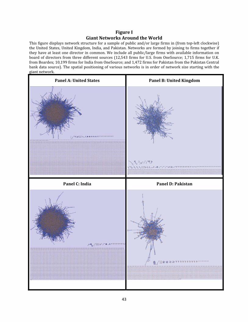
43  

Figure I Giant Networks Around the World  

This figure displays network structure for a sample of public and/or large firms in (from top‐left clockwise) the United States, United Kingdom, India, and Pakistan. Networks are formed by joining to firms together if they have at  least one director  in common. We  include all public/large  firms with available  information on board of directors  from three different sources (12,543  firms  for U.S.  from OneSource; 1,715  firms  for U.K. from Boardex; 10,199 firms for India from OneSource; and 1,472 firms for Pakistan from the Pakistan Central bank data source). The spatial positioning of various networks is  in order of network size starting with the giant network.  

Panel A: United States   Panel B: United Kingdom 

Panel C: India 

 

 

Panel D: Pakistan 

44  

Figure II Network Construction 

This  figure  illustrates  the hypothetical  construction of  a  network.  There  are  eight  firms  in  the  example  (A through  H),  and  a  total  of  fifteen  directors  sitting  on  the  boards  of  these  firms  (labeled  1  through  15). Interlocked board linkages produce two distinct networks and two firms (G and H) that are not connected to anyone else. The largest network consists of Firms A through D, where Firms A, B, and C are linked to each other directly and Firm D is linked to Firms A and B indirectly through its direct link with Firm C. Thus, firms in the same network may be linked to each other through chains of indirect links.  

.  

 

12, 13

G1, 2, 3

A

14, 15

H1, 4,5

C

5,6

D

7,8,9,10

E

2, 3, 4

B

8,9,10

F

2

3

45  

Figure III Giant­Network Structure 

The top panel displays the structure of the giant network. Firms that always remain inside the giant network are represented by black dots, while firms that enter and/or exit the giant network during our sample period are represented by red dots. Firm are linked if they share a common director. The bottom‐left panel provides a  zoom  view  near  the  “core”  of  the  giant  network.  The  bottom‐right  panel  provides  a  zoom  view  of  the peripheral area of the giant network, where firms have fewer connections to other firms than they do near the  “core.” Each node represents a  firm, and  the numbers  inside  indicate  the number of  firms  that node  is connected to.  

Panel A: Giant­Network Structure 

 

Panel B: Core of Giant Network  Panel C: Periphery of Giant Network 

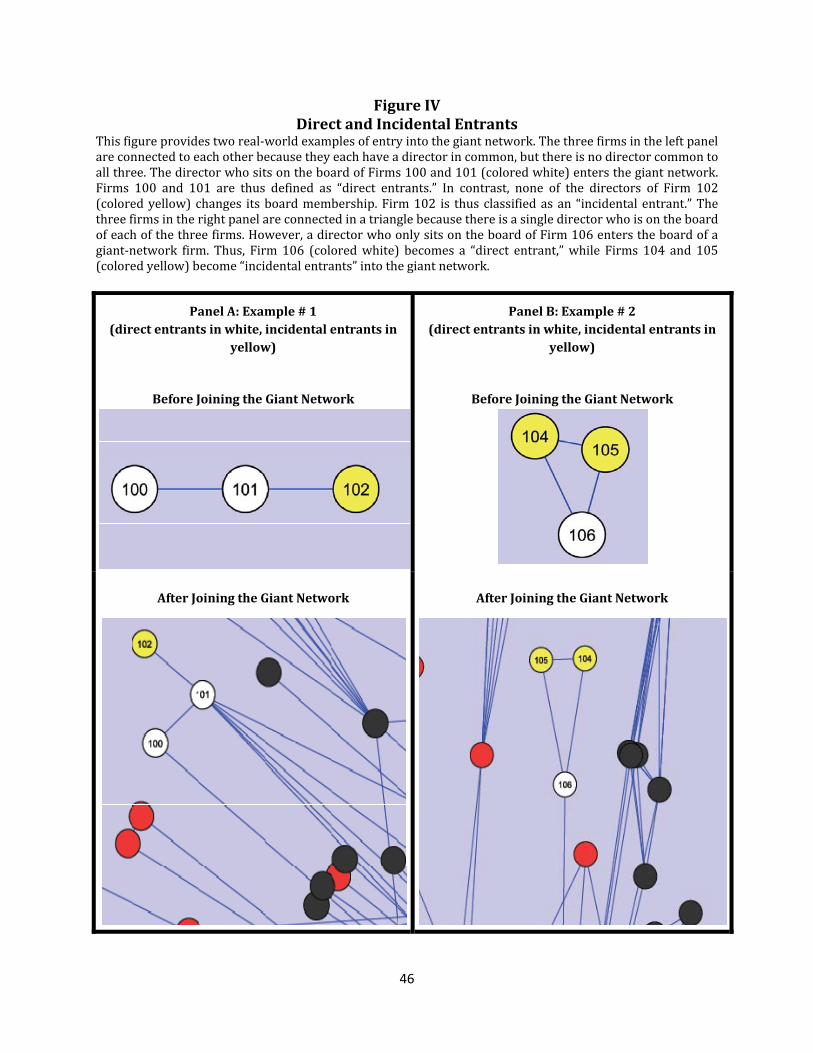
46  

Figure IV Direct and Incidental Entrants 

This figure provides two real‐world examples of entry into the giant network. The three firms in the left panel are connected to each other because they each have a director in common, but there is no director common to all three. The director who sits on the board of Firms 100 and 101 (colored white) enters the giant network. Firms  100  and  101  are  thus  defined  as  “direct  entrants.”  In  contrast,  none  of  the  directors  of  Firm  102 (colored yellow) changes  its board membership. Firm 102  is  thus classified as an  “incidental entrant.” The three firms in the right panel are connected in a triangle because there is a single director who is on the board of each of the three firms. However, a director who only sits on the board of Firm 106 enters the board of a giant‐network  firm.  Thus,  Firm 106  (colored white)  becomes  a  “direct  entrant,” while  Firms  104  and  105 (colored yellow) become “incidental entrants” into the giant network.  

Panel A: Example # 1 (direct entrants in white, incidental entrants in 

yellow) 

 

Before Joining the Giant Network 

Panel B: Example # 2 (direct entrants in white, incidental entrants in 

yellow) 

 

Before Joining the Giant Network 

  

After Joining the Giant Network  

 After Joining the Giant Network 

 

 

47  

Figure V Sample Networked Firms Out of Giant Network 

The  top panel displays network structures of  firms  that enter  the giant network during our  sample period when  they are not  in  the giant network. We picked a  few samples  from different network sizes. The  lower panel repeats the exercise but for firms that never enter the giant network during our sample period. 

  

Panel A: Sample Networks When Not in the Giant Network  

 Panel B: Sample Networks That Never Join the Giant Network 

 

     

48  

Figure VI Effect of Giant­Network Membership: Bank Credit and Financial Distress 

The top panel shows the log of total firm credit from the banking sector as a firm gains entry into the giant network.  The bottom panel  does  the  same  for default  rate. We  follow a  firm  that  enters or  exits  the  giant network once during our sample period, and take out economy‐wide aggregate shocks.   

 

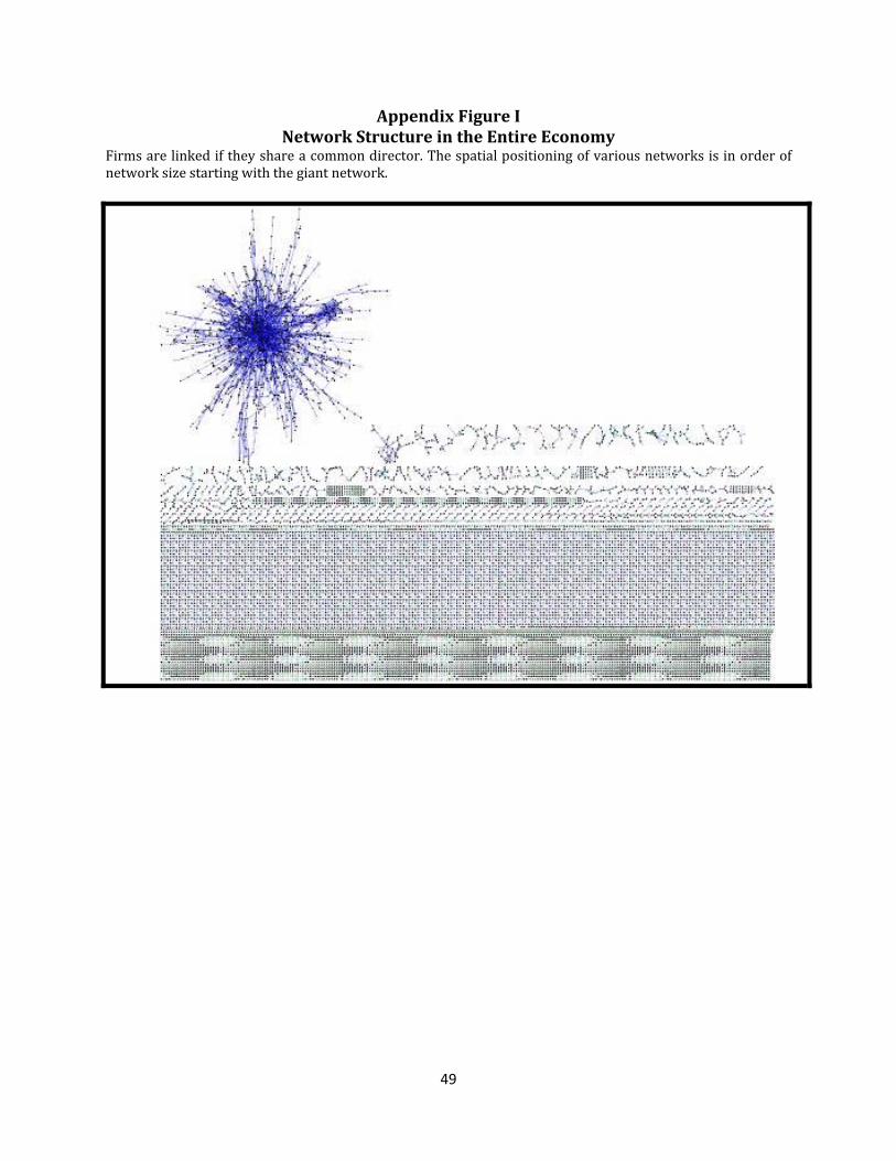
49  

Appendix Figure I Network Structure in the Entire Economy  

Firms are linked if they share a common director. The spatial positioning of various networks is in order of network size starting with the giant network.  

    

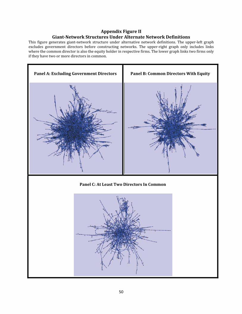
50  

Appendix Figure II Giant­Network Structures Under Alternate Network Definitions 

This  figure  generates  giant‐network  structure  under  alternative  network  definitions.  The  upper‐left  graph excludes  government  directors  before  constructing  networks.  The  upper‐right  graph  only  includes  links where the common director is also the equity holder in respective firms. The lower graph links two firms only if they have two or more directors in common.  

 Panel A: Excluding Government Directors 

 

 Panel B: Common Directors With Equity 

 

 Panel C: At Least Two Directors In Common 

 

 

51  

Appendix Figure III Neighbor Expansion from a Single Starting Node  

Panel A gives a starting node that has 6 immediate neighbors. Subsequent neighbors are indicated in yellow. Panel A 

 

Panel B: Radius = 1 

 

Panel C: Radius = 2 

 

Panel D: Radius = 3 

 Panel E: Radius = 4 

 

Panel F: Radius = 5