Embed Size (px)
Citation preview

Code of Practice
CODE OF PRACTICE 2007 CODE OF PRACTICE 2007 CODE OF PRACTICE 2007 CODE OF PRACTICE 2007 CODE OFPRACTICE 2007 CODE OF PRACTICE 2007 CODE OF PRACTICE 2007 CODE OF PRACTICE 2007 CODE OF PRACTICE 2007CODE OF PRACTICE 2007 CODE OF PRACTICE 2007 CODE OF PRACTICE 2007 CODE OF PRACTICE 2007 CODE OFPRACTICE 2007 CODE OF PRACTICE 2007 CODE OF PRACTICE 2007 CODE OF PRACTICE 2007 CODE OF PRACTICE 2007CODE OF PRACTICE 2007 CODE OF PRACTICE 2007 CODE OF PRACTICE 2007 CODE OF PRACTICE 2007 CODE OFPRACTICE 2007 CODE OF PRACTICE 2007 CODE OF PRACTICE 2007 CODE OF PRACTICE 2007 CODE OF PRACTICE 2007CODE OF PRACTICE 2007 CODE OF PRACTICE 2007 CODE OF PRACTICE 2007 CODE OF PRACTICE 2007 CODE OFPRACTICE 2007 CODE OF PRACTICE 2007 CODE OF PRACTICE 2007 CODE OF PRACTICE 2007 CODE OF PRACTICE 2007CODE OF PRACTICE 2007 CODE OF PRACTICE 2007 CODE OF PRACTICE 2007 CODE OF PRACTICE 2007 CODE OFPRACTICE 2007 CODE OF PRACTICE 2007 CODE OF PRACTICE 2007 CODE OF PRACTICE 2007 CODE OF PRACTICE 2007CODE OF PRACTICE 2007 CODE OF PRACTICE 2007 CODE OF PRACTICE 2007 CODE OF PRACTICE 2007 CODE OFPRACTICE 2007 CODE OF PRACTICE 2007 CODE OF PRACTICE 2007 CODE OF PRACTICE 2007 CODE OF PRACTICE 2007CODE OF PRACTICE 2007 CODE OF PRACTICE 2007 CODE OF PRACTICE 2007 CODE OF PRACTICE 2007 CODE OFPRACTICE 2007 CODE OF PRACTICE 2007 CODE OF PRACTICE 2007 CODE OF PRACTICE 2007 CODE OF PRACTICE 2007CODE OF PRACTICE 2007 CODE OF PRACTICE 2007 CODE OF PRACTICE 2007 CODE OF PRACTICE 2007 CODE OFPRACTICE 2007 CODE OF PRACTICE 2007 CODE OF PRACTICE 2007 CODE OF PRACTICE 2007 CODE OF PRACTICE 2007CODE OF PRACTICE 2007 CODE OF PRACTICE 2007 CODE OF PRACTICE 2007 CODE OF PRACTICE 2007 CODE OFPRACTICE 2007 CODE OF PRACTICE 2007 CODE OF PRACTICE 2007 CODE OF PRACTICE 2007 CODE OF PRACTICE 2007CODE OF PRACTICE 2007 CODE OF PRACTICE 2007 CODE OF PRACTICE 2007 CODE OF PRACTICE 2007 CODE OFPRACTICE 2007 CODE OF PRACTICE 2007 CODE OF PRACTICE 2007 CODE OF PRACTICE 2007 CODE OF PRACTICE 2007CODE OF PRACTICE 2007 CODE OF PRACTICE 2007 CODE OF PRACTICE 2007 CODE OF PRACTICE 2007 CODE OFPRACTICE 2007 CODE OF PRACTICE 2007 CODE OF PRACTICE 2007 CODE OF PRACTICE 2007 CODE OF PRACTICE 2007CODE OF PRACTICE 2007 CODE OF PRACTICE 2007 CODE OF PRACTICE 2007 CODE OF PRACTICE 2007 CODE OFPRACTICE 2007 CODE OF PRACTICE 2007 CODE OF PRACTICE 2007 CODE OF PRACTICE 2007 CODE OF PRACTICE 2007CODE OF PRACTICE 2007 CODE OF PRACTICE 2007 CODE OF PRACTICE 2007 CODE OF PRACTICE 2007 CODE OFPRACTICE 2007 CODE OF PRACTICE 2007 CODE OF PRACTICE 2007 CODE OF PRACTICE 2007 CODE OF PRACTICE 2007CODE OF PRACTICE 2007 CODE OF PRACTICE 2007 CODE OF PRACTICE 2007 CODE OF PRACTICE 2007 CODE OFPRACTICE 2007 CODE OF PRACTICE 2007 CODE OF PRACTICE 2007 CODE OF PRACTICE 2007 CODE OF PRACTICE 2007CODE OF PRACTICE 2007 CODE OF PRACTICE 2007 CODE OF PRACTICE 2007 CODE OF PRACTICE 2007 CODE OFPRACTICE 2007 CODE OF PRACTICE 2007 CODE OF PRACTICE 2007 CODE OF PRACTICE 2007 CODE OF PRACTICE 2007CODE OF PRACTICE 2007 CODE OF PRACTICE 2007 CODE OF PRACTICE 2007 CODE OF PRACTICE 2007 CODE OFPRACTICE 2007 CODE OF PRACTICE 2007 CODE OF PRACTICE 2007 CODE OF PRACTICE 2007 CODE OF PRACTICE 2007CODE OF PRACTICE 2007 CODE OF PRACTICE 2007 CODE OF PRACTICE 2007 CODE OF PRACTICE 2007 CODE OFPRACTICE 2007 CODE OF PRACTICE 2007 CODE OF PRACTICE 2007 CODE OF PRACTICE 2007 CODE OF PRACTICE 2007CODE OF PRACTICE 2007 CODE OF PRACTICE 2007 CODE OF PRACTICE 2007 CODE OF PRACTICE 2007 CODE OFPRACTICE 2007 CODE OF PRACTICE 2007 CODE OF PRACTICE 2007 CODE OF PRACTICE 2007 CODE OF PRACTICE 2007CODE OF PRACTICE 2007 CODE OF PRACTICE 2007 CODE OF PRACTICE 2007 CODE OF PRACTICE 2007 CODE OFPRACTICE 2007 CODE OF PRACTICE 2007 CODE OF PRACTICE 2007 CODE OF PRACTICE 2007 CODE OF PRACTICE 2007CODE OF PRACTICE 2007 CODE OF PRACTICE 2007 CODE OF PRACTICE 2007 CODE OF PRACTICE 2007 CODE OFPRACTICE 2007 CODE OF PRACTICE 2007 CODE OF PRACTICE 2007 CODE OF PRACTICE 2007 CODE OF PRACTICE 2007CODE OF PRACTICE 2007 CODE OF PRACTICE 2007 CODE OF PRACTICE 2007 CODE OF PRACTICE 2007 CODE OFPRACTICE 2007 CODE OF PRACTICE 2007 CODE OF PRACTICE 2007 CODE OF PRACTICE 2007 CODE OF PRACTICE 2007CODE OF PRACTICE 2007 CODE OF PRACTICE 2007 CODE OF PRACTICE 2007 CODE OF PRACTICE 2007 CODE OFPRACTICE 2007 CODE OF PRACTICE 2007 CODE OF PRACTICE 2007 CODE OF PRACTICE 2007 CODE OF PRACTICE 2007CODE OF PRACTICE 2007 CODE OF PRACTICE 2007 CODE OF PRACTICE 2007 CODE OF PRACTICE 2007 CODE OFPRACTICE 2007 CODE OF PRACTICE 2007 CODE OF PRACTICE 2007 CODE OF PRACTICE 2007 CODE OF PRACTICE 2007CODE OF PRACTICE 2007 CODE OF PRACTICE 2007 CODE OF PRACTICE 2007 CODE OF PRACTICE 2007 CODE OFPRACTICE 2007 CODE OF PRACTICE 2007 CODE OF PRACTICE 2007 CODE OF PRACTICE 2007 CODE OF PRACTICE 2007CODE OF PRACTICE 2007 CODE OF PRACTICE 2007 CODE OF PRACTICE 2007 CODE OF PRACTICE 2007 CODE OFPRACTICE 2007 CODE OF PRACTICE 2007 CODE OF PRACTICE 2007 CODE OF PRACTICE 2007 CODE OF PRACTICE 2007CODE OF PRACTICE 2007 CODE OF PRACTICE 2007 CODE OF PRACTICE 2007 CODE OF PRACTICE 2007 CODE OFPRACTICE 2007 CODE OF PRACTICE 2007 CODE OF PRACTICE 2007 CODE OF PRACTICE 2007 CODE OF PRACTICE 2007CODE OF PRACTICE 2007 CODE OF PRACTICE 2007 CODE OF PRACTICE 2007 CODE OF PRACTICE 2007 CODE OFPRACTICE 2007 CODE OF PRACTICE 2007 CODE OF PRACTICE 2007 CODE OF PRACTICE 2007 CODE OF PRACTICE 2007CODE OF PRACTICE 2007 CODE OF PRACTICE 2007 CODE OF PRACTICE 2007 CODE OF PRACTICE 2007 CODE OFPRACTICE 2007 CODE OF PRACTICE 2007 CODE OF PRACTICE 2007 CODE OF PRACTICE 2007 CODE OF PRACTICE 2007CODE OF PRACTICE 2007 CODE OF PRACTICE 2007 CODE OF PRACTICE 2007 CODE OF PRACTICE 2007 CODE OFPRACTICE 2007 CODE OF PRACTICE 2007 CODE OF PRACTICE 2007 CODE OF PRACTICE 2007 CODE OF PRACTICE 2007CODE OF PRACTICE 2007 CODE OF PRACTICE 2007 CODE OF PRACTICE 2007 CODE OF PRACTICE 2007 CODE OFPRACTICE 2007 CODE OF PRACTICE 2007 CODE OF PRACTICE 2007 CODE OF PRACTICE 2007 CODE OF PRACTICE 2007
Staff Working Paper No. 816Machine learning explainability in finance: an application to default risk analysisPhilippe Bracke, Anupam Datta, Carsten Jung and Shayak Sen
August 2019
Staff Working Papers describe research in progress by the author(s) and are published to elicit comments and to further debate. Any views expressed are solely those of the author(s) and so cannot be taken to represent those of the Bank of England or to state Bank of England policy. This paper should therefore not be reported as representing the views of the Bank of England or members of the Monetary Policy Committee, Financial Policy Committee or Prudential Regulation Committee.
Staff Working Paper No. 816Machine learning explainability in finance: an application to default risk analysisPhilippe Bracke,(1) Anupam Datta,(2) Carsten Jung(3) and Shayak Sen(4)
Abstract
We propose a framework for addressing the ‘black box’ problem present in some Machine Learning (ML) applications. We implement our approach by using the Quantitative Input Influence (QII) method of Datta et al (2016) in a real‑world example: a ML model to predict mortgage defaults. This method investigates the inputs and outputs of the model, but not its inner workings. It measures feature influences by intervening on inputs and estimating their Shapley values, representing the features’ average marginal contributions over all possible feature combinations. This method estimates key drivers of mortgage defaults such as the loan‑to‑value ratio and current interest rate, which are in line with the findings of the economics and finance literature. However, given the non‑linearity of ML model, explanations vary significantly for different groups of loans. We use clustering methods to arrive at groups of explanations for different areas of the input space. Finally, we conduct simulations on data that the model has not been trained or tested on. Our main contribution is to develop a systematic analytical framework that could be used for approaching explainability questions in real world financial applications. We conclude though that notable model uncertainties do remain which stakeholders ought to be aware of.
Key words: Machine learning, explainability, mortgage defaults.
JEL classification: C55, G21.
(1) UK Financial Conduct Authority. Email: [email protected](2) Carnegie Mellon University. Email: [email protected](3) Bank of England. Email: [email protected](4) Carnegie Mellon University. Email: [email protected]
The views expressed here are not those of the Financial Conduct Authority or the Bank of England. We thank seminar participants at the Bank of England, the MIT Interpretable Machine‑Learning Models and Financial Applications workshop, the UCL Data for Policy Conference, Louise Eggett, Tom Mutton and other colleagues at the Bank of England and Financial Conduct Authority for very useful comments. Datta and Sen’s work was partially supported by the US National Science Foundation under the grant CNS‑1704845.
The Bank’s working paper series can be found at www.bankofengland.co.uk/working‑paper/staff‑working‑papers
Bank of England, Threadneedle Street, London, EC2R 8AH Email [email protected]
© Bank of England 2019 ISSN 1749‑9135 (on‑line)

1 Introduction
Machine learning (ML) based predictive techniques are seeing increased adoption in a number
of domains, including finance. However, due to their complexity, their predictions are often
difficult to explain and validate. This is sometimes referred to as machine learning’s ‘black box’
problem.
It is important to note that even if ML models are available for inspection, their size and
complexity makes it difficult to explain their operation to humans. For example, an ML model
used to predict mortgage defaults may consist of hundreds of large decision trees deployed in
parallel, making it difficult to summarize how the model works intuitively.
Recently a debate has emerged around techniques for making machine learning models more
explainable. Explanations can answer different kinds of questions about a model’s operation
depending on the stakeholder they are addressed to. In the financial context, there are at least
six different types of stakeholders: (i) Developers, i.e. those developing or implementing an ML
application; (ii) 1st line model checkers, i.e. those directly responsible for making sure model
development is of sufficient quality; (iii) management responsible for the application; (iv) 2nd
line model checkers, i.e. staff that, as part of a firm’s control functions, independently check
the quality of model development and deployment; (v) conduct regulators that take an interest
in deployed models being in line with conduct rules and (vi) prudential regulators that take an
interest in deployed models being in line with prudential requirements.
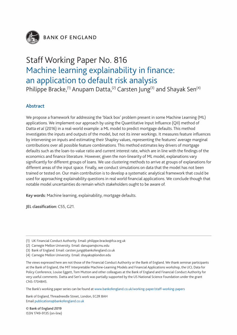
Table 1 outlines the different types of meaningful explanations one could expect for a ma-
chine learning model. A developer may be interested in individual predictions, for instance
when they get customer queries but also to better understand outliers. Similarly, conduct reg-
ulators may occasionally be interested in individual predictions. For instance, if there were
complaints about decisions made, there may be an interest in determining what factors drove
that particular decision. Other stakeholders may be less interested in individual predictions.
For instance, first line model checkers likely would seek a more general understanding of how
the model works and what its key drivers are, across predictions. Similarly, second line model
checkers, management and prudential regulators likely will tend to take a higher level view still.
2
Table 1: Different types of explanationsNote: lighter green means these questions are only partially answered through our approach.
Stakeholder interest1st line 2nd linemodel Manage- model Conduct Prudential
Developer checking ment checking regulator regulator1) Which features mattered inindividual predictions? X X
2) What drove the actualpredictions more generally? X X X X
3) What are the differences betweenthe ML model and a linear one? X X
4) How does the MLmodel work? X X X X X X
5) How will the model performunder new states of the world? X X X X X X(that aren’t captured in the training data)
Especially in cases where a model is of high importance for the business, these stakeholders will
want to make sure the right steps for model quality assurance have been taken and, depending
on the application, they may seek assurance on what the key drivers are.
While regulators expect good model development and governance practices across the board,
the detail and stringency of standards on models vary by application. One area where standards
around model due diligence are most thorough are models used to calculate minimum capital
requirements. Another example is governance requirements around trading and models for
stress testing.1
In this paper, we use one approach to ML explainability, the Quantitative Input Influence
method of [1], which builds on the game-theoretic concept of Shapley values. The QII method
is used in a situation where we observe the inputs of the machine learning model as well as
its outputs, but it would be impractical to examine the internal workings of the model itself.
By changing the inputs in a predetermined way and observing the corresponding changes in
outputs, we can learn about the influence of specific features of the model. By doing so for
several inputs and a large sample of instances, we can draw a useful picture of the model’s
1See for instance https://www.bankofengland.co.uk/-/media/boe/files/prudential-regulation/
supervisory-statement/2018/ss518.
3
functioning. We also demonstrate that input influences can be effectively summarised by using
clustering methods [2]. Hence our approach provides a useful framework for tackling the five
questions outlined in Table 1.
We use this approach in an applied setting: predicting mortgage defaults. For many con-
sumers, mortgages are the most important source of finance, and the estimation of mortgage
default risk has a significant impact on the pricing and availability of mortgages. Recently,
technological innovations—one of which is the application of ML techniques to the estimation
of mortgage default probabilities—have improved the availability of mortgage credit [3]. We
hence use mortgage default predictions as our applied use case. But our explainability approach
can be equally valuable in many other financial applications of machine learning.
We use data on a snapshot of all mortgages outstanding in the United Kingdom and check
their default rates over the subsequent two and a half years. In contrast with some of the most
recent economics literature [4], we are interested in predicting rather than finding the causes of
mortgage defaults. Thus we do not employ techniques or research designs to establish causality
claims as understood in applied economics. Such claims would be necessary for the discussion
of policy interventions. We restrict our exercise to a prediction effort and its explainability,
which is in line with most machine learning applications in the industry. We acknowledge that
there is currently an important debate on making causal inference more prominent in machine
learning.
In a related paper, [5] use a machine learning model to estimate default probabilities in US
data and evaluate the effect of machine learning adoption on the outcomes of different ethnic
groups. Rather than focusing on outcomes such as mortgage pricing or mortgage availability,
in this paper we focus on the estimating process itself and its explainability to relevant parties.
For us, predicting mortgage defaults is just one example of a wide range of problems where ML
explainability techniques can be useful.
The results section of the paper follows Table 1, moving from the particular to the more
general questions. We also examine how explanations change in an out-of-sample setting (in
a simulated stress testing scenario) for logistic regression models and gradient boosted trees,
and find some notable differences. In sum, we find that explainable artificial intelligence (AI)
4

approaches can indeed illuminate which factors were important for making specific predictions
and help understand the logic behind a model’s operation. However, we conclude that some
notable model uncertainties do remain which stakeholders ought to be aware of.
2 Theory: Explaining the functioning of machine learn-
ing models
2.1 Existing approaches to explainability
Explainability has become an active area of research, with several existing approaches.
Naturally, the most straightforward path to explainability is developing a simple, explain-
able model. For instance, linear regression models are considered relatively interpretable, espe-
cially when their regression coefficients have a clear economic meaning. Other models that are
considered as being easy to understand are (small) decision trees or decision rules.
However, in many applied settings it can be advantageous to develop more complex models,
which may require an explainability approach. Such approaches attempt to ‘reverse engineer’
how the workings of the complex model. This means not necessarily trying to explain the model
itself, but to highlight its salient features. There are six ways to do so:
First, one way of reverse engineering a complex ML model is to construct a simpler model
— such as a regression model or small decision tree — that approximates the workings of the
complex one. This is called ‘surrogate model’ [6]. We would refer to this as a ‘global’ model,
as it tries to explain the workings of the complex for all input data.
Second, another global approach is that of Feature Importances, an explainability tech-
nique which has been developed for Random Forest ML models. While it does not build a
surrogate model (that could be used to make predictions) it provides the relative importances
of features for all input data, i.e. on a global level. It does so by estimating the how much
the model prediction variance changes due to the exclusion of individual features. It does not
straightforwardly capture feature interactions.
Third, another option is to build one or several local surrogate models. Local surrogate
5
models approximate the complex model’s predictions on selected sub-sections of the data. In a
mortgage example, one would construct different explainable models for different types of mort-
gage applicants. Such a local approach, is the essence of the Local Interpretable Model-Agnostic
Explanation (LIME) method [7]. Related local approaches are ‘example-based explanations’
which try to explain aspects of a model by focussing on how it classified selected input regions.
Fourth, another approach is to build instance-based explanations. This approach does not
build a ‘model’ (global or local). Rather, it provides explanations on a prediction-by-prediction
basis. It answers questions like ‘what were the driving factors in the case of individual A’?
This is the approach taken by methods which use Shapley values and Individual Conditional
Expectations. The key advantage of Shapley approaches over other instance-based approaches
is that it captures feature-interactions.
Finally, Partial Dependence Plots (PDPs) show the impact of one or two variables have on
the predictive outcome. These are very useful tools to display the non-linearities and other
complexities in the underlying ML model. They are global approaches in the sense that they
are plots that show importances over all the input data. But they are ‘partial’ in the sense that
they can only display one or two features at a time. They also do not consider interactions in
the display on features impact on predictive outcomes.
Our approach is novel in that it combines various elements of the above approaches. By using
a Shapley-based approach, we start out with an instance based approach. We then proceed to
use these to give global explanations. This is similar to a Feature Importances approach, but
allows us to capture interactions between features. Next, we show plots that are conceptual
similar to Partial Dependency Plots, but again are based on Shapley values. This allows us
to show non-linearities, similar to PDPs, yet at the same time capturing feature interactions.
Next, we use also show a local approach which — similar to a local surrogate model approach
— aims to capture the workings of the model on a more granular level.
In this paper, we draw on various of the existing approaches from the explainability toolbox
introduced above and apply them to the ‘5-types-of-explainability’ framework we set out in the
previous section.
6

2.2 Quantitative Input Influence (QII)
As stressed in the previous section, at the heart of our framework developed in this paper is an
instance-based explanation approach - the Quantitative Input Influence (QII) approach. We
outline it in this section, before moving to combining it with other approaches. Traditionally,
influence measures have been studied for feature selection, i.e. informing the choice of which
variables to include in the model [8]. Recently, influence measures have been used as explain-
ability mechanisms [1, 7, 9] for complex models. Influence measures explain the behavior of
models by indicating the relative importance of inputs and their direction. While the space
of potential influence measures is quite large, we point out two requirements that they need
to satisfy: (i) taking into account variable correlations, and (ii) capturing feature interactions.
When inputs to a model tend to move together (e.g. income and loan size), simple measures
of association (such as the correlation between income and defaults) do not distinguish the di-
rection in which each affects outcomes. In complex non-linear classifiers effects arise out of the
interaction between inputs (e.g. if only individuals with high age and high income are deemed
creditworthy), and therefore influence measures should account for these.
QII [1] controls for correlations by employing randomising interventions on inputs, and
accounts for input interactions by measuring the average marginal contributions of inputs over
all sets of features they may interact with. In other words, with this technique, we attempt
various changes of input variables and analyse what changes to output variables they produce.
To see how this works in practice, we focus on the example highlighted in this paper,
mortgage defaults. Suppose we are interested in the influence of a particular input—say, the
borrower’s income—on the probability of default estimated by the model, which becomes our
quantity of interest. (Any property of the system conditional on a particular distribution of
inputs can be a quantity of interest for measuring QII.) In what follows, we start by concen-
trating on individual outcomes, i.e. on questions such as “why was the loan application of this
individual rejected?” or “what would it take for that particular individual to lower their default
probability?”. (These are type-1 explanations according to Table 1.) We will then build up
from these individual-level questions to the the overall functioning of the model, and focus on
7
global questions such as “how important is this input for all individuals that are affected by
the model’s decisions?” (type-2 explanations). These more general questions are especially
relevant for regulators, because they allow an assessment of whether the overall model makes
economic sense and whether it is generally fair towards the people affected by its decisions.
Accounting for input correlations: Unary QII Correlations in data are unavoidable.
Attribution of outcomes in the presence of correlated inputs using associative measures can
result in unsound results. For example, consider the inputs loan size and income that may be
correlated. A model that only uses loan size may yield results that depend on the association
of the income with output, but appear as driven by the loan size alone.
Suppose we want to explain the decision of a machine learning model, or algorithm, A(.),
which takes inputs X = {x1, ..., xn}. To isolate the effect of loan size (xi) on the model out-
come for a specific borrower, we start with a randomising intervention whereby we replace the
individual’s xindi with a value drawn from the distribution of xi in our sample. This intervention
breaks the link between the relevant input and the other inputs of the model, and, if repeated
multiple times, allows us to compute the expected outcome of the model when this input is
randomised, EA(X indi∗ ). The influence of xi, ι(xi), is computed as the difference between the
actual outcome of the model for the individual and the expected outcome of the model when
xi is randomised:
ι(xi) = A(X ind)− EA(X indi∗ ). (1)
In the special case in which the machine learning model happens to be a linear regression,
i.e. A(X) = β0 + β1x1 + ... + βnxn, the expectation term can be carried inside the regression
equation and we have that:
ιlinreg(xi) = βi [xi − E(xi)] . (2)
While limited to a very specific class of models, this equation helps us build intuition around
the two reasons why an input is influential for a given individual: the model put weight on
changes of the input (βi) and the individual is far from the average with respect to that input
(as captured by xi − E(xi)).
8
Accounting for input interactions: Aggregate marginal influence The method de-
scribed above will provide a distorted view of a variable’s influence on the quantity of interest
if, in reality, the effect of the variable on the outcome is channelled through interactions with
other variables. For instance, one might encounter a model in which a low income increases
the likelihood of default only if coupled with a large loan (giving rise to a large loan-to-income
ratio and, depending on the interest rate and maturity of the contract, a high debt-service
ratio). In this case the randomising intervention on loan size alone would not be effective in
identifying the effect of this interaction. It is necessary to intervene on the two variables at the
same time. The principle of the intervention is the same (to replace an input of the model with
a randomised version of it, obtained by drawing from the joint marginal distribution of two or
more features of the model) and the method of evaluating the outcome is the same (i.e., by
focusing on a quantity of interest and deciding how to quantify the distance in the quantity of
interest when the system operates over the real and hypothetical input distributions). In this
case, we speak of joint (or set) QII.
But, going back to the effect of income, how can we make sure that we measure the individual
effect of that variable or, in other words, its true marginal effect? This can be done by taking
the difference between two set QII’s: the one obtained by varying only loan size, and the other
obtained by varying income and loan size together. In this way, we shine a light on the marginal
effect driven by income.
This method naturally leads to another question: given that there are multiple combinations
of possible sets of features, how do we aggregate together all the different marginal contributions
of a variable to construct a measure of aggregate marginal influence, which could be viewed as
the ultimate measure of the influence of a variable? The answer relies on Shapley values.
Shapley values are a concept originally developed in game theory to share the revenues of
a game among all participants [10]. A particular instance of revenue division that has received
attention in this space is the measurement of voting power: how much influence has voter (or
state or constituency) xi on the total outcome? Providing such an answer requires examining
all the possible coalitions that xi can form with other players—which we can indicate as the set∏(X) of all permutations of X. For each of these coalitions, xi can add a marginal contribution
9
(defined as m(xi)) to the final outcome (the result of the vote). The Shapley value of input xi,
which we indicate as ψi, is the expected marginal contribution of that input:
ψi = E[m(xi)] =1
n!
∑∏
(X)
m(xi). (3)
The Shapley value has interesting axiomatic properties that make it a good choice to measure
the aggregate marginal contribution of an input (see [1]). It is also possible to use Shapley
values as a tool to perform statistical inference on machine learning models [11], which falls
outside the scope of the present paper.
Because its foundations lie in the problem of revenue division, the sum of the Shapley values
of all input is equal to the outcome of the model. Taking again the specific (and simplified)
example of a linear regression (this time including one interaction term), it is easy to see how
this property is verified:
A(X) = β0 + ...+ βixi + βjxj + βij(xi ∗ xj) + ...+ βnxn. (4)
When there are no interactions (i.e., the model does not contain the term βij(xi ∗ xj)), the
Shapley value is just the Unary QII shown in equation (2). The sum of all Unary QII’s for an
observation is equal to the predicted value for that observation, A(X) minus a constant, β0.
In the presence of an interaction term, one needs to check the influence of input xi under all
possible combinations of the other inputs. In a linear regression setting, this task is simplified
by the fact that all inputs except xi and xj have no effect on the influence of xi. Because of
the interaction between xi and xj, the marginal influence of xi depends on the value of xj and
its distribution in the sample.
Global measures of influence When thinking about the global influence of an input on
a machine learning algorithm, it is best to see it as an aggregation over all the individual
influences of this input on the loans or elements of the sample. However, because a given input
will have a positive influence on the classification (or estimated default probability) of some
borrowers and a negative influence on some other borrowers, it is useful to take the absolute
10
value of the influences, or their square, before summing or averaging them. Otherwise, in the
context of a linear regression model, if we were to intervene on an input by reshuffling its values
across all the individuals in the sample, we would end up with an overall effect of zero on the
average prediction.
2.3 Global cluster explanations
The QII approach allows us to identify the features that are most relevant for the model’s
estimation of default probabilities. We then use this insight to cluster the mortgages in our
population based on these important features, ending up with an intuitive characterisation of
how the model discriminates between loans. These global cluster explanations consist of two
parts: clustering on QII explanations, and a succinct cluster description in terms of combina-
tions of features [2].
Clustering methods rely heavily on a suitable distance metric to distinguish between points
that should be considered distant versus points that should be considered adjacent. In this
work, we choose the distance between QII explanations as a distance metric for clustering. The
intuition behind the use explanation space for clustering is that explanations suitably raise the
importance of important features and suppress the importance of the features unimportant for
the prediction task at hand. For example, consider a linear model with input vector X, where
each xi is uniformly distributed on {−1, 1}. Clustering on the feature space will lead to 2n
clusters. However, the QII of each feature xi will be βixi. If for any individual most βi’s are
small, then one would expect a smaller number of explanation clusters corresponding to high
βi’s.
3 Data
For our analysis we use data on the universe of outstanding UK regulated mortgages collected by
the UK Financial Conduct Authority (FCA). Starting from June 2015, this dataset is updated
every six months and contains information on loan characteristics (e.g. original and current
balance, type of mortgage, current interest rate) and performance (e.g. whether the loan was
11
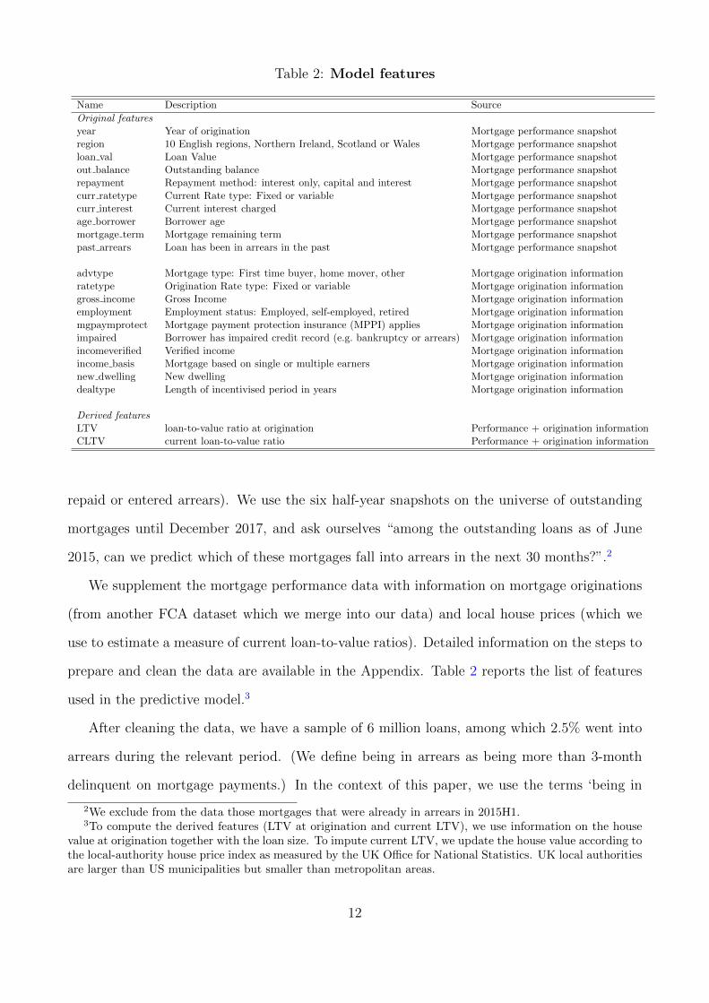
Table 2: Model features
Name Description Source
Original featuresyear Year of origination Mortgage performance snapshotregion 10 English regions, Northern Ireland, Scotland or Wales Mortgage performance snapshotloan val Loan Value Mortgage performance snapshotout balance Outstanding balance Mortgage performance snapshotrepayment Repayment method: interest only, capital and interest Mortgage performance snapshotcurr ratetype Current Rate type: Fixed or variable Mortgage performance snapshotcurr interest Current interest charged Mortgage performance snapshotage borrower Borrower age Mortgage performance snapshotmortgage term Mortgage remaining term Mortgage performance snapshotpast arrears Loan has been in arrears in the past Mortgage performance snapshot
advtype Mortgage type: First time buyer, home mover, other Mortgage origination informationratetype Origination Rate type: Fixed or variable Mortgage origination informationgross income Gross Income Mortgage origination informationemployment Employment status: Employed, self-employed, retired Mortgage origination informationmgpaymprotect Mortgage payment protection insurance (MPPI) applies Mortgage origination informationimpaired Borrower has impaired credit record (e.g. bankruptcy or arrears) Mortgage origination informationincomeverified Verified income Mortgage origination informationincome basis Mortgage based on single or multiple earners Mortgage origination informationnew dwelling New dwelling Mortgage origination informationdealtype Length of incentivised period in years Mortgage origination information
Derived featuresLTV loan-to-value ratio at origination Performance + origination informationCLTV current loan-to-value ratio Performance + origination information
repaid or entered arrears). We use the six half-year snapshots on the universe of outstanding
mortgages until December 2017, and ask ourselves “among the outstanding loans as of June
2015, can we predict which of these mortgages fall into arrears in the next 30 months?”.2
We supplement the mortgage performance data with information on mortgage originations
(from another FCA dataset which we merge into our data) and local house prices (which we
use to estimate a measure of current loan-to-value ratios). Detailed information on the steps to
prepare and clean the data are available in the Appendix. Table 2 reports the list of features
used in the predictive model.3
After cleaning the data, we have a sample of 6 million loans, among which 2.5% went into
arrears during the relevant period. (We define being in arrears as being more than 3-month
delinquent on mortgage payments.) In the context of this paper, we use the terms ‘being in
2We exclude from the data those mortgages that were already in arrears in 2015H1.3To compute the derived features (LTV at origination and current LTV), we use information on the house
value at origination together with the loan size. To impute current LTV, we update the house value according tothe local-authority house price index as measured by the UK Office for National Statistics. UK local authoritiesare larger than US municipalities but smaller than metropolitan areas.
12
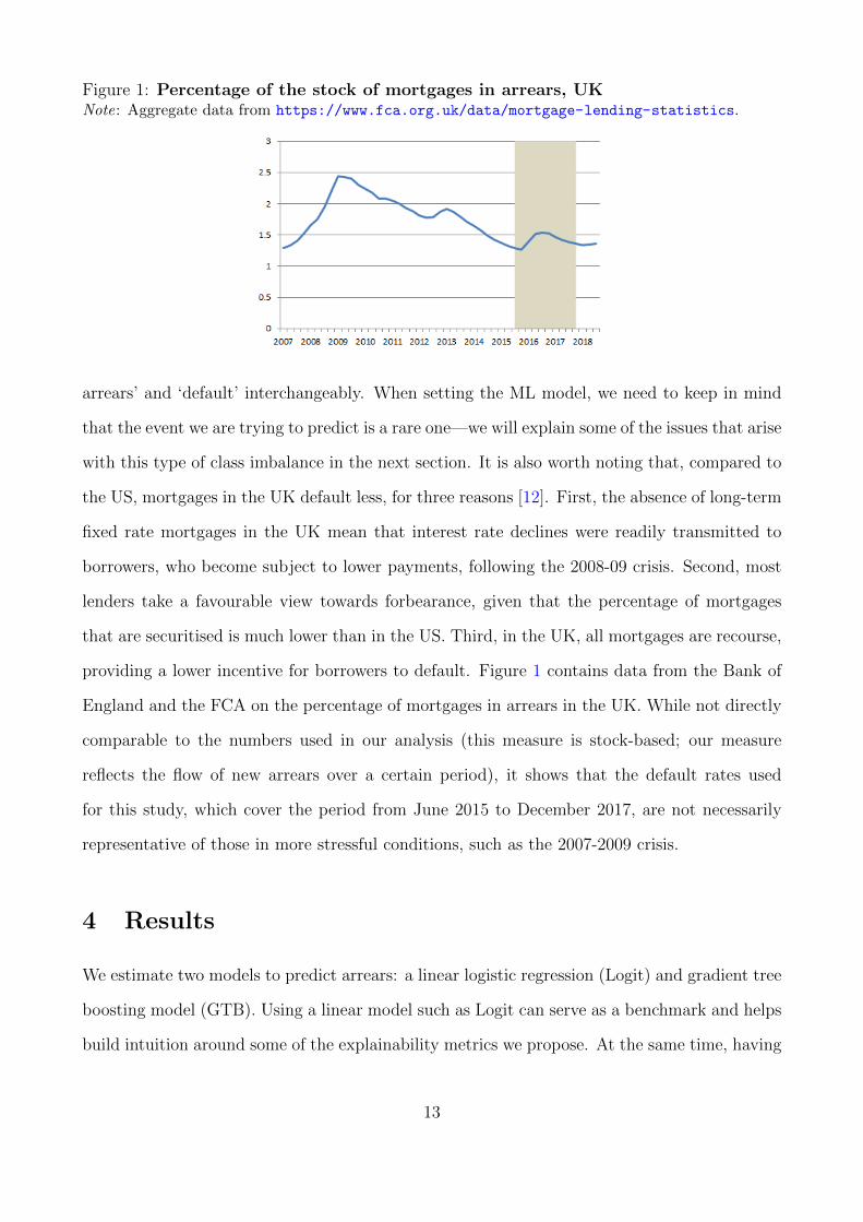
Figure 1: Percentage of the stock of mortgages in arrears, UKNote: Aggregate data from https://www.fca.org.uk/data/mortgage-lending-statistics.
arrears’ and ‘default’ interchangeably. When setting the ML model, we need to keep in mind
that the event we are trying to predict is a rare one—we will explain some of the issues that arise
with this type of class imbalance in the next section. It is also worth noting that, compared to
the US, mortgages in the UK default less, for three reasons [12]. First, the absence of long-term
fixed rate mortgages in the UK mean that interest rate declines were readily transmitted to
borrowers, who become subject to lower payments, following the 2008-09 crisis. Second, most
lenders take a favourable view towards forbearance, given that the percentage of mortgages
that are securitised is much lower than in the US. Third, in the UK, all mortgages are recourse,
providing a lower incentive for borrowers to default. Figure 1 contains data from the Bank of
England and the FCA on the percentage of mortgages in arrears in the UK. While not directly
comparable to the numbers used in our analysis (this measure is stock-based; our measure
reflects the flow of new arrears over a certain period), it shows that the default rates used
for this study, which cover the period from June 2015 to December 2017, are not necessarily
representative of those in more stressful conditions, such as the 2007-2009 crisis.
4 Results
We estimate two models to predict arrears: a linear logistic regression (Logit) and gradient tree
boosting model (GTB). Using a linear model such as Logit can serve as a benchmark and helps
build intuition around some of the explainability metrics we propose. At the same time, having
13

a more ‘black-box’ model such as GTB helps us highlight the benefits of our methodology. Also,
the approach we propose is useful to discriminate between models in general, and we show here
how it can be used to develop insight into why some models appear to perform better than
others.
We tried various machine learning classifiers, such as random forest and support vector ma-
chine. We picked the GTB classifier over those other classifiers based on its superior predictive
performance. We chose the hyper-parameters of the GBT model via a grid-search algorithm,
using 3-fold cross validation, optimising for predictive accuracy.
Training and testing the models In line with standard practice, we split the sample in a
training and a test set. These samples are made of randomly-selected mortgages and comprise
70% and 30% of the dataset, respectively. The model is estimated on the training set, but its
predictive performance is assessed on the test set.
There are alternative ways to create the training and test set. While our training and test
sets are drawn from all years in the sample, one could have used the early period as training set
and test the model on the later period. This approach mimics a real-world situation in which a
model is trained on past data and then used to predict the performance of subsequent cohorts
of mortgages. At this stage we have not explored this route, given the relatively short period
covered by our dataset; but it is an avenue for future work when more years of data become
available. (This is the approach of [13], who have access to US mortgage data for the period
1995-2014, and use the last two years of the dataset as test set.)
Predictions To assess the performance of the two models, we start by showing the distribu-
tion of estimated default probabilities in Figure 2.
In this section, we take a vector of estimated default probabilities for the loans in the test
set as the primary outcome of our two models. Panel A of Figure 2 shows these estimated
probabilities. In terms of predicted probabilities of default, the GTB model appears to dis-
criminate somewhat more between borrowers, with the group of very-low default probability or
very-high default probability being more populated than in the case of the logistic regression.4
4Strictly speaking, while the Logit model directly produces default probabilities, the GTB model is geared
14

This pattern is not specific to our dataset or our application; rather, it reflects a fundamental
fact: more accurate predictive models discriminate more between individual instances [3].
Because predicted probabilities cannot be negative, and because the overall incidence of
default in our dataset is low, at 2.5%, most mortgages tend to cluster around very low estimated
probabilities, below two percent. Such compression may be unhelpful if we are interested in
showing the workings of the models and, in particular, how the machine learning algorithms
predict outcomes. A better picture of mortgage differentiation can be given by log odds of the
probabilities (log(
p1−p
)), which can take any value. We show these Logit scores in Panel B of
Figure 2.
To move to a measure of model performance, we need to switch our attention from predicted
probabilities to a predicted classification (i.e. will default versus will not default). We then
compare these classifications with actual outcomes. There are different comparisons that can
be performed, but most of them share the same building block: the counting of true and false
positives, and true and false negatives.
ROC curve The receiver operating characteristics (ROC) curve plots the true positive rate
(‘sensitivity’ or ‘recall’, i.e. how many mortgages that actually defaulted are classified as de-
faulting) against the false positive rate (‘fall-out’, i.e. how many mortgages that did not default
are classified as defaulting) as the discrimination threshold (the predicted default probability
above which a mortgage is classified as default) goes from one to zero.
With a high discrimination threshold, the model identifies few true defaults and creates
few false positives. As the threshold diminishes, more mortgages are classified by the model
as in default—some of these actually defaulted, whereas some of them did not. As we reach a
discrimination threshold of one, all mortgages are classified as default, leading to a true positive
rate and a false positive rate of one.
A random classifier would lay on the 45-degree line, because all true defaults and all mort-
towards producing classifications (i.e. whether loans will default or not default). The estimated probabilitiesfor the GTB model are usually produced by counting the number of predicted defaults in the leaves, where thatspecific loan ends up, of the different trees produced by the algorithm. This probability measure may not bethe optimal one, and there are alternatives (see for instance the related discussion in [3]). However, given thatour focus is on explainability and the different probability measures are unlikely to change the main insights ofthe model, in this paper we stick to the standard measure.
15
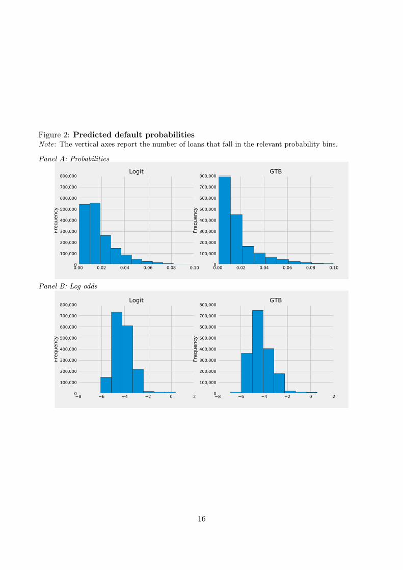
Figure 2: Predicted default probabilitiesNote: The vertical axes report the number of loans that fall in the relevant probability bins.
Panel A: Probabilities
0.00 0.02 0.04 0.06 0.08 0.100
100,000
200,000
300,000
400,000
500,000
600,000
700,000
800,000
Freq
uenc
y
Logit
0.00 0.02 0.04 0.06 0.08 0.100
100,000
200,000
300,000
400,000
500,000
600,000
700,000
800,000
Freq
uenc
y
GTB
Panel B: Log odds
8 6 4 2 0 20
100,000
200,000
300,000
400,000
500,000
600,000
700,000
800,000
Freq
uenc
y
Logit
8 6 4 2 0 20
100,000
200,000
300,000
400,000
500,000
600,000
700,000
800,000
Freq
uenc
y
GTB
16

gages that did not default would have a 50-percent chance of being classified as defaulting.
A good classifier would improve on this random allocation by pushing the curve towards the
top-left corner of the chart, trading off a better recall for any level of fall-out. A commonly used
summary indicator for this is called the area under the curve (AUC), which describes how far
above the 45-degree line the ROC curve is. A 100% AUC indicates perfect predictive accuracy.
The left-hand chart of Figure 3 shows that the greater capacity of the GTB model to
discriminate between ‘good’ and ‘bad’ mortgages appears to lead to better predictions, with
the ROC curve for the GTB model being above the one for the Logit model—we find an AUC
of 81% for the GTB model, compared to 78% for the Logit model.
Precision-recall curve Both recall and fall-out, the two arguments of the ROC curve, do
not directly depend on the actual frequency of the event of interest. With more defaults, for
example, both the numerator and the denominator in recall would rise, and both the numerator
and denominator in fall-out would decrease, leaving the two measures, as well as the ROC curve,
unchanged.
Our application is clearly one in which there are very few observations of the class that
we are aiming to predict (in this case defaults), compared to the other class (non-defaults).
In some models, this could lead the algorithm towards ignoring one class altogether. In other
words, the model may not have sufficient data to learn what actual defaults look like. In such
a situation it might treat the defaulting loans as outliers or totally random events.5 In such a
situation, it might be useful to have an additional metric that focusses on how good the classifier
is at making sure that most of the mortgages identified as defaulting actually defaulted. The
ratio between true positives and all positively-classified observations (true and false positives)
is defined as ‘precision’. The precision-recall curve identifies the trade-offs in datasets with rare
events.
The right-hand side of Figure 3 plots the precision-recall curve for the Logit and GTB
models. Once again, the GTB model appears to offer a better trade-off in terms of predictive
5One way to address this problem is to do ‘oversampling’. In essence, this generates additional syntheticdata of the minority class (in this case defaulting borrowers) in the hope that the model can learn more fromthis additional synthetic data. We tried this, but found that it in our case it did not improve the ROC curve.
17
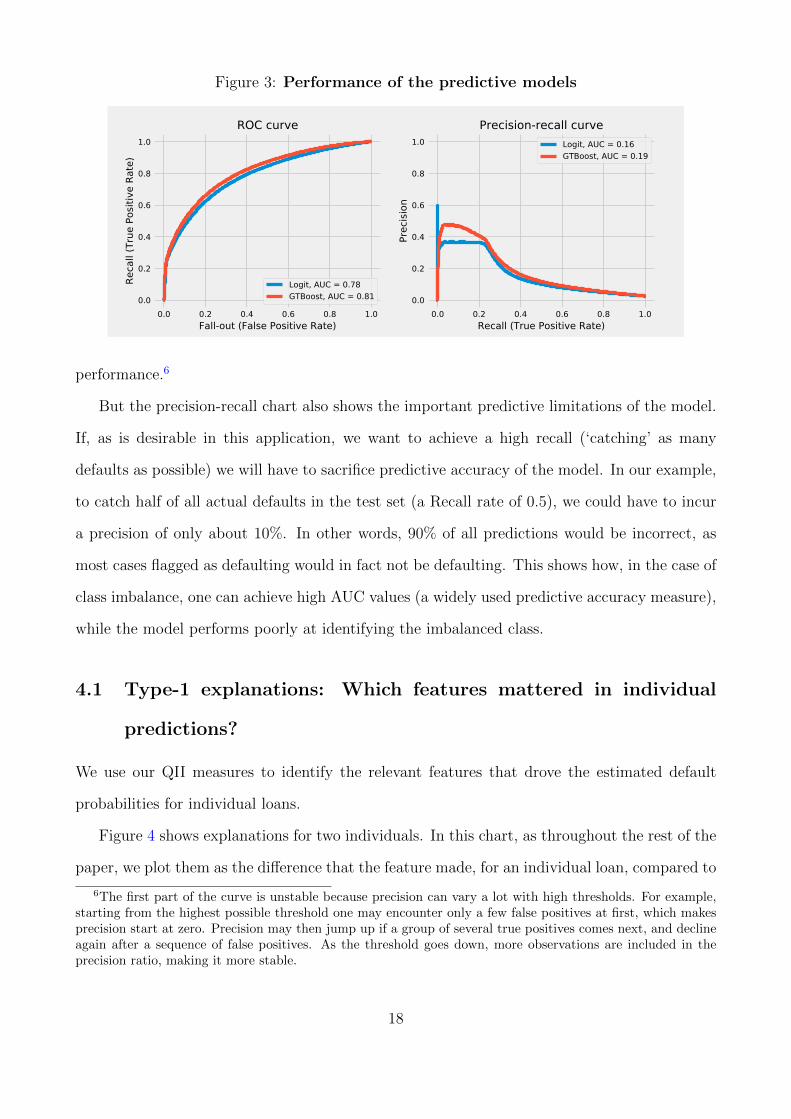
Figure 3: Performance of the predictive models
0.0 0.2 0.4 0.6 0.8 1.0Fall-out (False Positive Rate)
0.0
0.2
0.4
0.6
0.8
1.0Re
call
(Tru
e Po
sitiv
e Ra
te)
ROC curve
Logit, AUC = 0.78GTBoost, AUC = 0.81
0.0 0.2 0.4 0.6 0.8 1.0Recall (True Positive Rate)
0.0
0.2
0.4
0.6
0.8
1.0
Prec
ision
Precision-recall curveLogit, AUC = 0.16GTBoost, AUC = 0.19
performance.6
But the precision-recall chart also shows the important predictive limitations of the model.
If, as is desirable in this application, we want to achieve a high recall (‘catching’ as many
defaults as possible) we will have to sacrifice predictive accuracy of the model. In our example,
to catch half of all actual defaults in the test set (a Recall rate of 0.5), we could have to incur
a precision of only about 10%. In other words, 90% of all predictions would be incorrect, as
most cases flagged as defaulting would in fact not be defaulting. This shows how, in the case of
class imbalance, one can achieve high AUC values (a widely used predictive accuracy measure),
while the model performs poorly at identifying the imbalanced class.
4.1 Type-1 explanations: Which features mattered in individual
predictions?
We use our QII measures to identify the relevant features that drove the estimated default
probabilities for individual loans.
Figure 4 shows explanations for two individuals. In this chart, as throughout the rest of the
paper, we plot them as the difference that the feature made, for an individual loan, compared to
6The first part of the curve is unstable because precision can vary a lot with high thresholds. For example,starting from the highest possible threshold one may encounter only a few false positives at first, which makesprecision start at zero. Precision may then jump up if a group of several true positives comes next, and declineagain after a sequence of false positives. As the threshold goes down, more observations are included in theprecision ratio, making it more stable.
18
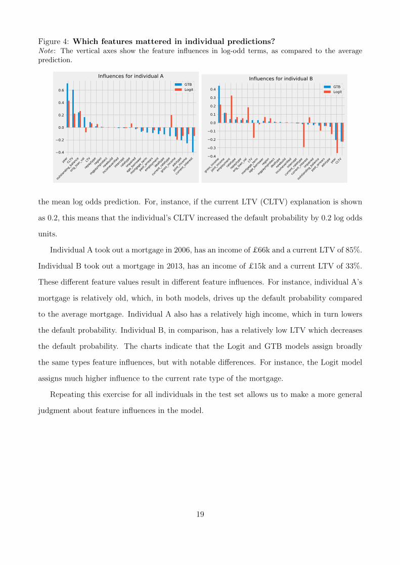
Figure 4: Which features mattered in individual predictions?Note: The vertical axes show the feature influences in log-odd terms, as compared to the averageprediction.
year
CLTV
outst
andin
g_bala
nce
orig_l
oan_v
al LTV
repay
typereg
ion
mgpay
mprotec
t
newbu
ild
incom
everi
fied
interc
ept
ratety
pe
impa
ired
age_b
orrow
er
mortga
ge_te
rm
past_
arrea
rs
emplo
ymen
t
dealt
ype
curren
t_rate
type
gross_
incom
e
advty
pe
joint_in
come
curren
t_inter
est0.4
0.2
0.0
0.2
0.4
0.6
Influences for individual AGTBLogit
gross_
incom
e
joint_in
come
emplo
ymen
t
ratety
pe
repay
type
orig_l
oan_v
al LTV
mortga
ge_te
rm
age_b
orrow
erreg
ion
mgpay
mprotec
t
dealt
ype
newbu
ild
incom
everi
fied
interc
ept
curren
t_rate
type
curren
t_inter
est
impa
ired
outst
andin
g_bala
nce
past_
arrea
rs
advty
pe year
CLTV0.4
0.3
0.2
0.1
0.0
0.1
0.2
0.3
0.4
Influences for individual BGTBLogit
the mean log odds prediction. For, instance, if the current LTV (CLTV) explanation is shown
as 0.2, this means that the individual’s CLTV increased the default probability by 0.2 log odds
units.
Individual A took out a mortgage in 2006, has an income of £66k and a current LTV of 85%.
Individual B took out a mortgage in 2013, has an income of £15k and a current LTV of 33%.
These different feature values result in different feature influences. For instance, individual A’s
mortgage is relatively old, which, in both models, drives up the default probability compared
to the average mortgage. Individual A also has a relatively high income, which in turn lowers
the default probability. Individual B, in comparison, has a relatively low LTV which decreases
the default probability. The charts indicate that the Logit and GTB models assign broadly
the same types feature influences, but with notable differences. For instance, the Logit model
assigns much higher influence to the current rate type of the mortgage.
Repeating this exercise for all individuals in the test set allows us to make a more general
judgment about feature influences in the model.
19
4.2 Type-2 explanations: What drove the explanations more gener-
ally?
We now move to the next two explainability questions from Table 1, which asks for a more
general characterisation of the model. In the first instance, we do this by simply averaging the
absolute values of the individual predictions in the test set.
Similar to the cases of individual A and B above, we find that, on a global level, the Logit
and GTB model end up with a similar ranking of feature influences (see Figure 5). For instance,
variables with high feature influences in both models include the current loan-to-value and loan
interest rate, which are reminiscent of the ‘double-trigger hypothesis’ for mortgage defaults
and in line with findings in the economics literature. According to this view, a borrower would
default only when in negative equity (which is captured by the current LTV), as, for instance,
in the theoretical model of [14]. However, this condition is not sufficient; defaulters are usually
affected by a drop in income or a sudden increase in payments (which in our analysis is captured
by the mortgage interest rate).7 Our findings on the role of LTV and interest rate are consistent
with [16], who also study UK mortgage defaults but use a different data source (mortgages used
as collateral for Bank of England monetary operations).
Therefore, this type of analysis may constitute an important tool for developers who want
to sense-check an opaque ML model against the more transparent results of a Logit regression.
(We report the Logit regression coefficients in Appendix Table A2.)
While the overall ordering of feature influences is sensible, there could nonetheless be poten-
tial oddities that developers and model users would not be able to see without an explainability
lens. For instance, in our application the variable ‘year’ is one of the most influential features
in both models. That is, the older a loan, the more likely is it that a borrower defaults on
it. There may be an economic rationale behind this: for instance, older loans could have been
issued in a time when underwriting standards were laxer. Or, because in the UK older mort-
gages tend to switch to a higher variable rate after the end of the initial incentive period, this
7See [15] for a recent analysis of how changes in mortgage payments affect delinquency rates in the US. Theirpaper uses hybrid adjustable rate mortgages (ARMs), which have fixed payments for a limited number of yearsand then reset to another rate periodically until the loan is repaid. Hybrid ARMs have features similar to themajority of UK mortgages studied here.
20

Figure 5: Global feature influences, using log odds scoresNote: The vertical axes show the mean absolute feature influences in the test set.
year
curre
nt_r
atet
ype
CLTV
curre
nt_in
tere
stou
tsta
ndin
g_ba
lanc
egr
oss_
inco
me
join
t_in
com
ead
vtyp
eLT
Vpa
st_a
rrear
sem
ploy
men
tra
tety
peor
ig_lo
an_v
alag
e_bo
rrowe
rre
payt
ype
regi
onm
ortg
age_
term
impa
ired
deal
type
newb
uild
mgp
aym
prot
ect
inco
mev
erifi
edin
terc
ept0.00
0.05
0.10
0.15
0.20
0.25
0.30
0.35Logit
Logit unaryLogit Shapleys
year
curre
nt_in
tere
stCL
TVgr
oss_
inco
me
curre
nt_r
atet
ype
age_
borro
wer
outs
tand
ing_
bala
nce
join
t_in
com
epa
st_a
rrear
sad
vtyp
eLT
Vre
payt
ype
empl
oym
ent
orig
_loan
_val
mor
tgag
e_te
rmra
tety
pede
alty
pere
gion
impa
ired
mgp
aym
prot
ect
inco
mev
erifi
edne
wbui
ldin
terc
ept0.00
0.05
0.10
0.15
0.20
0.25
0.30
0.35
GTBGTB unaryGTB Shapleys
result could reflect the increased payments affecting those borrowers. But this finding could
also point to a problem with the model, especially when it is deployed to new data. So while
there may be an economic rationale for the influence of the year variable in the test set, one
may want to exclude it in live deployment, because this rationale may not hold universally, in
new conditions. In other words, the explainability tool gives a lens into checking if the model
‘makes sense’ and allows the developer to tweak the data if something is at odds with economic
theory. In the example of the year variable, this may mean excluding it. In other cases it may
mean better investigating why the unexpected influence of a variable has occurred.
4.3 Type-3 explanations: What is the difference to a linear model?
We already alluded above to the difference between the Logit and the GTB models. We propose
that discussing the difference between a linear (benchmark) model and a non-linear model can
be considered as a separate type of explanation.
To do so, in Figure 6, we plot the Logit and GTB models next to each other. The figure
indicates, as mentioned above, that the general ordering of features between the two is highly
similar. However it also points out the differences between the two models, for instance with
regards to the influence of ‘current rate type’ (whether it is a fixed or adjustable rate mortgage)
which is more than twice as important in the Logit model than in the GTB model. Conversely,
21
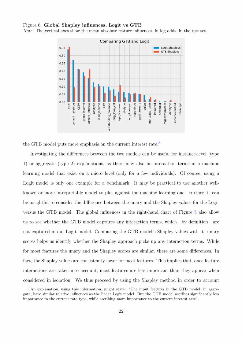
Figure 6: Global Shapley influences, Logit vs GTBNote: The vertical axes show the mean absolute feature influences, in log odds, in the test set.
year
curre
nt_r
atet
ype
CLTV
gros
s_in
com
ecu
rrent
_inte
rest
advt
ype
join
t_in
com
eLT
Vou
tsta
ndin
g_ba
lanc
eor
ig_lo
an_v
alag
e_bo
rrowe
rra
tety
peem
ploy
men
tre
payt
ype
past
_arre
ars
regi
onm
ortg
age_
term
impa
ired
newb
uild
mgp
aym
prot
ect
deal
type
inco
mev
erifi
edin
terc
ept0.00
0.05
0.10
0.15
0.20
0.25
0.30
0.35
Comparing GTB and LogitLogit ShapleysGTB Shapleys
the GTB model puts more emphasis on the current interest rate.8
Investigating the differences between the two models can be useful for instance-level (type
1) or aggregate (type 2) explanations, as there may also be interaction terms in a machine
learning model that exist on a micro level (only for a few individuals). Of course, using a
Logit model is only one example for a benchmark. It may be practical to use another well-
known or more interpretable model to plot against the machine learning one. Further, it can
be insightful to consider the difference between the unary and the Shapley values for the Logit
versus the GTB model. The global influences in the right-hand chart of Figure 5 also allow
us to see whether the GTB model captures any interaction terms, which—by definition—are
not captured in our Logit model. Comparing the GTB model’s Shapley values with its unary
scores helps us identify whether the Shapley approach picks up any interaction terms. While
for most features the unary and the Shapley scores are similar, there are some differences. In
fact, the Shapley values are consistently lower for most features. This implies that, once feature
interactions are taken into account, most features are less important than they appear when
considered in isolation. We thus proceed by using the Shapley method in order to account
8An explanation, using this information, might state: “The input features in the GTB model, in aggre-gate, have similar relative influences as the linear Logit model. But the GTB model ascribes significantly lessimportance to the current rate type, while ascribing more importance to the current interest rate”.
22

for these interactions. As we will show below, such interactions are more clearly visible when
considering input regions of the model. Note that unary and Shapley influences are identical
for a linear model such as Logit, which does not take into account feature interactions if they
are not explicitly built in the model.
4.4 Type-4 explanations: How does the model work?
Mapping feature influences to feature values in the global model Note that Figure 5
purely indicates the relative sizes of influences, not their direction. For instance, it states that
on average year was the most important factor in determining the default probability, more
so than CLTV. However, often for interpreting ‘how the model works’ it is important to also
understand for what type of feature values the influence was higher and for which lower. For
instance, did a high LTV generally increase or decrease default probability in the model? This
type of question is easily answered at the instance or individual level, as shown in Figure 4.
However, because influences that affect some regions of the data do not necessarily translate
into global patterns, a different analysis is needed. To get a sense of the direction of influence,
we need to start mapping the feature values to feature influences. The more comprehensively
and accurately we can do this, the better we understand how the model works for all input
regions of the test set. (The final part of this Results section deals with looking at input regions
that are not in the test set.)
As an initial high-level exercise, we map influences to feature values, by showing their
bivariate correlations, in Table 3. Later years of issuance have a more negative impact on
default probability. In other words, the model finds that more recent mortgages have a lower
likelihood of default. (Note that, from the global influences figure, the direction of influence
could not be inferred given that we looked at absolute values.) The converse seems to be true
for current LTV (CLTV): the higher values of CLTV, the higher their overall impact on default
probability. Higher borrower age is also associated with a higher default probability.
These findings of course rely merely on investigating bivariate correlations. They obscure
non-linearities captured in the model. For instance, in the scatter plots in Figure 7, the CLTV
23
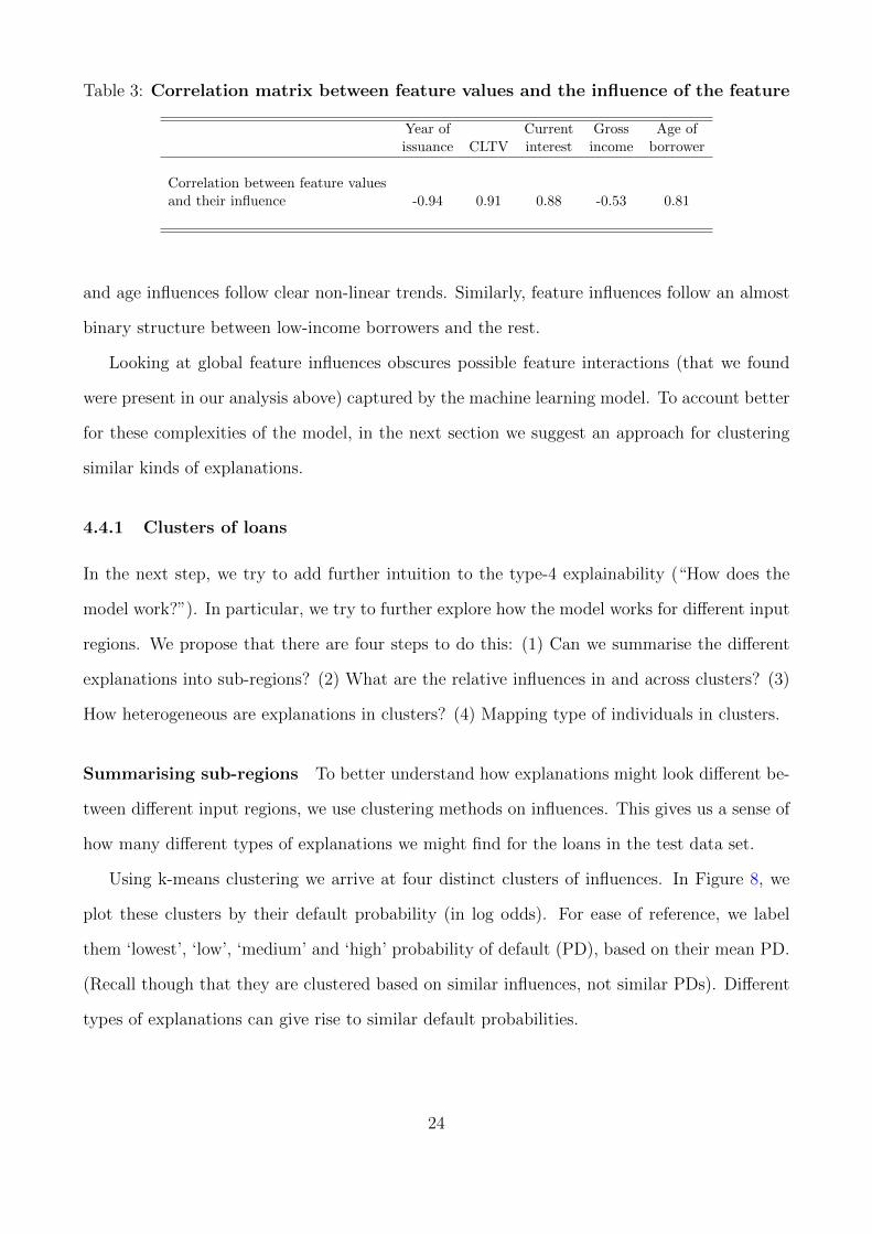
Table 3: Correlation matrix between feature values and the influence of the feature
Year of Current Gross Age ofissuance CLTV interest income borrower
Correlation between feature valuesand their influence -0.94 0.91 0.88 -0.53 0.81
and age influences follow clear non-linear trends. Similarly, feature influences follow an almost
binary structure between low-income borrowers and the rest.
Looking at global feature influences obscures possible feature interactions (that we found
were present in our analysis above) captured by the machine learning model. To account better
for these complexities of the model, in the next section we suggest an approach for clustering
similar kinds of explanations.
4.4.1 Clusters of loans
In the next step, we try to add further intuition to the type-4 explainability (“How does the
model work?”). In particular, we try to further explore how the model works for different input
regions. We propose that there are four steps to do this: (1) Can we summarise the different
explanations into sub-regions? (2) What are the relative influences in and across clusters? (3)
How heterogeneous are explanations in clusters? (4) Mapping type of individuals in clusters.
Summarising sub-regions To better understand how explanations might look different be-
tween different input regions, we use clustering methods on influences. This gives us a sense of
how many different types of explanations we might find for the loans in the test data set.
Using k-means clustering we arrive at four distinct clusters of influences. In Figure 8, we
plot these clusters by their default probability (in log odds). For ease of reference, we label
them ‘lowest’, ‘low’, ‘medium’ and ‘high’ probability of default (PD), based on their mean PD.
(Recall though that they are clustered based on similar influences, not similar PDs). Different
types of explanations can give rise to similar default probabilities.
24
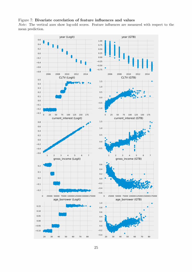
Figure 7: Bivariate correlation of feature influences and valuesNote: The vertical axes show log-odd scores. Feature influences are measured with respect to themean prediction.
2006 2008 2010 2012 20140.8
0.6
0.4
0.2
0.0
0.2
0.4
0.6year (Logit)
2006 2008 2010 2012 2014
0.75
0.50
0.25
0.00
0.25
0.50
0.75
1.00year (GTB)
0 25 50 75 100 125 150 1750.3
0.2
0.1
0.0
0.1
0.2
0.3
0.4
0.5CLTV (Logit)
0 25 50 75 100 125 150 175
1.0
0.5
0.0
0.5
1.0
1.5CLTV (GTB)
1 2 3 4 5 6 70.6
0.4
0.2
0.0
0.2
0.4
0.6
0.8current_interest (Logit)
1 2 3 4 5 6 7
0.5
0.0
0.5
1.0
1.5current_interest (GTB)
0 25000 50000 75000 100000125000150000175000
0.2
0.1
0.0
0.1
0.2
gross_income (Logit)
0 25000 50000 75000 1000001250001500001750000.6
0.4
0.2
0.0
0.2
0.4
0.6
gross_income (GTB)
20 30 40 50 60 70 80
0.10
0.05
0.00
0.05
0.10
0.15
age_borrower (Logit)
20 30 40 50 60 70 800.4
0.2
0.0
0.2
0.4
0.6
0.8
1.0age_borrower (GTB)
25
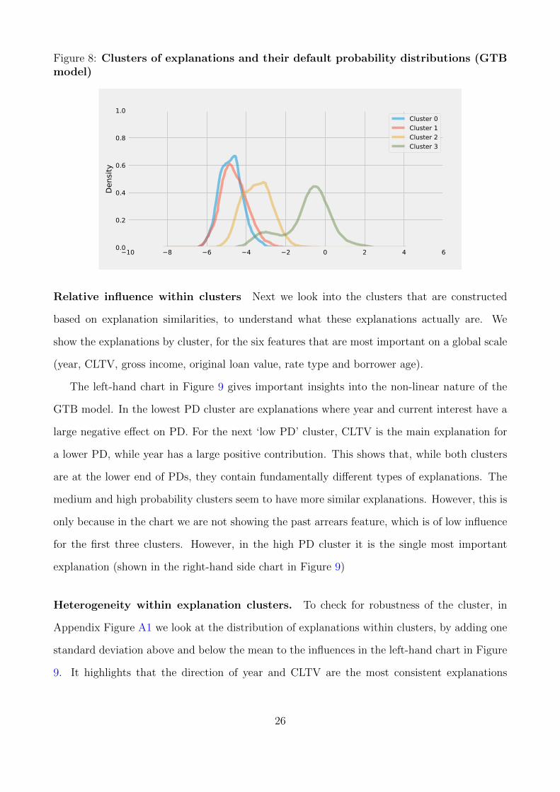
Figure 8: Clusters of explanations and their default probability distributions (GTBmodel)
10 8 6 4 2 0 2 4 60.0
0.2
0.4
0.6
0.8
1.0De
nsity
Cluster 0Cluster 1Cluster 2Cluster 3
Relative influence within clusters Next we look into the clusters that are constructed
based on explanation similarities, to understand what these explanations actually are. We
show the explanations by cluster, for the six features that are most important on a global scale
(year, CLTV, gross income, original loan value, rate type and borrower age).
The left-hand chart in Figure 9 gives important insights into the non-linear nature of the
GTB model. In the lowest PD cluster are explanations where year and current interest have a
large negative effect on PD. For the next ‘low PD’ cluster, CLTV is the main explanation for
a lower PD, while year has a large positive contribution. This shows that, while both clusters
are at the lower end of PDs, they contain fundamentally different types of explanations. The
medium and high probability clusters seem to have more similar explanations. However, this is
only because in the chart we are not showing the past arrears feature, which is of low influence
for the first three clusters. However, in the high PD cluster it is the single most important
explanation (shown in the right-hand side chart in Figure 9)
Heterogeneity within explanation clusters. To check for robustness of the cluster, in
Appendix Figure A1 we look at the distribution of explanations within clusters, by adding one
standard deviation above and below the mean to the influences in the left-hand chart in Figure
9. It highlights that the direction of year and CLTV are the most consistent explanations
26
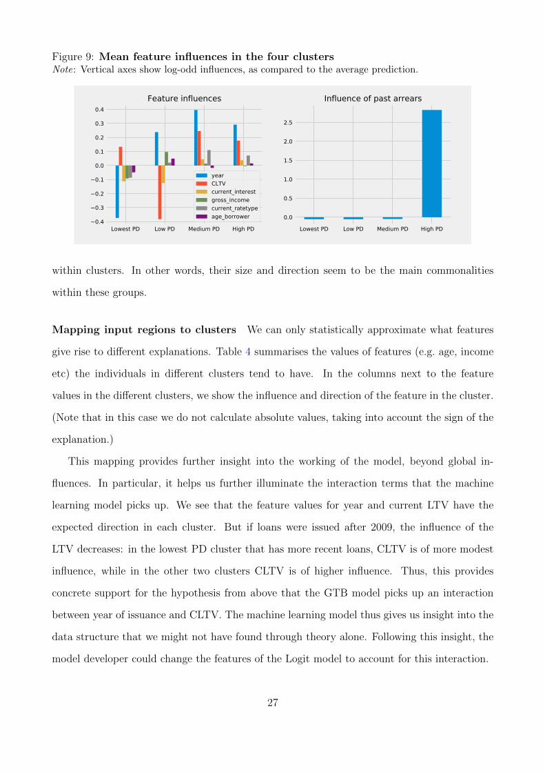
Figure 9: Mean feature influences in the four clustersNote: Vertical axes show log-odd influences, as compared to the average prediction.
Lowest PD Low PD Medium PD High PD0.4
0.3
0.2
0.1
0.0
0.1
0.2
0.3
0.4Feature influences
yearCLTVcurrent_interestgross_incomecurrent_ratetypeage_borrower
Lowest PD Low PD Medium PD High PD0.0
0.5
1.0
1.5
2.0
2.5
Influence of past arrears
within clusters. In other words, their size and direction seem to be the main commonalities
within these groups.
Mapping input regions to clusters We can only statistically approximate what features
give rise to different explanations. Table 4 summarises the values of features (e.g. age, income
etc) the individuals in different clusters tend to have. In the columns next to the feature
values in the different clusters, we show the influence and direction of the feature in the cluster.
(Note that in this case we do not calculate absolute values, taking into account the sign of the
explanation.)
This mapping provides further insight into the working of the model, beyond global in-
fluences. In particular, it helps us further illuminate the interaction terms that the machine
learning model picks up. We see that the feature values for year and current LTV have the
expected direction in each cluster. But if loans were issued after 2009, the influence of the
LTV decreases: in the lowest PD cluster that has more recent loans, CLTV is of more modest
influence, while in the other two clusters CLTV is of higher influence. Thus, this provides
concrete support for the hypothesis from above that the GTB model picks up an interaction
between year of issuance and CLTV. The machine learning model thus gives us insight into the
data structure that we might not have found through theory alone. Following this insight, the
model developer could change the features of the Logit model to account for this interaction.
27
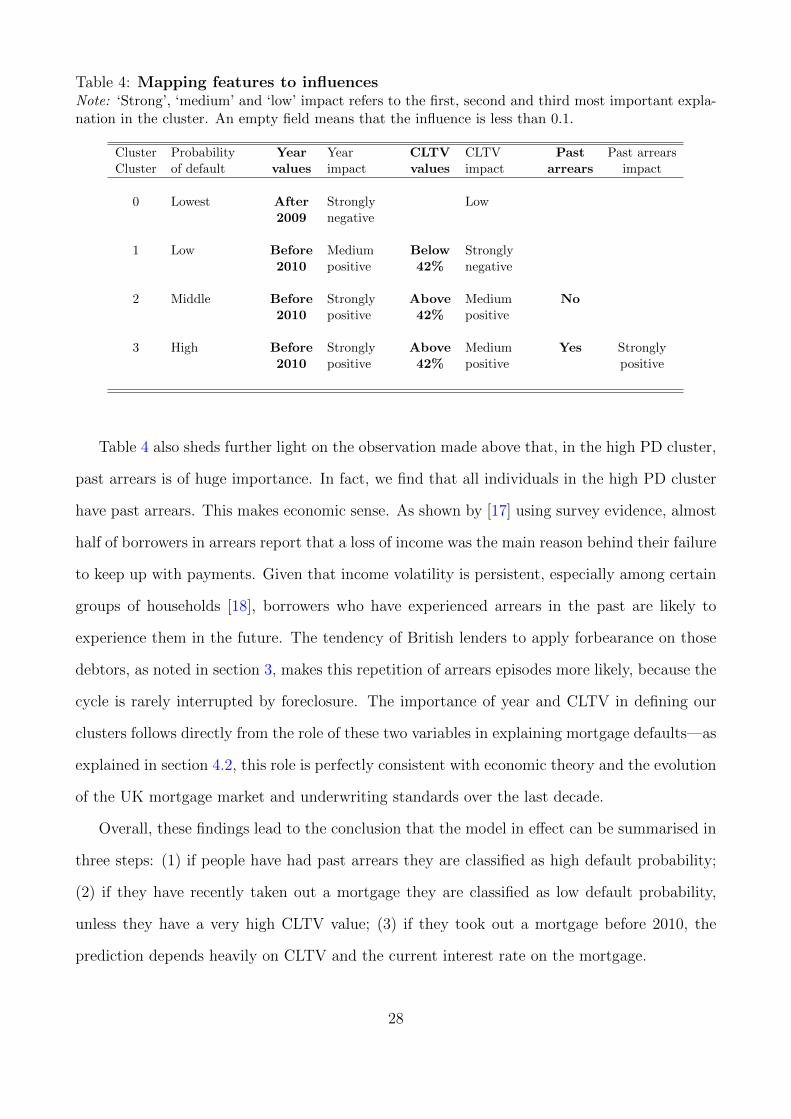
Table 4: Mapping features to influencesNote: ‘Strong’, ‘medium’ and ‘low’ impact refers to the first, second and third most important expla-nation in the cluster. An empty field means that the influence is less than 0.1.
Cluster Probability Year Year CLTV CLTV Past Past arrearsCluster of default values impact values impact arrears impact
0 Lowest After Strongly Low2009 negative
1 Low Before Medium Below Strongly2010 positive 42% negative
2 Middle Before Strongly Above Medium No2010 positive 42% positive
3 High Before Strongly Above Medium Yes Strongly2010 positive 42% positive positive
Table 4 also sheds further light on the observation made above that, in the high PD cluster,
past arrears is of huge importance. In fact, we find that all individuals in the high PD cluster
have past arrears. This makes economic sense. As shown by [17] using survey evidence, almost
half of borrowers in arrears report that a loss of income was the main reason behind their failure
to keep up with payments. Given that income volatility is persistent, especially among certain
groups of households [18], borrowers who have experienced arrears in the past are likely to
experience them in the future. The tendency of British lenders to apply forbearance on those
debtors, as noted in section 3, makes this repetition of arrears episodes more likely, because the
cycle is rarely interrupted by foreclosure. The importance of year and CLTV in defining our
clusters follows directly from the role of these two variables in explaining mortgage defaults—as
explained in section 4.2, this role is perfectly consistent with economic theory and the evolution
of the UK mortgage market and underwriting standards over the last decade.
Overall, these findings lead to the conclusion that the model in effect can be summarised in
three steps: (1) if people have had past arrears they are classified as high default probability;
(2) if they have recently taken out a mortgage they are classified as low default probability,
unless they have a very high CLTV value; (3) if they took out a mortgage before 2010, the
prediction depends heavily on CLTV and the current interest rate on the mortgage.
28
The three steps that summarise the default predictions give stakeholders a good sense of the
overall workings of the model. Importantly, however, these are just attempts to generalise. As
indicated with the error bars in Appendix Figure A1, which shows the ranges of explanations
in clusters, these are still merely averages. In ML models there will likely be a number of
explanations that defy these generalisations. Nonetheless we think that the steps shown above
constitute useful steps in the direction of explaining ‘how the model works’ for the individuals
in the test set. We next turn to explaining how the model works for a hypothetical ‘stress test
set’.
4.5 Type-5 explanations: Testing the model with simulations
Mortgage default models can be used in simulations to understand better how individual assets
and balance sheets perform under stress conditions––for instance, in an economic downturn.
We thus turn to analysing how the model predictions of our Logit and ML models change in
a modified, synthetic test set. Importantly, our goal is to highlight the difference between the
two models, not to say that one is superior to the other.
To do so, we use the assumptions in the Bank of England’s most recent stress-test scenario
for banks, which includes a sharp drop in property prices and a significant increase in unem-
ployment. We then estimate the average default rate, in both models, for this scenario. As
in our original test set, we find more dispersion in the predictions of the ML than the Logit
model as well as a higher average predicted default rate. Finally, we use the QII approach to
bring out what the explanations for predictions were in the stress test scenario. We find that
this explainability method helps shed light on the difference in predictions of the two models.
It again stresses that the ML model explanations vary depending on the input region. This
needs to be taken into account to assess how a model will make predictions in situations that
are significantly different from the training data set, including in tail events.
Background on stress testing. Financial institutions, regulators and central banks have
always been interested in estimating potential losses on their asset portfolios, and how these
losses would affect the balance sheets and ultimately the solvency of financial institutions. After
29

the financial crisis, stress testing has become one of the most prominent approaches to assess
the resilience of the financial system. Stress testing consists of two steps [19]: (i) generation
of stress scenarios, and (ii) stress projections. ML methods can be used in both steps, but in
this paper we focus on the stress projections—for which we employ the model estimated on the
historical data—and take as given the Annual Cyclical Scenario (ACS) proposed by the Bank
of England for its own stress testing exercise.
As described in [20] and [21], the Bank of England uses concurrent stress testing (that is,
stress testing applied to several financial institutions at the same time) to assess the impact
of the adverse scenario on banks’ capital and advance the Bank macro- and microprudential
objectives. Each year the Bank publishes an adverse scenario and asks financial institutions to
submit data and questionnaires related to the impact of the scenario on their balance sheets.
While banks’ submissions constitute the backbone of the exercise, the Bank and other
regulators also carry out their own modelling of the impact of the adverse scenario, as a cross-
check and corroboration of individual submissions. Some of these internal models focus on a
particular sector, such as the owner-occupied mortgage market. The goal of these models is
not to predict the failure of entire institutions (as in [22], for instance); rather, they aim at the
intermediate step of evaluating the effect of the scenario on defaults of individual securities.
This is the context in which we want to test our ML model of mortgage defaults.
While other countries and institutions may have their own particular approach to stress
testing, including specific differences in focus (for example, whether the ultimate goal is an
assessment of the financial health of individual institutions or the whole system), the US Federal
Reserve, the European Banking Authority and the Bank of Japan all have similar procedures.
Constructing the synthetic data for the scenario Given that owner-occupied mortgages
constitute a substantial part of banks’ balance sheets, mortgage arrears and defaults are an
important component of stress testing. We implement our simulation by running the estimated
model on some synthetic data meant to represent the relevant scenario.
Constructing such data is therefore the main preparatory step for this analysis. A scenario
is usually described in terms of macroeconomic variables. The most recent stress test scenario
30
proposed by the Bank of England includes a fall in UK residential property prices of 33%, a
fall in GDP of 4.7%, and an increase in the official Bank Rate to 4%.9
In the simulations presented here, we take the simplifying step of assuming a one-to-one
effect of these variables on the inputs of our model. For some features, such as interest rates,
this assumption does not lead us too far from the actual mechanics of the UK mortgage market.
For instance, a change in Bank Rate would ultimately translate into higher mortgage rates for
all borrowers. (This pass-through would be slowed by the large share of mortgages that are
initially fixed. The fixed-rate period however only last for a limited—two to five—number of
years.) For other variables such as GDP, the impact on borrower-level features such as income
is not straightforward. Reducing every borrower’s income by the same percentage amount,
e.g. 4.7%, would understate the seriousness of the downturn. Economic shocks inflict different
levels of distress to different households, and it is often the most vulnerable people who suffer
the most. An average decline of 4.7% GDP would likely be the result of averaging parts of
the population who suffered no impact together with parts of the population who have suffered
much steeper declines. Because these households are already more likely to default than other
borrowers, an ideal simulation would carefully distribute the shock to different parts of the
population in different magnitudes according to historical experience. At this stage we abstract
from these distributional issues to focus on the main question of extrapolating the results of
machine learning model by feeding them with synthetic inputs, and we restrict the level of
complexity of those input changes. To engineer the scenario mentioned above, we increase the
‘current interest’ feature of our model by 3.5%. (The mortgage characteristics in our sample
refer to June 2015, when the Bank Rate was 0.5%.) We increase all current LTVs by 50% to
reflect the 33% decline in house prices, and reduce all incomes by 5% to incorporate the decline
in GDP.
Simulation findings Applying the scenario above, we find that there are significant dif-
ferences in the stress predictions of the linear and GTB model. Both models predict a shift
towards higher probability of default, but the GTB model more so: the average default prob-
9The Bank of England scenario also includes changes in other variables which, at the moment, we ignore inour simulation.
31
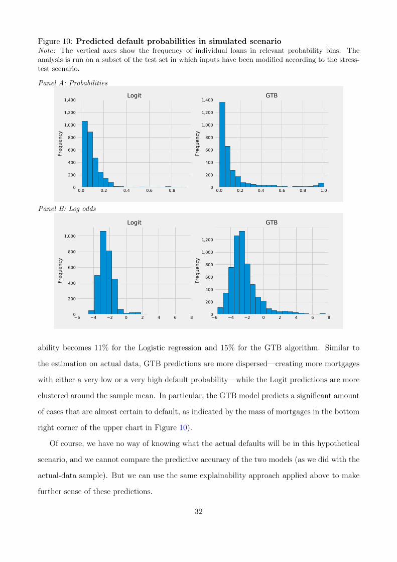
Figure 10: Predicted default probabilities in simulated scenarioNote: The vertical axes show the frequency of individual loans in relevant probability bins. Theanalysis is run on a subset of the test set in which inputs have been modified according to the stress-test scenario.
Panel A: Probabilities
0.0 0.2 0.4 0.6 0.80
200
400
600
800
1,000
1,200
1,400
Freq
uenc
y
Logit
0.0 0.2 0.4 0.6 0.8 1.00
200
400
600
800
1,000
1,200
1,400
Freq
uenc
y
GTB
Panel B: Log odds
6 4 2 0 2 4 6 80
200
400
600
800
1,000
Freq
uenc
y
Logit
6 4 2 0 2 4 6 80
200
400
600
800
1,000
1,200
Freq
uenc
y
GTB
ability becomes 11% for the Logistic regression and 15% for the GTB algorithm. Similar to
the estimation on actual data, GTB predictions are more dispersed—creating more mortgages
with either a very low or a very high default probability—while the Logit predictions are more
clustered around the sample mean. In particular, the GTB model predicts a significant amount
of cases that are almost certain to default, as indicated by the mass of mortgages in the bottom
right corner of the upper chart in Figure 10).
Of course, we have no way of knowing what the actual defaults will be in this hypothetical
scenario, and we cannot compare the predictive accuracy of the two models (as we did with the
actual-data sample). But we can use the same explainability approach applied above to make
further sense of these predictions.
32

Appendix Figure A2 does this and compares aggregate influences between the test and
the simulated data. The influences for the Logit model are identical across test set and the
simulation. This highlights the robustness of the linear model across different input data. It
allows us to explain ex ante how the model works, in terms of relative influences, before we know
which data it is applied to. This is consistent with equation (2) because, with linear models,
the two components of our influence measure are unchanged. The coefficient β remains the
same by definition and, because we created stress-test scenario through a linear transformation
of some inputs for all individuals, the term [x− E(x)] also remains the same for all individuals.
In short, the coefficients and the normalised inputs are unchanged in the simulation.
Conversely, the GTB influences substantially change when the GTB model is applied to the
simulated data. This highlights the general point that machine leaning models often ‘work’ sub-
stantially differently for different input regions, due to non-linearities and interactions between
inputs. For instance, the influence of CLTV and joint income increase substantially—both are
features that drive the simulation. But also features that were not modified in the simulation
see their relative influence change—for instance current interest is less than half as important
as in the test set and original loan value increases about six-fold in influence. Overall, this
means that the ordering of feature influences significantly changes in the simulation.
This highlights the more general point, already outlined in the clustering section, that
explanations for machine learning models can significantly differ between input regions. And
thus explaining the model for a given test is insufficient for explaining it for other input regions.
The upshot of this is that, to make sure the model works as intended under various scenarios,
the developer will have to rely on extensive testing for several potential states of the world,
combined with explainability techniques.
5 Conclusion
In this paper we tackle the explainability problem of AI by studying the inputs and the outputs
of a machine learning model, but not its inner workings. Such a scenario can arise in many
settings, including financial applications; one example could be a mortgage lender with an
33

automated tool to accept or reject loan applications of prospective customers.
The recent literature has offered several approaches to the explainability problem. Here we
employ one that is well suited for a number of financial applications, the QII method of [1], to
derive local and global measures for the influence of a model’s inputs on its outputs. We further
condense the insights from a model by clustering observations with similar input influences.
We demonstrate how to use the QII tools on a gradient tree boosting model of mortgage
defaults, estimated on data comprising all outstanding UK mortgages during the 2015-2017
period.
In the introduction we listed various stakeholders and the types of explanations they may be
interested in. For instance, in the case of a lender which uses a machine learning model to make
its mortgage underwriting decisions, an explainability approach would outline a way to query
the algorithm. By experimenting with multiple application inputs—with features reshuffled in
a methodical way— one could estimate the key drivers of its decisions.
In an alternative example of a different stakeholder, a regulator may be interested in the
workings of machine learning model of mortgage defaults of a bank to assess the riskiness of
its loan book. A regulator could usefully consider an influence-based explainability approach
implemented by the bank. But our paper also highlights that, in this type of situations, it
is still difficult to estimate how a complex model would behave out of sample, for instance in
stress-test scenarios where inputs are deliberately stretched.
In sum, in this paper, we show that explainable AI tools are an important addition to the
data science toolkit, as they allow for better quality assurance of black box ML models. They
can usefully complement other aspects of quality assurance, including various ways of model
performance testing, understanding the properties of the data set and domain knowledge.
34
References
[1] Anupam Datta, Shayak Sen, and Yair Zick. Algorithmic Transparency via Quantitative
Input Influence: Theory and Experiments with Learning Systems. In Proceedings of IEEE
Symposium on Security & Privacy 2016, pages 598–617, 2016.
[2] Anupam Datta and Shayak Sen. Global cluster explanations for machine learning models,
2018. Manuscript.
[3] Andreas Fuster, Matthew Plosser, Philipp Schnabl, and James Vickery. The role of tech-
nology in mortgage lending. Working Paper 24500, National Bureau of Economic Research,
April 2018.
[4] Christopher L Foote and Paul S Willen. Mortgage-default research and the recent foreclo-
sure crisis. Annual Review of Financial Economics, 10:59–100, 2018.
[5] Andreas Fuster, Paul Goldsmith-Pinkham, Tarun Ramadorai, and Ansgar Walther. Pre-
dictably Unequal? The Effects of Machine Learning on Credit Markets. Technical report,
CEPR Discussion Papers, 2017.
[6] Mark Craven and Jude W Shavlik. Extracting tree-structured representations of trained
networks. In Advances in neural information processing systems, pages 24–30, 1996.
[7] Marco Tulio Ribeiro, Sameer Singh, and Carlos Guestrin. “Why Should I Trust You?”:
Explaining the Predictions of Any Classifier. In Proceedings of the 22Nd ACM SIGKDD
International Conference on Knowledge Discovery and Data Mining, KDD ’16, pages 1135–
1144, New York, NY, USA, 2016. ACM.
[8] Leo Breiman. Random forests. Mach. Learn., 45(1):5–32, October 2001.
[9] Scott Lundberg and Su-In Lee. A unified approach to interpreting model predictions.
CoRR, abs/1705.07874, 2017.
[10] Lloyd S Shapley. A value for n-person games. Contributions to the Theory of Games,
2(28):307–317, 1953.
35
[11] Andreas Joseph. Shapley regressions: a framework for statistical inference on machine
learning models. Staff working paper 784, Bank of England, March 2019.
[12] Janine Aron and John Muellbauer. Modelling and forecasting mortgage delinquency and
foreclosure in the uk. Journal of Urban Economics, 94:32–53, 2016.
[13] Justin Sirignano, Apaar Sadhwani, and Kay Giesecke. Deep learning for mortgage risk.
arXiv preprint arXiv:1607.02470, 2016.
[14] John Y Campbell and Joao F Cocco. A model of mortgage default. The Journal of
Finance, 70(4):1495–1554, 2015.
[15] Andreas Fuster and Paul S Willen. Payment size, negative equity, and mortgage default.
American Economic Journal: Economic Policy, 9(4):167–91, 2017.
[16] Vladimir S Lazarov and Marc Hinterschweiger. Determinants of distress in the uk owner-
occupier and buy-to-let mortgage markets. Staff working papers 760, Bank of England,
2018.
[17] Andrew Gall. Understanding mortgage arrears. Technical report, Building Societies Asso-
ciation, 2009.
[18] Karen Dynan, Douglas Elmendorf, and Daniel Sichel. The evolution of household income
volatility. The BE Journal of Economic Analysis & Policy, 12(2), 2012.
[19] Gelin Gao, Bud Mishra, and Daniele Ramazzotti. Causal data science for financial stress
testing. Journal of computational science, 26:294–304, 2018.
[20] Kieran Dent, Ben Westwood, and Miguel Segoviano Basurto. Stress testing of banks: an
introduction. Bank of England Quarterly Bulletin, page Q3, 2016.
[21] Bank of England. Evaluation of the bank of england’s approach to concurrent stress testing.
Technical report, Independent Evaluation Office, 2019.
36

[22] Periklis Gogas, Theophilos Papadimitriou, and Anna Agrapetidou. Forecasting bank fail-
ures and stress testing: A machine learning approach. International Journal of Forecasting,
34(3):440–455, 2018.
[23] Chiranjit Chakraborty, Mariana Gimpelewicz, and Arzu Uluc. A tiger by the tail: esti-
mating the UK mortgage market vulnerabilities from loan-level data. Staff working papers
703, Bank of England, December 2017.
37

Appendix
A Data preparation
We start from the June 2015 snapshot of the universe of outstanding residential mortgages in
the UK, which contains 8,710,173 loans. As shown in Table 2, we need to merge this dataset
with another source (the data on mortgage originations) to add a few relevant variables to our
dataset. In the absence of a unique ID variable shared by the two datasets, we perform the
match sequentially.10 We first look only for those matches that use all the possible common
variables in the two datasets: full postcode, date of birth of the borrower, date in which the
mortgage account was opened, original size of the loan and originating bank. Once we have
performed this first high-quality merge, we drop the requirement that the matched observations
need to share the same originating bank, and perform the match again. We then remove another
variable from the match, original loan amount, and merge again. Finally, we use a less restrictive
match that is based only on full postcode and date of birth of the borrower.
We end up with 6,588,635 mortgages, and we then look for those mortgages in subsequent
snapshots of lenders’ books. Not all mortgages are matched to the subsequent snapshot, either
because the information has been inputed with errors or because the mortgage was genuinely
terminated. This could be because of a sale or a repossession.11
At this stage the sample still contains a wide set of diverse mortgage products; we decide to
drop some of these products given that they differ quite substantially from standard mortgages.
The dropped loans include: lifetime mortgages (a form of equity release), second-charge mort-
gages (these represent only 0.16% of the data), buy-to-let mortgages (these loans for investors
are usually not recorded in the Product Sales Data (PSD); the ones that are reported represent
only 0.03% of the data), shared ownership mortgages (a government scheme whereby a house-
holds partly owns and partly rents a property), shared appreciation mortgages (in which the
borrower pays to the mortgage lender part of the appreciation of the property in exchange for
10This approach is also employed by [23] on the same datasets.11Repossession are preceded by arrears and therefore will be captured by our analysis.
38

an equity release early on), and mortgages to businesses (which are usually not recorded in this
dataset). We also drop mortgages with an initial term of more than 40 years (these are likely
to be mistakes) or less than 5 years (these are uncommon; in fact many lenders require that a
new mortgage has a term of at least 5 years). Similarly, we drop mortgages with an outstand-
ing amount greater than £23m and lower than £1000. These data-cleaning steps reduce the
number of observations to 6,409,213. Finally, a substantial number of loans in the snapshot
are recorded with zero outstanding balance—likely because these mortgages have been repaid
but they are still included in the books. By excluding them the size of the dataset shrinks to
5,834,773 mortgages.
Before running the machine learning predictive model, we prepare the model features, which
are listed in Table 2. We treat the following features as categorical: year, region, advtype, rate-
type, current ratetype, dealtype, repaytype, current interest, and employment. Some features
are zero-one variables: mgpaymprotect, impaired, incomeverified, joint income, newbuild, and
past arrears. For the continuous features in the Logit model, we split the variables into bins to
allow the model to pick up some of the nonlinearities in the data. We split the following vari-
ables: loan size at origination (at £75k, 125k, 175k), current loan size (at £50k, 100k, 150k),
gross income at origination (at £30k, 40k, 60k), LTV at origination (at .5, .7, .85), current
LTV (at .5, .7, .85, .9, .95), mortgage term (at 15, 20, 25), and borrower age (at 30, 40, 50).
39
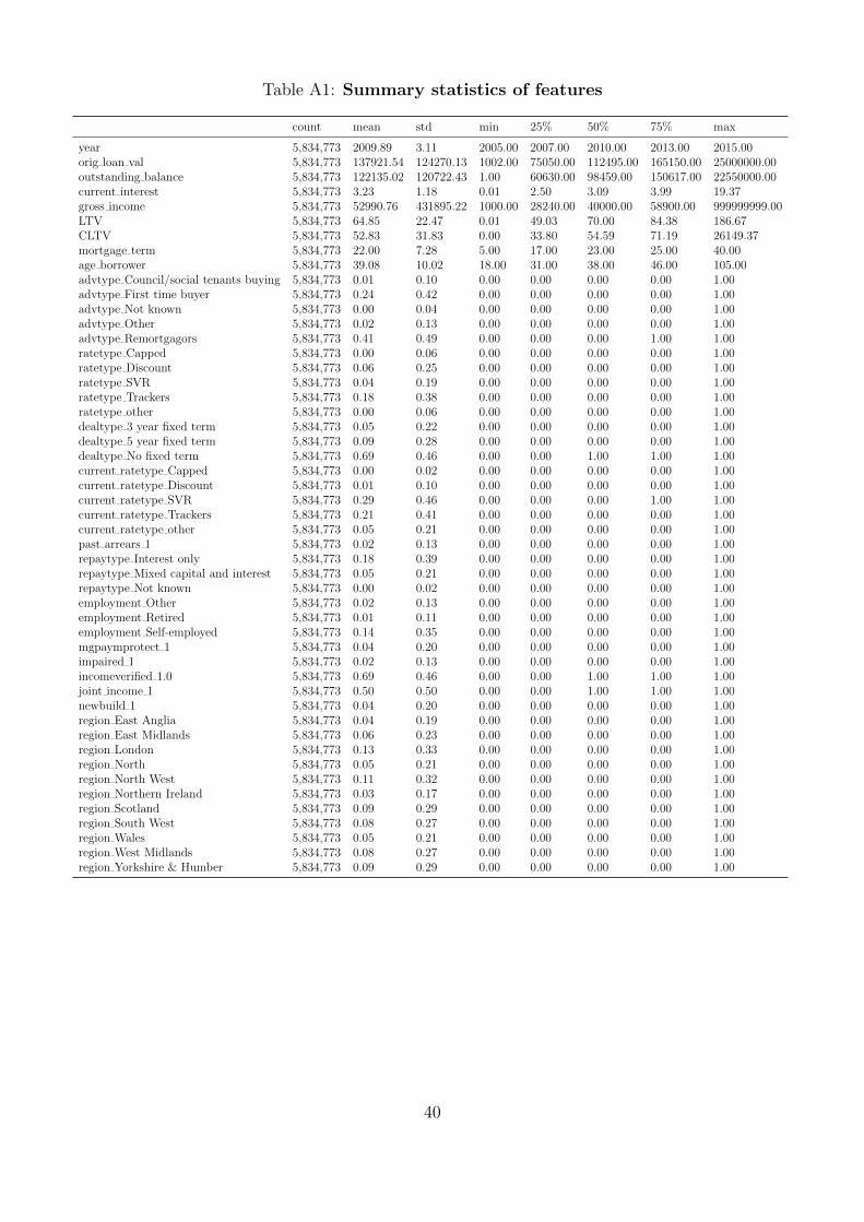
Table A1: Summary statistics of features
count mean std min 25% 50% 75% max
year 5,834,773 2009.89 3.11 2005.00 2007.00 2010.00 2013.00 2015.00orig loan val 5,834,773 137921.54 124270.13 1002.00 75050.00 112495.00 165150.00 25000000.00outstanding balance 5,834,773 122135.02 120722.43 1.00 60630.00 98459.00 150617.00 22550000.00current interest 5,834,773 3.23 1.18 0.01 2.50 3.09 3.99 19.37gross income 5,834,773 52990.76 431895.22 1000.00 28240.00 40000.00 58900.00 999999999.00LTV 5,834,773 64.85 22.47 0.01 49.03 70.00 84.38 186.67CLTV 5,834,773 52.83 31.83 0.00 33.80 54.59 71.19 26149.37mortgage term 5,834,773 22.00 7.28 5.00 17.00 23.00 25.00 40.00age borrower 5,834,773 39.08 10.02 18.00 31.00 38.00 46.00 105.00advtype Council/social tenants buying 5,834,773 0.01 0.10 0.00 0.00 0.00 0.00 1.00advtype First time buyer 5,834,773 0.24 0.42 0.00 0.00 0.00 0.00 1.00advtype Not known 5,834,773 0.00 0.04 0.00 0.00 0.00 0.00 1.00advtype Other 5,834,773 0.02 0.13 0.00 0.00 0.00 0.00 1.00advtype Remortgagors 5,834,773 0.41 0.49 0.00 0.00 0.00 1.00 1.00ratetype Capped 5,834,773 0.00 0.06 0.00 0.00 0.00 0.00 1.00ratetype Discount 5,834,773 0.06 0.25 0.00 0.00 0.00 0.00 1.00ratetype SVR 5,834,773 0.04 0.19 0.00 0.00 0.00 0.00 1.00ratetype Trackers 5,834,773 0.18 0.38 0.00 0.00 0.00 0.00 1.00ratetype other 5,834,773 0.00 0.06 0.00 0.00 0.00 0.00 1.00dealtype 3 year fixed term 5,834,773 0.05 0.22 0.00 0.00 0.00 0.00 1.00dealtype 5 year fixed term 5,834,773 0.09 0.28 0.00 0.00 0.00 0.00 1.00dealtype No fixed term 5,834,773 0.69 0.46 0.00 0.00 1.00 1.00 1.00current ratetype Capped 5,834,773 0.00 0.02 0.00 0.00 0.00 0.00 1.00current ratetype Discount 5,834,773 0.01 0.10 0.00 0.00 0.00 0.00 1.00current ratetype SVR 5,834,773 0.29 0.46 0.00 0.00 0.00 1.00 1.00current ratetype Trackers 5,834,773 0.21 0.41 0.00 0.00 0.00 0.00 1.00current ratetype other 5,834,773 0.05 0.21 0.00 0.00 0.00 0.00 1.00past arrears 1 5,834,773 0.02 0.13 0.00 0.00 0.00 0.00 1.00repaytype Interest only 5,834,773 0.18 0.39 0.00 0.00 0.00 0.00 1.00repaytype Mixed capital and interest 5,834,773 0.05 0.21 0.00 0.00 0.00 0.00 1.00repaytype Not known 5,834,773 0.00 0.02 0.00 0.00 0.00 0.00 1.00employment Other 5,834,773 0.02 0.13 0.00 0.00 0.00 0.00 1.00employment Retired 5,834,773 0.01 0.11 0.00 0.00 0.00 0.00 1.00employment Self-employed 5,834,773 0.14 0.35 0.00 0.00 0.00 0.00 1.00mgpaymprotect 1 5,834,773 0.04 0.20 0.00 0.00 0.00 0.00 1.00impaired 1 5,834,773 0.02 0.13 0.00 0.00 0.00 0.00 1.00incomeverified 1.0 5,834,773 0.69 0.46 0.00 0.00 1.00 1.00 1.00joint income 1 5,834,773 0.50 0.50 0.00 0.00 1.00 1.00 1.00newbuild 1 5,834,773 0.04 0.20 0.00 0.00 0.00 0.00 1.00region East Anglia 5,834,773 0.04 0.19 0.00 0.00 0.00 0.00 1.00region East Midlands 5,834,773 0.06 0.23 0.00 0.00 0.00 0.00 1.00region London 5,834,773 0.13 0.33 0.00 0.00 0.00 0.00 1.00region North 5,834,773 0.05 0.21 0.00 0.00 0.00 0.00 1.00region North West 5,834,773 0.11 0.32 0.00 0.00 0.00 0.00 1.00region Northern Ireland 5,834,773 0.03 0.17 0.00 0.00 0.00 0.00 1.00region Scotland 5,834,773 0.09 0.29 0.00 0.00 0.00 0.00 1.00region South West 5,834,773 0.08 0.27 0.00 0.00 0.00 0.00 1.00region Wales 5,834,773 0.05 0.21 0.00 0.00 0.00 0.00 1.00region West Midlands 5,834,773 0.08 0.27 0.00 0.00 0.00 0.00 1.00region Yorkshire & Humber 5,834,773 0.09 0.29 0.00 0.00 0.00 0.00 1.00
40

Table A2: Coefficients of the logistic regression
Coef. Std.Err. z P>|z| [0.025 0.975]current interest 0.1991 0.0033 60.6934 0.0000 0.1926 0.2055year 2006 -0.0766 0.0133 -5.7590 0.0000 -0.1027 -0.0505year 2007 -0.1746 0.0132 -13.2310 0.0000 -0.2004 -0.1487year 2008 -0.2162 0.0141 -15.2929 0.0000 -0.2439 -0.1885year 2009 -0.3594 0.0173 -20.8020 0.0000 -0.3933 -0.3256year 2010 -0.4798 0.0182 -26.3764 0.0000 -0.5155 -0.4442year 2011 -0.6400 0.0188 -34.0891 0.0000 -0.6768 -0.6032year 2012 -0.8129 0.0197 -41.3607 0.0000 -0.8514 -0.7744year 2013 -0.8736 0.0200 -43.7023 0.0000 -0.9127 -0.8344year 2014 -0.9385 0.0206 -45.5083 0.0000 -0.9790 -0.8981year 2015 -1.2281 0.0308 -39.8749 0.0000 -1.2885 -1.1677advtype Council/social tenants buying 0.3751 0.0273 13.7384 0.0000 0.3215 0.4286advtype First time buyer 0.0939 0.0106 8.8701 0.0000 0.0731 0.1146advtype Not known 0.0945 0.0651 1.4513 0.1467 -0.0331 0.2222advtype Other 0.2173 0.0259 8.3846 0.0000 0.1665 0.2681advtype Remortgagors 0.2614 0.0088 29.8487 0.0000 0.2443 0.2786ratetype Capped -0.4413 0.0756 -5.8374 0.0000 -0.5895 -0.2931ratetype Discount -0.0328 0.0126 -2.5999 0.0093 -0.0576 -0.0081ratetype SVR -0.3750 0.0216 -17.3305 0.0000 -0.4174 -0.3326ratetype Trackers -0.2216 0.0110 -20.1315 0.0000 -0.2431 -0.2000ratetype other -0.6985 0.0884 -7.8979 0.0000 -0.8718 -0.5251current ratetype Capped -0.1430 0.2540 -0.5631 0.5734 -0.6409 0.3549current ratetype Discount 0.2711 0.0362 7.4914 0.0000 0.2002 0.3420current ratetype SVR 0.4819 0.0107 45.1650 0.0000 0.4610 0.5028current ratetype Trackers 0.5590 0.0128 43.6923 0.0000 0.5339 0.5840current ratetype other 0.5461 0.0176 31.0663 0.0000 0.5117 0.5806past arrears 1 2.5915 0.0096 270.4278 0.0000 2.5727 2.6103dealtype 3 year fixed term 0.0189 0.0148 1.2752 0.2023 -0.0101 0.0479dealtype 5 year fixed term -0.1447 0.0150 -9.6272 0.0000 -0.1742 -0.1153dealtype No fixed term -0.0278 0.0093 -3.0027 0.0027 -0.0459 -0.0097repaytype Interest only -0.1546 0.0097 -15.8605 0.0000 -0.1737 -0.1355repaytype Mixed capital and interest -0.4527 0.0195 -23.2029 0.0000 -0.4909 -0.4145repaytype Not known -0.4112 0.1525 -2.6965 0.0070 -0.7101 -0.1123employment Other 0.1814 0.0261 6.9502 0.0000 0.1302 0.2326employment Retired 0.1244 0.0334 3.7208 0.0002 0.0589 0.1899employment Self-employed 0.3776 0.0089 42.2840 0.0000 0.3601 0.3951mgpaymprotect 1 -0.1178 0.0180 -6.5414 0.0000 -0.1532 -0.0825impaired 1 0.5603 0.0148 37.7492 0.0000 0.5313 0.5894incomeverified 1.0 -0.0035 0.0078 -0.4497 0.6530 -0.0187 0.0117joint income 1 -0.2291 0.0074 -31.0131 0.0000 -0.2436 -0.2146newbuild 1 -0.1013 0.0221 -4.5766 0.0000 -0.1448 -0.0579region East Anglia 0.0302 0.0204 1.4776 0.1395 -0.0099 0.0702region East Midlands -0.0255 0.0169 -1.5064 0.1320 -0.0586 0.0077region London 0.0980 0.0135 7.2819 0.0000 0.0716 0.1244region North 0.0403 0.0174 2.3173 0.0205 0.0062 0.0744region North West 0.0942 0.0132 7.1437 0.0000 0.0683 0.1200region Northern Ireland 0.3105 0.0197 15.7664 0.0000 0.2719 0.3491region Scotland 0.0719 0.0144 4.9869 0.0000 0.0436 0.1002region South West -0.0808 0.0160 -5.0490 0.0000 -0.1121 -0.0494region Wales 0.0999 0.0174 5.7458 0.0000 0.0658 0.1340region West Midlands 0.0322 0.0146 2.2072 0.0273 0.0036 0.0608region Yorkshire & Humber 0.0510 0.0142 3.6043 0.0003 0.0233 0.0788orig loan val (75000, 125000] -0.1991 0.0112 -17.7068 0.0000 -0.2211 -0.1771orig loan val (125000, 175000] -0.2710 0.0166 -16.3518 0.0000 -0.3035 -0.2385orig loan val (175000, 10000000] -0.2642 0.0216 -12.2120 0.0000 -0.3066 -0.2218outstanding balance (50000, 100000] 0.2414 0.0129 18.6490 0.0000 0.2161 0.2668outstanding balance (100000, 150000] 0.3929 0.0174 22.5544 0.0000 0.3588 0.4270outstanding balance (150000, 10000000] 0.5994 0.0225 26.6028 0.0000 0.5552 0.6435gross income (30000, 40000] -0.1420 0.0100 -14.1510 0.0000 -0.1617 -0.1224gross income (40000, 60000] -0.3013 0.0117 -25.8123 0.0000 -0.3242 -0.2785gross income (60000, 10000000] -0.4200 0.0149 -28.2107 0.0000 -0.4492 -0.3908LTV (50, 70] 0.1750 0.0127 13.8148 0.0000 0.1502 0.1998LTV (70, 85] 0.2809 0.0145 19.3221 0.0000 0.2524 0.3094LTV (85, 90] 0.2427 0.0173 13.9927 0.0000 0.2087 0.2767LTV (90, 95] 0.3074 0.0194 15.8272 0.0000 0.2693 0.3454LTV (95, 200] 0.3195 0.0232 13.7475 0.0000 0.2740 0.3651CLTV (50, 70] 0.3130 0.0118 26.4967 0.0000 0.2898 0.3361CLTV (70, 85] 0.4340 0.0150 28.9405 0.0000 0.4046 0.4634CLTV (85, 90] 0.5076 0.0213 23.8123 0.0000 0.4659 0.5494CLTV (90, 95] 0.6038 0.0237 25.5202 0.0000 0.5575 0.6502CLTV (95, 100000] 0.6473 0.0213 30.4001 0.0000 0.6056 0.6891mortgage term (15, 20] -0.0780 0.0123 -6.3291 0.0000 -0.1022 -0.0539mortgage term (20, 25] -0.0618 0.0128 -4.8292 0.0000 -0.0869 -0.0367mortgage term (25, 40] -0.1041 0.0156 -6.6841 0.0000 -0.1346 -0.0736age borrower (30, 40] 0.0514 0.0098 5.2544 0.0000 0.0322 0.0705age borrower (40, 50] 0.1692 0.0116 14.5289 0.0000 0.1464 0.1921age borrower (50, 120] 0.2559 0.0156 16.3935 0.0000 0.2253 0.2865intercept -4.9556 0.0286 -173.3582 0.0000 -5.0117 -4.8996
41
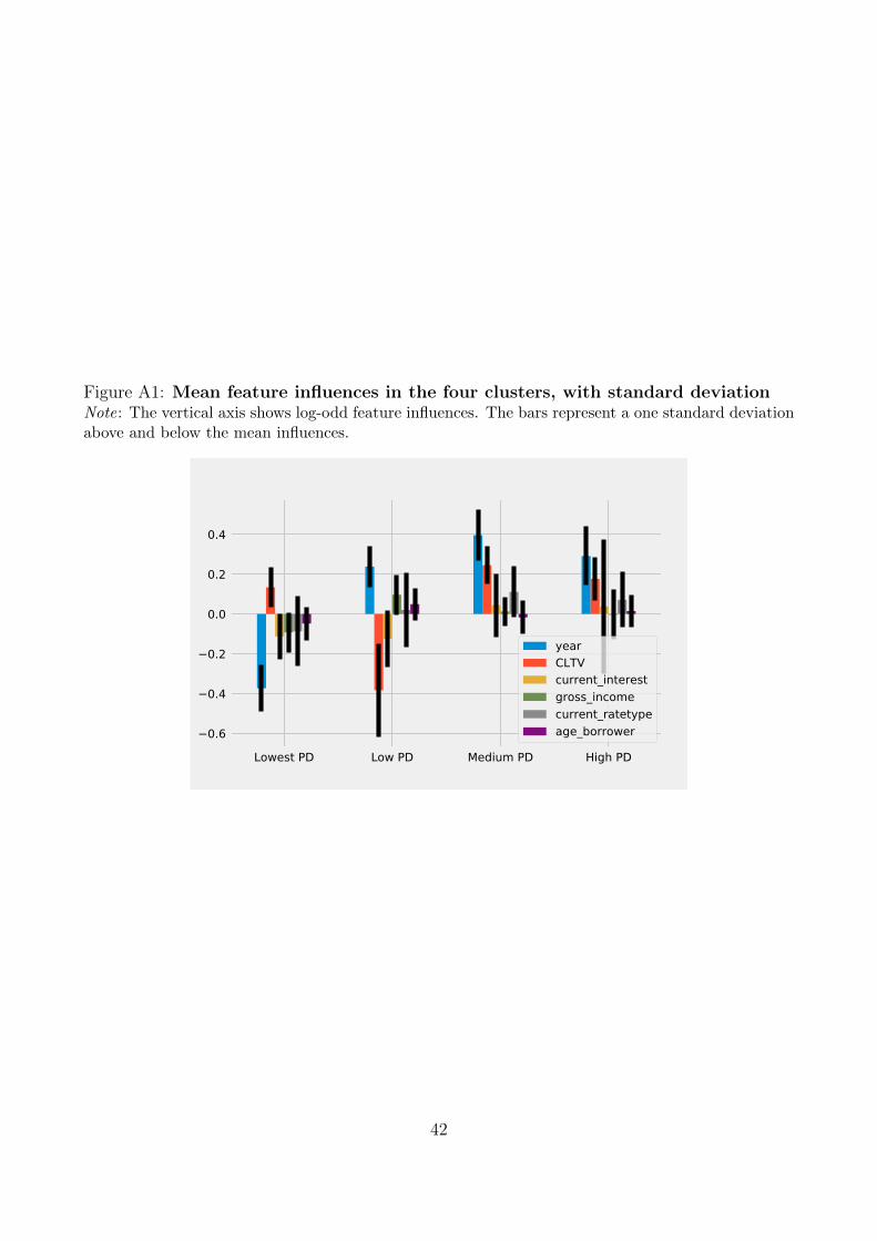
Figure A1: Mean feature influences in the four clusters, with standard deviationNote: The vertical axis shows log-odd feature influences. The bars represent a one standard deviationabove and below the mean influences.
Lowest PD Low PD Medium PD High PD0.6
0.4
0.2
0.0
0.2
0.4
yearCLTVcurrent_interestgross_incomecurrent_ratetypeage_borrower
42
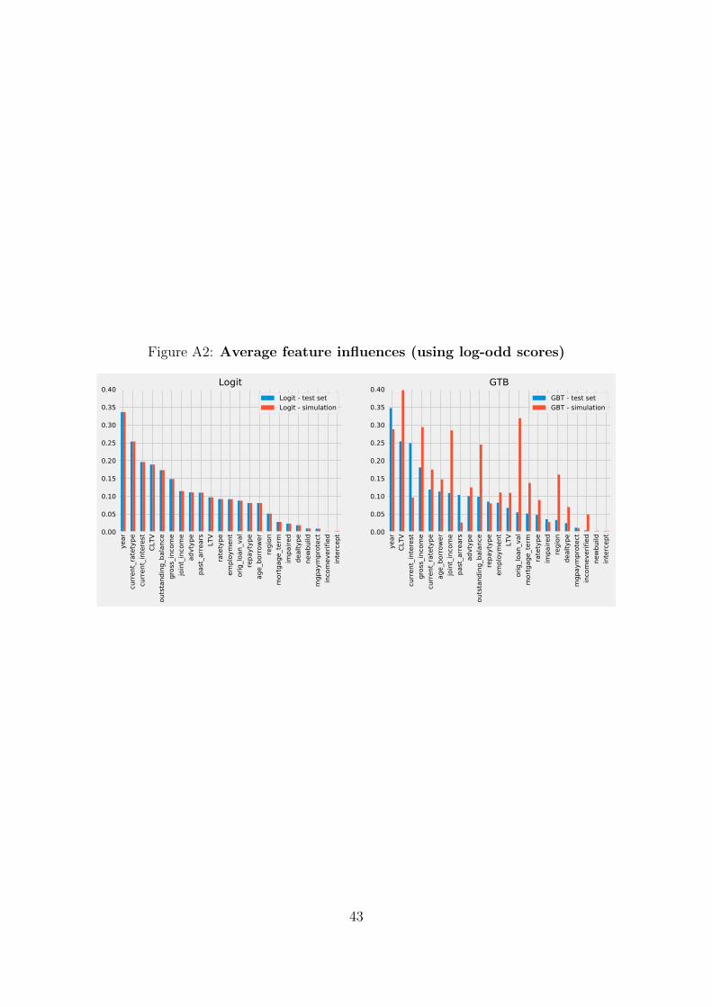
Figure A2: Average feature influences (using log-odd scores)
year
curre
nt_r
atet
ype
curre
nt_in
tere
stCL
TVou
tsta
ndin
g_ba
lanc
egr
oss_
inco
me
join
t_in
com
ead
vtyp
epa
st_a
rrear
sLT
Vra
tety
peem
ploy
men
tor
ig_lo
an_v
alre
payt
ype
age_
borro
wer
regi
onm
ortg
age_
term
impa
ired
deal
type
newb
uild
mgp
aym
prot
ect
inco
mev
erifi
edin
terc
ept0.00
0.05
0.10
0.15
0.20
0.25
0.30
0.35
0.40Logit
Logit - test setLogit - simulation
year
CLTV
curre
nt_in
tere
stgr
oss_
inco
me
curre
nt_r
atet
ype
age_
borro
wer
join
t_in
com
epa
st_a
rrear
sad
vtyp
eou
tsta
ndin
g_ba
lanc
ere
payt
ype
empl
oym
ent
LTV
orig
_loan
_val
mor
tgag
e_te
rmra
tety
peim
paire
dre
gion
deal
type
mgp
aym
prot
ect
inco
mev
erifi
edne
wbui
ldin
terc
ept0.00
0.05
0.10
0.15
0.20
0.25
0.30
0.35
0.40GTB
GBT - test setGBT - simulation
43