Banking the group: Impact of credit and linkagesamong Ugandan savings groups∗

Alfredo Burlando, Jessica Goldberg and Luciana Etcheverry †

January 3, 2020

Abstract

Traditional banks and microfinance institutions lend directly to clients using in-dividual or joint liability contracts, and generally have strict rules on selection andrepayments. In most rural areas of sub-Saharan Africa, these formal institutions areuncommon. Financial services are more often provided by savings groups; however,these are often unable to fully meet local financial needs. In this paper, we study analternative lending model with the potential to bridge the gap between formal andinformal finance. In this delegated lending model, better known as linkage, a formalfinancial institution lends to savings groups and lets the group decide the allocationof borrowed funds. In our RCT, a random sample of existing savings groups gainedaccess to linkage loans from a commercial bank in Uganda. We show that the bankloan stimulated an immediate and sizable increase in internal lending, which is sus-tained over time. Despite this benefit, we also find that linkages are a double-edgedsword: On the one hand, members of treated groups had temporarily lower rates offood insecurity after two years, and point estimates suggest sizable increases in incomeand microenterprise size (which are not statistically significant). On the other hand,groups assigned to loans experienced significantly more turnover, suggesting that thepossibility of external financing generates powerful selection effects.JEL classification: O12, O16Keywords: Savings groups, VSLA, Linkage, Financial inclusion, Microfinance, Mi-crolending, Selection.

∗Authors wish to thank Bjorn Stian Hellgren, Priscilla Mirembe Seruka, Alex Katende, Adrine Atusasire,Rita Larok, Amon Natukwatsa, Joshua Bwiira, Patrick Walugembe for their significant contributions in thefield. A special acknowledgement to Kristina Walker Nordlof, who started this project. Matt Steiger, MattDodier, Matt Summers, and Michael Enseki-Frank provided excellent RA and field assistance. Eliana laFerrara, Basile Grassi, Ketki Sheth, Paul Rippey, David Pannetta, Roy Mersland, seminar participants atEASST Summit, Bocconi University, University of Milano-Bicocca, and Agder University provided helpfulfeedback. We gratefully acknowledge the financial support of Strommestiftelsen, Fahu Foundation, and theSEEP Network.

†Burlando: University of Oregon, burlando@uoregon.edu. Goldberg: University of Maryland, gold-berg@umd.edu. Etcheverry: University of Oregon, lucianae@uoregon.edu.

1

1 Introduction

Credit is an important yet often missing element in the production process in low income

countries. Farmers need credit to make investments, confront a cyclical earnings cycle, and

smooth out unexpected income or consumption shocks. Microentrepreneurs also confront

cyclical demand and the need to make relatively large investments in stock or machinery.

Despite such needs, many rural communities are often underserved by financial institutions,

including microfinance. Traditional lending models, including microfinance, rely on individ-

ual or joint liability contracts which generally have strict rules on selection and repayments,

and are not very common in rural parts of sub-Saharan Africa.

In this study, we seek to better understand the impact of delegated credit, delivered by

a commercial bank to a savings group rather than an individual. Savings groups already

provide financial intermediation to millions of households in rural areas of sub-Saharan Africa

(Allen and Panetta, 2010, Karlan, Savonitto, Thuysbaert, and Udry, 2017), but remain

largely disconnected from formal credit markets. With delegated credit, which is better

known as “linkage credit”, the bank offers a loan with specific terms (interest rates and

repayment plans), and savings groups on-lend the external credit to members, using the

(generally more flexible) terms of credit that are prevalent in that group. Repayments to

the bank are generated through savings accumulation and repayment of internal loans, and

are not tied directly to those who (indirectly) borrowed from the bank.

To understand the impact of this novel type of finance, we randomly introduced a del-

egated credit product to existing savings groups in five districts in Uganda. Together with

a complementary savings account, loans are provided to the group as a whole, and not to

any single individual. In this paper, we show how credit linkage generates new internal

lending, and then report on the extent to which savings groups participants benefit from

delegated bank credit. The potential expansion of credit operates through a very specific

credit rationing channel: the bank provides additional funds to the group, and the group

2

uses those funds to provide credit to members. Note that groups already provided loans to

members; moreover, while the interest rate charged by the bank generally differs from the

interest rate charged internally by the group to its members, this internal rate is unaffected

by the additional funds. In other words, the product increases the quantity of credit, but

not its price.

In addition to the expansion of credit, the adoption of formal financial products is likely to

impact the groups through a number of other channels. First, the associated savings account

allows groups to store excess funds in a safe place, and thus reduce the need to over-lend at

the end of each cycle and the ability to lend money saved in the bank (if this is not easily

accessible to members). Second, the intervention provided a great deal of personal contact

with bank agents, thus improving the information available to members about the banking

system. We expect that this might generate spillovers from group accounts to individual

accounts. Finally, we expect that the program changes the incentives to join and remain in a

treated group. For instance, these groups may become more attractive to households seeking

larger loans, or less attractive to savers who face reductions in returns to their savings.

Our study, started in 2015, provided training and facilitated access to these formal finan-

cial products through 2016. Our data collection effort took place in February-March 2018,

less than two years after the intervention. By the end of the implementation period, two

thirds of the targeted groups had submitted a loan request, and one third had received a loan

from the bank. We find high rates of pass-through of the loan: internal loans to members are

four times higher in the week of the bank loan receipt relative to the expected amount; the

increase is around 1 million shillings, or 40% of the average first-time bank loan (2.3 million

shillings). We find that the internal loans generated are not larger in size; thus, the increase

in lending comes from an increase in the number of loans generated. Despite evidence that

internal lending amounts increased in a sustained way, a majority of groups stopped bor-

rowing from the bank after the initial loan allocation, suggesting that the benefits from the

3

program were not sufficient to overcome the costs of continued engagement.

In terms of welfare impacts, in the short run, the intervention raised financial resources

available to members, lowered rates of food insecurity; however, the relatively sizable increase

in household income does not raise to the level of statistical significance. Moreover, all ben-

efits wore off by the end of the study. On household production, we find fewer households

investing in agriculture, and statistically insignificant increases in enterprise sizes (as mea-

sured by revenues and costs) as well as profits. As for the other outcomes, point estimates

are larger at midline.

These moderate effects are modulated by the finding that groups exposed to the treat-

ment suffered from higher rates of member dropout. This is the result of increased churn

within groups, and not of increased group mortality. After three years, the gap in dropout

rates between treated and control groups is somewhat smaller and becomes statistically

insignificant, indicating some catching up by control groups.

The findings are consistent with the idea that linkage helps relax liquidity constraints

in the group, but the average benefit from linkage do not appear to be sufficiently high to

cover the significant recurrent costs. The muted impacts on investments are also consistent

with a broader literature that finds small average impacts from microfinance interventions

(Banerjee et al., 2015), which is puzzling given that investment returns appear to be high

in rural areas among credit borrowers (Beaman et al., 2014). The fact that external credit

generated changes in group membership is consistent with other experiments of delegated

credit (Maitra et al., 2017).

The rest of the paper is organized as follows. Section 2 provides information on financial

linkages, in Uganda and elsewhere; details on the accounts offered in our study; an expla-

nation of the structure of the intervention; a discussion of study timeline and instruments.

Section 3 discussed the estimation strategy adopted. Section 4 reports the results. Section

5 concludes.

4

2 Background information

2.1 Savings Groups

Savings groups are community-based financial institutions, whose members save on a weekly

basis, are able to accumulate those savings through a storage technology (typically, a sav-

ings box), and use those accumulated savings to generate interest bearing loans to members.

Thus, savings groups provide a degree of financial intermediation in the community. Consis-

tent with groups matching savers and borrowers, Cassidy and Fafchamps (2015) show that

there is negative assortative matching along time consistency. A number of impact evalu-

ation studies found that the introduction of savings groups improves food security, overall

consumption smoothing, livestock holding, household business outcomes and women’s em-

powerment(Ksoll, Lilleør, Lønborg, and Rasmussen, 2015, Beaman, Karlan, and Thuysbaert,

2014, Gash and Odell, 2013, Karlan, Savonitto, Thuysbaert, and Udry, 2017); however, these

welfare impacts are quite muted, raising the question of why the increase in financial inter-

mediation created by savings groups does not improve outcomes.

Savings groups are quickly becoming common in both rural and urban areas of Uganda

and elsewhere. According to the latest Finscope figures, almost half of households in Uganda

belong to one (FinScope, 2018).

2.2 Financial Linkage

Formal banking products that are targeted specifically to the savings group are called linkage

products. Banks may offer a group savings account, which can be used by the group to store

excess funds. Group savings account protect savings from theft or misuse; however, they also

raise the cost of accessing the group’s liquidity, as accessing the funds may involve time and

travel to a bank branch of mobile money operator. A second product, and the focus of this

paper, is a bank loan, offered to the group. The bank loan raises the liquidity of the group,

5

and allows more internal loans to be generated and issued. According to the State of linkage

report, as of 2016 25 banking institutions in 27 sub-Saharan countries offered some type

of linkage product to groups. In Uganda, where savings groups are particularly prevalent,

at the time of the intervention there were six different financial institutions offering these

products.

It is important to explain how these two products integrate with the daily operations of

the savings group. Savings account provide an alternative location to members’ funds. They

are safer than a lock-box, and thus should alleviate the fear of losing funds to theft. On

the other hand, because funds in savings accounts are less liquid, accounts may discourage

internal lending. The loan product increases the funds available to the group for internal

lending; note that the interest rate charged by the bank is lower than the rate charged

internally by the group (that rate varies from a minimum of 3% per month to 10% per

month), and that internal loans generated by the bank loan are priced at the internal rate.

2.3 The Opportunity Bank product

We study a linkage product offered by Opportunity Bank Uganda LTD. (OBUL) and mar-

keted around the country concurrently with the study. Bank loans range between one and

20 million UGX and carry a monthly interest of 2.75%. Repayment periods vary from three

to nine months. The initial loan was always limited to no more than five million UGX,

with a three month repayment period. Issued loans are given to the group and not to any

one individual, and are used to generate internal loans to members who borrow using the

internal rates. Groups repay the bank on a monthly basis, either via cash payments to a

bank representative, or through the mobile network or bank branch. Crucially, and unlike

more standard microfinance interventions, repayments to the bank are generated through

the cashflow of the group, i.e., from savings and internal loan repayments. These cash flows

need not coincide with the repayments issued by those members who borrowed from the

6

bank’s funds.

The process of linking the group to Opportunity Bank is not straightforward. First,

groups must be formally registered with local authorities (at the parish level). Usually, reg-

istration requires completing a registration form and obtaining signatures from community

representatives. Second, groups need to have a (free) group savings account, held at an OB

branch. The bank uses the account to manage loan deposit and payments, but groups can

also use it to store excess savings. Third, financial regulations require borrowing groups

to have financial identification cards, issued by the Government of Uganda. To meet these

regulations, three representatives of the group complete a financial card request under their

name; deposit a biometric reading of the fingers; and pay a one-time fee of UGX 15,000

(USD 5) each. These actions require a visit to the branch1. Fourth, groups complete a loan

application form, which include an extensive set of documents (see figure 3). Finally, branch

managers take two weeks or longer to decide whether to approve the loan request. Approved

loans are then deposited into the group’s group saving account, after a number of banking

fees and duties totaling UGX 120,000 (USD 35) have been subtracted from the loan.

As the above makes clear, while there are significant one-time learning and financial

costs involved in linkage, groups also face large recurring costs in maintaining these linkages.

Secondly, linked groups gain access to a savings product, in addition to the bank loan. Part

of the way groups respond to linkage may thus be mediated through the acquisition of this

savings account. To account for this, our intervention will attempt to separate the effect of

savings from those of credit.

1The creation of financial cards turned out to be very time consuming; biometric readers often failed torecognize all ten fingers, took hours to complete, and often were unsuccessful.

7

3 The intervention

Our intervention is registered under AEACTR-0003613 and took place in five districts of

Central Uganda: Buikwe, Luweero, Nakaseke, Nakasongola, and Wakiso. In each district,

we partnered with one of two local NGOs, READ Uganda and Project SCORE, to enroll

savings groups in the study and provide support to the research team. These NGOs were

chosen due to their focus on savings group formation, their active and ongoing support to

groups they formed, and their ability to intermediate between groups, research teams, and

representatives of the commercial bank.

Groups enrolled in the study were assigned to one of three treatment arms: a control

group, a “savings only” intervention, and a “savings + loan” intervention. Groups assigned

to one or both financial products received an intervention package that consisted in a number

of activities aimed at lowering the implicit and explicit costs of linking to the bank. Groups

received numerous visits from NGO and bank representatives, during which the group was

able to learn about the linkage process, the terms of the products, and the requirements

needed to successfully obtain a financial product. The study also facilitated the formal

registration of the savings group within local authorities, and helped filling out the applica-

tions for the savings accounts and loans. To further reduce transaction costs, the research

team paid the one-time fees associated with the financial cards. The overall intervention,

spread over a period of months, was very intensive, went beyond the standard engagement

of commercial banks, and was not cost effective.

One noteworthy difficulty in organizing this linkage product is that the bank branch

managing the intervention was located 60 to 100 km from study communities. To reduce

the substantial transaction costs associated with managing the savings and loan accounts,

group had the ability to administer some transactions remotely, through mobile money. In

addition, on occasion an OB mobile branch (located inside an armored truck) visited the

study communities to carry out banking transactions.

8

3.1 Study timeline

In late 2014 and early 2015, a research team representative visited approximately 300 VSLAs

in five Central Region districts served by READ Uganda and SCORE program in order to

screen groups based on their overall capacity and performance. The screening tool employed

was developed by CARE to help commercial banks identify groups that could benefit from

a formal bank linkages, and was considered state of the art at the time of the study. Groups

were enrolled in the study if they scored sufficiently high in the questionnaire, and were

thus considered to be highly likely to be acceptable for the commercial bank. In total, 156

groups were selected for the study, and randomized into the three treatment arms. To avoid

cross-treatment spillovers, treatment assignment was done at the level of the village.2

In February-April 2015, baseline interviews were carried out in all study groups. For

each group, 15 respondents were selected for the baseline. The intervention phase was slated

to begin immediately after randomization. However, a series of delays caused by the speed

of governmental approvals and commercialization of the product pushed the start date well

past the baseline and into early 2016. At that time, the commercial bank hired a field agent

solely devoted to marketing the product to savings groups in the study and helping the

groups navigate the linkage process.

The active intervention period lasted one year and ended in December 2016. After that

date, the bank field agent was relocated to a different branch and support activities to

study groups ended. To measure impacts, the research team collected midline surveys in

February-April of 2018, and the endline survey one year later, between February and April

of 2019.

It is important to highlight that the product became available in all OBUL branches at

2Because not all groups in a village participated in the study, villages assigned to the loan treatmentwill generally have groups where linkage did not take place. Groups in study villages might not have beenpart of the study for a variety of reasons, including: failure to score sufficiently high in the screening tools;not being supported by the SCORE or READ; refusal to participate in the study; refusal to being screened;were not in session at the time of the screening.

9

the start of our intervention in 2015, potentially leading to program spillovers. However, the

company introduced it in the areas under study in a controlled way, and was not allowed to

market other individual products to savings groups members during the intervention period.

Indeed, OB followed the protocol closely and there is no evidence of program spillovers in

our study areas.

3.2 Data

Data for the study comes from a variety of sources. Our main results originate from three

rounds of household surveys, carried out at baseline (in 2015), midline (in 2018) and endline

(2019); since the intervention took place in 2016, these surveys allow us to measure the

impacts of the intervention after two and three years. Surveys included primary outcomes of

interest: self reported amount of savings and loans, participation status with savings groups,

satisfaction with the group; household assets, earnings, and investments. The sample at

midline and endline included all those who were interviewed at baseline. At endline, we also

interviewed all other current members of the study groups. To create tracking sheets for this

exercise, between December 2018 and January 2019 a small team visited all groups and took

pictures of the current participant rosters. We then identified those that had not yet been

interviewed by their name. New interviewees thus consisted of long-time members (that is,

those who were members in 2015 but were not randomly selected for inclusion in the panel

sample) and newcomers, who joined the group at some point between 2016 and 2019.

In addition to the interview sample, our analysis incorporates information from a variety

of other sources. We received information on group loans offered in the study area from

Opportunity Bank; these include issuance and repayment dates plus loan amounts of all

loans to study groups for the year 2016 and 2017. In 2019 we also photographed and

digitized loan ledger books belonging to most (but not all) of the study groups. The loan

groups provide information on internal loans generated, including the issuance date and loan

10

amounts.

Summary statistics Table 1 provide summary statistics and balance tests from the panel

sample, comparing the loan group against the control. The top panel reports average re-

spondent characteristics at baseline. Two thirds of group participants are women, and the

average years of education is 2.8. As expected from the mostly rural location of the study,

approximately 70% of households are engaged in agriculture. Members are financially active

within VSLAs: 82% borrowed at least once in the previous cycle. However, as only 3% of

households reported having a loan from a formal lender, the sample is not accustomed to

working with the formal financial sector. Characteristics are well balanced between the two

treatment arms.

The bottom panel of the table reports summary statistics of the variables that appear in

the screening tool. Taken together, loan groups are similar control groups: key measures of

group performance –savings volumes, writeoffs, value of investments–are similar across the

two treatment arms. There is one variable that is unbalanced and that is portfolio at risk.

To account for any possible imbalance, we will control for all baseline variables in this table

in our regressions.

Table 2 reports the summary statistics of the sample of internal loans collected from

the group ledgers. We have information on 110 of the 145 groups; on average, each group

reported 140 loans over the period under consideration. Loan Amounts indicates the average

value of a loan, which is UGX 350,000.

4 The provision of credit within the savings group

In this section, we describe the take-up of the bank loan by treated groups, and then show

the extent to which the additional funds are on-lent to the membership.

11

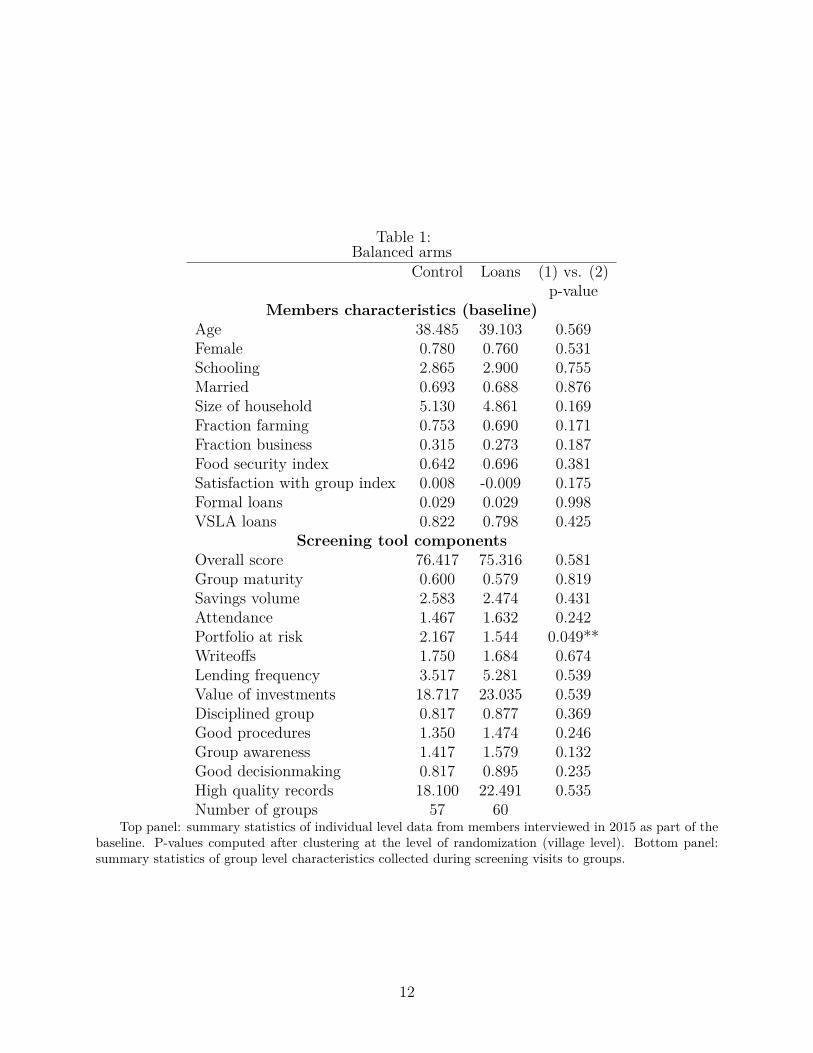
Table 1:Balanced arms

Control Loans (1) vs. (2)p-value

Members characteristics (baseline)Age 38.485 39.103 0.569Female 0.780 0.760 0.531Schooling 2.865 2.900 0.755Married 0.693 0.688 0.876Size of household 5.130 4.861 0.169Fraction farming 0.753 0.690 0.171Fraction business 0.315 0.273 0.187Food security index 0.642 0.696 0.381Satisfaction with group index 0.008 -0.009 0.175Formal loans 0.029 0.029 0.998VSLA loans 0.822 0.798 0.425

Screening tool componentsOverall score 76.417 75.316 0.581Group maturity 0.600 0.579 0.819Savings volume 2.583 2.474 0.431Attendance 1.467 1.632 0.242Portfolio at risk 2.167 1.544 0.049**Writeoffs 1.750 1.684 0.674Lending frequency 3.517 5.281 0.539Value of investments 18.717 23.035 0.539Disciplined group 0.817 0.877 0.369Good procedures 1.350 1.474 0.246Group awareness 1.417 1.579 0.132Good decisionmaking 0.817 0.895 0.235High quality records 18.100 22.491 0.535Number of groups 57 60

Top panel: summary statistics of individual level data from members interviewed in 2015 as part of thebaseline. P-values computed after clustering at the level of randomization (village level). Bottom panel:summary statistics of group level characteristics collected during screening visits to groups.

12

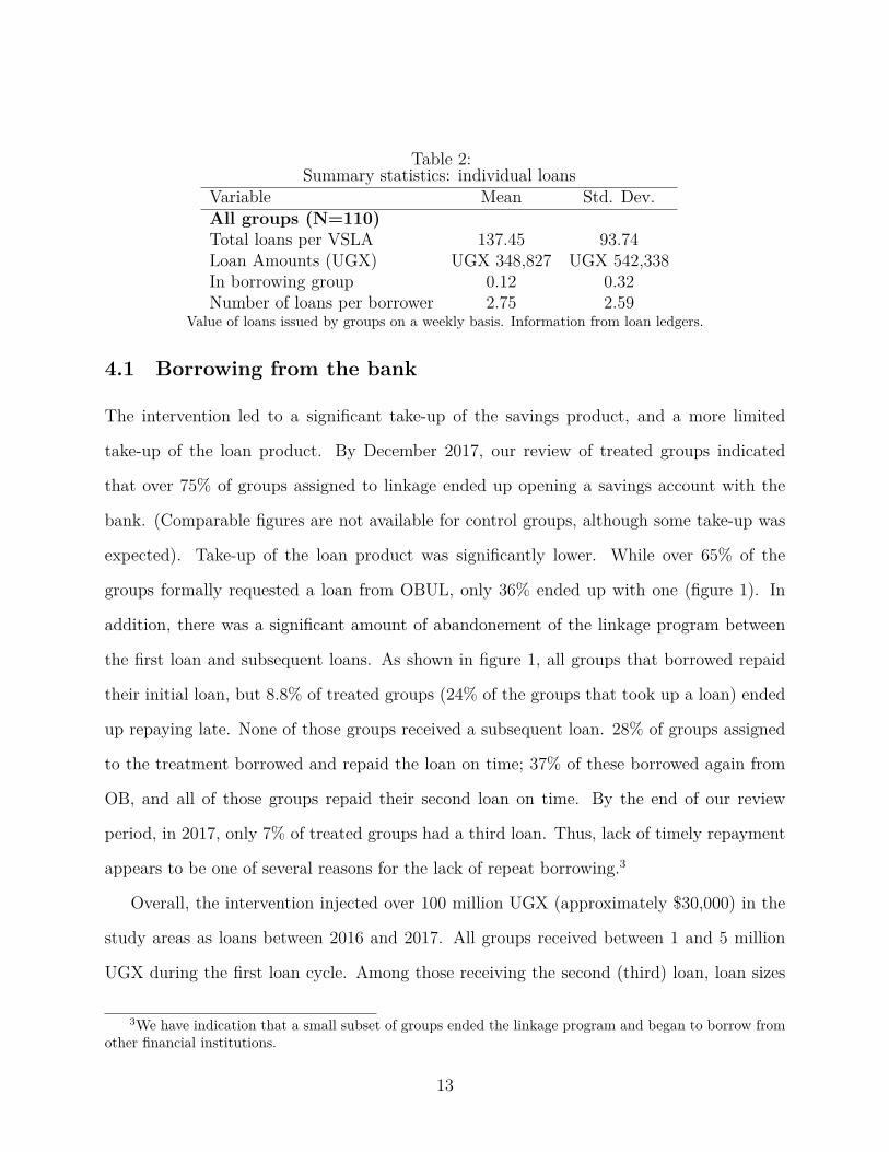
Table 2:Summary statistics: individual loans

Variable Mean Std. Dev.All groups (N=110)Total loans per VSLA 137.45 93.74Loan Amounts (UGX) UGX 348,827 UGX 542,338In borrowing group 0.12 0.32Number of loans per borrower 2.75 2.59

Value of loans issued by groups on a weekly basis. Information from loan ledgers.

4.1 Borrowing from the bank

The intervention led to a significant take-up of the savings product, and a more limited

take-up of the loan product. By December 2017, our review of treated groups indicated

that over 75% of groups assigned to linkage ended up opening a savings account with the

bank. (Comparable figures are not available for control groups, although some take-up was

expected). Take-up of the loan product was significantly lower. While over 65% of the

groups formally requested a loan from OBUL, only 36% ended up with one (figure 1). In

addition, there was a significant amount of abandonement of the linkage program between

the first loan and subsequent loans. As shown in figure 1, all groups that borrowed repaid

their initial loan, but 8.8% of treated groups (24% of the groups that took up a loan) ended

up repaying late. None of those groups received a subsequent loan. 28% of groups assigned

to the treatment borrowed and repaid the loan on time; 37% of these borrowed again from

OB, and all of those groups repaid their second loan on time. By the end of our review

period, in 2017, only 7% of treated groups had a third loan. Thus, lack of timely repayment

appears to be one of several reasons for the lack of repeat borrowing.3

Overall, the intervention injected over 100 million UGX (approximately $30,000) in the

study areas as loans between 2016 and 2017. All groups received between 1 and 5 million

UGX during the first loan cycle. Among those receiving the second (third) loan, loan sizes

3We have indication that a small subset of groups ended the linkage program and began to borrow fromother financial institutions.

13

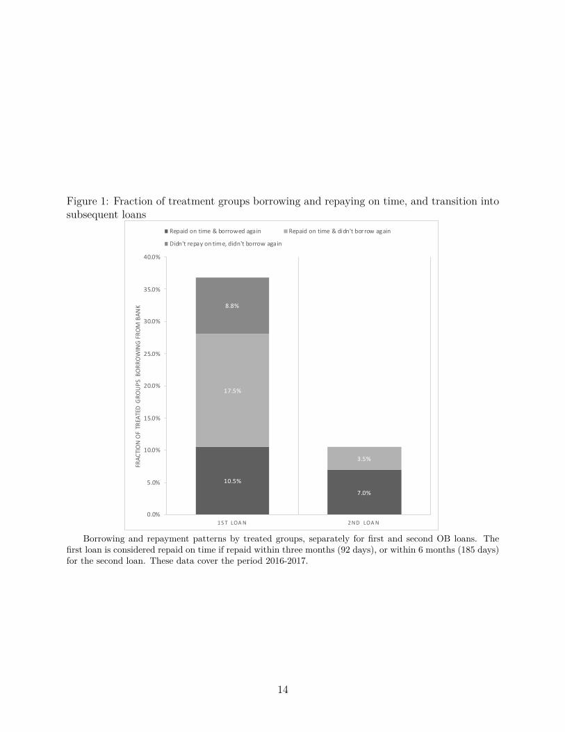
Figure 1: Fraction of treatment groups borrowing and repaying on time, and transition intosubsequent loans

17.5%

3.5%

10.5%

7.0%

8.8%

0.0%

5.0%

10.0%

15.0%

20.0%

25.0%

30.0%

35.0%

40.0%

1 S T LOA N 2 ND LOA N

FRAC

TIO

N O

F TR

EATE

D G

ROU

PS B

ORR

OW

ING

FRO

M B

ANK

Repaid on time & borrowed again Repaid on time & didn't borrow again

Didn't repay on time, didn't borrow again

Borrowing and repayment patterns by treated groups, separately for first and second OB loans. Thefirst loan is considered repaid on time if repaid within three months (92 days), or within 6 months (185 days)for the second loan. These data cover the period 2016-2017.

14

varied from 3 to 5 million (5 to 10 million) UGX.

4.2 Impact on internal lending

We next study the extent to which the external loan generated internal loans. To do so, we

adopt a leads-lags model of the following form:

LoanAmtit =20∑

j=−20

αjGroupLoang ×Weekjgt + δt + δg + εit, (1)

where LoanAmountsgt is the total value of internal loans given out in group g during

meeting week t; GroupLoang identifies groups that received the loan from Opportunity Bank;

Weekjgt is an indicator for week t for group g, which occurred j weeks before or after the

provision of the bank loan. The parameters are αj, which identify deviations of internal

lending from the expected amount j weeks before/after the receipt of the bank loan. To

control for seasonality and group characteristics, the regression includes VSLA fixed effects

and week-year fixed effects; the estimation of parameters αj arises from the variation in the

timing of the receipt of the bank loan. Identification assumes that the timing of receipt is

random, and independent of internal loan demand shocks. This is quite reasonable, as the

actual delivery of the bank loan depended on when (busy) loan officers gave final approval,

and were thus not timed to internal needs. Moreover, if groups did expect the bank loan to

arrive, then we should see αj ̸= 0 for j < 0.

Figure 2 plots the coefficient estimates αj for the forty week period surrounding the

issuance of the bank loan. We can see that the amounts lent increase substantially the

week the group receives the funds from the bank. The point estimate is close to one million

shillings, which is four times as high as the average amount lent (UGX 230,000) and is

40% of the UGX 2.3 million that linked groups received from the bank. The figure also

shows that the amounts do not increase substantially in the periods following the bank

15

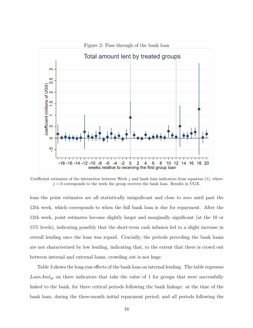
Figure 2: Pass through of the bank loan

Coefficient estimates of the interaction between Week j and bank loan indicators from equation (1), wherej = 0 corresponds to the week the group receives the bank loan. Results in UGX.

loan–the point estimates are all statistically insignificant and close to zero until past the

12th week, which corresponds to when the full bank loan is due for repayment. After the

12th week, point estimates become slightly larger and marginally significant (at the 10 or

15% levels), indicating possibly that the short-term cash infusion led to a slight increase in

overall lending once the loan was repaid. Crucially, the periods preceding the bank loans

are not characterized by low lending, indicating that, to the extent that there is crowd out

between internal and external loans, crowding out is not huge.

Table 3 shows the long-run effects of the bank loan on internal lending. The table regresses

LoanAmtgt on three indicators that take the value of 1 for groups that were successfully

linked to the bank, for three critical periods following the bank linkage: at the time of the

bank loan; during the three-month initial repayment period; and all periods following the

16

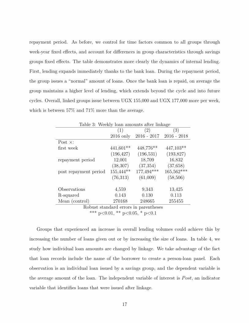
repayment period. As before, we control for time factors common to all groups through

week-year fixed effects, and account for differences in group characteristics through savings

groups fixed effects. The table demonstrates more clearly the dynamics of internal lending.

First, lending expands immediately thanks to the bank loan. During the repayment period,

the group issues a “normal” amount of loans. Once the bank loan is repaid, on average the

group maintains a higher level of lending, which extends beyond the cycle and into future

cycles. Overall, linked groups issue between UGX 155,000 and UGX 177,000 more per week,

which is between 57% and 71% more than the average.

Table 3: Weekly loan amounts after linkage(1) (2) (3)

2016 only 2016 - 2017 2016 - 2018Post ×:first week 441,601** 448,776** 447,103**

(196,427) (196,531) (193,827)repayment period 12,001 18,709 16,832

(38,307) (37,354) (37,658)post repayment period 155,444** 177,494*** 165,562***

(76,313) (61,009) (58,506)

Observations 4,559 9,343 13,425R-squared 0.143 0.130 0.113Mean (control) 270168 248665 255455

Robust standard errors in parentheses*** p<0.01, ** p<0.05, * p<0.1

Groups that experienced an increase in overall lending volumes could achieve this by

increasing the number of loans given out or by increasing the size of loans. In table 4, we

study how individual loan amounts are changed by linkage. We take advantage of the fact

that loan records include the name of the borrower to create a person-loan panel. Each

observation is an individual loan issued by a savings group, and the dependent variable is

the average amount of the loan. The independent variable of interest is Post, an indicator

variable that identifies loans that were issued after linkage.

17

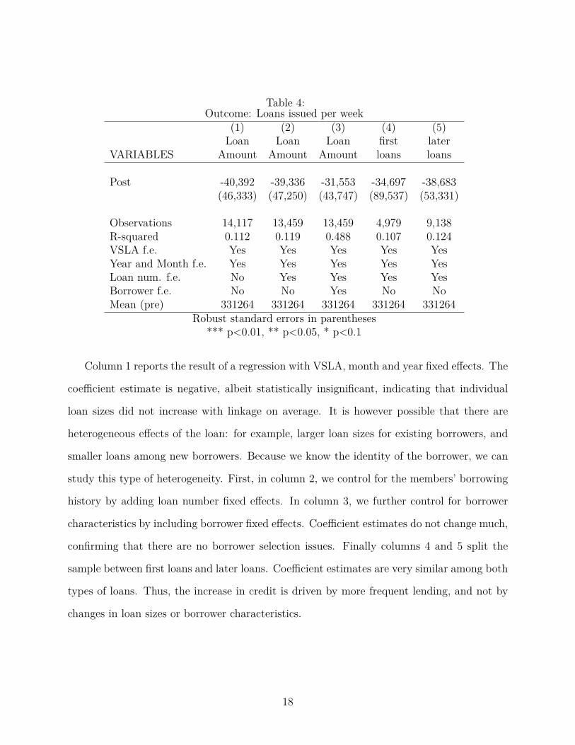
Table 4:Outcome: Loans issued per week

(1) (2) (3) (4) (5)Loan Loan Loan first later

VARIABLES Amount Amount Amount loans loans

Post -40,392 -39,336 -31,553 -34,697 -38,683(46,333) (47,250) (43,747) (89,537) (53,331)

Observations 14,117 13,459 13,459 4,979 9,138R-squared 0.112 0.119 0.488 0.107 0.124VSLA f.e. Yes Yes Yes Yes YesYear and Month f.e. Yes Yes Yes Yes YesLoan num. f.e. No Yes Yes Yes YesBorrower f.e. No No Yes No NoMean (pre) 331264 331264 331264 331264 331264

Robust standard errors in parentheses*** p<0.01, ** p<0.05, * p<0.1

Column 1 reports the result of a regression with VSLA, month and year fixed effects. The

coefficient estimate is negative, albeit statistically insignificant, indicating that individual

loan sizes did not increase with linkage on average. It is however possible that there are

heterogeneous effects of the loan: for example, larger loan sizes for existing borrowers, and

smaller loans among new borrowers. Because we know the identity of the borrower, we can

study this type of heterogeneity. First, in column 2, we control for the members’ borrowing

history by adding loan number fixed effects. In column 3, we further control for borrower

characteristics by including borrower fixed effects. Coefficient estimates do not change much,

confirming that there are no borrower selection issues. Finally columns 4 and 5 split the

sample between first loans and later loans. Coefficient estimates are very similar among both

types of loans. Thus, the increase in credit is driven by more frequent lending, and not by

changes in loan sizes or borrower characteristics.

18

5 Impact of linkage on members

In the previous section, we demonstrated that linkage changed the borrowing patterns within

linked savings groups. We next use household level surveys carried out in 2018 and 2019 to

study whether exposure to the linkage program impacted living standards of members. In

our analysis, we take advantage of the panel feature of our data to use an intent-to-treat

methodology that controls for baseline characteristics. For each primary outcome, we run

the following regression at the individual i in village v:

yiv = α0 + α1Linked_Loanv +Xivβ + ϵiv. (2)

The independent variable of interest is Loanv, which is an indicator for household who

participated in groups located in villages v that were assigned to the loan intervention. All

specifications include five district fixed effects and Xig, a matrix of group and all household

and randomization controls reported in table 1. We also include the full set of employment

sector indicators (not reported in the table).

We run regression (2) on the midline and endline data separately, using the panel sample.

The estimated α1 will tell us the effect of assignment to a linkage program on those who

were targeted by the program.

To account for the fact that outcomes can be correlated at the group and village level, we

report standard errors that are clustered at the village level. In addition, we control for the

false discovery rate using the methods developed by Benjamini and Hochberg (1995). Since

the correction leads to more conservative confidence intervals, we report q-values only for

coefficients that are statistically significant without correction. We also report ITT results

for the midline (after two years) in panel A of each table, and for the endline (after three

years) in panel B. Discussion of panel C is left to section 6.

19

Household savings and credit We begin with the effect of the intervention on savings,

credit, and some measure of credit rationing. Table 6 reports results of regression (2),

where the dependent variable is the amount saved in formal savings accounts and VSLAs

(column 1), amount borrowed across available sources icluding VSLAs, banks, MFIs and

moneylenders, (column 2), and whether the person reported having had a loan denied by

a formal lender (column 3). Due to a coding error in our data collection tool at midline,

the questionnaire did not include savings and borrowing from all VSLAs, and thus the total

savings and credit amounts are available for the endline only. Point estimates for savings are

positive but insignificant, while for loans estimates are also positive (133,000 UGX, or slightly

less than $40) (p-value 0.151). Table 7 disaggregates saving by type (VSLA vs. formal);

estimates on savings continue to be statistically insignificant. Table 8 disaggregates credit

by lender type. We see that VSLA credit is larger in groups assigned to the loan linkage, by

approximately 144,000 UGX (18% of the average borrowed amount in the control group).

Estimates from the other sources are statistically insignificant. 4 We also find no evidence

that the intervention increased the likelihood of having a savings or loan account (results not

shown). Overall, these results clearly show that there are no effects of linkage on external

financial utilization. Finally, shareout amounts were somewhat higher in the treated group

(table 9). This is broadly consistent with higher internal fund utilization rate, derived from

increased in credit without a change in savings observed in treated groups. However, the

estimates fails to achieve statistical significance.

Impacts on income, investments, and business outcomes We next analyze the im-

pacts on income (table 10), use and amounts of agricultural inputs (table 11), and microen-

terprise outcomes (table 12). All results are noisy, and lack statistical significance; point

estimates are indicative of an increase in income, and a shift away from agricultural in-4It should be noted that the proportion of participants obtaining a loan from external sources is very

low–only 12% of the control sample did so, and only 2.6% obtained it from a bank. ITT coefficient estimatesare likewise very small, and largely statistically insignificant.

20

vestments towards microenterprise. At midline, point estimates for income indicate that

members assigned to the treatment had 15% higher income (p-value: 0.19), but these point

estimates fall and become even noisier at endline. On agricultural production, (table 11),

there is a significant reduction in the likelihood of use of agricultural inputs at endline (col-

umn 2), with the effect being driven by nonlabor inputs. However, this result does not

survive the FDR correction, and the average amount spent on inputs remains unchanged

across the treatment arms. Finally, table 12 measures treatment effects on enterprise devel-

opment. It should first be noted that all outcomes in the table are measured with significant

noise between one data collection round and the next, possibly indicating a high amount

of reporting bias. It is thus perhaps unsurprising that none of the outcomes measured are

statistically significant. The likelihood of having an enterprise is 1 p.p higher in the treated

group. When looking at those firms with an enterprise, we see positive point estimates for

profits (both computed and self reported), costs, and revenues at midline. However, all es-

timates are very noisy; moreover, the sample size is very small. At endline, point estimates

for costs remain as large as the midline, while revenues remain much smaller. Computed

profits are thus negative (albeit statistically insignificant). On the other hand, self-reported

profits remain positive and are close to significance (p-val 0.13).

Impacts on food security Table 13 analyzes the effect of the intervention on food inse-

curity. Food insecurity is measured from five questions, in increasing order of severity. At

midline, participants in treated groups report significantly fewer instances of food insecurity,

for all issues bar the most severe type. In total, they report 0.25 fewer issues (column 6),

i.e., 24% less than the control group. By endline, these differences had shrunk to zero. In

particular, the incidence of less severe issues (issues 1 and 2) in the control group do not

seem to change much between the two rounds of data collection, while the incidence for

the treated group does increase after the first year. The gains from the intervention are

21

short-lived.

Participation and satisfaction with the group We finally analyze the effect of the

intervention on members’ experiences with the group. First, we analyze whether the inter-

ventions caused differential attrition from the group. A priori, the effect of the treatment

is ambiguous. On the one hand, improved access to safe storage of funds and credit should

reduce attrition (at least among borrowers). On the other hand, external credit may reduce

savings returns, which is detrimental for savers. More generally, the decision to participate in

a linkage program can be controversial, given the low levels of trust in financial institutions

by Ugandans. If the program creates more discontent, we would expect to see an increase

in attrition.

Table 14 reports the result of a regression whose dependent variable is whether the

member reported not being a participant of the group. The loan treatment is strongly

associated with an increase in the likelihood of dropping out at midline: the estimate in

column 2 suggests a 8.4 percentage point increase over the control group (19.3%): this

represents an increase of 44% over the control mean. The coefficient estimate for the savings

only treatment is also positive and large in magnitude, but is not statistically significant. One

year later, more group participants had left both treated and control groups; the proportion

leaving was slightly higher in the control group, and the differences between the two are

no longer statistically significant. Nonetheless, the 6.2 p.p. difference is 24% of the control

mean, which is large. Thus, the intervention changed the composition of the group, but like

much else these changes fade over time.5

To shed some light on this result, table 15 regresses a “group satisfaction index” variable

on our ITT regressions for the midline. On average, study participants associated with the

loan intervention report lower (by 0.1 standard deviations) levels of satisfaction relative to

5It should be noted that this result is not driven by group mortality: none of the groups in the treatmentdismantled (and only two did in the control group).

22

control. Importantly, this lower satisfaction comes entirely from the dropouts (column 3),

while stayers’s satisfaction is unaffected by treatment. While it is not possible to glean the

causal chain here, the result is suggestive that the intervention did lead to reductions in

overall satisfaction and exit from the group.

6 Impact of linkage on the characteristics of the group

The discussion above indicates that exposure to linkage programs has muted welfare impacts,

but does cause an increase in turnover within savings groups. If the new members who replace

the leavers have characteristics that are very different from those leavers, they could change

the average characteristics of the group. On average, groups that have undergone linkage

could thus appear to be different; it would however be incorrect to attribute the difference as

a causal effect of linkage of members. The potential for misattribution of impacts on linkage

is quite possible: anecdotes of groups improving after linkage abound among the savings

group community.

To better understand the effect of linkage on the average characteristics of the group,

we make use of the full endline sample. As mentioned in the data section, at endline we

interviewed all members that were active in 2018, irrespective of whether they joined prior

or after the intervention. We then used these data to reconstruct all the (study) groups that

a household belonged to at endline, and created a dataset of household-by-group. For each

household i belonging to group g, we run the following regressions:

yig = α0 + α1Linked_Loang +Xigβ + ϵig. (3)

Note that equation (3) differs from (2) in a number of ways. First, the regression above

allows for multiple observations for each household, if households belong to multiple groups.

Second, the assignment to the treatment, Linked_Loan, is defined over the group that

23

household i belongs to, and not her village. For members that were present at baseline, we

thus ignore their initial assignment, and drop baseline observations that are no longer in a

study savings group in 2018. The estimated coefficient α1 thus indicates the difference in

outcome y between groups assigned to the linkage and control. The difference is a weighted

sum of two factors: the impact of linkage on stayers, and of the difference in the charac-

teristics of newcomers. Given that the first factor is estimated to be close to zero for most

outcomes, the coefficient estimate thus indicates the effect of selection.

We revisit all outcomes reported in section 5. For simplicity, estimates for equation (3)

are reported in panel C of each table presented in the previous section.

The results indicate that linkage does make groups appear better off–due to the selection

effects. Members of linked groups have higher savings and total loan amounts (table 6),

and gain from higher shareout amounts (table 9). On the other hand, it terms of measured

outcomes, coefficient estimates do not appear to be significantly larger in treated groups

relative to control. Income is higher (table 10) and standard errors are somewhat lower

although results remain insignificant; the patterns for agricultural production is also similar

to the endline panel sample. On enterprise, coefficients for self reported and imputed profits

are both positive and relatively small. Rates of food insecurity are also indistinguishable

between treated and control groups.

7 Conclusion

In this study, we seek to better understand the impact of credit delivered through savings

groups. Our randomized control trial enhances financial intermediation by introducing two

formal banking products–a savings account and a loan account– to existing savings groups

in five districts in Uganda. he main question we are interested in addressing is whether

savings groups participants benefit from an enhanced access to bank credit. The potential

24

expansion of credit operates through a very specific credit rationing channel: the bank pro-

vides additional funds to the group, and the group uses those funds to provide credit to

members. After two years, we find that most (75%) treated groups opened the account with

the banking institution. Take-up of loans was considerably lower: only one third of groups

were able to successfully receive a loan from the bank. Despite this, we observe a large

increase of lending to members coinciding with the bank loans, suggesting that the loan did

generate new borrowing opportunities. Our (preliminary and noisy) estimates suggest an

increase of 13% in self-reported income, and 17% increase in savings. We find some limited

spillover effects on personal use of loans from SACCOs, but these are limited to the savings

only intervention arm. Finally, we find no effects on agricultural investments (we have yet to

analyze impacts on enterprise). We also find that groups exposed to the treatment suffered

from higher rates of member dropout, which we aim to explain in greater detail in future

versions of the paper.

References

Allen, H. and D. Panetta (2010). Savings groups: What are they. SEEP Network.

Banerjee, A., D. Karlan, and J. Zinman (2015). Six randomized evaluations of microcredit:

Introduction and further steps. American Economic Journal: Applied Economics 7(1),

1–21.

Beaman, L., D. Karlan, and B. Thuysbaert (2014). Saving for a (not so) rainy day: A

randomized evaluation of savings groups in Mali. Technical report, National Bureau of

Economic Research.

Beaman, L., D. Karlan, B. Thuysbaert, and C. Udry (2014). Self-selection into credit mar-

25

kets: Evidence from agriculture in mali. Technical report, National Bureau of Economic

Research.

Benjamini, Y. and Y. Hochberg (1995). Controlling the false discovery rate: a practical and

powerful approach to multiple testing. Journal of the Royal statistical society: series B

(Methodological) 57(1), 289–300.

Burlando, A. and A. Canidio (2017). Does group inclusion hurt financial inclusion? ev-

idence from ultra-poor members of ugandan savings groups. Journal of Development

Economics 128, 24–48.

Cassidy, R. and M. Fafchamps (2015). Can community-based microfinance groups match

savers with borrowers? evidence from rural Malawi. working paper.

FinScope (2018). Topline findings report.

Gash, M. and K. Odell (2013). The evidence-based story of savings groups: A synthesis of

seven randomized control trials. SEEP Network.

Karlan, D., B. Savonitto, B. Thuysbaert, and C. Udry (2017). Impact of savings groups on

the lives of the poor. Proceedings of the National Academy of Sciences 114(12), 3079–3084.

Ksoll, C., H. B. Lilleør, J. H. Lønborg, and O. D. Rasmussen (2015). Impact of village savings

and loans associations: evidence from a cluster randomized trial. Journal of Development

Economics 120, 70 – 85.

Maitra, P., S. Mitra, D. Mookherjee, A. Motta, and S. Visaria (2017). Financing smallholder

agriculture: An experiment with agent-intermediated microloans in india. Journal of

Development Economics 127, 306–337.

26

8 Figures and Tables

Figure 3: OB loan application checklist

VSLA PRE-DISBURSMENT CHECKLIST

1 Fully filled and signed VSLA application form. 2 Committee approval. 3 VSLA rating for linkage/Assessment form. 4 VSLA decision making matrix 5 VSLA rating report 6 CRB search for the VSLA and the signatories. 7 Mandatory saving(20%) of loan approved 8 VSLA resolution to borrow 9 Identification and passports for the VSLA signatories. 10 Fully filled ID form for all the signatories. 11 L.C letter of recommendation to borrow for the VLSA. 12 Copy of certified VSLA registration certificate. 13 Copy of certified VSAL constitution. 14 Sketch map to the VSLA sitting venue. 15 Group photo 16 Have all the committee recommendations been full filled?

RO NAMES: _____________________ Branch Manager: Branch Operations Manager

Signature: ______________________ ___________________ ____________________

Date:____________________ ___________________ ____________________

27

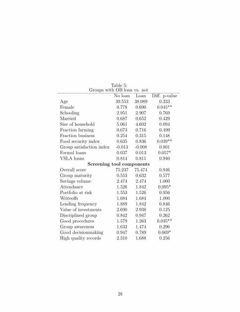
Table 5:Groups with OB loan vs. not

No loan Loan Diff. p-valueAge 39.553 38.089 0.333Female 0.778 0.690 0.045**Schooling 2.951 2.907 0.769Married 0.687 0.652 0.429Size of household 5.061 4.602 0.094Fraction farming 0.673 0.716 0.499Fraction business 0.254 0.315 0.148Food security index 0.635 0.836 0.039**Group satisfaction index -0.013 -0.008 0.801Formal loans 0.037 0.013 0.057*VSLA loans 0.814 0.811 0.940

Screening tool componentsOverall score 75.237 75.474 0.946Group maturity 0.553 0.632 0.577Savings volume 2.474 2.474 1.000Attendance 1.526 1.842 0.095*Portfolio at risk 1.553 1.526 0.956Writeoffs 1.684 1.684 1.000Lending frequency 1.889 1.842 0.846Value of investments 2.690 2.938 0.125Discriplined group 0.842 0.947 0.262Good procedures 1.579 1.263 0.035**Group awareness 1.632 1.474 0.296Good decisionmaking 0.947 0.789 0.069*High quality records 2.310 1.688 0.256

28

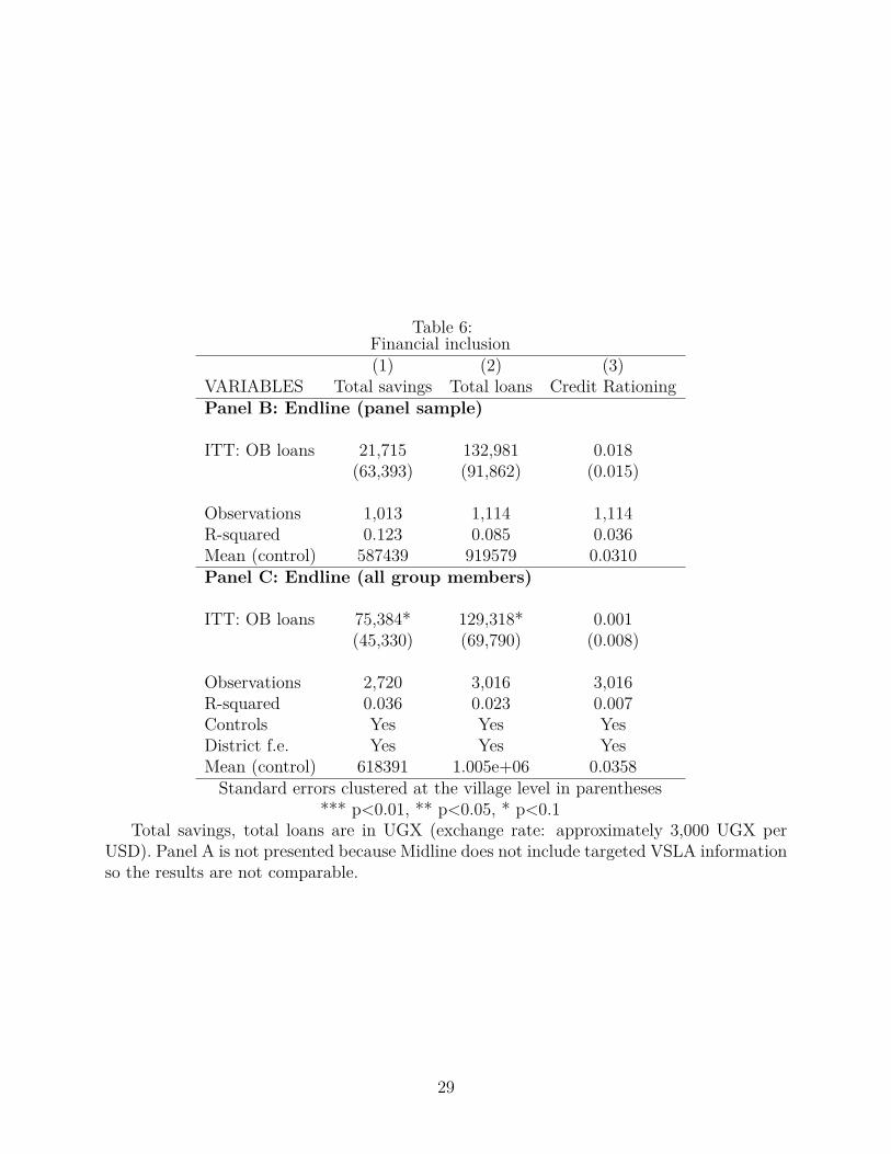
Table 6:Financial inclusion(1) (2) (3)

VARIABLES Total savings Total loans Credit RationingPanel B: Endline (panel sample)

ITT: OB loans 21,715 132,981 0.018(63,393) (91,862) (0.015)

Observations 1,013 1,114 1,114R-squared 0.123 0.085 0.036Mean (control) 587439 919579 0.0310Panel C: Endline (all group members)

ITT: OB loans 75,384* 129,318* 0.001(45,330) (69,790) (0.008)

Observations 2,720 3,016 3,016R-squared 0.036 0.023 0.007Controls Yes Yes YesDistrict f.e. Yes Yes YesMean (control) 618391 1.005e+06 0.0358Standard errors clustered at the village level in parentheses

*** p<0.01, ** p<0.05, * p<0.1Total savings, total loans are in UGX (exchange rate: approximately 3,000 UGX per

USD). Panel A is not presented because Midline does not include targeted VSLA informationso the results are not comparable.

29

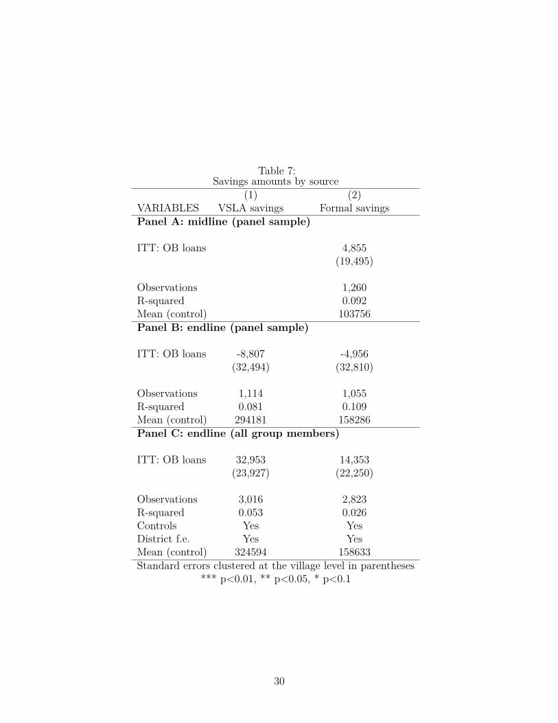
Table 7:Savings amounts by source

(1) (2)VARIABLES VSLA savings Formal savingsPanel A: midline (panel sample)

ITT: OB loans 4,855(19,495)

Observations 1,260R-squared 0.092Mean (control) 103756Panel B: endline (panel sample)

ITT: OB loans -8,807 -4,956(32,494) (32,810)

Observations 1,114 1,055R-squared 0.081 0.109Mean (control) 294181 158286Panel C: endline (all group members)

ITT: OB loans 32,953 14,353(23,927) (22,250)

Observations 3,016 2,823R-squared 0.053 0.026Controls Yes YesDistrict f.e. Yes YesMean (control) 324594 158633Standard errors clustered at the village level in parentheses

*** p<0.01, ** p<0.05, * p<0.1

30

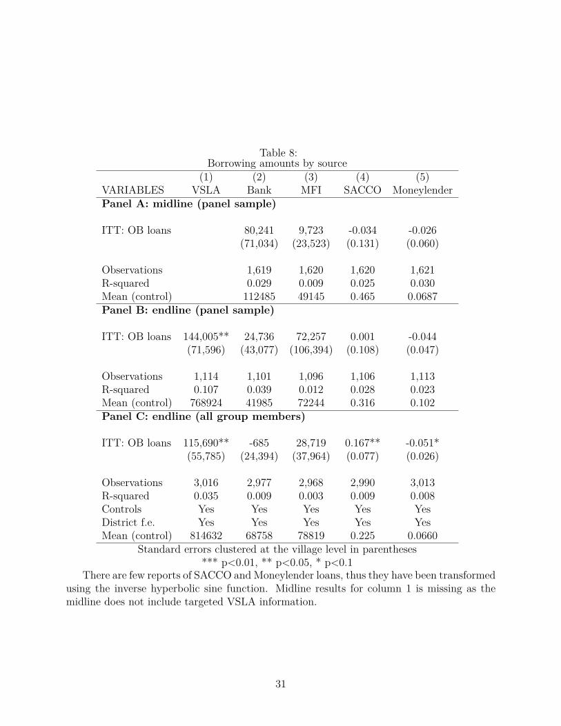
Table 8:Borrowing amounts by source

(1) (2) (3) (4) (5)VARIABLES VSLA Bank MFI SACCO MoneylenderPanel A: midline (panel sample)

ITT: OB loans 80,241 9,723 -0.034 -0.026(71,034) (23,523) (0.131) (0.060)

Observations 1,619 1,620 1,620 1,621R-squared 0.029 0.009 0.025 0.030Mean (control) 112485 49145 0.465 0.0687Panel B: endline (panel sample)

ITT: OB loans 144,005** 24,736 72,257 0.001 -0.044(71,596) (43,077) (106,394) (0.108) (0.047)

Observations 1,114 1,101 1,096 1,106 1,113R-squared 0.107 0.039 0.012 0.028 0.023Mean (control) 768924 41985 72244 0.316 0.102Panel C: endline (all group members)

ITT: OB loans 115,690** -685 28,719 0.167** -0.051*(55,785) (24,394) (37,964) (0.077) (0.026)

Observations 3,016 2,977 2,968 2,990 3,013R-squared 0.035 0.009 0.003 0.009 0.008Controls Yes Yes Yes Yes YesDistrict f.e. Yes Yes Yes Yes YesMean (control) 814632 68758 78819 0.225 0.0660

Standard errors clustered at the village level in parentheses*** p<0.01, ** p<0.05, * p<0.1

There are few reports of SACCO and Moneylender loans, thus they have been transformedusing the inverse hyperbolic sine function. Midline results for column 1 is missing as themidline does not include targeted VSLA information.

31

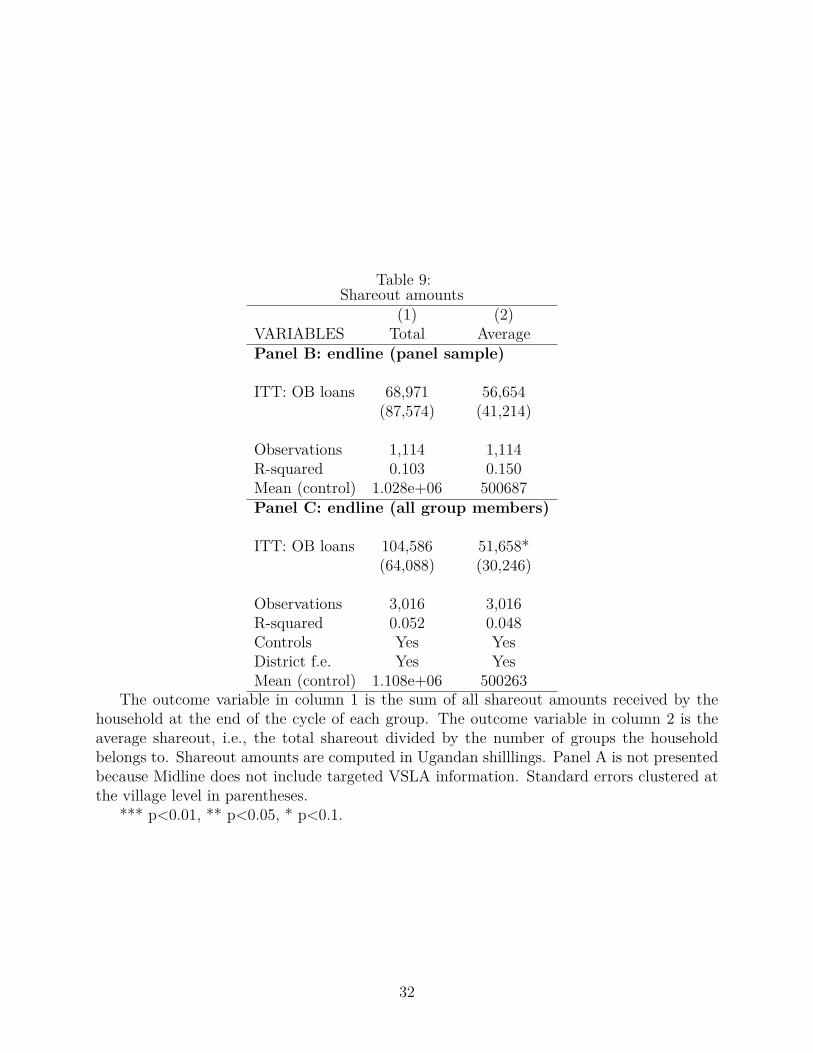
Table 9:Shareout amounts

(1) (2)VARIABLES Total AveragePanel B: endline (panel sample)

ITT: OB loans 68,971 56,654(87,574) (41,214)

Observations 1,114 1,114R-squared 0.103 0.150Mean (control) 1.028e+06 500687Panel C: endline (all group members)

ITT: OB loans 104,586 51,658*(64,088) (30,246)

Observations 3,016 3,016R-squared 0.052 0.048Controls Yes YesDistrict f.e. Yes YesMean (control) 1.108e+06 500263

The outcome variable in column 1 is the sum of all shareout amounts received by thehousehold at the end of the cycle of each group. The outcome variable in column 2 is theaverage shareout, i.e., the total shareout divided by the number of groups the householdbelongs to. Shareout amounts are computed in Ugandan shilllings. Panel A is not presentedbecause Midline does not include targeted VSLA information. Standard errors clustered atthe village level in parentheses.

*** p<0.01, ** p<0.05, * p<0.1.

32

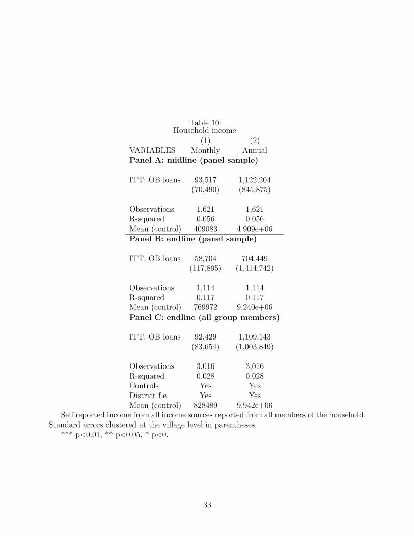
Table 10:Household income

(1) (2)VARIABLES Monthly AnnualPanel A: midline (panel sample)

ITT: OB loans 93,517 1,122,204(70,490) (845,875)

Observations 1,621 1,621R-squared 0.056 0.056Mean (control) 409083 4.909e+06Panel B: endline (panel sample)

ITT: OB loans 58,704 704,449(117,895) (1,414,742)

Observations 1,114 1,114R-squared 0.117 0.117Mean (control) 769972 9.240e+06Panel C: endline (all group members)

ITT: OB loans 92,429 1,109,143(83,654) (1,003,849)

Observations 3,016 3,016R-squared 0.028 0.028Controls Yes YesDistrict f.e. Yes YesMean (control) 828489 9.942e+06

Self reported income from all income sources reported from all members of the household.Standard errors clustered at the village level in parentheses.

*** p<0.01, ** p<0.05, * p<0.

33

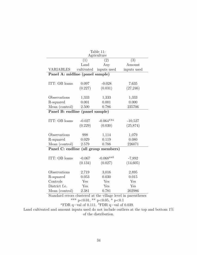
Table 11:Agriculture

(1) (2) (3)Land Any Amount

VARIABLES cultivated inputs used inputs usedPanel A: midline (panel sample)

ITT: OB loans 0.097 -0.028 7,635(0.227) (0.031) (27,246)

Observations 1,333 1,333 1,333R-squared 0.001 0.001 0.000Mean (control) 2.500 0.786 235706Panel B: endline (panel sample)

ITT: OB loans -0.027 -0.064**a -10,527(0.229) (0.030) (25,874)

Observations 998 1,114 1,079R-squared 0.029 0.119 0.080Mean (control) 2.579 0.788 226071Panel C: endline (all group members)

ITT: OB loans -0.067 -0.068**b -7,892(0.134) (0.027) (14,605)

Observations 2,719 3,016 2,895R-squared 0.053 0.030 0.015Controls Yes Yes YesDistrict f.e. Yes Yes YesMean (control) 2.381 0.781 202986Standard errors clustered at the village level in parentheses

*** p<0.01, ** p<0.05, * p<0.1aFDR q−val of 0.111. bFDR q−val of 0.039.

Land cultivated and amount inputs used do not include outliers at the top and bottom 1%of the distribution.

34

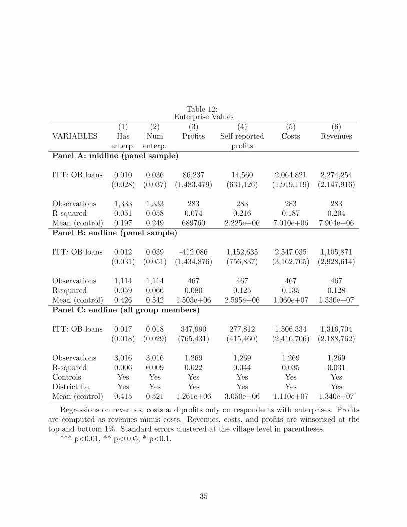
Table 12:Enterprise Values

(1) (2) (3) (4) (5) (6)VARIABLES Has Num Profits Self reported Costs Revenues

enterp. enterp. profitsPanel A: midline (panel sample)

ITT: OB loans 0.010 0.036 86,237 14,560 2,064,821 2,274,254(0.028) (0.037) (1,483,479) (631,126) (1,919,119) (2,147,916)

Observations 1,333 1,333 283 283 283 283R-squared 0.051 0.058 0.074 0.216 0.187 0.204Mean (control) 0.197 0.249 689760 2.225e+06 7.010e+06 7.904e+06Panel B: endline (panel sample)

ITT: OB loans 0.012 0.039 -412,086 1,152,635 2,547,035 1,105,871(0.031) (0.051) (1,434,876) (756,837) (3,162,765) (2,928,614)

Observations 1,114 1,114 467 467 467 467R-squared 0.059 0.066 0.080 0.125 0.135 0.128Mean (control) 0.426 0.542 1.503e+06 2.595e+06 1.060e+07 1.330e+07Panel C: endline (all group members)

ITT: OB loans 0.017 0.018 347,990 277,812 1,506,334 1,316,704(0.018) (0.029) (765,431) (415,460) (2,416,706) (2,188,762)

Observations 3,016 3,016 1,269 1,269 1,269 1,269R-squared 0.006 0.009 0.022 0.044 0.035 0.031Controls Yes Yes Yes Yes Yes YesDistrict f.e. Yes Yes Yes Yes Yes YesMean (control) 0.415 0.521 1.261e+06 3.050e+06 1.110e+07 1.340e+07

Regressions on revenues, costs and profits only on respondents with enterprises. Profitsare computed as revenues minus costs. Revenues, costs, and profits are winsorized at thetop and bottom 1%. Standard errors clustered at the village level in parentheses.

*** p<0.01, ** p<0.05, * p<0.1.

35

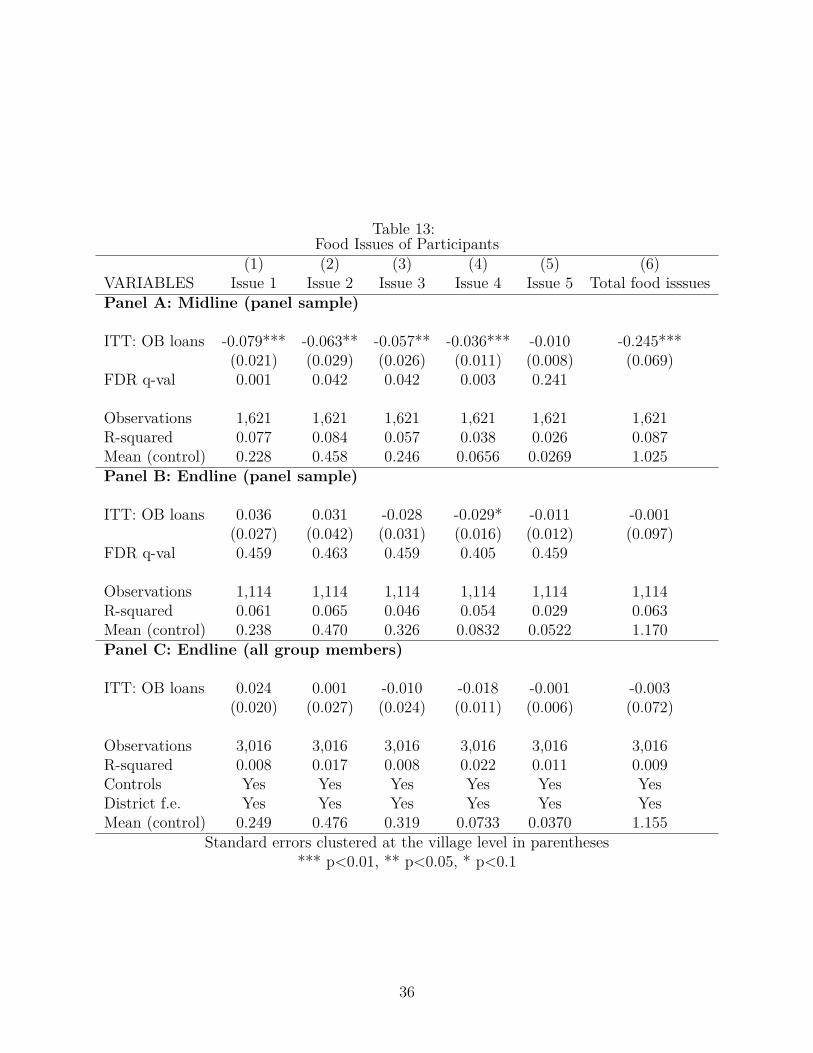
Table 13:Food Issues of Participants

(1) (2) (3) (4) (5) (6)VARIABLES Issue 1 Issue 2 Issue 3 Issue 4 Issue 5 Total food isssuesPanel A: Midline (panel sample)

ITT: OB loans -0.079*** -0.063** -0.057** -0.036*** -0.010 -0.245***(0.021) (0.029) (0.026) (0.011) (0.008) (0.069)

FDR q-val 0.001 0.042 0.042 0.003 0.241

Observations 1,621 1,621 1,621 1,621 1,621 1,621R-squared 0.077 0.084 0.057 0.038 0.026 0.087Mean (control) 0.228 0.458 0.246 0.0656 0.0269 1.025Panel B: Endline (panel sample)

ITT: OB loans 0.036 0.031 -0.028 -0.029* -0.011 -0.001(0.027) (0.042) (0.031) (0.016) (0.012) (0.097)

FDR q-val 0.459 0.463 0.459 0.405 0.459

Observations 1,114 1,114 1,114 1,114 1,114 1,114R-squared 0.061 0.065 0.046 0.054 0.029 0.063Mean (control) 0.238 0.470 0.326 0.0832 0.0522 1.170Panel C: Endline (all group members)

ITT: OB loans 0.024 0.001 -0.010 -0.018 -0.001 -0.003(0.020) (0.027) (0.024) (0.011) (0.006) (0.072)

Observations 3,016 3,016 3,016 3,016 3,016 3,016R-squared 0.008 0.017 0.008 0.022 0.011 0.009Controls Yes Yes Yes Yes Yes YesDistrict f.e. Yes Yes Yes Yes Yes YesMean (control) 0.249 0.476 0.319 0.0733 0.0370 1.155

Standard errors clustered at the village level in parentheses*** p<0.01, ** p<0.05, * p<0.1

36

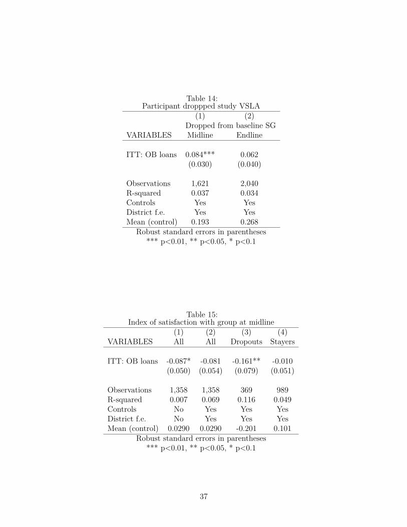
Table 14:Participant droppped study VSLA

(1) (2)Dropped from baseline SG

VARIABLES Midline Endline

ITT: OB loans 0.084*** 0.062(0.030) (0.040)

Observations 1,621 2,040R-squared 0.037 0.034Controls Yes YesDistrict f.e. Yes YesMean (control) 0.193 0.268

Robust standard errors in parentheses*** p<0.01, ** p<0.05, * p<0.1

Table 15:Index of satisfaction with group at midline

(1) (2) (3) (4)VARIABLES All All Dropouts Stayers

ITT: OB loans -0.087* -0.081 -0.161** -0.010(0.050) (0.054) (0.079) (0.051)

Observations 1,358 1,358 369 989R-squared 0.007 0.069 0.116 0.049Controls No Yes Yes YesDistrict f.e. No Yes Yes YesMean (control) 0.0290 0.0290 -0.201 0.101

Robust standard errors in parentheses*** p<0.01, ** p<0.05, * p<0.1

37