Embed Size (px)
Citation preview
Working Paper/Document de travail 2010-24
Banks, Credit Market Frictions, and Business Cycles
by Ali Dib
2
Bank of Canada Working Paper 2010-24
October 2010
Banks, Credit Market Frictions, and Business Cycles
by
Ali Dib
International Economic Analysis Department Bank of Canada
Ottawa, Ontario, Canada K1A 0G9 [email protected]
Bank of Canada working papers are theoretical or empirical works-in-progress on subjects in economics and finance. The views expressed in this paper are those of the author.
No responsibility for them should be attributed to the Bank of Canada.
ISSN 1701-9397 © 2010 Bank of Canada
ii
Acknowledgements
For their comments and discussions, I am grateful to Ron Alquist, Ricardo Caballero, Lawrence Christiano, Carlos de Resende, Brigitte Desroches, Andrea Gerali, Sharon Kozicki, Robert Lafrance, Philipp Maier, Federico Mandelman, Virginia Queijo von Heideken, Julio Rotemberg, Francisco Ruge-Murcia, Eric Santor, Lawrence Schembri, Jack Selody, Moez Souissi, Skander Van den Heuvel, seminar participants at the Bank of Canada, MIT, the IMF, Federal Reserve Bank of Richmond, Federal Reserve Bank of Atlanta, Reserve Bank of Australia, the European Central Bank, Sveriges Riksbank, the Deutsche Bundesbank, Australian National University, University of Ottawa, Dalhousie University, and participants at the BIS/ECB workshop on “Monetary Policy and Financial Stability,” the Bank of Canada/IMF workshop on “Economic Modelling and the Financial Crisis,” the 2009 NBER/Federal Reserve Bank of Philadelphia workshop on “Methods and Applications for the DSGE Models,” the CEA, and the CEF.
iii
Abstract
The author proposes a micro-founded framework that incorporates an active banking sector into a dynamic stochastic general-equilibrium model with a financial accelerator. He evaluates the role of the banking sector in the transmission and propagation of the real effects of aggregate shocks, and assesses the importance of financial shocks in U.S. business cycle fluctuations. The banking sector consists of two types of profit-maximizing banks that offer different banking services and transact in an interbank market. Loans are produced using interbank borrowing and bank capital subject to a regulatory capital requirement. Banks have monopoly power, set nominal deposit and prime lending rates, choose their leverage ratio and their portfolio composition, and can endogenously default on a fraction of their interbank borrowing. Because it is costly to raise capital to satisfy the regulatory capital requirement, the banking sector attenuates the real effects of financial shocks, reduces macroeconomic volatilities, and helps stabilize the economy. The model also includes two unconventional monetary policies (quantitative and qualitative easing) that reduce the negative impacts of financial crises.
JEL classification: E32, E44, G1 Bank classification: Economic models; Business fluctuations and cycles; Credit and credit aggregates; Financial stability
Résumé
L’auteur propose un cadre aux fondements microéconomiques qui intègre un secteur bancaire actif dans un modèle d’équilibre général dynamique et stochastique avec accélérateur financier. Il évalue le rôle du secteur bancaire dans la transmission et la propagation des effets réels des chocs globaux et estime l’importance des chocs financiers dans les fluctuations économiques aux États-Unis. Le secteur bancaire est constitué de deux catégories d’établissements qui offrent des services bancaires différents et réalisent des opérations sur un marché interbancaire en cherchant à maximiser leurs profits. Les prêts sont financés par des emprunts interbancaires et des fonds propres, sous réserve du respect d’exigences réglementaires en matière de fonds propres bancaires. Les banques sont en situation de monopole, fixent les taux nominaux applicables aux dépôts et les taux préférentiels nominaux applicables aux prêts, déterminent elles-mêmes leur ratio de levier et la composition de leur portefeuille et peuvent manquer de façon endogène à leurs obligations à l’égard d’une partie de leurs emprunts interbancaires. Étant donné que la mobilisation de fonds propres pour satisfaire aux exigences réglementaires comporte des coûts, le secteur bancaire atténue les effets réels des chocs financiers, réduit les volatilités macroéconomiques et aide à stabiliser l’économie. Le modèle intègre également deux mesures de politique monétaire non traditionnelles (l’assouplissement quantitatif et l’assouplissement direct du crédit) qui diminuent les effets négatifs des crises financières.
Classification JEL : E32, E44, G1 Classification de la Banque : Modèles économiques; Cycles et fluctuations économiques; Crédit et agrégats du crédit; Stabilité financière
1. Introduction
In light of the recent financial crisis, real-financial linkages have become the focus of attention
of an increasing number of papers that aim to develop dynamic stochastic general-equilibrium
(DSGE) models with financial frictions in both the demand and supply side of credit markets.
Such models provide a better understanding of the role of the banking sector in macroeco-
nomic fluctuations, by incorporating a structural framework to examine banks’ behaviour in
the transmission and propagation of aggregate shocks, and to assess the importance of financial
shocks, originating in the banking sector, as a source of the business cycles. Before the finan-
cial crisis, the banking sector was largely ignored in most DSGE models.1 Moreover, in the
literature, financial frictions are usually modelled only on the demand side of credit markets,
using either the Bernanke, Gertler, and Gilchrist (1999, BGG hereafter) financial accelerator
mechanism or the Iacoviello (2005) framework.2 This demand-side focus was influenced by the
Modigliani–Miller theorem, which states that the capital structure of banks is irrelevant for
their lending decisions.
This paper proposes a micro-founded framework that incorporates an active banking sector,
which includes an interbank market and banks subject to a capital requirement, into a DSGE
model with a financial accelerator a la BGG.3 Unlike previous studies that incorporate bank
capital to solve the moral hazard problem between households and banks, this paper introduces
bank capital to satisfy the capital requirement exogenously imposed by regulators.4 It is a
precondition for banks to operate and provide loans to entrepreneurs. This requirement causes
bank capital to attenuate the real effects of aggregate shocks, rather than act as an amplification
mechanism as in previous studies. For instance, in the event of a positive shock, an increase in
borrowing demand by entrepreneurs forces banks to increase their leverage ratio and/or bank
capital holdings to be able to extend their loan supply. A higher leverage ratio and/or higher1Some recent exceptions are Goodfriend and McCallum (2007); Markovic (2006); and Van den Heuvel (2009).2For example, Carlstrom and Fuerst (1997); Cespedes, Chang, and Velasco (2004); Faia and Monacelli
(2007); Christensen and Dib (2008); De Graeve (2008); Queijo von Heideken (2009). Nevertheless, Christiano,Eichenbaum, and Evans (2005) totally abstract from the financial frictions in their model.
3This framework is fully micro-founded in the sense that all banks maximize profits and take optimal decisionsunder different constraints.
4Examples of these studies are Holmstrom and Tirole (1997); Gertler and Kiyotaki (2010); Goodfriend andMcCallum (2007); Markovic (2006); Zhang (2009); Meh and Moran (2010).
1
bank capital imply higher marginal costs of raising bank capital and, thus, higher marginal
costs of producing loans. Banks transfer these additional costs to entrepreneurs by charging
a higher lending rate. This increases external financing costs and erodes part of the initial
demand from entrepreneurs for loans to finance new investment. Consequently, the increase in
investment and output will be smaller in the presence of the capital requirement.5
This paper is related to the following studies: Goodhart, Sunirand, and Tsomocos (2006);
Curdia and Woodford (2009); de Walque, Pierrard, and Rouabah (2010); Christiano, Motto
and Rostagno (2010); Gerali et al. (2010); Gertler and Karadi (2010); Gertler and Kiyotaki
(2010). Our model is a DSGE model for a closed economy based on BGG. The key innovation
is formally modelling an active banking sector that includes an interbank market and imposes
a regulatory capital requirement. The model incorporates an optimizing banking sector with
two types of monopolistically competitive banks: “savings banks” and “lending banks.” Banks
supply different banking services and transact in the interbank market.6 Savings banks are
financial intermediaries that are net lenders (creditors) in the interbank market, whereas lending
banks are net borrowers (debtors). Banks have monopoly power when setting nominal deposit
and prime lending rates, but subject to quadratic adjustment costs.
Savings banks collect deposits from workers, set nominal deposit rates, and optimally choose
the composition of their portfolio (composed of government bonds and risky interbank lending).
Lending banks borrow from savings banks in the interbank market and raise bank capital (eq-
uity) from households (shareholders) in the financial market to satisfy the capital requirement.
In addition, lending banks optimally choose their leverage ratio; that is, the ratio of loans
to bank capital subject to the maximum leverage ratio imposed by regulators. We assume that
banks that hold capital in excess of the required level receive convex gains.7 This implies that
variations in the banks’ leverage ratio directly affect the marginal cost of raising bank capital.
Therefore, movements in the banks’ leverage ratio may have substantial effects on business
cycle fluctuations, as pointed out by Fostel and Geanakoplos (2008) and Geanakoplos (2009).
Following Goodhart, Sunirand, and Tsomocos (2006), we assume endogenous strategic defaults5Van den Heuvel (2008) studies the welfare cost of bank capital requirement in a DSGE model.6The two different banks are necessary to generate heterogeneity, which in turn leads to an interbank market
where different banks can interact.7The cost of bank capital depends on the bank’s capital position. If banks hold excess bank capital, the
marginal cost of raising equity in the financial market will be lower, since banks are well capitalized.
2
on interbank borrowing. Also, as in Gertler and Kiyotaki (2010), lending banks’ managers can
divert a fraction of bank capital received from shareholders for their own benefit. Nevertheless,
when defaulting on interbank borrowing or diverting a fraction of bank capital, lending banks
must pay convex penalties in the next period. Finally, to introduce unconventional (quanti-
tative and qualitative) monetary policies in the model, we assume that the lending banks can
receive, if needed, injections of money from the central bank and/or swap a fraction of their
loans (risky assets) for government bonds.8
In this framework, variations in a bank’s balance sheet can affect credit supply conditions
and, thus, the real economy through the following channels: (1) variations in the marginal cost
of raising bank capital; (2) the optimal choice of the banks’ leverage ratio subject to the capital
requirement; (3) monopoly power in setting nominal deposit and lending interest rates with
nominal rigidities, implying time-varying interest rate spreads over business cycles;9 (4) the
optimal allocation of the banks’ portfolios between interbank lending (risky assets) and risk-
free asset holdings; and (5) the default risk channels that arise from the endogenous default on
interbank borrowing and diversion of a fraction of bank capital.
The economy is subject to supply and demand shocks, financial shocks (riskiness and the
financial intermediation process), and unconventional monetary policy shocks. The supply
and demand shocks are similar to those commonly used in the literature; however, financial
shocks require some explanation. Riskiness shocks are modelled as shocks to the elasticity of
the risk premium that affect the external finance costs of entrepreneurs. They are meant to
represent shocks to the standard deviation of the entrepreneurial distribution, as in Christiano,
Motto, and Rostagno (2010); shocks to agency costs paid by lending banks to monitor the
entrepreneurs’ output; and/or shocks to the entrepreneurs’ default threshold.10 Shocks to the
financial intermediation process are exogenous events that affect the credit supply of lending
banks. They may represent technological advances or disruptions in the intermediation process,8Quantitative monetary easing, which is associated with newly created money, expands banks’ balance sheets;
qualitative monetary easing (swapping banks’ assets for government bonds) changes only banks’ assets compo-sitions.
9See Curdia and Woodford (2009) for the importance of time-varying spreads on monetary policy.10As shown in BGG, the elasticity of the external finance premium to the entrepreneurs’ leverage ratio depends
on the standard deviation of the entrepreneurial distribution, the agency cost parameter, and entrepreneurs’default threshold.
3
or approximate perceived changes in creditworthiness.11 Finally, unconventional monetary
policy shocks include quantitative and qualitative monetary easing shocks used by the central
banks to provide liquidity to the banking system and to ease financial conditions during times
of financial crises.
The model is calibrated to the U.S. economy and used to evaluate the role of the banking
sector in the transmission and propagation of the real effects of aggregate shocks, to assess
the importance of financial shocks in the U.S. business cycle fluctuations, and to examine the
potential role of unconventional monetary policies in offsetting the negative impacts of financial
crises.
The model is successful in reproducing most of the salient features of the U.S. economy:
key macroeconomic volatilities, autocorrelations, and correlations with output. Importantly,
the impulse responses of key macro variables to different shocks show that, under the capital
requirement, the active banking sector attenuates the real effects of aggregate shocks, particu-
larly financial shocks, and thus helps stabilize the economy. Moreover, the dynamic effects of
financial shocks originating in the banking sector have substantial impacts on the U.S. business
cycles, and could be a substantial source of macroeconomic fluctuations. We also find that bank
leverage is procyclical, indicating that banks are willing to expand more loans during booms
and tend to restrict their supply of credit during recessions.
This paper is organized as follows. In section 2, we describe the model. In section 3, we
discuss the parameter calibration. In section 4, we report and discuss the empirical results.
Section 5 offers some conclusions.
2. The Model
The model has two types of households (workers and bankers) that differ in their degrees of
risk aversion and in the access to financial markets. The banking sector consists of two types
of heterogeneous monopolistically competitive banks. We call them “savings” and “lending”
banks, to indicate that they offer different banking services but interact in an interbank market.
As in BGG, the production sector consists of entrepreneurs, capital producers, and retailers.11Examples of shocks to the financial intermediation process are advances in financial engineering, credit
rationing, and highly sophisticated methods for sharing risk.
4

Finally, there is a central bank and a government.
2.1 Households
2.1.1 Workers
Workers derive utility from total consumption, Cwt , and leisure, 1−Ht, where Ht denotes hours
worked. The workers’ preferences are described by the following expected utility function:
V w0 = E0
∞∑
t=0
βtwu (Cw
t ,Ht) . (1)
The single-period utility is
u(·) =et
1− γw
(Cw
t
(Cwt−1)
ϕ
)1−γw
+η(1−Ht)
1− ς
1−ς
, (2)
where ϕ ∈ (0, 1) is a habit formation parameter, γw is a positive parameter denoting the
workers’ risk aversion, and ς is the inverse of the Frisch wage elasticity of labour supply. The
parameter η measures the weight on leisure in the utility function. et is a preference shock that
is common to workers and bankers, and follows an AR(1) process.
The representative worker enters period t with Dt−1 units of real deposits in savings banks.
Deposits pay the gross nominal interest rate RDt set by savings banks. During period t, workers
supply labour to the entrepreneurs, for which they receive real labour payment WtHt, (Wt is
the economy-wide real wage). Furthermore, they receive dividend payments, ΠRt , from retail
firms, as well as a lump-sum transfer from the monetary authority, Tt, and they pay lump-sum
taxes to the government, Twt . Workers allocate their funds to private consumption and real
deposits, Dt. Their budget constraint in real terms is
Cwt + Dt ≤ WtHt +
RDt−1Dt−1
πt+ ΠR
t + Tt − Twt , (3)
where πt = Pt/Pt−1 is the gross inflation rate. A representative worker chooses Cwt , Ht, and
Dt to maximize the expected lifetime utility, equation (1), subject to the single-period utility
function, equation (2), and the budget constraint, equation (3). The first-order conditions of
this optimization problem are reported in Appendix A.
5
2.1.2 Bankers
Bankers are the owners of the two types of banks, from which they receive profits. They
consume, save in government bonds, and accumulate bank capital supplied to lending banks.
Their preferences depend only on consumption and are given by
V b0 = E0
∞∑
t=0
βtbu
(Cb
t
). (4)
The single-period utility function is
u(·) =et
1− γb
(Cb
t
(Cbt−1)
ϕ
)1−γb
, (5)
where γb is a positive structural parameter denoting bankers’ risk aversion.
Bankers enter period t with (1 − δZt−1)Zt−1 units of the stock of bank capital, whose price
is QZt in period t, where δZ
t−1 is the fraction of bank capital diverted by lending bank managers
in t − 1, and Zt is the volume of bank equity (shares) held by bankers. Bank capital pays a
contingent nominal return rate (dividend), RZt . Bankers also enter period t with Bt−1 units
of government bonds that pay the risk-free nominal interest rate Rt. During period t, bankers
receive profit payments, Πsbt and Πlb
t , from savings and lending banks, and pay lump-sum taxes
to government, T bt . They allocate these funds to consumption, Cb
t , government bonds, Bt, and
bank capital, Zt. We assume that bankers pay costs when adjusting their stock of bank capital
across periods.12 Formally, the adjustment costs are given by
AdjZt =
χZ
2
(Zt
Zt−1− 1
)2
QZt Zt, (6)
where χZ is a positive parameter determining the bank capital adjustment costs. The bankers’
budget constraint, in real terms, is
Cbt + QZ
t Zt + Bt =Rt−1Bt−1
πt+
RZt (1− δZ
t−1)QZt Zt−1
πt−AdjZ
t + Πsbt + Πlb
t − T bt . (7)
12We interpret these adjustment costs as costs paid to brokers, or the costs of collecting information aboutthe banks’ balance sheet.
6
A representative banker chooses Cbt , Bt, and Zt in order to maximize the expected lifetime
utility equation (4), subject to equations (5)–(7). The first-order conditions for this optimiza-
tion problem are:
et
(Cb
t
(Cbt−1)
ϕ
)1−γb
− βbϕEt
et+1
(Cb
t+1
(Cbt )
ϕ
)1−γb = Cb
t λbt ; (8)
λbt
Rt= βbEt
[λb
t+1
πt+1
]; (9)
βbEt
{λw
t+1QZt+1
πt+1
[(1− δZ
t )RZt+1 + χZ
(Zt+1
Zt− 1
)(Zt+1
Zt
)2
πt+1
]}
= λwt QZ
t
[1 + χZ
(Zt
Zt−1− 1
)Zt
Zt−1
]; (10)
where λbt is the Lagrangian multiplier associated with the bankers’ budget constraint.
Equation (8) determines the marginal utility of the bankers’ consumption. Equation (9)
relates the marginal rate of substitution to the real risk-free rate. Finally, equation (10) corre-
sponds to the optimal dynamic evolution of the stock of bank capital. Combining conditions (9)
and (10) yields the following condition relating the expected return on bank capital, EtRZt+1,
to the risk-free rate, Rt, the diversion on bank capital, δZt , and the current costs/future gains
of adjusting the stock of bank capital:
Et
{QZ
t+1
QZt
[(1− δZ
t )RZt+1 + χZ
(Zt+1
Zt− 1
)(Zt+1
Zt
)2
πt+1
]}
= Rt
[1 + χZ
(Zt
Zt−1− 1
)Zt
Zt−1
]. (11)
This condition leads to three channels, through which changes in bank capital affect the
real economy. The first is the price expectation channel, which arises from expectations of
capital gains or losses from holding bank capital shares, due to expected changes in the price
of bank capital Et
[QZ
t+1/QZt
]. The second is the adjustment cost channel, which is a result of
asymmetric information between bankers and banks. The presence of adjustment costs is nec-
essary to reflect asymmetric information, and the adjustment costs are interpreted as costs to
enter into the bank capital market. The third channel is the diversion risk channel that arises
from the existence of the possibility that banks’ managers divert a fraction δZt of bank capital
7
repayment to their own benefits. Therefore, movements in bank capital, caused by macroeco-
nomic fluctuations, have direct impacts on bank capital accumulation and, consequently, on
credit supply conditions.
2.2 Banking sector
The banking sector consists of two types of heterogeneous profit-maximizing banks: savings
and lending banks.
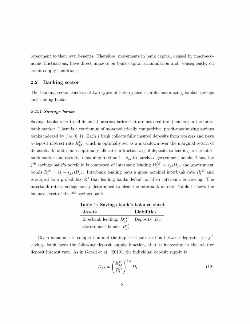
2.2.1 Savings banks
Savings banks refer to all financial intermediaries that are net creditors (lenders) in the inter-
bank market. There is a continuum of monopolistically competitive, profit-maximizing savings
banks indexed by j ∈ (0, 1). Each j bank collects fully insured deposits from workers and pays
a deposit interest rate RDj,t, which is optimally set as a markdown over the marginal return of
its assets. In addition, it optimally allocates a fraction sj,t of deposits to lending in the inter-
bank market and uses the remaining fraction 1− sj,t to purchase government bonds. Thus, the
jth savings bank’s portfolio is composed of interbank lending DIBj,t = sj,tDj,t and government
bonds Bsbt = (1 − sj,t)Dj,t. Interbank lending pays a gross nominal interbank rate RIB
t and
is subject to a probability δDt that lending banks default on their interbank borrowing. The
interbank rate is endogenously determined to clear the interbank market. Table 1 shows the
balance sheet of the jth savings bank.
Table 1: Savings bank’s balance sheet
Assets Liabilities
Interbank lending: DIBj,t Deposits: Dj,t
Government bonds: Bsbj,t
Given monopolistic competition and the imperfect substitution between deposits, the jth
savings bank faces the following deposit supply function, that is increasing in the relative
deposit interest rate. As in Gerali et al. (2010), the individual deposit supply is
Dj,t =
(RD
j,t
RDt
)ϑD
Dt, (12)
8
where Dj,t is deposits supplied to bank j, while Dt denotes total deposits in the economy, and
ϑD > 1 is the elasticity of substitution between different types of deposits.13
Savings banks face quadratic adjustment costs a la Rotemberg (1982) when adjusting the
deposit interest rate:
AdRD
j,t =φRD
2
(RD
j,t
RDj,t−1
− 1
)2
Dt, (13)
where φRD > 0 is an adjustment cost parameter. These adjustment costs imply an interest rate
spread, between deposit and policy rates, that varies over the business cycle. In addition, we
assume that savings banks must pay monitoring costs when lending in the interbank market.
They incur higher monitoring costs if the share sj,t of deposits lent in the interbank market
deviates from a target level s. The individual cost of monitoring interbank lending is
∆sj,t =
χs
2((sj,t − s)Dj,t)
2 , (14)
where χs is a positive parameter determining the steady-state value of the monitoring costs.
Formally, the jth savings bank’s optimization problem is:
max{sj,t,RD
j,t}E0
∞∑
t=0
βtbλ
bt
{[sj,tR
IBt (1− δD
t ) + (1− sj,t)Rt −RDj,t
]Dj,t −AdRD
j,t −∆sj,t
},
subject to equations (12)–(14).14 Since bankers are the owners of banks, the discount factor
is the stochastic process βtbλ
bt , where λb
t denotes the marginal utility of bankers’ consumption.
The term sj,tRIBt (1− δD
t ) + (1− sj,t)Rt is the gross nominal return of savings banks’ assets.
13This supply function is derived from the definition of the aggregate supply of deposits, Dt, and the corre-sponding deposit interest rate, RD
t , in the monopolistic competition framework, as follows:
Dt =
(∫ 1
0D
1+ϑDϑD
j,t dj
) ϑDϑD+1
and RDt =
(∫ 1
0RD
j,t1+ϑD dj
) 11+ϑD , where Dj,t and RD
j,t are, respectively, the supply
and deposit interest rates faced by each savings bank j ∈ (0, 1).14Savings banks take RIB
t , Rt, and δDt as given when maximizing their profits.
9
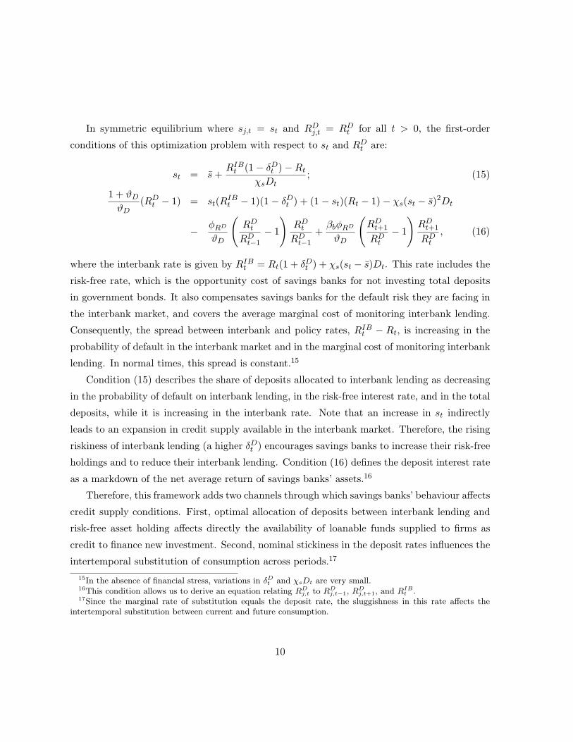
In symmetric equilibrium where sj,t = st and RDj,t = RD
t for all t > 0, the first-order
conditions of this optimization problem with respect to st and RDt are:
st = s +RIB
t (1− δDt )−Rt
χsDt; (15)
1 + ϑD
ϑD(RD
t − 1) = st(RIBt − 1)(1− δD
t ) + (1− st)(Rt − 1)− χs(st − s)2Dt
− φRD
ϑD
(RD
t
RDt−1
− 1
)RD
t
RDt−1
+βbφRD
ϑD
(RD
t+1
RDt
− 1
)RD
t+1
RDt
, (16)
where the interbank rate is given by RIBt = Rt(1 + δD
t ) + χs(st − s)Dt. This rate includes the
risk-free rate, which is the opportunity cost of savings banks for not investing total deposits
in government bonds. It also compensates savings banks for the default risk they are facing in
the interbank market, and covers the average marginal cost of monitoring interbank lending.
Consequently, the spread between interbank and policy rates, RIBt − Rt, is increasing in the
probability of default in the interbank market and in the marginal cost of monitoring interbank
lending. In normal times, this spread is constant.15
Condition (15) describes the share of deposits allocated to interbank lending as decreasing
in the probability of default on interbank lending, in the risk-free interest rate, and in the total
deposits, while it is increasing in the interbank rate. Note that an increase in st indirectly
leads to an expansion in credit supply available in the interbank market. Therefore, the rising
riskiness of interbank lending (a higher δDt ) encourages savings banks to increase their risk-free
holdings and to reduce their interbank lending. Condition (16) defines the deposit interest rate
as a markdown of the net average return of savings banks’ assets.16
Therefore, this framework adds two channels through which savings banks’ behaviour affects
credit supply conditions. First, optimal allocation of deposits between interbank lending and
risk-free asset holding affects directly the availability of loanable funds supplied to firms as
credit to finance new investment. Second, nominal stickiness in the deposit rates influences the
intertemporal substitution of consumption across periods.17
15In the absence of financial stress, variations in δDt and χsDt are very small.
16This condition allows us to derive an equation relating RDj,t to RD
j,t−1, RDj,t+1, and RIB
t .17Since the marginal rate of substitution equals the deposit rate, the sluggishness in this rate affects the
intertemporal substitution between current and future consumption.
10
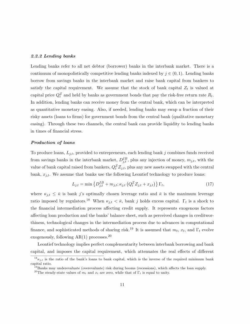
2.2.2 Lending banks
Lending banks refer to all net debtor (borrower) banks in the interbank market. There is a
continuum of monopolistically competitive lending banks indexed by j ∈ (0, 1). Lending banks
borrow from savings banks in the interbank market and raise bank capital from bankers to
satisfy the capital requirement. We assume that the stock of bank capital Zt is valued at
capital price QZt and held by banks as government bonds that pay the risk-free return rate Rt.
In addition, lending banks can receive money from the central bank, which can be interpreted
as quantitative monetary easing. Also, if needed, lending banks may swap a fraction of their
risky assets (loans to firms) for government bonds from the central bank (qualitative monetary
easing). Through these two channels, the central bank can provide liquidity to lending banks
in times of financial stress.
Production of loans
To produce loans, Lj,t, provided to entrepreneurs, each lending bank j combines funds received
from savings banks in the interbank market, DIBj,t , plus any injection of money, mj,t, with the
value of bank capital raised from bankers, QZt Zj,t, plus any new assets swapped with the central
bank, xj,t. We assume that banks use the following Leontief technology to produce loans:
Lj,t = min{DIB
j,t + mj,t;κj,t
(QZ
t Zj,t + xj,t
)}Γt, (17)
where κj,t ≤ κ is bank j’s optimally chosen leverage ratio and κ is the maximum leverage
ratio imposed by regulators.18 When κj,t < κ, bank j holds excess capital. Γt is a shock to
the financial intermediation process affecting credit supply. It represents exogenous factors
affecting loan production and the banks’ balance sheet, such as perceived changes in creditwor-
thiness, technological changes in the intermediation process due to advances in computational
finance, and sophisticated methods of sharing risk.19 It is assumed that mt, xt, and Γt evolve
exogenously, following AR(1) processes.20
Leontief technology implies perfect complementarity between interbank borrowing and bank
capital, and imposes the capital requirement, which attenuates the real effects of different18κj,t is the ratio of the bank’s loans to bank capital, which is the inverse of the required minimum bank
capital ratio.19Banks may underevaluate (overevaluate) risk during booms (recessions), which affects the loan supply.20The steady-state values of mt and xt are zero, while that of Γt is equal to unity.
11
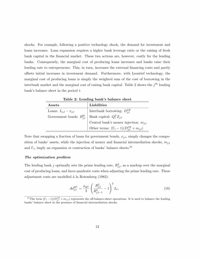
shocks. For example, following a positive technology shock, the demand for investment and
loans increases. Loan expansion requires a higher bank leverage ratio or the raising of fresh
bank capital in the financial market. These two actions are, however, costly for the lending
banks. Consequently, the marginal cost of producing loans increases and banks raise their
lending rate to entrepreneurs. This, in turn, increases the external financing costs and partly
offsets initial increases in investment demand. Furthermore, with Leontief technology, the
marginal cost of producing loans is simply the weighted sum of the cost of borrowing in the
interbank market and the marginal cost of raising bank capital. Table 2 shows the jth lending
bank’s balance sheet in the period t.
Table 2: Lending bank’s balance sheet
Assets Liabilities
Loans: Lj,t − xj,t Interbank borrowing: DIBj,t
Government bonds: Blbj,t Bank capital: QZ
t Zj,t
Central bank’s money injection: mj,t
Other terms: (Γt − 1)(DIBj,t + mj,t)
Note that swapping a fraction of loans for government bonds, xj,t, simply changes the compo-
sition of banks’ assets, while the injection of money and financial intermediation shocks, mj,t
and Γt, imply an expansion or contraction of banks’ balance sheets.21
The optimization problem
The lending bank j optimally sets the prime lending rate, RLj,t, as a markup over the marginal
cost of producing loans, and faces quadratic costs when adjusting the prime lending rate. These
adjustment costs are modelled a la Rotemberg (1982):
AdRL
j,t =φRL
2
(RL
j,t
RLj,t−1
− 1
)2
Lt, (18)
21The term (Γt− 1)(DIBj,t +mj,t) represents the off-balance-sheet operations. It is used to balance the lending
banks’ balance sheet in the presence of financial intermediation shocks.
12
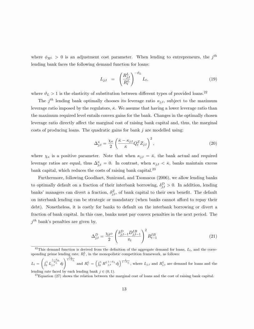
where φRL > 0 is an adjustment cost parameter. When lending to entrepreneurs, the jth
lending bank faces the following demand function for loans:
Lj,t =
(RL
j,t
RLt
)−ϑL
Lt, (19)
where ϑL > 1 is the elasticity of substitution between different types of provided loans.22
The jth lending bank optimally chooses its leverage ratio κj,t, subject to the maximum
leverage ratio imposed by the regulators, κ. We assume that having a lower leverage ratio than
the maximum required level entails convex gains for the bank. Changes in the optimally chosen
leverage ratio directly affect the marginal cost of raising bank capital and, thus, the marginal
costs of producing loans. The quadratic gains for bank j are modelled using:
∆κj,t =
χκ
2
(κ− κj,t
κQZ
t Zj,t
)2
, (20)
where χκ is a positive parameter. Note that when κj,t = κ, the bank actual and required
leverage ratios are equal, thus ∆κj,t = 0. In contrast, when κj,t < κ, banks maintain excess
bank capital, which reduces the costs of raising bank capital.23
Furthermore, following Goodhart, Sunirand, and Tsomacos (2006), we allow lending banks
to optimally default on a fraction of their interbank borrowing, δDj,t > 0. In addition, lending
banks’ managers can divert a fraction, δZj,t, of bank capital to their own benefit. The default
on interbank lending can be strategic or mandatary (when banks cannot afford to repay their
debt). Nonetheless, it is costly for banks to default on the interbank borrowing or divert a
fraction of bank capital. In this case, banks must pay convex penalties in the next period. The
jth bank’s penalties are given by,
∆Dj,t =
χδD
2
(δDj,t−1D
IBj,t−1
πt
)2
RIBt−1 (21)
22This demand function is derived from the definition of the aggregate demand for loans, Lt, and the corre-sponding prime lending rate, RL
t , in the monopolistic competition framework, as follows:
Lt =
(∫ 1
0L
1−ϑLϑL
j,t dj
) ϑL1−ϑL
and RLt =
(∫ 1
0RL1−ϑL
j,t dj) 1
1−ϑL , where Lj,t and RLj,t are demand for loans and the
lending rate faced by each lending bank j ∈ (0, 1).23Equation (27) shows the relation between the marginal cost of loans and the cost of raising bank capital.
13
and
∆Zj,t =
χδZ
2
(δZj,t−1Q
Zt−1Zj,t−1
πt
)2
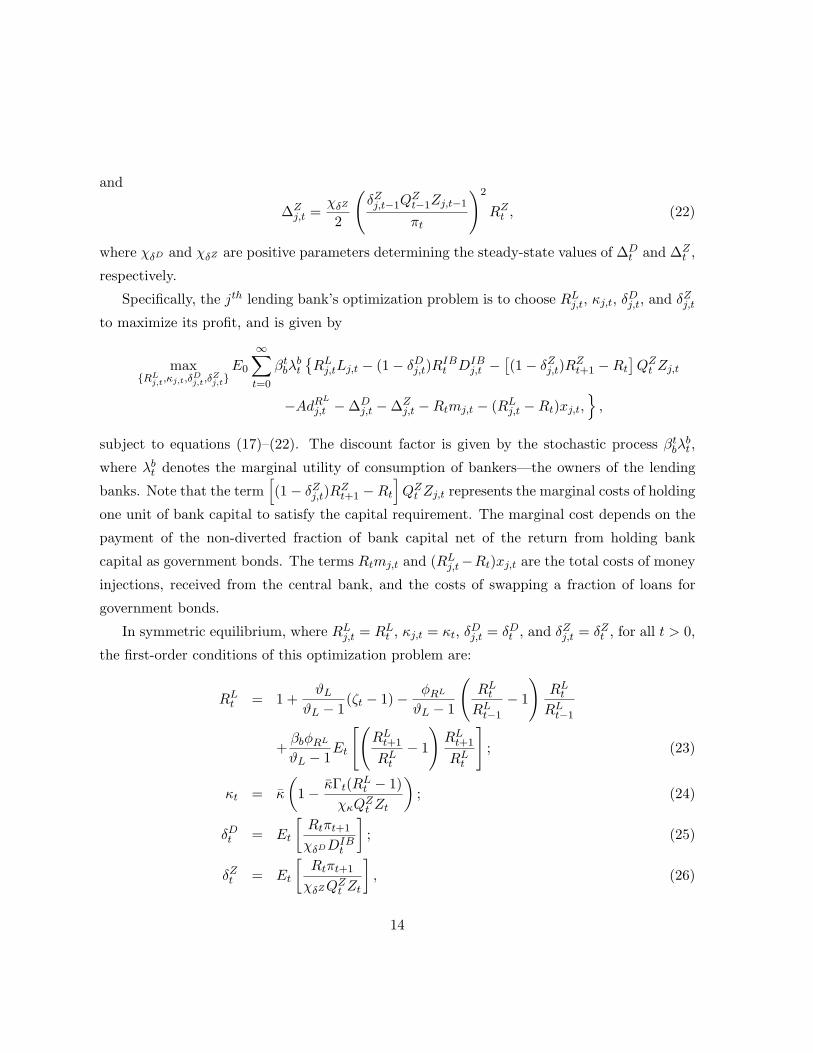
RZt , (22)
where χδD and χδZ are positive parameters determining the steady-state values of ∆Dt and ∆Z
t ,
respectively.
Specifically, the jth lending bank’s optimization problem is to choose RLj,t, κj,t, δD
j,t, and δZj,t
to maximize its profit, and is given by
max{RL
j,t,κj,t,δDj,t,δ
Zj,t}
E0
∞∑
t=0
βtbλ
bt
{RL
j,tLj,t − (1− δDj,t)R
IBt DIB
j,t −[(1− δZ
j,t)RZt+1 −Rt
]QZ
t Zj,t
−AdRL
j,t −∆Dj,t −∆Z
j,t −Rtmj,t − (RLj,t −Rt)xj,t,
},
subject to equations (17)–(22). The discount factor is given by the stochastic process βtbλ
bt ,
where λbt denotes the marginal utility of consumption of bankers—the owners of the lending
banks. Note that the term[(1− δZ
j,t)RZt+1 −Rt
]QZ
t Zj,t represents the marginal costs of holding
one unit of bank capital to satisfy the capital requirement. The marginal cost depends on the
payment of the non-diverted fraction of bank capital net of the return from holding bank
capital as government bonds. The terms Rtmj,t and (RLj,t−Rt)xj,t are the total costs of money
injections, received from the central bank, and the costs of swapping a fraction of loans for
government bonds.
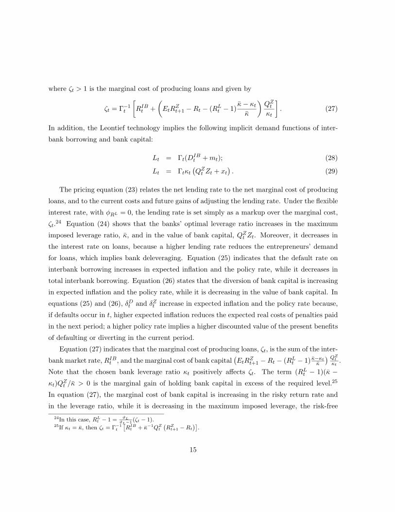
In symmetric equilibrium, where RLj,t = RL
t , κj,t = κt, δDj,t = δD
t , and δZj,t = δZ
t , for all t > 0,
the first-order conditions of this optimization problem are:
RLt = 1 +
ϑL
ϑL − 1(ζt − 1)− φRL
ϑL − 1
(RL
t
RLt−1
− 1
)RL
t
RLt−1
+βbφRL
ϑL − 1Et
[(RL
t+1
RLt
− 1
)RL
t+1
RLt
]; (23)
κt = κ
(1− κΓt(RL
t − 1)χκQZ
t Zt
); (24)
δDt = Et
[Rtπt+1
χδDDIBt
]; (25)
δZt = Et
[Rtπt+1
χδZQZt Zt
], (26)
14
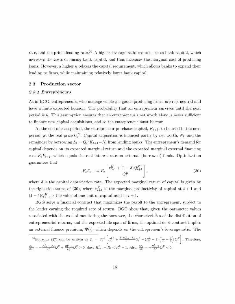
where ζt > 1 is the marginal cost of producing loans and given by
ζt = Γ−1t
[RIB
t +(
EtRZt+1 −Rt − (RL
t − 1)κ− κt
κ
)QZ
t
κt
]. (27)
In addition, the Leontief technology implies the following implicit demand functions of inter-
bank borrowing and bank capital:
Lt = Γt(DIBt + mt); (28)
Lt = Γtκt
(QZ
t Zt + xt
). (29)
The pricing equation (23) relates the net lending rate to the net marginal cost of producing
loans, and to the current costs and future gains of adjusting the lending rate. Under the flexible
interest rate, with φRL = 0, the lending rate is set simply as a markup over the marginal cost,
ζt.24 Equation (24) shows that the banks’ optimal leverage ratio increases in the maximum
imposed leverage ratio, κ, and in the value of bank capital, QZt Zt. Moreover, it decreases in
the interest rate on loans, because a higher lending rate reduces the entrepreneurs’ demand
for loans, which implies bank deleveraging. Equation (25) indicates that the default rate on
interbank borrowing increases in expected inflation and the policy rate, while it decreases in
total interbank borrowing. Equation (26) states that the diversion of bank capital is increasing
in expected inflation and the policy rate, while it is decreasing in the value of bank capital. In
equations (25) and (26), δDt and δZ
t increase in expected inflation and the policy rate because,
if defaults occur in t, higher expected inflation reduces the expected real costs of penalties paid
in the next period; a higher policy rate implies a higher discounted value of the present benefits
of defaulting or diverting in the current period.
Equation (27) indicates that the marginal cost of producing loans, ζt, is the sum of the inter-
bank market rate, RIBt , and the marginal cost of bank capital
(EtR
Zt+1 −Rt − (RL
t − 1) κ−κtκ
) QZt
κt.
Note that the chosen bank leverage ratio κt positively affects ζt. The term (RLt − 1)(κ −
κt)QZt /κ > 0 is the marginal gain of holding bank capital in excess of the required level.25
In equation (27), the marginal cost of bank capital is increasing in the risky return rate and
in the leverage ratio, while it is decreasing in the maximum imposed leverage, the risk-free24In this case, RL
t − 1 = ϑLϑL−1
(ζt − 1).25If κt = κ, then ζt = Γ−1
t
[RIB
t + κ−1QZt
(RZ
t+1 −Rt
)].
15
rate, and the prime lending rate.26 A higher leverage ratio reduces excess bank capital, which
increases the costs of raising bank capital, and thus increases the marginal cost of producing
loans. However, a higher κ relaxes the capital requirement, which allows banks to expand their
lending to firms, while maintaining relatively lower bank capital.
2.3 Production sector
2.3.1 Entrepreneurs
As in BGG, entrepreneurs, who manage wholesale-goods-producing firms, are risk neutral and
have a finite expected horizon. The probability that an entrepreneur survives until the next
period is ν. This assumption ensures that an entrepreneur’s net worth alone is never sufficient
to finance new capital acquisitions, and so the entrepreneur must borrow.
At the end of each period, the entrepreneur purchases capital, Kt+1, to be used in the next
period, at the real price QKt . Capital acquisition is financed partly by net worth, Nt, and the
remainder by borrowing Lt = QKt Kt+1−Nt from lending banks. The entrepreneur’s demand for
capital depends on its expected marginal return and the expected marginal external financing
cost EtFt+1, which equals the real interest rate on external (borrowed) funds. Optimization
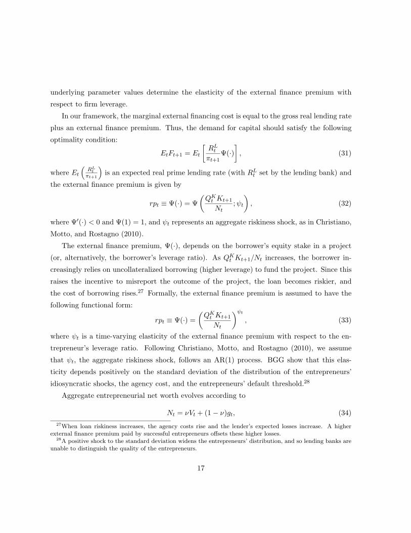
guarantees that
EtFt+1 = Et
[rKt+1 + (1− δ)QK
t+1
QKt
], (30)
where δ is the capital depreciation rate. The expected marginal return of capital is given by
the right-side terms of (30), where rKt+1 is the marginal productivity of capital at t + 1 and
(1− δ)QKt+1 is the value of one unit of capital used in t + 1.
BGG solve a financial contract that maximizes the payoff to the entrepreneur, subject to
the lender earning the required rate of return. BGG show that, given the parameter values
associated with the cost of monitoring the borrower, the characteristics of the distribution of
entrepreneurial returns, and the expected life span of firms, the optimal debt contract implies
an external finance premium, Ψ(·), which depends on the entrepreneur’s leverage ratio. The
26Equation (27) can be written as ζt = Γ−1t
[RIB
t +EtRZ
t+1−Rt
κtQZ
t − (RLt − 1)
(1κt− 1
κ
)QZ
t
]. Therefore,
∂ζt∂κt
= −RZt+1−Rt
κ2t
QZt +
RLt −1
κ2t
QZt > 0, since RZ
t+1 −Rt < RLt − 1. Also, ∂ζt
∂κ= −RL
t −1
κ2 QZt < 0.
16
underlying parameter values determine the elasticity of the external finance premium with
respect to firm leverage.
In our framework, the marginal external financing cost is equal to the gross real lending rate
plus an external finance premium. Thus, the demand for capital should satisfy the following
optimality condition:
EtFt+1 = Et
[RL
t
πt+1Ψ(·)
], (31)
where Et
(RL
tπt+1
)is an expected real prime lending rate (with RL
t set by the lending bank) and
the external finance premium is given by
rpt ≡ Ψ(·) = Ψ(
QKt Kt+1
Nt;ψt
), (32)
where Ψ′(·) < 0 and Ψ(1) = 1, and ψt represents an aggregate riskiness shock, as in Christiano,
Motto, and Rostagno (2010).
The external finance premium, Ψ(·), depends on the borrower’s equity stake in a project
(or, alternatively, the borrower’s leverage ratio). As QKt Kt+1/Nt increases, the borrower in-
creasingly relies on uncollateralized borrowing (higher leverage) to fund the project. Since this
raises the incentive to misreport the outcome of the project, the loan becomes riskier, and
the cost of borrowing rises.27 Formally, the external finance premium is assumed to have the
following functional form:
rpt ≡ Ψ(·) =(
QKt Kt+1
Nt
)ψt
, (33)
where ψt is a time-varying elasticity of the external finance premium with respect to the en-
trepreneur’s leverage ratio. Following Christiano, Motto, and Rostagno (2010), we assume
that ψt, the aggregate riskiness shock, follows an AR(1) process. BGG show that this elas-
ticity depends positively on the standard deviation of the distribution of the entrepreneurs’
idiosyncratic shocks, the agency cost, and the entrepreneurs’ default threshold.28
Aggregate entrepreneurial net worth evolves according to
Nt = νVt + (1− ν)gt, (34)27When loan riskiness increases, the agency costs rise and the lender’s expected losses increase. A higher
external finance premium paid by successful entrepreneurs offsets these higher losses.28A positive shock to the standard deviation widens the entrepreneurs’ distribution, and so lending banks are
unable to distinguish the quality of the entrepreneurs.
17
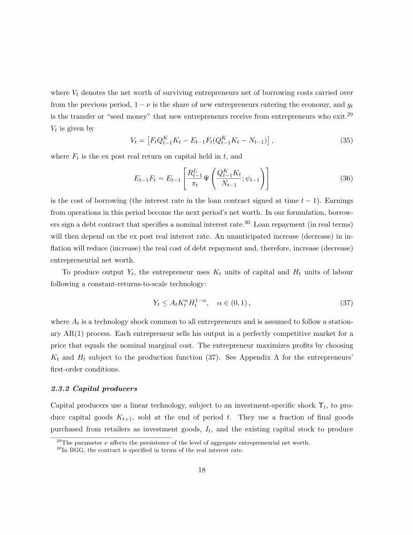
where Vt denotes the net worth of surviving entrepreneurs net of borrowing costs carried over
from the previous period, 1− ν is the share of new entrepreneurs entering the economy, and gt
is the transfer or “seed money” that new entrepreneurs receive from entrepreneurs who exit.29
Vt is given by
Vt =[FtQ
Kt−1Kt −Et−1Ft(QK
t−1Kt −Nt−1)], (35)
where Ft is the ex post real return on capital held in t, and
Et−1Ft = Et−1
[RL
t−1
πtΨ
(QK
t−1Kt
Nt−1;ψt−1
)](36)
is the cost of borrowing (the interest rate in the loan contract signed at time t− 1). Earnings
from operations in this period become the next period’s net worth. In our formulation, borrow-
ers sign a debt contract that specifies a nominal interest rate.30 Loan repayment (in real terms)
will then depend on the ex post real interest rate. An unanticipated increase (decrease) in in-
flation will reduce (increase) the real cost of debt repayment and, therefore, increase (decrease)
entrepreneurial net worth.
To produce output Yt, the entrepreneur uses Kt units of capital and Ht units of labour
following a constant-returns-to-scale technology:
Yt ≤ AtKαt H1−α
t , α ∈ (0, 1) , (37)
where At is a technology shock common to all entrepreneurs and is assumed to follow a station-
ary AR(1) process. Each entrepreneur sells his output in a perfectly competitive market for a
price that equals the nominal marginal cost. The entrepreneur maximizes profits by choosing
Kt and Ht subject to the production function (37). See Appendix A for the entrepreneurs’
first-order conditions.
2.3.2 Capital producers
Capital producers use a linear technology, subject to an investment-specific shock Υt, to pro-
duce capital goods Kt+1, sold at the end of period t. They use a fraction of final goods
purchased from retailers as investment goods, It, and the existing capital stock to produce29The parameter ν affects the persistence of the level of aggregate entrepreneurial net worth.30In BGG, the contract is specified in terms of the real interest rate.
18
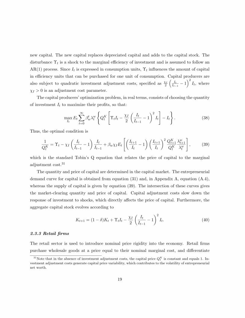
new capital. The new capital replaces depreciated capital and adds to the capital stock. The
disturbance Υt is a shock to the marginal efficiency of investment and is assumed to follow an
AR(1) process. Since It is expressed in consumption units, Υt influences the amount of capital
in efficiency units that can be purchased for one unit of consumption. Capital producers are
also subject to quadratic investment adjustment costs, specified as χI2
(It
It−1− 1
)2It, where
χI > 0 is an adjustment cost parameter.
The capital producers’ optimization problem, in real terms, consists of choosing the quantity
of investment It to maximize their profits, so that:
maxIt
Et
∞∑
t=0
βtwλw
t
{QK
t
[ΥtIt − χI
2
(It
It−1− 1
)2
It
]− It
}. (38)
Thus, the optimal condition is
1QK
t
= Υt − χI
(It
It−1− 1
)It
It−1+ βwχIEt
[(It+1
It− 1
)(It+1
It
)2 QKt+1
QKt
λwt+1
λwt
], (39)
which is the standard Tobin’s Q equation that relates the price of capital to the marginal
adjustment cost.31
The quantity and price of capital are determined in the capital market. The entrepreneurial
demand curve for capital is obtained from equation (31) and, in Appendix A, equation (A.4),
whereas the supply of capital is given by equation (39). The intersection of these curves gives
the market-clearing quantity and price of capital. Capital adjustment costs slow down the
response of investment to shocks, which directly affects the price of capital. Furthermore, the
aggregate capital stock evolves according to
Kt+1 = (1− δ)Kt + ΥtIt − χI
2
(It
It−1− 1
)2
It. (40)
2.3.3 Retail firms
The retail sector is used to introduce nominal price rigidity into the economy. Retail firms
purchase wholesale goods at a price equal to their nominal marginal cost, and differentiate31Note that in the absence of investment adjustment costs, the capital price QK
t is constant and equals 1. In-vestment adjustment costs generate capital price variability, which contributes to the volatility of entrepreneurialnet worth.
19
them at no cost. They then sell these differentiated retail goods in a monopolistically com-
petitive market. Following Calvo (1983) and Yun (1996), we assume that each retailer does
not reoptimize its selling price unless it receives a random signal. The constant probability of
receiving such a signal is (1−φp); and, with probability φp, the retailer j must charge the same
price as in the preceding period, indexed to the steady-state gross rate of inflation, π. At time
t, if the retailer j receives the signal to reoptimize, it chooses a price Pt(j) that maximizes the
discounted, expected real total profits for l periods.
2.4 Central bank and government
2.4.1 Central bank
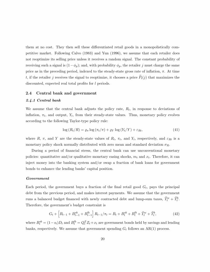
We assume that the central bank adjusts the policy rate, Rt, in response to deviations of
inflation, πt, and output, Yt, from their steady-state values. Thus, monetary policy evolves
according to the following Taylor-type policy rule:
log (Rt/R) = %π log (πt/π) + %Y log (Yt/Y ) + εRt, (41)
where R, π, and Y are the steady-state values of Rt, πt, and Yt, respectively, and εRt is a
monetary policy shock normally distributed with zero mean and standard deviation σR.
During a period of financial stress, the central bank can use unconventional monetary
policies: quantitative and/or qualitative monetary easing shocks, mt and xt. Therefore, it can
inject money into the banking system and/or swap a fraction of bank loans for government
bonds to enhance the lending banks’ capital position.
Government
Each period, the government buys a fraction of the final retail good Gt, pays the principal
debt from the previous period, and makes interest payments. We assume that the government
runs a balanced budget financed with newly contracted debt and lump-sum taxes, Twt + T b
t .
Therefore, the government’s budget constraint is
Gt +[Bt−1 + Bsb
t−1 + Blbt−1
]Rt−1/πt = Bt + Bsb
t + Blbt + Tw
t + T bt , (42)
where Bsbt = (1−st)Dt and Blb
t = QZt Zt+xt are government bonds held by savings and lending
banks, respectively. We assume that government spending Gt follows an AR(1) process.
20
2.5 Markets clearing
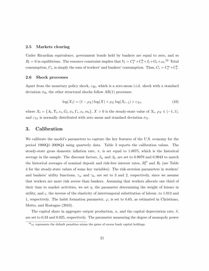
Under Ricardian equivalence, government bonds held by bankers are equal to zero, and so
Bt = 0 in equilibrium. The resource constraint implies that Yt = Cwt +Cb
t +It+Gt+ωt.32 Total
consumption, Ct, is simply the sum of workers’ and bankers’ consumption. Thus, Ct = Cwt +Cb
t .
2.6 Shock processes
Apart from the monetary policy shock, εRt, which is a zero-mean i.i.d. shock with a standard
deviation σR, the other structural shocks follow AR(1) processes:
log(Xt) = (1− ρX) log(X) + ρX log(Xt−1) + εXt, (43)
where Xt = {At, Υt, et, Gt, ψt, Γt, xt, mt}, X > 0 is the steady-state value of Xt, ρX ∈ (−1, 1),
and εXt is normally distributed with zero mean and standard deviation σX .
3. Calibration
We calibrate the model’s parameters to capture the key features of the U.S. economy for the
period 1980Q1–2008Q4 using quarterly data. Table 3 reports the calibration values. The
steady-state gross domestic inflation rate, π, is set equal to 1.0075, which is the historical
average in the sample. The discount factors, βw and βb, are set to 0.9979 and 0.9943 to match
the historical averages of nominal deposit and risk-free interest rates, RDt and Rt (see Table
4 for the steady-state values of some key variables). The risk-aversion parameters in workers’
and bankers’ utility functions, γw and γb, are set to 3 and 2, respectively, since we assume
that workers are more risk averse than bankers. Assuming that workers allocate one third of
their time to market activities, we set η, the parameter determining the weight of leisure in
utility, and ς, the inverse of the elasticity of intertemporal substitution of labour, to 1.013 and
1, respectively. The habit formation parameter, ϕ, is set to 0.65, as estimated in Christiano,
Motto, and Rostagno (2010).
The capital share in aggregate output production, α, and the capital depreciation rate, δ,
are set to 0.33 and 0.025, respectively. The parameter measuring the degree of monopoly power32ωt represents the default penalties minus the gains of excess bank capital holdings.
21
in the retail-goods market θ is set to 6, which implies a 20 per cent markup in the steady-state
equilibrium. The parameters ϑD and ϑL, which measure the degrees of monopoly power of
savings and lending banks, are set equal to 1.53 and 4.21, respectively. These values are set to
match the historical averages of deposit and prime lending rates, RD and RL (see Table 4).
The nominal price rigidity parameter, φp, in the Calvo-Yun price contract is set to 0.75,
implying that the average price remains unchanged for four quarters. This value is estimated
by Christensen and Dib (2008) for the U.S. economy and commonly used in the literature. The
parameters of the adjustment costs of deposit and prime lending interest rates, φRD and φRL ,
are, respectively, set to 40 and 55, to match the standard deviations (volatilities) of the deposit
and prime lending rates to those observed in the data.
Monetary policy parameters %π and %Y are set to values of 1.2 and 0.05, respectively, and
these values satisfy the Taylor principle (see Taylor 1993). The standard deviation of the
monetary policy shock, σR, is the usually estimated value of 0.006.
The investment and bank capital adjustment cost parameters, χI and χZ , are set to 8 and
70, respectively. This is to match the relative volatilities of investment and loans (with respect
to output) to those observed in the data. Similarly, the parameter χs, which determines the
ratio of bank lending to total assets held by the savings banks st, is set to 0.001, so that the
steady-state value of st is equal to 0.82, which corresponds to the historical ratio observed in
the data.33 The parameter χκ is set to 14.45, so that the steady-state value of the bank’s
leverage ratio, κ, is equal to 11.5, which matches the historical average observed in the U.S.
data.
Based on the Basel II minimum required bank capital ratio of 8 per cent, we assume that
the maximum imposed bank leverage, κ, is 12.5.34 Similarly, we calibrate χδD and χδZ , the
parameters determining the total costs of banks’ defaults on interbank borrowing and bank
capital, at 163.1 and 1078, so that the probability of default in the interbank market and the
bank capital diversion are equal to 1 per cent and 1.6 per cent in annual terms (see Table 3).
Following BGG, the steady-state leverage ratio of entrepreneurs, 1 − N/K, is set to 0.5,
matching the historical average. The probability of entrepreneurial survival to the next period,33In the data, the ratio of total government securities held by banks to their assets, 1 − s, is 0.18.34This is because the maximum bank leverage ratio is simply the inverse of the minimum required bank capital
ratio, which is 8 per cent in the Basel II Accord.
22
ν, is set at 0.9833, while ψ, the steady-state elasticity of the external finance premium, is set
at 0.05, the value used by BGG and close to that estimated by Christensen and Dib (2008).35
We calibrate the shocks’ process parameters using either values in previous studies or es-
timated values. The parameters of technology, preference, and investment-specific shocks are
calibrated using the estimated values in Christensen and Dib (2008). To calibrate the param-
eters of the government spending process, we use an OLS estimation of government spending
in real per capita terms (see Appendix B). The estimated value of ρG, the autocorrelation
coefficients, is 0.81, while the estimated standard error, σG, is 0.0166.
To calibrate the parameters of the riskiness shock process ψt, we set the autocorrelation
coefficient ρψ to 0.83, the estimated value in Christiano, Motto, and Rostagno (2010), while
the standard error σψ is set to 0.05 to match the volatility of the external risk premium to that
observed in the data, measured as the difference between Moody’s BAA yield corporate bond
yields and the 3-month T-bill rate. We set the autocorrelation coefficient and the standard
error of financial intermediation process ρΓ and σΓ to 0.8 and 0.003, respectively. These values
are motivated by the potential persistence and low volatility of this financial shock.36 Finally,
we set the autocorrelation coefficients of quantitative and qualitative monetary easing shocks,
ρm and ρx, equal to 0.5, and their standard deviations, σm and σx, to 0.
4. Empirical Results
To assess the role and the importance of banking sector frictions in U.S. business cycle fluctua-
tions, we simulate two alternative models: (1) the above-described model (the baseline model,
hereafter) that incorporates both financial frictions in the banking sector and the financial
accelerator mechanism, and (2) a model that includes only the financial accelerator mechanism
a la BGG (the FA model).37 In addition, as a sensitive analysis exercise, we report the impulse
responses of a constrainted version of the baseline model without the interest rate rigidity (the35Christensen and Dib (2008) estimate ψ at 0.046 for the U.S. economy.36Future work consists of estimating the model’s structural parameters using either a maximum-likelihood
procedure, as used in Christensen and Dib (2008), Ireland (2003), and Dib (2003), or a Bayesien approach, asused in Christiano, Motto, and Rostagno (2010), Dib, Mendicino, and Zhang (2008), Elekdag, Justiniano, andTchakarov (2006), Queijo von Heideken (2009), and others.
37Note that, besides the external risk premium, the external financing cost depends on the prime lending ratein the baseline model, while it depends on the risk-free rate in the FA model.
23
NOIR model).
4.1 Impulse responses
First, we evaluate the role and implications of banking sector frictions in the transmission
and propagation of real effects of standard supply and demand shocks. Second, we analyze
the dynamic responses of key macroeconomic variables to financial shocks originating in the
banking sector. Figures 1 and 2 show the impulse responses to technology and the monetary
policy shocks, respectively. Figures 3 and 4 plot the responses to financial shocks—riskiness
and financial intermediation. Finally, Figures 5 and 6 plot the responses to quantitative and
qualitative monetary easing shocks. Each response is expressed as the percentage deviation of
a variable from its steady-state level.
4.1.1 Responses to technology and monetary policy shocks
Figure 1 plots the responses to a 1 per cent positive technology shock. Following this shock,
output, investment, and consumption increase; however, the increase is smaller in the baseline
model than in the FA model. In addition, inflation and the policy rate decrease, but the
decline is less in the baseline model. In the presence of the banking sector, the expansion of
loans to entrepreneurs is subject to the capital requirement. Thus, to expand the loan supply,
banks must raise fresh capital in the financial markets, which pushes up the marginal cost of
bank capital. Therefore, though the decline in the policy rate reduces the interbank rate, the
prime lending rate increases on impact, before gradually falling below its steady-state level.
This leads to an increasing spread between the prime lending and policy rates.38 A higher
spread entails higher entrepreneurs’ debt repayment, which erodes the initial increase in their
net worth. Thereby, firms’ net worth decreases very slightly in the baseline model, while it
increases substantially in the FA model. Consequently, the external finance premium increases
persistently in the baseline model, while it falls in the FA model. Because firms’ net worth
decreases in the baseline model, firms depend more on borrowing to finance their new capital
acquisitions. Therefore, the demand for loans increases persistently in the baseline model, while
it increases only temporally in the FA model.38For example, Figure 1 shows that, on impact, the policy rate falls in the two models, while the lending rate
increases slightly.
24
Figure 1 shows that, following a positive technology shock, the bank leverage ratio decreases
on impact, before moving persistently above its steady-state level. Also, bank capital holding
increases persistently, and for a longer term. We note that, following a positive technology
shock, the deposit rate declines slightly, while the prime lending rates jump on impact before
declining after a quarter. The decrease in the deposit and lending rates is smaller than that
in the policy rate because of the costs of adjusting both interest rates, which causes a partial
pass-through of policy rate variations to the deposit and prime lending rates. The default rate
on interbank borrowing and the diversion rate on bank capital decrease on impact, and are very
persistent. Similar results are found in the response of macroeconomic variables to a positive
investment-efficiency shock. Figure 7 shows these impulse responses.
Figure 2 shows the responses to an expansionary monetary policy shock; i.e., an exogenous
decrease in the policy rate by 100 basis points. In response to this shock, the nominal interest
rate drops sharply, while output and investment increase persistently, even for a longer term.
The responses of these variables are substantially larger and more persistent in the FA model.
In the NOIR model, where interest rates are flexible, the increase in output and investment is
smaller than that in the baseline model.
In Figure 2, in the two base-case models with the banking sector, the lending rate increases
sharply on impact by 20 basis points, while the policy rate falls by about 100 basis points.
This reflects the need of banks to raise their bank capital to satisfy the capital requirement.
The higher demand for bank capital, which is costly, increases the marginal cost of producing
loans and thus reduces the increase in entrepreneurial net worth. Therefore, net worth rises
in the baseline and NOIR model, but by less than in the FA model. This explains the smaller
decline in the firms’ risk premium in the models that incorporate the banking sector. In the FA
model, the lower funding cost, caused by the decline in the policy rate, stimulates the demand
for investment and creates the BGG financial accelerator effects. The capital requirement,
therefore, attenuates the real effects of monetary policy shocks. Since firms’ net worth increases
slightly in the models with the banking sector, entrepreneurs still need external funds to finance
their investment, and so the demand for loans remains almost unchanged, while it decreases
substantially in the FA model. Therefore, in the two base-case models, the decrease in the
lending rate is significantly smaller than that in the policy rate. This increases the spread
25
between the lending and the policy rates.
The presence of the banking sector implies a significant dampening of the impacts of mon-
etary policy shocks on output, investment, net worth, and loans, since the responses of these
variables in the FA model are almost twice as large as in the baseline model, and they persist
longer.
Figure 2 also shows that an easing monetary policy shock moves the deposit and prime
lending rates in opposite directions: the deposit rate decreases slightly, but persistently, while
the prime lending rate rises on impact, before falling below its steady-state value. The bank
leverage ratio falls on impact, before increasing one quarter later. The probability of defaulting
on interbank borrowing increases after a positive monetary policy shock, while the supply of
interbank lending decreases sharply on impact, before dropping persistently below its steady-
state level. Also, the impulse responses to a 1 per cent preference and government spending
shocks are reported in Figures 8 and 9.
4.1.2 Responses to financial shocks
Figure 3 shows the impulse responses to a 10 per cent increase in the riskiness shock, which
is similar to that examined in Christiano, Motto, and Rostagno (2010). This financial shock
is interpreted as an exogenous increase in the degree of riskiness in the entrepreneurial sector.
It may result from an increase in the standard deviation of the entrepreneurial distribution,
and implies that lending banks are unable to distinguish between higher- and lower-risk en-
trepreneurs. Consequently, they raise the external financing premium to all firms, whatever
their leverage positions.
In response to this shock, output, investment, and net worth fall persistently below their
steady-state levels in all models. Consumption, however, responds positively, as a result of the
wealth effect induced by the higher demand for labour to substitute for declining capital in
the production of wholesale goods. In addition, inflation and the policy rate increase in the
baseline and NOIR models, while they fall slightly in the FA model.
Note also that the external finance premium rises in response to the riskiness shock, while
loans temporarily decline, before jumping above their steady-state levels. Figure 3 shows that
the lending banks react to this negative financial shock by increasing their leverage ratio slightly
on impact, before persistently reducing it, which implies further accumulation of bank capital
26
in excess of the required level. Because loans decrease, lending banks reduce their capital
holdings in the short term. This reduces the marginal cost of producing loans in the short term
and allows firms to gradually reduce investment. Therefore, in the short term, the lending
banks are able to reduce the lending rate, despite the increase in the policy rate. This leads
to smaller drops in net worth in the two models with the banking sector, compared to that in
the FA model. In addition, after this riskiness shock, the defaults on interbank borrowing and
the diversion of bank capital increase.
The real impact of the riskiness shocks in the FA model is much larger, implying that the
banking sector plays a substantial role in dampening the negative effects of riskiness shocks
in the economy. The absence of interest rate rigidity amplifies the dampening effects, since
interest rates quickly adjust to reduce the marginal cost of producing loans.
Figure 4 shows the impulse responses to a 1 per cent positive financial intermediation shock.
This is a positive shock to “loan production,” leading to rising credit supply without varying
the inputs used in the loan production function. Following this shock, loans rise on impact,
but fall persistently a few quarters later. At the same time, output, investment, and net worth
respond positively to this shock. Nevertheless, inflation and the policy rate decrease sharply.
We note also that the bank leverage ratio is procyclical, and the exogenous expansion increases
the defaults on interbank borrowing and the diversion of bank capital.
Note that the external finance premium and the deposit and lending rates decline as a
result of the shock. The instantaneous decline in the prime lending rate is larger than in the
policy rate. This decrease in the spread affects the excess loan supply generated by the positive
financial intermediation shock.
4.1.3 Responses to quantitative and qualitative monetary easing shocks
Figure 5 shows the impulse responses to a 1 per cent quantitative monetary easing shock, mt, a
positive injection of money into lending banks. This shock gradually increases output, invest-
ment, and net worth, while inflation, the policy rate, and the external finance premium decline.
Following this shock, the lending banks reduce their prime lending rate to accommodate the
impact of this expansionary monetary shock. The shock also causes a substantial decline in
excess of bank capital, because banks prefer to rely on cheaper funds from the central bank.
This, in turn, reduces the marginal cost of producing loans.
27
We note that loans increase slightly on impact, but fall persistently two quarters after the
shock. This response is explained by the substantial increase in net worth. Firms with sound
net worth borrow less to finance their capital acquisitions. Consequently, they reduce their
demand for loans. Banks respond to this shock by increasing their leverage ratio and loanable
funds, as the fraction of deposits lent out on the interbank market persistently increases.
Interestingly, the default rate on interbank borrowing and the diversion of bank capital
increase after this expansionary shock. This reflects the changes in the confidence level of the
economic agents with respect to the future riskiness and health of the economy that results
from the easing of monetary conditions.
Finally, Figure 6 shows the impulse responses to a 1 per cent positive qualitative monetary
easing shock, xt, in which the central bank swaps a fraction of banks’ loans for government
bonds used to enhance the bank capital holdings. This shock affects output and investment
only marginally. It leads, however, to higher inflation and policy rates. This shock also reduces
the bank leverage ratio and increases both defaults in the economy. Note also that interbank
lending increases slightly. Also, the marginal cost of producing loans falls, because of the
decline in the cost of raising bank capital following this shock.
Overall, the active banking sector that is subject to the capital requirement, as proposed
in this framework, attenuates the real impacts of different shocks. Also, the nominal rigidity
of the retail interest rates marginally affects the dynamics of key macroeconomic variables.
4.2 Volatility and autocorrelations
In this section, we assess the ability of the baseline model that incorporates the banking frictions
to reproduce the salient features of the U.S. business cycles. We consider the model-implied
volatilities (standard deviations), relative volatilities, and correlations of output with the key
variables of interest. Table 5 reports the standard deviations and relative volatilities of output,
investment, consumption, loans, and the external finance premium from the data, and for the
two simulated models.39 The standard deviations are expressed in percentage terms. The
model-implied moments are calculated using all the shocks.
Column 3 in Table 5 shows the standard deviations, relative volatilities, and unconditional39In the data, all series are HP-filtered before calculating their standard deviations and unconditional corre-
lations with output.
28
autocorrelations of the actual data. Columns 4 and 5 report simulations with the baseline
and FA models, respectively. Panel A shows that the standard deviation of output is 1.31,
investment 6.26, and consumption 1.03. Loans have a standard deviation of 4.60. The external
finance premium, however, is considerably less volatile; its standard deviation is only 0.38.
Panel B shows that investment and loans are 4.77 and 3.51 times as volatile as output, while
consumption and the external finance premium are less volatile than output, with relative
volatilities of 0.78 and 0.29, respectively. In Panel C, output, investment, loans, and the
external finance premium are highly persistent, with autocorrelation coefficients that are, at
least, equal to 0.8; consumption is less so, with a coefficient of 0.73.
The simulation results show that, in the model with an active banking sector, all volatilities
are close to those in the data. The FA model, in which the banking sector is absent, overpredicts
all the volatilities. This feature is common in standard sticky-price models. The baseline model
is also very successful at matching the relative volatility of most of the variables. In contrast,
the FA model slightly underpredicts the relative volatilities of consumption and the external
finance premium.
Panel C in Table 5 shows the unconditional autocorrelations of the data and of the key
variables generated by the two simulated models. In general, both models show larger auto-
correlations in output, investment, consumption, and loans than those observed in the data.
Both models match the autocorrelation in the external finance premium very well. Interest-
ingly, Table 6 shows that the baseline model is successful in reproducing negative correlations
of the external risk premium, and banks’ defaults on interbank borrowing and bank capital
with output. Moreover, the model shows that banks’ leverage ratios and the share of interbank
lending in total deposits are procyclical (positively correlated with output). Thus, during boom
periods, savings banks and lending banks expand their interbank lending and credit supply.
This helps to reduce the external finance costs of entrepreneurs and increase investment and
output.
5. Conclusion
Following the recent financial crisis, an increasing number of papers have aimed to incorporate
an active banking sector into macroeconomic DSGE models. Such models provide a better
29
understanding of the role of financial intermediation in the transmission and propagation of
the real impacts of aggregate shocks, and help evaluate the importance of financial shocks that
originate in the banking sector as a source of business cycle fluctuations. This paper contributes
to this growing literature by proposing a micro-founded framework to incorporate an active
banking sector into DSGE models. Besides the financial accelerator mechanism a la BGG, it
introduces financial frictions in the supply side of the credit market using the banks’ balance
sheet channel. We assume a banking sector that consists of two types of monopolistically
competitive banks that offer different banking services and transact in the interbank market.
Banks raise deposits and bank capital (equity) from households. Bank capital is introduced to
satisfy the capital requirement imposed by regulators: banks must hold a minimum of bank
capital to provide loans to entrepreneurs.
The paper provides a rich and rigorous framework to address monetary and financial stabil-
ity issues. It allows for policy simulation analysis of factors such as: (1) bank capital regulations;
(2) the optimal choice of banks’ leverage ratios; (3) interest rate spreads resulting from the
monopoly power of banks when setting deposit and prime lending rates; (4) endogenous bank
defaults on interbank borrowing; and (5) the optimal choice of banks’ portfolio compositions.
The key result is that, under the capital requirement, the banking sector dampens the real
impacts of different shocks. This, however, contradicts the findings in previous studies that
use models with bank capital introduced to solve asymmetric information between households
and banks.40 The model also reproduces the salient features of the U.S. economy: volatilities
of key macroeconomic variables and their correlations with output.
The model can be used to address policy and financial stability questions, such as capital
requirement regulations, the interaction between monetary policy and financial stability, the
impact of macroprudential instruments, and the efficiency versus stability of the banking sys-
tem. Future work will consist of estimating the model’s structural parameters, incorporating
credit to households, and extending the framework to an open-economy model.
40For example, Gertler and Kiyotaki (2010); Gertler and Karadi (2010); Meh and Moran (2010).
30
References
Bernanke, B., M. Gertler, and S. Gilchrist (BGG). 1999. “The Financial Accelerator in a
Quantitative Business Cycle Framework.” In Handbook of Macroeconomics, edited by J.
B. Taylor and M. Woodford, 1341–93. Amsterdam: North Holland.
Calvo, G. A. 1983. “Staggered Prices in a Utility-Maximizing Framework.” Journal of Mone-
tary Economics 12: 383–98.
Carlstrom, C. T. and T. S. Fuerst. 1997. “Agency Costs, Net Worth, and Business Fluctu-
ations: A Computable General Equilibrium Analysis.” American Economic Review 87:
893–910.
Cespedes, L. F., R. Chang, and A. Velasco. 2004.“Balance Sheets and Exchange Rate Policy.”
American Economic Review 94 (4): 1183–93.
Christensen, I. and A. Dib. 2008. “The Financial Accelerator in an Estimated New-Keynesian
Model.” Review of Economic Dynamics 11: 155–78.
Christiano, L. J., M. Eichenbaum, and C. L. Evans. 2005. “Nominal Rigidities and the
Dynamic Effects of a Shock to Monetary Policy.” Journal of Political Economy 113: 1–45.
Christiano, L. J., R. Motto, and M. Rostagno. 2010. “Financial Factors in Economic Fluctu-
ations.” European Central Bank Working Paper No. 1192.
Curdia, V. and M. Woodford. 2009. “Credit Frictions and Optimal Monetary Policy.” Bank
for International Settlements Working Paper No. 278.
De Graeve, F. 2008. “The External Finance Premium and the Macroeconomy: US Post-WWII
Evidence.”Journal of Economic Dynamics and Control 32: 3415–40.
de Walque G., O. Pierrard, and A. Rouabah. 2010. “Financial (In)stability, Supervision, and
Liquidity Injections: A Dynamic General Equilibrium Approach.” The Economic Journal,
no. doi: 10.1111/j.1468-0297.2010.02383.x.
Dib, A. 2003. “An Estimated Canadian DSGE Model with Nominal and Real Rigidities.”Canadian
Journal of Economics 36: 949–72.
Dib, A., C. Mendicino, and Y. Zhang. 2008. “Price Level Targeting in a Small Open Economy
with Financial Frictions: Welfare Analysis.”Bank of Canada Working Paper No. 2008–40.
Elekdag, S., A. Justiniano, and I. Tchakarov. 2006. “An Estimated Small Open Economy
Model of the Financial Accelerator.” IMF Staff Papers 53: 219–41.
31
Faia, E. and T. Monacelli. 2007. “Optimal Interest Rate Rules, Asset Prices, and Credit
Frictions.”Journal of Economic Dynamics and Control 31: 3228–54.
Fostel, A. and J. Geanakoplos. 2008. “Leverage Cycles and the Anxious Economy.”American
Economic Review 98: 1211–44.
Geanakoplos. J. 2009. “The Leverage Cycle.” Cowles Foundation Discussion Paper No. 1715.
Gerali, A., S. Neri, L. Sessa, and F. Signoretti. 2010. “Credit and Banking in a DSGE Model
of the Euro Area.” Journal of Money, Credit and Banking 42: 107-41.
Gertler, M. and P. Karadi. 2010. “A Model of Unconventional Monetary Policy.” New York
University. Available at <http://www.econ.nyu.edu/user/gertlerm/gertlerkaradiapril2010
conference.pdf>.
Gertler, M. and N. Kiyotaki. 2010. “Financial Intermediation and Credit Policy in Business
Cycle Analysis.” In The Handbook of Monetary Economics, Forthcoming.
Goodfriend, M. and B. T. McCallum. 2007. “Banking and Interest Rates in Monetary Policy
Analysis: A Quantitative Exploration.”Journal of Monetary Economics 54: 1480–507.
Goodhart, C. A. E., P. Sunirand, and D. P. Tsomocos. 2006. “A Model to Analyze Financial
Fragility.” Economic Theory 27: 107–42.
Holmstrom, B. and J. Tirole. 1997. “Financial Intermediation, Loanable Funds, and the Real
Sector.” The Quarterly Journal of Economics 112: 663–91.
Iacoviello, M. 2005. “House Prices, Borrowing Constraints, and Monetary Policy in the Busi-
ness Cycles.” American Economic Review 95: 739–64.
Ireland, P. 2003. “Endogenous Money or Sticky Prices?” Journal of Monetary Economics 50:
1623–48.
Markovic, B. 2006. “Bank Capital Channels in the Monetary Transmission Mechanism.” Bank
of England Working Paper No. 313.
Meh, C. and K. Moran. 2010.“The Role of Bank Capital in the Propagation of Shocks.”
Journal of Economic Dynamics and Control 34: 555–76.
Queijo von Heideken, V. 2009.“How Important are Financial Frictions in the United States
and the Euro Area?” Scandinavian Journal of Economics 111: 567–96.
Rotemberg, J. 1982. “Monopolistic Price Adjustment and Aggregate Output.” Review of
Economic Studies 49: 517–31.
32
Taylor, J. B. 1993. “Discretion Versus Policy Rules in Practice.” Carnegie-Rochester Confer-
ence Series on Public Policy 39: 195–214.
Van den Heuvel, S. J. 2008. “The Welfare Cost of Bank Capital Requirements.” Journal of
Monetary Economics 55 (2): 298–320.
Van den Heuvel, S. 2009. “The Bank Capital Channel of Monetary Policy.” Board of Governors
of the Federal Reserve. Available at <http://www.dallasfed.org/news/research/2009/09macro
heuvel.pdf>.
Yun, T. 1996. “Nominal Price Rigidity, Money Supply Endogeneity, and Business Cycles.”
Journal of Monetary Economics 37: 345–70.
Zhang, L. 2009. “Bank Capital Regulation, the Lending Channel, and Business Cycles.”
Deutsche Bundesbank Discussion Paper Series 1: Economic Studies 2009-33.
33

Table 3: Parameter Calibration: Baseline Model
Preferencesβw = 0.9979, βb = 0.9943, γw = 3, γb = 2,η = 1.013, ς = 1, ϕ = 0.65,Monetary policy%π = 1.2, %Y = 0.05, σR = 0.006,Technologiesα = 0.33, δ = 0.025,θ = 6, ϑD = 1.53, ϑL = 4.21,Adjustment and default costsχI = 8, χZ = 70,χs = 0.001, χκ = 14.45, χδD = 163.1, χδZ = 1078,Nominal rigiditiesφp = 0.75, φRD = 40, φRL = 55,Financial sectorν = 0.9833, ψ = 0.05, K/N = 2, κ = 11.5,Exogenous processesA = 1, ρA = 0.8, σA = 0.009,Υ = 1, ρΥ = 0.7, σΥ = 0.033,e = 1, ρe = 0.8, σe = 0.0073,G/Y = 0.17, ρG = 0.60, σG = 0.0166,ψ = 0.05, ρψ = 0.83, σψ = 0.050,Γ = 1, ρΓ = 0.8, σΓ = 0.003,m = 0, ρm = 0.5, σm = 0.00,x = 0, ρx = 0.5, σx = 0.00
34
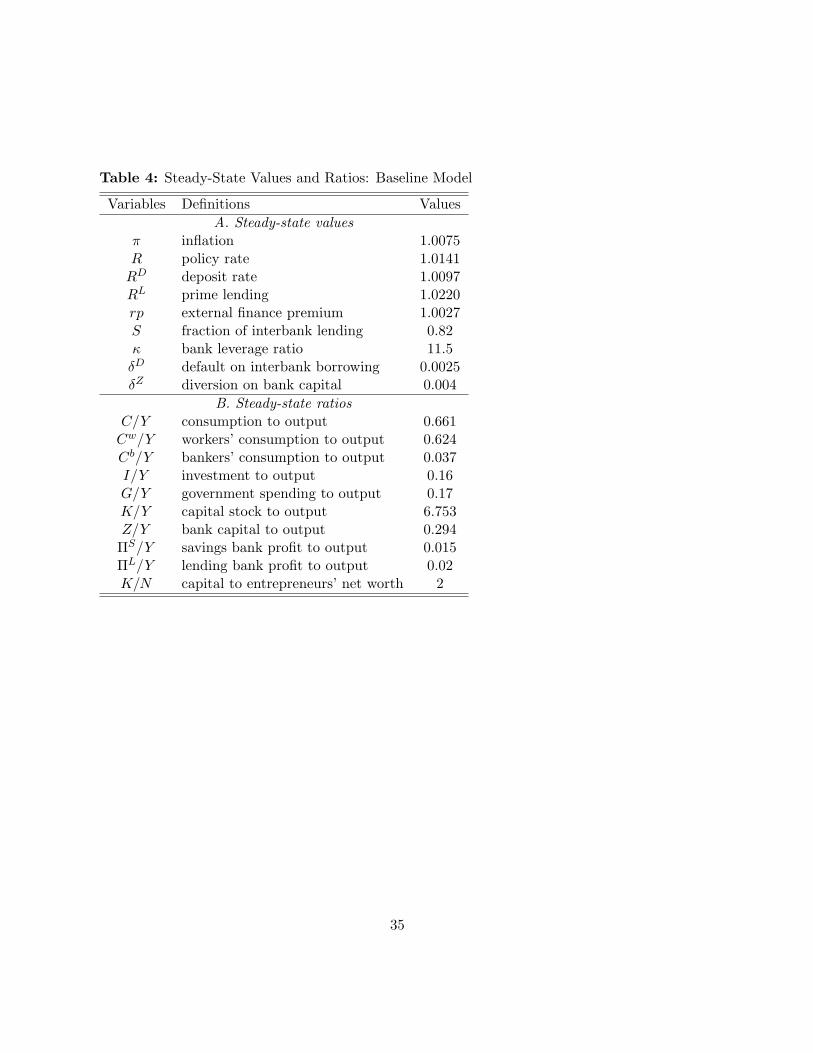
Table 4: Steady-State Values and Ratios: Baseline Model
Variables Definitions ValuesA. Steady-state values
π inflation 1.0075R policy rate 1.0141
RD deposit rate 1.0097RL prime lending 1.0220rp external finance premium 1.0027S fraction of interbank lending 0.82κ bank leverage ratio 11.5δD default on interbank borrowing 0.0025δZ diversion on bank capital 0.004
B. Steady-state ratiosC/Y consumption to output 0.661Cw/Y workers’ consumption to output 0.624Cb/Y bankers’ consumption to output 0.037I/Y investment to output 0.16G/Y government spending to output 0.17K/Y capital stock to output 6.753Z/Y bank capital to output 0.294ΠS/Y savings bank profit to output 0.015ΠL/Y lending bank profit to output 0.02K/N capital to entrepreneurs’ net worth 2
35
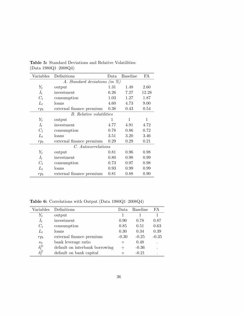
Table 5: Standard Deviations and Relative Volatilities:(Data 1980Q1–2008Q4)
Variables Definitions Data Baseline FAA. Standard deviations (in %)
Yt output 1.31 1.48 2.60It investment 6.26 7.27 12.28Ct consumption 1.03 1.27 1.87Lt loans 4.60 4.73 9.00rpt external finance premium 0.38 0.43 0.54
B. Relative volatilitiesYt output 1 1 1It investment 4.77 4.91 4.72Ct consumption 0.78 0.86 0.72Lt loans 3.51 3.20 3.46rpt external finance premium 0.29 0.29 0.21
C. AutocorrelationsYt output 0.81 0.96 0.98It investment 0.80 0.98 0.99Ct consumption 0.73 0.97 0.98Lt loans 0.93 0.99 0.99rpt external finance premium 0.81 0.88 0.90
Table 6: Correlations with Output (Data 1980Q1–2008Q4)
Variables Definitions Data Baseline FAYt output 1 1 1It investment 0.90 0.78 0.87Ct consumption 0.85 0.51 0.63Lt loans 0.30 0.34 0.39rpt external finance premium -0.30 -0.25 -0.35κt bank leverage ratio + 0.48 .δDt default on interbank borrowing + -0.36 .
δZt default on bank capital + -0.21 .
36
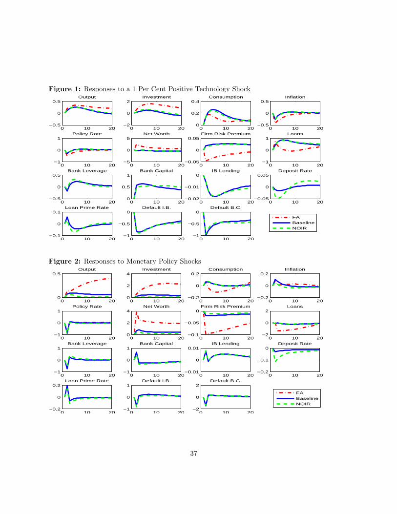
Figure 1: Responses to a 1 Per Cent Positive Technology Shock
0 10 20−0.5
0
0.5Output
0 10 20−2
0
2Investment
0 10 200
0.2
0.4Consumption
0 10 20−0.5
0
0.5Inflation
0 10 20−1
0
1Policy Rate
0 10 20−5
0
5Net Worth
0 10 20−0.05
0
0.05Firm Risk Premium
0 10 20−1
0
1Loans
0 10 20−0.5
0
0.5Bank Leverage
0 10 200
0.5
1Bank Capital
0 10 20−0.02
−0.01
0IB Lending
0 10 20−0.05
0
0.05Deposit Rate
0 10 20−0.1
0
0.1Loan Prime Rate
0 10 20−1
−0.5
0Default I.B.
0 10 20−1
−0.5
0Default B.C.
FABaselineNOIR
Figure 2: Responses to Monetary Policy Shocks
0 10 200
0.5Output
0 10 200
2
4Investment
0 10 20−0.2
0
0.2Consumption
0 10 20−0.2
0
0.2Inflation
0 10 20−1
0
1Policy Rate
0 10 200
2
4Net Worth
0 10 20−0.1
−0.05
0Firm Risk Premium
0 10 20−2
0
2Loans
0 10 20−1
0
1Bank Leverage
0 10 20−1
0
1Bank Capital
0 10 20−0.01
0
0.01IB Lending
0 10 20−0.2
−0.1
0Deposit Rate
0 10 20−0.2
0
0.2Loan Prime Rate
0 10 20−1
0
1Default I.B.
0 10 20−2
0
2Default B.C.
FABaselineNOIR
37
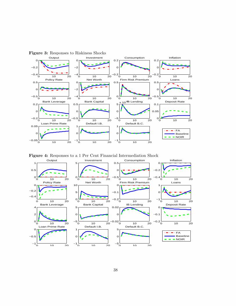
Figure 3: Responses to Riskiness Shocks
0 10 20−0.4
−0.2
0Output
0 10 20−4
−2
0Investment
0 10 20−0.2
0
0.2Consumption
0 10 20−0.2
0
0.2Inflation
0 10 20−0.5
0
0.5Policy Rate
0 10 20−4
−2
0Net Worth
0 10 200
0.5Firm Risk Premium
0 10 20−0.5
0
0.5Loans
0 10 20−0.2
0
0.2Bank Leverage
0 10 20−0.5
0
0.5Bank Capital
0 10 20−5
0
5x 10
−3IB Lending
0 10 200
0.05
0.1Deposit Rate
0 10 20−0.05
0
0.05Loan Prime Rate
0 10 20−1
0
1Default I.B.
0 10 20−1
0
1Default B.C.
FABaselineNOIR
Figure 4: Responses to a 1 Per Cent Financial Intermediation Shock
0 10 200
0.5
1Output
0 10 200
5Investment
0 10 20−0.5
0
0.5Consumption
0 10 20−0.4
−0.2
0Inflation
0 10 20
−0.4
−0.2
0Policy Rate
0 10 200
5
10Net Worth
0 10 20−0.2
−0.1
0Firm Risk Premium
0 10 20−1
0
1Loans
0 10 200
2
4Bank Leverage
0 10 20−5
0
5Bank Capital
0 10 20−0.02
0
0.02IB Lending
0 10 20−0.2
−0.1
0Deposit Rate
0 10 20−1
−0.5
0Loan Prime Rate
0 10 20−1
0
1Default I.B.
0 10 20−5
0
5Default B.C.
FABaselineNOIR
38
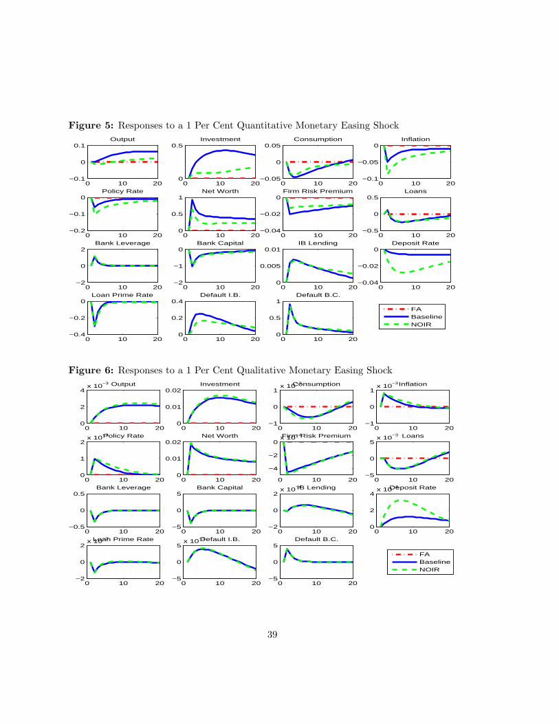
Figure 5: Responses to a 1 Per Cent Quantitative Monetary Easing Shock
0 10 20−0.1
0
0.1Output
0 10 200
0.5Investment
0 10 20−0.05
0
0.05Consumption
0 10 20−0.1
−0.05
0Inflation
0 10 20−0.2
−0.1
0Policy Rate
0 10 200
0.5
1Net Worth
0 10 20−0.04
−0.02
0Firm Risk Premium
0 10 20−0.5
0
0.5Loans
0 10 20−2
0
2Bank Leverage
0 10 20−2
−1
0Bank Capital
0 10 200
0.005
0.01IB Lending
0 10 20−0.04
−0.02
0Deposit Rate
0 10 20−0.4
−0.2
0Loan Prime Rate
0 10 200
0.2
0.4Default I.B.
0 10 200
0.5
1Default B.C.
FABaselineNOIR
Figure 6: Responses to a 1 Per Cent Qualitative Monetary Easing Shock
0 10 200
2
4x 10
−3 Output
0 10 200
0.01
0.02Investment
0 10 20−1
0
1x 10
−3Consumption
0 10 20−1
0
1x 10
−3Inflation
0 10 200
1
2x 10
−3Policy Rate
0 10 200
0.01
0.02Net Worth
0 10 20
−4
−2
0x 10
−4Firm Risk Premium
0 10 20−5
0
5x 10
−3 Loans
0 10 20−0.5
0
0.5Bank Leverage
0 10 20−5
0
5Bank Capital
0 10 20−2
0
2x 10
−4IB Lending
0 10 200
2
4x 10
−4Deposit Rate
0 10 20−2
0
2x 10
−3Loan Prime Rate
0 10 20−5
0
5x 10
−3Default I.B.
0 10 20−5
0
5Default B.C.
FABaselineNOIR
39
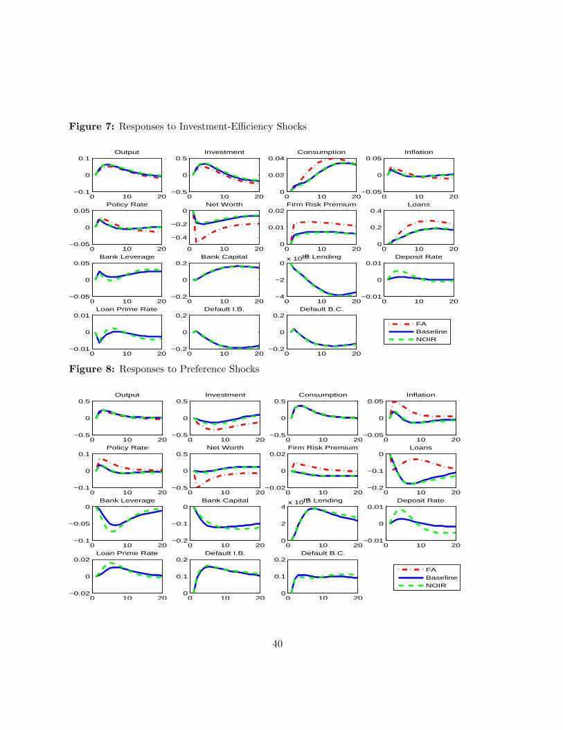
Figure 7: Responses to Investment-Efficiency Shocks
0 10 20−0.1
0
0.1Output
0 10 20−0.5
0
0.5Investment
0 10 200
0.02
0.04Consumption
0 10 20−0.05
0
0.05Inflation
0 10 20−0.05
0
0.05Policy Rate
0 10 20
−0.4
−0.2
0Net Worth
0 10 200
0.01
0.02Firm Risk Premium
0 10 200
0.2
0.4Loans
0 10 20−0.05
0
0.05Bank Leverage
0 10 20−0.2
0
0.2Bank Capital
0 10 20−4
−2
0x 10
−3IB Lending
0 10 20−0.01
0
0.01Deposit Rate
0 10 20−0.01
0
0.01Loan Prime Rate
0 10 20−0.2
0
0.2Default I.B.
0 10 20−0.2
0
0.2Default B.C.
FABaselineNOIR
Figure 8: Responses to Preference Shocks
0 10 20−0.5
0
0.5Output
0 10 20−0.5
0
0.5Investment
0 10 20−0.5
0
0.5Consumption
0 10 20−0.05
0
0.05Inflation
0 10 20−0.1
0
0.1Policy Rate
0 10 20−0.5
0
0.5Net Worth
0 10 20−0.02
0
0.02Firm Risk Premium
0 10 20−0.2
−0.1
0Loans
0 10 20−0.1
−0.05
0Bank Leverage
0 10 20−0.2
−0.1
0Bank Capital
0 10 200
2
4x 10
−3IB Lending
0 10 20−0.01
0
0.01Deposit Rate
0 10 20−0.02
0
0.02Loan Prime Rate
0 10 200
0.1
0.2Default I.B.
0 10 200
0.1
0.2Default B.C.
FABaselineNOIR
40
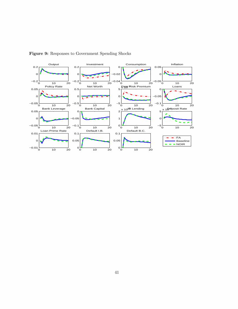
Figure 9: Responses to Government Spending Shocks
0 10 20−0.2
0
0.2Output
0 10 20−0.2
0
0.2Investment
0 10 20−0.04
−0.02
0Consumption
0 10 20−0.05
0
0.05Inflation
0 10 20−0.05
0
0.05Policy Rate
0 10 20−0.5
0
0.5Net Worth
0 10 20−5
0
5x 10
−3Firm Risk Premium
0 10 20−0.1
−0.05
0Loans
0 10 20−0.05
0
0.05Bank Leverage
0 10 20−0.1
−0.05
0Bank Capital
0 10 200
1
2x 10
−3IB Lending
0 10 20−5
0
5x 10
−3Deposit Rate
0 10 20−0.01
0
0.01Loan Prime Rate
0 10 200
0.05
0.1Default I.B.
0 10 200
0.05
0.1Default B.C.
FABaselineNOIR
41
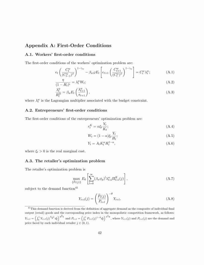
Appendix A: First-Order Conditions
A.1. Workers’ first-order conditions
The first-order conditions of the workers’ optimization problem are:
et
(Cw
t
(Cwt−1)
ϕ
)1−γw
− βwϕEt
[et+1
(Cw
t+1
(Cwt )ϕ
)1−γw]
= Cwt λw
t ; (A.1)
η
(1−Ht)ς= λw
t Wt; (A.2)
λwt
RDt
= βwEt
(λw
t+1
πt+1
), (A.3)
where λwt is the Lagrangian multiplier associated with the budget constraint.
A.2. Entrepreneurs’ first-order conditions
The first-order conditions of the entrepreneurs’ optimization problem are:
rKt = αξt
Yt
Kt; (A.4)
Wt = (1− α)ξtYt
Ht; (A.5)
Yt = AtKαt H1−α
t , (A.6)
where ξt > 0 is the real marginal cost.
A.3. The retailer’s optimization problem
The retailer’s optimization problem is
max{Pt(j)}
E0
[ ∞∑
l=0
(βwφp)lλwt+lΠ
Rt+l(j)
], (A.7)
subject to the demand function41
Yt+l(j) =
(Pt(j)Pt+l
)−θ
Yt+l, (A.8)
41This demand function is derived from the definition of aggregate demand as the composite of individual final
output (retail) goods and the corresponding price index in the monopolistic competition framework, as follows:
Yt+l =(∫ 1
0Yt+l(j)
θ−1θ dj
) θθ−1
and Pt+l =(∫ 1
0Pt+l(j)
1−θdj) 1
1−θ, where Yt+l(j) and Pt+l(j) are the demand and
price faced by each individual retailer j ∈ (0, 1).
42

where the retailer’s nominal profit function is
ΠRt+l(j) =
(πlPt(j)− Pt+lξt+l
)Yt+l(j)/Pt+l. (A.9)
The first-order condition for Pt(j) is
Pt(j) =θ
θ − 1Et
∑∞l=0(βwφp)lλw
t+lYt+l(j)ξt+l
Et∑∞
l=0(βwφp)lλwt+lYt+l(j)πl/Pt+l
. (A.10)
The aggregate price is
P 1−θt = φp(πPt−1)1−θ + (1− φp)P 1−θ
t . (A.11)
These lead to the following equation:
πt = βwEtπt+1 +(1− βwφp)(1− φp)
φpξt, (A.12)
where ξt is the real marginal cost, and variables with hats are log deviations from the steady-
state values (such as πt = log(πt/π)).
43

Appendix B: Data
1. Loans are measured by Commercial and Industrial Loans of all Commercial Banks (BUS-
LOANS), quarterly and seasonally adjusted;
2. The external finance premium is measured by the difference between Moody’s BAA cor-
porate bond yields and the 3-Month Treasury Bill (TB3MS);
3. Inflation is measured by quarterly changes in the GDP deflator (∆ log(GDPD));
4. The prime lending rate is measured by the Bank Prime Loan Rate (MPRIME);
5. The monetary policy rate is measured by the 3-Month Treasury Bill (TB3MS);
6. The deposit rate is measured by the weighted average of the rates received on the interest-
bearing assets included in M2 (M2OWN);
7. The real money stock is measured by the real M2 money stock per capita;
8. Output is measured by real GDP per capita;
9. Total Consumption is measured by Personal Consumption Expenditures (PCEC);
10. Investment is measured by Gross Private Domestic Investment (GPDI);
11. Government spending is measured by output minus consumption and investment (GDP
- PCEC- GPDI).
44