Bare-Bones R

A Brief Introductory Guide

Thomas P. HoganUniversity of Scranton

2010 All Rights Reserved

Citation and Usage

This set of PowerPoint slides is keyed to Bare-Bones R: A Brief Introductory Guide, by Thomas P. Hogan, SAGE Publications, 2010.

All are welcome to use and/or adapt the slides without seeking further permission but with the usual professional acknowledgment of source.

Part 1: Base R

1-1 What is R

A computer language, with orientation toward statistical applications

Relatively new

Growing rapidly in use

1-2 R’s Ups and Downs

Plusses Completely free, just download from Internet Many add-on packages for specialized uses Open source

Minuses Obscure terms, intimidating manuals,

odd symbols, inelegant output (except graphics)

1-3 Getting Started: Loading R

Have Internet connection Go to http://cran.r-project/ R for Windows screen, click “base” Find, click on download R Click Run, OK, or Next for all

screens End up with R icon on desktop

At http://cran.r-project.org/

Downloading Base R [Figs 1.1 – 1.4]

Click on Windows

Then in next screen, click on “base”

Then screens for Run, OK, or Next

And finally “Finish” will put R icon on desktop

What You Should Have when clicking on R icon:

Rgui and R Consoleending with R prompt (>) [Fig 1.5]

The R prompt (>)

> This is the “R prompt.”

It says R is ready to take your command.

1-4 Using R as Calculator

Enter these after the prompt,observe output

>2+3>2^3+(5)>6/2+(8+5)>2 ^ 3 + (5)

More as Calculator You can copy and paste, but don’t include the >

Use # at end of command for notes, e.g.

> (22+ 34+ 18+ 29+ 36)/5 #Calculating the average, aka mean

R as calculator: Not very useful

1-5 Creating a Data Set

> Scores = c(22, 34, 18, 29, 36)c means “concatenate” in R

– in plain English “treat as data set”

Now do:>Scores

R will print the data set

Important Rules

1. We created a variable2. Variable names are case sensitive3. No blanks in name

(can use _ or . to join words, but not -)

4. Start with a letter (cap or lc)5. Can use <- instead of =

Another variable Create SCORES, using <-

> SCORES<-c(122, 134, 118, 129, 124)

NB: SCORES different than ScoresCheck with>SCORES>Scores

Non-numeric Data

Enclose in quotes, single or double Separate entries with comma Example:

> names = c(“Mary”, “Tom”, “Ed”, “Dan”,

“Meg”)

Saving Stuff To exit: either X or quit ( ) Brings up this screen:

Do what you want: Yes or No Do Yes, then re-open R, get Scores & names

Special Note on Saving

Previous slide assumes you control

computer

If not, use File, Save Workspace, name

file, click Save

Works much like saving a file in Microsoft

To retrieve, do File, Load Workspace, find

file, click Open

1-6 Using R Functions: Simple Stuff

Commands for mean, sd, summary(NB: function names case sensitive)

mean(Scores) sd(Scores) summary(Scores)

Command for correlation cor(Scores,SCORES)

R functions

A zillion of ‘em R’s big strength, most common

use For examples:

Help R functions(text) Enter name of a function (e.g., sd)

Yields lots (!) of information

1-7 Reading in Larger Data Sets

In Excel, enter (or download) the SATGPA20 file

Save as .xls

Then save as Text (tab delimited) file Will have .txt extension

… Larger Data SetsThe read.table command

Now read into R like this:

>SATGPA20R=read.table("E:/R/SATGPA20.txt", header =T)

Need exact path, in quotes

header = T T or TRUE, F or FALSE Depends on opening line of file

The file.choose ( ) command

At > enter file.choose ( ) Accesses your system’s files, much

like Open in Microsoft Find the file, click on it R prints the exact path in R

Console Can copy and paste into read.table

Checking what you’ve got:

Enter>SATGPA20R Then>mean (SATGPA20R) Try>mean (GPA)

The attach Command

To access individual variables, do this:

>attach(SATGPA20R)

Now try:>mean(GPA)

The data.frame Command

Let’s create these 3 variables with c> IQ = c(110, 95, 140, 89, 102)> CS = c(59, 40, 62, 40, 55)> WQ = c(2, 4, 5, 1, 3)

Then put them together with:>All_Data = data.frame(IQ, CS, WQ) Check with:>mean(All_Data)

1-8 Getting Help

>help(sd) >example(sd) On R Console:

Help

R functions (text)Enter function name, click OK

Reminder: function names case sensitive

R’s “function” terms

R language: function(arguments)

Plain English: Do this (to this)

or Do this (to this, with these conditions)

1-9 Dealing with Missing Data

NB: It’s a pain in R!

Key items In data, enter NA for a missing value In (most) commands, use na.rm=T

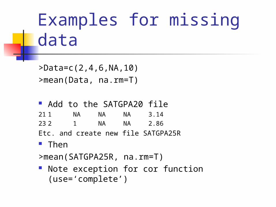
Examples for missing data

>Data=c(2,4,6,NA,10)>mean(Data, na.rm=T)

Add to the SATGPA20 file21 1 NA NA NA 3.1423 2 1 NA NA 2.86

Etc. and create new file SATGPA25R Then>mean(SATGPA25R, na.rm=T) Note exception for cor function (use=‘complete’)

1-10 Using R Functions: Hypothesis tests

Be sure you have an active data set (SATGPA25R), using attach if needed

Then, to test male vs. female on SATM:>t.test(SATM~SEX) # note tilde~

Examples of changing defaults:>t.test(SATM~SEX, var.equal=TRUE,

conf.level=0.99)

Hypothesis tests: Chi-square

Using SEX and State variables in SATGPA25R

chisq.test (SEX, State)

1-11 R Functions for Commonly Used Statistics

function calculates thismean ( ) meanmedian ( ) medianmode ( ) modesd ( ) standard deviationrange ( ) rangeIQR ( ) interquartile rangemin ( ) minimum valuemax ( ) maximum valuecor ( ) correlationquantile ( ) percentilet.test ( ) t-testchisq.test ( ) chi-sqaure

NB1: See notes in text for detailsNB2: R contains many more functions

1-12 Two Commands for Managing Your Files

> ls ( )Will list your currently saved files

> rm (file)Insert file name; this will remove the

file

NB: R has many such commands

1-13 R Graphics R graphs: good, simple Let’s start with hist and boxplot

with the SATGPA25R file>hist(SATM) >boxplot(SATM)

>boxplot(SATV, SATM) R Graphics window opens,

need to minimize to get R Console

More Graphics: plot

Create these variables>RS=c(12,14,16,18,25)>MS=c(10,8,16,12,20)

Now do this:>plot(RS, MS)

Line of Best Fit

Do these for the RS and MS variables:

> lm(MS~RS) # lm means linear model

> res=lm(MS~RS) # res means residuals

> abline(res) # read as ‘a-b’ line

Controlling Your Graphics: A Brief Look

R has many (often obscure) ways for controlling graphics; we’ll look at a few

Basically, we’ll change “defaults”

Examples (try each one): Limits (ranges) for X and Y axes>plot(RS, MS, xlim = c(5,25), ylim = c(5,25))

Controlling Graphs: More Examples

Plot characters:>plot(RS, MS, pch=3)

Line widths>plot(RS, MS, pch=3, lwd=5)

Axis labels>plot(RS, MS, xlab = “Reading Score”, ylab = “Math Score”)

You can put them all together in one command

Part 2: R Commander

2-1 What is R Commander? Point and click version of R Uses (and prints) base R commands

Loading: Easy – it’s just a package See next slide

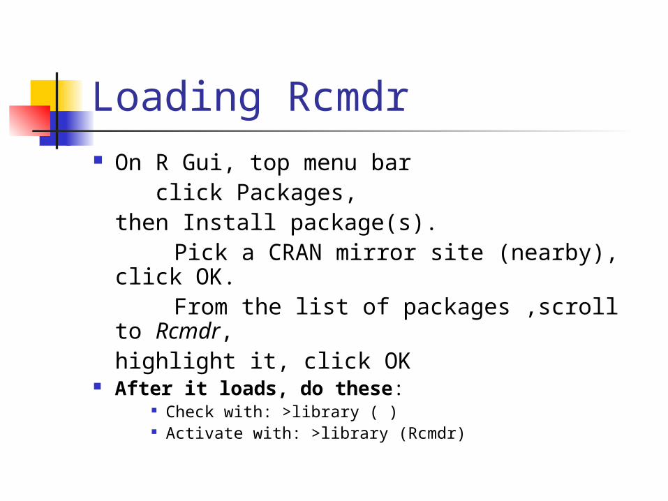
Loading Rcmdr On R Gui, top menu bar

click Packages, then Install package(s).

Pick a CRAN mirror site (nearby), click OK. From the list of packages ,scroll to Rcmdr,

highlight it, click OK After it loads, do these:

Check with: >library ( ) Activate with: >library (Rcmdr)

Rcmdr’s extra packages Scary message when first activating

Rcmdr:

Just click Yes – and take a break

The R Commander Window You get, R Commander window with

Script window

Output window (incl Submit button)

Message window

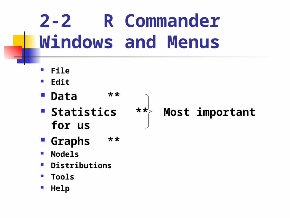
2-2 R Commander Windows and Menus File Edit

Data ** Statistics ** Most important

for us Graphs ** Models Distributions Tools Help

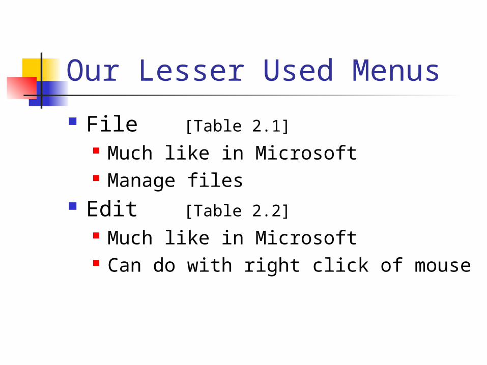
Our Lesser Used Menus

File [Table 2.1] Much like in Microsoft Manage files

Edit [Table 2.2] Much like in Microsoft Can do with right click of mouse

Our Lesser Used Menus (cont) Models

Mostly more advanced stats Distributions

Tools Load packages Options – change output defaults

Help Searchable index R Commander manual

2-3 The Data Menu (very important)

(Submenus for creating/getting data sets)

New data set – create new data set

Load data set – only for existing .rda data

Import data – import from various file types

Data in packages – not important for us

Data Menu (cont.)(Submenus for managing data

sets)

Active data set Do stuff with current data set

Manage variables in active data set Do stuff with variables in current data

set

New data set [Fig. 2.3]

Click on it, brings up spreadsheet

Name it SampleData

New data set (cont) Enter these data:var1 var2 var32 1 55 4 73 7 86 8 99 2 9 Then kill window with X Note: SampleData in Active Data Set

Now Try These View active data set Edit active data set In Script window, type*

mean(SampleData) sd (SampleData) mean(var1) [gives error message] Attach(SampleData) mean(var1)

* When typing do not include >, do hit Submit

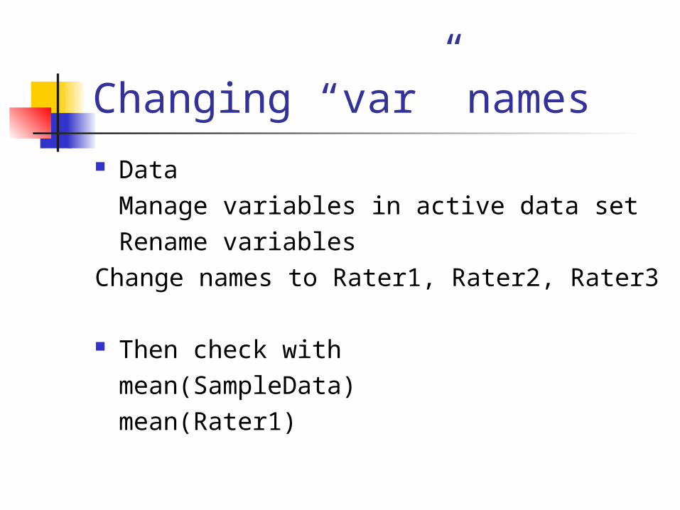
Changing “var” names Data

Manage variables in active data setRename variables

Change names to Rater1, Rater2, Rater3

Then check withmean(SampleData)mean(Rater1)

Compute new variable Data

Manage variables in active data set Compute new variable

Give name to new variable, call it Total In ‘Expression to compute’, enter

Rater1+Rater2+Rater3 Check with

View data set mean (SampleData)

Import data(very important submenu)

Allows importing from .txt file SPSS file Excel file Several others

Try it with a .txt file (must already exist; try with SATGPA25.txt)

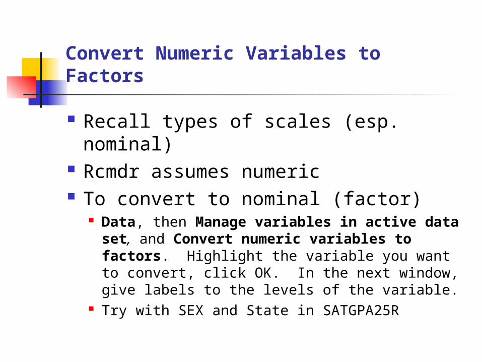
Convert Numeric Variables to Factors

Recall types of scales (esp. nominal) Rcmdr assumes numeric To convert to nominal (factor)

Data, then Manage variables in active data set, and Convert numeric variables to factors. Highlight the variable you want to convert, click OK. In the next window, give labels to the levels of the variable.

Try with SEX and State in SATGPA25R

2-4 The Statistics Menu

Obviously very important Most pretty clear how to do

Some go beyond intro stats Some surprises on what’s where

We’ll just sample some of them Put SATGPA25R in Active data set

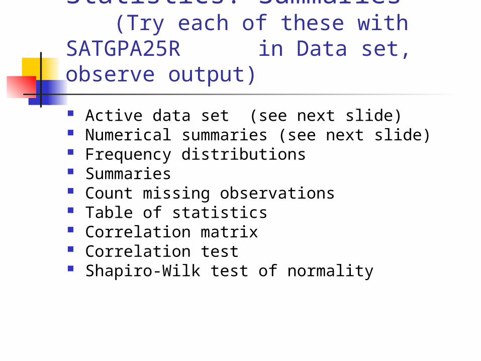
Statistics: Summaries(Try each of these with

SATGPA25R in Data set, observe output)

Active data set (see next slide) Numerical summaries (see next slide) Frequency distributions Summaries Count missing observations Table of statistics Correlation matrix Correlation test Shapiro-Wilk test of normality

Getting started on Stat menu

Statistics – Summaries - Active data set

Statistics – Summaries – Numerical summaries

Etc. with others

Numerical Summaries Screen [Fig 2.4]

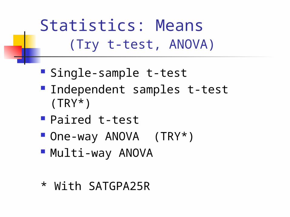
Statistics: Means(Try t-test, ANOVA)

Single-sample t-test Independent samples t-test (TRY*) Paired t-test One-way ANOVA (TRY*) Multi-way ANOVA

* With SATGPA25R

Independent Samples t-test(Do SATM by SEX) [Fig 2.7]

One-Way ANOVA

(Do GPA by State) [Fig 2.8]

Two-Way Table (chi-square) [Fig 2.9]

Statistics - Contingency tables - Two-Way table

2-5 The Graphics Menu

All pretty intuitive (if you know the graph)

Try with SATGPA25R Pie: State Histogram: SATM Boxplot by group: SATM by SEX Scatterplot: GPA from SATV

Changing Graphs Appearance

Rcmdr Graphs uses defaults

Change them in Script window

Use commands given earlier

Many ways to do; not terribly intuitive

See example on next slide

Changing Graphs Defaults: Example

Histogram of GPA (with defaults):

Hist(SATGPA25R$GPA, scale="frequency", breaks="Sturges", col="darkgray")

[copy, paste, change, Submit]Hist(SATGPA25R$GPA, scale="frequency",

breaks=4, col="black", lwd=3)

2-6 The Distributions Menu: Two Quick Examples

Distributions Continuous distributions Normal distribution

Normal probabilities [insert -1.5] Distributions

Continuous distributions t distribution

t probabilities [insert 1.71, df 28]

Part 3: Some Other Stuff

Supplementary, Not Essential, Brief

3-1 A Few Other Ways to Enter Data 3-2 Exporting R Results 3-3 Bonus: Build Your Own Functions 3-4 An Example of an Add-on Package 3-5 Keeping Up to Date 3-6 Going Further: Selected References

3-1 A Few Other Ways to Enter Data

From Word, a few rules1. One space between entries2. NA for missing data3. Save as Plain text (.txt)4. Access with read.table

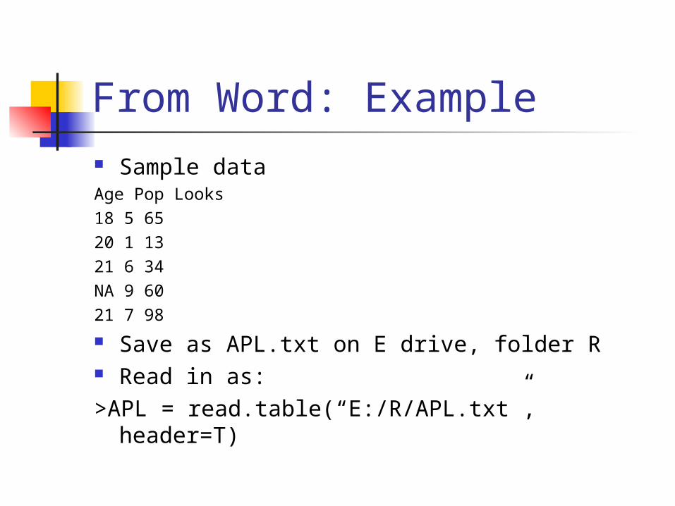
From Word: Example Sample dataAge Pop Looks18 5 6520 1 1321 6 34NA 9 6021 7 98

Save as APL.txt on E drive, folder R Read in as:>APL = read.table(“E:/R/APL.txt”, header=T)

Checking from Word

Do these: >APL >mean (APL) >mean (Pop) [gives error] >attach (APL) >mean (Pop)

From SPSS file Be sure you have foreign library

Check with: > library ( ) [if needed, load] Activate with: > library (foreign)

Have an SPSS file FinalData, which we’ll put into FinalR, using read.spss andto.data.frame like this

>FinalR = read.spss(‘E/Project/FinalData.sav’, to.data.frame = T)

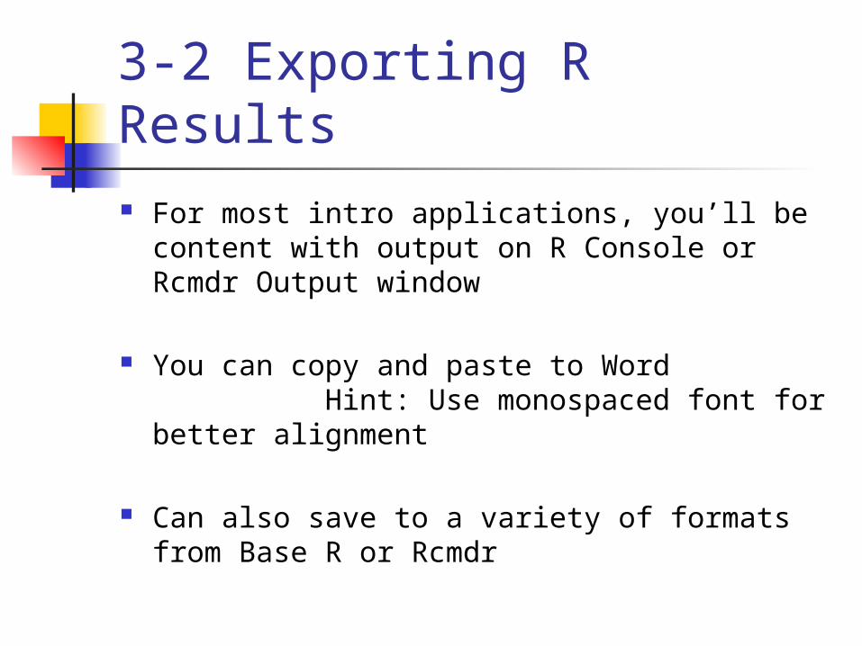
3-2 Exporting R Results For most intro applications, you’ll be content

with output on R Console or Rcmdr Output window

You can copy and paste to Word Hint: Use monospaced font for better

alignment

Can also save to a variety of formats from Base R or Rcmdr

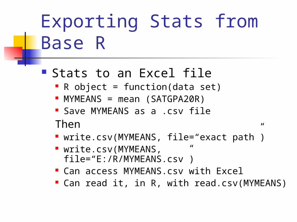
Exporting Stats from Base R Stats to an Excel file

R object = function(data set) MYMEANS = mean (SATGPA20R) Save MYMEANS as a .csv file

Then write.csv(MYMEANS, file=“exact path”) write.csv(MYMEANS,

file=“E:/R/MYMEANS.csv”) Can access MYMEANS.csv with Excel Can read it, in R, with read.csv(MYMEANS)

Exporting Graphs from Base R

Easy in R Graphics window and works same for base R and

Rcmdr Right click on the graph Copy as metafile (and paste

wherever) Save as metafile (and save

wherever)

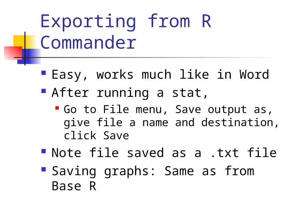
Exporting from R Commander

Easy, works much like in Word After running a stat,

Go to File menu, Save output as, give file a name and destination, click Save

Note file saved as a .txt file Saving graphs: Same as from Base

R

3-3 Bonus: Build Your Own Functions You can custom-make a function

and save it for future use Example: function to get mean of a

data set + 2 times its SD> weirdstat = function(x) mean(x) +

(2*sd(x)) Now try:

>weirdstat(GPA) Function names get saved like data

sets and they are case sensitive

3-4 An Example of an Add-on Package

Getting Info about Packages (need Internet) Take it slowly Go to Task Views in

http://cran.r-project.org/ Gives categories of packages (23 now) Click on link for a category Package names: usually cryptic, often

obscure To see what’s in a package:

Click on its link Look at its Reference Manual

Installing an Add-on Package Follow usual steps for download

Be sure to activate with >library(pkg) Download psychometric package

Using an Add-on Package Basically a collection of functions

Examples with psychometric package r.nil(r, n) rdif.nul(r1, r2, n1, n2)

3-5 Keeping Up to Date

All parts of R (base, Commander, add-on packages) periodically updated

Check cran-r site for updates

Update by downloading new version(need Internet connection for this)

3-6 Selected References

Key URLs R home: http://www.r-project.org/ Download: http://cran.r-project.org/ For many other introductions to R:

http://cran.r-project.org/other-docs.html

References (cont)

Some ‘Official’ books – online as pdfs

Fox, J. (2005). Getting started with the R Commander

R Development Core Team (2009). R Data Import/Export version 2.9.0.

Venables, W. N., Smith, D. M., & the R Development Core Team (2009). An introduction to R. Notes on R: A programming environment for data analysis and graphics version 2.9.0.

References (cont)

Some other books Dalgaard, P. (2008). Introductory statistics with R

(2nd ed.). New York: Springer.

Everitt, B. S., & Hothorn, T. (2006). A handbook of statistical analyses using R. Boca Raton, FL: Chapman and Hall.

Murrell, P. (2005). R graphics. Boca Raton, FL: Chapman and Hall.

To cite use of R To cite the use of R for statistical work,

R documentation recommends the following:

R Development Core Team (2009). R: A language and environment for statistical computing. R Foundation for Statistical Computing, Vienna, Austria. ISBN 3-900051-07-0, URL http://www.R-project.org.

Get the latest citation by typing citation ( ) at the > prompt in the R Console.

The End