Embed Size (px)
Citation preview
Str
uct
ure
s R
ese
arc
h
Rep
ort
20
02
/7
83
Un
ivers
ity o
f Flo
rid
a
C
ivil
an
d C
oast
al
En
gin
eeri
ng
University of FloridaCivil and Coastal Engineering
Final Report January 2002
Barge Impact Testing of the St. George Island Causeway BridgePhase I : Feasibility Study Principal investigators:
Gary R. Consolazio, Ph.D. Ronald A. Cook, Ph.D., P.E. Graduate research assistant:
G. Benjamin Lehr Department of Civil and Coastal Engineering University of Florida P.O. Box 116580 Gainesville, Florida 32611 Sponsor: Florida Department of Transportation (FDOT) Henry T. Bollmann, P.E. – Project manager Contract: UF Project No. 4504-783-12 FDOT Contract No. BC-354 RPWO 23

Technical Report Documentation Page
1. Report No. 2. Government Accession No.
3. Recipient's Catalog No.
BC354 RPWO #23
4. Title and Subtitle
5. Report Date January 2002
6. Performing Organization Code
Barge Impact Testing of the St. George Island Causeway Bridge
8. Performing Organization Report No. 7. Author(s) G. R. Consolazio, R. A. Cook, and G. B. Lehr
4910 45 04 783
9. Performing Organization Name and Address
10. Work Unit No. (TRAIS)
11. Contract or Grant No. BC354 RPWO #23
University of Florida Department of Civil & Coastal Engineering P.O. Box 116580 Gainesville, FL 32611-6580
13. Type of Report and Period Covered 12. Sponsoring Agency Name and Address
Final Report
14. Sponsoring Agency Code
Florida Department of Transportation Research Management Center 605 Suwannee Street, MS 30 Tallahassee, FL 32301-8064
15. Supplementary Notes
16. Abstract
The purpose of this research project was to determine the feasibility of conducting full-scale experimental barge impact testing of the SR 300 / Saint George Island Causeway bridge in Apalachicola, Florida and to establish the parameters of the proposed testing program. The aspects of feasibility that were investigated included: environmental, geographical, and scheduling feasibilities. Experimental design and applicability analyses were carried out through the use of dynamic finite element impact simulation using the LS-DYNA code. Results from the study indicated that the proposed impact testing program is feasible with respect to all areas investigated. Specific results from the feasibility study included the identification of an overall time window for the full-scale testing, testing location, and a preliminary testing program. Finite element impact simulations were conducted for a range of impact scenarios in order to select optimal parameters for the experimental test program. Dynamic impact simulations resulted in the selection of a barge cargo weight and a set of impact velocities for use in the full-scale testing program. In addition, barge loads predicted by dynamic impact simulation were compared to the AASHTO equivalent static load method and to finite element simulations of static barge crush tests.
17. Key Words 18. Distribution Statement
Vessel impact load, barge impact, bride pier, finite element modeling, soil-structure interaction
No restrictions. This document is available to the public through the National Technical Information Service, Springfield, VA, 22161
19. Security Classif. (of this report)
20. Security Classif. (of this page) 21. No. of Pages
22. Price
Unclassified Unclassified 128
Form DOT F 1700.7 (8-72) Reproduction of completed page authorized

Barge Impact Testing of the St. George Island Causeway Bridge
Phase I : Feasibility Study
Contract No. BC-354 RPWO#23 UF Project No. 4910-4504-783-12
Principal Investigators : Gary R. Consolazio, Ph.D. Ronald A. Cook, Ph.D., P.E. Graduate Research Assistant: G. Benjamin Lehr FDOT Technical Coordinator: Henry T. Bollmann, P.E.
Engineering and Industrial Experiment Station Department of Civil & Coastal Engineering
University of Florida Gainesville, Florida
i
TABLE OF CONTENTS
CHAPTER 1 : INTRODUCTION
1.1 Overview ................................................................................................................................... 1 1.2 Objectives.................................................................................................................................. 2 1.3 Scope of Work........................................................................................................................... 3
CHAPTER 2 : PROCEDURES FOR DETERMINING BARGE IMPACT LOADS
2.1 Introduction ............................................................................................................................... 6 2.2 Design of bridge structures for vessel impact ........................................................................... 7
2.2.1 Current impact resistance systems ................................................................................... 8 2.3 AASHTO specifications............................................................................................................ 8
2.3.1 Permissible methods of analysis ...................................................................................... 8 2.3.2 Kinetic energy method ..................................................................................................... 9 2.3.3 Experimental basis for AASHTO barge impact force equations ................................... 11
2.4 Previous experimental impact tests ......................................................................................... 12
CHAPTER 3 : PROPOSED TEST PROGRAM AND IDENTIFICATION OF FEASIBILITY ISSUES
3.1 Overview of proposed experimental testing............................................................................ 16 3.1.1 Instrumentation for measurement of impact loads............................................................... 19
3.1.2 Proposed schedule for full scale impact experiments .................................................... 21 3.2 Issues affecting feasibility of proposed test program.............................................................. 23
CHAPTER 4: ENVIRONMENTAL PERMITTING
4.1 Introduction ............................................................................................................................. 25 4.2 Oyster Beds ............................................................................................................................. 25 4.3 Manatees and Protected Bird Estuaries................................................................................... 27 4.4 Noise Levels Associated with Impact Testing ........................................................................ 27 4.5 Falling Debris Containment .................................................................................................... 28 4.6 Proposed Permit Acquisition Process ..................................................................................... 29
CHAPTER 5 : IDENTIFICATION, ACQUISITION, AND OPERATION OF BARGE
5.1 Selection of Test Barge ........................................................................................................... 30 5.1.1 Special considerations for use of aging barges .............................................................. 33
5.2 Estimated Barge Acquisition Costs......................................................................................... 33 5.3 Tug Requirements for Conducting the Test Program ............................................................. 34
CHAPTER 6 : GEOGRAPHICAL ISSUES
6.1 Introduction ............................................................................................................................. 36 6.2 Bathymetric Survey Results .................................................................................................... 37
ii
CHAPTER 7 : SCHEDULING
7.1 General Scheduling Requirements .......................................................................................... 40 7.2 Coordination with demolition schedule .................................................................................. 41
CHAPTER 8 : ESTABLISHING IMPACT TESTING CONDITIONS
8.1 Basis for selecting impact conditions...................................................................................... 43 8.2 Finite element impact simulation ............................................................................................ 44 8.3 Future use of barge and pier finite element models ................................................................ 45 Chapter 9 : Development of a barge finite element model 9.1 Structural description of typical jumbo hopper barge............................................................. 47 9.2 General model characteristics and considerations .................................................................. 49 9.3 Zone one – Impact zone of barge ............................................................................................ 50
9.3.1 Geometry and boundary considerations......................................................................... 50 9.3.2 Material Properties ......................................................................................................... 53 9.3.3 Selection of contact entities and algorithms................................................................... 55 9.3.4 Conflicts with combining contact algorithms ................................................................ 55
9.4 Zone two – frame modeled bow portion ................................................................................. 58 9.4.1 Geometry and boundary considerations......................................................................... 58 9.4.2 Material Properties ......................................................................................................... 61
9.5 Zone three – Rear Hopper ....................................................................................................... 62 9.5.1 Geometry and boundary considerations......................................................................... 62 9.5.2 Material Properties ......................................................................................................... 63 9.5.3 Determination of barge weight....................................................................................... 63
9.6 Modeling buoyancy and gravity.............................................................................................. 64 9.6.1 Geometric setup of buoyancy springs ............................................................................ 65 9.6.2 Boundary constraints of buoyancy springs .................................................................... 65 9.6.3 Determination of spring offsets for buoyancy springs ................................................... 67
CHAPTER 10 : DEVELOPMENT OF FINITE ELEMENT MODELS FOR CAUSEWAY PIERS
10.1 Description of causeway support piers.................................................................................. 70 10.2 General model characteristics and considerations ................................................................ 71 10.3 Finite element model of pier-1 .............................................................................................. 72
10.3.1 Geometry and boundary considerations....................................................................... 72 10.3.2 Material properties ....................................................................................................... 75 10.3.3 Soil-pile interaction model ........................................................................................... 76
10.4 Finite element model of pier-3 .............................................................................................. 87 10.4.1 Geometry and boundary consideration ........................................................................ 87 10.4.2 Material Properties ....................................................................................................... 89 10.4.3 Soil-pile interaction model ........................................................................................... 90

iii
CHAPTER 11 : DETERMINATION OF IMPACT CONDITIONS USING FINITE ELEMENT SIMULATION
11.1 Introduction ........................................................................................................................... 94 11.2 Simulation of barge impacts using merged barge and pier finite element models .............. 95
11.2.1 Contact definition for determining and recording impact force history....................... 95 11.2.2 Alignment of barge and pier models ............................................................................ 96
11.3 Results for pier-1 impact simulations ................................................................................... 97 11.4 Results for pier-3 impact simulations ................................................................................... 99 11.5 Evaluation of safety using FB-PIER analyses..................................................................... 102 11.6 Comparison of AASHTO loads, dynamic impact loads, and static crush loads................. 103 11.7 Impact velocities for full scale testing................................................................................. 110
CHAPTER 12 : CONCLUSIONS
12.1 Assessment of feasibility for full-scale barge impact test program .................................... 112
REFERENCES............................................................................................................................ 114
APPENDIX : BARGE IMPACT FORCE CALCULATIONS .................................................. 116
1
CHAPTER 1 INTRODUCTION
1.1 Overview
In the design and evaluation of bridge structures that cross navigable waterways,
the loads imparted to a bridge during potential ship and barge impact events must be
carefully considered. While bridge design documents such as the AASHTO Guide
Specification and Commentary for Vessel Collision Design of Highway Bridges
(AASHTO 1991) address these issues with code-based loading conditions, very little
actual impact test data has ever been recorded for such events. Given the large number of
bridges in Florida that cross navigable waterways, FDOT has a need for reliable and
accurate barge impact-loading data for use in bridge design, retrofit, and evaluation. In
this context, the term “accurate” is taken to indicate that the lateral impact loads used for
design are not unconservative, but are also not so overly conservative that they result in
needlessly expensive bridge designs.
The replacement of the St. George Island causeway bridge near Apalachicola,
Florida with a new bridge structure represents a unique and valuable opportunity to
experimentally measure barge impact forces directly. After opening the new bridge to
traffic, the older structure will be impacted by a hopper barge and the lateral forces
imparted to the bridge piers will be directly measured. Data collected from the tests will
be used to improve the accuracy of the barge impact loading models used in Florida,
nationally, and possibly internationally. If impact loads measured during the proposed
testing indicate that the AASHTO specifications predict unconservatively small loads,
then a greater level of safety may be achieved by updating the specifications to

2
incorporate the test data collected. However, if the specifications predict loads that are
shown to be overly conservative, then modifications could be made to reduce the design
loads associated with barge impact events. This in turn would lead to a cost benefit for
FDOT and other agencies in terms of reducing the required size of bridge pier
substructures.
1.2 Objectives
Conducting full scale barge impact testing on the St. George Island causeway
bridge represents a large-scale and multifaceted endeavor requiring substantial advance
planning. As such, it was decided that the overall program should be broken down into
several distinct phases. Phase I consists of a feasibility study that examines a wide variety
of issues relating to the successful completion of the proposed testing. Phase II consists
primarily of designing large scale instrumentation systems and Phase III consists of
conducting the actual barge impact tests and interpreting the data collected.
The Phase I feasibility study has been completed and this report documents the
results of that study in detail. The overriding objective of this study was to determine
whether or not the proposed testing program can be successfully carried out without
encountering insurmountable hindrances. Potential barriers to successful completion of
the testing included issues of environmental permitting, schedule coordination with the
contractor, geographic issues, safety considerations, and many more. In addition,
numerous testing aspects relating specifically to the barge were studied. These included
determining barge impact velocities, angles, acceleration paths, and payload conditions
for the test program; predicting barge and bridge damage levels to ensure safety; and

3
determining test conditions that would result in impact forces representative of realistic
barge impact events.
1.3 Scope of Work
In order to achieve the objectives listed above, a number of different tasks were
included in the scope of work for the Phase I feasibility study. Each of these tasks are
identified below.
• Review current impact load determination methods (Chapter 2)
Conduct a review of the current AASHTO barge impact provisions.
• Conduct a literature search (Chapter 2)
Conduct a literature search for any published papers describing previously carried
out experimental barge impact testing programs.
• Identify feasibility issues and outline proposed testing program (Chapter 3)
Generate a list of areas to be studied in order to determine whether or not the
proposed testing is feasible. Outline a testing program that maximizes the
usefulness of the data collected while also maximizing the probability of success
with respect to permitting, scheduling, costs, and other contributing factors.
• Study environmental permitting issues (Chapter 4)
Review pertinent environmental permitting issues including oyster beds,
manatees, protected bird estuaries, noise restrictions, and water turbidity
restrictions. This task also included discussions with the contractor that is building
the new bridge, and a review of the contractor’s environmental permitting
documents.

4
• Investigate barge type, size, cost, and navigation requirements (Chapter 5)
Select most appropriate type and size of barge, obtain cost estimates for new and
used barges, estimate time required for barge acquisition, and determine tug
requirements for navigating the test barge during impact testing.
• Consider geographical issues (Chapter 6)
Review water depth data for area near the existing and new bridge structures,
conduct an onsite bathymetric survey to directly evaluate water depths, and
determine most appropriate barge acceleration paths considering new bridge
location, water depth data, and presence of other features such as oyster beds,
power lines, etc.
• Consider scheduling and time windows (Chapter 7)
Develop a schedule for the full scale testing and examine the sensitivity of the
schedule to unforeseen delays. Meet with the contractor handling the demolition
of the existing structure to determine the feasibility of performing the testing
without interfering with the overall bridge replacement process.
• Develop finite element models for impact simulation (Chapters 8, 9, 10)
Develop finite element models of a hopper barge and of selected piers in existing
St. George Island causeway bridge structure using construction plans and
available soil data. Pier models include the pier structure, pile cap, piles, and soil
springs.
• Establish impact conditions, estimate response, ensure safety (Chapters 11)
Using the barge and pier finite element models, conduct numerous simulated

5
impact scenarios. The goal is to choose a barge size and cargo mass that
maximizes the variety of impact loads that can be imparted to the bridge while
still ensuring safety. Simulations are conducted at various impact velocities, on
various piers, and with different barge masses to determine the time-history of
lateral force imparted to the bridge piers. This information is then used to
determine the anticipated level of damage that will occur in the barge and to
determine the margin of safety against failure of the pier structures tested. Finally,
these models will be used in subsequent phases of the project to design and
develop instrumentation systems for measuring the impact loads.
In the chapters that follow, each of the tasks outlined above is discussed in further detail
along with results generated and conclusions drawn.

6
CHAPTER 2 PROCEDURES FOR DETERMINING
BARGE IMPACT LOADS
2.1 Introduction
Vessel impact is one of the most significant design considerations for bridges that
span navigable waterways. Of these bridges, the most vulnerable for vessel collision are
those that span coastal or inland waterways (Larsen 1993). In fact, until just twenty-five
years ago, vessel impact loading was not even a consideration when designing bridges.
Vessel impacts often result in costly bridge repairs and in some cases, loss of lives.
Probably the most noted incident is the 1980 collapse of the Sunshine Skyway Bridge in
Tampa, Florida. The cargo ship, Summit Venture collided with one of the anchor piers of
the bridge causing the collapse of almost 1300 feet of bridge deck and the loss of thirty-
five lives (AASHTO 1991, Larsen 1993). A fatal barge impact event occurred in 1993
near Mobile, Alabama when a barge tow collided with a CSX railroad bridge over Bayou
Canot resulting in a large lateral displacement of the structure. Minutes later a fully
loaded Amtrak train attempted to cross the bridge. The weight of the fully loaded train on
the damaged structure was enough to cause a collapse, which resulted in forty-seven
fatalities (Knott 2000). Most Recently, in September 2001, a barge tow collided with the
Queen Isabella causeway, the longest bridge in Texas, destroying three spans and killing
five people. In addition to the fatalities, this collapse left over one thousand residents and
hundreds of tourists stranded on South Padre island. These are just a few examples of
what can occur when vessels, such as ships and barges, collide with bridge structure. In
fact, many vessel impacts occur world wide with at least one serious collision each year
on average (Larsen 1993).

7
2.2 Design of bridge structures for vessel impact
As a result of the rise in incident rate of vessel collisions with bridge structures, a
pooled fund research program sponsored by eleven states and the FHWA was initiated in
1998 to investigate methods of safeguarding bridges against collapse when impacted by
ships or barges. The findings from the research were adopted by AASHTO and are
presented in the Guide Specification and Commentary for Vessel Collision Design of
Highway Bridges (AASHTO 1991). The guide specification is the basis for bridge design
with respect to the resistance of loads resulting from vessel collision. The specification
allows for two types of bridge resistance design. AASHTO allows the designer to either
design the bridge pier to withstand the vessel impact loads alone or to design a secondary
pier protection system that will absorb the vessel impact loads and prevent the bridge
structure itself from being impacted. In addition to these design standards, the AASHTO
vessel impact specification recommends methodologies for placement of the bridge
structure as well as specifications for navigational aids. Both are intended to reduce the
potential risk of a vessel collision with the bridge. Nonetheless, bridges located in windy,
high-current waterways will most likely be impacted multiple times during their lifetime.
In general, any bridge element that is accessible by a barge tow will probably be hit at
least once during the life of the bridge (Knott 2000). With this in mind, all bridges that
span navigable waterways need to be designed with due consideration given to vessel
impact loading. For safety and economic reasons, it is desirable to quantify these loads as
accurately as possible.

8
2.2.1 Current impact resistance systems
AASHTO provides for many options for bridge protection. The most popular
choices used by bridge engineers are listed below.
• Timber fenders – Most common; surround the main channel
• Concrete fenders – Surround main channel; used on some newer more critical
bridges, provide more strength than conventional timber fenders
• Rubber fenders – Surround main channel; sometimes used as an alternative to
timber fenders
• Concrete or shell fill dolphins – Used to protect main channel piers in new
structures and in the retrofit of older inadequate bridges
• Shell fill around channel piers – Used to stop a vessel before hitting piers by
means of grounding on the shell fill
In many cases a protection system is used in the retrofit design of older bridge
structures to safeguard them from potential vessel collisions. Most new bridges being
built today however, are designed to withstand the forces from vessel impact without
secondary protection systems.
2.3 AASHTO specifications
2.3.1 Permissible methods of analysis
The AASHTO Guide Specification and Commentary for Vessel Collision Design
of Highway Bridges provides three alternatives to designers for bridge design with
respect to vessel impact. The guide specification calls these alternatives Method I, II, and
III. Method I is a simple semi-deterministic procedure for determining the design vessel
9
for collision impact. AASHTO states that this method is calibrated in conjunction with
Method II but provides a much simpler and less accurate approach and is not
recommended for critical bridges or areas where bridges span high traffic waterways.
Method II is the preferred method of the AASHTO guide specification and
involves a more complicated probability based analysis procedure for selecting the design
vessel to be used for the collision impact analysis. It should be noted that in 1996, there
were no known inland waterway bridges that had been designed for barge impact using
the AASHTO Method II criteria (Whitney 1996). This was due to the vast amount of
vessel types and sizes that travel in the inland waterway system. Method II has proved to
be extremely difficult to use in determining the type of typical vessel to be used in the
impact calculations.
Method III provides a cost-effective analysis approach for selection of the design
vessel. This method is provided as an alternative to Method II when it can be shown by
bridge designers that it is uneconomical to design based on the findings of a Method II
analysis. Regardless of the method chosen, once the design vessel is selected, equations
provided in Section 3 of the guide specification are used to determine the impact force
imparted to the bridge piers.
2.3.2 Kinetic energy method
AASHTO uses a kinetic energy based method to determine the design force
imparted on a bridge pier during a vessel impact event. The equations in AASHTO are
setup for both ships and barges and use the design vessel characteristics such as mass and
impact velocity to compute the impact force. Both methods compute a kinetic energy
value associated with the moving vessel and relate this to the amount of force the bridge
10
pier must resist while taking in consideration the energy lost due to vessel deformation.
The method yields an equivalent static load that the bridge pier must be able to withstand
in order to resist the vessel impact. The use of this equivalent static load approach is
based on experimental data for ship collisions.
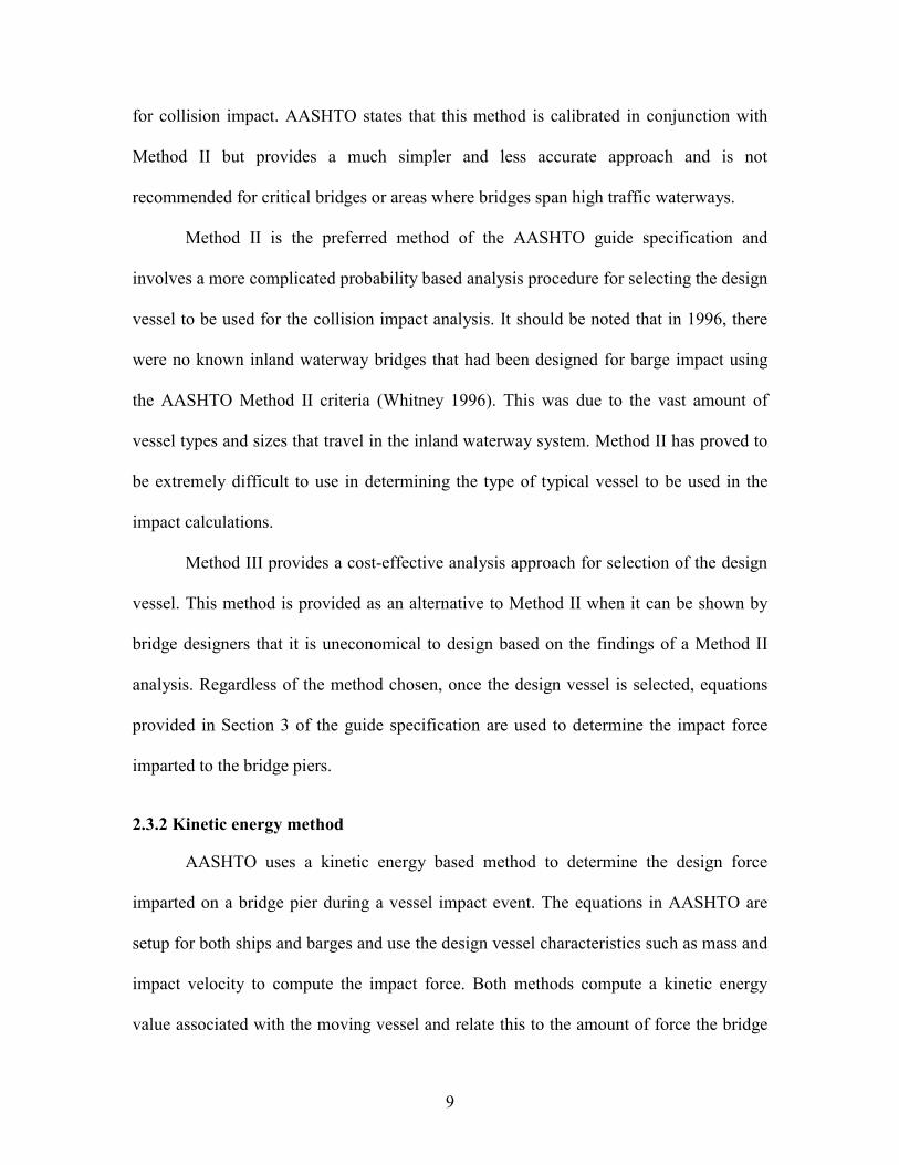
Figure 2-1 Impact force versus time relationship used in AASHTO specifications (AASHTO 1991)
Figure 2-1 shows the relationship between actual impact force versus time and the
equivalent static load magnitude,_P . The static approach provides for a much simpler
load determination method over a dynamic analysis of the impact event. Complete
calculations of the AASHTO kinetic energy method load analysis for the proposed
impact piers of the existing Saint George Island Causeway are presented in Appendix A.
11
2.3.3 Experimental basis for AASHTO barge impact force equations
The equations for computing the impact force for ship and barge impact loads are
derived from various experiments conducted mostly in the late 1970’s and early 1980’s.
There have been several experiments conducted in the area of ship-to-ship and ship-to-
rigid body collisions. Most of the studies on ship-to-ship collision were performed as
scale model experiments. Results from these tests were studied to understand the
mechanics of energy loss during impact as well as to characterize the deformations and
impact forces with respect to time. However, little data is available on the mechanics of
collisions involving barge tows (AASHTO 1991). The equations provided for
determining barge impact loads were derived from one set of experiments that were
conducted in Germany in 1983 (AASHTO 1991). These experiments consisted of
pendulum hammer tests on scaled-down barge segments, typical of standard European
hopper barges. The tests were performed to obtain a better understanding of the
relationship of barge deformation and energy dissipation.
None of the experiments relating to either ships or barges involved the simulation
of impacts on bridge support structures or other non-rigid structures. In the case of
impacts with rigid bodies (i.e. massive concrete structural walls), all of the energy of the
collision is consumed as plastic deformation occurs in the impacting vessel. However, in
the more complex case of a vessel colliding with a deformable (i.e. non-rigid) bridge pier,
the impact does not behave like the simpler rigid body case. Energy dissipation will arise
due to deformation of the impacting vessel, but also due to crushing of the bridge pier
and displacement of the soil surrounding the bridge piles. The less ideal, more realistic
impact case yields lower impact forces, longer impact durations, and less vessel
deformations than the ideal rigid case (Larsen 1993). The impact force equations given in
12
the AASHTO guide specification predict a resultant force based on empirical formulas
for determining the crushing depth of the vessel bow. Since the equations are derived
from experiments corresponding to the ideal rigid impact case, they predict forces that are
likely much higher than those actually produced in true vessel collisions.
In recent years, bridge designs in the state of Florida have largely been governed
by the requirements of the AASHTO design specification and commentary for vessel
impact. Due to this fact and due to the uncertainty in the basis of the design
specifications, the Florida Department of Transportation (FDOT) is sponsoring a research
project in which full-scale impact tests of a jumbo hopper barge will potentially be
performed on the Saint George Island Causeway Bridge. The goal of this research is to
carefully quantify and characterize the loads imparted by barges to bridges during impact
events.
2.4 Previous experimental impact tests
As stated above, there have only been a limited number of tests performed that
served to quantify the impact characteristics of a collision between a barge and bridge
pier. A review of previous experimental tests is presented below.
The most recent set of testing conducted with regard to barge impact loads was
performed by the Army Corps of Engineers Waterways Experiment Station in 1999.
These tests involved full-scale impact testing of barge tows colliding with outer lock
walls in inland waterways. The tests utilized a fifteen-barge tow impacting the lock wall
structures at low velocities and oblique angles. The intent of the testing program was to
determine the impact loading history imparted to the lock wall and the interaction
between the individual barges in the tow during the impact. At the time of this
13
publication, the final results of the Army Corps of Engineers testing have not been
published. Also, due to the nature of these impact tests, they are not appropriate for
correlation with head on impacts with bridge piers.
Probably the most notable research that has been conducted in the way of
determining impact load characteristics associated with barges was performed in 1983 in
West Germany (Meir-Dornberg 1983). The research was conducted to gain a better
understanding of the force and deformation of barges when they impact lock walls and
bridge piers. The study included dynamic loading experiments with a pendulum hammer
on three scale models of barge bottoms and one static loading experiment on another
scale model of a barge bottom. The tests revealed no significant differences between the
dynamic and static forces that were measured in the study. The results from the
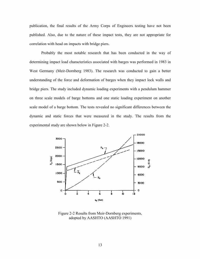
experimental study are shown below in Figure 2-2.
Figure 2-2 Results from Meir-Dornberg experiments, adopted by AASHTO (AASHTO 1991)
14
This chart can also be found in the AASHTO Guide Specification and
Commentary for Vessel Collision Design of Highway Bridges. Figure 2-2 above relates
the barge material crush depth, aB to impact force, PB. The top curve, PB is the result of
the dynamic impact hammer tests and the lower line, BP is the result of the static load
test. These results from Meir-Dornberg’s experiments were used by AASHTO to develop
equations for computing impact forces associated with barge collision events.
In addition to full-scale testing, some research has been done in the way of
numerical modeling and approximation of barge impact events. The most recent study
was conducted by researchers at Florida State University in Tallahassee, Florida in 1999
(Weckezer 2000). This research involved the numerical modeling of a jumbo hopper
barge and timber fender whales used for bridge pier protection. The intent of the research
was to develop a better design for fender systems to resist low velocity, oblique impacts
from barge tows. Another example of numerical research work can be found in the Army
Corps of Engineers, Engineering Technical Letter 1110-2-338 (ETL 338). The paper
presents a numerical model for approximating the impact force imparted by barge tows
on rigid and flexible structures (Patev 1999). ETL 338 treats the barge tow and impacted
structure as a single degree of freedom (SDOF) system for purposes of analysis. An
actual barge tow, which usually made up of several barges and a tug, has multiple
degrees of freedom. This approximation of a multiple degree of freedom (MDOF)
problem with a SDOF analysis is the basis and motivations of the research that is being
performed by Robert Patev and the Army Corps of Engineers discussed earlier. The full
scale testing will help to validate the accuracy of the SDOF system model presented in
ETL 338.
15
Finally, the basis for all current research, experimental or numerical, is the testing
performed by Minorsky (Minorsky 1959). V.U. Minorsky conducted full-scale impact
tests on ship hulls for purposes of protecting nuclear powered ships against ship-to-ship
and ship-to-structure impact incidents. Minorsky determined a relationship between the
kinetic energy absorbed during an impact event to the volume of damaged steel that
resulted from the impact (Patev 1999). This relationship is used by most all research
conducted in the area of vessel collision analysis, including the AASHTO guide
specification.
16
CHAPTER 3 PROPOSED TEST PROGRAM AND IDENTIFICATION OF
FEASIBILITY ISSUES
3.1 Overview of proposed experimental testing
The literature search described in the previous chapter did not reveal any
published reports of full scale experimental tests involving barges impacting bridge piers.
Since bridges spanning navigable waterways must be designed to resist barge impact
loading, directly quantifying the loads associated barge impacts—through the use
experimental testing—is highly desirable. As was briefly described in Chapter 1, the
replacement of the existing St. George Island causeway bridge affords a unique
opportunity to conduct experimental barge impact testing on a full scale structure after it
has been taken out of service.
The existing St. George Island causeway bridge spans from Rt. 98 (near
Eastpoint, Florida) to St. George Island in Apalachicola, Florida. Near the middle of the
overall bridge length lies a small island that effectively splits the bridge into separate
northern and southern sections (see Figure 3-1).
The navigation channel for the Intracoastal Waterway (ICWW) runs beneath the
southern section of the bridge and therefore it is this section that will be used to conduct
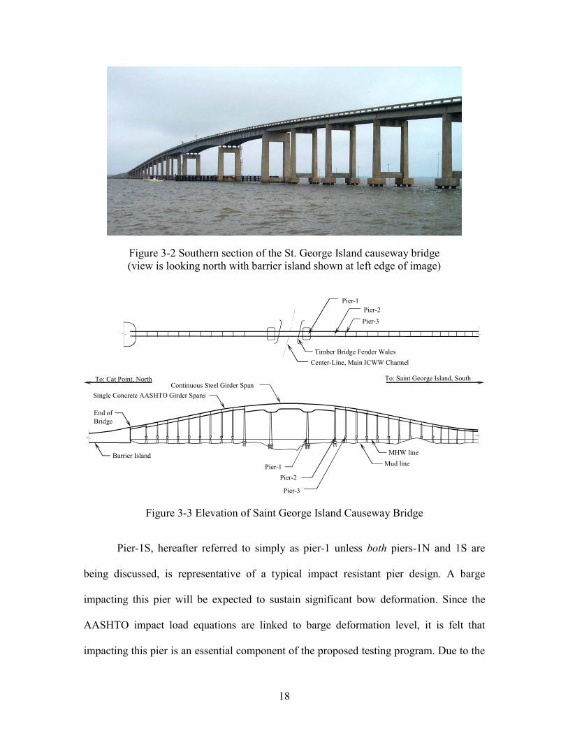
the proposed barge impact testing (see Figure 3-2). A three-span continuous steel girder
bridge segment in the southern section spans over both the navigation channel and the
areas directly adjacent to the channel (see Figure 3-3). Simple-span pre-stressed girder
segments make up the remainder of the southern portion of the bridge.
17
NO
RTH
Intracoastal Waterwaychannel
Cat point
St. George Island
Barrier Island
North Bridge
South Bridge
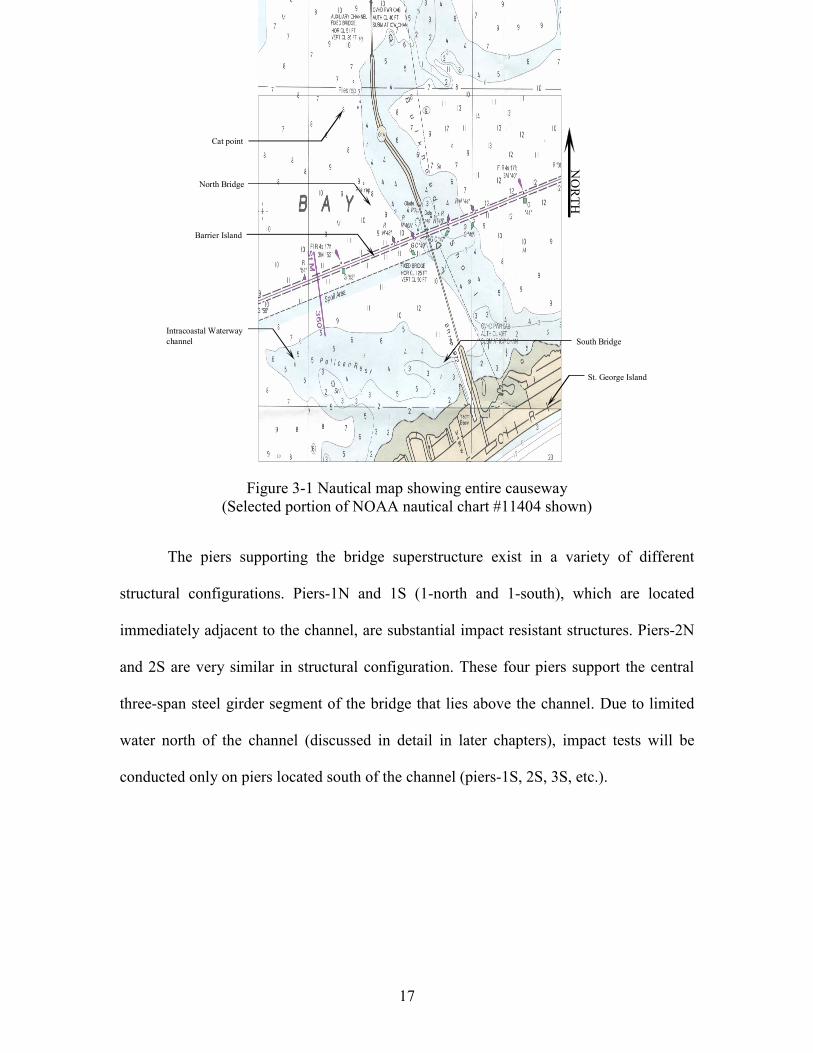
Figure 3-1 Nautical map showing entire causeway (Selected portion of NOAA nautical chart #11404 shown)
The piers supporting the bridge superstructure exist in a variety of different
structural configurations. Piers-1N and 1S (1-north and 1-south), which are located
immediately adjacent to the channel, are substantial impact resistant structures. Piers-2N
and 2S are very similar in structural configuration. These four piers support the central
three-span steel girder segment of the bridge that lies above the channel. Due to limited
water north of the channel (discussed in detail in later chapters), impact tests will be
conducted only on piers located south of the channel (piers-1S, 2S, 3S, etc.).
18
Figure 3-2 Southern section of the St. George Island causeway bridge (view is looking north with barrier island shown at left edge of image)
To: Saint George Island, SouthTo: Cat Point, North
Center-Line, Main ICWW ChannelTimber Bridge Fender Wales
Continuous Steel Girder SpanSingle Concrete AASHTO Girder Spans
MHW line
End ofBridge
Barrier IslandMud line
Pier-3
Pier-1
Pier-1
Pier-3
Pier-2
Pier-2
Figure 3-3 Elevation of Saint George Island Causeway Bridge
Pier-1S, hereafter referred to simply as pier-1 unless both piers-1N and 1S are
being discussed, is representative of a typical impact resistant pier design. A barge
impacting this pier will be expected to sustain significant bow deformation. Since the
AASHTO impact load equations are linked to barge deformation level, it is felt that
impacting this pier is an essential component of the proposed testing program. Due to the

19
structural rigidity and strength of this pier, it will also be able to sustain barge impacts at
higher velocities than will other lesser piers in the bridge. Thus, the largest magnitude
impact forces to be measured will occur during tests conducted on this pier.
In contrast to piers-1 and 2, both of which are structurally very substantial, pier-3
is a more flexible and weaker structure. Pier-3 represents a typical “secondary pier” that
is not designed to be impact resistant (at impact velocities typical of channel traffic). As
opposed to pier-1 which uses a single massive pile cap to tie the piles to the pier columns,
pier-3 uses two much smaller isolated caps instead. It is proposed that barge impacts be
conducted on pier-3 but at velocities well below those used to test pier-1. As will be
discussed in greater detail later in the report, the impact velocities chosen for pier-3 will
be selected so as not to fail the pier during the impacts. However, the pier is expected to
deform much more than pier-1 and little deformation of the barge bow is expected to
occur during these tests. Thus, by testing both pier-1 and pier-3, an adequate range of
barge and pier deformation levels will be covered by the impact tests conducted.
3.1.1 Instrumentation for measurement of impact loads
During the Phase I feasibility study, a meeting was held with representatives from
the U.S. Army Corps of Engineers regarding barge impact tests that had previously been
conducted on lock walls (Patev 1999). The intent of the meeting was to determine
whether the instrumentation methods used in these earlier tests would be applicable to
situations involving barge-to-pier impact.
Several differences exist between the Army Corps tests and the test proposed for
the St. George Island causeway bridge. The Army Corps tests consisted of glancing
impacts in which the nearly rigid corner of the barge bow impacted the lock wall. After

20
impact, the barge was redirected away from the wall (i.e. “glanced” off the wall) with
very little reduction in velocity and nearly zero deformation of the barge bow. In contrast,
the tests proposed for the St. George Island causeway bridge will consist of head-on
impacts in which the barge will contact the bridge pier at a point very near to the center
of the barge headlog (i.e. at the middle of the barge bow). Significant deformation of the
barge bow is expected in some of the impact tests that will be conducted. In addition,
rather than consisting of glancing blows with little reduction in barge velocity, the head-
on impacts to be conducted on the St. George Island causeway bridge piers will bring the
barge to a complete stop after impact and will produce impact forces much larger than
those measured during the Army Corps tests.
As a result of the meeting with the Army Corps representatives, it was concluded
that the device they used to measure impact loads is not applicable to the case of barge-
to-bridge impact. However, several design concepts for alternative methods of load
measurement were generated during the meeting and appear to have promise. One of the
systems presently being considered is shown in Figure 3-4. The device consists of a
collection of load cells mounted between two structural steel pressure plates. One
pressure plate allows the device to mounted at the desired position on the bridge pier
while the other pressure plate (nearer the impact face) allows a sacrificial concrete block
to be attached. The system will be bolted to the piers at the desired elevation. A key
feature of this concept is that it permits direct measurement of impact forces without
altering the stiffness of the barge headlog. Also, the sacrificial concrete block mimics the
structural stiffness of the pier column and can be replaced if it is severely damaged
during an impact test.

21
Much greater focus and effort will be placed on the design and development of
instrumentation systems in Phase II of this project. However, at the conclusion of the
Phase I feasibility study, the authors are confident that it is feasible to develop a system
capable of measuring the loads that will be generated during the proposed test program.
Impacting Jumbo Hopper Existing bridge pier to be used for impact
Anchor bolts grouted into pier for easy replacement of instrumentation pack
Water Line
Sacrificial concrete
Load cells
Figure 3-4 Conceptual design of a device capable of measuring impact loads between a barge bow and a bridge pier
3.1.2 Proposed schedule for full-scale impact experiments
In order to maximize the usefulness of the impact force data collected, it is
proposed that the full scale test program for the St. George Island causeway bridge be
conducted in three stages. These stages will permit the measurement of loads on impact
resistant piers, on non impact resistant piers, on piers connected to adjacent piers through
the bridge super structure, and on isolated piers.
In the first stage of impact testing, a portion of the bridge superstructure will be
left in place linking pier-3 to both pier-2 and pier-4 (see Figure 3-5). Impact tests will be
conducted at low velocities such that only minimal damage is done to the barge bow and
pier-3. The superstructure segments left in place will be isolated such that only
22
neighboring piers will remain connected to pier-3. Also, as a safety precaution, the main
span continuous steel girders will be removed prior to the first stage of testing so that
there is no chance of debris falling into the navigation channel as a result of the impact
testing.
At Least One ConcreteGirder Span Removed
Continuous Steel Girder Span Removed
Pier-3
Pier-2 Pier-4
Figure 3-5 Bridge configuration during stage-1 impact tests
The second stage of impact testing will be conducted on the impact resistant
pier-1. This series of tests will be conducted just following the conclusion of the stage
one impact experiments. Channel pier-1 will be subjected to barge impacts as an isolated
structure (see Figure 3-6) and will be conducted at higher velocities than the stage one
tests. Significant deformation of the barge bow and large impact forces are expected to
occur during this stage of testing.
At Least One ConcreteGirder Span Removed
Continuous Steel Girder Span Removed
Pier-1
Figure 3-6 Bridge configuration during stage-2 impact tests
23
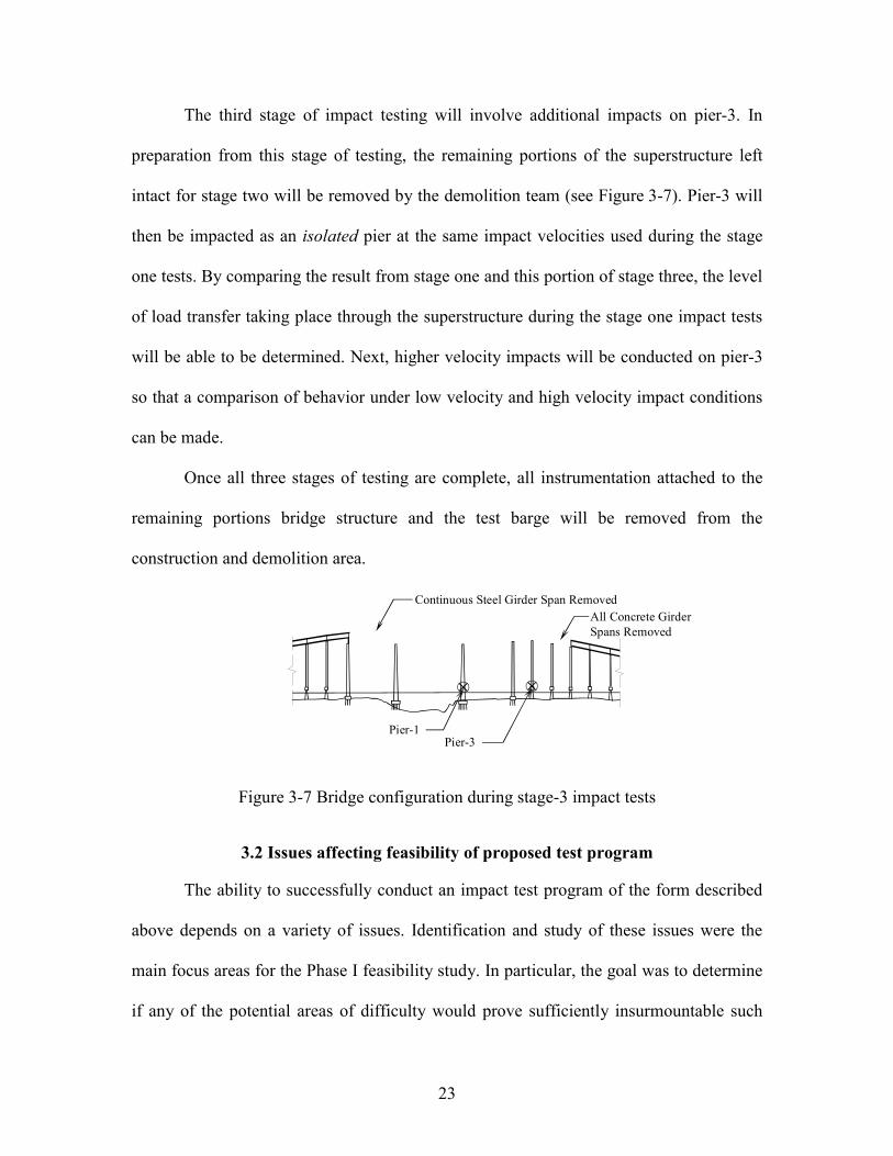
The third stage of impact testing will involve additional impacts on pier-3. In
preparation from this stage of testing, the remaining portions of the superstructure left
intact for stage two will be removed by the demolition team (see Figure 3-7). Pier-3 will
then be impacted as an isolated pier at the same impact velocities used during the stage
one tests. By comparing the result from stage one and this portion of stage three, the level
of load transfer taking place through the superstructure during the stage one impact tests
will be able to be determined. Next, higher velocity impacts will be conducted on pier-3
so that a comparison of behavior under low velocity and high velocity impact conditions
can be made.
Once all three stages of testing are complete, all instrumentation attached to the
remaining portions bridge structure and the test barge will be removed from the
construction and demolition area.
All Concrete Girder Spans Removed
Continuous Steel Girder Span Removed
Pier-1Pier-3
Figure 3-7 Bridge configuration during stage-3 impact tests
3.2 Issues affecting feasibility of proposed test program
The ability to successfully conduct an impact test program of the form described
above depends on a variety of issues. Identification and study of these issues were the
main focus areas for the Phase I feasibility study. In particular, the goal was to determine
if any of the potential areas of difficulty would prove sufficiently insurmountable such

24
that the test program cannot be completed at the St. George Island site. In order to
generate the list of feasibility issues to investigate, discussions were held with several
FDOT engineers, FHWA, the St. George Island design/build entity Sverdrup/Boh
Brothers, the U.S. Army Corps of Engineers, and others. Based on these discussions, the
following list of feasibility issues was generated for further study.
• Environmental permits for the proposed testing
• Acquisition and modification of a hopper barge of appropriate size and type
• Choice of barge navigation paths that provide sufficient water depth to avoid
grounding and also avoid obstacles such as power lines
• Integration of barge testing activities into the contractor’s demolition schedule
• Establishment of preliminary impact test conditions including selection of piers to
be impacted, mass of barge cargo, and impact velocities
Each of these areas is discussed in greater detail in the chapters that follow.
25
CHAPTER 4 ENVIRONMENTAL PERMITTING
4.1 Introduction
There are many environmental concerns associated with impact testing and
demolition of the existing Saint George Island Causeway Bridge. The causeway is
located in the middle of Apalachicola Bay, which has been identified as an Outstanding
Florida Water, an Aquatic Preserve, a Surface Water Improvement and Management
priority water body, and the largest National Estuarine Research Reserve in the United
States. Most of the bay, including the areas surrounding the existing bridge, is designated
as Class II Shellfish Propagation and/or Harvesting Water. Thus, there are high water
quality standards in place for the bay. Productive oyster beds, shallow water, and local
wild life in the area of the existing bridge present added concerns for the impact-testing
program.
Due to the conditions present in Apalachicola Bay, it is essential that any testing
activities be conducted with a high level of environmental awareness. In the sections that
follow, details of the relevant environmental issues relating to the feasibility of the
proposed barge impact testing program are presented.
4.2 Oyster Beds
The Apalachicola Bay produces a large percentage of the oysters harvested in
Florida. The oyster bars cover approximately 10,600 acres of bay bottom within the
Apalachicola Natural Estuarine Research Reserve. Furthermore, the existing bridge
alignment is over the most productive natural oyster bar found in the bay. In an effort to
reduce the impact to the oyster crop, oyster relays have already been coordinated and

26
carried out by professional oystermen. The oyster relays were conducted in the months
of July, August, and September of 2000 when the area is normally open for harvesting.
The purpose of the relays was to relocate vital oyster beds away from the construction
and demolition areas and preserve their safety. There is also a possibility that a final
relay will take place just prior to the demolition of the existing bridge.
The major concern in harming the oyster beds is adverse turbidity in the waters
where the beds are located. If the oyster beds become buried by sediment, they can
potentially die. The largest causes of turbidity from vessel movements are grounding of
the vessels and propeller wash created when traveling at high velocities. In an effort to
reduce potentially damaging effects to the thriving oyster beds of Apalachicola bay, a
series of precautions and restrictions will be implemented for the barge impact testing
program. Most of the vessel movements associated with the testing will take place inside
or near the Intracoastal Waterway (ICWW) channel. Where barge traffic routinely passes
on a daily basis. Vessel movements in or near the ICWW channel will not create any
increased effect on the oysters. In addition, a shallow draft tug that has a protective
shroud installed around its propeller will be used to propel and guide the test barge. The
shallow draft of the tug will ensure that grounding does not occur while the protective
shroud around the propeller will ensure no chopping of the bay bottom by the propeller
occurs and also serves to reduce adverse turbidity effects. The test barge will also be at a
shallow draft condition to eliminate the chances for vessel grounding. A comprehensive
bathymetric survey was conducted by the authors to verify that the water depth around
the existing bridge is sufficient to permit the testing without danger of grounding the test
barge. Details of this survey are given in Chapter 6.

27
4.3 Manatees and Protected Bird Estuaries
Apalachicola Bay is home to some of Florida’s endangered species, the Gulf
Sturgeon and the West Indian Manatee. These endangered species are present in the bay
from the months of November through April each year. In order to protect these
endangered species, the impact testing experiments will be conducted during the months
of May through August and will not affect the endangered species.
In addition to the endangered species in the water, the island between Cat Point
and Saint George Island is home to protected bird wildlife. The demolition of the bridge
will include the creation of an estuary on the island between Cat Point and Saint George
Island. The current permit documentation for the construction of the new replacement
bridge and demolition of the existing bridge set restrictions on construction activities for
the island for the bird nesting season in the Apalachicola Bay Estuarine. The impact
testing program will have no activities that involve the island between the north and south
bridges. Therefore, the barge impact testing program is expected to have no affect to the
protected bird wildlife in the Apalachicola Bay Esturarine.
4.4 Noise Levels Associated with Impact Testing
Physical impact testing of the bridge structure will produce noticeable, but short
duration airborne and waterborne noise. The noise created during the impact events is an
issue mainly due to potential harm to aquatic life around the bridge. To reduce the
chances of harming wildlife, no impact tests will be conducted during the months from
November to April due to the potential presence of the Gulf Sturgeon or the West Indian
Manatee. The importance of these species was discussed above. Also, since the noise
28
associated with the impact testing is very short in duration and with a very small number
of incidents, no adverse affects on wildlife is expected.
Permits have been obtained by the bridge demolition team that authorizes the use
of controlled explosives during the removal of the main channel piers. The fact that the
demolition team was able to obtain this permit, and in such a sensitive region, servers as
evidence that a permit for the much less noisy barge impact testing will be easily
acquired.
4.5 Falling Debris Containment
The current construction and demolition permit documents strictly state that
dumping of construction waste material into the bay or debris from construction and/or
demolition activities falling into the bay are prohibited. The reasons for this restriction
include the possibilities of introducing pollutants into the water and the potential for
burying oyster beds under falling debris. As discussed in Section 4.1, the oyster beds can
be harmed and in some cases even killed if buried. In light of these permit restrictions,
the impact testing program will be conducted in such a fashion to minimize the amount of
debris that fall into the bay. Large tarps will be installed under the testing pier(s) during
the testing events to catch any concrete that is spalled off due to the impacting barge. In
addition to this, Phase II of the impact testing program involves the development of an
instrumentation scheme for the barge and bridge. The proposed instrumentation package
for the test piers will include a section of concrete attached to the measurement devices.
This concrete will be designed as a sacrificial element, so that any damage that results
from the impact will be to this sacrificial concrete and not to the pier, thus minimizing the
potential for falling debris.
29
4.6 Proposed Permit Acquisition Process
Acquisition of the necessary permits required for the barge impact testing
program is scheduled to begin at the start of Phase II of the impact testing program,
which starts in January 2002. It is expected that the permit acquisition process will not
require any longer than one year to complete. However, by starting the process as early
as January 2002, it is possible for the permitting process to take up to as long as one and a
half years and not affect the impact testing schedule.
Permits for the barge impact testing program will need to be obtained by the
following government agencies, The Coast Guard, The Army Corps of Engineers, and
The Florida Department of Environmental Protection. In addition, there may also be
some local agency permits that will need to be obtained as well for the testing program.
Due to the research team’s lack of knowledge in the area of permit acquisition, it is being
proposed that an outside engineering consulting firm be contracted to obtain all the
necessary permits required for the barge impact testing program. In discussions with the
engineer of record for the replacement bridge, Jacob Sverdrup, Inc., has agreed to present
the research team and the FDOT with a proposal for conducting the permit acquisition
process of the testing program. Jacob Sverdrup, Inc. would be a good firm to handle the
permit acquisition process since they just recently went through the process to obtain the
permits for the replacement bridge.
30
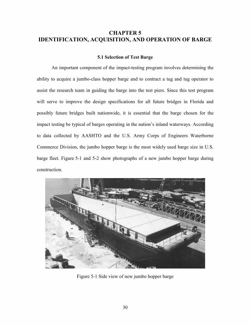
CHAPTER 5 IDENTIFICATION, ACQUISITION, AND OPERATION OF BARGE
5.1 Selection of Test Barge
An important component of the impact-testing program involves determining the
ability to acquire a jumbo-class hopper barge and to contract a tug and tug operator to
assist the research team in guiding the barge into the test piers. Since this test program
will serve to improve the design specifications for all future bridges in Florida and
possibly future bridges built nationwide, it is essential that the barge chosen for the
impact testing be typical of barges operating in the nation’s inland waterways. According
to data collected by AASHTO and the U.S. Army Corps of Engineers Waterborne
Commerce Division, the jumbo hopper barge is the most widely used barge size in U.S.
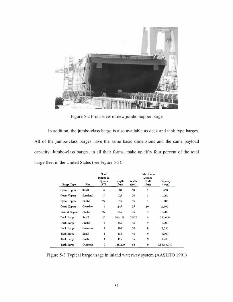
barge fleet. Figure 5-1 and 5-2 show photographs of a new jumbo hopper barge during
construction.
Figure 5-1 Side view of new jumbo hopper barge
31
Figure 5-2 Front view of new jumbo hopper barge
In addition, the jumbo-class barge is also available as deck and tank type barges.
All of the jumbo-class barges have the same basic dimensions and the same payload
capacity. Jumbo-class barges, in all their forms, make up fifty four percent of the total
barge fleet in the United States (see Figure 5-3).
Figure 5-3 Typical barge usage in inland waterway system (AASHTO 1991)
32
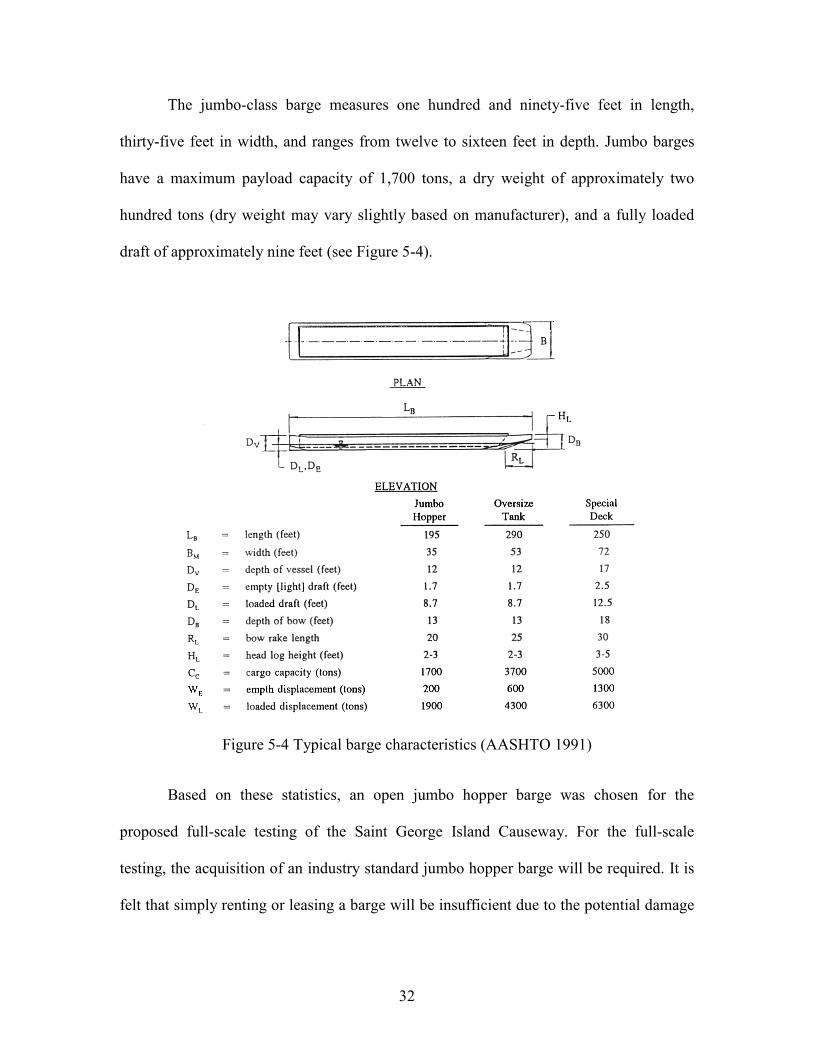
The jumbo-class barge measures one hundred and ninety-five feet in length,
thirty-five feet in width, and ranges from twelve to sixteen feet in depth. Jumbo barges
have a maximum payload capacity of 1,700 tons, a dry weight of approximately two
hundred tons (dry weight may vary slightly based on manufacturer), and a fully loaded
draft of approximately nine feet (see Figure 5-4).
Figure 5-4 Typical barge characteristics (AASHTO 1991)
Based on these statistics, an open jumbo hopper barge was chosen for the
proposed full-scale testing of the Saint George Island Causeway. For the full-scale
testing, the acquisition of an industry standard jumbo hopper barge will be required. It is
felt that simply renting or leasing a barge will be insufficient due to the potential damage
33
that may occur to the bow of the barge from the impact testing. Thus, the Department will
need to purchase a new or used jumbo-class open hopper barge.
5.1.1 Special considerations for use of aging barges
In the event that the Department chooses to purchase a used or aging barge, there
are some special concerns that will need to be addressed in reference to the condition of
the barge. There are two areas of concern in selecting an aging barge with respect to the
impact testing. First, an assessment must be made of the weakened bow strength if the
barge is in a rusted, deteriorated condition. Second, in order for the barge to be useful, its
head log must be undamaged. There are also problems associated with an aging barge
with respect to the overall safety of the testing program. Steel in an aging barge will
likely be rusted and more brittle than that of a new barge. This could lead to reduced
stiffness and also failure of structural components in the barge bow. If severe enough,
such damage could lead to a condition in which the barge would no longer float after
impact. For safety reasons, this must be avoided. Careful examination of the candidate
barge must occur in order to assess its condition before a purchase is made.
5.2 Estimated Barge Acquisition Costs
A price quote for the construction of a new jumbo-class open hopper barge was
obtained from one of the nation’s leading barge manufacturers, Trinity Marine, Inc.
Trinity has five barge manufacturing facilities within the United States and the ability, at
full capacity, to produce jumbo-class hopper barges at a rate of one per day. The price
quote for a typical hopper with no modifications or cargo covers was $245,000 dollars.
The estimated production time was six to nine months from time of order depending on
material availability.
34
The costs of used open hopper barges range from $120,000 dollars to $60,000
dollars. These costs are based upon discussions with the sales staff at Trinity Marine, Inc.
and based on Internet searches for used barges for sale during the year 2001. Aging
barges decrease in overall structural integrity proportionally with cost. A jumbo-class
open hopper barge in good condition should be obtainable for approximately $100,000
dollars. Any used barges considered for use in the impact testing must be carefully
examined based on the conditions discussed in the previous section. The estimated time
to acquire a used barge is highly variable, ranging from a few months to over a year.
Acquisition time is dependent on the market availability of used barges that are in
acceptable condition.
It should be noted that after impact testing is complete, the test barge will likely
be sold. Income generated by this sale will serve to offset the costs associated with its
initial purchase. If the barge is still in operational condition, it could possibly be sold
intact. However, in the event the barge is damaged beyond repair, it can still be sold as
scrap metal.
5.3 Tug Requirements for Conducting the Test Program
In addition to the acquisition of a barge, a tug and tug operator will be needed to
maneuver and guide the barge throughout the duration of the testing program. Based on
the environmental concerns discussed in Chapter 4, the tug will need to be a shallow draft
tug and have a protective metal shroud around its propeller housing. In preliminary
discussions with the contractor, Boh Brothers Construction Co., the possibly using one of
their shallow draft tugs and operators is being considered. Figure 5-5 shows a shallow
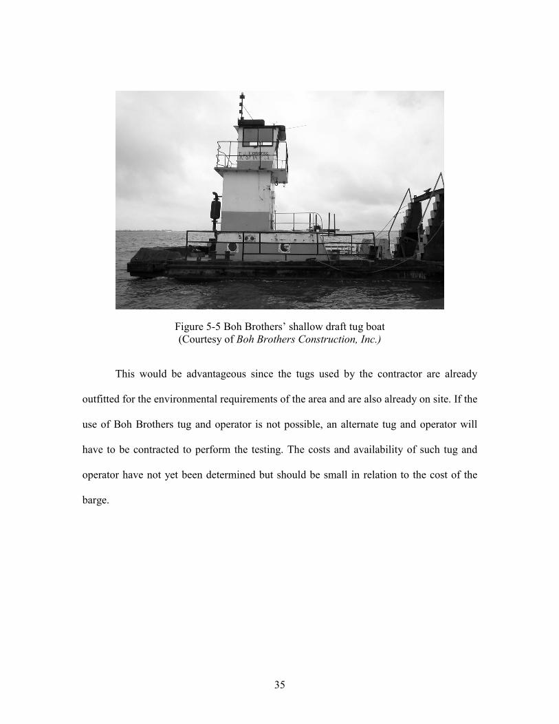
draft tug boat in use at the Boh Brothers construction site in Apalachicola Bay.
35
Figure 5-5 Boh Brothers’ shallow draft tug boat (Courtesy of Boh Brothers Construction, Inc.)
This would be advantageous since the tugs used by the contractor are already
outfitted for the environmental requirements of the area and are also already on site. If the
use of Boh Brothers tug and operator is not possible, an alternate tug and operator will
have to be contracted to perform the testing. The costs and availability of such tug and
operator have not yet been determined but should be small in relation to the cost of the
barge.
36
CHAPTER 6 GEOGRAPHICAL ISSUES
6.1 Introduction
In addition to the issues associated with environmental permitting and acquisition
of a test barge and operator, there were some aspects of the proposed test bridge’s
physical location that needed to be addressed. The first concern was whether or not the
water depths in the bay area surrounding the bridge would inhibit the ability to conduct
the testing experiments. Due to the environmental sensitivity of the Apalachicola bay
area, it was critical to determine the water depth around the test piers and along the
testing barge approach path to ensure that no grounding of the barge will occur.
To prevent grounding, it was desired to acquire accurate water depth data for the
bay bottom in the areas where the proposed testing will take place. However, attempts to
locate data pertaining to recent depth surveys of the bay bottom in the areas around the
existing bridge alignment failed. In order to achieve confidence in the bay depth data
used, the research team from the University of Florida and a representative from the
FDOT conducted a bathymetric survey of the area. A description of the bathymetric
survey and the results are discussed in more detail in Section 6.2. The second
geographical concern for the testing program pertained to the proposed bridge
alignment’s location with respect to the existing bridge alignment. The distance between
the proposed and existing bridge alignments was critical to determining whether or not it
would be possible to conduct the testing without having to navigate the test barge
between piers of the new bridge alignment.

37
6.2 Bathymetric Survey Results
In order to obtain accurate water depth data for the area under and around the
existing bridge alignment, the University of Florida conducted a bathymetric survey of
the bay bottom. The survey was conducted using conventional global positioning satellite
(GPS) and sonar based depth measurement equipment. Special attention was given to the
waters between the existing and proposed bridge alignments. The GPS and depth data
were then plotted using a contour smoothing routine. The results are presented below in
Figure 6-1.
Existing BridgeAlignment
New BridgeAlignment
Figure 6-1 Bathymetric Survey conducted by University of Florida (Contour elevations in ft.)
Based on the results of the bathymetric survey, we are confident that a jumbo
hopper barge loaded at half capacity, drafting four to five feet would have no trouble
navigating the waters between the new and existing bridge alignments and around the
38
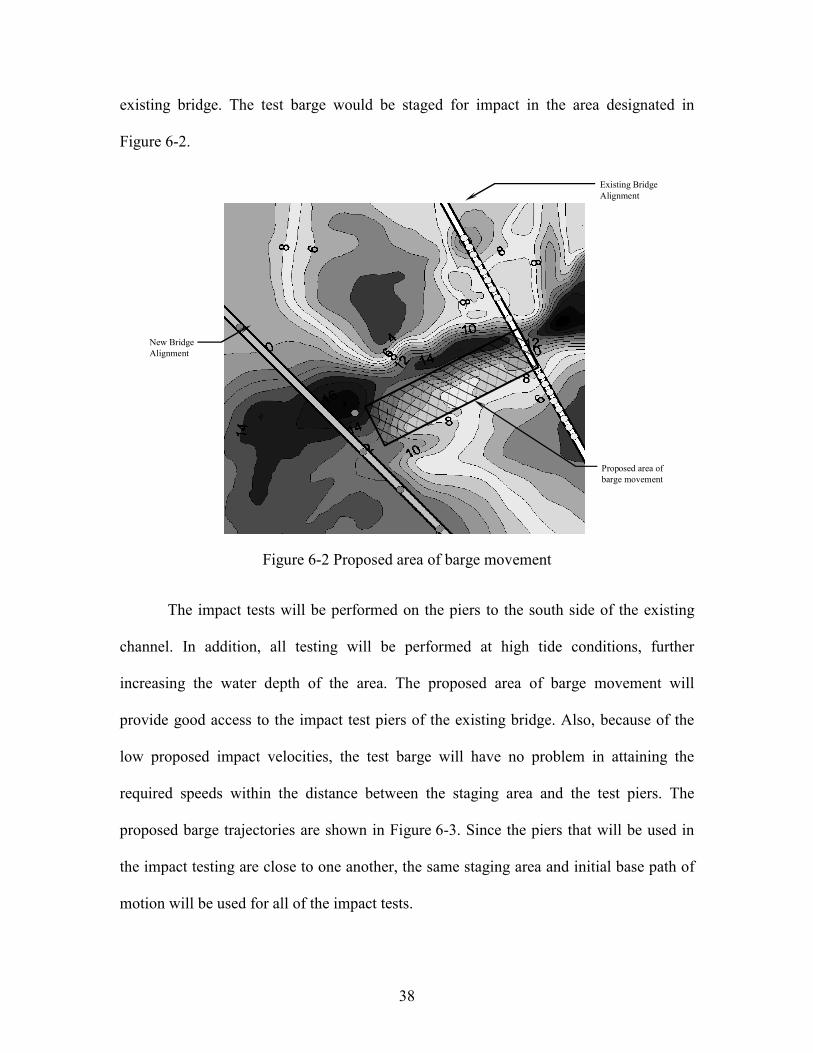
existing bridge. The test barge would be staged for impact in the area designated in
Figure 6-2.
Existing BridgeAlignment
New BridgeAlignment
Proposed area ofbarge movement
Figure 6-2 Proposed area of barge movement
The impact tests will be performed on the piers to the south side of the existing
channel. In addition, all testing will be performed at high tide conditions, further
increasing the water depth of the area. The proposed area of barge movement will
provide good access to the impact test piers of the existing bridge. Also, because of the
low proposed impact velocities, the test barge will have no problem in attaining the
required speeds within the distance between the staging area and the test piers. The
proposed barge trajectories are shown in Figure 6-3. Since the piers that will be used in
the impact testing are close to one another, the same staging area and initial base path of
motion will be used for all of the impact tests.

39
Existing BridgeAlignment
New BridgeAlignment
Proposed area ofbarge movement
Primary pier impacttesting trajectory
Secondary pier impacttesting trajectory
Figure 6-3 Proposed trajectories for impact tests
The results from the bathymetric survey indicate that the full-scale impact testing
of the Saint George Island Causeway Bridge is feasible from a geographical standpoint of
the current water depth conditions. In discussions with the contractor, it was learned that
the bay bottom around the testing area is changing. In the event that the area was to be hit
by a hurricane, the water conditions would be greatly affected also. Thus, it will be
necessary to conduct another bathymetric survey of the area of barge movement just prior
to the full-scale impact testing in the summer of 2003.

40
CHAPTER 7 SCHEDULING
7.1 General Scheduling Requirements
The completion of the environmental permitting process and the integration of the
testing program into the demolition schedule of the existing causeway must be
accomplished in order for the testing programs to be a success. Full-scale testing will
need to be conducted during the summer months of 2003 in order to coincide with the
current demolition schedule for the causeway. Environmentally, the testing program is
limited to the months of April to November (discussed in detail in Chapter 4). Thus, the
physical impact experiments will be conducted in the months of April to July of 2003. In
addition, there are many more tasks that require completion before physical testing can
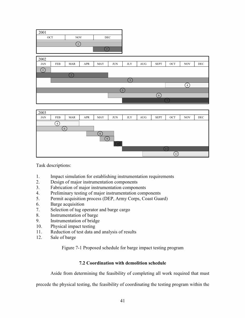
occur. Figure 7-1 shows a proposed schedule of tasks associated with the barge impact
testing program. The proposed schedule spans from October 2001 to December 2003 and
outlines the estimated times need to complete each required task.
At this stage in the testing program, it is feasible to complete all the required tasks
in preparation for the full-scale impact experiments in the time available. For example,
the permitting process, which traditionally requires a considerable amount of time to
complete, has been allocated one year for completion. However, based on the current
schedule, this process could potentially run as long as four to five months beyond the
allotted year and still not interfere with the overall schedule and success of the testing
program.
41
JAN FEB MAR APR MAY JUN JLY AUG SEPT OCT NOV DEC
1
2
3
4
5
6
7
2002
2001OCT NOV DEC
1
2
JAN FEB MAR APR MAY JUN JLY AUG SEPT OCT NOV DEC2003
4
6
8
9
10
11
12
Task descriptions: 1. Impact simulation for establishing instrumentation requirements 2. Design of major instrumentation components 3. Fabrication of major instrumentation components 4. Preliminary testing of major instrumentation components 5. Permit acquisition process (DEP, Army Corps, Coast Guard) 6. Barge acquisition 7. Selection of tug operator and barge cargo 8. Instrumentation of barge 9. Instrumentation of bridge 10. Physical impact testing 11. Reduction of test data and analysis of results 12. Sale of barge
Figure 7-1 Proposed schedule for barge impact testing program
7.2 Coordination with demolition schedule
Aside from determining the feasibility of completing all work required that must
precede the physical testing, the feasibility of coordinating the testing program within the
42
demolition schedule of the existing causeway needed to be assessed as well. A meeting
was held at the construction site for the replacement bridge on October 4th, 2001. In
attendance were, the University of Florida research team and representatives from the
Florida Department of Transportation, Boh Brothers Construction, Inc. (construction and
demolition contractor) and Jacob Sverdrup, Inc.(replacement bridge engineers). The
purpose for the meeting was to determine the feasibility of integrating full-scale barge
impact testing of bridge piers in the south bridge of the existing Saint George Island
Causeway Bridge with its demolition schedule. The proposed testing schedule discussed
in Chapter 3 of this report (including the three separate stages of tests), was presented by
the University of Florida research team at the meeting. Based upon responses from the
representatives of Boh Brothers Construction, Inc. and Jacob Sverdrup, Inc., the proposed
schedule for the testing program was feasible with regard to integration into the
demolition schedule.

43
CHAPTER 8 FINITE ELEMENT IMPACT SIMULATION
8.1 Basis for selecting impact conditions
In previous chapters, it has been shown that conducting the proposed impact
testing program is feasible with regard to external factors such as environmental
permitting, barge acquisition, geographic considerations, and scheduling. In the following
chapters, the focus is now shifted to the tasks of determining the optimal set of impact
conditions and ensuring safety during the impact events. In this context, the “optimal
impact conditions” are those conditions that maximize the amount of useful data that can
be collected during testing.
For example, the multiple stages of testing proposed in Chapter 3 involve impacts
on both pier-1 and pier-3 of the bridge. However, pier-3 is not considered to be an impact
resistant pier. In an ideal situation, the cargo mass in the test barge would be changed to
be optimal for each set of pier impacts—more mass for the impact resistant pier-1 and
less mass for pier-3 tests. However, it will not be feasible to alter the barge cargo during
the course of the testing program. Thus, an “optimal” cargo mass condition is sought that
will permit realistically large impact loads to be imparted to pier-1 using moderate impact
velocities but which will also allow for low velocity impacts on pier-1 without
structurally failing this smaller pier.
In addition to choosing the target barge mass, appropriate impact velocities must
be chosen such that the loads imparted to the test piers are in the realm of realistic impact
loads. Since characteristics such as magnitude and time-variation of the impact forces
acting between the barge and pier are a function of barge deformation level, structural
stiffness, and soil stiffness, all of these factors need to be considered in choosing impact
44
mass and velocities. From a safety standpoint, the magnitude of loads imparted to the
piers needs to be estimated so that strength evaluations for these structures can be made.
Also, deformations sustained by the barge bow must not be so severe that they
compromise the buoyancy of the vessel. In order to aid in the acquisition of
environmental permitting and to ensure safety during the tests, the proposed experimental
program will be designed so as to avoid catastrophic failure the piers and sinking of the
barge. Ensuring that such failures do not occur requires that the impact forces associated
with various impact scenarios be quantified.
In order to make decisions and parameter selections of the type just discussed,
computational models must be used to estimate the impact loads that will occur. The
impact load equations contained in the AASHTO provisions provide one such model for
computing impact loads. However, these equations do not provide any information about
the dynamic, time-varying nature of the impact forces generated. What is more, the
AASHTO provisions still require the use of a structural analysis capable of representing
the behavior of the piers, piles, and surrounding soil. The FB-PIER program (Hoit 1996)
permits accurate modeling of pier behavior under lateral loading conditions, but still
requires that the magnitude and time-variation of the lateral loading be specified by the
user.
8.2 Finite element impact simulation
For purposes of predicting not only pier and barge behavior, but also the
magnitude and time-variation of contact forces developed during impact events,
nonlinear impact finite element simulation techniques were used in this research. Only a
small number of finite element codes have all of the capabilities needed to accurately
45
model an impact event as complex as a barge dynamically impacting a bridge pier. Such
a numeric impact simulation must account for dynamic system behavior, detection of
contact between the barge and pier, nonlinear soil-pile interaction, large displacement
nonlinear plastic deformations of barge components, buckling of barge components,
buoyancy effects, gravitational effects, and more.
For this research project, the nonlinear explicit dynamic finite element code
LS-DYNA (LSTC 1999) was chosen as the primary impact simulation tool used. Finite
element models of a jumbo hopper barge, the impact resistant pier-1, and the non-impact
resistant pier-3 were developed for use in establishing appropriate impact parameters for
the proposed test program. Chapters 9 and 10 describe the modeling techniques employed
in the development of these models. Chapter 11 presents results for a variety of different
impact conditions simulated for pier-1 and pier-3 and serves as the basis for the selection
of barge cargo mass and impact velocities to be used in the actual impact testing program.
Using the impact loads predicted by the LS-DYNA simulations, additional
FB-PIER analyses were also conducted. FB-PIER has the ability to accurately model the
structural strength of pier structures and was therefore used to determine demand-to-
capacity ratios for each impact event simulated. Checking such parameters is an essential
step in ensuring that catastrophic pier failures do not occur during testing. Results from
the FB-PIER analyses are presented in Chapter 11.
8.3 Future use of barge and pier finite element models
In addition to being used in the Phase I feasibility study, the barge and pier
models described in the following chapters will find continued use in subsequent phases
of the overall barge impact research project. For example, in Phase II, the models will be

46
re-used to develop, evaluate, and refine the designs of instrumentation systems that will
be needed for the full scale testing program. Tasks such as selection of instrumentation
types (e.g. accelerometers, strain gages, etc.) and determination of optimal sensor
positioning will also benefit considerably from further utilization of the models
developed in this Phase I study.

47
CHAPTER 9 DEVELOPMENT OF A BARGE FINITE ELEMENT MODEL
9.1 Structural description of typical jumbo hopper barge
Finite element model simulations of the proposed barge impact experiments were
developed to help characterize the types of loading that were to be expected from the full-
scale testing. It was essential to accurately model the barge so that its stiffness would be
correctly represented in the numerical model. This was the most important aspect of the
finite element model since inaccurate stiffness would result in inaccurate load
characteristics. It is also important to follow the dissipation of kinetic energy through the
impact event. A major part of the barge’s kinetic energy is dissipated through the
deformation of the head log and bow portions of the impacting barge during the impact
event. For the finite element model, it was important to accurately represent the intricate
bow of the jumbo hopper barge not only for stiffness but also to capture material
deformations as well. As described in chapter 5, the jumbo hopper barge is the most
widely used barge for inland waterway transport of dry cargo. These barges are generally
made from structural steel in the form of plates and standard steel shapes and are divided
into two major regions: a large hopper portion which comprises most of the barge and a
front raked bow portion. Generally, the front twenty-five feet or so makes up the raked
bow portion of the barge. This rake portion is usually constructed using of several trusses
spanning the longitudinal direction and some trusses spanning the transverse direction for
support. The stiffness of the barge bow varies from one manufacturer to another because
of different layouts of internal reinforcement and varying plate thickness. The figure
below illustrate some of the different configurations seen in rake design in the industry.

48
Figure 9-1 Different types of raked bow truss configurations
In order to develop an accurate barge model, a set of structural drawings for a
typical jumbo hopper barge was obtained a leading manufacturer of barges in the United
States. This manufacturer has several fabrication facilities nationwide and due to their
size, it was considered that the stiffness of their barge bow was representative since their
barges make up a large percentage of the U.S. barge fleet. The raked bow is comprised
of fourteen rake trusses, one angle section and one channel section for transverse
stiffness. The rake trusses are built from steel angles and channel sections that are
welded together in a specific configuration. An illustration of the configuration and
layout of the internal rake trusses of the jumbo hopper barge is shown below.
Figure 9-2 Detail of internal rake truss for typical hopper barge
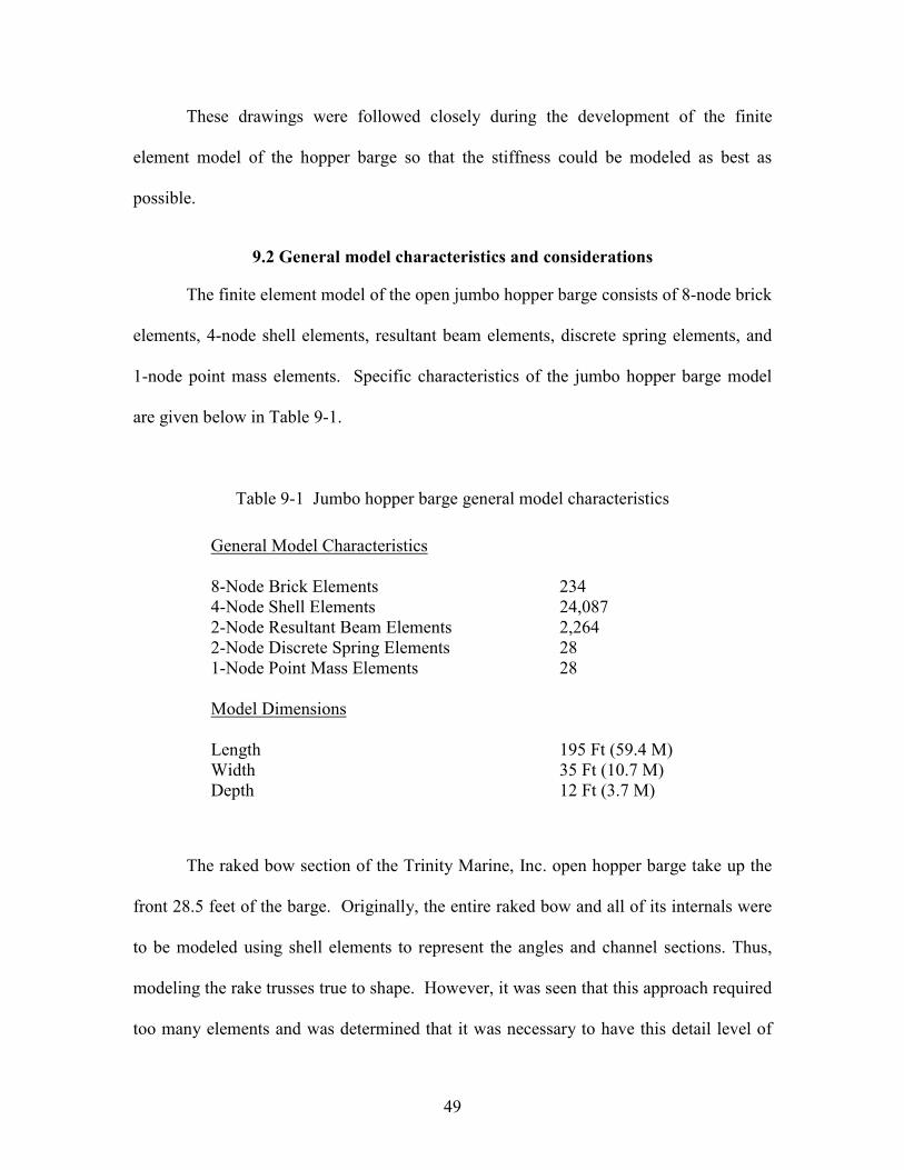
49
These drawings were followed closely during the development of the finite
element model of the hopper barge so that the stiffness could be modeled as best as
possible.
9.2 General model characteristics and considerations
The finite element model of the open jumbo hopper barge consists of 8-node brick
elements, 4-node shell elements, resultant beam elements, discrete spring elements, and
1-node point mass elements. Specific characteristics of the jumbo hopper barge model
are given below in Table 9-1.
Table 9-1 Jumbo hopper barge general model characteristics
The raked bow section of the Trinity Marine, Inc. open hopper barge take up the
front 28.5 feet of the barge. Originally, the entire raked bow and all of its internals were
to be modeled using shell elements to represent the angles and channel sections. Thus,
modeling the rake trusses true to shape. However, it was seen that this approach required
too many elements and was determined that it was necessary to have this detail level of
General Model Characteristics
8-Node Brick Elements 234 4-Node Shell Elements 24,087 2-Node Resultant Beam Elements 2,264 2-Node Discrete Spring Elements 28 1-Node Point Mass Elements 28 Model Dimensions
Length 195 Ft (59.4 M) Width 35 Ft (10.7 M) Depth 12 Ft (3.7 M)
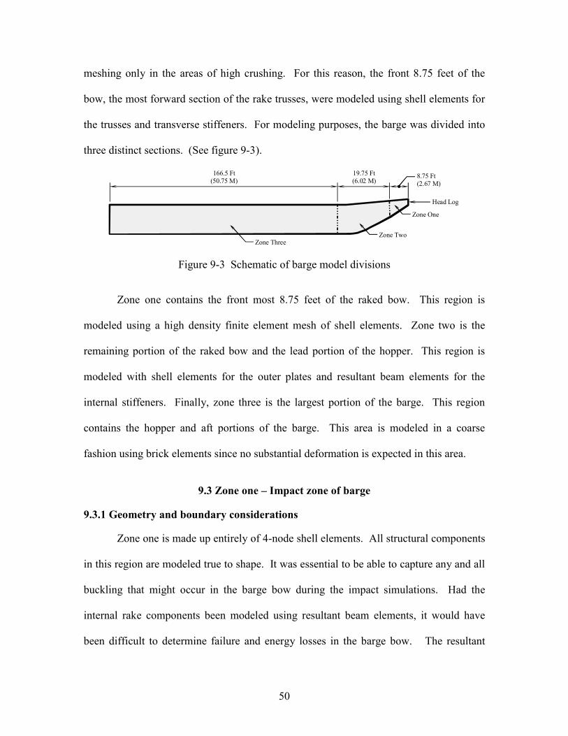
50
meshing only in the areas of high crushing. For this reason, the front 8.75 feet of the
bow, the most forward section of the rake trusses, were modeled using shell elements for
the trusses and transverse stiffeners. For modeling purposes, the barge was divided into
three distinct sections. (See figure 9-3).
Zone One
Zone TwoZone Three
8.75 Ft(2.67 M)
19.75 Ft(6.02 M)
166.5 Ft(50.75 M)
Head Log
Figure 9-3 Schematic of barge model divisions
Zone one contains the front most 8.75 feet of the raked bow. This region is
modeled using a high density finite element mesh of shell elements. Zone two is the
remaining portion of the raked bow and the lead portion of the hopper. This region is
modeled with shell elements for the outer plates and resultant beam elements for the
internal stiffeners. Finally, zone three is the largest portion of the barge. This region
contains the hopper and aft portions of the barge. This area is modeled in a coarse
fashion using brick elements since no substantial deformation is expected in this area.
9.3 Zone one – Impact zone of barge
9.3.1 Geometry and boundary considerations
Zone one is made up entirely of 4-node shell elements. All structural components
in this region are modeled true to shape. It was essential to be able to capture any and all
buckling that might occur in the barge bow during the impact simulations. Had the
internal rake components been modeled using resultant beam elements, it would have
been difficult to determine failure and energy losses in the barge bow. The resultant
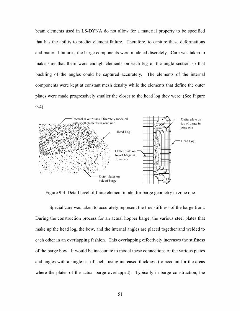
51
beam elements used in LS-DYNA do not allow for a material property to be specified
that has the ability to predict element failure. Therefore, to capture these deformations
and material failures, the barge components were modeled discretely. Care was taken to
make sure that there were enough elements on each leg of the angle section so that
buckling of the angles could be captured accurately. The elements of the internal
components were kept at constant mesh density while the elements that define the outer
plates were made progressively smaller the closer to the head log they were. (See Figure
9-4).
Head Log
Internal rake trusses, Discretely modeledwith shell elements in zone one
Outer plates onside of barge
Head Log
Outter plate ontop of barge inzone one
Outter plate ontop of barge inzone two
Figure 9-4 Detail level of finite element model for barge geometry in zone one
Special care was taken to accurately represent the true stiffness of the barge front.
During the construction process for an actual hopper barge, the various steel plates that
make up the head log, the bow, and the internal angles are placed together and welded to
each other in an overlapping fashion. This overlapping effectively increases the stiffness
of the barge bow. It would be inaccurate to model these connections of the various plates
and angles with a single set of shells using increased thickness (to account for the areas
where the plates of the actual barge overlapped). Typically in barge construction, the

52
plates are welded to one another with a butt weld that runs the length of the plate. These
welds are usually made only on one face of the plates. An illustration of this is shown in
figure 9-5 below.
Internal rake trusscomponent
Continuous fillet weld
Outer steel plate of barge
Figure 9-5 Typical welding detail for barge bow internal sections
Therefore, during crushing the plates can potentially separate from each other at
the edge where no weld is made. To achieve this in the finite element model, each plate
and angle were modeled as separate entities and were oriented such that they were almost
touching when the plates projected thickness were applied (See figure 9-6).
t2*
t1*
Shell Element Nodal Line
Shell Element Nodal Line
* Projected Element Thicknesses** Gap dimension must be greater than zero for Single Surface Contact Algorithims to Function Properly
Gap**
Figure 9-6 Illustration of shell element separations
The plates and angles were then attached to each other using a constraint in
LS-DYNA, *CONSTRAINED_SPOTWELD. This constraint is used to represent a spot weld
between two or more nodes. The spot weld constraint is a modification of the nodal rigid

53
body that incorporates the ability to impose a failure criterion to the weld. LS-DYNA
also offers a fillet weld type constraint, *CONSTRAINED_GENERALIZED_WELD_FILLET,
which is fundamentally equivalent to the spot weld constraint, except with the added
ability to specify a projected length of weld out from the specified nodal points. This
type of constraint more accurately represents the type of weld on the plates and angles of
an actual barge, however, due to continuously varying element sizes in the barge model,
the fillet weld constraints were not used since a unique weld length would have had to be
computed for each of the hundreds of welds that are present in the model. It was decided
that due to the small element size used in the outer plates, the use of spot weld constraints
at nearly each node would provide a good representation of a continuous weld. The welds
used in the model are specified to have infinite strength, thus no failure criterion was
specified. This was done because it was felt that plates would most likely fail before the
welds.
9.3.2 Material Properties
The shell elements that make up Zone one of the hopper barge were given a
piecewise linear material model with specified failure for A36 structural steel. Newer
barges are being produced with higher strength steels such as HSLA-80 that have a yield
point much higher that that of A36 structural grade steel. However, most of the barges in
the U.S. fleet are at least ten to twenty years of age. These older barges are mostly
constructed from A36 grade steels. Another motivation for using the A36 grade steel
material models for the simulation was the consideration of possibly purchasing a used
barge for the full-scale impact tests. These issues are discussed in full detail in chapter 5
of the report. The material model for the A36 steel was obtained from tests conducted at

54
the University of Florida on standard 18-inch tension coupon (Anderson 2000). The steel
model for A36 steel has an initial yield of 36 kip/in2 (2.48e+08 N/m2), a yield strain of
0.0012 and a failure strain of 0.2%. The material model was specified as the effective
stress versus effective plastic strain for LS-DYNA material number 24, *MAT-
_PIECEWISE_LINEAR_PLASTICITY. This model allows for a user defined piecewise
curve for stress versus strain as well as a yield stress and failure strain. A plot of the
stress versus strain curve used is shown below in figure 9-7.
0
10
20
30
40
50
60
70
80
90
0 0.02 0.04 0.06 0.08 0.1 0.12 0.14 0.16 0.18 0.2 0.22 0.24 0.260
0.05
0.1
0.15
0.2
0.25
0.3
0.35
0.4
True
Stre
ss (k
si)
True
Stre
ss (M
Pa)
True Strain
Figure 9-7 True stress versus true strain curve for A36 structural steel
The model also allows for the addition of strain rate effects on the material using
the Cowper Symonds model. The current simulations do not implement any strain rate
effects for the A36 steel material however since barge impact events are not high speed
impact situations.
55
9.3.3 Selection of contact entities and algorithms
During an impact event where high deformation of the head log is possible, there
is a high likelihood that some of the elements of the front internal stiffening system may
deflect enough to come into contact with one another. When members deform and
contact each other, some of the overall stiffness of the system is restored due to the
deformed parts relying on one another for support. If these internal contacts were to go
undetected, the secondary stiffness of the barge system would be underestimated.
However, due to the complexity of the system, it is extremely difficult to predict where
and when these contacts will occur. To work around this problem the contact type
*CONTACT_AUTOMATIC_SINGLE_SURFACE was defined for all of the shell elements zone
one of the barge. This type of contact definition is different from traditional contact
methods in that no contact surfaces are predefined. Instead, groups of elements are
defined which may come into contact during the simulation. The automatic single
surface contact algorithm then detects all contacts occurring for the element groups
specified. The contact surface definitions and all associations are automatically
generated by LS-DYNA (Whirley 1994). Thus by specifying all the elements of the
barge front, this allows for any part to contact any other part or multiple parts at any time
during the simulation. This contact algorithm increased the amount of time needed to
complete a simulation, however it proved to be very time efficient due to the reduced
amount of time needed to develop and utilize the barge model.
9.3.4 Conflicts with combining contact algorithms
Originally, the authors planned to use a constraint type, contact definition,
*CONTACT_TIED_NODES_TO_SURFACE, in zone one of the barge where plates and angles

56
needed to be connected together to model the welded connections. It was found however
that LS-DYNA has some compatibility issues with specifying both types of contact “tied
nodes to surface” and “automatic single surface” for the same set of shell elements. The
problems are introduced due to restrictions on the distance between the shell elements
being specified for potential contact. As stated in section 9.4.1, the tied contact interface
feature offers the use of an offset algorithm but requires that the tied members be no more
than a program specified maximum distance from one another. The automatic single
surface contact algorithm has distance restrictions as well. The single surface algorithm
requires that all elements specified not be in contact with each other at initialization. This
means that the nodes that define the surfaces must be farther apart than the summation of
half the thickness of each of the potentially contacting plates, see Figure 9-8 for a
graphical representation of the problem. If the plates are too close initially, LS-DYNA
will detect it as an initial penetration of potentially contacting elements. To try and
correct the problem, LS-DYNA will move the nodes that are initially penetrating other
surfaces away so that no contact is occurring at initialization. This results in unwanted
initial stresses in the system, which can lead to erroneous results.
Equating the offset equations for the tied method and the minimum distance
requirement for the single surface method yields the following limitation on the distance
between two surfaces when it is desired to use both single surface contact and tied
contact:
)(6.0)(5.0 1212 ttOFFSETtt +×≤≤+× (9-1)

57
t2*
t1*
Shell Element Nodal Line
Shell Element Nodal Line
* Projected element thickness** Dimension limited by Equation 9-2 for the tied contact algorithm
Offset**
a) Offset limitation for tied contact algorithm
t2*
t1*
Shell Element Nodal Line
Shell Element Nodal Line
* Projected element thickness** Dimension must be greater than t1/2 + t2/2 for the single surface contact algorithm
Offset**
b) Offset limitation for single surface contact algorithm
Figure 9-8 Shell element offset limitations
Due to the small thickness of the shell elements that would need to have both
contact definitions imposed on them, the tolerance of the allowable distance between
them was extremely small. In the case shown below, the distances between both sides of
the plates have to be setup with zero error for these contact definitions to work properly
with one another.
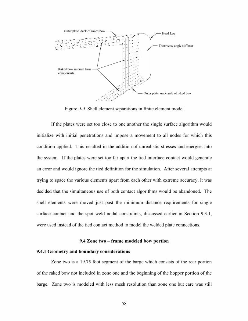
58
Head Log
Transverse angle stiffener
Outer plate, underside of raked bow
Outer plate, deck of raked bow
Raked bow internal trusscomponents
Figure 9-9 Shell element separations in finite element model
If the plates were set too close to one another the single surface algorithm would
initialize with initial penetrations and impose a movement to all nodes for which this
condition applied. This resulted in the addition of unrealistic stresses and energies into
the system. If the plates were set too far apart the tied interface contact would generate
an error and would ignore the tied definition for the simulation. After several attempts at
trying to space the various elements apart from each other with extreme accuracy, it was
decided that the simultaneous use of both contact algorithms would be abandoned. The
shell elements were moved just past the minimum distance requirements for single
surface contact and the spot weld nodal constraints, discussed earlier in Section 9.3.1,
were used instead of the tied contact method to model the welded plate connections.
9.4 Zone two – frame modeled bow portion
9.4.1 Geometry and boundary considerations
Zone two is a 19.75 foot segment of the barge which consists of the rear portion
of the raked bow not included in zone one and the beginning of the hopper portion of the
barge. Zone two is modeled with less mesh resolution than zone one but care was still
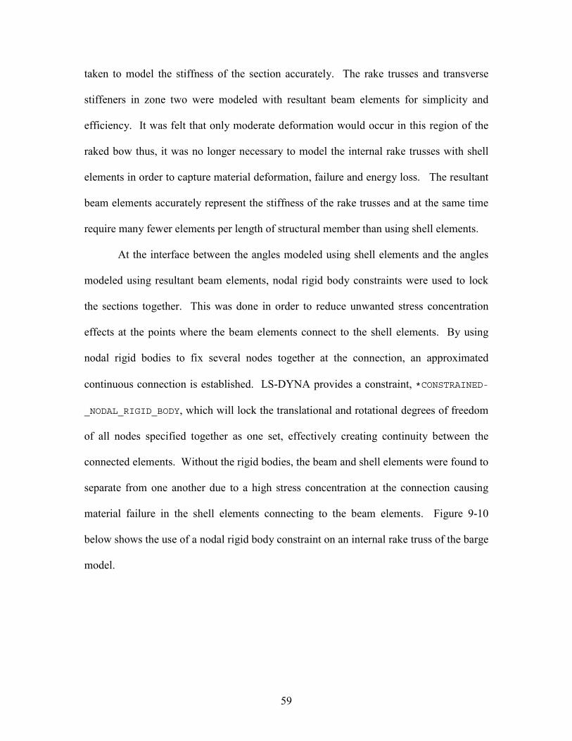
59
taken to model the stiffness of the section accurately. The rake trusses and transverse
stiffeners in zone two were modeled with resultant beam elements for simplicity and
efficiency. It was felt that only moderate deformation would occur in this region of the
raked bow thus, it was no longer necessary to model the internal rake trusses with shell
elements in order to capture material deformation, failure and energy loss. The resultant
beam elements accurately represent the stiffness of the rake trusses and at the same time
require many fewer elements per length of structural member than using shell elements.
At the interface between the angles modeled using shell elements and the angles
modeled using resultant beam elements, nodal rigid body constraints were used to lock
the sections together. This was done in order to reduce unwanted stress concentration
effects at the points where the beam elements connect to the shell elements. By using
nodal rigid bodies to fix several nodes together at the connection, an approximated
continuous connection is established. LS-DYNA provides a constraint, *CONSTRAINED-
_NODAL_RIGID_BODY, which will lock the translational and rotational degrees of freedom
of all nodes specified together as one set, effectively creating continuity between the
connected elements. Without the rigid bodies, the beam and shell elements were found to
separate from one another due to a high stress concentration at the connection causing
material failure in the shell elements connecting to the beam elements. Figure 9-10
below shows the use of a nodal rigid body constraint on an internal rake truss of the barge
model.
60
Zone one, discretely modeledinternal rake truss elements
Zone two, approximatedinternal rake truss elements
Nodal rigid body constraint usedto attach zone one and zone twoelements to on another
Nodal rigid body constraint usedto attach zone one and zone twoelements to on another
Figure 9-10 Nodal rigid body constraints on internal rake trusses
The outer deck and sidewall plates of zone two are modeled using shell elements
like the outer plates in zone one. The shell elements in zone two remain the same size
throughout the section wherever possible. In some areas of transition, the element size
decreases but in all areas of flat or curved plate, the element size is not varied. The outer
plates were not connected to the resultant beam rake trusses using the same spot weld
constraints that were used in zone one. Instead, a form of a constrained contact definition
was used to attach the outer plates and the internal trusses. The generalized constraint
type contact definition, *CONTACT_TIED_NODES_TO_SURFACE, allows a group of nodes to
be specified as being “tied” in all degrees of freedom to a specified contact surface. In
general, LS-DYNA requires that the nodes to be constrained lie in the plane of the
constraining surface. LS-DYNA also permits the use of an OFFSET option for the tied
contact constraint. By specifying the offset option for the tied contact algorithm,
LS-DYNA changes it formulation of the contact from a constraint method to a penalty-
based method. This penalty-based formulation allows the tied nodes to be slightly
separated from the surface to which they are tied. If the offset option is not set and the
61
nodes specified do not lie in the plane of the constraining surface, the nodes are projected
onto the surface upon initialization. This nodal projection causes unrealistic stresses in
the elements connected to the nodes that are moved. Therefore, to ensure accurate
results, all nodal projections at the initialization stage of the simulation were sought be
avoided. This offset method is constrained only in that the nodes and surface must be
close enough to one another. The allowable separation is defined in terms of the
projected thickness of the surfaces and or nodes being tied together. Given below is the
equation that is used to define the maximum amount of initial distance between two tied
surfaces or nodes:
)(6.0 nodemasterofthicknessnodeslaveofthicknessOFFSET +×≤ (9-2)
For node to surface constraints involving nodes of discrete and resultant beam elements
tied to surfaces of shell elements, it was found that LS-DYNA treats the thickness of the
beam element nodes as zero. If the nodes specified are farther away from the master
segment than the maximum allowable offset value, a warning message is displayed at
initialization and the tied interface for these nodes is ignored in the simulation.
9.4.2 Material Properties
The outer plates of the barge in zone two are modeled using the same material
properties as the plates in zone one. The material is A36 steel and is modeled using a
piecewise linear stress versus strain curve with failure. The material model is explained
in detail in section 9.3.2. The resultant beam elements used for the internal frame
elements of zone two were modeled using a simple linear elastic material model.
Originally, the beam elements were to be modeled using the same material model as the
shell elements. However it was found that LS-DYNA would not allow the beam
62
elements to have a material model that incorporated failure, therefore a new material
model had to be chosen. A simple linear elastic material model proved to be the best
option since it was not anticipated that the material in zone two would undergo any
inelastic deformations. The LS-DYNA material model, *MAT_LINEAR_ELASTIC is the
general model for elastic, perfectly plastic material modeling. The model only requires a
material mass density, an elastic modulus and a Poisson’s ratio. The values used were,
15.217 lbf-sec2/ft4 (7860 kg/m3), 29000 kip/in2 (2.0e+11 N/m2) and 0.33 respectively.
9.5 Zone three – Rear Hopper
9.5.1 Geometry and boundary considerations
The remaining 166.5 feet of the jumbo hopper barge was modeled using large
8-node brick elements. The meshing in this region is extremely coarse, as no buckling
will occur in this region. The rear portion of the barge was modeled not only for
visualization purposes but also to represent the total mass inertia of the barge. It would
have been inaccurate to simply model only the front portions of the barge and attach
point masses to that section to approximate the total weight. By modeling the whole
barge, the correct mass and inertial properties are achieved. Brick elements where
arranged as a solid block that measured 166.5 feet long by 35 feet wide and 12 feet deep.
This rear section was attached to the shell and beam element front rake section through a
nodal rigid body constraint. This constraint attached all the nodes along the connecting
interface together in one rigid body connection.
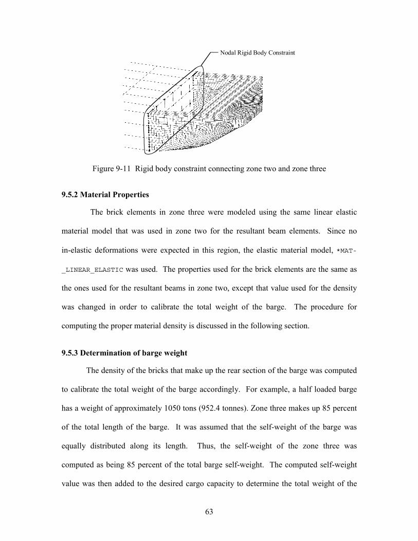
63
Nodal Rigid Body Constraint
Figure 9-11 Rigid body constraint connecting zone two and zone three
9.5.2 Material Properties
The brick elements in zone three were modeled using the same linear elastic
material model that was used in zone two for the resultant beam elements. Since no
in-elastic deformations were expected in this region, the elastic material model, *MAT-
_LINEAR_ELASTIC was used. The properties used for the brick elements are the same as
the ones used for the resultant beams in zone two, except that value used for the density
was changed in order to calibrate the total weight of the barge. The procedure for
computing the proper material density is discussed in the following section.
9.5.3 Determination of barge weight
The density of the bricks that make up the rear section of the barge was computed
to calibrate the total weight of the barge accordingly. For example, a half loaded barge
has a weight of approximately 1050 tons (952.4 tonnes). Zone three makes up 85 percent
of the total length of the barge. It was assumed that the self-weight of the barge was
equally distributed along its length. Thus, the self-weight of the zone three was
computed as being 85 percent of the total barge self-weight. The computed self-weight
value was then added to the desired cargo capacity to determine the total weight of the
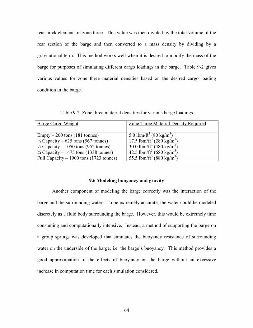
64
rear brick elements in zone three. This value was then divided by the total volume of the
rear section of the barge and then converted to a mass density by dividing by a
gravitational term. This method works well when it is desired to modify the mass of the
barge for purposes of simulating different cargo loadings in the barge. Table 9-2 gives
various values for zone three material densities based on the desired cargo loading
condition in the barge.
Table 9-2 Zone three material densities for various barge loadings
Barge Cargo Weight Zone Three Material Density Required
Empty – 200 tons (181 tonnes) 5.0 lbm/ft3 (80 kg/m3) ¼ Capacity – 625 tons (567 tonnes) 17.5 lbm/ft3 (280 kg/m3) ½ Capacity – 1050 tons (952 tonnes) 30.0 lbm/ft3 (480 kg/m3) ¾ Capacity – 1475 tons (1338 tonnes) 42.5 lbm/ft3 (680 kg/m3) Full Capacity – 1900 tons (1723 tonnes) 55.5 lbm/ft3 (880 kg/m3)
9.6 Modeling buoyancy and gravity
Another component of modeling the barge correctly was the interaction of the
barge and the surrounding water. To be extremely accurate, the water could be modeled
discretely as a fluid body surrounding the barge. However, this would be extremely time
consuming and computationally intensive. Instead, a method of supporting the barge on
a group springs was developed that simulates the buoyancy resistance of surrounding
water on the underside of the barge, i.e. the barge’s buoyancy. This method provides a
good approximation of the effects of buoyancy on the barge without an excessive
increase in computation time for each simulation considered.
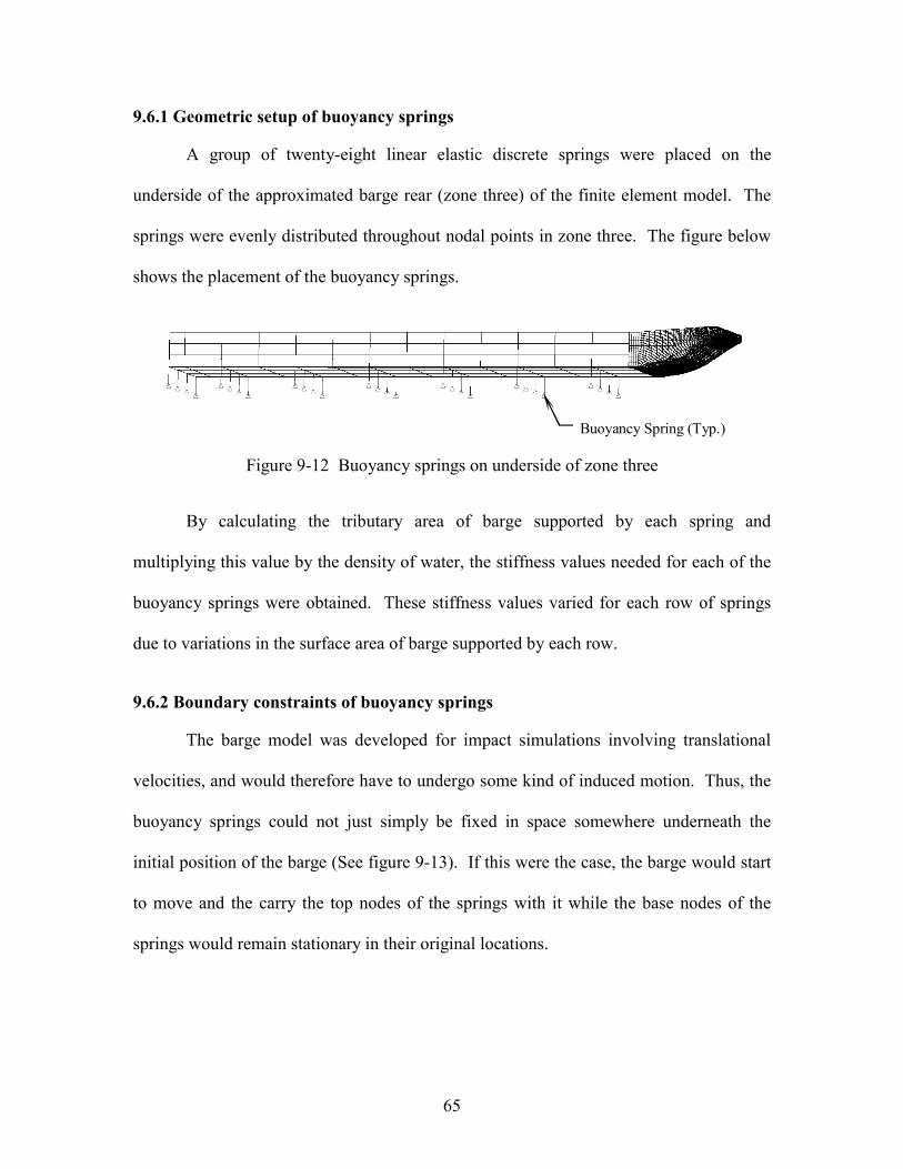
65
9.6.1 Geometric setup of buoyancy springs
A group of twenty-eight linear elastic discrete springs were placed on the
underside of the approximated barge rear (zone three) of the finite element model. The
springs were evenly distributed throughout nodal points in zone three. The figure below
shows the placement of the buoyancy springs.
Buoyancy Spring (Typ.)
Figure 9-12 Buoyancy springs on underside of zone three
By calculating the tributary area of barge supported by each spring and
multiplying this value by the density of water, the stiffness values needed for each of the
buoyancy springs were obtained. These stiffness values varied for each row of springs
due to variations in the surface area of barge supported by each row.
9.6.2 Boundary constraints of buoyancy springs
The barge model was developed for impact simulations involving translational
velocities, and would therefore have to undergo some kind of induced motion. Thus, the
buoyancy springs could not just simply be fixed in space somewhere underneath the
initial position of the barge (See figure 9-13). If this were the case, the barge would start
to move and the carry the top nodes of the springs with it while the base nodes of the
springs would remain stationary in their original locations.
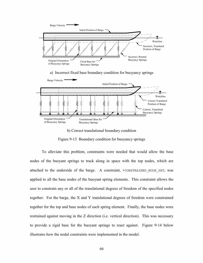
66
Original Orientationof Buoyancy Springs
Fixed Base forBuoyancy Springs
Waterline
Incorrect, RotatedBuoyancy Springs
Barge Velocity
Initial Position of Barge
Incorrect, TranslatedPosition of Barge
a) Incorrect fixed base boundary condition for buoyancy springs
Waterline
Correct, TranslatedBuoyancy Springs
Barge VelocityInitial Position of Barge
Correct TranslatedPosition of Barge
Translational Base forBuoyancy Springs
Original Orientationof Buoyancy Springs
b) Correct translational boundary condition
Figure 9-13 Boundary condition for buoyancy springs
To alleviate this problem, constraints were needed that would allow the base
nodes of the buoyant springs to track along in space with the top nodes, which are
attached to the underside of the barge. A constraint, *CONSTRAINED_NODE_SET, was
applied to all the base nodes of the buoyant spring elements. This constraint allows the
user to constrain any or all of the translational degrees of freedom of the specified nodes
together. For the barge, the X and Y translational degrees of freedom were constrained
together for the top and base nodes of each spring element. Finally, the base nodes were
restrained against moving in the Z direction (i.e. vertical direction). This was necessary
to provide a rigid base for the buoyant springs to react against. Figure 9-14 below
illustrates how the nodal constraints were implemented in the model.

67
X1
Z1
Y1
X2
Z2
Y2
Buoyancy Spring
Top Node: Attachedto Barge Bottom
Base Node: Rigidly Fixedin the Z Direction
1-Node Point Element
Nodal Constraints
X1 and X2 constrained to move together
Y1 and Y2 constrained to move together
Z1 free from constraints
Z2 constrained from motion
Figure 9-14 Schematic of spring constraint layout
In addition to the constrained node sets, point mass elements had to be added to
the base nodes of the springs (see Figure 9-14 above). LS-DYNA will not allow discrete
spring elements to be attached to massless nodes. Thus, the point masses were added to
the base nodes so that LS-DYNA would accept the buoyant springs. The weight of the
masses added were 22 pounds (98 Newtons) each, thus adding to the total weight of the
barge, 616 pounds (2744 Newtons). This added weight (mass) is negligible in
comparison to the weight (mass) of the empty barge, which is approximately 200 tons
(181.4 tonnes). The spring masses become even more insignificant when considering the
weight of the barge cargo load.
9.6.3 Determination of spring offsets for buoyancy springs
Gravitational force was also added to the finite element model of the hopper barge
to work in conjunction with the buoyant springs. This gravitational force is applied to
both the barge and the pier models and is present in the impact simulations. The addition
of gravity into the model of the hopper barge presented a special problem. The buoyant
springs that were added to the model to simulate buoyancy effects were not calibrated to
resist gravity, instead they were designed to simulate the effects of the surrounding water

68
on the barge if the barge were to translate vertically with respect to their initial positions.
The buoyancy springs had to be calibrated to handle the gravitational forces that were
introduced into the model. There are two methods available for calibrating the buoyant
springs to handle the gravitational forces. In the first method, gravity would be applied to
the model without any pre-compression added to the buoyant springs. This addition of
gravity will cause the barge to “draft” or sink causing the buoyant springs to develop
resistance to the gravitational forces of the barge. Once settled, the draft of the barge is
measured. Then, the barge model is repositioned such that after it has settled due to the
addition of gravity, it lies in the correct orientation for impact (see Figure 9-15). The
second method for applying gravitational forces to the model involves adding pre-
compression to the buoyant springs. Using the draft measurements from method one and
the spring stiffness values, spring force values can be computed for each buoyant spring
in the barge model. These force values are added into the model as pre-compression
forces in the buoyant springs. The advantage to this method over method one is that
when the gravitational forces are introduced into the model, the barge does not change its
vertical position (see Figure 9-15).

69
Buoyancy SpringsRigid Base forBuoyancy Springs
Position of Barge BeforeApplication of Gravitational Force
Settled Position of Barge
Impact Test Pier
Waterline
Gravitational Force
a) Method One: No spring pre-compression
Pre-CompressedBuoyancy SpringsRigid Base for
Buoyancy Springs
Gravitational Force
Initial and Settled Position of Barge
Waterline
Impact Test Pier
b) Method Two: Pre-compression in buoyancy springs
Figure 9-15 Methods of gravitational force application
The second method using spring pre-compression was used in the barge model.
LS-DYNA provides an option for discrete spring elements that allows for specifying an
initial compression or tension. LS-DYNA refers to this as an “initial offset” at time zero
in the model simulation. This process was done in an iterative fashion until the barge did
not displace upon initialization of the gravitational forces. By using method two, it was
possible to apply gravity to the entire model at the start of the simulation. Unlike method
one, method two required no initial settling of the barge model before to each simulation.

70
CHAPTER 10 DEVELOPMENT OF FINITE ELEMENT MODELS
FOR CAUSEWAY PIERS
10.1 Description of causeway support piers
Finite element models of the causeway piers that were chosen for impact testing
had to be developed in order to conduct simulations of the impact events. Finite element
models for support pier-1 and pier-3 are shown below in the elevation illustration of the
causeway (Figure 10-1).
To: Saint George Island, SouthTo: Cat Point, North
Center-Line, Main ICWW ChannelTimber Bridge Fender Wales
Continuous Steel Girder SpanSingle Concrete AASHTO Girder Spans
MHW line
End ofBridge
Barrier IslandMud line
Pier-3Pier-1
Pier-1Pier-3
Figure 10-1 Elevation of Saint George Island Causeway Bridge
The reasons for choosing pier-1 and pier-3 have been described in Chapter 3.
Pier-1 is a main impact pier adjacent to the channel, while pier-3 is a secondary pier
located 396 ft from the centerline of the 250 ft wide channel pass. Both piers are cast-in-
place reinforced concrete structures but differ both in impact resistance strength and in
the type of piles utilized. In order to develop accurate models of each pier, copies of the
record drawings for the causeway were obtained. These drawings were followed closely
in developing the geometry of the pier models.
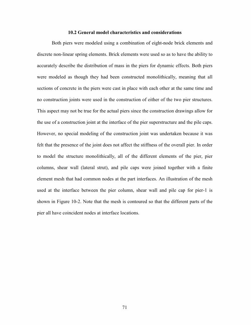
71
10.2 General model characteristics and considerations
Both piers were modeled using a combination of eight-node brick elements and
discrete non-linear spring elements. Brick elements were used so as to have the ability to
accurately describe the distribution of mass in the piers for dynamic effects. Both piers
were modeled as though they had been constructed monolithically, meaning that all
sections of concrete in the piers were cast in place with each other at the same time and
no construction joints were used in the construction of either of the two pier structures.
This aspect may not be true for the actual piers since the construction drawings allow for
the use of a construction joint at the interface of the pier superstructure and the pile caps.
However, no special modeling of the construction joint was undertaken because it was
felt that the presence of the joint does not affect the stiffness of the overall pier. In order
to model the structure monolithically, all of the different elements of the pier, pier
columns, shear wall (lateral strut), and pile caps were joined together with a finite
element mesh that had common nodes at the part interfaces. An illustration of the mesh
used at the interface between the pier column, shear wall and pile cap for pier-1 is
shown in Figure 10-2. Note that the mesh is contoured so that the different parts of the
pier all have coincident nodes at interface locations.
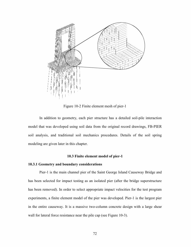
72
Figure 10-2 Finite element mesh of pier-1
In addition to geometry, each pier structure has a detailed soil-pile interaction
model that was developed using soil data from the original record drawings, FB-PIER
soil analysis, and traditional soil mechanics procedures. Details of the soil spring
modeling are given later in this chapter.
10.3 Finite element model of pier-1
10.3.1 Geometry and boundary considerations
Pier-1 is the main channel pier of the Saint George Island Causeway Bridge and
has been selected for impact testing as an isolated pier (after the bridge superstructure
has been removed). In order to select appropriate impact velocities for the test program
experiments, a finite element model of the pier was developed. Pier-1 is the largest pier
in the entire causeway. It is a massive two-column concrete design with a large shear
wall for lateral force resistance near the pile cap (see Figure 10-3).
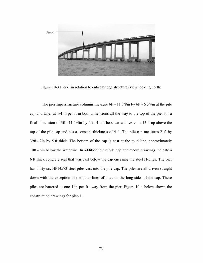
73
Pier-1
Figure 10-3 Pier-1 in relation to entire bridge structure (view looking north)
The pier superstructure columns measure 6ft - 11 7/8in by 6ft - 6 3/4in at the pile
cap and taper at 1/4 in per ft in both dimensions all the way to the top of the pier for a
final dimension of 3ft - 11 1/4in by 4ft - 4in. The shear wall extends 15 ft up above the
top of the pile cap and has a constant thickness of 4 ft. The pile cap measures 21ft by
39ft - 2in by 5 ft thick. The bottom of the cap is cast at the mud line, approximately
10ft - 6in below the waterline. In addition to the pile cap, the record drawings indicate a
6 ft thick concrete seal that was cast below the cap encasing the steel H-piles. The pier
has thirty-six HP14x73 steel piles cast into the pile cap. The piles are all driven straight
down with the exception of the outer lines of piles on the long sides of the cap. These
piles are battered at one 1 in per ft away from the pier. Figure 10-4 below shows the
construction drawings for pier-1.
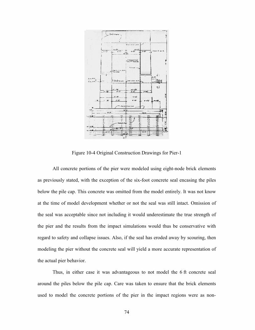
74
Figure 10-4 Original Construction Drawings for Pier-1
All concrete portions of the pier were modeled using eight-node brick elements
as previously stated, with the exception of the six-foot concrete seal encasing the piles
below the pile cap. This concrete was omitted from the model entirely. It was not know
at the time of model development whether or not the seal was still intact. Omission of
the seal was acceptable since not including it would underestimate the true strength of
the pier and the results from the impact simulations would thus be conservative with
regard to safety and collapse issues. Also, if the seal has eroded away by scouring, then
modeling the pier without the concrete seal will yield a more accurate representation of
the actual pier behavior.
Thus, in either case it was advantageous to not model the 6 ft concrete seal
around the piles below the pile cap. Care was taken to ensure that the brick elements
used to model the concrete portions of the pier in the impact regions were as non-

75
distorted as possible. This was done to minimize error in the model results. Severely
skewed and distorted elements have a tendency to produce modeling errors and develop
hourglass energy modes. However, such problems can be generally be eliminated by
using carefully graded brick meshes. The steel H-piles were modeled using “resultant
beam” elements. These elements were extended into the under side of the pile cap to
simulate the embedment length of the true piles. Each pile consisted of a number of
beam elements, each four feet in length and having the cross sectional properties of the
HP14x73 steel piles (see Figure 10-5).
Figure 10-5 Final Finite Element Model of Pier-1
10.3.2 Material properties
Extremely accurate modeling of reinforced concrete requires a complex material
model that accounts for non-linear concrete and steel behavior, cracking, and pressure
dependencies. Examples of complex material models used for modeling concrete are the
Druker-Prager and the Mohr-Coulomb models. Since the proposed impact testing will be
non-destructive in nature, the use of complex material models was not warranted. It was

76
sufficient for purposes of accurately representing the pier stiffness and inertial
resistance, to model the concrete material using a simpler linear elastic material model.
The material model used in the LS-DYNA simulations was, *MAT_LINEAR_ELASTIC.
This material model provides accurate stiffness representation for materials exhibiting
elastic behavior. Stresses developed in the pier model from the barge impact event were
analyzed to ensure that they remained within the elastic range of the concrete material.
Table 10-1 below shows the properties used for the linear elastic material model used for
the concrete in pier-1.
Table 10-1 Material values used for linear elastic model of concrete
Weight Density 150 lb/ft3 ( 23563 N/m3 )Modulus of Elasticity 4030 lb/ft2 ( 2.7786E+10 N/m2 )Poisson’s Ratio 0.15
A linear elastic material model was also used for the resultant beam elements
that represent the steel H-piles of pier-1. These beam elements were modeled using the
same material model as the resultant beams in zone-2 of the hopper barge model
discussed in Section 9.5.2.
10.3.3 Soil-pile interaction model
To properly represent the bridge pier’s response to a dynamic lateral impact
event, it was necessary to model the resistance of the surrounding soil to movement of
the bridge piles. Traditional methods of numerical modeling were used to
mathematically approximate the interaction between the piles and the soil. At each nodal
location (at 4 ft vertical intervals) three discrete spring elements were used to represent
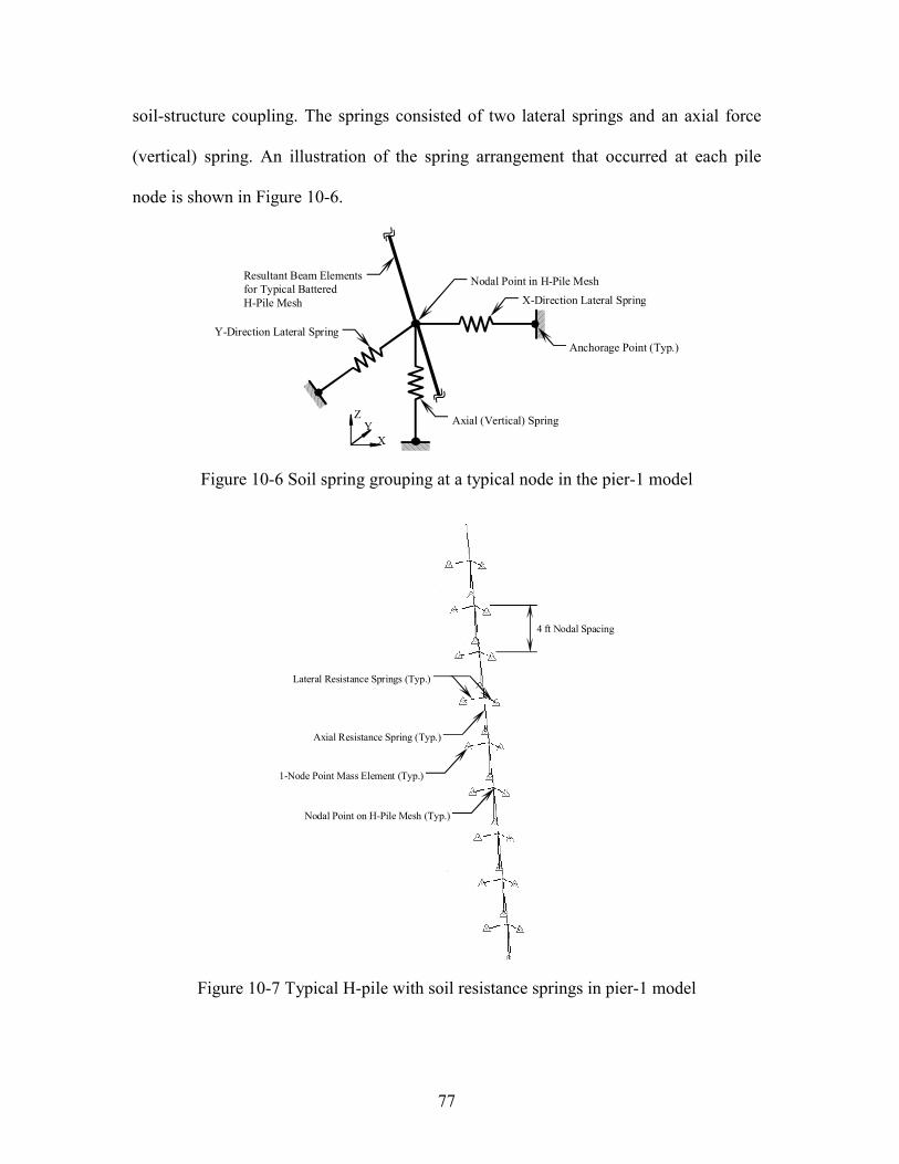
77
soil-structure coupling. The springs consisted of two lateral springs and an axial force
(vertical) spring. An illustration of the spring arrangement that occurred at each pile
node is shown in Figure 10-6.
X
ZY Axial (Vertical) Spring
X-Direction Lateral Spring
Y-Direction Lateral Spring
Resultant Beam Elementsfor Typical BatteredH-Pile Mesh
Nodal Point in H-Pile Mesh
Anchorage Point (Typ.)
Figure 10-6 Soil spring grouping at a typical node in the pier-1 model
Lateral Resistance Springs (Typ.)
Axial Resistance Spring (Typ.)
1-Node Point Mass Element (Typ.)
Nodal Point on H-Pile Mesh (Typ.)
4 ft Nodal Spacing
Figure 10-7 Typical H-pile with soil resistance springs in pier-1 model
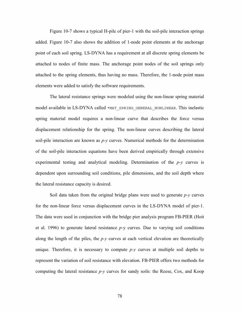
78
Figure 10-7 shows a typical H-pile of pier-1 with the soil-pile interaction springs
added. Figure 10-7 also shows the addition of 1-node point elements at the anchorage
point of each soil spring. LS-DYNA has a requirement at all discrete spring elements be
attached to nodes of finite mass. The anchorage point nodes of the soil springs only
attached to the spring elements, thus having no mass. Therefore, the 1-node point mass
elements were added to satisfy the software requirements.
The lateral resistance springs were modeled using the non-linear spring material
model available in LS-DYNA called *MAT_SPRING_GENERAL_NONLINEAR. This inelastic
spring material model requires a non-linear curve that describes the force versus
displacement relationship for the spring. The non-linear curves describing the lateral
soil-pile interaction are known as p-y curves. Numerical methods for the determination
of the soil-pile interaction equations have been derived empirically through extensive
experimental testing and analytical modeling. Determination of the p-y curves is
dependent upon surrounding soil conditions, pile dimensions, and the soil depth where
the lateral resistance capacity is desired.
Soil data taken from the original bridge plans were used to generate p-y curves
for the non-linear force versus displacement curves in the LS-DYNA model of pier-1.
The data were used in conjunction with the bridge pier analysis program FB-PIER (Hoit
et al. 1996) to generate lateral resistance p-y curves. Due to varying soil conditions
along the length of the piles, the p-y curves at each vertical elevation are theoretically
unique. Therefore, it is necessary to compute p-y curves at multiple soil depths to
represent the variation of soil resistance with elevation. FB-PIER offers two methods for
computing the lateral resistance p-y curves for sandy soils: the Reese, Cox, and Koop
79
method and the O’Neill method. The Reese, Cox, and Koop method is the older of the
two, developed in 1974, while the O’Neill method is more current, having been
developed in 1984. Both methods require the user to specify the soil properties φ
(internal angle of friction), γ (soil unit weight), and soil depth at the analysis point. φ is
computed by FB-PIER from the soil data while the unit weight used was an average
value for sandy soils. The Reese, Cox, and Koop method yields soil springs with lower
stiffness (resulting in larger pile displacements) than the O’Neill method. For the impact
simulations of Phase I of this project, the main focus was on studying the dynamic
interaction between the barge and the pier. This interaction is significantly affected by
displacement of the pier during impact and thus, the Reese, Cox, and Koop method, was
chosen for the calculation of the p-y curves in the LS-DYNA model. Future simulations
will be conducted using both methods of soil-pile interaction to provide both upper and
lower bounds on the pier response during impact.
FB-PIER allows the user to represent the soil as multiple layers with each layer
having a unique set of soil properties. In this study, the soil was divided into eight
different layers. Two p-y curves were generated by FB-PIER for each layer of soil in the
model. The curves corresponded to the elevations at the top and bottom of each soil
layer. Since FB-PIER does not produce curve values midway through the layers, the
curves were assumed to vary linearly through each layer of soil. Since the lateral
resistance springs were placed at depth increments of four feet in the LS-DYNA model
of pier-1, it was desired that unique p-y curves be generated for each spring group. A
MathCad worksheet was created that linearly interpolated p-y curve data from the data
produced by FB-PIER.
80
The Reese, Cox, and Koop p-y curve model reaches a yield point at which the
soil offers no further lateral resistance. This flat (plastic) portion of the p-y curve
presented a problem with LS-DYNA. LS-DYNA does not permit discrete spring
elements to be defined with a zero tangent modulus as occurs in the plastic region of the
p-y curves. Also, the p-y curves generated by FB-PIER indicated plastic behavior
beyond when pier displacements exceed approximately 1.1 inches. LS-DYNA computes
the stiffness of non-linear spring elements as zero for any displacement that exceeds the
displacement of the final point in the curve used for that specific spring. Since pier
displacements greater that 1.1 inches were expected in the impact simulations, the p-y
curves were extended to accommodate a displacement of up to 12 inches and the plastic
portions of the curves were given a very small positive slope. For each curve, the slope
was computed to be one tenth of a percent (0.1%) of the initial slope.
Modeling of barge impacts on bridge piers also requires additional
considerations due to the cyclic dynamic nature of most impact events. Soil models for
lateral stiffness such as the Reese, Cox, and Koop and O’Neill methods provide non-
linear load vs. deflection relationships for the soil in the undisturbed case. However,
when soil is displaced in an oscillatory fashion, as in a dynamic situation with load
reversals, it is subjected to multiple cycles of loading and cannot be treated as
“undisturbed” through the entire duration of the analysis. Instead, the use of a gap
formulation, as illustrated in Figure 10-8, should be used to represent such behavior.
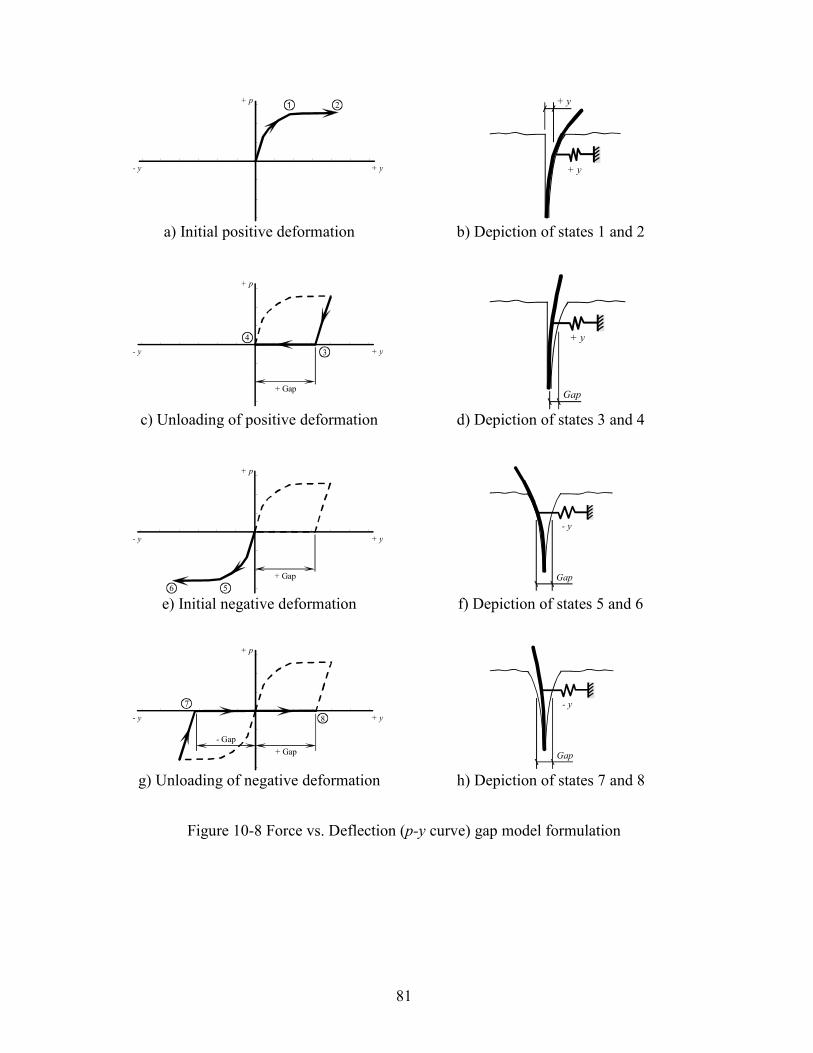
81
1 2+ p
+ y- y
3
4
+ Gap
+ p
+ y- y
56+ Gap
+ p
+ y- y
7
8
+ Gap- Gap
+ p
+ y- y
+ y
+ y
Gap
+ y
Gap
- y
Gap
- y
a) Initial positive deformation b) Depiction of states 1 and 2
c) Unloading of positive deformation d) Depiction of states 3 and 4
e) Initial negative deformation f) Depiction of states 5 and 6
g) Unloading of negative deformation h) Depiction of states 7 and 8
Figure 10-8 Force vs. Deflection (p-y curve) gap model formulation

82
9 10
+ Gap- Gap
+ p
+ y- y
Gap
+ y
1112
+ Gap- Gap
+ p
+ y- y
Gap
+ y
1314
+ Gap- Gap
+ p
+ y- y
Gap
- y
i) Secondary positive deformation j) Depiction of states 9 and 10
k) Unloading of positive deformation l) Depiction of states 11 and 12
m) Secondary negative deformation n) Depiction of states 13 and 14
Figure 10-8 Force vs. Deflection (p-y curve) gap model formulation
This model tracks elastic and plastic (permanent) components of deformation
separately in each direction (+y and –y) as cyclic loading occurs. As load is initially
applied in the +y direction and displacement of the undisturbed soil occurs, the soil
resistance is described by the undisturbed Reese, Cox, and Koop p-y curve. Between
states 1 and 2, the soil behaves in a plastic manner undergoing permanent deformation at
nearly constant load. Upon load reversal, the soil unloads along an elastic curve—having
the same slope as the initial slope of the p-y curve—from states 2 to 3 until the soil

83
resistance is zero (at state 3). At this stage, it is assumed that due to permanent
deformation, the soil in the +y direction has formed a gap.
As load application in the –y direction continues, the pile is free to move without
resistance (states 3 to 4) until it meets the undisturbed soil in the –y direction. At this
stage, the soil once again loads along an undisturbed soil p-y curve (from states 4 to 5)
because the soil on the –y side of the pile is assumed to have been unaffected by the
previous loading in the +y direction. From states 5 to 6, plastic deformation in the –y
direction occurs. When the applied load once again reverses direction, the soil unloads
elastically from state 6 to 7 until the soil resistance is zero. At this state, permanent
deformation has occurred in both the –y and +y directions and the total gap size is the
sum of the gaps in each of these directions.
Starting at state 7, if load is applied in the +y direction, the pile will move
through the entire gap width before soil resistance is once again generated at state 8. At
this state, the soil loads along the same curve (states 8 to 9) that it previous unloaded
along (states 2 to 3). When the load level reaches the previous yield point at state 9,
plastic deformation once again occurs. The next time the applied load reverses, the soil
unloads elastically from states 10 to 11. With continued –y loading, the pile will traverse
the entire gap and will move from states 11 to 12 without resistance. At state 12, elastic
loading occurs (from states 12 to 13) until the previous yield point is reached at 13. With
continued loading, the soil will undergo –y plastic deformation until once again the load
reverses at state 14 and the process continues in this same manner.
Nonlinear discrete spring elements were used in the LS-DYNA simulations to
model the gap formation process described above. Failure to account for permanent

84
deformations in the soil (i.e. formation of gaps) can produce erroneous predictions of
soil and pier displacements and therefore incorrect predictions of contact force between
the barge and pier. By using nonlinear springs to represent gap formation, the energy
dissipation associated with the inelastic response of the soil is incorporated into the
simulation and realistic predictions of barge-pier contact force are produced.
In addition to the springs representing lateral soil resistance, springs were also
added to simulate the skin friction of the pile face with the surrounding soil. Due to this
skin friction, a pile will shed axial load down its length, distributing the load carried by
the pile into the soil. Without the axial springs, the pile would have resistance only at the
tip, and the entire load carried by the pile would be transmitted to the tip, causing an
inaccurate representation of the behavior of the pile. To avoid this problem, vertical
(axial) soil springs are used. These springs are non-linear like the lateral soil resistance
springs but exhibit a force versus displacement relationship known as a T-Z curve. T-Z
curves also vary with changing soil conditions much like the p-y curves for lateral soil
resistance. The T-Z curves added to the LS-DYNA model were computed using
formulas based upon soil data taken from the bridge plans. The formulas were
implemented in a MathCad worksheet that was used to generate curve information at
four-foot intervals down the length of the piles.
The axial springs were modeled using the same non-linear discrete spring
element model that was used for the p-y curves. Also, the T-Z curves approximate a soil
yield point and exhibit a plastic region much like the p-y curves. The added
displacement length of the axial springs was approximated in the same fashion, using a
ten percent value of the original slope, as the lateral resistance springs. The axial springs
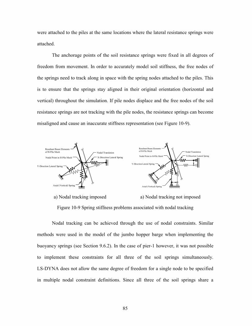
85
were attached to the piles at the same locations where the lateral resistance springs were
attached.
The anchorage points of the soil resistance springs were fixed in all degrees of
freedom from movement. In order to accurately model soil stiffness, the free nodes of
the springs need to track along in space with the spring nodes attached to the piles. This
is to ensure that the springs stay aligned in their original orientation (horizontal and
vertical) throughout the simulation. If pile nodes displace and the free nodes of the soil
resistance springs are not tracking with the pile nodes, the resistance springs can become
misaligned and cause an inaccurate stiffness representation (see Figure 10-9).
Axial (Vertical) Spring
X-Direction Lateral Spring
Y-Direction Lateral Spring
Resultant Beam Elementsof H-Pile Mesh
Nodal Point in H-Pile Mesh
Nodal Translation
Axial (Vertical) Spring
X-Direction Lateral Spring
Y-Direction Lateral Spring
Resultant Beam Elementsof H-Pile Mesh
Nodal Point in H-Pile Mesh
Nodal Translation
a) Nodal tracking imposed a) Nodal tracking not imposed
Figure 10-9 Spring stiffness problems associated with nodal tracking
Nodal tracking can be achieved through the use of nodal constraints. Similar
methods were used in the model of the jumbo hopper barge when implementing the
buoyancy springs (see Section 9.6.2). In the case of pier-1 however, it was not possible
to implement these constraints for all three of the soil springs simultaneously.
LS-DYNA does not allow the same degree of freedom for a single node to be specified
in multiple nodal constraint definitions. Since all three of the soil springs share a

86
common node, it was impossible to set up constraints that would allow for proper
motion tracking of all three springs (see Figure 10-10).
Axial (Vertical) Spring
1-Node Point Element (Typ.)
X-Direction Lateral Spring
Y-Direction Lateral Spring
Nodal Point in H-Pile Mesh
X3
Z3
Y3
X2
Z2Y2
X4
Z4
Y4
Z1
X1Y1
Nodal Constraints Desired
X1 and X3 constrained to move together
X1 and X4 constrained to move together
Y1 and Y2 constrained to move together
Y1 and Y4 constrained to move together
Z1 and Z2 constrained to move together
Z1 and Z3 constrained to move together
Y2, Y3, and Z4 constrained from motion
Figure 10-10 Conflicts in nodal constraint associated with nodal tracking
Since it was not possible to create the constraints that would force all springs to
track properly with one another, the springs were fixed from against translational motion
at the anchorage points. This did not present a problem because the expected
displacement of the piles in pier-1 was anticipated to be no more that two inches. This
magnitude of displacement would only cause the springs to rotate at most five degrees
out of alignment. For this angle of rotation, the change in soil stiffness is less than one
percent which is well within acceptable limits.
It should also be noted that point mass elements were also added to the
anchorage points of all of the soil resistance springs. LS-DYNA does not allow discrete
spring elements to be attached to a node with zero mass. Consequently, point masses
were added to the anchor nodes of the discrete spring elements. The same procedure was
previously discussed for the buoyancy springs of the hopper barge model as discussed in
section 9.6.2.

87
10.4 Finite element model of pier-3
10.4.1 Geometry and boundary consideration
Pier-3 is a secondary support pier for the Saint George Island Causeway Bridge.
Pier-3 has been selected for impact testing both as an integrated pier (i.e. the bridge
superstructure sill in tact at time of testing) and subsequently as an isolated pier. In order
to select appropriate impact velocities for the two conditions, a finite element model of
the pier was developed.
Pier-3 is a simple two-column design with a lateral support strut located just
above the pile caps. Both pier columns sit atop two pile caps. The pile caps are raised
above the waterline and are independent of one another. Four battered pre-cast concrete
piles support each of the pile caps (see Figure 10-11).
Pier-3
Figure 10-11 Pier-3 in relation to entire bridge structure (view looking North)

88
Figure 10-12 Original Construction Drawings for Pier-3
The main pier columns measure 3ft - 9in by 5ft - 3/4in at the pile caps and taper
in one direction to a final dimension of 3ft - 9in by 3in - 3in at the top of the pier. The
lateral strut, which spans between the pier columns and connects to the pile caps,
measures 4 ft high and 2ft - 6in wide. The two independent pile caps measure 8 ft by
10 ft by 5 ft each (see Figure 10-12). Embedded in each of these pile caps are four 20 in
square pre-cast concrete piles. Each of these piles is battered at 1.5 in per ft away from
the pier structure. Figure 10-13 shows the final model for pier-3.
Like its counterpart, pier-1, the concrete portions of pier-3 were modeled using
8-node brick elements. The major difference between the models of pier-1 and pier-3,
aside from pier geometry, is that the piles of pier-3 were modeled using brick elements,
not resultant beam elements. Solid element (brick) modeling was used for the pier-3

89
piles to achieve a higher accuracy in the inertial resistance of the pier structure. The pile
system of pier-3 has a much larger weight per unit length than the pile system of pier-1
and the weight of the pier-3 super-structure is much less that the super-structure weight
for pier-1. Thus, the piles of pier-3 represent a much larger portion of the inertial
resistance of the total pier structure. For this reason, the higher accuracy was desired in
modeling the inertial resistance of the pier structure.
Figure 10-13 Final Finite Element Model of Pier-3
10.4.2 Material Properties
A linear elastic material model was used for the brick elements in pier-3. The
material model properties are the same as those used in the model for pier-1. Refer to
Section 10.3.2 for specific material properties. The concrete model was applied to the
entire pier structure including the pier columns, pile caps, and eight pre-cast piles of
pier-3.

90
10.4.3 Soil-pile interaction model
A soil-pile interaction model, similar to the one developed for the model of
pier-1, was developed for the model of pier-3. Traditional methods of numerical
modeling were used to mathematically approximate the soil-pile interaction. Groupings
of three discrete springs were placed at nodal locations along the length of the support
piles at two-foot intervals. The interval was changed from four feet (used in the model of
pier-1) to two feet because there are fewer piles in the structure of pier-3 and each pile is
responsible for more resistance capacity. Thus, a greater mesh resolution was used for
the pile in pier-3. Each spring grouping consisted of two lateral resistance springs and an
axial force resistance spring. An illustration of the spring arrangement is shown below in
Figure 10-14.
X
ZY
Axial (Vertical) Spring
X-Direction Lateral Spring
C
Y-Direction Lateral Spring
Nodal Plane of Pile Mesh for Pier-3
Anchorage Point (Typ.)
Figure 10-14 Illustration of resistance spring grouping in model of pier-3
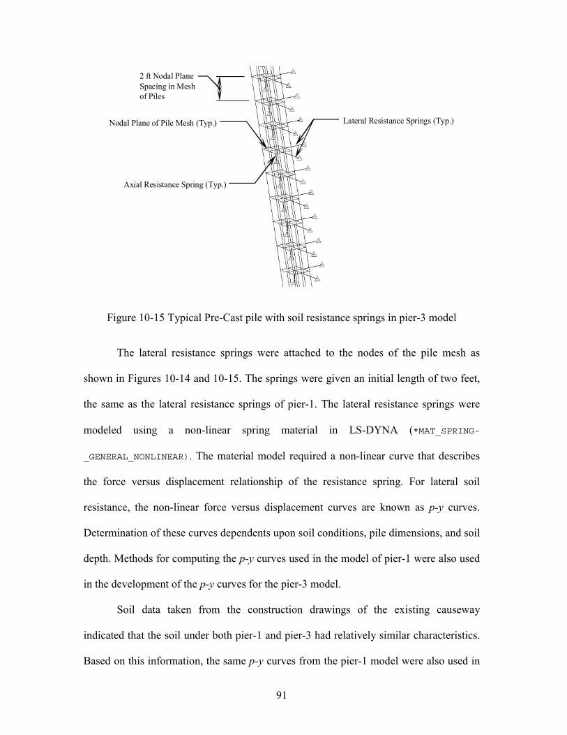
91
Lateral Resistance Springs (Typ.)
Axial Resistance Spring (Typ.)
Nodal Plane of Pile Mesh (Typ.)
2 ft Nodal PlaneSpacing in Meshof Piles
Figure 10-15 Typical Pre-Cast pile with soil resistance springs in pier-3 model
The lateral resistance springs were attached to the nodes of the pile mesh as
shown in Figures 10-14 and 10-15. The springs were given an initial length of two feet,
the same as the lateral resistance springs of pier-1. The lateral resistance springs were
modeled using a non-linear spring material in LS-DYNA (*MAT_SPRING-
_GENERAL_NONLINEAR). The material model required a non-linear curve that describes
the force versus displacement relationship of the resistance spring. For lateral soil
resistance, the non-linear force versus displacement curves are known as p-y curves.
Determination of these curves dependents upon soil conditions, pile dimensions, and soil
depth. Methods for computing the p-y curves used in the model of pier-1 were also used
in the development of the p-y curves for the pier-3 model.
Soil data taken from the construction drawings of the existing causeway
indicated that the soil under both pier-1 and pier-3 had relatively similar characteristics.
Based on this information, the same p-y curves from the pier-1 model were also used in

92
the pier-3 model. Since the spring spacing was shortened from four-feet to two-feet in
the pier-3 model, the MathCad worksheet for interpolating the spring curves was
modified to generate new p-y curves for the added depth increments. In addition to
creating new curves, the values of the p-y curves had to be scaled. The p-y curves are
dependent on the tributary length of pile represented by each spring element. For pier-1,
the springs represent a four foot tributary length of pile, while the springs in pier-3
represent a two foot tributary length of pile. Thus, the p-y curve values from the pier-1
model had to be scaled by fifty percent in order to use them in the model of pier-3.
In addition to the lateral resistance springs, springs were also added to resist the
vertical displacement of the piles. These vertical (axial) springs simulate the skin friction
of the pile face on the surrounding soil. Due to skin friction, an actual pile sheds load
down the length of the pile, distributing the axial load into the soil. Without axial springs
to approximate skin friction, the pile would only have axial resistance at the tip and the
entire load carried by the pile would be transmitted to the tip causing an inaccurate
representation of the pile’s behavior. The axial springs are non-linear like the lateral
resistance springs but however, follow a force versus displacement relationship known
as a T-Z curve. The T-Z curves vary with changing soil conditions much like the p-y
curves for lateral resistance. The axial T-Z curves used in the LS-DYNA models were
computed using formulas based upon soil data. Like the lateral resistance springs, the
same T-Z curves that were used for the model of pier-1 were implemented into the
model of pier-3. Again, modification to the MathCad worksheet for computing the T-Z
curves was required to generate curves for the additional depth increments of pier-3. In
addition, the T-Z curve values required modifications similar to those made for the

93
lateral resistance, p-y springs of pier-1 for use in pier-3. The T-Z curves are dependent
on the surface area of pile approximated by each resistance spring element. Since the
spacing of the axial springs was changed from four feet to two feet from pier-1 to pier-3,
the curve values of the T-Z springs had to be scaled by fifty percent to reflect the change
in total surface area represented by each spring. In general, spring values would have
also been scaled to reflect a change in pile cross-section perimeter. However, in the case
of the HP14x73 piles of pier-1 and the 20 in pre-cast piles of pier-3, the respective
cross-section perimeters differ by two percent. Thus, no modification was required for
the change in pile type. These springs were attached to the central nodes of the pile mesh
as illustrated in Figure 10-14.
The pile springs were constrained in the same manner as in the pier-1 model. All
the free nodes of the resistance springs were fixed in all directions from translational
motion. This was done to provide continuity in results between the models of pier-1 and
pier-3.
94
CHAPTER 11 DETERMINATION OF IMPACT CONDITIONS USING
FINITE ELEMENT SIMULATION
11.1 Introduction
A significant component of the feasibility study involved determining
preliminary values for full-scale barge impact test parameters such as impact velocity
and barge cargo weight. Finite element impact simulation was the primary tool used in
establishing these test parameters. This chapter describes the simulation techniques
employed, impact load histories predicted under varied conditions, and a preliminary set
of proposed test conditions for the full-scale experiments.
In addition, finite element simulation results are compared to barge impact forces
calculated based on the AASHTO Guide Specification and Commentary for Vessel
Collision Design of Bridges (AASHTO 1991). Impact load histories and barge bow
crush depths from the finite element simulations are compared to values calculated using
the AASHTO Guide Specification equations. The equivalent static impact loads
predicted by AASHTO are directly related to the amount of deformation and energy
dissipation that occurs as the headlog of the barge crushes. In this chapter, loads
predicted by the AASHTO method, full dynamic analysis, and static crush simulations
are compared.
In addition to the LS-DYNA impact finite element models, FB-PIER models of
both pier-1 and pier-3 were constructed. FB-PIER has the ability to accurately assess the
ratio of loading demand to total pier capacity for a specified loading condition. Using
these capabilities, safety checks were made to ensure that the impact velocities selected
for the full scale tests do not cause collapse of the piers. The loads specified in the

95
FB-PIER analyses were based on the impact force results generated from the LS-DYNA
dynamic impact simulations (discussed in greater detail later in this chapter).
11.2 Simulation of barge impacts using merged barge and pier finite element models
For the dynamic impact simulations, the LS-DYNA models of pier-1 and pier-3
were merged together with the jumbo hopper barge model. Once combined, two
modifications to the models were required in preparation for the impact simulations. A
contact interface definition had to be specified that permits forces acting between
contacting bodies to be computed and recorded during the simulation. Also, the position
of the barge (in relation to the pier) needed to be established so as to represent a half
loaded draft condition. These modifications are described in the following sections.
11.2.1 Contact definition for determining and recording impact force history
In order to record the time history of the barge impact forces against the bridge
piers, a contact algorithm was established that isolates the interaction of the barge bow
and pier column. Specifically, the LS-DYNA contact algorithm *CONTACT_NODES_TO-
_SURFACE was used for this purpose. The contact interface is defined with the nodes of
the head log mesh as the slave nodes and the element surfaces of the pier column as the
master surface. For reasons of computational efficiency, this contact interface was only
defined for nodes and elements in the region where contact could potentially occur.
Contact interface forces were then recorded at closely spaced time intervals for purposes
of plotting impact force histories (as are shown later in this chapter).
96
11.2.2 Alignment of barge and pier models
When merging the models of the jumbo hopper barge and the piers, it was
necessary to position the barge and bridge pier models in a manner that represented the
desired draft of the barge. The draft of a barge is approximately proportional to the
weight of cargo being carried. Therefore a change in cargo weight causes a change in the
elevation at which the barge head log makes contact with the pier column. The impact
simulations were conducted for a barge that was loaded to half of its total capacity and
which drafted approximately 4ft-6in. Therefore, the barge needed to be positioned such
that after the initialization of gravity forces, the barge bottom was located 4ft-6in below
the zero elevation mark (the waterline) in the finite element model (see Figure 11-1).
Buoyancy SpringsTranslating Base forBuoyancy Springs
Initial and Settled Position of Barge
Waterline
Impact Test Pier
Draft
Contact Zone
Figure 11-1 Desired Alignment of barge model with respect to pier (Pier-1 model)
Because of the method chosen for initialization of gravitational forces for the
barge model, correct positioning of the barge was straightforward (see Section 9.6). By
applying pre-compression to the buoyancy springs to offset the gravitational forces, the
barge model does not change position during the gravity initialization stage of the
97
analysis. This allows the barge draft to be correctly set as shown in Figure 11-1 at the
start of the impact simulation.
11.3 Results for pier-1 impact simulations
Four impact simulations were conducted for head-on impacts of pier-1 (indicated
pier “1-S” for “1-south” in the figures) using a half loaded hopper barge. Impact
velocities simulated included 1 knot, 2 knots, 4 knots, and 6 knots. In the following
figures, time histories of barge-to-pier impact forces are illustrated for the various
impact velocities studied. In addition, plots of impact force versus barge head log crush
depth (barge deformation) are also given. The loads and deformations shown in these
figures are compared to AASHTO predicted values later in this chapter.
Figure 11-2 Impact force vs. time for upper velocity impacts on pier-1

98
Figure 11-3 Impact force vs. time for lower velocity impacts on pier-1
Figure 11-4 Impact force vs. barge bow crush depth for upper velocity impacts on pier-1
99
Figure 11-5 Impact force vs. barge bow crush depth for lower velocity impacts on pier-1
11.4 Results for pier-3 impact simulations
Four impact simulations were also conducted for head-on impacts of pier-3
(indicated pier “3-S” in the figures) using a half loaded hopper barge. Impact velocities
simulated included 0.5 knots, 1 knot, 2 knots, and 4 knots. Time histories of barge-to-
pier impact forces and impact force versus barge crush depth plots are shown in the
following figures. The linear material properties used to model the piles in this pier are
sufficiently accurate to represent the inertial and stiffness characteristics of the pier.
However, such a material model is not capable predicting structural failure of the piles.
As a result, no such failures are indicated in any of the plots that follow. However, it will
be shown later in this chapter, through the combined use of LS-DYNA and FB-PIER,
that pier-3 is structurally capable of resisting only low velocity impact conditions.
100
Figure 11-6 Impact force vs. time for upper velocity impacts on pier-3
Figure 11-7 Impact force vs. time for lower velocity impacts on pier-3
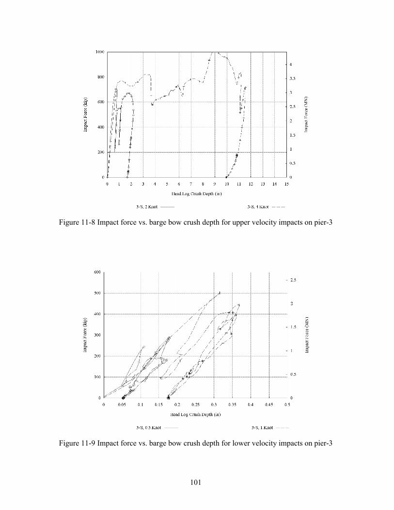
101
Figure 11-8 Impact force vs. barge bow crush depth for upper velocity impacts on pier-3
Figure 11-9 Impact force vs. barge bow crush depth for lower velocity impacts on pier-3
102
11.5 Evaluation of safety using FB-PIER analyses
For safety purposes, both pier-1 and pier-3 were checked for structural stability
with respect to the loads predicted by the dynamic finite element simulations. FB-PIER
models of both piers were obtained from FDOT and modified by the authors to
accommodate the needs of this study. A more detailed soil model, matching the one used
to derive the soil springs used for the LS-DYNA finite element models (see Chapter 10),
was incorporated into both pier models. Additionally, vertical load simulating the weight
of the bridge superstructure was removed from the models to achieve an isolated pier
condition.
Lateral loads applied to the FB-PIER models were obtained from the results of
the LS-DYNA dynamic impact simulations. For each impact condition, the peak
dynamic impact load was determined from the load history and applied to the FB-PIER
pier model as a static lateral load. Applied load magnitudes are shown in Table 11-1.
Ratios of demand to structural capacity computed using FB-PIER are given in
Table 11-2 (where a ratio of 100% percent indicates incipient pier failure). The table
indicates acceptable levels of safety for all of the impact velocities considered for pier-1.
Thus, full scale testing can be performed on pier-1 at any velocity up to 6 knots and
perhaps higher if so desired (additional checks would need to be performed).
Pier-3, in contrast, is not an impact-resistant pier. Based on FB-PIER results, it
appears that impact velocities not exceeding 0.5 knots will be necessary during the full
scale testing if pier failure is to be completely prevented. However, the approach of
applying peak dynamic loads as equivalent static loads to the FB-PIER models is quite
conservative and the actual allowable impact velocity might be higher than 0.5 knots.
The peak dynamic impact loads used are not truly static but rather are transient, short

103
duration load events. Future analysis activities will combine the use of the dynamic
version of FB-PIER (Brown et al. 2001, Fernandez 1999) with the complete dynamic
load histories predicted by LS-DYNA so that more realistic, less overly-conservative
estimations of demand to capacity can be determined. In addition, the impact load
predicted by AASHTO for a velocity of 0.5 knots is considerably less than that predicted
by the LS-DYNA impact simulation (discussed in the next section). Impact velocities in
the range of 0.5 knots to 1 knot are almost certainly feasible for pier-3, but additional
checks will need to be performed before complete confidence in this fact can be
obtained.
Table 11-1 Static loads applied to FB-PIER models
Impact velocity Load applied to pier-1
Load applied to pier-3
½ knot N/A 290 kips (1290 kN) 1 knot 725 kips (3225 kN) 500 kips (2224 kN) 2 knot 875 kips (3892 kN) 700 kips (3114 kN) 4 knot 1000 kips (4448 kN) 810 kips (3603 kN) 6 knot 1200 kips (5338 kN) N/A
Table 11-2 Demand to capacity ratios computed using FB-PIER
Impact velocity Demand to capacity ratio for pier-1
Demand to capacity ratio for pier-3
½ knot N/A 115 % 1 knot 40 % 270 % 2 knot 47 % 400 % 4 knot 53 % 495 % 6 knot 69 % N/A
11.6 Comparison of AASHTO loads, dynamic impact loads, and static crush loads
In this section, impact forces predicted by the AASHTO Guide Specification and
Commentary for Vessel Collision with Bridges are computed so that they can be
104
compared to the results obtained from the preliminary finite element impact simulations
discussed earlier in this chapter. Ultimately, the goal of this research is to compare
impact forces measured during full scale experimental tests to those predicted by
AASHTO. However, a comparison between simulation predicted loads and AASHTO
loads is a useful step in that direction.
To make such a comparison possible, AASHTO barge impact load calculations
were performed for both pier-1 and pier-3. It was only necessary to perform the vessel
collision force calculations, rather than carry out a full probabilistic analysis, because the
proposed impact testing program is concerned primarily with characterizing the isolated,
unfactored impact loads associated with a barge impact event.
A typical jumbo hopper barge traveling at a maximum channel velocity of six
knots was selected as the AASHTO design vessel. In an actual pier design, the barge
impact load would have been calculated using a barge weight corresponding to a fully
loaded condition. In this analysis however, the barge weight was adjusted to correspond
to a half loaded condition. Use of a half loaded barge offers more flexibility in the types
of experimental impact tests that can be conducted, without requiring the addition or
subtraction of barge cargo during testing. Preliminary impact simulations indicated that
pier-3 is not strong enough to sustain an impact from a fully loaded barge. However, it is
able to withstand a low velocity impact from a half loaded barge. As will be
demonstrated shortly, such low velocity impacts warrant experimental investigation and
further consideration.
Results obtained using the AASHTO provisions for both pier-1 and pier-3 are
presented in Table 11-3 (complete calculations are presented in the Appendix). Two sets

105
of AASHTO impact force calculations were performed for pier-3. In the first case, the
impact velocity used was that stipulated by AASHTO based on the location of pier-3
relative to the navigation channel (see Appendix). For this case, the impact velocity was
4.1 knots. In the second case, rather than using the impact velocity stipulated by
AASHTO, a velocity of 0.5 knots was imposed on the analysis and used in all
subsequent calculations (also in Appendix).
Table 11-3 Loads and deformations predicted by AASHTO for a half loaded barge
Impact parameter Pier-1 Pier-3
Impact velocity 6.0 knots 4.1 knots 0.5 knots
Impact force (equivalent static)
1671 kips (7432 kN)
1512 kips (6725 kN)
96 kips (427 kN)
Barge crush depth 35.2 in (894 mm)
17.8 in (452 mm)
0.28 in (7 mm)
Table 11-4 Loads and deformations predicted by dynamic impact simulation for a half loaded barge
Impact parameter Pier-1 Pier-3
Impact velocity 6.0 knots 4.1 knots 0.5 knots
Impact force (peak dynamic)
1200 kips (5338 kN)
1040 kips (4626 kN)
280 kips (1245 kN)
Barge crush depth (max. sustained)
35.0 in (889 mm)
11.5 in (292 mm)
0.18 in (4.6 mm)
Data extracted from the dynamic impact simulation results (Figures 11-2 through
11-9) is summarized in Table 11-4. By comparing this data to that of Table 11-3, the
AASHTO equivalent static load method can be compared to full dynamic impact
106
simulation. For the 6 knot impact on pier-1, the 35 inch crush deformation predicted by
AASHTO compares very well with that of the dynamic impact simulation. However, the
equivalent static load of 1671 kips predicted by AASHTO substantially exceeds even the
peak dynamic load of 1200 kips predicted by the impact simulation. In addition,
although the maximum crush deformations agree well, it is important to note that the
peak impact force in the dynamic simulation occurs not when the barge deformation is at
a maximum, but rather at approximately 10 inches of crush (see Figure 11-4). Thus,
correlating impact load to maximum crush depth may lead to inaccurate force
predictions in some cases. Further investigation in this area, via simulation and physical
testing, is warranted.
For the pier-3 impact conditions, barge deformations predicted by AASHTO
were substantially larger than those the predicted by dynamic simulation for both impact
velocities considered. One possible explanation for this difference is that pier-3 is not an
impact resistant pier and is substantially more flexible than pier-1. Whereas the
AASHTO method and impact simulation predicted similar deformations for the stiffer
pier-1, it appears that the lack allowance for pier flexibility in the AASHTO method
causes significantly different predictions of deformations to occur for smaller piers.
In regard to impact forces, the comparison is more complex. For an impact
velocity of 4.1 knots, the AASHTO method predicted a load larger than that predicted
by impact simulation. However, for the low speed 0.5 knot impact, the load predicted by
AASHTO was smaller than that predicted by impact simulation. The difference is
possibly related to the flexibility of the pier and to the dynamic interaction that occurs
between the barge and the pier during impact. Examining the pier-3 results for a 0.5 knot
107
impact in Figure 11-7, load oscillation is clearly evident as the barge and the pier
dynamically interact during the impact. Loads of approximately 250-300 kips are
reached repeatedly during contact between the barge and the pier. Similar behavior can
be observed in the low velocity impacts simulated for pier-1; in Figure 11-3, multiple
cycles of load are observed as the barge and the pier interact dynamically.
To explore the issue of dynamic response versus static response in more detail,
two sets of “static crush simulations” were conducted using LS-DYNA. In each case, the
base of the barge model was fixed in space while an isolated rigid pier column (without
substructure) was pushed against the barge headlog. In one simulation, the shape of the
rigid pier column matched that of the columns in pier-1 while in the second, the shape
matched that of the columns in pier-3. In both cases, the flexibility of the pier structure
and soil were not part of the simulation. Instead, the rigid pier column was pushed
against the barge at a prescribed rate 10 inches/second. As a result, the barge headlog
experienced an essentially static crush rate (deformation rate) of 10 inches/second. (A
second set of simulations were conducted at 5 inches/second to confirm that
10 inches/second was slow enough to remove all dynamic effects. Results from both
crush rates were virtually identical).
Results from the crush tests provide a way of measuring the relationship between
barge deformation and static contact load with all dynamic effects removed. By
comparing static crush simulation results to the dynamic impact simulation results, the
contribution of dynamic effects during an impact event can be identified. In
Figure 11-10, results from a static crush simulation, a dynamic impact simulation, and
AASHTO calculations are compared for pier-1. In each case, the contact load on the pier

108
is plotted as a function of barge headlog deformation (i.e. crush depth). Comparing the
static and dynamic simulation results, one observes an initial peak the dynamic
simulation that is not present in the static case. Also, at approximately 10 inches of crush
depth, the dynamic simulation predicts a drop in the contact load as the barge is
decelerated. Comparing the AASHTO provisions to the simulation results, two main
points stand out. For small levels of headlog deformation (less than 2 inches), the
AASHTO provisions predict impact loads that are smaller than those predicted using
either simulation. In contrast, for larger levels of deformation, AASHTO predicts loads
that are substantially larger than those predicted by simulation.
Figure 11-10 Comparison of loads predicted by AASHTO method, static simulation, and dynamic impact simulation for pier-1
In Figure 11-11, a similar comparison is provided for pier-3. In this case, the
dynamic loads are moderately smaller than those predicted by a static crush simulation.
Comparing the AASHTO results to the simulation results, we observe the same trends as
109
those evident for pier-1. For small levels of headlog deformation, AASHTO predicts
impact loads that are smaller than those predicted using simulation but for larger levels
of deformation, AASHTO predicts loads substantially larger than those predicted by
simulation.
These trends partially explain the observations made earlier regarding the data in
Tables 11-3 and 11-4. For the 0.5 knot impact on pier-3, very little deformation results
and, as is consistent with Figures 11-10 and 11-11, the AASHTO provisions predict
loads that are smaller than those predicted by simulation. In contrast, for larger levels of
barge deformation, as occurred during the higher velocity impacts cited in Tables 11-3
and 11-4, AASHTO predicts loads that are larger than those predicted by simulation. If
the experimental barge impact test program produces results that are consistent with
these simulation results, then modifications to the AASHTO barge impact provisions
may be warranted.
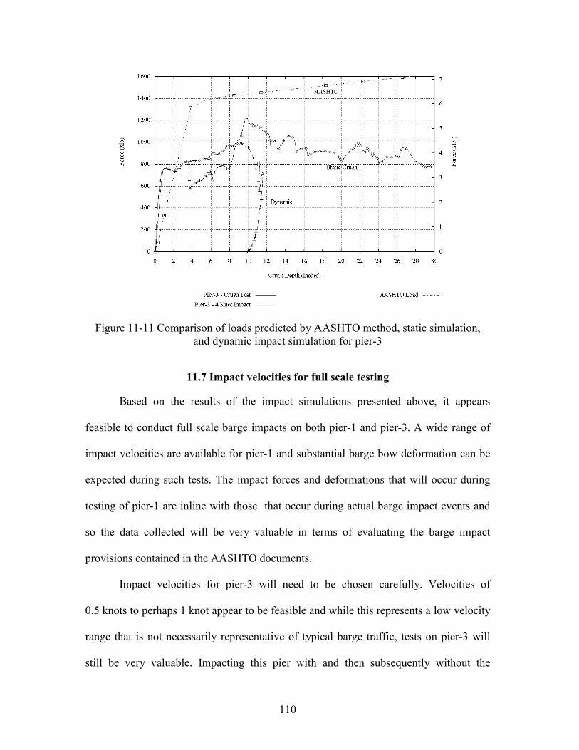
110
Figure 11-11 Comparison of loads predicted by AASHTO method, static simulation, and dynamic impact simulation for pier-3
11.7 Impact velocities for full scale testing
Based on the results of the impact simulations presented above, it appears
feasible to conduct full scale barge impacts on both pier-1 and pier-3. A wide range of
impact velocities are available for pier-1 and substantial barge bow deformation can be
expected during such tests. The impact forces and deformations that will occur during
testing of pier-1 are inline with those that occur during actual barge impact events and
so the data collected will be very valuable in terms of evaluating the barge impact
provisions contained in the AASHTO documents.
Impact velocities for pier-3 will need to be chosen carefully. Velocities of
0.5 knots to perhaps 1 knot appear to be feasible and while this represents a low velocity
range that is not necessarily representative of typical barge traffic, tests on pier-3 will
still be very valuable. Impacting this pier with and then subsequently without the

111
superstructure in place will enable determination of load transfer through the
superstructure. Since pier-3 is non-impact resistant, substantial deformation in the piles
and soil can be expected. Repeated impacts on this pier will cause little or no barge
damage, and can be used to study soil stiffness under extreme loading conditions. Soil
pore pressures can also be measured to determine whether rate effects are important in
barge impact events. Thus, even though low velocity impact will need to be used for
pier-3, a wealth of information can still be obtained from such testing.
Finally, it is worth noting that it would be appropriate to also consider impact
conditions for pier-2 in subsequent phases of this project. Pier-2 is similar to pier-1 but
is not as stiff or as strong. Thus, impact tests on pier-2 as an isolated system would allow
comparisons to be made with the results from tests on the more massive pier-1 and the
more flexible pier-3.

112
CHAPTER 12 CONCLUSIONS
12.1 Assessment of feasibility for full-scale barge impact test program
Based on all areas investigated in this Phase I study, the authors believe that the
full-scale barge impact testing of the St. George Island causeway bridge is feasible.
Listed below are brief summaries of the major items considered in this study along with
cross-references to sections in this report where detailed discussions can be located.
• Environmental permits for proposed testing program
The Apalachicola bay area has stringent restrictions on marine activity due to
environmental protection, however, the proposed impact testing program is still
deemed to be feasible. This assessment is based on the previous success of the
design/build team of Boh Brothers and Sverdrup, Inc. in acquiring the permits
necessary to construct the new bridge and demolish the existing bridge. The
environmental feasibility of the impact testing program is discussed in further detail
in Chapter 4.
• Acquisition of a jumbo hopper barge, tug boat, and tug operator
Jumbo hopper barges are routinely in operation on the inland waterways of Florida. In
addition, a large number of qualified personnel are available in the area of the impact
testing site to pilot a tug boat for navigation of such a hopper barge. As a result, it is
deemed feasible for FDOT to acquire a functional jumbo hopper barge, tug boat, and
tug operator prior to the full-scale testing occurs. For further information on the
requirements of the test barge and tug boat refer to Chapter 5.
113
• Geographic concerns for safe navigation of barge
Based upon a depth survey (conducted by the authors) of the bay bottom area around
the existing bridge, it has been determined that it is feasible to safely navigate and
maneuver a jumbo hopper barge into and around the existing St. George Island
causeway bridge. The results of the bathymetric survey and details on the geographic
feasibility of the impact testing program are discussed in Chapter 6.
• Coincident scheduling of barge testing activities and contractor demolition
Discussions with the demolition contractor for the existing St. George Island
causeway bridge indicated full cooperation with regard to integrating the testing
program into the contractor’s demolition schedule. Thus, complications in scheduling
are not expected for the testing program. A specific schedule for the testing program
with respect to the demolition of the causeway is outlined in Chapter 7.
• Feasibility of conducting impact testing with realistic impact loads while ensuring
safety
Based on the results of impact finite element simulations and FB-PIER analyses, it is
deemed feasible to conduct impact tests on the impact resistant pier-1 at various
velocities while maintaining adequate safety through the testing process. In addition,
it appears that low velocity impact tests are feasible with regard to the non-impact
resistant, pier-3. However, further attention will need to be given to establishing safe
impact conditions for this pier. In addition, it may be appropriate to consider
including impact on pier-2 in the proposed test program. The results of the finite
element model simulations and the FB-PIER analyses are discussed in detail in
Chapter 11.
114
REFERENCES AASHTO, Guide Specification and Commentary for Vessel Collision Design of Highway
Bridges, American Association of State Highway and Transportation Officials,
Washington, D.C., 1991.
AASHTO, LRFD Bridge Design Specifications and Commentary, American Association
of State Highway and Transportation Officials, Washington, D.C., 1994.
Hoit, M. I., McVay, M., Hays, C., and Andrade, W., Nonlinear Pile Foundation Analysis
Using Florida-Pier, ASCE Journal of Bridge Engineering, Volume 1 Number 4, pp
135-142, 1996.
Knott, M., Prucz, Z., Vessel Collision Design of Bridges: Bridge Engineering Handbook,
CRC Press LLC, 2000.
Larsen, O. D., Ship Collision with Bridges: The Interaction between Vessel Traffic and
Bridge Structures, IABSE Structural Engineering Document 4, IASBE-AIPC-
IVBH, Zurich, Switzerland, 1993.
Livermore Software Technology Corporation (LSTC), “LS-DYNA Keyword Manual :
Version 950”, Livermore, C.A., 1999.
Livermore Software Technology Corporation (LSTC), “LS-DYNA Theoretical Manual”
Livermore, C.A., 1998.
Minorsky, V. U., An Analysis of Ship Collisions with Reference to protection of Nuclear
Power Plants, Journal of Ship Research, Volume 3, number 2, pp 1-4, 1959.
115
Patev, R. C., Full-Scale Barge Impact Experiments, Transportation Research Board
Circular 491, Transportation Research Board, Washington, D.C., 1999.
Wekezer, J. W., Yazdani, N., and Wilson, C. M. D., Static Finite Element Analysis of
Bridge Fenders for Barge Impact, ASCE Journal of Performance of Constructed
Facilities, pp 90-95, August 2001.
Whirley, R. G., Engelmann, B. E., Automatic Contact Algorithm in DYNA3D for
Crashworthiness and Impact Problems, Nuclear Engineering and Design, Volume
150, pp 225-233, 1994.
Whitney, M. W., Harik, I. E., Griffin, J. J., and Allen, D. L., Barge Collision Design of
Highway Bridges, ASCE Journal of Bridge Engineering, Volume 1 Number 2, pp
47-58, 1996.
Yazdani, N., Wekezer, J. W., Wilson, C. M. D., and Wuttrich, R., Investigation of Fender
Systems for Vessel Impact, Final Report prepared for the Florida Department of
Transportation, WPI 510846, 2000.

116
APPENDIX
BARGE IMPACT FORCE CALCULATIONS
(Based on the AASHTO “Guide specification and commentary for vessel collision design of highway bridges”)

117
Empty Disp. (TON) - WB_E 200:=
Cargo Disp. (TON) - WB_C 850:=
Number of Barges in Tow - NB 1:=
Channel Parameters...
Channel Width (FT) - BC 250:=
Distance from Center line of Channel to Pier (FT) - LP 125:= Distance to main channel pier (Pier 1-N or 1-S)Water Depth at Pier Location (FT) - DC 7:=
________________________________________________________________________________________
Compute total length of vessel...
LOA LB NB⋅ LT+:= LOA 235= (FT)
Create function to compute code based barge velocity (Figure 3.7-1)...
x 0 4 LOA⋅..:=V x( ) xC BC 2÷←
xL 3 LOA⋅←
V VT← x xC≤if
V VTVT VMIN−
xL xC−x xC−( )⋅−
← xC x< xL≤if
V VMIN← x xL>if
V
:=
0 500 10000
5
10
15
V(x) - Impact Speed Vs. Disp to Centerline
AASHTO - Barge impact force design calculations - Pier-1Saint George Island Causeway, Apalachicola, Florida
This sheet goes through the necessary calculations needed to compute the impact forces for a barge impact event. The calculations are straight from the AASHTO Guide Specification and Commentary for Vessel Collision Design of Highway Bridges.
________________________________________________________________________________________
Variable input:
Barge Parameters... Tow / Push Boat Parameters...
Length of Barge (FT) - LB 195:= Length of Boat (FT) - LT 40:=
Width of Barge (FT) - BM 35:= Empty Disp. (TON) - WT_E 120:=
Head Log Depth (FT) - HL 2:= Typ Boat Vel. (FT/S) - VT 10.127:=
Empty Draft (FT) - DE 1.75:= Min Boat Vel. (FT/S) - VMIN 3.376:=

118
Compute vessel coliision energy "KE" (Equation 3.8-1)...
KECH Wtonne⋅ V LP( )( )2⋅
29.2:= KE 3727.2= (kip-ft)
Compute the barge bow damage depth aB (Equation 3.13-1)...
RB BM 35÷:= ratio of barge width to 35 - parameter needed in damage equation
aB 1 KE
5672+
0.51−
10.2RB
⋅:= aB 2.93= (FT)
Compute the Barge collision force on pier PB (Equation 3.12-1)...
PB 4112aB⋅ RB⋅( ) aB 0.34<if
1349 110 aB⋅+( ) RB⋅ aB 0.34≥if
:= PB_dis PB HL÷:=
PB 1671.3= (KIPS) Total force imparted on pier by barge.
PB_dis 836= (KIPS/FT) Distributed load on pier. (placed along headlog depth.
AASHTO - Barge impact force design calculations - Pier-1Saint George Island Causeway, Apalachicola, Florida________________________________________________________________________________________
Create a function to determine the loaded draft of the barge...
Function uses a simple ratio of cargo weight and bargeself weight to determine the loaded draft.
DLWB_C WB_E+( ) DE⋅
WB_EDE+:= DL 10.938= (FT)
Create function to determine the CH - hydrodynamic mass coefficient...
Values for CH are found in the AASHTO Guide Specification
CH 1.0:=
NOTE: CH is a mass coefficient multiplier to compensate for the mass of water traveling with
the barge. This value is typically set to 1.05 or 1.25 when doing an AASHTO Analysis. However, for the purpose of this analysis the value was set to 1.0 for comparison to the LS-DYNA dynamic simulations which have no compensation for this additional hydrodynamic mass.
Compute total vessel displacement...
W WB_E WB_C+( ) NB⋅ WT_E+:= W 1170= (TON)
Wtonne W 1.1025÷:= Wtonne 1061= (TONNE)
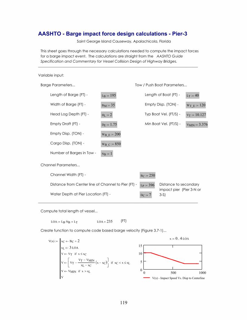
119
Empty Disp. (TON) - WB_E 200:=
Cargo Disp. (TON) - WB_C 850:=
Number of Barges in Tow - NB 1:=
Channel Parameters...
Channel Width (FT) - BC 250:=
Distance from Center line of Channel to Pier (FT) - LP 396:= Distance to secondary impact pier (Pier 3-N or 3-S)Water Depth at Pier Location (FT) - DC 7:=
________________________________________________________________________________________
Compute total length of vessel...
LOA LB NB⋅ LT+:= LOA 235= (FT)
Create function to compute code based barge velocity (Figure 3.7-1)...
x 0 4 LOA⋅..:=V x( ) xC BC 2÷←
xL 3 LOA⋅←
V VT← x xC≤if
V VTVT VMIN−
xL xC−x xC−( )⋅−
← xC x< xL≤if
V VMIN← x xL>if
V
:=
0 500 10000
5
10
15
V(x) - Impact Speed Vs. Disp to Centerline
AASHTO - Barge impact force design calculations - Pier-3Saint George Island Causeway, Apalachicola, Florida
This sheet goes through the necessary calculations needed to compute the impact forces for a barge impact event. The calculations are straight from the AASHTO Guide Specification and Commentary for Vessel Collision Design of Highway Bridges.
________________________________________________________________________________________
Variable input:
Barge Parameters... Tow / Push Boat Parameters...
Length of Barge (FT) - LB 195:= Length of Boat (FT) - LT 40:=
Width of Barge (FT) - BM 35:= Empty Disp. (TON) - WT_E 120:=
Head Log Depth (FT) - HL 2:= Typ Boat Vel. (FT/S) - VT 10.127:=
Empty Draft (FT) - DE 1.75:= Min Boat Vel. (FT/S) - VMIN 3.376:=
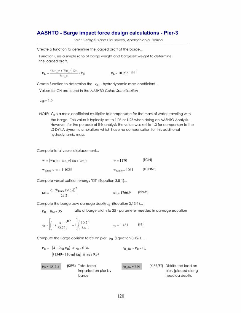
120
Compute vessel coliision energy "KE" (Equation 3.8-1)...
KECH Wtonne⋅ V LP( )( )2⋅
29.2:= KE 1766.9= (kip-ft)
Compute the barge bow damage depth aB (Equation 3.13-1)...
RB BM 35÷:= ratio of barge width to 35 - parameter needed in damage equation
aB 1 KE
5672+
0.51−
10.2RB
⋅:= aB 1.481= (FT)
Compute the Barge collision force on pier PB (Equation 3.12-1)...
PB 4112aB⋅ RB⋅( ) aB 0.34<if
1349 110 aB⋅+( ) RB⋅ aB 0.34≥if
:= PB_dis PB HL÷:=
PB 1511.9= (KIPS) Total force imparted on pier by barge.
PB_dis 756= (KIPS/FT) Distributed load on pier. (placed along headlog depth.
AASHTO - Barge impact force design calculations - Pier-3Saint George Island Causeway, Apalachicola, Florida________________________________________________________________________________________
Create a function to determine the loaded draft of the barge...
Function uses a simple ratio of cargo weight and bargeself weight to determine the loaded draft.
DLWB_C WB_E+( ) DE⋅
WB_EDE+:= DL 10.938= (FT)
Create function to determine the CH - hydrodynamic mass coefficient...
Values for CH are found in the AASHTO Guide Specification
CH 1.0:=
NOTE: CH is a mass coefficient multiplier to compensate for the mass of water traveling with
the barge. This value is typically set to 1.05 or 1.25 when doing an AASHTO Analysis. However, for the purpose of this analysis the value was set to 1.0 for comparison to the LS-DYNA dynamic simulations which have no compensation for this additional hydrodynamic mass.
Compute total vessel displacement...
W WB_E WB_C+( ) NB⋅ WT_E+:= W 1170= (TON)
Wtonne W 1.1025÷:= Wtonne 1061= (TONNE)
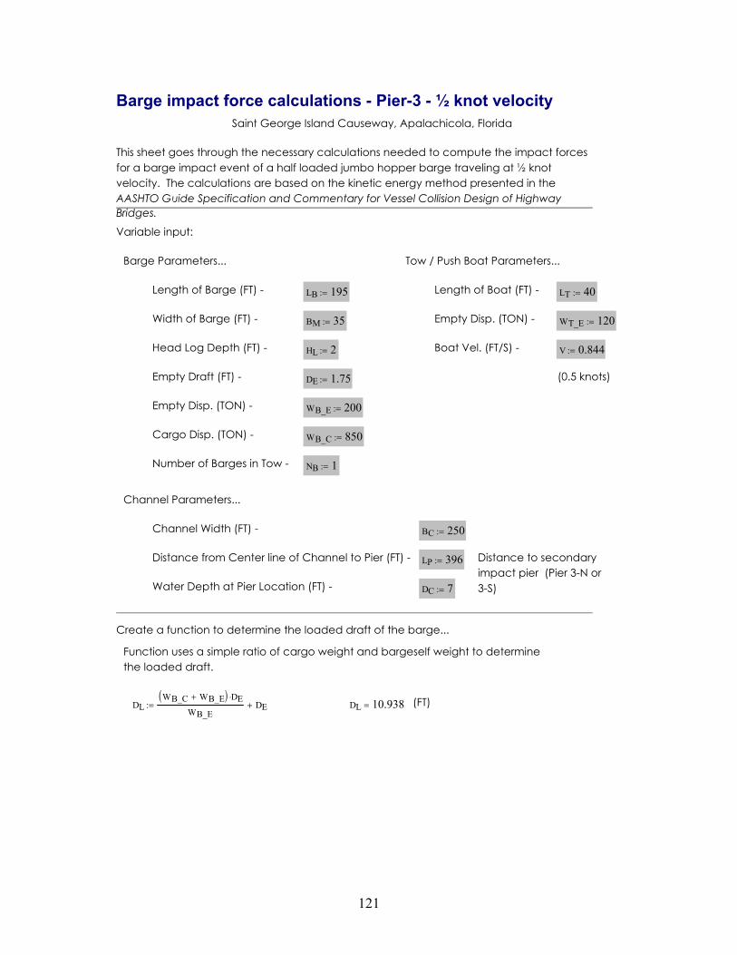
121
(0.5 knots)
Empty Disp. (TON) - WB_E 200:=
Cargo Disp. (TON) - WB_C 850:=
Number of Barges in Tow - NB 1:=
Channel Parameters...
Channel Width (FT) - BC 250:=
Distance from Center line of Channel to Pier (FT) - LP 396:= Distance to secondary impact pier (Pier 3-N or 3-S)Water Depth at Pier Location (FT) - DC 7:=
________________________________________________________________________________________
Create a function to determine the loaded draft of the barge...
Function uses a simple ratio of cargo weight and bargeself weight to determine the loaded draft.
DLWB_C WB_E+( ) DE⋅
WB_EDE+:= DL 10.938= (FT)
Barge impact force calculations - Pier-3 - ½ knot velocitySaint George Island Causeway, Apalachicola, Florida
________________________________________________________________________________________
Variable input:
Barge Parameters... Tow / Push Boat Parameters...
Length of Barge (FT) - LB 195:= Length of Boat (FT) - LT 40:=
Width of Barge (FT) - BM 35:= Empty Disp. (TON) - WT_E 120:=
Head Log Depth (FT) - HL 2:= Boat Vel. (FT/S) - V 0.844:=
Empty Draft (FT) - DE 1.75:=
This sheet goes through the necessary calculations needed to compute the impact forces for a barge impact event of a half loaded jumbo hopper barge traveling at ½ knot velocity. The calculations are based on the kinetic energy method presented in the AASHTO Guide Specification and Commentary for Vessel Collision Design of Highway Bridges.
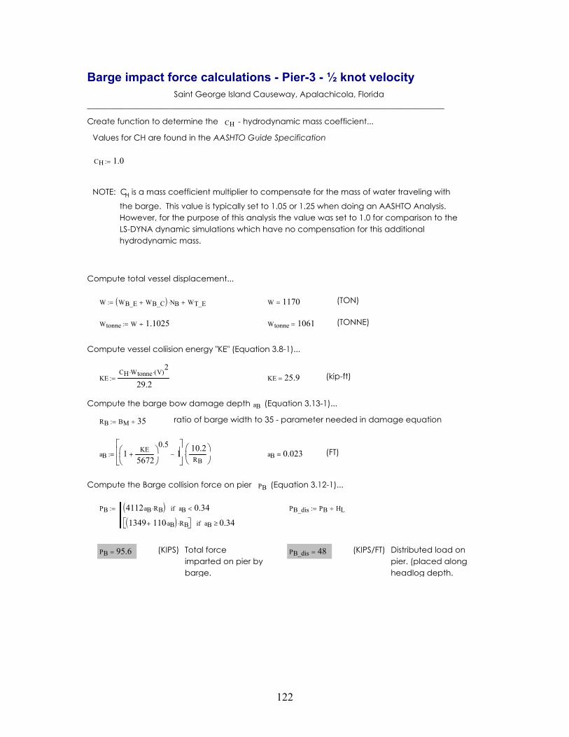
122
Distributed load on pier. (placed along headlog depth.
(KIPS/FT)PB_dis 48=Total force imparted on pier by barge.
(KIPS)PB 95.6=
PB_dis PB HL÷:=PB 4112aB⋅ RB⋅( ) aB 0.34<if
1349 110 aB⋅+( ) RB⋅ aB 0.34≥if
:=
Compute the Barge collision force on pier PB (Equation 3.12-1)...
(FT)aB 0.023=aB 1 KE
5672+
0.51−
10.2RB
⋅:=
ratio of barge width to 35 - parameter needed in damage equationRB BM 35÷:=
Compute the barge bow damage depth aB (Equation 3.13-1)...
(kip-ft)
Barge impact force calculations - Pier-3 - ½ knot velocitySaint George Island Causeway, Apalachicola, Florida
________________________________________________________________________________________
Create function to determine the CH - hydrodynamic mass coefficient...
Values for CH are found in the AASHTO Guide Specification
CH 1.0:=
NOTE: CH is a mass coefficient multiplier to compensate for the mass of water traveling with
the barge. This value is typically set to 1.05 or 1.25 when doing an AASHTO Analysis. However, for the purpose of this analysis the value was set to 1.0 for comparison to the LS-DYNA dynamic simulations which have no compensation for this additional hydrodynamic mass.
Compute total vessel displacement...
W WB_E WB_C+( ) NB⋅ WT_E+:= W 1170= (TON)
Wtonne W 1.1025÷:= Wtonne 1061= (TONNE)
Compute vessel coliision energy "KE" (Equation 3.8-1)...
KECH Wtonne⋅ V( )
2⋅
29.2:= KE 25.9=