Embed Size (px)
Citation preview

ESL-TR-85-52
cv) VOLUME II
CN
IN SITU BIOLOGICAL TREATMENTTEST AT KELLY AIR FORCE BASE,VOLUME !1: FIELD TEST RESULTSAND COST MODEL
R.S. WETZEL, C.M. DURST, D.H. DAVIDSON, D.J. SARNO
SCIENCE APPLICATIONS INTERNATIONAL CORPORATION8400 WEST PARK DRIVEMCLEAN VA 22101
JULY 1987 DTIClftELECTE"ý
FINAL REPORT DEC 1 2 19881
JUNE 1985 -MAY 1987
I I II
APPROVED FOR PUBLIC RELEASE: DISTRIBUTION UNLIMITED
ENGINEERING & SERVICES LABORATORYAIR FORCE ENGINEERING & SERVICES CENTERTYNDALL AIR FORCE BASE, FLORIDA 32403
88 1 12

NOTICE
PLEASE DO NOT REQUEST COPIES OF THIS REPORT FROM
HQ AFESC/RD (ENGINEERING AND SERVICES LABORATORY),
ADDITIONAL COPIES MAY BE PURCHASED FROM:
NATIONAL TECHNICAL INFORMATION SERVICE
5285 PORT ROYAL ROAD
SPRINGFIELD, VIRGINIA 22161
FEDERAL GOVERNMENT AGENCIES AND THEIR CONTRACTORS
REGISTERED WITH DEFENSE TECHNICAL INFORMATION CENTER
SHOULD DIRECT REQUESTS FOR COPIES OF THIS REPORT TO:
DEFENSE TECHNICAL INFORMAIION CENTER
CAMERON STATION
ALEXANDRIA, VIRGINIA 22314
L UNCLA5S1FIED ASECURITY CLASSIFICATION OF THIS PAGE 1 ?o 2
I I lll II IIForm Approved
REPORT DOCUMENTATION PAGE FMBNo. A704-01ov
la REPORT SECURITY CLASSIFICATION lb RESTRICTIVE MARKINGS
IUNCLASSIFIED I2a. SECURITY CLASSIFICATION AUTHORITY 3 DISTRIBUTION/AVAILABILITY OF REPORT
Approved for public release, distribution2b DECLASSIFICATION I DOWNGRADING SCHEDULE unl imi ted.
4. PERFORMING ORGANIZATION REPORT NUMBER(S) S. MONITORING ORGANIZATION REPORT NUMBER(S)
ESL TR-85-52-II
6a. NAME OF PERFORMING ORGANIZATION 6b OFFICE SYMBOL 7a. NAME OF MONITORING ORGANIZATIONScience Applications Inter- (if applicable) Air Force Engineering and Services Centernational Corporation I6c. ADDRESS (City, State, and ZIP Code) 7b. ADDRESS (City, State, and ZIP Code)
8400 Westpark Drive HQ AFESC/RDVWMcLean, Virginia 22102 Tyndall AFB, Florida 32403-6001
Ba. NAME OF FUNDING/SPONSORINGON 8b OFFICE SYMBOL 9 PROCUREMENT iNSTRUMENT IDENTIFICATION NUMBER
ORGANIZATION (if applicable)
(See reverse) j _______ MIPR No. FY8952-85-100235c. ADDRESS (City, State, and ZIP Code) 10 SOURCE OF FUNDING NUMBERS
PROGRAM IPROJECT ITASK IWORK UNITELEMENT NO NO NO ACCESSION NO
64708F 2054 30 5511 TITLE (Include Security Classification)
In Situ Biological Treatment Test at Kelly Air Force Base, Volume II: Field Test Resultsand Cost Model (UNCLASSIFIED)
12 PERSONAL AUTHOR(S)Roger S. Wetzel, Connie M. Durst, Donald H. Davidson, and Douglas J. Sarno
l3a. TYPE OF REPORT 113b TIME COVERED i " 4. DA•E OF REPORT (Year, Month, Day) 115. PAGE COUNTFinal F FROM 850601 To8 7 05 31 i July 1987 170
16. SUPPLEMENTAP.Y NOTATION
Availability of this report is specified on reverse of front cover.
17. COSATI CODES 18. SUBJECT TERMS (Continue on reverse if necessar.y and identify by block number)
FIELD GROUP SUB-GROUP Environmental Engineering (continued on reverse)13 02 Z Ground Water05 13 .Water Treatment
19 ABSTRACT (Continue on reverse if necessary and identify by block number)
"-zNThe objective of this effort was to field test in situ biodegradaticn to treat aquifercontamininants. In situ biodegradation is enhanced 5B- stimulating the indigenous subsurfacemicrobial populatT-n- oythe addition of nutrients and an oxygen source to promote degradationof organic contaminants. In situ treatment affects contaminants sorbed to soil as well asdissolved in groundwater. It is potentially faster, and therefore cheaper, than conventionalpump-and-treat technologies.
The test site, located at Kelly AFB, Texas, was contaminated with a mixture of organicand inorganic chemicals. Tne treatment system consisted of an array of nine pumping wellsand four infiltration wells. These wells circulated groundwater and transported the treatmenchemicals throughout the 2800 square feet treatment area. Oxygen was supplied by means ofa hydrogen peroxide solution. Nutrients were principally ammonium and phosphate salts. Thesystem was operated for 9 months.
Data showed evidence of both aerobic and anaerobic biodegradation. Decreases in tetra-rhlnrn~thvl~nP dnd tgrchlnrn~thIlg~ne canncntrationn in groundwat~er correlate with anaerobic20 DISTRIBUTION / AVAILABILITY OF ABSTRACT ". 21 ABTR SEURITY CLASSIFICATION -
rMUNCLASSIFIED/UNLIMI'rED 0 SAME AS RPT [C DTIC USERS UNA F22a NAME OF RESPONSIBLE INDiVIDUAL 22b T dude Area Code) 22 OFFICE YM-OL
Capt Edward HeyseS( AF(E -6 _RD .VWDD Form 1473, JUN 86 Previous editions are obsolete. SECURITY CLASSIFICATION OF THIS PAGE
i UNCLASSIFIED

8. Jointly sponsored and funded by:
Air Force Engineering and Services Center and U.S. Environmental Protection Agenc,HQ AFESC/RDVW HWERLTyndall AFB, Florida 32403-6001 26 West St Clair
Cincinnati, Ohio 45268
18. DESCRIPTORS: 1rob+0iey rMicrobiological Testing e AquifersWaste Treatment /Hydrogen Peroxide HydrologyPollutants, '/Chlorinated Hydrocarbons HydrocarbonsWater Wells,, Aromatic Hydrocarbons ChemistrySCalcium Phosphates Degradation-Ghosts Cost Models Antimony
Heavy Metals Chemical Precipitation PluggingIron Compounds
IDENTIFIERS: Biological Degradation BioreclamationGroundwater Treatment BiodegradationUndeg-tod--uPolfrttents-- I n S i tu
microcosm tests. Aerobic biodegradation was indicated by acid and cabon dioxide productionand increases in petroleum hydrocarbon concentrations in groundwater.) However, anybiodegradation of these hydrocarbons was too small to be quantified. The main problemsexperienced during testing were caused by reactions between injected chemicals and sub-surface minerals. Calcium phosphate precipitation clogged infiltration wells and reducedthe infiltration capacity of the test area by 90 percent. Metal sediments, primarily ironcompounds, were found in the treatment system plumbing. These metals were probablymobilized by chemical reactions resulting from injecting high con:entrations of hydrogenperoxide and nutrients, and may have been transported as small particles. The costs of thein situ treatment test were closely monitored. The technology was found to be no moreepensiTve than conventional technologies.
The study confirms that indigenous bacteria can be enhanced to degrade organiccontaminants. The problems with in situ treatment are primarily those of delivery ofchemicals and minimizing adverse ifacdons between injection chemicals and subsurfaceminerals.
/ \
- I
ii

EXECUTIVE SUMMARY
The objective of this project was to field-test in situ biological
degradation for removal of organic contaminants from soils and ground-
water. In situ biological degradation involves stimulation of the
indigenous subsurface microbial population by the addition of nutrients
and an oxygen source (hydrogen peroxide) to promote degradation of
organic contaminants present in soils and groundwater.
A site was selected for the test at Kelly AFB, Texas. This site,
designated E-1 in the Phase I Installation Restoration Program (IRP)
Report, was contaminated with a mixture of organic and inorganic compounds.
A groundwater circulation system was installed within a 60-foot diameter
portion of the site. This system consisted of nine pumping wells and
four injection wells; groundwater was pumped to a central tank; nutrients
and hydrogen peroxide were then added to the flow before reintroduction
to the subsurface.
Literature review, site characterization, treatability studies,
design, installation, startup, and approximately 3 months of operation
were conducted as an initial phase and are reported in Volume I. Opera-
tion of the system was continued for an additional 5 months. This Volume
II report documents the data collected during the full field operations
period, analysis of system performance, and general considerations and
cost analysis for applications to future sites. Analytical data and
methodologies are presented in Appendix form in Volume III.
The results of the test at Kelly AFB allowed for a number of conclusions
regarding in situ treatment. The low and variable permeabilities at the
test site resulted in a slower delivery of nutrients and oxygen source-
than anticipated, as well as difficult operating conditions, but did not
prevent degradation from occurring.
This Document ContainsMissing Page/s That AreUnavailable In TheOriginal Document.
PIA&E )_7 ~

Data collected during the test shows evidence of degradation of
contaminants by both aerobic and anaerobic means, Decreases in concentra-
tions of PCE, TCE, and hydrocarbons in the groundwater were observed.
A number of other effects of in situ treatment were also observed as a
result of this test. The precipitation of calcium phosphate began almost
immediately upon the introduction of nutrients and hydrogen peroxide.
This precipitation had a negative impact on the project by reducing the
permeabilities of the soil surrounding the injection wells. A migration
of some metal compounds (particularly iron) from soil was also observed
and may have been caused by movement of fine-grained particles in the
subsurface. Work performed on estimating the cost of in situ treatment
showed that full-scale implementation would be no more expensive than
conventional techniques. The cost of performing in situ treatment for
the entire site at Kelly AFB, where the test was performed, was estimated
to be approximately $100 per ton of soil in the saturated zone. The cost
of removal and redisposal was estimated to be $121 per ton.
A number of recommendations were presented regarding the future of in
situ treatment. Recommendations include suggestions for future testing to
determine the cause of calcium phosphate precipitation, study aerobic vs.
anaerobic treatment, develop optimum treatment systems and monitoring
programs, determine the cause of metals mobilization, and develop optimal
nutrient compositions and sources of oxygen. Specific attention was paid
to the requirements that will be posed by applying in situ treatment at a
full-scale installation.
iv

PREFACE
This report was prepared by Science Applications InternationalCorporation (SAIC), 8400 Westpark Drive, McLean, Virginia 22102, underEG & G Idaho, Inc. Subcontract C84-130562 for the Air Force Engineeringand Services Center, Engineering and Services Laboratory, Tyndall AirForce Base, Florida, and the EPA Office of Research and Development,Hazardous Waste Engineering Research Laboratory, Cincinnati, Ohio.
A number of subcontractors and consultants were used to provide special-ized expertise for in situ biological degradation. These subcontractorsinclude: FMC CorporatTi-onAquifer Remediation Systems; Biosystems, Inc.;Dr. C. H. Ward, Rice University; Memphis State University; EnvironmentalResearch Group, Inc.; Hamilton Drilling and Engineering Testing, Inc.;K. W. Brown and Associates; Mr. Paul Rogoshewski; Shilstone EngineeringTesting Laboratories; and Aqualab, Inc.
This technical report is divided into three volumes. Volume I pre-sents work done between May 1984 and September 1985 and discusses indetail the site characterization, laboratory studies, and treatmentsystem design and installation. Volumes II and III summarize the workperformed between October 1985 and February 1987. Volume II discussesthe system operation and performance, results of the field demonstrationproject, and the cost of in situ biological treatment. Analytical dataand methodologies are preenT-e-d-in Appendix form in Volume III. Ms.Barbara Broomfield was the EG & G Idaho, Inc. Project Officer. CaptainEdward Heyse was the AFESC Project Officer, and Mr. Stephen James wasthe EPA Office of Research and Development Project Officer.
This report discusses field demonstration using proprietary formu-lations of nutrients and hydrogen peroxide. It does not constitute anendorsement of these products by EG & G Idaho, Inc., the Air Force orEPA, nor can it be used for advertising the product.
This report has been reviewed by the Public Affairs Office (PA) andis releasable to NTIS. At NTIS, it will be available to the generalpublic including foreign nationals.
This technical report has been reviewed and is approved for publi-cation.
EDWARD HEYSE, Capt., USAF, BSC LAWRENCE D. HOKANSON, Col, USAFProject Officer Director, Engineering and
Services Laboratory
THOMAS J. WALKER, Lt Col,USAF, BSCChief, Environics Division
v
(The reverse of this page is blank)

TABLE OF CONTENTS
Section Title Page
INTRODUCTION . . . . . . . . . . . . . . . . . . . . . . I
A. OBJECTIVE. . . . . . . . . . . . . . . . . . . . . . 1
B. BACKGROUND . . . . . . . . . . . . . . . . . . . . . 1Co SCOPEo 2
II PRELIMINARY ACTIVITIES . . . . . . . . . . . . . . . . . 4
A. LITERATURE REVIEW. . . . . . . . . . . . . . . . . . 4
B. SITE CHARACTERIZATION. . .. . . . . . . . . . . . . 10
1. Geology. . . . . . . . . . . . . . . . . . 122. Hydrology. . . . . . . . . . . . . . . . . 133. Contaminants . . . . . . . . . . . . . . .. 134. Microbiology . . . . ... . . .......... . . . . . 14
C. TREATABILITY STUDIES ................ 14
1. Biodegradation Study . . . . . . . . . . . . . . 142. Permeability Studies . . . . . . . . . . . . . . 22
D. DESIGN AND INSTALLATION OF TREATMENT SYSTEM. . . . . 25
III TEST PROCEDURES. . . . . . . . . . . . . . . . . . . . . 31
A. DESCRIPTION OF FIELD OPERATING PROCEDURES. . . . . . 31
1. System Operation . . . . . . . . . . . . . . . . 312. Sampling Schedule and Procedures . . . . . . . . 32
B. DESCRIPTION OF ANALYTICAL PROCEDURES . . . . . . . . 35
1. Microbiological Enumeration. . . . . . . . . . . 352. Laboratory Cheminal Analyses . . . . . . . . . . 363. Field Chemical Analyses. . . . . . . . . . . . . 37
C. SITE HEALTH AND SAFETY PLAN...... . . . . . . . 39
D. SITE MITIGATION PLAN . ............... 40
vii

TABLE OF CONTENTS (CONTINUED)
Section Title Page
III E. SYSTEM SHUTDOWN. . . . . . . . . . . . . . . . . . . 40
IV SYSTEM PERFORMANCE ................... 41
A. STARTUP. . . . . . . . . . . . . . . . .*. . . . . . 41
B. SCHEDULE OF CHANGES OF OPERATING PARAMETERS. . . . . 42
C. MAJOR OPERATING PROBLEMS. ...... . .. .... 45
D. WELL PATTERN FLOW EFFECTS. . . . . . . . . . . . . . 47
1. Analysis of Changes in GroundwaterCirculation Rates . . . .. . .. ... . 47
2. Fluid Communication in Well Pattern. ...... 51
E. WELL PATTERN CHEMICAL EFFECTS. . . . . . . . . . . . 58
1. Nutrient (Ammonia and Phosphate)Communication. . . . . . . . . . . . . . . . . . 58
2. Hardness Changes in CirculatedGroundwater . . .......... 66
3. Carbon Dioxide (C02) Production ........ 694. Metals Changes in the Soil . . . . . . . . . . . 775. In Situ Acid Generation. . . . .... . . . . . . 866. TWnIMo ing Groundwater Nitrate (N03) . . . . . . 877. Monitoring Groundwater Sulfate (S04 ) . . . . . . 87
F. WELL PATTERN MICROBIOLOGICAL EFFECTS . . . . . . . . 90
G. WELL PATTERN ORGANIC CONTAMINANT CHANGES . . . . . . 97
H. MECHANICAL AND ELECTRICAL EQUIPMENT. . . . . . . . . 106
I. MITIGATION RESPONSE. . . . . . . . . . . . . . . . . 107
J. SAMPLING AND ANALYSIS. . . . . . . . . . . . . . . . 108
K. HEALTH AND SAFETY . . . . . . . . . . . . . . . . . 110
V PROJECT QA/QC. . . . . . . . . . . . . . . . . . . . . . 112
A. QA/QC PLAN . . . . . . . . . . . . . . . . . . . . . 112
viii

TABLE OF CONTENTS (CONTINUED)
Section Title Page
V B. SAMPLING PROCEDURES ............... 112
C. TESTING PROCEDURES .... ............. 113
D. SYSTEM AND PERFORMANCE AUDITS. . . o . . . . . . . . 113
E. PREVENTIVE MAINTENANCE AND ENGINEERINGQUALITY CONTROL. . . . . . . o . o . . . . . . . . 114
VI IMPLEMENTATION AND COST OF IN SITU TREATMENT . . . . . . 115
A. GENERAL CONSIDERATIONS FOR IMPLEMENTING IN SITUBIODEGRADATION . o . . . . . . . .. . . . . . . . 115
1. Site Characterization. . . . ...... 1152. Soil and Groundwater Treatability Studies. .o. . 1173. Design of the Well and Chemical Systems. . . . . 1194. Construction of the System . o . . o . .. . . . 1235. Startup and Operation . . . . . . . . . .. . 124
B. BREAKDOWN OF COSTS AT KELLY...... . . .. ... 124
1. Initial Field Characterization andLaboratory Studies . . o .. . . o . . . . 125
2. Pumping Characterization (January 1985). . .0. . 1253. System Design . . .o o . . o o . . . . . . . . 1254. System Construction and Startup . . . .o . . . 1265. System Operation, Sampling, and Analysis . . . . 1266. Office and Administrative Costs. . . o . .. . . 127
C. COST ESTIMATION FOR IN SITU BIODEGRADATION . . . . . 127
D. SENSITIVITY ANALYSIS FORCONSTRUCTION AND OPERATING COSTS . . .. . . . .. 135
VII SUMMARY OF OBSERVATIONS . . . o . . . . . . . . .. . . 143
VIII CONCLUSIONS . . . . . o . . . . . o . . . . . . . . . 145
A. DEGRADATION RESULTS . . . . . . o . . . . . . .o. . 145
B. SITE CHARACTERISTICS . ... ... . . . .... 145
ix

TABLE OF CONTENTS (CONCLUDED)
Section Title Page
VIII C. TREATMENT CHEMICALS. . . . . . . . . . . . . . . . . 146
D. COST OF IN SITU TREATMENT ...... ........ 146
E. SAMPLING AND ANALYSIS. ............ ... 147
IX RECOMMENDATIONS # * a . e * . . . e . .. . . . . . . 148
A. REQUIREMENTS FOR FULL SCALE IN SITU TREATMENT. . . . 148
B. GENERIC COST MODEL . ................ 149
C. FUTURE TESTS/RESEARCH NEEDS. . . . . . . . . . . . . 149
1. Alternate Injection/Extraction Systems ..... 1502. Nutrient Selection . . . . . . . . . . . . . . . 1503. Use of Hydrcgen Peroxide . . . . . . . . . . . . 1514. Metals Mobilization . . . . . . . . . . . . . . 1515. Precipitation and Clogging . . . . . . . . . . . 1516. Carbon Dioxide Monitoring. . . . . . . . . . . . 1527. Soil Column Testing ................ 152
REFERENCES . . . . . . . . . . . . . . . . . . . . . . . . . . . 154
x

LIST OF FIGURES
Figure Title Page
1 Area of Site Showing Boreholes, Monitoring Wellsand Demonstration Site . . . . . . . . . . . . . . . . . 11
2 Ratio of Unresolved/Resolved HydrocarbonsVersus Time . . . . . . . . . . . . . . . . . . . . . . . 17
3 Chlorobenzene Concentrations Versus Time . . . . . . . . 18
4 Tetrachloroethene (PCE) Concentrations Versus Time . . . 19
5 Trichloroethene (TCE) Concentrations Versus Time . . . . 20
6 Trans 1,2 Dichloroethene (Trans-1,2-DCE)Concentration Versus Time. . . . . . . . . . . . . . . . 21
7 Permeability and Nutrient Solution Breakthroughfor Soil Sample Number One . . . . . . . . . . . . . . . 23
8 Permeability and Nutrient Solution Breakthrough
for Soil Sample Number Two . . . . . . . . . . . . . . . 24
9 System Well Configuration. . . . . . . . . . . . . . . . 27
10 Cross Section of a Typical Pumping Well. . . . . . . . . 2q
11 Plan View of System Configuration. . . . . . . . . . . . 30
12 System Well Configuration Showing SoilSampling Locations . . . . . . . . . . . . . . . . . . . 34
13 Weekly Average Groundwater Circulation . . . . . . . . . 48
14 Initial Permeability of Production Wells . . . . . . . . 54
15 Chemical Tracer Breakthrough. . . . . . . . . . . . . . 55
16 Comparison of Average Chloride Concentrations. . . . . . 57
17 Ammonia and Phosphate Ratios for Well P5 . . . . . . . . 61
18 Ammonia and Phosphate Ratios for Well P8 . . . . . . . . 62
19 Nutrient Breakthrough. . . . . . . . . . . . . . . . . . 63
xi

LIST OF FIGURES (CONCLUDED)
Figure Title Page
20 Ammonia to Chloride Ratios for Well P9 and Averageof Injection Wells . . . . . . . . . . . . . . . . . . . 64
21 Comparison of Average Hardness Levels in Pumpingand Monitoring Wells . . . . . . . . . . . . . . . . . . 67
22 Hardness Breakthrough. . . . . . . . . . . . . . . . . . 68
23 Average Hardness Levels for Injection Wells. . . . . . . 70
24 Comparison of Average CO2 Levels . . . . . . . . . . . . 72
25 CO2 Concentrations in Wells M1, M2, P2, P5, and P9 . . . 73
26 Carbon Dioxide Breakthrough. . . . . . . . . . . . . . . 76
27 Average of Bacteria Counts for Injection Wells . . . . . 92
28 Average of Bacteria Counts for Pumping Wells . . . . . . 93
29 Bacteria Counts for Soil .. ............. . 94
30 Bacteria Counts for Well M1. . . . . . . . . . . . . . . 95
31 Bacteria Counts for Well M2. . . . . . . . . . . . . . . 96
32 Site Characterization for In Situ Treatment. . . . . . . 116
33 Cost Estimation Worksheets . . . . . . . . . . . . . . . 130
34 Characteristics of Baseline Scenario Used for CostSensitivity Analysis . . . . . . . . . . . . . . . . . . 138
xii

LIST OF TABLES
Table Title Page
1 Representative Concentrations of Contaminants atthe Demonstration Site .*. . . . . . . . . . . .. . .. 15
2 Groundwater Monitoring Schedule. . . . . . . . . .. . 33
3 Summary of System Operating Parameter Changes. . . . . . 43
4 Summary of System Operation Changes. . . . . . . . . . . 49
5 Summary of Relative Well Pattern Chemical Responses... 52
6 Materials Inventory of Chemicals Added toGroundwater. . . . . . . . . . . . . . . . . . . . . . . 59
7 Summary of Comparisons of Soil Metal Changes DuringSystem Operation . . . . . . . . . . . . . . . . . . . . 78
8 Summary of U.S. Bureau of Mines Analysis of KellySoil Samples . . . . . . . . . . . . . . . . . . . . . . 81
9 Selected Trace Metal Concentrations in Water and Soils
Before and on Day 49 of the Laboratory Study . . . . . . 83
10 Summary of pH Variations . . . . . . . . . . . . . . . . 88
11 Average Sulfate Concentrations in Groundwater. . . . . . 89
12 Summary of Ranges and Averages of Bacteria Counts .... 91
13 Concentrations of Total Hydrocarbons and Oil andGrease in Soil . . . . . . . . . . . . . . . . . . . . . 99
14 Total Hydrocarbons in Groundwater, GC Scan (ppm) .... 100
15 Oil and Grease in Groundwater (ppm). . . . . . . . . . . 101
16 Summary of Groundwater TCE, PCE, and Trans-1,2-DCEChanges During Treatment . . . . . . . . . . . . . . . . 102
17 Volatile Priority Pollutant Concentrations in Soil . . . 104
18 Total Concentration of Volatile Priority Pollutantsin Groundwater (ppm) . . . . . . . . . . . . . . . . . . 105
xiii

LIST OF TABLES (CONCLUDED)
Table Titte Page
19 Description of Variables Used on Cost EstimationWorksheets . . . . . . . . . . . . . . . . . . . . . . . 128
20 Summary of Cost Sensitivity Analysis Results . . . . . . 140
xiv

SECTION I
INTRODUCTION
A. OBJECTIVE
The purpose of this project was to test in situ biological degrada-
tion under actual field conditions and to determine its applicability to
cleaning up hazardous waste sites and waste-contaminated soil and ground-
water. The technology was field-tested on a hazardous waste site at
Kelly AFB, San Antonio, Texas. In situ biological degradation can be at
least as effective as other remedial technologies at a lower overall
cost. In situ technology can treat those contaminants sorbed to soil
particles as well as those dissolved in groundwater. In situ treatment
may, therefore, be more effective for sorbtive contaminants than are con-
ventional pump-and-treat technologies which treat only groundwater.
B. BACKGROUND
In situ biological degradation of contaminants in soil and ground-
water involves stimulation of the indigenous subsurface microbial popu-
lation to promote degradation of organic contaminants. The tested pro-
cess uses aerobic degradation pathways requiring that a source of oxygen
be supplied to the subsurface environment to maintain aerobic conditions.
Previous studies have shown that conventional aeration techniques cannot
consistently supply an adequate amount of oxygen for in situ treatment.
Thus, the amount of degradation that occurs is limited. The field test
at Kelly AFB will help evaluate the effectiveness of using hydrogen
peroxide as an oxygen source; hydrogen peroxide can provide as much as 50
times the level of oxygen provided by conventional aeration. Nutrients,
such as nitrogen and phosphorus, are also added to the subsurface to en-
hance the growth of the microbial population.
1

C. SCOPE
The field test was performed within a 60-foot diameter area located
on waste site E-1 in the Installation Restoration Program (IRP) Phase I
study at Kelly AFB Within this area, nine pumping wells and four gravity
injection wells were placed to circulate groundwater. A specially formu-
lated nutrient solution and stabilized hydrogen peroxide were added to the
groundwater flow and transported to the subsurface to enhance the ability
of the indigenous microbes to degrade contaminants.
This project included a feasibility study and a laboratory treat-
ability study to evaluate potentially applicable in situ treatment options
and to optimize their design. A pilot-scale in situ treatment system was
installed, operated, and monitored for 8 months at a waste site at Kelly
Air Force Base.
Volume I of this report included project activities from May 1984
through September 1985 as well as detailed site characterization activities. Thes
activities included the determination of site stratigraphy, soil perme-
ability, and hydraulic conductivity. Enumeration of both soil and ground-
water microbes was conducted to determine if an adequate population was
present for successful biodegradation of the organic contaminants. A
full inorganic and organic contaminant profile of the subsurface soils
and groundwater was derived. Treatability studies were conducted to
determine the effect of treatment to onsite soils. Nutrients and
hydrogen peroxide were added to columns containing soil from the Kelly
AFB site to determine biodegradability of contaminants using soil/ground-
water microcosms. Volume I also discusses design, implementation, start-
up, and 3 months of operation.
Volume II, focuses on the operation of the system, conclusions, and
recommendations for future applications of in situ biological degradation.
Section II gives a brief summary of previous project activities. Section
2
III discusses operational procedures followed, including system operation,
sampling schedule and procedures, analytical procedures, health and safety
procedures, plan for mitigating spills and any uncontrolled releases of
contaminants during the operation of the system, and system shutdown pro-
cedures. Section IV discusses system performance, operational problems and
data relating to hydrogeological, chemical, and microbiological changes
observed during the 8 month demonstration period. Section V includes
project Quality Assurance/Quality Control (QA/QC) procedures followed.
Section VI discusses the planning and cost associated with full-scale
implementation of in situ treatment. Section VII presents a summary of
observations at the Kelly AFB test. Sections VIII and IX present Conclu-
sions and Recommendations, respectively.
Volume III contains appendixes A-E with additional information,
includinq analytical data and methodologies.
3

SECTION II
PRELIMINARY ACTIVITIES
The field test was preceded by a literature review, site character-
ization, and treatability studies. Information gained from these studies
was used to design the treatment system. The results of these studies and
detailed descriptions of system design and installation were presented in
Volume I and are summarized in this section.
A. LITERATURE REVIEW
In situ biodegradation is a technical outgrowth of land-spreading
technology, a process primarily used by petroleum refineries to dispose
of oily sludges from storage and processing facilities. Land-spreading
involves the mixing of biodegradable sludge and fertilizer into the
soil using a tiller or dozer and allowing the indigenous soil micro-
organisms to multiply and degrade the waste material. Exxon's Baytown
refinery has been disposing of oily wastes by land farming since 1953
(Reference 1).
Formal research on the land spreading technique began in the 1970s.
In 1972, a report for the U.S. EPA was prepared by Shell Oil Company,
summarizing 18 months of research on land-spreading of three types of
oily wastes: crude oil tank bottoms, Bunker C fuel oil, and waxy
raffinate wastes (Reference 2). Biodegradation rates were found
to be about 70 barrels per acre of soil per month. The population of
soil microbes was found to increase during the study period to over
108 organisms per grain of soil. Major species of microorganisms in-
cluded members of the genus Pseudomonas, Flavobacterium, Nocardia,
Corynebacterium, and Arthrobacter.
4

Sun Ventures, Inc., a subsidiary of Sun Oil Company, also con-
ducted research on oily waste land farming (Reference 3). Their 18-
month project involved three field sites and six types of oily wastes.
Results indicated a naturally occurring hydrocarbon-utilizing bacterial
population that reached levels of about 10 million organisms per grain
of soil 1 year after the initial application. Removal efficiencies of
oil ranged from 48.5 to 90 percent depending on the type of waste and
location.
In the early 1970s, Sun Ventures developed the in situ biodegrada-
tion precess as a means of treating contaminated subsurface soils and
groundwater. In 1971, Sun Pipe Line Company experienced a gasoline
pipeline break in Ambler, Pennsylvania, which spilled more than 3,000
barrels of high-octane product into the groundwater (Reference 4).
Gasoline recovery by pumping was effective for removing only about 50
percent of the gasoline. Additional pumping to remove residual con-
tamination proved futile. The problem was referred to Sun Ventures,
which proposed in situ biodegradation as a means of removing the re-
maining gasoline contamination.
After conducting a series of treatability studies, Sun Ventures
confirmed that the active bacterial population present in the subsurface
could degrade the gasoline when provided with certain nutrients and
oxygen. The actual cleanup was conducted by adding nitrogen and phos.-
phorus to the groundwater in the form of (NH4 ) 2 SO4 , Na2 HPO 4 ,
and NaH 2 PO4. Oxygen was provided by injecting air into the groundwater
via a series of diffuser wells connected to paint-sprayer type com-
prassors. The flow of groundwater was controlled by a series
of injection and extraction wells. An estimated 744 to 944 barrels of
gasoline were degraded. Ten montns after the addition of nutrients, no
gasoline was found in water from extraction wells (Reference 5).
In 1976, a leak was discovered in an underground gasoline storage
tank in Millville, New Jersey, which contaminated a shallow sandy
5

aquifer and caused gasoline vapor problems in the basements of nearby
houses. Again, physical recovery efforts could only remove a portion
of the spilled product. In situ biodegradation of the contaminated
aquifer was carried out by SunTech, Inc. (Sun Ventures, Inc.) using
addition of nutrients and oxygen. Air was injected, using diffuser
wells connected to an air compressor. Nutrients were added in the
form of ammonium sulfate, disodium phosphate, monosodium phosphate,
sodium carbonate, calcium chloride-dihydrate, magnesium sulfate hepta-
hydrate, manganese sulfate-monohydrate, and ferrous sulfate hepta-
hydrate (Reference 5). The in situ biodegradation program was carried
out for 6 months. At the end of the study period, no free hydrocarbons
were observed in groundwater from any of the wells. However, some
gasoline residuals were observed in subsurface soil samples, indicat-
ing that cleanup was less than 100 percent complete.
In situ biodegradation was also used to clean up a 1980 gasoline
and diesel fuel spill in La Grande, Oregon, in which leaking storage
tanks from a bulk plant contaminated a high-permeability shallow aquifer
and caused explosive concentrations of gasoline fumes in two nearby
restaurants. Environmental Emergency Services Company carried out a
physical recovery and in situ biodegradation program from October 1981 to
September 1982 (Reference 6). Several hundred pounds of ammonium chloride,
monosodium phosphate, and disodium phosphate were injected into the
groundwater while oxygen was provided by injecting air into porous stone
diffusers located at the bottom of an injection trench. A physical
recovery system was installed for the collection of floating fuel, and a
ventilation system was installed to eliminate the vapor problem in the
restaurants. At the end of 1 year of operation, over 3000 gallons of
free hydrocarbons were recovered by physical means. No free product was
present in groundwater after the study period, however, subsurface soil
contained gasoline residuals of 100 to 500 ppm. The dissolved organic
carbon concentrations in groundwater had decreased to the point that 71
percent of the measurements were below 5 ppm and 50 percent were below
2 ppm.
6

A number of other subsurface gasoline spills have been treated by
in situ biodegradation, and several companies specializing in the
process have been formed. Most cleanups have been for industrial clients
and are not well-publicized.
In situ biodegradation has also been employed to clean up subsur-
face contamination by substances other than gasoline. In 1975, Biocraft
Laboratories traced a pollution problem to a leak in an underground tank,
which had resulted in contamination of the subsurface with an estimated
33,000 gallons of methylene chloride, acetone, n-butyl alcohol, and
dimethylanaline (Reference 7). After efforts to pump and dispose of
the contaminated water became cost-prohibitive, Biocraft researched other
options, including biodegradation of contaminated water. Initial treat-
ability studies indicated the indigenous subsurface microflora could be
stimulated to degrade the contaminants. Biocraft designed a combined
aboveground in situ treatment system consisting of a groundwater collec-
tion trench, a series of aboveground treatment tanks, two reinjection
trenches, and a series of nine aeration wells located in the contaminant
plume. Nutrients were added to contaminated groundwater, which was then
pumped to the treatment tanks and aerated at about 20 0 C for 16 to 18
hours before being reinjected. An in situ aerobic treatment zone was
presumably set up in the subsurface by aeration from the nine wells.
After 1 1/2 years of operation, concentrations of all contaminants were
dramatically reduced in most of the observation wells. Some pockets of
contamination still exist and treatment is continuing. Biocraft origi-
nally estimated it could take as long as 5 years to remove all traces of
contamination.
A number of other cases exist in which mutant bacteria were used to
enhance in situ biodegradation of organics in the subsurface (Reference
5). Most of the mutant bacteria in situ work was combined with other
processes such as aboveground biological treatment, air stripping, and
carbon adsorption. Chemicals that were successfully removed from the
subsurface include acrylonitrile, phenol, o-chlorophenol, ethylene
7

glycol, propyl acetate, and dichlorobenzene. The contribution of bio-
degradation by mutant bacteria to the success of these projects was not
rigorously studied in most cases.
A common problem encountered in past in situ biodegradation work
h~s been the limited amount of oxygen that can be supplied by aeration
to the subsurface microorganisms (Reference 8). The use of hydrogen
peroxide as an alternate source of oxygen has recently been investigated
(Reference 9). AIthough hydrogen peroxide is cytotoxic at higher con-
centrations, studies indicate it can be added to groundwater at concen-
trations up to 100 ppm without being toxic to microbial populations.
This amount is five times greater than the amount of oxygen that can be
introduced by aeration alone. Concentrations as high as 1000 ppm H2 02
can be added to microbial populations without toxic effects if the
proper acclimation period is provided for the bacteria (Reference 10).
Decomposition of hydrogen peroxide was a concern, but experimental evi-
dence indicates that the rate of decomposition can be effectively con-
trolled using a phosphate buffered solution at a pH of 7.0 (Reference
10).
All of the previous in situ biodegradation projects were associated
with gasoline leaks or spills of one or relatively few chemicals. In
situ biodegradation at hazardous waste sites presents the problem of
dealing with many different compounds with varying degrees of biodegrada-
tion. Chlorinated compounds are almost always present in hazardous waste
sites and, as a class, are generally more resistant to biodegradation.
Thus, much of the current research on in situ biodegradation is
focusing on methods to biodegrade chlorinated organics.
Much research centers on using anaerobic pathways to degrade low
concentrations (<200 ppb) of various chlorinated species as well as other
organics. A number of aromatic compounds are anaerobically degradable,
including phenols, benzoate, aromatic amino acids, cresols, phthalic acid
esters, pentachlorophenol, and chlorobenzoate (Reference 11). Researchers
8

have produced some evidence of reductive dehalogenation of aliphatic
chlorinated organics, however, results have been sporadic. Bower,
Rittman, and McCarty (Reference 12) demonstrated anaerobic degradation of
chloroform, dichloromethane, and dibromochloromethane in the presence of
mixed methanogenic bacterial cultures, but found no significant anaerobic
degradation of trichloroethylene or tetrachloroethylene. Later studies
by Bower and McCarty (References 13, 14) indicated almost complete
mineralization of chloroform, carbon tetrachloride, and 1,2-dichloroethane
under continuous-flow methanogenic conditions and evidence of reductive
dehalogenation of tetrachloroethylene and 1,1,2,2-tetrachloroethane to
less chlorinated intermediates in anaerobic batch studies with a mixed
methanogenic culture. Parsons, Wood, and DeMarco (Reference 15) observed
transformation of 100 ppb tetrachloroethene to less chlorinated ethenes
after 21 days in batch anaerobic microcosms consisting of Florida ground-
water and Everglades muck. Less chlorinated transformation products
included trichloroethene, cis-1,2-dichloroethene, trans-1,2-dichloroethene,
and chloroethene. Attempts to reproduce the study with different types
of sediments yielded sporadic results. Wilson, et al. (Reference 16)
conducted a similar experiment using enclosed microcosms of sterile
water mixed with samples of subsurface sediment from Lula, Oklahoma.
No significant biotransformation occurred for tetrachloroethene, trich-
loroethene, 1,2-dichloroethane, or 1,1,2-trichloroethane, although
significant degradation occurred for toluene, chlorobenzene, and bro-
modichloromethane. In a subsequent study, Wilson, et al. (Reference
17) performed a similar experiment using microcosms of sterile water
mixed with subsurface sediments from two different aquifers. No degra-
dation of chloroform, 1,1,1-trichloroethane, or 1,1-dichloroethane was
detected. However, tetra- and trichloroethene were found to slowly
degrade in these studies. Parsons, Wood, and DeMarco (Reference 15)
attribute the variability of such studies to a number of factors, which
include differences in the native microflora (population and species),
nutrient levels, and level or quality of organic carbon present, all
which may significantly affect the enzymatic or cometabolic processes
that may be associated with transformation of these compounds.
9

In summary, significant recent developments have occurred in the
field of in situ biodegradation, which show potential for application
of the process to the cleanup of selected hazardous waste sites. In
situ biodegradation of underground gasoline spills, by the addition
of oxygen and nutrients to the groundwater, has shown considerable
success. The main problem encountered is that, although concentrations
are substantially reduced, residuals are still present in the subsurface.
This may be a result of poor hydraulic contact and oxygen transfer. The
use of hydrogen peroxide rather than air may increase process performance
by increasing the amount of oxygen available in the subsurface.
Use of in situ biodegradation has not been reported in a hazardous
waste site situation, although chemicals such as acrylonitrile, phenol,
methylene chloride, dimethylaniline, and dichlorobenzene have been removed
from soils and groundwaters contaminated by industrial spills. A hazardous
waste 0ite cleanup using the in situ process presents some unique problems,
i.e., a wide variety of chemicals may be present as subsurface contaminants,
and different methods of treatment may be required at the same site. Of
particular concern are chlorinated organics, which have been shown to be
generally resistant to aerobic biodegradation. Anaerobic degradation
of chlorinated species shows some promise, however, laboratory results
have been sporadic because of differences in bacterial population,
nutrierits, and carbon sources.
B. SITE CHARACTERIZATION
Site characterization data were collected from soil borings, chemi-
cal and microbiological analysis of groundwater and soils, and hydro-
logic field testing. Samples and obc-7vations were taken at various
locations over the entire area of Site E-1 at Kelly AFB. Figure 1
shows the locations of boreholes, monitoring wells, and the demonstra-
tion area. Boreholes 1 through 5 were drilled in June 1984 to collect
soil samples for determining contamination concentrations and microbial
populations. Priority pollutant analyses were also performed on ground-
10

\I I
/IVI
I
Building 545
AA2H
LeonE
Creek
Site E-
/ Unnamed.
/ 9 Drainage
•k.• (625,I
0,O 100,
Q Monitoring Well0 Borehole
Figure 1. Area of Site Showing Boreholes, Monitoring
Wells and Demonstration Site
11

water samples from Wells AA, BB, and CC. These wells were previously
installed at the site during IRP Phase II (Confirmation Phase of the Air
Force Installation Restoration Program). Additional soil and groundwater
samples were collected in September 19K4 for use in laboratory micro-
cosm studies. Boreholes 6 through 13 were then drilled in October 1984
to provide a fuller geological characterization of the site and to help
resolve variability in strata described in the previous soil borings.
Hydrologic field testing was conducted in January 1985 within the chosen
demonstration area to provide hydrogeologic data for the underlying
saturated zone.
This information was used to design the well layout for the demon-
stration, assess any potential impact on the nearby creek, and set
the initial pumping rates for the demonstration. Tnree test wells,
TP-01, TO-01, and TO-02, were installed for this purpose (Wells TP-01
and TO-02 were later incorporated into the treatment system and re-
designated I1 and P2, respectively). Finally, additional samples and
hydrogeologic tests were performed during installation of the 13
additional wells to be used for the treatment system. This informa-
tion provided a baseline for assessment of fluid movement during the
demonstration. The results of these site characterization activities
are discussed in the following sections.
1. Geology
Site E-1 at Kelly AFB consists of a heterogeneous mixture of
gravels and sands in a silt and clay matrix typical of alluvial (river-
laid) deposits. These interlayered deposits comprise approximately
the first 30 feet of sediment. Below this lies the Navarro Forma-
tion consisting of homogeneous layer of sandy clay which prevents the
downward movement of the shallow aquifer.
12

2. Hydrology
A shallow aquifer with a continuous groundwater surface sub-
ject to seasonal variations lies beneath Site E-1. The gradient is
toward Leon Creek which suggests a possible hydrologic connection
between the saturated zone and the creek. Groundwater movement in
the saturated zone is generally slow because of the predominant silt
and clay matrix. Preconstruction field tests showed hydraulic con-
ductivities of between 0.3 and 0.6 feet per day, but this varies
widely throughout the site area. Postconstruction hydraulic conduc-
tivities in the wells used for the demonstration varied from 0.11 to
9.26 feet per day.
3. Contaminants
The depth of concentration of contamination together with bore-
hole location indicate the extent of contaminant migration. Boreholes
4 and 5 were located within the perimeter of the former evaporation
pit. Consequently, samples from Boreholes 4 and 5, taken at 5 and 9
feet, respectively, exhibited relatively high contaminant concentrations.
Lower contaminant concentrations at lower depths in Boreholes 4 and 5
indicate the lack of significant vertical migration, probably due to
the high clay content of the soils. Boreholes 2 and 3, which were
located outside the perimeter of the former evaporation pit, showed
low-contaminant concentrations at all sampling depths. The low con-
centrations suggest that horizontal migration is not significantly
aided by the presence of gravels in the silty clay matrix, which was
evident in Boreholes 2 and 3.
High concentrations of hydrocarbons in a sample of Borehole 1taken at a depth of 18 feet, together with the absence of measurable
hydrocarbons in samples of Borehole I taken at 7 and 12 feet, suggest
that horizontal migration of contaminants has occurred from beneath
the former evaporation pit. The lack cf any vertical migration ob-
13

served in Boreholes 4 and 5 suggests that the contaminants detected in
Borehole I migrated from a section underlying the former evaporation
pit which has a higher vertical permeability. Contamination evident
in Borehole 1 could have been transported from beneath the former evapo-
ration pit by advection or dispersion in the shallow aquifer. A summary
of contaminants present at the Kelly AFB site is shown in Table 1.
4. Microbiology
Subsurface samples were collected at three depths from the
initial set of five boreholes and direct and viable cell counts were
performed. Results of these preliminary microbial analyses indicated
that a substantial microbial population (107 to 108 organisms/gram
soil) exists in the subsurface of site E-1. Viable cell counts on
seven different growth media indicated a diverse or highly adaptive
population capable of metabolizing a large variety of substrates.
C. TREATABILITY STUDIES
Treatability studies were conducted before the field investigation to:
(1) determine if biodegradation of the organic contaminants present at the
site would occur and (2) quantify the permeability of the subsurface
materials and determine the effects of nutrient and hydrogen peroxide
addition on soil permeability.
1. Biodegradation Study
A laboratory treatability study was conducted with soil and ground-
water collected from the Kelly AFB site to determine if biodegradation of
the organic contaminants present would occur. The following microcosms
were prepared with soil and groundwater from the Kelly AFB site:
o Aerobic: stabilized H2 02 (Restores 105) + nutrients
m Sterile aerobic control: stabilized H202 + nutrients
14

u 2ýI I1~ N I Gil 10 0
Liij
en N 0 co 01
10U 0 8' 0 000 0
0 0
C D -000 0 0
U 41
U.. 0- C0 000 0 0
CLi
<l 01,.000
* - 0 0 0 0 C oC
Lii I U 11'fOn
Lii ON ON OC C
00 01 c0
LI04 0 0 r,- r,
0 ooI f IO c11 oo101c
-4 c0
0 01 N.0i' - 10 -.
v1 00 11 1 11111 0 -i
o!- 0 0.- N10, .C -C l U 6W M4
411
10P11a1a1 11 1 1CO -a- It COO 00-I i
415

* Aerobic: 02 + nutrients
0 Anaerobic: amended with nutrients
* Sterile anaerobic control: amended with nutrients.
The study was conducted over a 100-day period and triplicate samples
were collected after 1, 24, 49, and 100 days of incubation. Samples
were analyzed for volatile organic hydrocarbon compounds. Specific
details of the biodegradation study experimental design, analytical
methods, laboratory quality assurance/quality control procedures, and
the raw data obtained from the study are presented in Volume I of this
report.
Results from the study, shown in Figure 2, as the ratio of
unresolved to resolved hydrocarbons versus time, indicate significant
amounts of resolvable hydrocarbons (straight chain, n-alkane compounds)
were removed from the soil extracts in the oxygen-and peroxide-treated
systems. Results from compound-specific chemical analyses of the
microcosm extracts also indicated that chlorobenzene was degraded
under aerobic conditions (Figure 3).
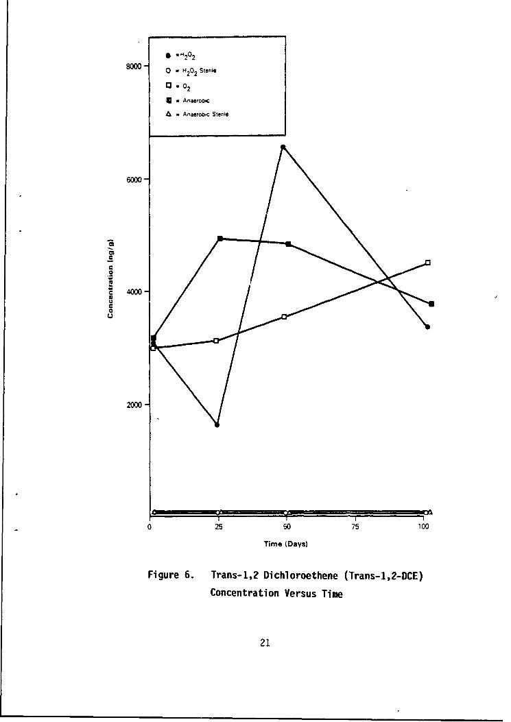
The anaerobic microcosms and sterile controls showed essen-
tially no significant aliphatic hydrocarbon degradation over the 100-
day period. However, anaerobic degradation of tetrachloroethylene
(PCE) (Figure 4) and trichloroethylene (TCE) (Figure 5) occurred
within the first 49 days of the study. During the first 24 days,
concentrations of trans-1,2-dichloroethylene (trans-1,2-DCE) in-
creased in the anaerobic microcosms, followed by a gradual decrease
in trans-1,2-DCE from Day 24 through Day 100 (Figure 6). Decreases
in groundwater concentrations of PCE and TCE and increases in trans-
1,2-DCE concentrations were also observed during the field demonstra-
tion program. The laboratory biodegradation studies, therefore, were
a successful tool for determining the treatability of contaminants
and predicting what would occur in the field. The field results
are discussed in subsequent chapters.
16

* = az20
40 0 = a202 Sterile
o = 02
- Anaerobioc
= Anaerobic Sternk
30-
0 20-0
U
10-
0 25 50 75 100
Time IDays)
Figure 3. Chlorobenzene Concentration Versus Time
18

6 = H20 2
16003-- o = H20 2 Stevie
S.02
S- Anaeroawc
-- Anaerob€c Sterne
1200-
sw
400-
0 25 50 75 100
Time Idays)
Figure 4. Tetrachloroethene (PCE) Concentration Versus Time
19

* = H2 02
1600 O H20 2 Sterile
3 - 02
- Anaerobic
A AnaerobiC Sterile
1200-
* 800-
0 110
U
400-
25 50 75 100
Time (Days)
Figure 5. Trichioroethene (TCE) Concentrations Versus Tim
20
* = 202
"800 o H20 2 Sterile
0 -02
-* Anaerobic
A = Anaerobic Sterile
0
4000-
0
2000
0 25 50 75 100
Time (Days)
Figure 6. Trans-1,2 Dichloroethene (Trans-1,2-DCE)Concentration Versus Time
21

In general, the results of the laboratory treatability study
demonstrated that: (1) in situ microbial populations could degrade
the contaminants present in the soil at Kelly AFB; (2) active cultures
were developed which demonstrated degradation of aliphatic hydrocarbons
(n-alkanes) and aromatic compounds (chlorobenzene) under aerobic condi-
tions and chlorinated hydrocarbons under anaerobic conditions; (3) oxygen
treatment and introduction of hydrogen peroxide worked equally well for
degradation of petroleum-type compounds; and, (4) biotransformation of PCE
and TCE to the lower-molecular weight chlorinated aliphatic compounds,
trans-1,2-DCE and 1,1-DCE, occurred under anaerobic conditions. Chlori-
nated hydrocarbon degradation under anaerobic conditions has been reported
previously in the literature (Reference 15).
2. Permeability Studies
Permeability studies were conducted on soil samples collected from
the Kelly AFB site to determine the effect of nutrient (Restore® 375K)
and hydrogen peroxide (Restore' 105) addition on soil permeability.
Triaxial permeameters were used to determine the permeability of two
undisturbed soil cores. A solution of nutrients, hydrogen peroxide, and
groundwater (collected from Lhe site) was permeated through the soil
samples and leachate was collected periodically and analyzed for
chloride, phosphate, and hydrogen peroxide concentrations. Details of
the sampling methods, analytical procedures, and raw data are given in
Volume I of this report.
Results from the permeability studies (Figures 7 and 8) showed
chloride breakthrough occurred first, followed by phosphate breakthrough.
Phosphate concentrations in the leachate solutions did not exceed 60 to 70
percent of the influent phosphate concentrations. This was attributed
to calcium phosphate precipitation in the soil. Similar effects, i.e.,
22

1.0-
0 Peroxide0.9- A Phosphate
0.8- r3 Chloride
0.7-
0.6-
0.5-
0.4-
0.3-I
0.2
0.1
0.0-Groundwater Groundwater Plus Nutrients and
Only -Peroxide
5x 10-6
LUL
x10-
S1 X 10. 7
:E
0.
--- 5 X 10.-6
lx107 I
5x 10 6 -
1 0 0.0 1 0 2.0 3.0 4 0
Pore Volume
Figure 7. Permeability and Nutrient Solution Breakthrough
for Soil Sample Number One
23

1.0-0.9 0 Peroxide I
0.8 A Phosphate I0.- C .hloride _
0.6-
0.5-
0.4-
0.3 I0.2-
0.1
0.0 -Groundwater j _ Groundwater Plus Nutrients and
Only Peroxide5x 10.6
(II1 X 10.6 I
5 x 101 -SSlope - -0.03
. r = -018
5 x10-61 0 0.0 1 0 2.0 30 40
Pore Volume
F.gure 8. Permeability and Nutrient Solution Breakthrough
Curves for Soil Sample Number Two
24

initial breakthrough of chloride followed by low phosphate breakthrough,
were observed during the field study. Results from these studies also
indicated that permeability reduction of the soils occurred following
addition of nutrients and hydrogen peroxide. This effect was also
observed during the field demonstration project and is discussed in sub-
sequent chapters. The permeability studies also indicated that peroxide
breakthrough was slower than that for phosphate, as was observed in the
field.
D. DESIGN AND INSTALLATION OF TREATMENT SYSTEM
Many site-specific factors were considered in developing a treatment
approach that would best suit the conditions present at the Kelly AFB
site. The variable geology at Site E-1 necessitated a system that could
be readily adjusted to conform to actual subsurface characteristics
within the treatment zone, which would not be known with certainty until
system wells were installed and tested. Circulation of groundwater,
introduction of nutrients, and introduction of an oxygen source were the
necessary conditions for providing adequate microbial activity over a
specific area. A major concern was the probable hydrologic communication
between the shallow aquifer and nearby Leon Creek. The system was designed
to provide a closed circuit operation (containment and recirculation of
groundwater within the demonstration area) to prevent contaminants from
migrating toward Leon Creek. Due to the constraints of site character-
istics and time, the treatment test was performed within a small area of
Site E-1 and not for the entire site. The area was chosen because soil
in the saturated zone had high concentrations of petroleum hydrocarbons
which could be aerobically biodegraded.
After considering several alternatives, it was decided that a
series of injection wells surrounded by pumping wells would best pro-
vide the closed system necessary for the demonstration. Several well
configurations were tested with a two-dimensional geohydrologic model
which simulated groundwater flows. The model assumed a homogenous site
25

and an isotropic aquifer of uniform thickness. The actual conditions at
Kelly AFB were more complicated, limiting the models' ability to accurately
represent site reaction to various pumping and injection schemes. Even
so, the model was useful in determining a site configuration that would
keep water levels stable and minimize the effect outside the treatment zone.
The resulting well system configuration, illustrated in Figure 9,
was constructed at the Kelly AFB site in April and May 1985. The system
consisted of nine pumping wells and four injection wells arranged in a
grid pattern within a circular area 60 feet in diameter. It was designed
so that each injection well would be surrounded by four equidistant
pumping wells 15 feet away. The pumping wells were 4 inches in diameter
and the injection wells were 6 inches in diameter. All wells were 30
feet deep and cased with PVC piping. The bottom 15 feet of the casing
was slotted. In addition, 2-inch monitoring wells were placed one up-
gradient and one downgradient of the demonstration site. Existing Well
CC was used as an additional downgradient monitoring well.
Although biodegradation of contaminants takes place underground,
groundwater circulation, groundwater and chemical storage facilities,
and chemical addition equipment were installed on the surface. Each
pumping well was equipped with a durable, 1/2 horsepower, submersible
pump which was selected to be able to run continuously for the life of
the project. A pump capable of operating continuously for a long time
at the extremely low flow rates required at this site could not be
found. Therefore, it was necessary to punip water from each well at a
much higher rate than needed and return the unused portion to the well.
This was achieved with a dual-valve system located above the well casing.
Figure 10 illustrates a typical pumping well. The release valve was set
to allow the desired amount of flow into the system; the check valve
provided the necessary back pressure on the pump and allowed the overflow
to pass into the overflow line and return to the well. Each pump was
individually controlled by dedicated electrodes that sensed high and low
water levels in the well. When the level of water in the well dropped
26

o0 0
6Q
Im'4-0
- I-(9))
0 cm.r.
0 U-
LO~
/2
27

Flow RateControl Valves
- To Surge Tank
-o Sampling Port
oCompression1I PVC Piping Fittings
Overflow _ Union Joints
Line •
Cntro OvercasingBox
Pump WirePower Electrode Wires
In
S4" PVC Casing
Cement- Benton ite Grout
Bentonite Seal
Upper Electrode-- •Sand
Lower Electrode
4" Submersible Pump * .'
Figure 10. Cross Section of a Typical Pumping Well
(Not to Scale)
28

below a safe level for pump operation (0.5 foot above the intake), the
pump shut off automatically. After the well recharged, the pump began
operating once again.
Once groundwater entered the system, it flowed by gravity to a
central surge tank. A valve at the bottom of the surge tank released
water at a controlled rate into a feed pipe in which the nutrient and
hydrogen peroxide solutions were also introduced. This combined flow
then passed through a section of baffled pipe to facilitate mixing
before it entered a distribution box which divided the flow among the
four injection wells. Flow in three of the four lines to the injection
wells was controlled by valves, while the fourth line remained unob-
structed to prevent a backup of water in the distribution box. The
system configuration is illustrated in Fiqure 11.
Choice of materials was a major consideration in system design.
All materials chosen were first determined to be nonreactive with con-
taminants known to be present at Site E-1 or the treatment chemicals.
PVC was chosen for all piping, valves, and fittings. All connections
were heat-welded to avoid the use of glues, which could have introduced
unwanted organic chemicals to the system. Pumps and electrodes were
constructed of stainless steel. Other plastics that came in contact with
groundwater included insulation for pump electrical wiring. No detectable
adverse effects were found to result from the materials chosen for con-
structing the treatment system.
29

Key:
0 Irlection Wells
o Pumping Wells
0 Monitoring Wells
- Pumping Lines
--- Injection Lines
A Distribution Box
B Surge Tank
P6P7 P8
13 14 M2
® P. o.- -P
--- P9
Ml
Ccc
P4 P. P2 r Elect.ical"L.i Line
CircuitBox
Site OfficeTrailer
Storage Yard
Figure 11. Plan View of System Configuration
(Not to Scale)
30

SECTION III
TEST PROCEDURES
A. DESCRIPTION OF FIELD OPERATING PROCEDURES
For most system operations, one field technician was responsible for
all onsite activities. A field operations manual was developed by SAIC
to ensure that proper procedures were followed at all times. The field
technician (engineer or geologist) was responsible for mechanical opera-
tion of the system and the sampling and analysis program. The following
sections discuss the details of these activities.
1. System Operation
System operation activities included operation and maintenance
of all pLImps, piping, and electrical controls as well as mixing nutrient
and peroxide solutions for gravity injection. Because of insufficient
injection capacity, pumps were operated on a rotational basis. Usually four
pumps were operating at any one time, along with pumping well P1, which was
a very poor producer. The flow rate from each operating pump was recorded
as were rates to each injection well. Nutrient and peroxide flow rates were
set at the specified level and allowed to run while groundwater was being
circulated. Concentrated nutrient solution was only introduced at afew gallons per day and stopped completely in late October 1985. Peroxide
was injected during the entire period of pump operation, with the exception
of the first 2 weeks and several weeks in November 1985.
A daily log sheet was completed each day. This form reported
flow rates, water levels, and other important operating characteristics.
These data were summarized weekly in a report to the project manager.
Maintenance of injection wells required periodic redevelopment which
31

included air surging and hand bailing to clean well screens and remove
fines and precipitate.
2. Sampling Schedule and Procedures
A detailed sampling and analysis program was followed throughout
the operation of the treatment system. Groundwater and soils analyses
were performed both onsite and in offsite laboratories for a number of
physical, chemical, and biological parameters. Table 2 lists these para-
meters and indicates the frequency of analysis for each one.
The field technician was responsible for collecting all of the
samples and performing all of the onsite analyses. Laboratory samples
were placed on ice and mailed by overnight air freight to the designated
laboratory. Strict adherence to site-specific QA/QC and health and safety
procedures were followed during all sampling activities. These procedures
are addressed in subsequent sections of this report.
Sampling for tests performed onsite was normally performed in
the morning so that analyses could be performed the same day. Samples
from pumping wells were taken from the sampling ports located near the
release valves of each well (see Figure 10). Samples of groundwater from
injection and monitoring wells were obtained with a PVC bailer. Soil
samples were obtained using a standard, thin-walled sampling tube (Shelby-
tube). The samples were split once and placed into: (1) two 750 mL jars
for total phosphates, inorganic orthophosphate, hydrocarbons, and priority
pollutants, and (2) four small, sterile glass jars for microbe counts.
Soil sampling locations are shown in Figure 12.
Great care was taken to ensure sterile sampling conditions and
to prevent cross-contamination of samples. The decontamination procedures
followed are discussed in Section III-B.
32
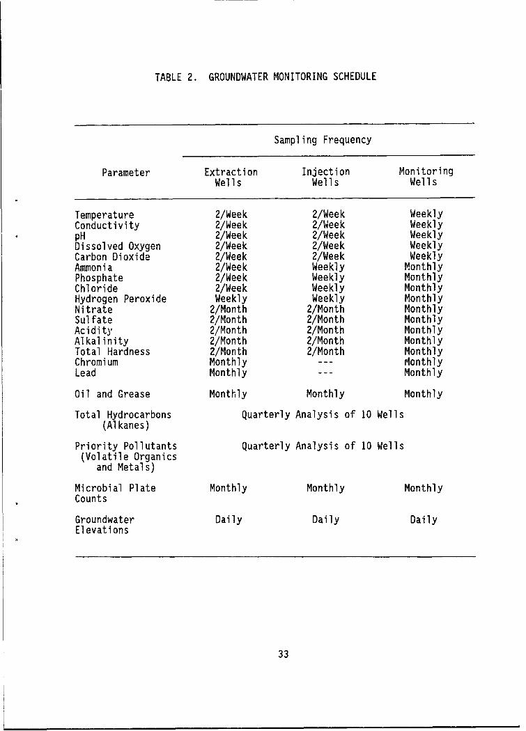
TABLE 2. GROUNDWATER MONITORING SCHEDULE
Sampling Frequency
Parameter Extraction Injection MonitoringWells Wells Wells
Temperature 2/Week 2/Week WeeklyConductivity 2/Week 2/Week WeeklypH 2/Week 2/Week WeeklyDissolved Oxygen 2/Week 2/Week WeeklyCarbon Dioxide 2/Week 2/Week WeeklyAmmonia 2/Week Weekly MonthlyPhosphate 2/Week Weekly MonthlyChloride 2/Week Weekly MonthlyHydrogen Peroxide Weekly Weekly MonthlyNitrate 2/Month 2/Month MonthlySulfate 2/Month 2/Month MonthlyAcidity 2/Month 2/Month MonthlyAlkalinity 2/Month 2/Month MonthlyTotal Hardness 2/Month 2/Month MonthlyChromium Monthly --- MonthlyLead Monthly --- Monthly
Oil and Grease Monthly Monthly Monthly
Total Hydrocarbons Quarterly Analysis of 10 Wells(Alkanes)
Priority Pollutants Quarterly Analysis of 10 Wells(Volatile Organics
and Metals)
Microbial Plate Monthly Monthly MonthlyCounts
Groundwater Daily Daily DailyElevations
33

do0
0 . 0 . CL
C4 4.A
00 u
NI
0 oI
a..
00Fm
4-
t,
.I
4.3
UDU
U 0. 0
U Im
:434

B. DESCRIPTION OF ANALYTICAL PROCEDURES
Soil and groundwater samples were collected periodically during the
field demonstration project to evaluate system performance and treat-
ment effectiveness. A quality assurance project plan was developed
by SAIC to ensure that proper analytical procedures were followed both
in the laboratory and in the field. Details regarding QA/QC procedures
are discussed in subsequent sections of this report. The sampling fre-
quencies for chemical and microbiological analyses are given in Table 2.
The following sections discuss the procedures used for both laboratory
and field analyses.
1. Microbiological Enumeration
Soil and groundwater samples were collected and sent to con-
tracted laboratories for enumeration of total bacteria and hydrocarbon
utilizing bacteria. FMC/Aquifer Remediation Systems laboratory per-
formed the analyses on samples collected from April 1985 through October
1985. No soil or groundwater samples were collected for microbial
analyses during November 1985. Microbial samples collected from Decem-
ber 1985 through February 1986 were analyzed by Biosystems, Inc.
The enumeration methods used by each lab consisted of plating
groundwater or soil solutions on nutrient agar media to determine total
bacteria colonies. The enumeration of hydrocarbon-degrading bacteria
was conducted by incubating the inoculated basal mineral salts agar
plates in dessicator jars supplemented with gasoline. Dilution series
plates were used for all samples to obtain 20-300 colonies per plate.
Duplicate enumeration analyses were performed on selected soil and
groundwater samples as part of the QA/QC procedures. Specific media
compositions and procedures utilized by each contract laboratory are
presented in Volume III (Appendix E).
35

2. Laboratory Chemical Analyses
Groundwater and soil samples were collected throughout the
field demonstration project and sent to contracted laboratories for
chemical analyses. Chemical analyses on samples collected during
April and May 1985 were performed by Aqualab, Inc. All subsequent
chemical analyses were conducted by Environmental Research Group
(ERG). Chemical analyses performed on soil samples included priority
pollutant volatile and metal compounds, total hydrocarbons (alkanes),
oil and grease, total organic carbon, total inorganic carbon, total
phosphorus, and inorganic orthophosphate. Groundwater samples were
analyzed for chemical parameters which included priority pollutant
volatile and metal compounds, total hydrocarbons (alkanes), oil and
grease, total organic carbon, and total inorganic carbon. Field QA/
QC samples included field blanks, bailer washes and duplicates. Con-
tract laboratories performed in-house QA/QC procedures including dupli-
cates and matrix spike additions. QA/QC procedures are discussed in
detail in later sections of this report.
Analytical procedures used for chemical analyses of soils and
groundwater are listed below.
Soils
Priority Pollutant Analysis
Volatile organics EPA Method 8240
Metals EPA 600/4-79-020
Total Hydrocarbons (alkanes) Nonstandard
(See Volume III, Appendix D)Oil and Grease Extraction/EPA 413.2
Total Organic Carbon EPA Method 9060
Total Inorganic Carbon EPA Method 9060
Total Phosphorus ASTM 424
Inorganic Orthophosphate ASTM 424
36

Groundwater
Priority Pollutant Analysis
Volatile Organics EPA Method 624
Metals EPA 600/4-79-020
Total Hydrocarbons (alkanes) Nonstandard
(See Volume III, Appendix D)
Oil and Grease EPA Method 413.2
Total Organic Carbon EPA Method 415.1
Total Inorganic Carbon EPA Method 415.1
All chemical analyses were performed in accordance with the
standard chemical methods listed.
3. Field Chemical Analyses
Soil samples were collected at the Kelly AFB site on a quarterly
basis and a split from each sample was kept onsite for field test
analyses. Soil analyses were performed by the field technician (engi-
neer or geologist) for the following parameters: pH, calcium, iron,
magnesium, manganese, ammonium, nitrate, nitrite, phosphorus, and
sulfate. Analyses were performed using a Simplex Soil Testing Kit
(Reference 18). Instructions and chemicals for conducting the field
analyses were provided with the field test kit. These analyses were
performed to obtain estimates of the parameter concentrations for use in
system operation decision-making and were not intended to replace analyses
performed by contract laboratories.
Groundwater was monitored onsite for tne following parameters:
pH, temperature, conductivity, dissolved oxygen, carbon dioxide, ammo-
nium, phosphate, chloride, hydrogen peroxide, alkalinity, acidity, total
hardness, nitrate, sulfate, lead, and chromium.
At the time of collection, groundwater samples were split once.
One split was immediately analyzed for dissolved oxygen, temperature,
37
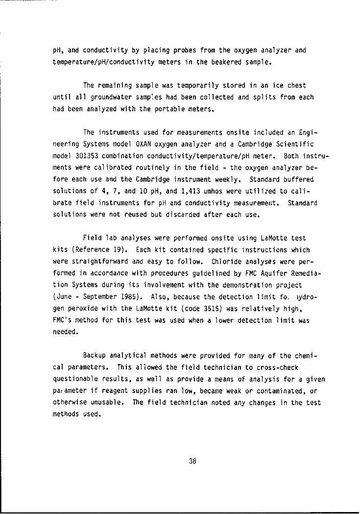
pH, and conductivity by placing probes from the oxygen analyzer and
temperature/pH/conductivity meters in the beakered sample.
The remaining sample was temporarily stored in an ice chest
until all groundwater samples had been collected and splits from each
had been analyzed with the portable meters.
The instruments used for measurements onsite included an Engi-
neering Systems model OXAN oxygen analyzer and a Cambridge Scientific
model 301353 combination conductivity/temperature/pH meter. Both instru-
ments were calibrated routinely in the field - the oxygen analyzer be-
fore each use and the Cambridge instrument weekly. Standard buffered
solutions of 4, 7, and 10 pH, and 1,413 umhos were utilized to cali-
brate field instruments for pH and conductivity measuremer;t. Standard
solutions were not reused but discarded after each use.
Field lab analyses were performed onsite using LaMotte test
kits (Reference 19). Each kit contained specific instructions which
were straightforward and easy to follow. Chloride analyses were per-
formed in accordance with procedures guidelined by FMC Aquifer Remedia-
tion Systems during its involvement with the demonstration project
(June - September 1985). Also, because the detection limit fo iydro-
gen peroxide with the LaMotte kit (code 3515) was relatively high,
FMC's method for this test was used when a lower detection limit was
needed.
Backup analytical methods were provided for many of the chemi-
cal parameters. This allowed the field technician to cross-check
questionable results, as well as provide a means of analysis for a given
parameter if reagent supplies ran low, became weak or contaminated, or
otherwise unusable. The field technician noted any changes in the test
methods used.
38

QA/QC procedures on Hield chemical analyses included analyzing
duplicate samples on a routine basis and analyzing selected standard
solutions with the field test kits. Standard solutions were provided
by Raba Kistner Laboratories of San Antonio and included the following
parameters: chloride, ammonium, phosphate, lead, and chromium. Field
QA/QC procedures are discussed in subsequent sections.
C. SITE HEALTH AND SAFETY PLAN
A detailed health and safety plan was developed to establish site-
specific procedures and was followed for all activities at the Kelly AFB
site. Specific protection levels were established for the following site
activities:
e Routine system operation
e Grouadwater sampling
e Handling of hydrogen peroxide
* Drilling and soil sampling
e Test kit operation.
Protective equipment was maintained onsite to provide EPA Level "C"
protection for at least three persons. In addition, the following safety
measures were taken:
e First aid kit was made available in an onsite trailer
e Fire extinguisher was provided in the trailer
* Eye and body wash kits were made available onsite
e CAUTION and NO SMOKING signs were posted to indicate fire and
electrical hazards
4 Flagging was used to mark trip and overhead hazards
e Emergency phone numbers were posted in the trailer* First aid and laboratory safety charts were posted in the trailer.
39

D. SITE MITIGATION PLAN
A detailed site mitigation plan was aeveloped to establish proce-
dures for monitoring contaminant migration from the treatment area and
develop a course of action for mitigation in the event that significant
contaminant migration was discovered. Monitoring well CC was designated
to monitor contaminant migration. Each new set of results was compared
with historical values to determine if unacceptable levels of any con-
taminant were threatening to reach Leon Creek.
In the event that high levels of contaminants were found in Well CC,
SAIC would report this information to EG & G and the Air Force. A joint
decision by the Air Force, EG & G, and SAIC would then be made as to
whether mitigative action was justified. Immediate action would have
consisted of pumping the entire system at capacity to try to draw ground-
water away from Leon Creek. Several system riodifications were suggested
to permit the system to operate at a higher pumping rate for a longer time
period than planned for in the system design. More permanent mitigative
measures were suggested in the mitigation plan including barrier walls
and an onsite treatment system. These methods were cost-prohibitive and
were to be implemented only as a last resort.
E. SYSTEM SHUTDOWN
The final day of system operation at Kelly AFB was February 17, 1986.
The system was then completely disassembled. All wells were left intact
and locked. The circuit box and electrical outlets were also left on-
site but power was turned off. All other project-related items were
removed from the site.
40

SECTION IV
SYSTEM PERFORMANCE
A. STARTUP
System construction was completed in mid-May 1985. Following con-
struction, pumping tests were performed to determine transmissivity
values for all nine pumping wells. Using the data collected from these
tests, each pump was set to a rate determined from the pumping tests to
result in steady-state yield. Pumping rates were highly variable be-
cause of the heterogeneity of the test site, and the total flow from all
nine wells was only slightly more than 1 gallon per minute because of
low yield of the shallow aquifer. This flow was originally distributed
equally among the four injection wells. However, each of the injection
wells exhibited different permeabilities and the flows were adjusted to
the maximum thdt could be accepted by each well. Groundwater was cir-
culated through the system for several days prior to the introduction
of nutrients so that flow rates could be readjusted and any other pro-
blems with the system could be worked out. Several pumps had to be re-
moved during this testing period to be cleaned, because of fines re-
maining in the wells after development.
Nutrient introduction began on June 7 and was performed for several
weeks before hydrogen peroxide injection began on June 26. The initial
plan was to begin hydrogen peroxide concentrations at 100 ppm in the
groundwater injection flow. Concentrations were then to be increased
by 100 ppm every 2 weeks to achieve a final total concentration of 500
ppm in the injected groundwater. Due to the steadily decreasing flow
rates, however, much higher levels were actually introduced. This is
discussed more thoroughly in Section IV-B.
41

Initially, a system was set up to 'Introduce both the nutrients and
peroxide in a single solution. Set volumes of each solution were mixed
together with water in a 30-gallon drum to achieve the desired concen-
trations. A small chemical feed pump was then used to transfer the
solution at a set rate into the groundwater circulation flow. After
approximately 3 weeks, the system was altered so that nutrients and
peroxide were controlled by separate feed pumps. This change was made so
that the nutrient solution could be injected at a higher concentration
over a shorter time to control precipitation. This problem is further
discussed in Section IV-C.
B. SCHEDULE OF CHANGES OF OPERATING PARAMETERS
Table 3 provides a weekly summary of the major changes made or in-
curred in the operation of the well system with regard to: average
chemical concentrations of injection well fluids, the oxygen source as
hydrogen peroxide (H202), and nutrients (the inert parameter as chloride,
water circulation volumes and rates; and other parameters such as well
" ; the nitrogen
source as NH3; the phosphorous
source as P04);
ground-
workover frequency, days of peroxide and nutrient injection, soil and
groundwater sampling for microbial and priority pollutant analysis, and
field staffing level.
A total of 52,267 gallons of groundwater were circulated over a
period of 259 days, from June 5, 1985 to February 18, 1986. Based on
a 60-foot diameter of the well area, a 10-foot vertical aquifer thick-
ness, 20 percent porosity and a grain density of 162 lbs/ft3, this
volume of circulated groundwater corresponds to a displacement of 1.25
pore volumes. This nominal geometry of the well pattern contains 1850
tons of soil and 42,300 gallons of groundwater.
Nutrient addition to the groundwater was in effect from June 7,
1985 to November 7, 1985. Following November 7, 1985, residual
42

- -- -8 -i -08 ------------
0O z0. 0.d On N -N NN1 . ( 1f Nk o1 -l t ,N N Nr ,r
0 0V)ono
F-0
m ,Y0 N N.- 0 3N. NNNN-r-NN-
LU 0
-2 102 0 0 C ý00 0 a 0 00 00
zi
LUJ43(S "1 0002) r4 0,L^0 o0 ?
""1 07", or-m1- 0
'. .^ M _N4'- 1 y t 2 ;It It .l, 0 t .,c;
0ý C ý C
>- ,2 ý 29z
m >0,
LU 00
N 0 0 0coN V% 0000.0 W00 'p~.0 0 00 c n 0LNQ 'CO)U 00OQN 20 0 4 '0o4 '040
OL *-- cli U'N' 00 -40 Go 0 K 4 p 'D U'~ 0u r0r- N0 o-4N-jý ý000Qm0zN mL
4) C
4C0 4ým C4 N .- r
41 0 r tý 4N w' 0. U' !2 :2 m. 0ý 4 m) LA V0
CID co 000 coDo o c N co 0 ww Q 0 0- m 0 w 0.N 0n00 0. QN4.00 -7Cry18 "0 N Nn 0 y(w mr
'o mS0OS0N 80 N ~ 0 0U~00 ''..0 0 00 0~ 4.4 N 400g0.ls 8ons o nzzlig4A N- 'U0
~ U' 03

nutrient in the groundwater obtained from the production wells pro-
vided the only source of nutrient for the injection wells. During
the period of nutrient addition to the groundwater 'June 7, 1985 to
November 7, 1985) average nutrient chemical concentrations based on
bulk chemical addition were:
# 812 ppm NH4 as nitrogen source
* 1598 ppm P04 as phosphorous source
* 1598 ppm Cl as inert.
The chloride (Cl) is used as a chemical tracer to analyze well pattern
chemical effects as initial groundwater background levels averaged less
than 40 ppm.
The total quantity of hydrogen peroxide added to the injection wells
during the field operation was 299 pounds. Based on a nominal well pat-
tern groendwater volume of 42,300 gallons, a soil mass of 1850 tons, and
an average hydrocarbon contaminant oxygen demand of 3 parts oxygen per
part contaminant, a maximum reduction of 133 ppm hydrocarbon in the
groundwater or 12.8 ppm hydrocarbon concentration in the soil would have
been possible. Hydrogen peroxide (H2 02 ) addition to the circulated
groundwater was in effect from June 21, 1985 to November 7, 1985, and
from December 6, 1985 to February 14, 1986. The average H2 02 concentra-
tion added to the groundwater during the first time period was 1328 ppm,
and 355 ppm H2 02 was added during the second time period. It must be
emp.'asized that this concentration represents what was placed in the
injection wells. No estimate could be made of the actual concentration
entering the formation from the injection well or the speed with which
the hydrogen peroxide decomposed to water and oxygen once in the in-
jection well or in the formation.
The volume of the saturated zone within the test area is used as a
baseline to judge the potential for peroxide to react with hydrocarbons.
It is recognized that hydrocarbons may not have been uniformly distributed
44

over this nominal volume, and certainly were not of uniform concentration
where they did exist. However, using this nominal volume and the peroxide
mass injected in conjunction with a hydrocarbon demand of 3 parts oxygen
per part of contaminant, it is shown that less than 13 ppmi of hydrocarbon
would have been affected over the time of the field test. This level is
an order of magnitude lower than the reported hydrocarbon concentrations.
This indicates that only sufficient peroxide was injected to have impacted
localized pockets of hydrocarbon, either in the saturated zone, or above
it in a comparable 60-foot diameter. However, sufficient peroxide was
present to have impacted contaminants in the water, as the total quantity
of injected peroxide was sufficient to reduce contaminant concentrations
by 133 ppm in the groundwater.
Following the initiation of nutrient and peroxide addition in June
1985, a significant reduction in the groundwater circulation rate
occurred which could not be restored by mechanical cleaning of the
wells. A 93 percent reduction in the groundwater circulation rate
was observed in the first 5 weeks of operation. Less than a 21 percent
restoration of the initial circulation rate was achieved by subsequent
changes in peroxide and nutrient concentrations and 30 mechanical well
workovers.
System operation covered the period between June 5, 1985 and
February 18, 1986, 259 days of 24 hours per day and 7 days per week
operation. System downtime was 5 days, less than 2 percent of the
total time. The field operations staff averaged between one and two
persons per day.
C. MAJOR OPERATING PROBLEMS
From the time the first test wells were drilled, it was clear that low
transmissivity and high variability at the site would cause operational dif-
ficulties. The First significant problem arose during well constrLction.
While flushing the drilling mud out of Injection Well 12, muddy water began
45

to flow out of completed Pumping Well P4 and P5. These wells required
redevelopment. This occurrence suggestel the presence of underground
channeling in that area of the site. However, subsequent results did not
substantiate this assumption. In addition, low permeability made well
development difficult.
Pumping rates for most of the wells were even less than the low
values originally anticipated. These low pumping rates created a pro-
blem with the temperature of the groundwater in the pumping wells. Due
to the small volume of groundwater actually removed from the well, the
temperature of the water was increased by the heat generated by the
pump. As a result, the groundwater temperature in some wells tempo-
rarily reached as high as 100°F.
In addition to the low pumping rates, injection rates were alsofound to be much lower than expected. Several of the wells repeatedly
overflowed and the rates had to be reduced. This created a situation
in which more water was being pumped into the surge tank than could be
placed in the injection wells. To solve this problem and the problem
of elevated water temperature, the pumping operation was switched to
a cycling mode. Alternate pumps were operated for a given time period
and then shut off for an equal period. This reduced the total flowinto the surge tank and allowed the pumps a period of downtime which
controlled the temperature of the water in the well.
After several days of nutrient addition, a considerable drop in theinjection rate was noticed. A thick, white precipitate was also ob-
served in the distribution box. Jar tests were performed to determineif nutrient precipitation was occurring which may have resulted in
clogging of the well screens. Results from the jar tests confirmedthat precipitation of nutrients was occurring and showed that precipi-
tation in the distribution box could be eliminated by increasing the
concentration of nutrients added to the groundwater. This was at-
tributed to chelating agents present in the nutrient solution. Nutrient
46

addition was also switched to a batch mode over a 3-hour period, rather
than continuous addition during system operation, to maintain the over-
all nutrient loading. These changes in the initial design of system
operation eliminated any precipitation in the distribution box. However,
injection rates did not substantially increase. The injection wells
were then manually cleaned, using a large diameter pipe brush. This
removed a large amount of precipitate from each of the wells and re-
sulted in increased injection rates.
After a short period of system operation, however, injection rates
decreased further. It was believed that precipitation of nutrients had
occurred in the formation and resulted in the clogging of pore spaces.
Upon regular cleaning of injection wells, precipitate continued to be
present. Finally, nutrient injection was suspended in late October
1985 to monitor the effects on system performance.
D. WELL PATTERN FLOW EFFECTS
This section discusses system performance with regard to groundwater
circulation rates and fluid communication between wells.
1. Analysis of Changes in Groundwater Circulation Rates
The average weekly groundwater circulation rate is plotted as a
function of weeks of operation in Figure 13. The cross-hatched areas
correspond to periods of declining circulation rates and the shaded
areas correspond to periods of increasing circulation rates. Table 4
lists the changes in the circulation rates over the 14 periods, average
chemical concentrations of injection well fluid, and mechanical work-
overs of the wells.
The largest change in the circulation rate, a decline of 93 per-
cent, occurred in Periods 2 and 3, corresponding with the first addition of
nutrient and peroxide to the groundwater. The subsequent action, including
47

:m .0
V S.-m
a00)
0) i
S-
V) 004c
4-
0
5-
3c
-4 Ad
C0)1-4U
00 0)U..
C)~~~~~ ~ ~ ~ CD C D 4 l a C 0 0 C D C -C) c CD D C 0 C CD Cl C) 0 CD 0 C)
LO Rr 0V 10 0 a% 00 0% %D O 0 yl 0 ~ 0
)18aM J04 942 UO!4LflelJLO pdB *BAV
48

4- LA -
0 L-
Wo 0 0~ -0 0 LC) 9-. m'.
4, ,:- C'.c - U
LO 0 0ý 00 c', 0 OC') C4) CJ
o 0 -4 UC' r. Coo 0 M -q -
.W 0 CDC' 0 0" C14 a).~ ~~~~~ LaC)C) j C") C.)-
=WU
L" w ) 0 ) 0 0 0ý to 0'. C, IN C1 U, r-CD cm 4 c . 0 0D 0 a' C'J r- I Rr m 0 '.< - U)j 0n U,) LO m C' (. -
C., ~ ~ C. 0 D 0 -r a n 0 U) f. 0
0. 0C ~ ~ ý.Ci0,
4.)0LA.) C)L 0 :r r m0.C
U- 0':. 0c
4U~ IV w W
41 > CC-94- C -W WwC-j ~~ 0 ) o 0 cw w Ww a 0w w wcc w. .,n- -c --ý 3C
C. a 4)L c L W ) -W 4 4W a W .V) N 9- > > 0 L
4-.)o C.- 0 0 > a, a, > Tý 4 0 W - > 01) 0w39 0 0- 0 0--0 0 M 0 0-->-4- 0- r- --- C- 0
E >~ 01 >4. ~ . 0Wa VW _ o0a 0 U.- -,h W 0.) w 0iWA. * NC W W- U. - 4. WCW> -> W4&-> 4JI- - >4JL > -.) W C-> FC > t-
u c .- a 00 U-M3 M3 :M0 0 Ca CO 39r -C 00 0 - 00X0---3:--- -0 ~ L- - L,- V 3: -)~ - .- 39 W- * c- -" a - U' *- 04j"oG D41 CO * -"' '4J - - C ~- 4.)' 4.)- 4.)%P
4)-W4 VI%=W0W-C a l- +j 0 w ~>-- oq t- OL 0L . -U UL UL4.) E0> E-) c) 0- , r=)O w .0 >0jV w>=WW C,=d "44) JLOO)0 d)0 O04) )
C L -0) 4- 4- CMtM 4-) ol 4) X > 4.) T)4-a 3) 4-)'~ 3~ 3:3 t :3Z :- g3
0 - C~ 3 00 0 0* 0 C0 0 C ~0' 0 - 0C>4 0 CO CO
U~~~~~~ 0 L.4. >4. 0) 0 ~0 .0 0 ~0 0 '~ -~0~L.4) 04. 0 0 0 00 0- )C)4.) + 4) -3 4-J00 4-)0) O
*) > 0 4J 4-) 41) C4J - 41V - C. ')L - CV * ').t- 4.'J CD Tr ) 0 (J.
w0 3 J )C .G ali m 00 0 C4 C~ .0
0) qr" -- '
0) m 0 aJ M- =. 1- 4.)M- m ý L 4 ~ ~'C0. 0'. . l) 0'. C" 0 m4 C') U' (t-
1-4.) 0 ~~t - ~ ( I 9-. I 4 4 ' 4 .4 .
49

mechanical cleaning of tle wells, resulted in more than a 21 percent re-
storation of the initial groundwater circulation rate (Period 4). It is
likely that addition of both hydrogen peroxide and nutrient contributed to
the permeability decrease. Two likely mechanisms contributed to this re-
duction. The first is peroxide decomposition to water and free oxygen gas
that can reduce permeability due to gas blockage of soil pores. The second
is the exchange of ammonium ions in the nutrient with calcium in the soil
resulting in precipitation of calcium phosphate which blocks soil pores.
As a result of the reduction in permeability during Periods 1, 2, and 3,
over 40 percent of the groundwater circulation occurred during 15 percent
of the operating time.
The highest restoration of circulation rate occurrEd during Period
4 when both peroxide and nutrient concentrations were increased over the
levels used in Period 3. Five well workovers also occurred in this period.
The nutrient solution contained a chemical additive (chelating agent) to
minimize precipitation. Increasing the nutrient concentration in the
distribution tank forced the white precipitate back into solution since
higher levels of the additive (chelating agent) were also present. How-
ever, the response in the well pattern area to increased nutrient concen-
tration could have actually caused further precipitation; the higher
nutrient concentration increased the ammonia level which could have pro-
moted additional release of calcium from the soil. in the distribution
box the calcium concentration is limited as there are no calcium exchang-
ing clays. Another approach would have been to add the stabilizer separate-
ly so that the stabilizer concentration could have increased without in-
creasing the nutrient concentration.
Additional evidence of the impact of hydrogen peroxide injection
on permeability is obtained by comparing circulation rates for Periods 12
and 13. During Period 12 no peroxide or nutrient was added to the ground-
water and the circulation rate increased by 104 gallons per day. During
Period 13 peroxide was added, nutrient was not added, and the circulation
rate declined by 91 gallons per day.
50

The circulating groundwater serves as the transport mechanism to
supply chemicals (oxygen, nutrients) to the cortaminants. The rate of
chemical supply is proportional to the product of the groundwater circu-
lation rate and the concentration of oxygen and nutrient in the injec-
tion fluid. In a system where the key chemical reagents (peroxide and
nutrient) also reduce permeability, an optimum concentration of reagents
may exist where the rate of supply is maximized. Below this optimum
concentration the circulation rate is higher but the rate of chemical
supply is limited by chemical concentration. Above the optimum concen-
tration, low circulation rate limits the rate of chemical supply. Column
treatability testing of representative soils is one method of identifying
levels of optimum chemical concentrations.
2. Fluid Communication in Well Pattern
Fluid communication, based on chloride breakthrough, was achieved
in all pumping wells. The level of this communication varied considerably
between the nine pumping wells and did not correlate with initial permea-
bility. The chloride ion is used as a fluid tracer because concentration
levels in the nutrient were two orders of magnitude higher than background
levels.
Background chloride levels in the groundwater were less than 70 ppm
and averaged 45 ppm for all wells. Chloride monitoring in pumping and
monitoring wells revealed the following:
* Fluid communication was achieved between the injection wells
and all pumping wells, indicating that the opportunity
existed for oxygen and nutrient to interact with contaminants
throughout the entire well pattern.
* The level of this fluid communication was highly variable, as
follows: high for Wells P9, P1, P2 (rating 4); medium for Wells
P3 and P5 (rating 3); low for Wells P6, P7, P8, M2 (rating 2);
and very low for Wells P4, M1, CC (rating 1) (see Table 5 for a
summary of ratings).
51

0 ~ ~~~ -0 -'-. )~3-
a~ 0 0 d) 00 ir 0 4) 010
LLJi
Vd)
00CL
cC ~ 0
Li '-) 0 Q -dididididiidididi*.--d
LU L
LLJ
LU U
IL-0
0iQ: -ý M 3: --- 3: 3
X: .Jý WC ~ C~ c
:3Z E *ý 0 0 0 4)0a0a)LL.I 0
LcLi
-jcc
-4-
CL
0n L-r ( -4 -q -4ý
0.- CL CLa L0 . -a .Li4h l k h* * &:l * q f
352

0 Comparable levels of chloride tracer were obtained in Wells
P9 (highest initial permeability) and P2 (lowest initial
permeability). Figures 14 and 15 indicate the locations of
nelative levels of initial permeability and fluid communica-
tion. Comparison of these data indicates a negative overall
correlation (high permeability-low communication), highlight-
ed by a plot of relative ratings (see plot below). Factors
such as well placement relative to groundwater flow direction
and the presence of clay lenses may influence interwell fluid
communication to a greater extent than well permeability.
4- o o e
3- 0 0
TRACER 2- * o
1- 0
0-0 1 2 3 4
PERMEABILITY
* The chloride levels in the downgradient monitoring well M2
are not in the high and medium levels of communication. This
indicates that natural groundwater flow did not interfere to
a high degree with the circulation of well pattern fluids.
Further evidence of this is the sustaining high levels of
chloride in Wells P1, P2, P3, P5, P9 after day 160 (November
8, 1985) when nutrient containing chloride was not added to
the injection fluid. A strong groundwater effect would have
resulted in a rapidly declining chloride level following day
160.
As a means of evaluating the impact of various changes in operat-
ing parameters on fluid communication, pumping wells with high and
53

•o •a. I. CY
6 aJ
CL•
u
0L.
'4-0
>1
.I-
0 •
000
"0 65 64

0 0 0
6 S i0
0
IL ai
ILL
ci
CIL-
- 0
055

medium communication (P1, P2, P3, P5, P9) and low and very low communi-
cation (P4, P6, P7, P8) were grouped in two sets, and the weekly average
chloride levels for each set plotted as a function of time in Figure 16.
The following can be noted.
* Injection well density in the vicinity of a pumping well
varies considerably throughout the well pattern. Expressing
density as the number of injection wells that are approxi-
mately the same distance from a pumping well; P1 is density
4; Wells P3, P5, P7, P9 are density 2; and Wells P2, P4, P6,
P8 are density 1. On this basis, Well Set P1, P3, P5, P7, P9
would be expected to have higher chloride levels than Well
Set P2, P4, P6, P8 since the former "see" less background
groundwater. Wells P2 and P7 are the exceptions to this
correlation.
* The peaks and valleys of the two sets correlate up to Day
180. Following Day 180, Well Set P4, P6, P7, P8 was pumped
at a 60 percent higher rate than Well Set P1, P2, P3, P5, P9
in an attempt to draw high chloride to these well areas.
This did not occur. In fact, until Uay 248, Well Set P4, P6,
P7, P8 produced essentially background groundwater. This
suggests that a flow barrier may have initially existed or
was formed during peroxide and nutrient injection between
well pairs.
* Before Day 180 (termination of nutrient injection) the two
highest peaks in both well sets occurred between Days 75 and
90 and between Days 135 and 145. Reference to Figure 13 does
not indicate a considerable difference in the behavior of the
groundwater circulation rate in these two periods. These
peaks are most likely a result of flow dispersion of high
injected chloride levels before Day 75 over an area larger
than the nominal area of the well pattern.
* Based on a materials inventory supplied by FMC Aquifer Remedia-
tion Systems, 500 pounds of chloride were added to the ground-
56

IIDt 00
C"! 1l*
CL. CL
CO,
CA
L.6
C) 00
uz'-4
57.

water with the nutrient from Day 3 to Day 64. During this
same time interval 37,558 gallons of groundwater were cir-
culated. If the chloride had been added at a uniform con-
centration, this would be equivalent to 1598 ppm chloride.
When compared with the individual peaks of 1500 ppm in Wells
P9, P1, P2, and 750 ppm in P5, indications are that a con-
siderable portion of the soil volume between these wells and
the injection wells was contacted by circulating groundwater.
E. WELL PATTERN CHEMICAL EFFECTS
This section discusses relative chemical effects observed at the
pumping and monitoring wells resulting from interaction of hydrogen
peroxide and nutrient with groundwater, soil, and contaminants. Chemi-
cal inventories of materials added to the circulating groundwater are
listed in Table 6. Major findings are summarized below.
* Most of the nutrient was taken up by the soil or precipitated in
the groundwater. This uptake varied considerably over the well
pattern area.
* Ammonia loss was less than phosphate. Ammonia breakthrough
occurred in 5 of the 9 pumping wells; phosphate appeared in
only 2 of the 9 pumping wells.
0 Levels of dissolved carbon dioxide measured in the pumping
wells may indicate considerable oxidation of organics by hydrogen
peroxide.
* Well locations associated with low initial permeability appear
to correlate with areas of higher initial levels of ion-exchang-
ing clay.
1. Nutrient (Ammonia and Phosphate) Communication
To assess the relative magnitude of nutrient communication in
the well pattern, ratios of ammonia to chloride (NH3 /Cl) and phosphate to
58

4-) -) (n- Y
4- r r-.(a 0 r-.
C)
0
C0 L
cu Q
>)0D (1 - 0 0
CAq-o 0 0)CLUJ 00 V)M L. a .04--0 0 0D =0 a.) c
= 0A C0 0D CD) O(M *
Q 0 LO 4-) 0
-j0: a 0>.0- Ca. V
ct: (a >) a)
'4-)
CD) Q)L -- L
0 0 A TV) Mr= L
00
4-) L_ ._ a
(2) N -
0. 4-)W 0
Cr, 0).
CEL
LiiI-
>U 4- 1)..00 0. 00 L
-~~C f-A 0 4J4
LL)0 - L Oa M-4 V4- V)*-La 0
mU LL. L.:o >)CUl) 1- 000 a)0 (A 0
>V 0. >a .-C 4- a) ) r-, -
S0L (A M L 0 )(LO.L 1-' UA) L)1
Co1 1.0 Co C4000. 4i
4- cU > u-
LA 0- WA wo 0w) U=W*v n- MoLA-
U,)LL~ -- 00 COLf k-c
59 L>

chloride (P0 4/Cl) are plotted as a function of time for representative
wells where ammonia and phosphate breakthrough occurred (see Figures 17
and 18). Although free ammonia (NH3 ) was not injected into the ground-
water, NH3 is used to report nitrogen (N) levels added as ammonium
ion (NH4 +) in the nutrient. Based on chemical inventory provided by FMC
Aquifer Remediation Systems (Table 6), the respective ratios in the
nutrient supply are 0.48 and 1.0. Since chloride is an inert ion, it is
used as a marker to judge chemical interaction of the NH3 and P04 with
the soil and groundwater. The important findings are presented below.
e Ammonia breakthrough occurred in five (P1 , P2 , P5 , P8 , P9 )
uf the pumping wells and phosphate in two (P 8 , P9 ) of the
pumping wells. No substantidl levels of nutrient were
measured in the monitoring wells. This result, in combination
with the previous finding that chloride breakthrough occurred
in all pumping and monitoring wells, indicates substantial
ammonia and phosphate uptake by the soil and/or precipita-
tion in the soil.
* Ammonia saturation was approached only in Well P9 for the
time interval Day 95 to 185 (September 8, 1985 to December 7,
1985). During this period, considerable loss of phosphate
continued. During the last 30 days of this period, no nutrient
was added to the injected groundwater.
* Based on the maximum values of the NH3/Cl ratio observed
for each well, relative ratings of nutrient communication
are: Well P9 high (Rating 4); Wells P2, P5, P8 medium
(Rating 3); Well P1 low (Rating 2); Wells P3, P4, P6, P7
none (Rating 0). Figure 19 shows the location in the well
pattern area of these relative ratings. Comparison with
Figure 20 does not show a correlation between nutrient and
fluid communication, indicating considerable variability of
nutrient uptake by soil throughout the well pattern.
60

- C-i
~ Ln
E- CO 4.
~L
0
p.-
S.-
1r-
to e
616
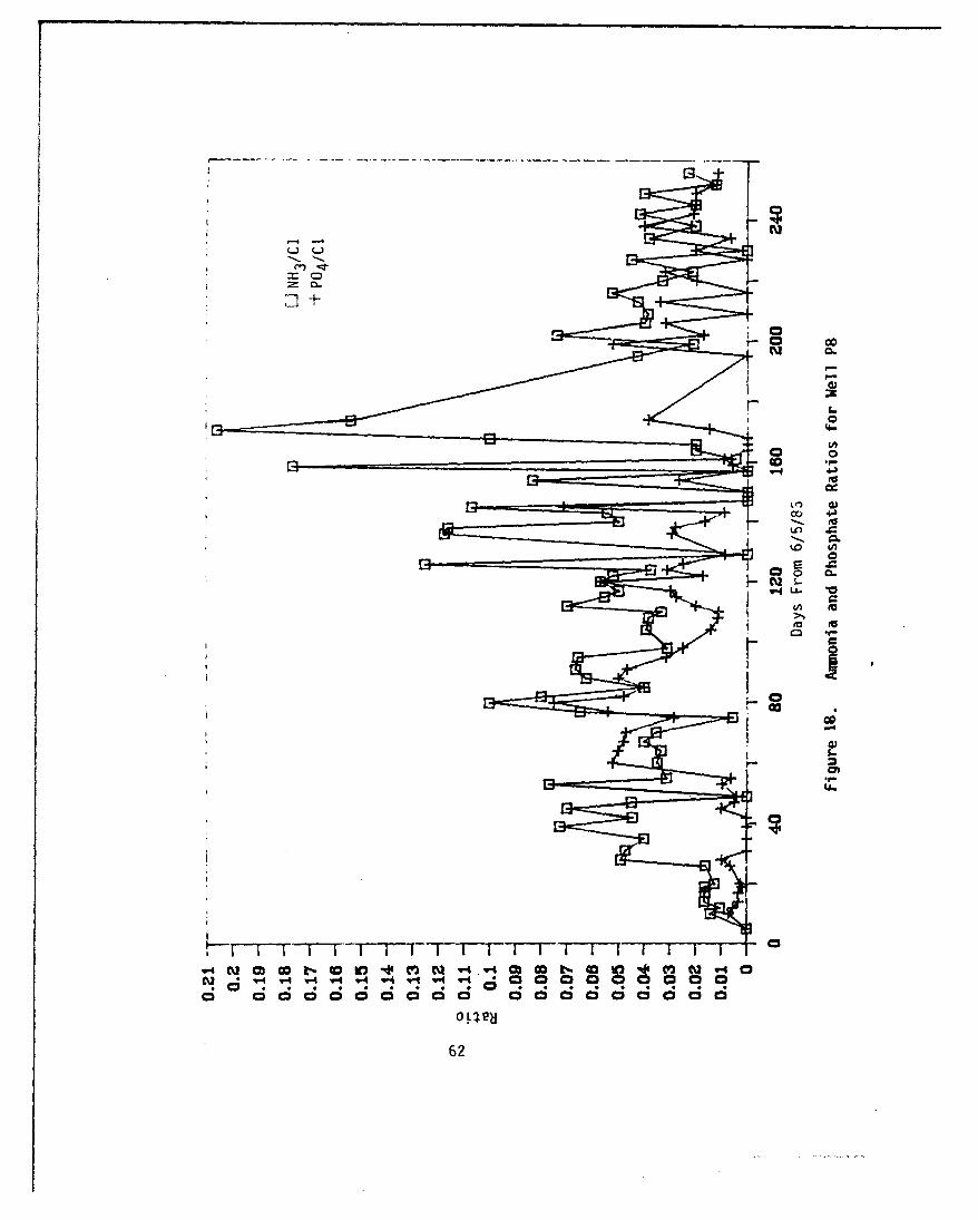
L~ LO
%0 0
0 0.
U-
~C~Cu'4
Cu~~4 w4 9Yw 4 00 00 00
62

00
0o 0
CL
0
cm
0. .C
o 0 °4.1
SlL L.
ILIS00.
0
.9
o 63
00
s 00
0 ba
63

CL
4-3
M 4J
om 0
L.
64)

Calcium-axchanging clays present in the soil could account for
a substantial loss of both ammonia and phosphate from groundwater, re-
sulting in a reduction in the soil permeability. The calcium ion exchanges
with ammonium ion (NH4 +) in the nutrient (nitrogen source, expressed as
ammonia). The calcium ion then reacts with nutrient phosphate to pre-
cipitate calcium phosphate. This precipitate can reduce permeability
by clogging pores in the soil. This reaction would proceed until all
the calcium-exchanging clays were saturated with ammonium ion. This
mechanism is discussed in the following paragraphs.
# The net loss of phosphate relative to ammonia is 1.85 parts
P04 per part NH3 according to the following reaction equations:
Ca-clay + 2NH 4+ .-- -- > (NH4 )2 - clay + Ca++
Ca++ + (2/3) P04 ----- > 1/3 (Ca) 3 (P0 4 ) 2 J precipitate
The ratio in the nutrient was 2.08 (see Table 6). Since this
ratio is larger than the 1.85 ratio associated with precipita-
tion, phosphate breakthrough comparable to NH3 would have been
expected. This did not occur, indicating that a considerable
portion of the phosphorous in the nutrient was not supplied
in a stabilized form. Calcium initially in the groundwater
could also precipitate phosphate.
* The cation ion exchange capacity (CEC) for a Kelly AFB soil
sample, reported in Table F-6 of Volume I is 41.3 milliequiv-
alents per liter of soils of calcium and magnesium (primarily
calcium). Based on this value, an equivalent ammonia uptake
at saturation of 270 ppri. tased on soil) would be expected.
This translates to 988 pounds of ammonia for a well pattern
60 feet in diameter, 10 feet thick, and with 20 percent
porosity. Based on the materials inventory for NH4 in Table
6, only 240 pounds of NH3 were added to the groundwater, 24
percent of the saturation value. The fact that on the average
only 24 percent of the potential ammonia uptake was supplied,
that only one well, P9, at one point approached saturation, and
that not all wells of high fluid communication had high
65

ammonia breakthrough indicates a highly variable exchange
capacity throughout the well pattern.s The concentration of ammonia in the injection fluid is likely
to affect the amount of ammonia uptake. Well P9 had thehighest breakthrough of nutrient. The ammonia-to-chloride
ratio (averaged on a weekly basis) is plotted as a functionof time in Figure 20 for both P9 and the average of injec-
tion wells. The two ratios show correlation except for weeks4.5 through 13.5. In this time period, the highest concentra-tion of nutrient was added to the groundwater. The flat or
slightly declining response in P9 fluid in this time interval
suggests an increase in uptake of ammonia by the soil at a
higher injection concentration.
2. Hardness Changes in Circulated Groundwater
The hardness of the circulated groundwater should provide a rela-
tive marker of those areas of high ion exchange sites since hardness is ameasure of dissolved calcium and magnesium (Figure 21). Relative ratings
of hardness are: Wells P1, P2, P6 high (Rating 4); Wells P3, P7 medium(Rating 3); Wells P4, P5, P8, P9 low (Rating 2); Wells M2 and CC, very
low (Rating 1); and Well M1 none (Rating 0). These are summarized by
well location in Figure 22. Comparison of initial well permeability andhardness ratings indicate a negative correlation. This suggests thathigh levels of ion exchanging clay could be a contributing factor to low
initial permeability. For future tests, CEC capacity measured on soilsamples obtained during site investigation, as well as petrographic
examination of the soil for clay, could be used to provide an initialmapping of permeability. Consideration also should be given to thepossibility that high clay content could concentrate contawiination.
66

Ot~)
, L)
'0 a,Cý co
> > > >
-)
I~~~A 0 ' I -
W4
9
0
-0
vK7 inZ 7
67

00
afa0 .1m
0 LL.
x0
E
5u 0 0
0b
68

4 - O 0 0
3- o 0
HARDNESS 2 - Oo O0
1-
010 I 2 3 4
PERMEABILITY
Considerable quantities of white precipitate, identified ascalcium phosphate, were observed in the distribution tank. This resultedfrom calcium-enriched groundwater mixing with nutrient phosphate in themixing tank. Indications of this effect are noted in e decline in hard-
ness levels of the injection well groundwater after Day 60 (see Figure 23).
Prior to Day 60 the hardness levels rose from an initial low
background level. One explanation is that the calcium exchanged from thesoil exceeded that amount ot phosphate available to precipitate the
calcium. This excess calcium appeared as an initial increase in hardnessAs the test progressed, phosphate concentrations in the injection wellswere increased to a maximum level of 3729 ppm between Days 59 and 73
(Table 4, time interval 5). The combination of increased calcium fromthe pumping wells and increased phosphate addition could have resulted inphosphate precipitation in the mixing tank which would reduce the hardness
of the injection water. Large reductions were then made in the quantities
of ammonia and phosphate added to the injection wells (see Table 4).
This would reduce the source for calcium generation and the source forcalcium precipitation. The hardness would be expected to return to
background levels (250 ppm).
3. Carbon Dioxide (C02 ) Production
Field measurements of carbon dioxide (C02 ) dissolved in circu-
lating groundwater were obtained after November 13, 1985 using a La-
69

00
10
E -0
'0 -.J,S- 0)
>- w
CD (D Cl CD
CD ~ ~~ LO CDZ n 0L
700

Motte field test kit. Figures 24 and 25 plot CO2 levels versus time
in pumping, monitoring, and injection wells.
The lowest C02 levels before Day 220 were detected in Well M1
and the injection wells. M1 was the upgradient monitoring well, thus,
the initial C02 levels most likely corresponded to background groundwater
levels resulting from calcite solubility. The injection well groundwater
has been recirculated and thus exposed to the atmosphere. In this process,
dissolved CO2 escapes to the atmosphere and reduces the C02 level in the
liquid phase. This effect was demonstrated by controlled tests and is
discussed in Section IV-J.
Prior to Day 180, with the exception of Well M1, CO2 levels in pump-
ing and monitoring wells ranged from 100 to 200 ppm. This was five to 10
times higher than the CO2 levels in the injection wells, which indicates
a net gain of C02 as groundwater is circulated in the well pattern.
A net increase of 100 ppm CO2 cannot be attributed to calcite solu-
bility in water, which is 7 ppm, or to oxidation of organics based on the
solubility of atmospheric oxygen which is 9 ppm. This increase occurred
during the production of 35,694 gallons of groundwater and is equivalent
to a removal of 29.7 pounds of CO2 from the subsurface environment. A
discussion of the most likely sources of this CO2 follows.
Reaction of oxygen with organic carbon is a potential source of CO2 ,
resulting in a consumption of 21.6 pounds of oxygen, which is equivalent to
15.5 percent usage of the oxygen contained in the injected hydrogen
peroxide. At a usage factor of 3 parts oxygen per part organic, this
would result in a 2 ppm reduction in soil contaminants or a 21 ppm reduction
in groundwater contaminants. As will be discussed in Part G of this section,
the latter (21 ppm groundwater) is comparable to the maximum level of
23.9 ppm volatile priority pollutants concentration measured in Well CC
in June 1984.
71

00 u
oc
.94-
c~0ca
co ca 0 wm w w m -1w 4 4 W
P~c uz-)
72-

C,,j i to0
X CL CL C
+ c~x
0L
cc,
0 4 c w cc0 CID cc AC~l c ev m V- V-1 -4 v4 V\
ZOC) uzd
73o

Reaction of acid with calcite (CaC0 3 ) minerals in the soil is also
a possible source of CO2 . This reaction requires in situ generation of
acid, since the calcite is attacked by acid to produce CO2 according to the
following: 2H+ + CaCO3 --- > Ca+ 2 + CO2 + H2 0. The quantity of CO2 produced
would require a solution with an initial pH of less than 2.5. As will be
shown in Section V-D.1, groundwater from pumping wells was considerably
lower in pH than the groundwater in the injection wells, which indicates
in situ acid generation. One mechanism by which this acid could be
generated is the oxidation of NH4 , a constituent of the nutrient, accord-
ing to the following reaction: NH+ 4 + 202 --- > NO- 3 + 2H+ + H2 0. This
reaction would consume 43.2 pounds of oxygen to produce enough acid to
generate 29.7 pounds of C02, which is equivalent to 31 percent use of
injected peroxide. A net consumption of 11.4 pounds of NH4+ would result,
which is a small fraction of the injected NH4+. This reaction would also
result in the production of 41.9 pounds of nitrate (N03 "), which represents
an increase in concentration of 141 ppm in the groundwater. No consistent
increase in nitrate is observed in the pumping wells. To maintain this
reaction mechanism for C02 generation another reaction must occur to
remove nitrate. This denitrification can result by interaction of organic
carbon with nitrate according to the following equation: 5/4 organic
carbon + N03- --- > 1/2 N2 + 5/4 HCO3" + 1/4 H+ + 1/2 H2 0. This would
consume 34 ppm of organic carbon in the groundwater or 3.3 ppm on tht
soil.
Another potential source of CO2 is associated with the shift in
carbonate equilibrium resulting from the pH reduction in the ground-
water. As the pH of the groundwater drops from 7 to 6.5 or 6, CO2
increases as the dominant form of carbonate. Just prior to the start
of C02 measurements, the DH measurements in the high level CO2 wells
(Injection Wells and M1) were approximately 7. It is likely that carbonate
equilibrium plays an important role. Several acids were, or could have
been, produced. These include nitrate (oxidation of ammonia), fatty
acids (biosurfactants), and carbon dioxide (biodegradation or chemical
oxidation).
74

Another mechanism that could produce acid in situ is the reaction of
oxygen with trace quantities of sulfides, such as pyrite (FeS 2 ), according
to the following: FeS2 + 3.75 02 + 2H20 --- > 2S04- 2 + 4H+ + FeOOH and/or
+ 1/2 Fe2 03 . This reaction would consume 40.2 pounds of oxygen (29 percent
of the injected peroxide), resulting in a 65 ppm rise in sulfate (SO4-2 ) in
the groundwater, and form hematite (Fe 2 03 ) and/or goethite (FeOOH). Sul-
fate increases were observed in the pumping wells, although not consistent-
ly at a 65 ppm level. In addition, both hematite and goethite were
identified as principal constituents of the sediment produced in Well P7
(Volume III, Appendix A). The significance of this reaction is that it
does not result in any reduction in organics.
Based on the previous discussion, the quantity of CO2 produced
from the pumping wells would account for no more than 31 percent of the
injected peroxide. The remaining 69 percent of the oxygen could have
reacted in one of the following ways.
0 The oxygen could have vented vertically in an unproductive
manner. A 10-foot water table applies an absolute pressure
of 1.3 atmospheres to the groundwater in the soil. At this
pressure, oxygen has a solubility of equivalent to 89 ppm
H202. Based on an average H202 injection concentration of 1000
ppm, 91 percent of the oxygen content is not soluble when
peroxide decomposes.
# Reactions outside of the area of the pumping wells could have
occurred.
e Reactions could have occurred with nonorganics such as metals.
* Incomplete oxidation may have resulted.
Initial ratings (prior to Day 180) of CO2 levels in the pumping
and monitoring wells are: Wells P9, M2 high (Rating 4); Wells P1, P2,
P3, P4, P5, P6, P7, P8, M2, CC medium (Rating 3); Well M1 very low (Rating
1). Figure 26 indicates relative ratings by well location.
75

U
o
a
0
c-S..
CLL
So-
0
*_0
I-
S00.
0 -
iti
00
j >
0000 ob06 76

Variations in CO2 levels between pumping wells are considerably
less than variations in chemical and nutrient communication. A possible
explanation is that peroxide decomposes in the soil to free oxygen gas
and water. This mixture reduces flow in the higher permeability zones
relative to the lower permeability zones which results in a flow smooth-
ing. Free gas can also "finger" through the groundwater and reach con-
Laminated areas prior to the arrival of large quantities of injected
liquid.
The "fingering" of gas refers to an instability that results in
two-phase flow (References 20, 21). Gas, having a lower viscosity than
water (a higher mobility), will tend to move more rapidly under an applied
pressure differential than the water. Gas aphrons are produced under
special conditions to overcome this instability. In the oil industry,
nitrogen and carbon dioxide gas are injected into oil reservoirs to
displace oil. Special conditions must be used to prevent that gas from
fingering through the reservoir fluid instead of displacing it.
It may be possible to use dispersions of oxygen gas bubbles and
liquid to achieve a higher average level of contaminant reduction within
a well pattern area of variable permeability.
Wells P2, P5, P9, and M2 show a declining trend in CO2 with time,
while Wells P1, P3, P4, P6, P7, P8, and CC show a more uniform production
trend. Since hydrogen peroxide, averaging 355 ppm, was added to the in-
jection fluid from Day 185 to 257, a substantial portion of the CO2 reduc-
tion in the first set of wells is prohably associated with depletion of
contaminants. Peroxide breakthrough was observed in Wells P1, P2, and P3
after day 234 (20 ppm in P1, 10 ppm in P2, and 40 ppm in P3).
4. Metals Changes in the Soil
Assessment of changes in soil metal values are based on the data
listed in Table 7, which correspond to soil borings and groundwater
77

co .0 CD 00 Lfl) O en CJ CD 0U4 v4'. c4V 4
00 . - L C) 0 C\J Bq.0 a). .- D -~ I a -C U,, C~
-v v CUv U4
m 0 0)
AC %. 00 en .o 0 400 a~ 0 cUUc00 -4 m .;) 00 .-4 02..
U 2 00 co 'O CD \CO C\J M 4 Ca. a% %0 -4 C2U' N 'q)-r 0e
-~~~- *. c 4U)2 2
L~ .20COCO0 0 0o 0) en 0 .co. I) 2. CDJ CJ U2 0 v t- -. L.C~~
CDv 4 vv 04 0 0LA- LA- LA-A
2/) (D k .0 0- m~ 0)COJ V; 0 v\ 0 4 V 4 L L
2 I V, -4 Vý V VC 00
0: 'U C\
-r 00 CD. 0) ql C) m 0DC.V -4 V4 v 4D:
>1 1- 4 V~ -4 m 01
a. CU'.
LL- - -L ) D C 0 L
U, U,
V/) IO di 0 0 0 CL~0. 4D *-4 V Vu
o: .'r VSa V- Co C. -ooc(I) (A V- - -
01 0 0 2 h 1 0 B toa0. V) ul) COO 0) () 01 0O0U
co 0V 4 C', f(wr() Cm. 'U -4
C L.LL. Ln 0n (4) LO L ) kD 0 0n uO0L
V0 Vo co C'. co c 0co 0 C) C) toL) .
-ý 11 -- I- --- 14..( C
-1Ci m 1C D4 CCD - 41 Cý >4 m, 0fa -' U, %, -- CEC<
V) wr' Ec r- 00.u)MCICD 2.OC -4 0. O
CAL/ u IAC on co.4- = >, fa V) ~ V) 0)
'U 0 0 .- C , 'U U
0/ .)f
B- u~W 0)'78

0r0%0 0 j
C-~
< 0D rn q~ 0 w qw 0 C.
N ~~~-4 ii O
0n0C D 0 m 0 "t C) V) (A -
u 1 N - 4 -4 V -4 V 1-4
o~~~r W400 0 , 0
LL C'D V 4 V .4 N ' C')j
VN V) V) V-
0.i L. _._ -- -4L-
'. N0
V) LA- Ii LA W
(I) > -
CD LI) '.0 4
C, C*4 -' D 0 0D 0 LC) Id ') al 0 0 ot 0 N~ a I
C6 0 ,-4 14 V 14 V I
LA- Oi
0 co Nm m 0 0D 0D 0D LO DCD N -4r 0D 04 co 0
V) -4 V 4
0~ m__ _
00 0 W 0 01 00 0L U,
V) Cf E m.- -i - C1 A
0e 0 0 ) 0 060C0.C '.0 E w-.0 0 ~ I 0
C.) *1 -4 1; V V n n
L. -4 -r _ _:_- -" a)4 C00t0 -j cm 3D cc c cco-,0A
0. N C) LC (11 0n 0IV )0
80) u,0.l) L n oL UlL0co co 00 co 00 0 0 oc C ) o(
0.4.) -i o 0to .- 0 di trc r1
m m 41I 0 "' ) .
V,4) qwC' r,C/ UL# ell 'Ui 4 -lj ~'U CD. - C'f 'IJUj ** C* -~ M 44f
r-4~ C74. Sa0 '-'
U, , , , , L) .0UU, .. O79C

samples obtained from the well pattern area before, during, and following
peroxide/nutrient addition to the groundwater. In addition, a sediment
sample obtained from a flow line at production well P7 was analyzed for
heavy metals. Chemical analyses of the samples were performed by the
three laboratories listed below:
SAIC's La Jolla, California laboratory analyzed the microcosm
samples (Table 7).
* Aqualab analyzed the soil samples collected in April 1985.
TMA/ERG (formerly ERG) Ann Arbor, Michigan, analyzed the soil
samples collected in July and December 1985.
* Analysis of metals by TMA/ERG for the February 1986 sampling
are not shown because an error in the method of analysis was
identified which invalidated the measurements.
* Duplicate samples from the February 1986 sampling were sent to
the U.S. Bureau of Mines (USBM) Twin Cities Research Center for
metals and petrographic analysis. Results for individual sampling
locations are provided in Table 8, averages and ranges are shown
in Table 7 for comparison with previous sampling times. The USBM
separated the fine grain material from the bulk of the soil on
which the chemical analyses were conducted [Rows (1) and (2) in
the tables]. Row (3) is a calculated bulk average which assumes
no metals are present in the +14 mesh size.
Although anomalies exist, specifically between the TMA/ERG and USBM
analysis, indications are that metals appear to be mobilized from the
soil. A specific mechanism of mobilization and transport has not been
identifi ed.
80

0 0 (ý) 0 0 C C 0P-4 ~ ~ ~ ~ ~ dj "( N L V C4 r 4 u') Nl
0 000
- " C1 m E - 4 .4 ~ .vU v IV v I. I. v v v V V V V V
LA.J CD 0 0 00.29 0 En 0 0 E 0 0 0 0 0 0D 0D 0 v
v v v V v v I. V V V I V v IV
Ed ~ 00 0 0D 0 0 0mU 0 E 0 0 0 U') 0 0 CD 0 0o V 0D 0 R4) N4 CV co .. -q - -4 m) I- E ql .. 1- m
-i v v v .4 V V V v v v . V \'
0l 4) 0 0 n 0 M(% cli 0n En 0 0 0 0n 0 C.4 0 m
v 0 V~ .4 Nv -4 'A4 4t -1 .4
LIj c. * 0 %0 0 m 0 0 m (cc c 0% 0 04 - C.,4 0 00 m v 0 0 ?Oi 0 0t 04
)4 0- I" M~ C4 -4 v m0 en co Nq 0n 00 00
0 L)
C) CD
E P-4 m~ -V -4 - - - 0 %0 - -E C.)Cv V V V V V Ve V V V Ne V V"VV I
= EE
= ) 0 00 0D 0O 0 0* 0 004,4 C '4 0o -W E -Ei m -l 14 N ~ N- .- 4 C-4 r- a
C- V V N V V V V V V VC
C CU 4jc* 0 n M m I
(A a. (Al EUc
ý4f C~
co 00 co c000 -1 1
w IE co.E -oco-W --t
m. I..'C1
oyC~
En 40 0 4081

Table 9 summarizes the results of trace metals analysis corre-
sponding to the laboratory microcosm study. Note the following:
* The shaded numbers refer to antimony concentrations in the
water (50 ppb level) and soil (50 ppm level) prior to treat-
ment. The circled numbers correspond to water (5 ppb level)
and soil (<0.5 ppm level) corcentrations after 49 days of
treatment with hydrogen peroxide.
* The treatment resulted in a 100 to 1 reduction of antimony
in the soil, but no subsequent rise in antimony in the water
phase occurred. This effect parallels the field results.
* A possible explanation for this is that the antimony was
mobilized as a fine particle in the water phase, and the
water phase following treatment was decanted from the soil
and filtered prior to chemical analysis. If this occurred,
then no antimony increase would be measured in the water
phase following treatment as was observed.
Metals changes in the soil before and during the system operation
are summarized in Table 7. Column A is the average of multiple samples,
Column B represents the range. Samples taken from April 22, 1985 to
April 26, 1985 were collected before nutrient and peroxide injection. A
summary discussion of the data fcllows.
Changes in metal concentrations corresponding to the Aqualab and
ERG analyses indicate the following:
Antimony reductions are the largest and most consistent
with increasing time. These reductions correlate with the
laboratory microcosm studies.
Cadmium, nickel, silver, and thallium also show consistent
reductions with time.
82

a%
Lo C,, r'ý -. 4 0
oo
CM cd Cm 0
CLL
LLjJ
0Lj~jck:0
0
L.0 0.
-j ON (V V) r
1 0 CC, -ý LA t- a) 0ca .4r LO ~ Q C,0f.
LAJ u'* * . * v
0 0 4w -50
LLJL u W d
Q C') Lt- EI LLJ0 0 0 m
V) co -0-a. -
LU ..- 'C) 0 0 0 (U t XC)L r-. CD N
L 0
'-0 -4) ' N icm
4- 4 > ) 0L
dCo CD. a 0
vv Lfl4
to >., ZCLL ý
L) CD 0 0 c
-c -vr L f
83

* Arsenic, chromium, copper, lead, and zinc changes do not
indicate a consistent change with time and may reflect varia-
tions in initial metals distribution over the wellfield area.
Comparison of USBM analyses of samples obtained at the end of the
field test with ERG analyses of prior samples indicates the following:
Antimony and cadmium levels are not considerably different
than the 04/22/85 to 04/26/85 levels present before peroxide
and nutrient were added to the groundwater.
* Copper, chromium, and zinc appear to be concentrated in the smaller
size soil grains at concentrations that exceed the initial
average measured on the soil prior to field testing.
The above are based on the measurements obtained on the lower
sized fraction of the soil, in which higher concentrations of
metals might be expected (Rows (1) and (2) in Table 7). If
it is assumed that no metals are contained in the +14 mesh
size fraction (Row (3) Table 7), reduced concentrations of
antimony are indicated.
The USBM analysis of the sediment obtained from Well P7 indicates
significant levels of antimony, arsenic, chromium, lead, and zinc. The
concentration of these metals in the sediment, except for chromium, is
much higher than in the soil. The USBM also conducted a petrographic
(microscopic) analysis of both the soil and sediment and observed that
similar clay and calcite mineral particle sizes and shapes were identifiedin both the soil and sediment. This result, in combination with the pre-
sence of metals in the sediments, suggests that circulating groundwater
appears to entrain soil particles which may contain metals and transport
them to the pumping wells. This process could be enhanced by surface
active chemicals initially present in the soil or formed by biodegradation
of organics.
84

The USBM petrographic analysis also identified significant varia-
tions between the oxidation states of iron minerals in the soil and P7
sediment. Iron in the soil is principally ferrous, while iron in the
sediment is ferric. Three possible effects can be associated with this
finding: (1) groundwater entrains and transports ferric minerals, (2)
hydrogen peroxide oxidizes soil ferrous material which precipitates at a
high pH as ferric compounds, which are then transported by the.groundwater,
and (3) ferrous iron contained in the groundwater, when contacted with
air on the surface, is oxidized and precipitates at a high pH as a ferric
compound such as ferric hydroxide which was detected by the USBM to be present
in the surface sediments. The second effect will impact peroxide consump-
tion by soil.
Oxidation of metals by hydrogen peroxide is one possible method of
initiating metals mobilization. The groundwater pH is too high to maintain
oxidized metals in solution and they would likely precipitate as oxides
which could then be transported by the circulating flow. The initial
oxidation state of the metals was not measured. Had the metals initially
existed in a reduced state the oxidation process could consume a con-
siderable fraction of the oxygen content of the peroxide and would not
then be available for aerobic interaction with organic contaminants.
Based on the concentration of the metals (excluding chromium) contained
in the soil prior to peroxide and nutrient addition, it is estimated that
the oxygen demand is equivalent to 20 ppm hydrocarbon in the soil or 208
ppm in water (see table below). The following discussion presents a
calculation of the maximum possible oxygen demand by metals oxidation.
These calculations are based on the average values given in Table 8.
ppm ppm 02
Metal Reaction Metal Demand
Sb Sb -- > Sb2 03 170 33.5 (White)
As As -- > As4 06 4.3 1.4
Cd Cd -- > CdO 5.1 0.7
Cu Cu -- >Cu2 0 6.3 0.8
85
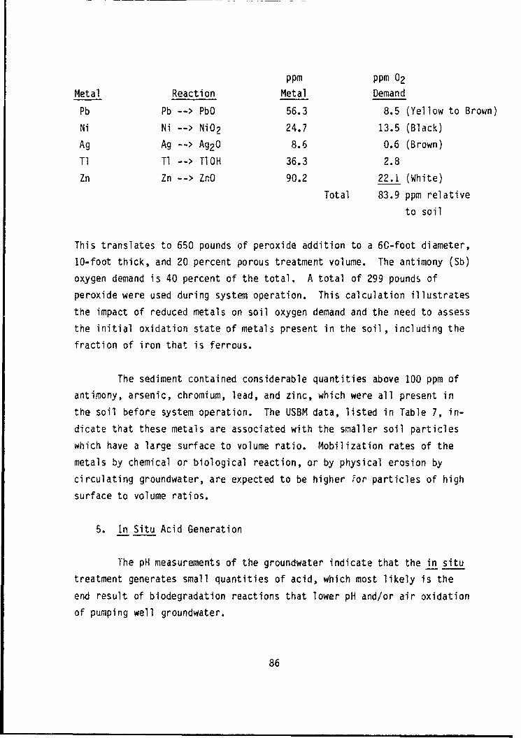
ppm ppm 02
Metal Reaction Metal Demand
Pb Pb--> PbO 56.3 8.5 (Yellow to Brown)
Ni Ni -- > NiO 2 24.7 13.5 (Black)
Ag Ag -- > Ag2 0 8.6 0.6 (Brown)
Tl Tl -- > Tl0H 36.3 2.8
Zn Zn -- > ZnO 90.2 22.1 (White)
Total 83.9 ppm relative
to soil
This translates to 650 pounds of peroxide addition to a 6C-foot diameter,
10-foot thick, and 20 percent porous treatment volume. The antimony (Sb)
oxygen demand is 40 percent of the total. A total of 299 pounds of
peroxide were used during system operation. This calculation illustrates
the impact of reduced metals on soil oxygen demand and the need to assess
the initial oxidation state of metals present in the soil, including the
fraction of iron that is ferrous.
The sediment contained considerable quantities above 100 ppm of
antimony, arsenic, chromium, lead, and zinc, which were all present in
the soil before system operation. The USBM data, listed in Table 7, in-
dicate that these metals are associated with the smaller soil particles
which have a large surface to volume ratio. Mobilization rates of the
metals by chemical or biological reaction, or by physical erosion by
circulating groundwater, are expected to be higher ,or particles of high
surface to volume ratios.
5. In Situ Acid Generation
The pH measurements of the groundwater indicate that the in situ
treatment generates small quantities of acid, which most likely is the
end result of biodegradation reactions that lower pH and/or air oxidation
of pumping well groundwater.
86

A summary of pH variations is shown in Table 10. The lowest pH
value measured in all wells prior to addition of peroxide and nutrients
was 6.4. The groundwater in pumping wells shows a higher incidence of
pH values less than 6.4 than those in injection wells. Well M1 (up-
gradient) has a lower incidence than M2 and CC which are the downgradient
monitcring wells. A survey of the data also shows the period of lowest
pH (pH 6) occurred from September 12, 1985 to November 4, 1985.
6. i'onitoring Groundwater Nitrate (NO3 )
Nitrate can be produced by oxidation of NH4 + in the presence of
nitrifying bacteria. A 50 ppm increase in NO3 would produce sufficient
acid to reduce the pH to 2.8. This reaction would also consume 110 ppm
H2 02 . The low frequency of NO3 concentrations above background and the
fact that the elevated levels in Well P4 occurred prior to the time of
maximum acid generation indicates that either this reaction was not a
dominant factor in the process or both nitrate and acid were rapidly
consumed by organics and calcite.
7. Monitoring Groundwater Sulfate (S04 )
Table 11 summarizes the groundwater sulfate concentration measure-
ments. The largest sulfate value measured in groundwater prior to peroxide
and nutrient addition was 65 ppm. The top portion of the table lists
those wells in which sulfate concentrations above background were measured
by increasing frequency of occurrence. The bottom portion of the table
lists average background sulfate concentrations and average sulfate con-
centrations during treatment for various well groupings.
The concentration of sulfate in Well P2 is consistently above back-
ground, suggesting that a small quantity of sulfate production is occurring
in situ. Potential sources are oxidation of trace sulfides, such as pyrite,
which would also produce acid, and/or increased solubility of any anhydrite
87

TABLE 10. SUMMARY OF pH VARIATIONS
.Averae PH ValuesDays Time Frame I W'ells PWells M1iWell M2 Well CC Well
BeforeTreatment 7.2 >7 7.2 7.2 No Data05/23/85
17 06/17/85 6.8 7.1 1.2 6.7 6.7
19 06/19/85to to 6.9 6.3 6.8 6.4 6.655 07/25/85
60 07/30/85to to 7.0 6.8 6.9 6.6 6.995 09/03/85
98 09/06185to to 6.9 6.0 6.9 5.9 6.1
157 11/04/85
161 11/08/85to to 7.6 6.9 7.4 6.9 6.9
189 12/06/85
192 12/09/85to to 7.1 7.1 7.0 7.0 7.0
223 01/09/86
224 01/10/86to to 7.7 6.8 7.2 6.7 6.8
262 02/17/85
88

TABLE 11. AVERAGE SULFATE CONCENTRATIONS IN GROUNDWATER
Occurrences of Well NumberS04 > 65 ppm
0 out of 26 data points P1, P7, MI
1-to-3 out of 26 data points P4, P6, P8, P9, 11, 12, 13, 14, CC
6-to-8 out of 26 data points P3, P5, M2
21 out of 26 data points P2
Well Average Average BaselineUnits SO4 Concentration SO4 Concentration
During Treatment Prior to Treatmentppm ppm
P1, P7 14 20
P4, P6, P8, P9 34 35
P3, P5 57 58
P2 84 65Average ofProduction Wells 47 44AvePrage of WInjection Wells 72 43
M1 15 35
M2 56 65
CC 32 NA
NA - Data not available
89

that may be present due to the "ncrease in ionic strength of the groundwater
by nutrient chloride.
F. WELL PATTERN MICROBIOLOGICAL EFFECTS
Groundwater and soils were periodically sampled to obtain measure-
ments of total and hydrocarbon utilizing bacteria counts. Ranges and
averages are summarized in Table 12. To identify major deviations from
background (counts prior to nutrient and peroxide addition), average
values for injection and pumping wells and soils are plotted versus time
(see Figures 27 through 29). Monitoring well data for M1 and M2 are
plotted separately (Figures 30 and 31), providing an upgradient versus
downgradient comparison.
The largest deviation from background, a reduction in cell counts,
occurs in the injection wells after Day 40 (July 15, 1985). Referring to
Table 3, the highest injected peroxide levels (>5000 ppm) and nutrient
concentrations were associated with the time period July 12, 1985 through
August 2, 1985. However, subsequent reductions in concentrations of
nutrient and peroxide did not restore microbial counts. Since no consistent
trend in count reduction was noted for the pumping well groundwater after
Day 40, and since this groundwater is transported directly to the injec-
tion wells, it is not likely that a chemical produced from the soil, by
itself, has a negative impact on the bacteria counts in the injection wells.
Two separate mechanisms may have contributed to the decline in counts.
First, the decline may be associated with chemical attack by excess
peroxide. Second, an entrapment of microbes on the precipitate (most
likely calcium phosphate) that formed in the injection well may have
occurred.
The soil microbe counts, especially the hydrocarbon-utilizing microbes,
decline with time. This suggests that the circulating groundwater may
strip these microbes from the soil. This could explain why no consistent
90

8%.j
Lin 00c
I 8. I";:00%CD-
0 C4
C ~C%
0
cc0~ mc -n1%c
L&D
.0. IN .. D
V.) 0%* A-e-04m .
CV 8n I . I *
. ; . N 4 ", q C
U.)8s *. %8 0
0~~~- -- * 0. 0
-W * ý * o 0C 0 ~ oJ - 0
100
4j 411 0)L0 C;0 1C
-4 L-
c c . .D - . . .0;ý 0 41
iU U- K- - - coU- -3
1-4-4J). wEE 4 - '0'C CCL. .... U~ *.*E 'U .080 0 0 0 0 0 0 * ~ .4.
0 8 lL C) ~ 4- .j~ 0 0 0 .. ..9 1E

100-* Hydrocarbon Utilizing
U Total Counts
I0- ~I
ISII
10 II I
IoI II o
SI I
oI" x I t
IIo Io I,
II
o III
I
I
II
/\/\i ~/\
.01-20 0 20 40 60 so 100 120 140 100 180 200 220 240 200
Days from 6/5/85
Figure 27. Average of Bacteria Counts for Injection Wells
92
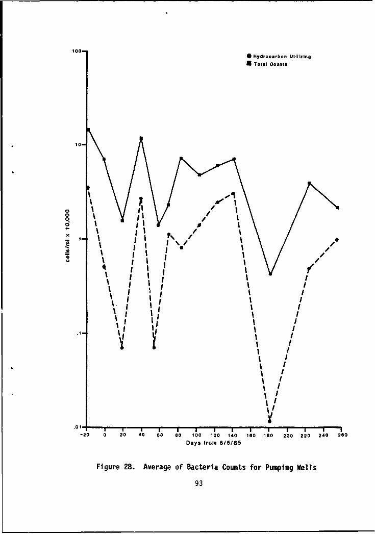
100,,
* Hydrocarbon Utilizing
* Total Counts
10
000,
0o I'/0Ro.. / l
I I \/S- I It I ISI! I -• ISI •I/
=I I I ISI I/
0r
S I 'I IxI
1.1 I I
I1I 1 II
.0 1 III
I
I\ II
-20 0 20 40 60 80 100 120 140 160 ISO 200 220 240 260
Figure 28. Average of Bacteria Counts for Pumping Wells
93

*HydroCarbon UtIlIzlig* Total Counts
10-
i4%
-20 0 20 40 60 so 100 120 140 180 100 200 220 240 260
Days from 6/5/86
Figure 29. Bacteria Counts for Soil
94

100-0* Hydrocarbon UtilIzIng
* Total Count*
10-
o-
.0 1
,- I ,
\ /
\/II
.0 ' I I II I I I I I I I I I-20 0 20 40 60 80 100 120 140 160 180 200 220 240 260
Days from 6/5/85
Figure 30. Bacteria Counts for Well M1
95

100,* H/drocarbon Utilizing* Total Counts
10-
xI
I\
II
I\
I
•0Io 0 I 4 / 1
69
I \1 \/-- ~I
" ~III
I 1 II I
II'///- I
I
,01 I ! I I '1'' I I II I I ' I -•-20 20 40 n 80 100 20 40 80 10 20 22 24 26
Oays rom /5/8
Figue 3. Bctera Cunt /:o Wel I
9'I

declining trend in pumping well microbe counts is observed while the in-
jection well microbe counts are considerably below background.
Finally, substantial microbe count changes for each plot are assumed
to occur where counts are outside the background range (counts for Days
-eO and 0, June 5, 1985). An increase in counts is observed in Well
M2 before Day 145 (October 27, 1985). No particular chemical or process
effect appears to correlate with this observation.
G. WELL PATTERN ORGANIC CONTAMINANT CHANGES
The initial state (before June 5, 1985) of the contaminants within
the well pattern area (soils and groundwater) is highly variable.
Concentrations of volatile organics in groundwater varied more than two
orders of magnitude in the wells within the treatment area. Total VOCs
in the pumping wells averaged 8.4 ppm before treatment. The key factors
associated with these data which affect the evaluation of changes during
treatment are discussed in this section.
Most of the mass of the organics per unit well pattern volume is in
the soil, in excess of 200 ppm for the soil versus less than 3 ppm for the
groundwater. Each unit volume of well pattern area, at 20 percent porosity,
will contain 10.4 times as much mass in the soil as in the groundwater at
the same ppm level. This is important for the following three reasons:
* Based on the addition of 299 pounds of hydrogen peroxide and a
usage of 3 parts of oxygen per part of contaminant, less than a
13 ppm change in the organic concentration in the soil could be
expected by peroxide activity. Since the varia ity of the
initial soil organic concentration exceeded this by orders of
magnitude, no change in total soil organic content was measured.
* If the principal source of the organics in the groundwater is the
soil, then it is not likely that any change in the groundwater
97

concentrations would be observed since the large soil reservoir
of mass would resupply the groundwater.
0 If considerable changes in soil or groundwater organic concentra-
tions are observed where most of the source is in the soil, then
the effect of the peroxide/nutrient mixture is to mobilize these
materials and transport them from one location to another. One
mechanism by which this may occur is through the formation of
biosurfactants, which have been observed to mobilize hydrocarbons
in enhanced oil recovery (Reference 22).
Total hydrocarbon and oil and grease concentrations in the soil are
listed in Table 13. Variations in both measurements over the initial 200
ppm levels indicate both considerable localized increase and reduction in
total hydrocarbon and increases in oil and grease. Since these changes
exceed the level of chemical reactivity of the hydrogen peroxide, the
peroxide/nutrient addition to the groundwater may have resulted in mobili-
zation of and redeposition of these materials within the well pattern
indirectly by formation of an intermediate chemical such as a surfactant
(Reference 22).
Total hydrocarbons concentrations in the groundwater are listed in
Table 14. Although variations between sampling points are large, a
comparison of samples collected August 8, 1985 and September 12, 1985
with those collected December 5, 1985 and February 17, 1986 indicates a
qualitative reduction in the groundwater organic level.
Table 15 lists groundwater oil and grease concentrations before and
during treatment. No considerable change with treatment is observed.
Table 16 lists well pattern groundwater concentrations of volatile
priority pollutants prior to and at three sampling times during treatment.
The major observations are summarized below.
98

TABLE 13. CONCENTRATIONS OF TOTAL HYDROCARBONS AND OIL AND GREASE IN SOIL
Hydrocarbon Concentrat ion (ppm) in Soil
Samples Taken Above 25' BGS Samples Taken Below 25' BGSDate Day - I
GC-FID O&G GC-FID O&G
Back-6/84 ground 221{ ....
- , Back-
4/85 ground 180-535 --- 140-195
8/85 69 ...... ND (0.05)-0.071 ---
12/85 188 ND (50)-1000 ND (200)-1300 ND (50) 800
Treatment began June 1985BGS - Below ground surface
99

TABLE 14. TOTAL HYDROCARBONS IN GROUNDWATER, GC SCAN (ppm)
Sample ID 8/8/85 9/12/85 12/5/85 2/17/186
PI ND (0.05) - ND (0.05) ND (0.05)P2 ND (0.05) ND (0.05)P3 - -P4 6.80 49.0 ND (0.05) 0.36P5 - - 0.31P6 ND (0.05) - NO (0.05) 0.076P7 - - ND (0.05) -P8 ND (0.05) 280.0 ND (0.05) 0.20P9 0.580 ND (0.05) ND (0.05) 0.37
11 0.150 ND (0.05) -
12 - - ND (0.05)13 1.40 1.70 ND (0.05) ND (0.05)14 730.0 ND (0.05) ND (0.05) ND (0.05)
M1 - ND (0.05)M2 4700.0 18.0 ND (0.05) ND (2.4)CC - ND (0.05) ND (0.05) 3.8
Blank 15.0 ND (0.05) 0.055Bailer Wash ND (0.05) ND (0.05) 0.061
Well was not sampledND(#) - Not Detected (detection limit)
100

TABLE 15. OIL AND GREASE IN GROUNDWATER (ppm)
Sample ID 5/23/85* 12/5/85 1/16/86 2/17/86
PI I <1 <1 2P2 2 2 2 <1P3 <1 <1 2 ND(1)P4 2 2 <1 <1P5 <1 <1 2 ND(1)P6 2 <1 1 1P7 <1 4 <1 2P8 1 2 2 ND(1)P9 1 2 <1 <1
II <1 I <1 ND(1)12 <1 4 <1 <113 1 <1 <1 <114 3 <1 <1 <1
Mi <1 2 2 1M2 3 <1 <1 <1CC - 4 1 <I
Blank I ND(1) ND(1)Bailer Wash 2 ND(1) ND(O.O01)
* Different Laboratory- Well was not sampledND(#) - Not Detected (detection limit)
101

TABLE 16. SUMMARY OF GROUNDWATER TCE, PCE, AND TRANS-I,2-DCECHANGES DURING TREATMENT
Priority Average AllPollutant Date Production 14 M2 CC
Wells (ppm) .
TCE 05/23/85 2.3 No Data No Data No Data(BeforeTreatment)08/08/85 1.7 No Data No Data No Data
(Decrease) 12/05/85 0.69 0.21 5.5 0.09902/17/86 0.47 .009 7.1 9.4
PCE 05/23/85 1.7 No Data No Data No Data(BeforeTreatment)
(Decrease) 08/08/85 1.8 No Data No Data No Data12/05/85 0.74 0.21 1.0 0.1102/17/86 0.46 0.023 10 0.10
Trans-1,2 DCE 05/23/85 0.027 No Data No Data No Data(BeforeTreatment)
(Increase) 08/08/85 2.4 No Data No Data No Data12/05/85 0.76 0.4 1.0 .00902/17/86 1.4 0.026 2.0 2.9
Vinyl Chloride 05/23/85 0.26 No Data No Data No Data(No Change) (Before
Treatment)08/08/85 0.32 No Data No Data No Data12/05/85 0.11 No Data ND (1.0) ND (.001)02/17/86 0.23 No Data 0.14 0.61
Chlorobenzene 05/23/85 0.021 No Data No Data No Data(Initial Rise (BeforeNo Net Increase) Treatment)
08/08/85 0.049 No Data No Data No Data12/05/85 0.095 No Data 1.0 .00102/17/86 0.029 No Data .1 0.1
Methylene Chloride 05/23/85 <0.005 No Data No Data No Data(Increase) (Before
Treatment)0n8/C/85 0.026 No Data No Data No Data12/05/85 0.30 0.059 ND 1 Q, kin tn.o01)
__02/17/86 0.12 ND (0.015) 27.0 1 2.8
No Data - Sample not analyzed "or this parameterND (#) - Not Detected (detection limit)< - detected at a value less than that shown
102

* PCE and TCE, the two compounds with initial concentrations in
excess of 1.5 ppm, show a reduction in concentration during
treatment. Both of these chemicals showed anaerobic reduction
during the treatability studies. Since hydrogen peroxide break-
through did not occur, except to a minimal level at the end of
treatment, a considerable portion of the well pattern may have
been in an anaerobic state during nutrient addition. The possi-
bility of chemical oxidation should also be considered for the
long residence times associated with this operation.
* Trans-1,2-DCE and methylene chloride concentrations showed a net
increase.
* Vinyl chloride and chlorobenzene concentrations did not show a
net increase.
Table 17 lists well pattern soil concentrations of volatile priority
pollutants prior to and at three sampling times during treatment. Major
observations are summarized below.
* Essentially only small quantities of PCE and TCE are measured in the
soil in comparison to the groundwater levels.
a The methylene chloride levels in the soil for August 1985 and
December 1985 (0.055 ppm and 0.23 ppm), although comparable in
concentration to the groundwater concentrations (<0.026 ppm and
0.30 ppm), are 10.4 times higher per unit volume of well pattern
in the soil than the groundwater (Table 15).
It appears that a higher activity of volatile priority pollutants occurr-
ed on the downgradient side of the well pattern area. This is illustrated
by the data in Table 18 and indicates that pollutants are either being
transported and concentrated downgradient or that higher initial concen-
trations existed downgradient, as evidenced by the 5 to 1 variation in
initial values between the average concentration of all pumping wells
(4.6 ppm) and the concentration in Monitoring Well CC (23.9 ppm).
103

CL
0)
CD C4 CD
0 v 0 0
V0)
V))
C))
- -4
0) -4
ILLJ cm in) a 0C~C) C 00
o) 0 V0L-) 0
F- <LU
C-,
>-
W-CCom U ) C
0m CL. CDCCDC
CL v CDLA- <
cc co 0 0.-j (o
co 0 0l 0-
VV)
c 0
0l CI- - = c o *-
E a)*
m 4- - 0
04- N -O
0 ) L- E- LL-- 4- aNL U)ý
2 104

TABLE 18. TOTAL CONCENTRATION OF VOLATILE PRIORITY POLLUTANTSIN GROUNDWATER (ppm)
DOWNGRADIENT
Date P Average P8 P9 M2 CC
05/23/85 4.6 8.0 8.9 No Data 23.9 (6/84 data)
08/08/85 6.2 3.9 6.2 No Data No Data
12/05/85 2.7 1.4 9.7 13.1 0.22
02/17/86 2.8 5.3 5.0 46.5 29.9
105

H. MECHANICAL AND ELECTRICAL EQUIPMENT
The various equipment and materials used in the demonstration system
were selected to provide durability and performance without interfering
with experimental results. Throughout the course of the demonstration,there were very few equipment or material-related problems. The few
problems that did occur were minor.
Once the pumps were installed, they all operated throughout the life
of the project without any mechanical problems. The pumps used did pre-
sent a potential problem due to excessive heat generation caused by the
extremely low pumping rates. Efforts to locate a pump that would operateat such low rates and still be durable enough to run continuously were
unsuccessful. For future systems, it would be beneficial to order custom-made pumps to meet the necessary specifications. The pump casings
were made of stainless steel which did not present a contamination or
reaction problem. Upon completion of the demonstration, some rust was
discovered but was not sufficient to have hampered system performance.
Electrical controls used to control pump operation performed as
designed throughout the life of the project. The discharge dnd re-circulation piping and pump electrical wiring present in the pumping
wells often made it difficult to use water level probes and precluded the
use of a bailer for removal of samples or a probe-type monitoring device
for collecting pH, dissolved oxygen, temperature and conductivity data.
The PVC and plastic materials used in all piping, joints, and valves
proved adequate. All piping and heat-welded joints performed well under
normal system operation. Several joir.ts cracked in a single occurrence
when valves were improperly adjusted, resulting in increased back pressureon the pumps. The PVC pipe installed near joints which had been welded
tended to become more brittle and were subject to cracking when subjected
to severe stress. The clear sections of PVC pipe placed in the system tomonitor flow from the pumping wells were more brittle than the normal
106

Schedule 80 PVC used in most of the system. The PVC pipe located
aboveground and exposed to a great deal of sunlight faded slightly and
also became more brittle. No failure was recorded due to this occurrence
and it was not believed to present a major problem. The PVC ball valves
used throughout the system were extremely functional but did not deliver
the degree of accuracy anticipated and had to be adjusted regularly.
With higher flows, this may not have been a problem.
The metering pumps used to introduce nutrients and peroxide were
very effective and allowed close control over the low volumes of in-
jected solution. The electrical timers installed later in the demon-
stration period allowed for effective operation of the system over-
night. Float valves installed on the injection wells were not effec-
tive in preventing overflow due to the very small infiltration rates.
The valves did not provide a complete seal and allcwed a small flow to
continue into the well. This flow was sufficient to continue to flood
the well. A valve providing a better seal, however, would have prevented
the problem of well flooding.
I. MITIGATION RESPONSE
Throughout the operation of the system, Well CC was monitored closely
for variations from historical concentrations of contaminants. In two
instances, some concern was given to elevated levels of contaminants in Well
CC. In the December 5, 1985 sampling round, the concentration for chromium
was considerably higher (3.3 ppm) in Well CC than in the other wells
sampled. A historical search showed similarly high levels for chromium
in Well CC. Analyses were repeated to verify the result. The value for
the second analysis was much higher (14 ppm) and cast some doubt on the
validity of either number. A letter of explanation was requested from
the laboratory which detailed several possible explanations for the wide
variance of values. The second instance of concern involved the relatively
high level ot total inorganic carbon in Well CC in the December 5, 1985
sampling round. Unfortunately, no earlier data are available because
107

total inorganic carbon testing had not been performed. In both cases,
evidence was insufficient to show that these levels of contaminants were
a result of system operation; therefore, mitigative response was not
recommended. Later sampling did not show concentrations as high.
The monitoring wells were used to monitor any changes that may have
occurred outside the treatment area that could be attributed to the
treatment operations. However, these wells were located within the
contaminated zone and should not have been expected to have lower levelsof contamination than wells located within the treatment area. Because
of the peninsula shape of the site, it was not possible to locate monitoringwells beyond the contaminated area. Leon Creek and surrounding land were
not Air Force property.
J. SAMPLING AND ANALYSIS
The Groundwater Monitoring Schedule followed at Kelly AFB is shown in
Table 2. In general, as implemented, sampling and analysis at Kelly AFBprovided useful results. The test kits proved to be economical and
accurate enough to monitor system performance. The use of test kits
allowed for quick results which could be implemented in adjusting system
operations if necessary. The test kits, however, are subject to humanerror and interpretation. Different operators performed the tests during
the span of the field program and, as a result, some procedures andinterpretations of results were not uniform. Also the test kits are
subject to interference by other chemical compounds in the groundwater.
It was possible that the high CO2 levels shown in using the test
kits could have been the result of other ions. A number of tests wereconducted to ensure that the reported CO2 values were the result of CO2
gas. In the first test, one sample of Well P9 water was analyzed over a
3 day periud, leaving the sample exposed to the atmosphere. Over the
3 day period, the measured C02 levels declined to a nondetect-
108

able level, indicating that CO2 was being released to the atmosphere.
The results of this experiment are given below as follows:
Date ppm COp By Field Kit Analysis
01/30/86 185
01/31/86 42
02/01/86 ND
In the second test, samples of fluid from the distribution box were
analyzed for CO2 before and after H2 02 addition. No difference in the
CO2 levels was observed, both were 59 ppm. Prior data indicated that injec-
tion solution CO2 levels were two to three times lower than the produced
fluid levels. This test demonstrated that peroxide addition did not
affect the CO2 level and that the most likely explanation for the reduction
of CO2 levels between produced and injected solutions was the exposure of
these solutions to the atmosphere.
A third series of tests was performed on P9 produced water to further
demonstrate that CO2 was the chemical species being measured by the field
test kit analysis. Two groups of samples of P9 water were monitored for
CO2 over a three day period (see results given below). In both cases,
duplicate samples were used. Samples 1 and 2 were left exposed to air
and demonstrate continual decline in CO2 levels. Samples 3 and 4 were
sealed in a bottle and not exposed to the atmosphere until the analyses
were performed. Samples taken and sealed on February 7 and analyzed on
February 8 and February 9 showed no decline in reported CO2 . Results are
as follows:
Exposed to Atmosphere Sealed Samples
Date Sample #1 Sample #2 Sample #3 Sample #4
02/107/86 144 ppm 143 ppm 150 ppm 151 ppm
02/08/86 40 ppm 36 ppm 160 ppm 156 ppm
02/09/86 5 ppm 6 ppm 150 ppm 158 ppm
109

These tests indicated that CO2 levels measured by field test kit
analysis reflect the presence of dissolved CO2 in the groundwater.
However, the source of the CO2 remains to be identified as biodegrada-
tion or shifts in carbonate equilibrium.
The laboratory analyses performed provided sufficient data on the
parameters of concern at the site. Because of the high cost of these
analyses only selected wells were sampled. Therefore, the data generated
did not always provide a complete overview of results due to the highly
variable nature of the site. This situation is discussed at length in
Section VI. One major inconsistency in the laboratory results is the
reporting of total hydrocarbons. The firs'st samples were sent to Aqualab
Inc., in Austin, Texas which reported oil and grease as total hydrocarbons.
Subsequent samples were sent to ERG in Ann Arbor, Michigan which reported
total hydrocarbons using a GC scan. These two numbers cannot be correlated
because the GC hydrocarbon scan quantifies lower molecular weight hydro-
carbons which will volatilize during the oil and grease extraction pro-
cedures. Although later samples were collected for both GC total hydro-
carbons and oil and grease, the lack of baseline data severely limits
conclusions that can be made about degradation of these compounds.
Future in situ field projects should consider more frequent hydro-
carbon analyses to monitor changes in organic levels and biodegradation
results. Onsite GC equipment could be rented and analyses performed
weekly or monthly depending on the size of the field project.
K. HEALTH AND SAFETY
The Health and Safety Plan developed for the field operations at
Kelly AFB was detailed enough to provide guidelines for safe practices
during all site activities. These procedures were strictly followed
by all field personnel. As a result, there were no field accidents
reported during the extent of field operations.
110
Adherence to health and safety procedures did not hinder effective
site operation in any way. Visitors to the site and any subcontractor
personnel were required to take necessary precautions detailed in the
Health and Safety Plan. Upon leaving the site at the conclusion of the
field activities, SAIC personnel were careful to ensure that all po-
tential hazards were removed.
111

SECTION V
PROJECT QA/QC
A. QA/QC PLAN
A detailed Quality Assurance/Quality Control Plan was developed by
SAIC and approved by the funding agencies for all aspects of the demon-stration at Kelly AFB. The major points of this plan as performed at
Kelly AFB are summarized in this section.
B. SAMPLING PROCEDURES
Bailer decontamination was performed before sampling each well.
This decontamination procedure involved scrubbing the bailer withAlconox® detergent followed by complete rinsing with distilled water.
The drawstring was replaced between sampling of each well and sterile
gloves were worn by sampling personnel at all times. Before sample
collection, each well was purged of up to five times its saturated zone
volume. Field blanks and bailer washes were taken as necessary.
All equipment used in soil sample collection was steam-cleanedprior to contact with the subsurface. Sterile gloves and containers
were used and gloves were replaced between each sample.
Accurate records were maintained throughout the sampling procedure
to document the sampling environment, sample characteristics, and otherpertinent information. Each sample was identified by a label showing
its specific characteristics. Samples being sent to laboratories were
shipped immediately by overnight courier in coolers with sufficient
blue ice to maintain a temperature of approximately 4VC during ship-ment. All samples were sent to approved laboratory facilities and
112

were accompanied by chain-of-custody documents to ensure accuracy of
reporting.
C. TESTING PROCEDURES
Onsite testing was performed by both meters and chemical test kits.
The accuracy of these procedures was assessed regularly, using a number
of methods. All meters were calibrated weekly using standard solutions.
Spare meters were also used to verify these readings on a regular basis.
Selected test kit results were checked by analyzing standard solutions
provided by a local analytical laboratory. These checks showed test
kit results to be within at least 20 percent of standard solution values.
Upon collection of groundwater samples, readings were taken immediate-
ly for dissolved oxygen, pH, temperature, and conductivity. The remain-
ing sample was placed on ice until analytical laboratory analysis were per-
formed. EPA standard laboratory methods were used, as discussed in Section
III.B. At least one replicate, field blank, and bailer wash were analyzed
for each round of sampling.
D. SYSTEM AND PERFORMANCE AUDITS
A complete audit was performed in November 1985. This audit re-
viewed both field and office operations. The following items were
addressed:
* Data recording practices
* Test kit analysis schedule
9 Data analysis techniques
e Quality control
e Data management
* Reporting audits
* Data validation
113

e Sampling techniques
* Field meter performance.
E. PREVENTIVE MAINTENANCE AND ENGINEERING QUALITY CONTROL
The field operators performed regular assessments of system opera-
tion which included the following items:
0 Inspection of all welds and joints for leaks
* Inspection of all wiring for proper connections, exposed or
worn wiring, and possible overloading of circuits
0 Inspection of pumps for proper operation
0 Inspection of pump controls for proper operation
* Regular calibration of all valves to provide accurate measure-
ment of flow
e Regular maintenance and calibration of all meters and measure-
ment instruments.
All technical work performed on this project was subject to SAIC's
peer review process. A peer review committee consisting of senior level
employees from a variety of disciplines worked closely with the QA officer
to review engineering performance. These activities helped to ensure the
highest level of engineering quality in all aspects of the project.
114

SECTION VI
IMPLEMENTATION AND COST OF IN SITU TREATMENT
A. GENERAL CONSIDERATIONS FOR IMPLEMENTING IN SITU BIODEGRADATION
This section describes the activities involved in the design and
operation of an in situ treatment system using the same general ap-
proach as in the Kelly AFB demonstration. The reader should be aware
that other methods of groundwater circulation and treatment are also
available. These methods include infiltration trenches or troughs and
conventional land farming techniques. This generic plan will discuss
only groundwater pumping and injection via wells.
1. Site Characterization
Characterizing a hazardous waste site is one of the most com-
plex activities in any remedial action. The site characterization
requirements for in situ treatment are even more extensive than for most
other remedial alternatives. Figure 32 outlines the site characteriza-tion process associated with in situ treatment, presents the associated
tasks, and lists the data that can be expected from these tasks. All ormost of this data will be necessary before an in situ treatment system
can be designed. Activities associated with the generally prescribed ap-
proach for characterizing DOD or CERCLA sites are identified on Figure 32
above the dotted line. The activities more specific to in situ treatmentare listed below the dotted line. Major differences from those activities
normally performed during a remedial investigation are groundwater and
soil treatability studies. The next section discusses the types of treat-
ability studies that may be performed and when they would be appropriate.
115

(A
4-) CA
4) V ) *.
vi 4) LA9
cc- 0 _ Q 06 0 4) 1 430 -9-. 1 41 >%0 u S- 06 in
0.J 4) f 0) 4J 9)
tf . -C. 4-)1- 0 I J( 4)~ 4.*- ~ u 4- 04 .C E
0Lv- 4) U S Wn0 0 J.i U0 0 CE 0 1n S- -
EU0.C - 0. 00 * 4-) 0100 0-i "E4 U 9 E
a) 09 W. 0 m -0 4J in) .0-
U'0 4) .- - a)J. inA 9 -i 00. U
Lmj -04-) 41 4)~f 4 V) 0 0- =01 -3
4). o 04t I . - a- 0 cS- co S- 4- in. 4-)E
4-0 - 00 0. 0 CU ~ 9,:; 0) IV 4-00 06- XmfC X 4- CLS 0.04- 0
o V04 tu T;4 00 cm .- r- 4.9
c)-u =- d-)1 C n1 a) 4-. a) 4) S-( sm-0)3 -V c z -0 0)41 9 *.-EU E-1-*v)
0 m U d 0. L. 04 0 in L9 V).c 194.>I 0>a W S- M 0 >,.OE i~- 0
V) ) -0 0 4-.j 3.0 co9 9j CD =.1- :co 0.0(-) U-
00.0 000C oes49. 00 0-4)00 0 S
0l4-.
fn 0IA 9
9 4.
E~ia) 00.14jC tm to
-&- - W L a) (v - a4-)
0 v . u0
0) 5- V) U0 9 4.)to
.4.9 9.~ 007 4) 9
9~ U- 000 1- S0. 4 0.)
CO~4 06)> (Po 01 0U 1-0-00) 0 uV 4- 4-U (
- 3n 9 .0 . u0- --.-. *C'-ma- oU ) 4-4)c
(A m7 =7( J 4 - 4) - -
0 ')=to c -- 1 54- = Q 10O-- 1)n0 cin 50 m 4) L 4.) V 1-0 C1-
LI.xr
4-J ZILL. 0LJ. 0I- Cl IA =A - V AL)~V -In 0-I >.~a~ LA-
9rz U=- LA
116

2. Soil and Groundwater Treatability Studies
Treatability studies are normally conducted following site
characterization and contaminant assessment and include chemical and
microbiological studies of both soil and groundwater from a waste site.
Treatability studies for in situ treatment are designed to provide ad-
ditional data on waste characteristics and the biodegradability of the
contaminants present, identify and quantify the microbial population
present in the subsurface, and evaluate potential chemical effects of
in situ treatment on soil and groundwater characteristics. The studies
are conducted with soil and groundwater from the waste site and are
designed to reflect various aspects of the proposed treatment approach.
a. Contaminant Biodegradation Studies
Biodegradation studies are conducted with soil and ground-
water from the site and provide information concerning waste charac-
teristics including the biodegradability of the contaminants. Informa-
tion can also be obtained from these studies to determine if toxicintermediate metabolites or oxidation/reduction products will be formed
that may interfere with in situ treatment success.
Biodegradation studies can range from sophisticated micro-
cosm studies to simple microbial plate counts, depending on the type ofinformation required from the study. Full-scale microcosm studies are
useful when the groundwater and soil contain a wide variety of organic
and inorganic contaminants and the chemical interactions between the
soil and groundwater and the treatment solutions are uncertain. Micro-cosm studies may also be warranted when the contaminated soil and ground-
water have not been fully characterized with respect to contaminants
present, or when sufficient information is unavailable on the treata-
bility of particular contaminants. These studies are useful in deter-mining whether nutrient addition is warranted and, if so, what formula-
tion would be best suited to the microbial populations present. Full-
117

scale microcosm studies may not be necessary when only a few contaminants
are present in the soils and groundwater or when existing data supports
the biodegradability of particular compounds of concern.
Simpler biodegradation studies can be conducted by per-
forming microbial spread plate counts using the contaminated ground-
water as the sole carbon source for aerobic bacteria. Incubation of the
plates is followed by cell counts to determine if the subsurface micro-
bial populations are able to use the contaminants. These studies pro-
vide only general but often useful information regarding potential
treatability of the contaminated soil and groundwater.
Contaminant biodegradation studies can be designed to
evaluate both aerobic and anaerobic treatment approaches. Both oxygen
and hydrogen peroxide treatment can be evaluated in aerobic microcosms.
In addition, various nutrient formulations can be tested to determine
the necessity and/or type of nutrients for biodegradation. Microcosm
studies conducted over extended periods of time can provide data on
biodegradation rates which, when combined with specific site charac-
teristics such as hydraulic conductivity and soil permeabilities, are
important to determining the feasibility of in situ biological treat-
ment. The treatability program can be quite diverse but should be
designed to help refine the proposed treatment approach.
b. Microbiological Investigations
The design of microbiological investigations can be quite
varied and also depends on existing microbial data available on the
site and the type of additional information required. Typically,
microbial studies consist of direct and/or viable cell counts performed
using dilution-spread plate procedures. These studies are relatively
inexpensive to perform and are useful for determining if an adequate
microbial population exists for conducting in situ biological treatment
of the contaminants present. In addition, data on the types of microbes
118

present and their distribution can be obtained. Microbiological studies
can also provide information regarding general biodegradability of the
contaminants, as discussed above with regard to treatability studies.
c. Soil Tests
Soil column tests are also conducted with soil and ground-
water collected from the site. These studies are important for evalu-
ating soil perneability and the chemical reactions which may occur
between the soil and groundwater and the proposed in situ treatment
solutions (oxygen source and nutrients, if necessary).
Soil column studies are usually conducted with permeameters;
groundwater and treatment solutions are passed through the soil, and
leachate solutions are collected and analyzed. Various treatment solu-
tions can be permeated through several permeameters to optimize treat-
ment solutions with respect to soil and groundwater chemical effects.
Mineralogical and petrological studies may also be performed to gain
a greater knowledge of physical and chemical properties of soils.
Results can be obtained from these studies which will accu-
rately reflect problems and conditions which may arise during field
implementation. These data include breakthrough curves of treatment
solution constituents, information on exchange reactions between the
soils and treatment solutions, and the effects of treatment solutions
on soil permeability. Each of these factors are important to in situtreatment success and should be considered before final system design
and implementation.
3. Design of the Well and Chemical Systems
The design of a pumping and injection treatment system requires
a great deal of site-specific information. These information needs
were presented as "Data Generated" on Figure 32. This section discusses
119

how the data can be used in making design decisions and describes some
alternatives available in designing an in situ system using pumping and
injection wells.
a. Well Design
The size, number, and spacing of pumping and injection wells
will depend largely on site-specific characteristics. The spacing of
wells will be largely dependent on the permeability of soils and pumping
rates. Wells in less permeable soils will generally need to be closer
together in order to effect treatment in a reasonable period of time.
The size of the well will also be affected by soil permeabilities as
larger diameter wells will allow for higher rates of pumping and injec-
tion. The ratio of pumping to injection wells should be maintained so
that no excess groundwater is generated. The cost of removing large
amounts of hazardous wastewater would greatly negate the cost-efficiency
of in situ treatment. The spacing of wells can be varied over a site
to compensate for subsurface variabilities.
In sizing of wells, attention should be paid to the amount
of space that will be needed for the pump, piping, and electrical equip-
ment such as water level sensors. In addition, enough room should re-
main for the use of a bailer and monitoring devices.
b. Transport and Mixing System
Many options are available for the mixing of nutrients and
peroxide with the groundwater. The most desirable is an in-line system
whereby nutrients and peroxide are added directly into the transport
lines between pumping and injection wells. This system, however, is
only practical at sites with very high pumping and injection capacities.
In such cases, flow regulation into injection wells is unnecessary and
overflow of the wells is not a problem. At low flow rates, it is
necessary to monitor pumping and injection volumes very closely. It
120
then becomes more difficult to continuously monitor flow rates and
chemical concentrations to ensure that too much flow or too high a
chemical concentration is not entering the injection wells.
For low flow rates, a batch-type mixing system will pro-
bably be most feasible. A large central mixing tank will allow
nutrients and peroxide to be added to desired concentrations before
being transported to the injection wells at regulated flows. Tanks
should be protected against overflow and provide a sampling point to
analyze circulating groundwater.
The size and location of a central mixing system will de-
pend largely on the flow rate, size of the site, and site topography.
For large sites, more than one mixing system may be necessary. Gravity
is generally the best method of groundwater transport. The pumps in
the pumping wells may provide enough pressure to transport water to
the central mixing tank in cases where the topography prohibits gravity
flow. Also, the head on the mixing or distribution tank may provide
sufficient pressure to transport water to the injection wells.
c. Treatment Chemicals
Selection of nutrient and oxygen sources will be important
to system design. Precipitation was a major problem at the Kelly AFB
demonstration site. It is important to quantify this problem prior to
system operation and take measures to prevent it from adversely affect-
ing the system. It may be necessary to weigh the advantages of adding
nutrients against the potential for precipitation. Enhanced biodegrada-
tion may be possible at some sites without the addition of nutrients.
Hydrogen peroxide proved to be an effective supplier of
oxygen and requires little special equipment. Other methods of oxy-
genation such as forced air do require additional mechanical equip-
ment which require additional maintenance.
121

d. Equipment and Material Selection
Durability is the primary factor to consider in selecting
materials and equipment to use in an in situ treatment system. The
system will be operating continuously and place a great deal of stress
on pumps and piping. System downtime will cause delayed treatment
and added expense. It is also important that all materials be non-
reactive and noninterfering. This requires complete knowledge of how
all materials will react with the contaminants onsite and proposed
treatment chemicals. If this is unknown, simple laboratory scale
studies can be performed.
Pumps and electrical controls will be subject to the most
stress. All metal surfaces should be corrosion-free and pump housings
must be durable enough to prevent any leaking of oil. The pump itself
need not have a variable flow capacity as the flow can be controlled
by valves at the surface. The pump should be rated within the full
range of expected pumping rates to avoid unnecessary stress on the pump.
Valves and flow meters should be sensitive enough to accurately measure
the smallest flow anticipated for the well.
e. Operational Characteristics
The system will be operated continuously for a long time
and as high a degree of automation as feasible should be implemented.
Automatic devices in the pumping wells should turn off the pump when
the water level is too low. Similar devices should be incorporated
into the injection wells and mixing tanks to prevent overflow. Timers
can be incorporated to cycle pumps, if necessary. More complex systems
at very large sites could be designed to regulate flow and adjust
pumping rates automatically. Although this would be expensive, the
cost could probably be recovered in reduced operating expenses.
122

Another operational consideration is the provision for
sampling and monitoring, as these operations are integral to any in
situ treatment system. As mentioned in the Well Design Section, wells
should be designed large enough so that samples may be retrieved. In
addition, a great deal of onsite analysis may be performed to monitor
system performance. An onsite GC unit would allow for more frequent
sampling and more samples at a lower cost than an offsite laboratory.
It also provides results in a much more timely manner to allow for
operational monitoring. A facility suitable for this purpose will be
necessary, as well as an area for decontaminating field equipment and
disposing of laboratory wastes. Sampling soil is more difficult and
more expensive than sampling groundwater. Analyzing soils is also
more expensive. It is, therefore, probable that soils will be sampled
much less frequently and groundwater results will be relied upon to
provide information on performance of the system. The most logical
soil sampling schedule would be to do widespread sampling at the vary
beginning and end of treatment and very little, if any, during treatment.
4. Copstruction of the System
Construct ion will always begin with well installation and
wells need to be installed properly. A poorly developed well will be
of little use to the treatment system due to reduced pumping rates.
Fines left in pumping wells could cause pump damage and mud and silt at
the bottom of the well could cause pump clogging and cloud groundwater
samples. Pumps should not be placed in the wells until as much of this
material as possible is removed.
Pumps, piping, and electrical equipment placed in the wells
should be constructed so that removal can be performed easily without
disrupting the entire system. Glues should be avoided whenever pos-
sible to reduce the possibility of chemical interference. Welding,
threaded joints, or compression fittings can all be used w'ith good
results.
123

A central electrical circuit boa.rd with individual controls
for each pump should be located within close proximity to the site
for emergency shutdowns. The electrical lines should be buried
underground to prevent accidents and disruption of power.
5. Startup and Operation
Once construction is complete, groundwater should be circulated
for a few weeks without introduction of treatment chemicals. This should
provide sufficient time to adiust pumping and injection rates and remove
all residual fines from pumping wells. When pumping and injection rates
are known, it is then simple to calculate the desired nutrient and
peroxide concentrations. This iritial period also provides a shake-
down of the system so that any operational problems may be resolved be-
fore treatment is commenced.
The first few weeks of treatment should be monitored carefully
to determine system performance. Results of frequent onsite testing
will be useful irn determining chemical transport and guide decisions
as to the concentrations of treatment chemicals and/or the rates of
pumping and injection. Once the system is operating effectively, the
frequency of onsite sampling and analysis can be reduced to a reason-
able level to provide long-term performance analysis. Onsite analysis
is not expensive or difficult but it can be very time-consuming. Field
staffing should be scheduled according to the quantity of tests to be
performed. Normal oporation and maintenance of a treatment facility
should rarely require more than one individual, however, relevant health
and safety regulations require more than one person to be present during
activities at a hazardous waste site.
B. BREAKDOWN OF COSTS AT KELLY
The actual costs of performing the demonstration at Kelly AFB are
p~csnt~d in this section. The costs presented are approximate and
124
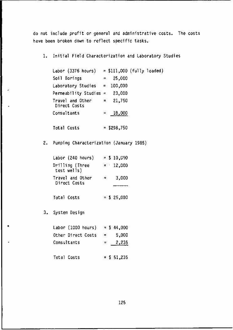
do not include profit or general and administrative costs. The costs
have been broken down to reflect specific tasks.
1. Initial Field Characterization and Laboratory Studies
Labor (3376 hours) = $111,000 (fully loaded)
Soil Borings = 25,000
Laboratory Studies = 100,000
Permeability Studies = 23,000
Travel and Other = 21,750Direct Costs
Consultants = 18,000
Total Costs $298,750
2. Pumping Characterization (January 1985)
Labor (240 hours) = $ 10,000Drilling (Three = 12,000test wells)
Travel and Other = 3,000Direct Costs
Total Costs = $ 25,000
3. System Design
Labor (1000 hours) = $ 44,000
Other Direct Costs = 5,000
Consultants = 2,235
Total Costs = $ 51,235
125

4. System Construction and Startup
Labor (800 hours) = $ 24,000
Travel and Expenses = 10,000
Drilling (13 Wells) = 33,000
Electrical - 4,000
Piping = 2,200
Pumps/Controls = 4,000
Tools/Misc. Supplies = 1,500
Total Costs = $ 78,700
5. System Operation, Sampling, and Analysis
Labor (2150 hours) = $ 55,000Travel and Expenses = 32,000
Onsite Trailer = 2,000Rental (10 months)
Onsite Assistanceand TreatmentChemicals = 36,000
Sampling and OnsiteAnalyses = 6,300
Maintenance = 550
Misc. Field Supplies = 1,725
Soil Sampling = 4,850
Health and Safety = 800Equi pment
Chemical Analyses = $ 50,000(56 groundwatersamples, 19 soilsampl es)
126

Biological Analyses 4,000
(30 groundwater
samples, 10 soil
samples)
Shipping = 3,350
Total Costs $196,575
6. Office and Administrative Costs
Labor (4670 hours) $150,000
Word Processing 1,600
Graphics and Xerox 4,500
Computer Use 1,000
Temporaries = 5,000
Phone 10,000
Total Costs = $171,100
Sum of all Costs $821,360
C. COST ESTIMATION FOR IN SITU BIODEGRADATION
Table 19 presents a list of variables that can be used in estimating
the cost of performing in situ treatment. Four worksheets are presented
in Figure 33 which provide a simple method of cost estimating using these
variables. The worksheets assume a continuous site of relative homogeneity
and uniform thickness of contamination. All costs are ultimately converted
to dollars per ton as an end result so that in situ costs can be compared
to costs of other alternatives such as removal. The cost categories
considered in the worksheets correspond to those activities discussed in
the generic site plan, specifically: site characterization, system design,
system construction, and system operation. Variables used on the work-
sheets are described in Table 19.
127

TABLE 19. DESCRIPTION OF VARIABLES USED
ON COST ESTIMATION WORKSHEETS
A area to be treated (acres)Ca total analytical cost per sample (includes metals, priority
pollutants, and total hydrocarbons)
Ccs concentration of contamination in soil (ppm)Ccw concentration of contamination in groundwater (ppm)
Cd cost of installing wells (per foot of well)C1 field operation labor costs (per employee per day)
Cn cost of nutrients (per ton)
Cp cost of peroxide (per ton)
D depth of wells (feet)Df fluid density (pounds per cubic foot)Ds soil particle density (pounds per cubic foot)
E fraction of all wells sampled during a single sampling eventH thickness of contaminated zone (feet)
L total number of laboratory sampling eventsM total mass of contaminated soil (tons)
Mp concentration of hydrogen peroxide at introduction to groundwaterN total number of wells
Na number of wells per acreNi number of injection wells
Np number of pumping wells
Npv number of pore volumes circulated during treatment
P porosity of soil (fraction)
PV pore volume of contaminated zone (gallons)
Q total circulation rate (gallons per day)
Qi flow into individual injection wells (gpd)S average number of field personnelSf frequency of laboratory sampling events (days between events)
Sp number of laboratory sampling events per PV displacement
Sw number of wells sampled per event
128

TABLE 19. DESCRIPTION OF VARIABLES USED
ON COST ESTIMATION WORKSHEETS (Continued)
t time for one pore volume displacement (days)
T total time required to achieve cleanup (days)
Un nutrient use per unit mass of contaminant (lb of nutrientper lb contaminant)
Up peroxide use per unit mass of contaminant (lb of peroxideper lb contaminant)
Utn total nutrient required (pounds)
Utp total peroxide required (pounds)
129

Worksheet 1. Site Characterization
(1) Records Search: #people x #days x rate = $
(2) Define Environmental Setting: #people x #days x rate = $
Assessment of site specific geology and waste characterization:
* Well drilling: #wells x #feet x cost per foot = $0 Field labor: #persons x #days x rate = $
0 Travel: (#days + 10) x #persons x air fare = $
e Expenses: (auto + per diem + daily expenses) x #persons x
#days = $
a Petrological and/or mineralogical assessments: #soil samples x
cost = $
a Metals Analyses: #wells x cost of analysis = $* Priority Poll. Analyses: #wells x cost of analysis = $e Hydrocarbons Analyses: #wells x cost of analysis : $e Microbes Analyses: #wells x cost of analysis = $e Analysis of Results: #people x #days x rate = $
e Other Direct Costs: estimate = $
(3) Total = $
Treatability Studies:s Permeability Testing: #tests x rate = $e Degradation Tests: #tests x rate = $
0 Analysis of Results: #people x #days x rate = $
e Other Direct Costs: estimate : $
(4) Total = $ 0
** Site Characterization Cost Per Ton = [(1) + (2) + (3) + (4)] * M :$ _ _
Figure 33. Cost Estimation Worksheets
130

Worksheet 2. Operating Characteristics
Site Characteristics
A = area of site = acres.
Ds= particle density =lb/ft 3 .Df = fluid density = lb/ft3.
P = porosity of soil =
H = thickness of contaminated zone = ft.
M = total mass of contaminated soil [A] [H] [Ds] [1-P] [21.78] = tons.
PV = pore volume = [A] [H] [P] [325,872] = gallons.
Ccs = concentration of contamination in soil = ppm.
Ccw = concentration of contamination in groundwater = ppm.
Design Parameters
Na = number of wells per acre =
N = number of wells = Na x A =
Np = number of pumping wells =
Ni = number of injection wells =
D = depth of wells =
Qi = flow per injection well = gpd.
Q = total circulation rate = Qi x Ni = gpd.
MP = concentration of peroxide = ppm.
SP = sampling events per pore volume displacement =
E = fraction of wells sampled per event =
Un = nutrient use per unit mass of contaminant = lb/lb.up = peroxide use per unit mass of contaminant = lb/lb.
Sw = number of wells sampled per event = NASpE =
Figure 33. Cost Estimation Worksheets (Continued)
131

Worksheet 2. Operating Characteristics (Continued)
Operation Parameters
T = time to achieve cleanup = 325,800 [Cc, Ds (1-P) + Ccw Df P] Up H A =
_ days. Q Mp Of
t = time for 1 PV displacement = PV/Q = days.
Npv = # pore volumes circulated during treatment = T/t =
Utp = total peroxide used* = Up[(Ccs)(M x 2000)(10-6) + (Ccw)(PV x Df)(10 6 )/
(7.48)] = lbs.Urn = total nutrient used = Un[(Ccs)(M x 2000)(10-6) + (Ccw)(PV x Df)(10 6 )/
(7.48)] = lbs.Sf = sampling frequency = t/sp = every days.
L = total # sampling events = T/Sf =
S = average # of field personnel N/40 =
Unit Cost Parameters
Cd = zost of drilling = $ per foot.
Cn = cost of nutrients = $ per ton.
C = cost of peroxide = $ per ton.
Ca = analytical costs = $ per sample.
Cl = (S) (daily rate + travel + expenses) $ per day.
CS = cost of system shutdown = $ per foot of well.
Note: The numbers generated here are used on Worksheets 3 and 4.*Utp assumes all contaminants are aerobically degradable.
Figure 33. Cost Estimation Worksheets (Continued)
132

Worksheet 3. Design and Construction Costs
Design Costs:
#people x #days x rate = $Other direct costs = $
(1) Total = $
(2) Well Installation: N x D x Cd = $
Field Labor:
(10 man days/well) x N x Cl $
Other Direct Costs: estimate = $
(3) Total = $
Construction Materials and Supplies:
* pumps: cost x Np = $
* piping: cost x total feet = $0 controls/electrical: cost x Np = $
e flow valves + meters: cost x Np= $
* mix tank: # x cost = $
* distribution tank: # x cost = $0 tools: estimate = $
* misc. supplies: estimate = $e chemical feed system: # x cost = $
(4) Total = $
** Construction Cost Per Ton = [(1) + (2) + (3) + (4)] + M =$ _ _
Figure 33. Cost Estimation Worksheets (Continued)
133

Worksheet 4. System Operation and Shutdown
Chemical Costs: Peroxide: Utp x Cp = $
Nutrients: Utn x Cn = $
(1) Total = $ -0
Laboratory Costs:Total Analytical Costs: L x Ca x Sw $
or:
Priority Pollutants: L x cost x Sw = $
Metals: L x cost x Sw = $
Hydrocarbons: L x cost x Sw = $Microbes: L x cost x Sw = $
(2) Total = $
Costs of System Operation:Field Operation, Sampling, and Analysis Labor: T x Cl = $
Other Direct Costs: estimate = $Maintenance: 5% of construction costs annually = $
(3) Total = $
On Site Analysis:GC Rental or Purchase: cost over life of project $
Weekly Test Kit Analyses: #tests x N x T/7 x cost = $
Sampling Supplies: estimate (small cost) = $(4) Total = $
System Shutdown:
(5) Cost of removal and grouting of wells = N x D x Cs = $
** Operating Cost Per Ton = [(1) + (2) + (3) + (4)]/M = $
Total Cost Per Ton = $
Figure 33. Cost Estimation Worksheets (Concluded)
134

Worksheet 1 calculates the costs of performing site characterization.
All of these costs are not specific to the performance of in situ treatment
and the required activities will vary from site to site. This worksheetwill provide the user with a method of developing a general overview of
potential costs of performing a site characterization.
Worksheets 2, 3, and 4 are directed specifically at the performance
of in situ treatment. Worksheet 2 is used for developing all variables
that will be used in calculating costs of treatment. This worksheet is
divided into four categories: (1) site characteristics, ,2) design
parameters, (3) operation parameters, and (4) unit cost parameters. The
site characteristics information will be generated as a result of site
characterization activities. Design parameters will be established by
using data gained through site characterization and treatability studies.
Operation parameters can then be calculated as shown. The unit costs of
the major treatment components are estimated and applied to the specific
operation parameters for the site. Using this information, design and
construction costs are calculated in Worksheet 3 and system operation andshutdown costs are calculated in Worksheet 4.
D. SENSITIVITY ANALYSIS FOR CONSTRUCTION AND OPERATING COSTS
Using the worksheets presented in Figure 33, a cost sensitivity
analysis was performed to determine how the cost of in situ treatment to other
treatment was affected by changing various parameters. This sensitivity
analysis is useful in comparing the cost of in situ treatment to othertechnologies. Sensitivity analyses of this type should be performed for
future applications of in situ treatment in order to develop the most
efficient design possible. The analysis only deals with construction and
operating costs. It is assumed that site characterization and design
costs will not fluctuate greatly between sites and are therefore not
considered. These costs are also not unique to in situ treatment andwould bias the total cost of treatment.
135

The sensitivity of cost for performing in situ will depend on design
parameters as well as site parameters. Design parameters are the variables
in the cost of treatment deper.-ent upon the design of the system. The
most important of these will be the spacing and number of wells installed.For the cost model, wells are considered by number per acre (N). The
relationship between spacing and number of wells per acre is as follows:
* 10 foot spacing ---- > 400 wells per acre
e 15 foot spacing ---- > 200 wells per acre
* 20 foot spacing ---- > 100 wells per acre
* 50 foot spacing ---- > 50 wells per acre.
Increasing the number of wells will increase the total circulation rateand reduces the time for treatment. This will act to reduce the duration
of operating costs, however, more wells also means increased construction
and unit operating costs. Increasing the number of wells may require the
number of sampling events per pore volume and the fraction of wells to besampled (E) to be decreased to a reasonable value. The circulation rate
may or may not be a design function. If transmissivity of soils is high,
some latitude may exist in determining the flows to be used. In many
cases, such as at Kelly AFB, soil conditions will be the major factor in
determining flows. Other design variables of importance include the
concentration of hydrogen peroxide (Mp), the well depth (D), and analytical
and labor costs (Ca, Cl). However, there is much less control over thesefactors. Peroxide concentrations will be chosen to be the highest feasible
values at the given site. The depth of wells will be largely determined
by site conditions. Analytical and labor costs can be minimized through
efficient operation but will still be determined greatly by the size of
the site.
Site variables are those cost variables solely dependant on site
specific conditions. These include both rate and mass variables. Ratevariables include soil permeability which determines flow (Q) and nutrient
and peroxide use (Un and Up). The value assumed for Un may be an upper limit
136

for nutrient use and was based on initial recommendations from Aquifer
Remediation Systems for the Kelly AFB site. Although this value may be
an upper limit, the cost of nutrients has a small impact on the econimic
evaluation of in situ treatment. Mass variables include contaminant
concentrations (Ccs and Ccw), densities (Ds and Df), porosity (P), and
the extent of contamination (H and A). The most important of these
variables will be the flow potential and the extent of contamination.
The cost sensitivity analysis presented in this section is an attempt
at showing the relationships between the variables involved in in situ
treatment and their relative importance. It does not necessarily present
realistic costs of performing in situ treatment at a particular site and it
does not represent the costs and site conditions experienced at Kelly
AFB.
The analysis was performed by first developing a baseline site
situation. This baseline situation is presented as a completed "Worksheet
2" and presented in Figure 34. Ten scenarios were then developed by
adjusting the values for number of wells (N), flow (Qi), area (A), thickness
of contaminated zone (H), well depth (D), contamindnt concentrations (Ccw
and Ccs), analytical costs (Ca), peroxide use (UP), and field labor
required (S). The costs of these ten scenarios and the cost of the baseline
situation are presented in Table 20.
This analysis provides a number of observations regarding the cost of
performing in situ treatment. The affect of each variable change presented
* in Table 20 is discussed in the following paragraphs.
Scenario #1. Reducing the number of wells by half saves a great
deal of money by reducing the construction and shutdown costs. Though
the time for treatment is doubled, laboratory costs went down due to fewer
wells to sample. This would probably be offset somewhat by increasing
the percentage of wells sampled when spaced further apart. Labor costs
went up, but were partially offset by the need for fewer personnel and
smaller maintenance costs.
137

Worksheet 2. Operating Characteristics
Site Characteristics
A : area of site = 1 acre.
Ds particle density = 170 lb/ft3.
Df= fluid density = 62 lb/ft3.P = porosity of soil 0.2H = thickness of contaminated zone 1 10 ft.
M = total mass of contaminated soil = [A] [H] CDs] [1-P] [21.78] = 29,621 tons.
PV = pore volume = [A] [H] [P] [325,872] = 651,744 gallons.Ccs = concentration of contamination in soil = 100 ppm.
Ccw = concentration of contamination in groundwater = 10 ppm.
Design Parameters
Na = number of wells per acre 200
N = number of wells = Na x A = 200
Np = number of pumping wells = J50
Ni = number of injection wells 50
D = depth of wells = 30 .
Qi = flow per injection well = 250 gpd.
Q = total circulation rate = Qi x Ni = 12,500 gpd.
Mp = concentration of peroxide = 500 ppm.
Sp = sampling events per pore volume displacement = 1
E = fraction of wells sampled per event = 0.5
Un = nutrient use per unit mass of contaminant = 5 lb/lb.*up = peroxide use per unit mass of contaminant = 5 lb/lb.
Sw = number of wells sampled per event = NASpE 1 100
*Upper limits for nutrient use based on initial rpcommendation for
Kelly AFB site.
Figure 34. Characteristics of Baseline Scenario for
Cost Sensitivity Analysis
138

Worksheet 2. Operating Characteristics (Continued)
Operation Parameters
T = time to achieve cleanup = 325,800 [Crs Ds (1-P) + Crw Df P] Up H A =
Q M p Df
577 days.
t = time for 1 PV displacement = PV/Q = 52 days.
Npv = # pore volumes circulated during treatment T/t = 11
Utp = total peroxide used* = Up[(Ccs)(M x 2000)(10-6) + (Ccw)(PV x Df)(10-6)/
(7.48)] = 29,891 lbs.
Utn = total nutrient used = Un[(Ccs)(M x 2000)(10-6) + (Ccw)(PV x Df)(10- 6 )/
(7.48)] = 29,891 lbs.
Sf = sampling frequency = t/sp = every 52 days.
L = total # sampling events = T/Sf = 11
S = average # of field personnel = N/40 = 5
Unit Cost Parameters
Cd = cost of drilling = $ 100 per foot.
Cn = cost of nutrients = $ 1000 per ton.
Cp - cost of peroxide = $ 1000 per ton.
Ca = analytical costs = $ 500 per sample.
Cl = (S) (daily rate + travel + expenses) $ 400 per day.
Cs = cost of system shutdown = $ 30 per foot of well.
Note: The numbers generated here are used on Worksheets 3 and 4.*Utp assumes all contaminants are aerobically degradable.
Figure 34. Characteristics of Baseline Scenario for
Cost Sensitivity Analysis (Concluded)
139

41 0 c C CC CC cCh~-. 0 Co c~ R r ma C 0 ~c c m0 l 0 Lf)C 0 )0 L') 0
4 jI n 0 4 0 0) 0 ci4 .41 aN 0 Cn 4.) L . c L - C -
eU C T 4 0C C ~ mC 0CN ON4 M00 a Co -cC 0C m'J m OC. 1v)U o 0 0 00 0)0 "JO 4m0 0) 0) ONl 0 CC) ~C 3 N. me- 4.J .")4) . r-.4. .,4) .0) . Lt:4) .4- M\4^
en "m "a 4:r -4 CJ0 - c) 00 M)" ý c 4 Cjr M C")1 CIOCa. u m 40:*.R %4 404 Vl") b 0)1" 6%44 640% q bc 1*4 *010 4,0 J04q V% v
a C 0) cif 00 a?. OC) .t- (70 a 1' r--li 0 a CDO)i 0 0 40 m C.J%! 0 1 0 LI ON 0 O -3 0r Uljr -cLI0
(A 0. 4-) 4.o 44 CV)4 4-4 4 41 044-) co44 L) 4444 444 4140d d)u- 0 -. I % .c ý
-4 0 t C" 3 m m 4m d 0)) r m% l-J 4 0 I l mc 0 -r C) .k ~ D-
CD a
LD 0) 0CD 00 OLI C 0) 0D0 0)0 Q) 0 D0 00 C 00Cd) 4-) 4J 4r-. 04-, 01. Oc"04) 04-. or- 0'C 4) 014-) OCD 0J1D"4
4.) r- . . *ý. c t ý . 4'- . r- . I- . * -1 .* I'- .(on u'_ -4 L) Ci LL CV T-- MLn 1 C'..j -C'.J ".4 ) .-4 LI .- 4 LO .LC)CD 0 v44ý 44 4g 4 404 Al 44 * b4-4c). 4 44 444 44
C>C4J
E
Cd)~~~ 41U ~ 0
-. 1' LI) -4 1- LO) UL) - L) - %0 10 LI)
U-U
-LJ
(A an C 4. M0L 0. a 0)4) Ln ODF C 0- (DItL) C'J = -CL~0
L- v d 0) ." )0'LO 0) 0n4- 0 0 .- 0 d) 0 04- L0 0 Ll2!:0 C-I-- CU d) d) 0 "CO nLA4.) In "' .- L . *- .- a LLJ-4- 0
4j 0 :B 4- t- iv m>-, 0) = .0 4..4-) - 4%J4.) X +j0CA +OOL .-0a. Q VUnG.4'o 0 ~ _j-)- - a0) to '.4 LC..)00)O
(D.. LD C) it&- 0 D LV 0 (A W4-) CDI 50 a) .c L.) *a 4)a t-4 0 CD0 )Ca Lu0.J C-4 LC.Lt-0c44V, EC--OE a -
C'E C4-0- 4-. .. C -f) 0 4 Md)Gif- 0 )0 9- ).C In E E3CE.00M- J 4 .) (GL L L..- 4 0go.41 '.- C C a c -a-) ~
a OOOO w.-w 4' a'.0-E0.a0Ca4 ECai__ _ _04- Ui. 4.) 4-- s-r CZ C d) -- 4 +-4. 4- U) 4.)4- 0. -4- Ul (-) L)C.) &M U- :C) -4 Z0. -1 %0
0))0D C ~ c - or -
C I
140
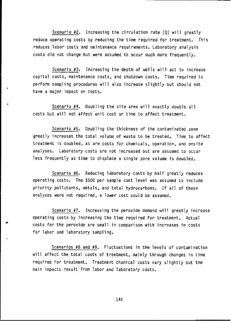
Scenario #2. Increasing the circulation rate (Q) will greatly
reduce operating costs by reducing the time required for treatment. Thisreduces labor costs and maintenance requirements. Laboratory analysis
costs did not change but were assumed to occur much more frequently.
Scenario #3. Increasing the depth of wells will act to increase
capital costs, maintenance costs, and shutdown costs. Time required toperform sampling procedures will also increase slightly but should nothave a major impact on costs.
Scenario #4. Doubling the site area will exactly double all
costs but will not affect unit cost or time to affect treatment.
Scenario #5. Doubling the thickness of the contaminated zonegreatly increases the total volume of waste to be treated. Time to affecttreatment is doubled, as are costs for chemicals, operation, and onsite
analyses. Laboratory costs are not increased but are assumed to occurless frequently as time to displace a single pore volume is doubled.
Scenario #6. Reducing laboratory costs by half greatly reducesoperating costs. The $500 per sample cost level was assumed to includepriority pollutants, metals, and total hydrocarbons. If all of theseanalyses were not required, a lower cost could be assumed.
Scenario #7. Increasing the peroxide demand will greatly increaseoperating costs by increasing the time required for treatment. Actual
costs for the peroxide are small in comparison with increases in costsfor labor and laboratory sampling.
Scenarios #8 and #9. Fluctuations in the levels of contamination
will affect the total costs of treatment, mainly through changes in timerequired for treatment. Treatment chemical costs vary slightly but the
main impacts result from labor and laboratory costs.
141

Scenario #10. Reducing the number of personnel required at the
site will have a major impact on costs. However, many factors will
determine the minimum number of personnel feasible for a site. The level
of onsite analyses, the number of wells requiring sampling, the degree of
automation, 24-hour operation, and relevant health and safety standards
will all affect staffing needs.
Overall it can be seen that performing in situ treatment is a highly
labor-intensive activity. This is due primarily to the high degree of
monitoring necessary to evaluate peformance and modify opcration. This
analysis has shown that many variations in costs are possible, but in
general the costs for monitoring the system are much greater than
construction and operation. The costs of treatment chemicals are smaller
and variations do not have a major impact on the total cost of treatment.
142

SECTION VII
SUMMARY OF OBSERVATIONS
This section provides a summary of the major observations made
during the operation of the system at Kelly AFB.
* The installed system circulated groundwater with very few
mechanical problems and very little down time.
* Initial addition of nutrients and hydrogen peroxide to the
system resulted in an almost immediate permeability reduction
from about 1 x 10⁻⁴ cm/sec to I x 10- 5 cm/sec and a calcium
phosphate precipitate was found in all injection wells.
a The high levels of nutrients and hydrogen peroxide added during
treatment may have caused effects, such as permeability
reductions and calcium phosphate precipitation, that otherwise
may not have been observed if lower levels had been used.
* During the demonstration, the sum of TCE and PCE levels in sitegroundwater decreased from 4.0 ppm to 0.96 ppm, while DCE con-
centrations increased from 0.3 ppm to 1.4 ppm.0 Carbon dioxide concentrations in the system groundwater were of
a magnitude greater than the presumed background levels at thesite and were equivalent to as much as 30 percent of the peroxide
oxygen supplied to the system.* Mobilization of heavy metals (Sb, As, Cd, Pb, Ag, Zn, Tl) from
"the soils is indicated by the data, but metals were not detectedin the groundwater.
0 Heavy metals were found at the surface as sediments in several
pumping well discharge lines.
0 Chemical communication between injection and production wells
was of sufficient strength to indicate that circulation rate
counters natural groundwater flow.
143

Large uptake of ammonia and phosphate by the soil is indicated;
data indicate a higher uptake of phosphate than ammonia.
Correlation of similarities between laboratory and field tests
included: (1) permeability reduction, (2) heavy metals mobiliza-
tion from soil, (3) phosphate lag of chloride breakthrough,
(4) peroxide lag of phosphate breakthrough, (5) PCE and FCE de-
cline, and (6) DCE increase.
* Reduction in soil microbial counts over the life of the demon-
stration was observed.
# No reduction in production fluid microbial counts was observed.
0 Reduction in injection fluid microbial counts was observed, even
at reduced levels of peroxide addition and at no peroxide addition.
144

SECTION VIII
CONCLUSIONS
A. DEGRADATION RESULTS
Analysis of results indicates that the treatment system implemented
at Kelly AFB, Texas successfully enhanced in situ degradation of organiccontaminants. Biological degradation was the most likely method of con-
taminant reduction as evidenced by the following:
# Degradation of chlorinated aliphatics was measured and followed
known pathways for anaerobic biodegradation.
e Aerobic biodegradation of petroleum hydrocarbons was indicated,
but could not be quantified since the small amount of degradationpossible was much less than natural variations in hydrocarbon
concentrations.
* Evidence indicated that contaminants were degraded by both aerobic
and anaerobic mechanisms within the same treatment zone. Thisindicates that in situ treatment may be considered for use atsites with both aerobically and anaerobically degradable wastes.
B. SITE CHARACTERISTICS
The hydraulic conductivity of a site plays a major role in the
effective implementation of in situ treatment. It dictates the timerequired to complete treatment and, therefore, will greatly affect the
total cost of treatment. The field test at Kelly AFB, however, showedthat distribution of chemicals and enhancement of biodegredation are
technically achievable even in low permeability aquifers. Hydraulic
conductivity values at Kelly AFB were as low as 0.11 feet per day. In
145

situ treatment is achievable, therefore, at the many hazardous waste
sites located in shallow surface aquifers of low permeability.
C. TREATMENT CHENICALS
Injection of chemicals to the subsurface can result in many chemicalreactions other than those intended to enhance biodegredation. Some of
these reactions can adversely affect the effectiveness and efficiency of
in situ treatment. Reactions causing precipitation can clog infiltration
wells and the aquifer itself. The reaction between the injected nutrient
phosphate and the soil mineral calcium caused precipitation at Kelly AFB.
Changes in pH and Eh induced by biodegradation and reoxygenation can
cause dissolution and precipitation of iron. Injected nutrients and
peroxide can react with other inorganic and organic chemicals. Even if
these reactions do not result in a precipitate, they will reduce the amount
of chemicals available to enhance biodegredation.
Another result of chemical reactions due to in situ treatment is the
potential for mobilization of heavy metals. The metals may then be trans-
ported as very fine particles, which, if not controlled, can present the
threat of spreading contamination. This could preclude the usefulness of
in situ bioreclamation of sites which are contaminated with a mixture of
organics and heavy metals. However, with proper control of transport and
with appropriate removal of heavy metals from circulating groundwater,
mobilization of heavy metals could prove beneficial in that they could be
removed from the waste site and disposed of properly. Some of the effects
observed at the Kelly AFB site may have been due to the high levels of
chemicals (nutrients and hydrogen peroxide) added during the treatment pro-
cess. These effects may not occur if reduced levels of chemicals are added.
D. COST OF IN SITU TREATMENT
Costs for treating all of Site E-1 at Kelly AFB were calculated using
the worksheets in Section VI. These costs were calculated to be
146

approximately $100 per ton of contaminated soil or $4,800,000. The costs
of excavation and removal of this entire volume of soil were calculated
at $5,787,000 (based on historical costs at Kelly AFB: $18 per cubic yard
for excavation and loading; $55 per cubic yard for transportation; and $138
per cubic yard for disposal).
By calculating costs for in situ treatment, it is seen that the
largest cost items are for field labor and laboratory analysis. By
increasing the level of automation and decreasing the amount of laboratory
testing through suitable onsite facilities some savings will De realized.
However, increasing the amount of onsite analyses will increase the
staff requirements which may offset a significant portion of the savings.
Reducing the number and frequency of analyses performed will result in
the greatest cost savings but limit monitoring of system performance.
Even using conservative estimates, however, in situ treatment is cost
competitive with removal and provides a more desirable approach to site
cleanup.
E. SAMPLING AND ANALYSIS
Reducing the level of sampling and analysis to reduce costs may
present some difficulties in providing full treatment. It was demon-
strated at Kelly AFB that treatment activity over a site can be highly
variable, even over very small areas. Under such conditions it is neces-
sary to provide a very extensive sampling and analysis program to determine
the effectiveness of treatment and adjust the operation of the system
accordingly. Until much more is known about the specific mechanisms of
in situ treatment, extensive analysis will continue to be warranted
especially for future research efforts. Such efforts may warrant the use
of more complex equipment on site such as a GC/MS unit. This will help
to offset some of the high cost of chemical analyses. For future full-
scale effort, the cost of an onsite GC/MS and operator will probably not
be warranted.
147

SECTION IX
RECOMMENDATIONS
A. REQUIREMENTS FOR FULL-SCALE IN SITU BIODEGRADATION
Full-scale application of in situ biodegradation will probably re-
quire significantly longer periods of operation than at Kelly AFB in
order to achieve cleanup. Most cleanups will probably take between 2
and 5 years depending on the complexity and quantity of wastes. Somesites may require even longer than 5 years. After only 8 months
of operation, the PVC pipe used for the test at Kelly AFB had begun to
weather and was subject to cracking under stress. For operations lasting
several years, more durable construction materials would be recommended.
In addition, large, long-term operations may require large surge and/or
onsite storage capacities and should be highly automated to allow greater
operational control and flexibility and reduce the amount of field labor
necessa ry.
Sampling and analytical procedures will also play an important role
in the operation of full-scale treatment. Analytical costs may make up
as much as 25 percent of total costs for future applications of this
technology. Before operation begins, a cost-benefit analysis will need
to be performed to determine whether onsite or offsite analysis will
be used. The outcome of this analysis will be primarily determined by
the frequency of analysis required. The frequency of sampling and analysis
will probably be less for full-scale applications than for research pro-
jects and a full-time, onsite laboratory may not be required. For large
sites, however, a single sampling event may involve hundreds of samples.
In addition to onsite and contract laboratory options, laboratory equip-
ment may be rented during sampling events with a chemist assigned to the
site on an as-needed basis. Analyses performed in an onsite laboratory
148

not approved by EPA will probably require periodic confirmation at anapproved, contract laboratory.
The required frequency and completeness of groundwater and soil
sampling will be highly site-specific. Sampling efforts will be mostintense during startup of the system and as treatment nears completion.
Many options exist for handling performance of these analyses. Futureresearch programs will define the most efficient and effective means of
providing zdequate sampling and analysis for full-scale applications ofin situ biodegradation.
B. GENERIC COST MODEL
The cost model presented in Section VI was developed as a result of
experience gained at Kelly AFB. It is intended to provide an approximatecost for in situ treatment for comparison with other alternatives at any
site. Using the model at future sites will provide information that canbe used to refine the model to provide greater accuracy and flexibility
for a wide variety of conditions. It is recommended, therefore, that themodel be used for future research programs and improvements made to pro-
vide a simple, accurate means of calculating the cost of full-scale
applications.
C. FUTURE TESTS/RESEARCH NEEDS
The test at Kelly AFB evaluated only one specific means of accom-
plishing in situ treatment. Several problems were identified andnumerous questions were raised concerning various aspects of in situ
treatment. These problems and questions will need to be addressed in
future research efforts before in situ biodegradation can be used effec-tively at complex waste sites. This section discusscs the major issues
requiring further study.
149

1. Alternate Injection/Extraction Systems
The groundwater circulation system used at Kelly AFB is only
one method of delivering nutrients and oxygen to the subsurface. Other
methods for reinjection of groundwater include forced injection wells
and infiltration galleries. There may also be opportunities for less
conventional methods such as surface ponding to provide water infiltra-
tion and treatment of contamination close to the ground surface. Small-
scale tests similar to that performed at Kelly AFB would be useful in
determining the applicability of these and other potential methods.
Through numerous tests and research, it should be possible to
develop an optimum groundwater circulation system for a giver site. Such
a system would take full advantage of site characteristics and system
geometry to provide the most efficient means of providing nutrient and
peroxide distribution throughout the desired area.
2. Nutrient Selection
An optimum nutrient formulation will provide sufficient nutrients
to enhance growth of microorganisms without adversely affecting soil
permeability. The development of nutrient formulations will be highly
site-specific depending on soil chemistry and the microbes present at
the site. A number of different chemical formulations of nutrients
should be tested against various common soil types to develop guidelines
for nutrient selection under various site conditions.
It will still be necessary to perform site-specific tests with
nutrient formulations to develop the nutrient composition and flow
rate necessary to achieve optimal loading with minimal negative
impacts. In cases where sufficient nutrients may be present in the
soil, introduction of additional nutrients may not provide sufficient
benefit and should be avoided.
150

3. Use of Hydrogen Peroxide
The use of hydrogen peroxide as an oxygen source should be studi-
ed further at sites with mixed chemical wastes. Evidence at Kelly AFB
suggested that, in addition to aerobic biodegredation, anaerobic bio-
degradation and chemical oxidation were also taking place. Tests should
be performed to aetermine if, indeed, all three of these mechanisms are
working in the presence of hydrogen peroxide and how to best control the
introduction of hydrogen peroxide to provide optimal treatment of wastes
degraded by all three mechanisms.
4. Metals Mobilization
The mechanism and chemical factors that control the mobilization
and disposition of heavy metals during in situ treatment need to be
determined. Data from Kelly AFB indicated that fine particle transport,
possibly facilitated by surfactants, may have been responsible for metals
mobilization. Changes in Eh and pH also may have played a major role. In
addition, the high concentrations of nutrients and hydi-ogen peroxide added
may facilitate transport of the colloidal particles. Additional study is
required to develop ways of controlling this mobilization to either leave
the metals in place or remove them from the subsurface for treatment and
disposal.
5. Precipitation and Clogging
The mechanisms controlling precipitate formation and soil clogg-
ing during in situ treatment should be identified so that steps can be
taken to avoid the problem at future applications. The precipitate
identified at Kelly AFB was calcium phosphate resulting from chemical
interactions with the soil. Other possible sources of clogging included
biomass, air (oxygen) blocking due to hydrogen peroxide degradation, and
mobilization and deposition of fine particles. Iron precipitation might
have caused serious clogging problems if the flow rate through the system
had been higher. Composition of soils, mineralogy, and soil pH should be
151

studied to determine the effects on precipitation both with and without
the use of nutrients and oxygen.
6. Carbon Dioxide Monitoring
The accuracy of using carbon dioxide measurements as an indica-
tion of biological degradation should be studied at future sites. It is
necessary to quantify the relationship between production of carbon
dioxide due to biological degradation, chemical degradation, and carbo-
nate equilibrium. If successful, carbon dioxide monitoring could be used
as an inexpensive means of quantifying biodegradation during the operation
of in situ treatment systems.
7. Soil Column Testing
It is recommended that column permeability tests using site-spe-
cific contaminated soils and groundwater be used to quantify how specific
sites will react to in situ treatment. At Kelly AFB, these tests, in
combination with laboratory microcosm treatability studies, showed the
same effects as observed in the field operation: significant permeability
reduction; mobilization of metals from the soil; reductions in TCE and
PCE levels, and an increase in DCE concentrations; a lag in phosphate
transport relative to chloride; and a lag in peroxide transport relative
to phosphate. In future applications of in situ treatment the data
previously obtained with microcosm tests could be obtained during column
testing. These studies would constitute engineering design data for
proposed field tests.
It is recommended that future studies be conducted in two
phases. The first phase would address the technical issue of identify-
ing nutrient and peroxide concentrations that maximize the rate of supply
152

(circulation rate x concentration) of each. The second phase, using
optimum nutrient and peroxide concentrations would be for obtaining
measurements of changes in the organic and metal concentrations in the
column with time and changes within the column from a reducing to an
oxidizing environment.
153

REFERENCES
1. Rogoshewski, P. J. 1977. Land Spreading of Oily Wastes. Depart-ment of Environmental Sci.nces, Rutgers, The State University,New Brunswick, New Jersey,
2. Kincannon, C. B. 1972. Oily Waste Disposal by Soil CultivationProcess. EPA-R2-72-110. U.S. Environmental Protection Agency,Washington, D.C.
3. Raymond, R. L., J. 0. Hudson, and V. W. Jamison. 1975. "OilDegradation in Soil." Applied ani Environmental Microbiology,Vol. 31, No. 4, pp. 522-535.
4. Jamison, V. W., R. L. Raymond, and L1. 0. Hudson, Jr. 1975. "Bio-Degradation of High-octane Gasoli'ie in Groundwater." Develop-ments in Industrial Microbiology, American Institute of Bio-logical Sciences. Washington, D.C., p. 305-312.
5. Lee, M. D. and C. H. Ward. 1984a. "Reclamation of ContaminatedAquifers: Biological Techniques." In the 1984 Hazardous MaterialSpills Conference Proceedings: Prevention, Behavior, Control,and Cleanup of Spills and Waste Sites. Government Institutes,Inc., Rockville, Maryland.
6. Minugh, E. M., J. J. Patry, D. A. Keech, and W. R. Leek. 1983. "ACase History: Cleanup of a Subsurface Leak of Refined Product."Proceedings of the 1983 Oil Spill Conference, American PetroleumInstitute, Washington, D.C., pp. 397-403.
7. U.S. EPA. 1984. Case Studies 1-23: Remedial Response at HazardousWaste Sites. EPA-540/2 84-002 b. Municipal Environmental Re-search Laboratory, Cincinnati, Ohio.
8. Raymond, R. L., V. W. Jamison, J. 0. Hudson, R. E. Mitchell, andV. E. Farmer. 1978. Final Report: Field Application of Sub-surface Biodegradation of Gasoline in a Sand Formation. Pro-ject No. 387-77 American Petroleum Institute, Washington, D.C.
9. Texas Research Institute, Inc. 1982. Enhancing the MicrobialDegradation of Underground Gasoline by-'IncreasinJ AvailabTeOxygen. Final Report. American Petroleum Institute, Washing-ton, D.C.
10. Lee, M. D. and C. H. Ward. 1984b. Biological Methods for theRestoration of Contaminated Aquifers. Draft Report. NationalCenter for Groundwater Research, Rice University, Houston,Texas.
154

REFERENCES (CONTINUED)
11. Boyd, S. A., D. R. Shelton, D. Berry, and J. M. Tiedje. 1983."Anaerobic Biodegradation of Phenolic Compounds in DigestedSludge." Applied and Environmental Microbiology. Vol. 46,No. 1, pp. 50-54.
12. Bouwer, E. J., B. E. Rittman, and P. L. McCarty. 1981. "AnaerobicDegradation of Halogenated 1- and 2-Carbon Organic Compounds."Environmental Science and Techpology, Vol. 15, No. 5, pp. 596-599.
13. Bouwer, E. J. and P. 0. McCarty. 1983. "Transformations of 1-and 2-Carbon Halogenated Aliphatic Organic Compounds UnderMethanogenic Conditions." Applied and Environmental Micro-biology. Vol. 45, No. 4, pp. 1286-1294.
14. Bouwer, E. J. and P. L. McCarty. 1983. "Transformations of Halo-genated Organic Compounds Under Denitrification Conditions."Applied and Environmental Microbiology. Vol. 45, No. 4, pp.1295-1298.
15. Parsons, F., P. R. Wood, and J. DeMarco. 1984. "Transformationsof Tetrachloroethane and Trichlorethene in Microcosms and Ground-water." Journal of the American Water Works Association. Febru-ary 1984, pp. 56-59.
16. Wilson, J. T., J. F. McNabb, D. L. Balkwill, and W. C. Ghiorse.1983. "Enumeration and Characterization of Bacteria Indigenousto a Shallow Water-Table Aquifer." Groundwater, Vol. 21, No. 2,pp. 134-142.
17. Wilson, J. T., J. F. McNabb, B. H. Wilson, and M. J. Noonan.1983. "Biotransformation of Selected Organic Pollutants inGroundwater." Developments in Industrial Microbiology, Volume24, pp. 225-234. Society of Industrial Microbiology, Arlington,Virginia.
18. Product Literature, LaMotte Chemical Products Co., P.O. Box 329,Chestertown, Maryland 21620.
19. Product Literature, Simplex Soil Testing Outfit, The EdwardsLaboratory, P.O. Box 318, Norwalk, Ohio.
20. Katz, D. L., et al. Movement of Underground Water in Contactwith Natural Gas. American Gas Association, New York, New York,February, 1963, p. 130.
155

REFERENCES (CONCLUDED)
21. Scheidegger, A. E. The Physics of Flow Through Porous Media.University of Toronto Press, 1963, p. 202.
22. Cooper, D. G. Biosurfactants and Enhanced Oil Recovery Applicationto Heavy Oils, pp. 112-113.
156