Basel Committee on Banking Supervision Working … Working Papers of the Basel Committee on Banking Supervision contain analysis carried out by experts of the Basel Committee or its

Basel Committee on Banking Supervision

Working Paper No 26

Foundations of the standardised approach for measuring counterparty credit risk exposures

August 2014 (rev. June 2017)

The Working Papers of the Basel Committee on Banking Supervision contain analysis carried out by experts of the Basel Committee or its working groups. They may also reflect work carried out by one or more member institutions or by its Secretariat. The subjects of the Working Papers are of topical interest to supervisors and are technical in character. The views expressed in the Working Papers are those of their authors and do not represent the official views of the Basel Committee, its member institutions or the BIS. This publication is available on the BIS website (www.bis.org).

© Bank for International Settlements 2017. All rights reserved. Brief excerpts may be reproduced or translated provided the source is cited.

ISSN 1561-8854

http://www.bis.org/

Foundations of the standardised approach for measuring counterparty credit risk exposures iii

Contents

Equation Chapter 1 Section 1Foundations of the standardised approach for measuring counterparty credit risk exposures ...................................................................................................................................................... 1

1. General structure of the SA-CCR .............................................................................................................................. 1

1.1 Exposure at default ........................................................................................................................................................ 1

1.2 Replacement cost ........................................................................................................................................................... 2

1.3 Potential future exposure ............................................................................................................................................ 3

2. General framework for add-ons ................................................................................................................................ 3

2.1 Assumptions and set-up .............................................................................................................................................. 3

2.2 Add-ons for unmargined netting sets .................................................................................................................... 4

2.3 Add-ons for margined netting sets ......................................................................................................................... 5

3. Structure of add-on calculations .............................................................................................................................. 6

3.1 Trade-level add-ons ....................................................................................................................................................... 6

3.2 Add-on aggregation ...................................................................................................................................................... 7

4. Add-on calculations by asset class .......................................................................................................................... 8

4.1 Interest rate ....................................................................................................................................................................... 8

4.2 Foreign exchange............................................................................................................................................................ 9

4.3 Credit ................................................................................................................................................................................... 9

4.4 Equities .............................................................................................................................................................................. 10

4.5 Commodities................................................................................................................................................................... 10

5. Multiplier .......................................................................................................................................................................... 11

6. Calibration........................................................................................................................................................................ 13

6.1 Correlations between IR maturity buckets .......................................................................................................... 14

6.2 Deltas for CDO ............................................................................................................................................................... 18

References .......................................................................................................................................................................................... 20

Foundations of the standardised approach for measuring counterparty credit risk exposures 1

Foundations of the standardised approach for measuring counterparty credit risk exposures

This technical paper explains modelling assumptions that were used in developing the standardised approach for measuring counterparty credit risk exposures (SA-CCR). The paper also clarifies certain aspects of the SA-CCR calibration that are not discussed in the final standard that was published in March 2014 (revised April 2014).1 The language used to describe the SA-CCR in this paper may differ somewhat from the language used in the final standard. For example, the paper uses concepts that are not present in the final standard such as trade-level add-ons and single-factor subsets of hedging sets. Furthermore, it does not use the concept of effective notional, which is employed in the standard. The purpose of these adaptations is to emphasise the common aggregation framework that underpins the SA-CCR add-on formulas for different asset classes.

1. General structure of the SA-CCR

1.1 Exposure at default

The SA-CCR specifies exposure at default (EAD) measured at a netting set level. The target EAD measure for a netting set under the SA-CCR is the corresponding EAD measure under the Internal Model Method (IMM), given by the product of multiplier α (alpha) and Effective Expected Positive Exposure (EEPE). Under the SA-CCR, the netting-set-level EEPE is represented as the sum of two terms: the replacement cost (RC) and the potential future exposure (PFE). Thus, EAD using SA-CCR is calculated via

( )EAD RC PFEα= ⋅ + (1)

where the multiplier alpha is set to the default IMM value, 1.4α = .

While the Current Exposure Method (CEM) also represents exposure as the sum of the RC and the PFE terms, Equation (1) differs from EAD using CEM in two important respects:

• The SA-CCR incorporates the multiplier alpha that (conceptually) converts EEPE into a loan equivalent exposure (see ISDA-TBMA-LIBA (2003); Canabarro, Picoult and Wilde (2003); and Wilde (2005)).

• The CEM specifies RC and PFE only for the unmargined case, while the SA-CCR includes formulations of RC and PFE that differ for margined and unmargined cases.

The approach to developing the SA-CCR was to simply reflect the RC and PFE for particular asset classes. RC represents a conservative estimate of the amount the bank would lose if the counterparty were to default immediately. It should be noted that margining practices are becoming more complicated over time and the approach to replacement cost reflects the diversity of margining practices that are common in the market. The PFE component reflects increases in exposure that could occur over time. PFE is related to volatility that is observed in the asset class.

1 The final standard can be retrieved from http://www.bis.org/publ/bcbs279.pdf.

http://www.bis.org/publ/bcbs279.pdf

2 Foundations of the standardised approach for measuring counterparty credit risk exposures

1.2 Replacement cost

For unmargined netting sets, RC represents the loss that would occur if the counterparty defaulted immediately. Suppose that a bank has a netting set of trades with a counterparty with the current mark-to-market (MTM) value V . If the counterparty were to default immediately, the loss for the bank would be equal to the greater of V and zero,2 so that RC is given by max{ ;0}V .

There may be cases when an unmargined netting set is supported by collateral other than variation margin. All such collateral is a form of independent collateral amount (ICA) that is posted at trade inception. Generally, a bank can both receive and post ICA. Received ICA reduces the RC, as it can be used to offset losses in the event of a counterparty default. Posted ICA can be lost in the event of the counterparty default, unless it is segregated in a bankruptcy-remote account. Thus, the bank’s net ICA position, or NICA, for a netting set is calculated via aggregating all received ICA with positive sign and all posted non-segregated ICA with the negative sign. Since all collateral in an unmargined netting set has the form of ICA (ie no variation margin is exchanged), the entire collateral amount is given by NICA.

The RC is obtained by subtracting the current cash-equivalent value of collateral available to the bank using a one-year horizon, CE (1 year)C , from the netting set MTM value:

NoMargin CERC max{ (1 year);0}V C= − (2)

For non-cash collateral, the cash-equivalent value CE (1 year)C is obtained from the current MTM

value of collateral MTMC via application of an appropriate supervisory haircut (1 year)h for a one-year

time horizon according to the general haircut formula:

MTM MTMCE

MTM MTM

[1 ( )] if 0( )

[1 ( )] if 0C h t C

C tC h t C

⋅ − >= ⋅ + <

(3)

The haircut for a given time horizon accounts for a possibility of an unfavourable change of collateral value over that time horizon.

For a margined netting set, collateral generally consists of two parts: ICA (also known as initial margin) and variation margin (VM) that is posted and returned depending on the netting set MTM (see, for example, Gregory (2012, Chapter 5).

The SA-CCR sets the RC for a margined netting set equal to the maximum of the current RC and a conservative estimate of the future RC. The current RC is given by

CurrentMargin CERC max{ (MPR);0}V C= − (4)

where CE (MPR)C is the cash-equivalent value of collateral obtained from MTMC via application of

Equation (3) with time horizon t set equal to the margin period of risk (MPR).3 The future RC is interpreted as the loss that could occur if the counterparty defaulted at an unknown time point within the one-year capital horizon. Because of the uncertainty of the default time, the netting set MTM value – and, therefore, the true RC – is not known. The SA-CCR conservatively assumes that, at the time of default, the netting set MTM value is high enough to trigger a margin call. This would occur at the MTM level equal to the sum

2 See, for example, Pykhtin (2011).

3 MPR represents the time period over which exposure to counterparty may increase. For margined netting sets, this is the time between the last margin call that the counterparty would respond to prior its default and the closeout after the default. For unmargined trades, the time period is one year or the final maturity, consistent with the one-year time horizon generally used in the Basel accord.


of the threshold (TH) and the minimum transfer amount (MTA). If there is initial margin, the future RC is obtained by subtracting NICA from the margin call trigger level, resulting in

FutureMarginRC max{TH MTA NICA;0}= + − (5)

By taking the maximum of Equations (4) and (5) one obtains the RC for margined netting sets:

Margin CERC max{ (MPR);TH MTA NICA;0}V C= − + − (6)

Sometimes margin agreement thresholds are set at a very high level, which would lead to unreasonably high values of the replacement cost and, therefore, the EEPE. This issue is addressed in the SA-CCR by capping the EEPE of a margined netting set by the EEPE of an otherwise equivalent unmargined netting set.

1.3 Potential future exposure

The SA-CCR specifies the PFE as the product of the aggregate (ie netting-set-level) add-on and a multiplier ( )W ⋅ described in Section 5, dependent on the ratio of the netting set’s current collateral-adjusted MTM

value CEV C− to the add-on itself:

aggregateCEaggregatePFE AddOn

AddOnV CW − = ⋅

(7)

The aggregate add-on is an estimate of the netting set EEPE under the assumptions that no collateral is currently held or posted and that the current MTM values of all trades are zero. It is generally the case that PFE is highest for at-the-money netting sets. The multiplier reduces the value of PFE when the collateral-adjusted MTM is negative.

2. General framework for add-ons

2.1 Assumptions and set-up

The netting-set-level add-on represents a conservative estimate of the EEPE of the netting set under the following assumptions:

• The current MTM value of each trade is zero (ie trade is at-the-money, ATM).

• The bank neither holds nor has posted collateral for the netting set.

• There are no cash flows within the capital horizon of one year.

• The evolution process for MTM value of each trade follows arithmetic Brownian motion with zero drift and fixed volatility.

These assumptions are needed to obtain the linear dependence of the aggregate add-on on a single dynamic quantity – the volatility of the netting set MTM value. The most important benefit of this dependence is that one can aggregate add-ons from a trade level to a netting-set level as if they were standard deviations. Furthermore, the SA-CCR calibration can be reduced to making assumptions on volatilities and correlations of market risk factors that drive trade MTM values.

Using these assumptions, the MTM value of trade i at time t can be represented as

{ }( ) 1ii i iM tV t t Xσ≥= (8)


where {}1 ⋅ is the indicator function of a Boolean variable (it takes a value of 1 if the argument is TRUE and

value of 0 otherwise), iM is the remaining maturity, iσ is the volatility of the MTM value of trade i and

iX is a standard normal random variable.

Suppose that we know the correlations ijr between random variables iX and jX . Then, the

MTM value ( )V t of a netting set at time t can be expressed via

( ) ( )V t t t Yσ= (9)

where Y is a standard normal random variable and ( )tσ is the annualised normal volatility of the netting set at time t given by

{ } { }

12

,( ) 1 1

i jij i jM t M t

i jt rσ σ σ≥ ≥

= ∑ (10)

Note that, in spite of the assumption of fixed annualised volatility for MTM value of each trade, the annualised volatility ( )tσ of the netting set generally depends on time t because trades that mature

before time t do not contribute to ( )tσ .

2.2 Add-ons for unmargined netting sets

Expected exposure (EE) can be calculated for an unmargined netting set:

{ }no-marginEE ( ) E max ( ) ,0 (0) ( )t t t Y t tσ ϕ σ = = (11)

where ( )ϕ ⋅ is the standard normal probability density, so (0) 1 / 2ϕ π= . This value represents the average exposure of the netting set at time t . Cases where the netting set value is negative represent situations where the bank owes the counterparty and so the exposure is set to zero.

Conceptually, the unmargined aggregate add-on should be defined as the EEPE calculated from the EE profile of Equation (11). However, this would require calculating ( )tσ at several time points between zero and one year. To avoid this complexity, the consultative paper BCBS (2013) floored the remaining maturity of all trades by one year.4 The maturity floor is equivalent to replacing ( )tσ with (0)σ in Equation (11) whenever 1t ≤ year, which allows one to calculate the EEPE from Equation (11) in closed form:

1 year

no-margin no-marginaggregate

0

1 2AddOn EE ( ) (0) (0) 1 year1 year 3

t dt ϕ σ= =∫ (12)

Note that Equation (12) can be restated in terms of aggregation of trade-level add-ons rather than aggregation of trade-level volatilities:

12

no-margin no-margin no-marginaggregate

,AddOn r AddOn AddOnij i j

i j

= ∑ (13)

where add-on of trade i represents the EEPE of a netting set consisting of only trade i :

4 See Pykhtin (2014) for analysis of the BCBS (2013) proposals.


no-margin 2AddOn (0) 1 year3i iϕ σ= (14)

However, application of the one-year floor would result in unreasonably high trade-level add-ons for short-term trades. In particular, short-term trades would have a capability to offset long-term trades to a much greater extent that they should.5 To prevent this, the definition of the aggregate add-on for unmargined netting sets was kept in the form of Equation (13), but the definition of trade-level add-on was changed to accommodate maturities shorter than one year:

no-margin no-margin2AddOn (0) 1 year MF3i i iϕ σ= (15)

where maturity factor no-marginMFi is defined as

no-margin min{ ,1year}MF1year

ii

M= (16)

scales down the volatility of the trade MTM from one year to the trade remaining maturity iM for the

trades with 1yeariM < .

2.3 Add-ons for margined netting sets

For margined netting sets, the SA-CCR add-on is defined (in the spirit of the IMM Shortcut Method) as the expected increase of the netting set MTM over the MPR.6 Since the portfolio is assumed to have the current MTM equal to zero, the add-on for a margined netting set defined in this manner reduces to the value of the EE of an otherwise equivalent unmargined netting set at the time point equal to the MPR:

margin no-marginaggregateAddOn EE (MPR) (0) (0) MPRϕ σ= = ⋅ (17)

Similarly, for a margined netting set containing only trade i , the add-on is

marginAddOn (0) MPRi iϕ σ= (18)

Thus, one can replace aggregation of trade-level volatilities with aggregation of trade-level add-ons for both margined and unmargined netting sets via Equation (13) that we restate here for margined netting sets:

12

margin margin marginaggregate

,AddOn r AddOn AddOnij i j

i j

= ∑

Finally, trade-level margined add-ons in Equation (18) can be restated in exactly the same form as trade-level non-margin add-ons in Equation (15)

margin margin2AddOn (0) 1 year MF3i i iϕ σ= (19)

with differently defined maturity factors:

5 For example, to fully offset the risk of a one-year FX forward, it would be sufficient to book a very short-term FX forward or an

FX spot contract of the same notional in the opposite direction.

6 See BCBS (2006) and BCBS (2010). See also analysis in Gibson (2005) where the IMM Shortcut Method was first proposed.


margin 3 MPRMF2 1yeari = (20)

Thus, the entire difference between margined and unmargined trade-level add-ons resides in the maturity factors. Because of this, there will be no distinction made between margined and unmargined netting sets in the remainder of this paper when add-ons are discussed.

3. Structure of add-on calculations

For the purpose of the add-on calculation, each trade in the netting set is assigned to at least one of five asset classes: interest rate (IR), foreign exchange (FX), credit, equities and commodities. The designation should be made according to the nature of the primary risk factor (eg IR for most single currency IR swaps, FX for most cross-currency swaps, credit for most credit default swaps). For more complex trades, where it is difficult to determine a single primary risk factor, bank supervisors may require that trades be allocated to more than one asset class.

While the SA-CCR add-on formulas are asset class-specific, there are a number of common features for all asset classes. Most importantly, netting-set-level add-ons are calculated from trade-level add-ons via an aggregation procedure based on the general principles outlined in the previous section.

3.1 Trade-level add-ons

The SA-CCR does not directly operate with trade volatilities. Instead, the directional add-on ( trade)AddOn i

for each trade i of asset class a is given by the product of the following four quantities: directional delta

iδ , adjusted notional ( )aid , supervisory factor ( )SF a

i and maturity factor MFi :

( trade) ( ) ( )AddOn SF MFa ai i i i idδ= (21)

where maturity factor MFi is defined via Equation (16) for unmargined trades and via Equation (20) for

margined trades. Equation (21) is meant to be equivalent to Equations (15) and (19) with one difference: add-ons in Equation (21) can be negative. Negative add-ons are a means of accommodating negative correlations ijr in Equation (13) without using negative correlations explicitly. Comparing Equation (21)

with Equations (15) and (19) reveals that the SA-CCR approximates the trade-level volatility via

( )

( )3 SF | |2 (0)

aai

i i idσ δϕ

= ⋅ ⋅ (22)

where the first factor (the ratio) can be interpreted as the standard deviation of the primary risk factor at the one-year horizon.

The quantities that appear in Equation (21) are specified in the final standard for the SA-CCR. They have the following meaning:

• Directional delta iδ : Delta serves two purposes: it specifies the direction of the trade with the

respect to the primary risk factor (positive for long, and negative for short) and serves as the scaling factor for trades that are non-linear in the primary risk factor. Banks’ internal deltas are not allowed; standardised values are used instead. Trades that are not options or CDOs are assumed to be linear in the underlying risk factor and have delta of unit magnitude. For options, banks should use the Black-Scholes formula for delta as provided in the final standard. For CDOs,


a standardised formula provided in the standard text should be used with internal attachment and detachment points (this formula is discussed later in this paper).

• Adjusted notional ( )aid : While the definition of adjusted notional is asset class-specific, one can

generally state that adjusted notional quantifies the size of the trade. It is proportional to either a trade’s notional (as in the case of IR, FX and credit) or the current price of the underlying assets (as in the case of equity and commodity). For IR and credit derivatives, the adjusted notional is also proportional to the supervisory duration.

• Supervisory factor ( )SF ai : The supervisory factor is the supervisory value of EEPE of a netting set

consisting of a single linear trade (ie unit delta) of unit adjusted notional belonging to the same subclass of asset class a as trade i . Supervisory factors incorporate the volatility assumed by regulators for the primary risk factor. While the final standard specifies supervisory factors at specific subclasses within each asset class, conceptually the SA-CCR structure is very flexible: the method can be easily made more or less granular without changing the structure of the approach.

3.2 Add-on aggregation

Aggregation of trade-level add-ons to the netting set level is done by imposing a certain structure on the correlation matrix ijr in the aggregation formula given by Equation (13). A key add-on aggregation

concept of the SA-CCR is the notion of a hedging set. By definition, a hedging set is the largest collection of trades of a given asset class within a netting set for which netting benefits are recognised in the PFE add-on of the SA-CCR. No netting is recognised across hedging sets, so a netting-set-level add-on is calculated as a direct sum of the absolute values of hedging-set-level add-ons:

(no-margin) (HS)AddOn AddOnmm

=∑ (23)

where (HS)AddOnm is the add-on for hedging set m . Equation (23) is equivalent to assuming perfect

positive correlation between hedging set MTM values.

Hedging-set-level add-ons are obtained via the following two-step aggregation process that recognises netting within each hedging set. All trades of a hedging set are designated to single-factor subsets. It is assumed that all trades of a given single-factor subset are driven by the same market factor, so full offset is allowed for such trades:

(SFS) (trade)

SFSAddOn AddOn

j

j ii∈

= ∑ (24)

where ( trade)AddOn i is the directional add-on (ie add-ons for long and short trades have opposite signs)

for trade i described above and notation SFS ji∈ should be interpreted as all trades belonging to single-

factor subset j of a given hedging set.

Single-factor subsets are further aggregated to a hedging-set level under the assumption that, within a hedging set, risk factors driving single-factor subsets are imperfectly correlated:

12

(HS) (SFS) (SFS)

, HSAddOn AddOn AddOn

m

m jk j kj k

ρ∈

= ⋅ ⋅ ∑ (25)

where notation , HSmj k ∈ should be interpreted as all pairs of single-factor subsets belonging to the

same hedging set m of a given asset class, and correlations jkρ are prescribed by regulators.


The next section describes asset-class-specific aspects of the general framework outlined above. These aspects include the definition of adjusted notional along with the specification of hedging sets, single-factor subsets and correlation parameters.

4. Add-on calculations by asset class

4.1 Interest rate

Consider a fixed-for-floating IR swap as the most common example of an IR derivative. Suppose that swap i payments start at time iS , end at time iE and refer to notional ( )iN t at time t . In the continuous limit,

swap MTM value can be written as

[ ]swap

max{ , }

( ) SR ( ) FR ( )DF( , )i

i

E

i i i iS t

V t t N t dτ τ τ= − ∫ (26)

where SR ( )i t is the swap rate at time t , FR is the fixed rate and DF( , )t τ is the discount factor from time

τ to time t . The SA-CCR assumes that all variability of the swap MTM value results from changes of the swap rate, thus “freezing” the discount factor in the integral. The IR supervisory factor is meant to capture the one-year volatility of the swap rate, while the adjusted notional is meant to represent the value of the integral in Equation (26) at time 0t = . The SA-CCR approximates the integral by setting the adjusted notional equal to

(IR ) SDi i id N= ⋅ (27)

where iN is the average of the swap notional over the remaining life of the swap payments and SDi is

the supervisory duration given by

exp( ) exp( )SD exp( )

i

i

Ei i

iS

rS rErt dtr

− − −= − =∫ (28)

with the interest rate set to 0.05r = .

Interest rate hedging sets are specified as all IR trades of a netting set denominated in the same currency. Three single-factor subsets of a hedging set are defined via the range of the end date: (1)

1 yeariE ≤ ; (2) 1 year 5 yearsiE< ≤ ; (3) 5 yearsiE > . Thus, Equation (24) specifies the add-ons for

each of the three maturity buckets of a given currency. Correlations between the maturity buckets are set as follows: 12 23 70%ρ ρ= = and 13 30%ρ = (calibration of these correlations is discussed later in this

paper). Thus, in the case of IR, Equation (25) becomes:

( ) ( ) ( )2 2 2(CCY) (MB) (MB) (MB)

1 2 3

1(MB) (MB) (MB) (MB) (MB) (MB) 21 2 2 3 1 3

AddOn AddOn + AddOn AddOn

+1.4 AddOn AddOn 1.4 AddOn AddOn 0.6 AddOn AddOn

m= +

⋅ ⋅ + ⋅ ⋅ + ⋅ ⋅

(29)

where the notation “CCY” indicates that the hedging set is a currency and the notation “MB” indicates that the single-factor subsets are maturity buckets.


4.2 Foreign exchange

Consider a linear FX trade such as an FX forward between a foreign currency and the domestic currency. Assuming that the forward maturity is greater than one year (smaller maturities are accounted by maturity factors), volatility of the forward’s MTM value over the one-year horizon is independent of the forward’s maturity and is given by the product of the notional of the foreign leg converted to the domestic currency using the current FX spot rate and the one-year relative volatility of the FX spot rate. This example motivates specifying the adjusted notional according to7

(FX) foreigni id N= (30)

where foreigniN is the current value of the notional of the foreign currency leg of trade i measured in the

domestic currency. If both legs of a trade are in different foreign currencies, a conservative simplification is applied: Equation (30) should be calculated for both legs, and the maximum should be chosen.

An FX hedging set is specified as all trades of a netting set referencing the same pair of currencies. It is assumed that all FX trades of the same hedging set are driven by the same market factor, which is the FX spot rate for the hedging set’s currency pair. Thus, Equation (24) aggregates all trades of a given currency pair, and Equation (25) reduces to taking the absolute value of the single single-factor add-on:

(CCY pair) (SFS)1AddOn AddOnm = . When delta for FX trades is calculated, the trade direction within each

currency pair must be consistent (eg positive for all trades long GBP/EUR and negative for all trades short GBP/EUR).

4.3 Credit

MTM value of the most popular credit derivative, single-name or index credit default swap (CDS), can be represented in the form similar to Equation (26):

CDS contr

max{ , }

( ) CS ( ) CS ( )DF( , ) [1 EL ( , )]i

i

E

i i i i iS t

V t t N t t dτ τ τ τ = − − ∫ (31)

where CS ( )i t is the credit spread at time t , contrCSi is the contractual credit spread and EL ( , )i t τ is the

risk-neutral expected loss due to default(s) between time t and time τ per unit of notional.8 The supervisory factors for credit derivatives account for the one-year volatility of the credit spread. The adjusted notional for credit derivatives is meant to represent the value of the integral in Equation (31) at time 0t = . It was decided to ignore the difference between the integrals in Equations (26) and (31) and set the adjusted notional for credit derivatives equal to the one for IR derivatives given by Equations (27) and (28).

All credit trades of a given netting set represent a single hedging set. A single-factor subset is specified as all credit trades referencing the same entity (which can be either a single name or an index). Thus, Equation (24) aggregates all credit trades in a netting set that reference the same entity. Aggregation across entities is done assuming that each entity is driven by a single systematic risk factor and an idiosyncratic risk factor. The systematic factor loading for entity j is quantified via correlation jρ between

the full stochastic driver of credit spread of entity j and the systematic factor. This correlation is set to 50% for entities that are single names and to 80% for those that are indices. The pairwise correlation between two distinct entities j and k is given by the product j kρ ρ and can have the following values:

7 One can show that this specification is appropriate for another common example of FX linear trades – cross-currency swap.

8 In the case of single-name CDS, EL ( , )i t τ is the risk-neutral cumulative probability of default between t and τ .


25% between two single names; 40% between a single name and an index; 64% between two indices. Applying the single-factor assumption to Equation (25) results in the following add-on aggregation formula:

( ) ( )12

2(Entity) 2 (Entity)CD

2

AddOn AddOn 1 AddOnj j j jj jρ ρ

= ⋅ + − ⋅ ∑ ∑ (32)

The key features of credit derivatives that are captured are the maturity aspect and the basis risk. The single-factor model reflects the fact that, although credit spreads in general move together, there can be considerable idiosyncratic variation in a single name that limits the benefits of hedging a long CDS with one reference name with a short CDS referencing a different name. This strikes a balance between recognising diversification (which is greatest when correlation is zero) and hedging of dissimilar names (which is greatest when correlation is one).

4.4 Equities

For the simplest linear equity derivatives, such as equity forwards, volatility of the trade MTM value is equal to the product of the volatility of the stock (index) price and the number of units of stock (index) referenced by the trade. The volatility of the equity price can be approximated by the product of the current stock (index) price and the relative volatility of the stock (index) price. The supervisory factors for equity derivatives are meant to capture the relative volatility of the stock (index) price, while the adjusted notional is set equal to the product to the current stock (index) price and the number of units referenced by the trade.

Aggregation of equity derivatives is done in exactly the same manner as aggregation of credit derivatives. It is assumed that all trades in a netting set referencing the same entity (single name or index) are driven by the same factor, so Equation (24) is applied at an entity level. It is further assumed that stock prices and equity index values are driven by a single systematic factor with the same correlation values as for credit derivatives: 50% single names and to 80% for those that are indices. Thus, Equation (32) is used for aggregation of equity derivatives across entities.

This design captures the tendency of equity markets to move together, but limits the ability of different names to offset. Here again, a balance was struck between recognising diversification benefits and hedging benefits.

4.5 Commodities

For commodity derivatives, the arguments with respect to the volatility of the MTM value of linear contracts are similar to those used for equity derivatives above. The supervisory factors for commodity derivatives are meant to capture the relative volatility of the commodity price, while the adjusted notional is defined as the product of the current unit price (eg one barrel of oil) of the commodity referenced by the trade and the number of units referenced by the trade.

A commodity hedging set is specified as all trades of a netting set referencing the same broad category of commodity: energy, metals, agricultural, or other commodity. Single-factor subsets are specified as a specific commodity type: electricity, oil, gas, nickel, corn. Aggregation within commodity types is done via Equation (24). Specific commodity types are aggregated to a hedging set level using the same single-factor model that is used for credit and equity derivatives, but with the correlation parameter set to 40% for all commodity types. This results in the use of Equation (32), but interpreting j as a specific

commodity type with jρ set to 40% for all j .


5. Multiplier

Recall that a netting-set-level add-on is an estimate of the netting set PFE under the four assumptions stated in Section 2.1 of this paper: current MTM and collateral are equal to zero; there are no cash flows within the horizon; MTM follows zero-drift Brownian motion. Let us examine what would happen to the netting set PFE when the first two assumptions are relaxed, so that non-zero current MTM and collateral are allowed.

Let us consider a margined netting set. Generally, EE of a margined netting set is characterised by a full term structure calculated from9

[ ]marginEE ( ) E max{ ( ) ( ),0}t V t C t= − (33)

where ( )V t is the MTM value of the netting set at time t and ( )C t is the collateral available to the bank at time t . The SA-CCR does not attempt to model collateral dynamics through time and simply takes a single point MPRt = from the EE profile as the measure of exposure. Furthermore, the SA-CCR assumes that collateral is not exchanged during the MPR, so only non-cash collateral can change value over the MPR due to volatility of the collateral asset. The volatility of non-cash collateral is not modelled either: instead, a haircut is applied to the current collateral value MTMC to obtain a deterministic cash-equivalent

value CE (MPR)C , as described by Equation (3). Thus, the SA-CCR target measure of exposure for

margined netting sets is

[ ]marginCEEE (MPR) E max{ (MPR) (MPR),0}V C= − (34)

Under the assumption that a netting set’s MTM follows a driftless Brownian motion, the value of the MTM at the MPR can be described via

(MPR) (0) MPRV V Yσ= + (35)

where )0(σ is the volatility of the netting set MTM value at time 0 (ie counting all trades in the netting

set) and Y is a standard normal random variable.10 Substituting Equation (35) into Equation (34), calculating the expectation analytically results in:

[ ]margin CECE

CE

(MPR)EE (MPR) (MPR)(0) MPR

(MPR)(0) MPR(0) MPR

V CV C

V C

σ

σ ϕσ

−= − Φ

−

+

(36)

where ( )Φ ⋅ is the standard normal cumulative distribution function. The margined add-on in the form of

Equation (17) is obtained from Equation (36) by setting CE (MPR) 0V C− = :

marginaggregateAddOn (0) (0) MPRϕ σ=

To obtain the PFE, one needs to subtract the current replacement cost from the right-hand side of Equation (36). However, the SA-CCR does not give any credit to PFE reduction when the replacement cost is positive (ie margin margin

aggregatePFE AddOn= whenever CE (MPR) 0V C− ≥ ). For the

CE (MPR) 0V C− < case, Equation (36) produces the PFE because the current replacement cost is zero.

9 See, for example, Pykhtin (2010).

10 See Section 2.


To derive the SA-CCR multiplier, we need to express the PFE in terms of add-on rather than volatility. This is easily achieved by using Equation (17) to express (0)σ in terms of the margined add-on in Equation (36):

[ ]margin CECE margin

aggregate

marginaggregate CE

marginaggregate

(MPR)PFE (MPR) (0)AddOn

AddOn (MPR)(0)(0) AddOn

V CV C

V C

ϕ

ϕ ϕϕ

−= − ⋅Φ

−

+ ⋅

(37)

where Equation (37) is valid only for the CE (MPR) 0V C− < case.

By definition, the multiplier is the ratio of the PFE to the add-on. Combining the positive and negative collateralised MTM cases and using a shorthand notation

marginCE aggregate[ (MPR)] / AddOny V C= − , one obtains the “model” multiplier:

[ ] [ ]model

(0)( ) min 1, (0)

(0)y

W y y yϕ ϕ

ϕϕ

= Φ +

(38)

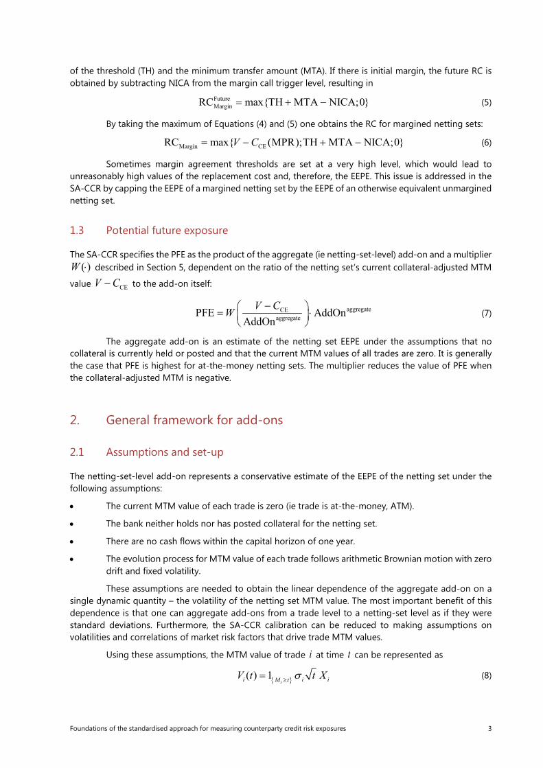
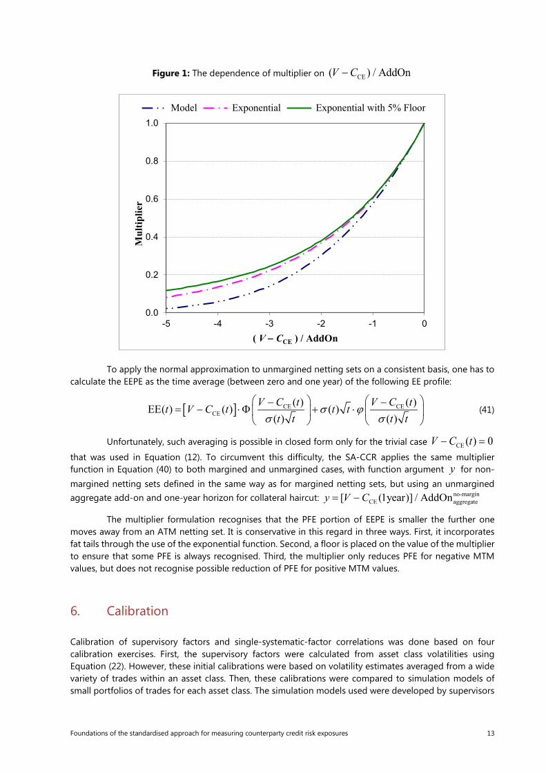
This function is shown by the dash-double-dotted curve in Figure 1.

The multiplier in Equation (38) is based on the assumption that the netting set future MTM value is normally distributed. However, MTM values of real netting sets are likely to exhibit heavier tail behaviour than the one of the normal distribution. To account for this possibility, a more conservative multiplier function was chosen:

exp ( ) min 1,exp2yW y =

(39)

where the factor of 2 appears in the denominator in order to match the slope of model ( )W y at 0y = . This

function is shown by the dash-dotted curve in Figure 1.

While the exponential multiplier in Equation (39) is significantly more conservative than the model-based multiplier in Equation (38), concerns were raised that the multiplier would still approach zero with infinite overcollateralisation. To address this concern, a floor F was added to the exponential multiplier in a manner that preserves the function slope at the origin:

SA-CCR ( ) min 1, (1 )exp2(1 )

yW y F FF

= + − −

(40)

The solid curve in Figure 1 shows this function with 5%F = currently chosen in the SA-CCR.


Figure 1: The dependence of multiplier on CE( ) / AddOnV C−

To apply the normal approximation to unmargined netting sets on a consistent basis, one has to calculate the EEPE as the time average (between zero and one year) of the following EE profile:

[ ] CE CECE

( ) ( )EE( ) ( ) ( )( ) ( )

V C t V C tt V C t t tt t t t

σ ϕσ σ

− −= − ⋅Φ + ⋅

(41)

Unfortunately, such averaging is possible in closed form only for the trivial case CE ( ) 0V C t− =

that was used in Equation (12). To circumvent this difficulty, the SA-CCR applies the same multiplier function in Equation (40) to both margined and unmargined cases, with function argument y for non-margined netting sets defined in the same way as for margined netting sets, but using an unmargined aggregate add-on and one-year horizon for collateral haircut: no-margin

CE aggregate[ (1year)] / AddOny V C= −

The multiplier formulation recognises that the PFE portion of EEPE is smaller the further one moves away from an ATM netting set. It is conservative in this regard in three ways. First, it incorporates fat tails through the use of the exponential function. Second, a floor is placed on the value of the multiplier to ensure that some PFE is always recognised. Third, the multiplier only reduces PFE for negative MTM values, but does not recognise possible reduction of PFE for positive MTM values.

6. Calibration

Calibration of supervisory factors and single-systematic-factor correlations was done based on four calibration exercises. First, the supervisory factors were calculated from asset class volatilities using Equation (22). However, these initial calibrations were based on volatility estimates averaged from a wide variety of trades within an asset class. Then, these calibrations were compared to simulation models of small portfolios of trades for each asset class. The simulation models used were developed by supervisors

0.0

0.2

0.4

0.6

0.8

1.0

-5 -4 -3 -2 -1 0

Mul

tiplie

r

( V − CCE ) / AddOn

Model Exponential Exponential with 5% Floor


and banks’ own IMM models. Lastly, to ensure that the SA-CCR was applicable to large portfolios, a quantitative impact study was conducted where banks compared the results for their own portfolios using SA-CCR, IMM and CEM. The final calibration considers the results of all of these exercises. The final parameter calibrations are provided in the final standards text. The rest of this section will focus on two specific aspects of the SA-CCR calibration: correlations between IR maturity buckets and deltas for CDO tranches.

6.1 Correlations between IR maturity buckets

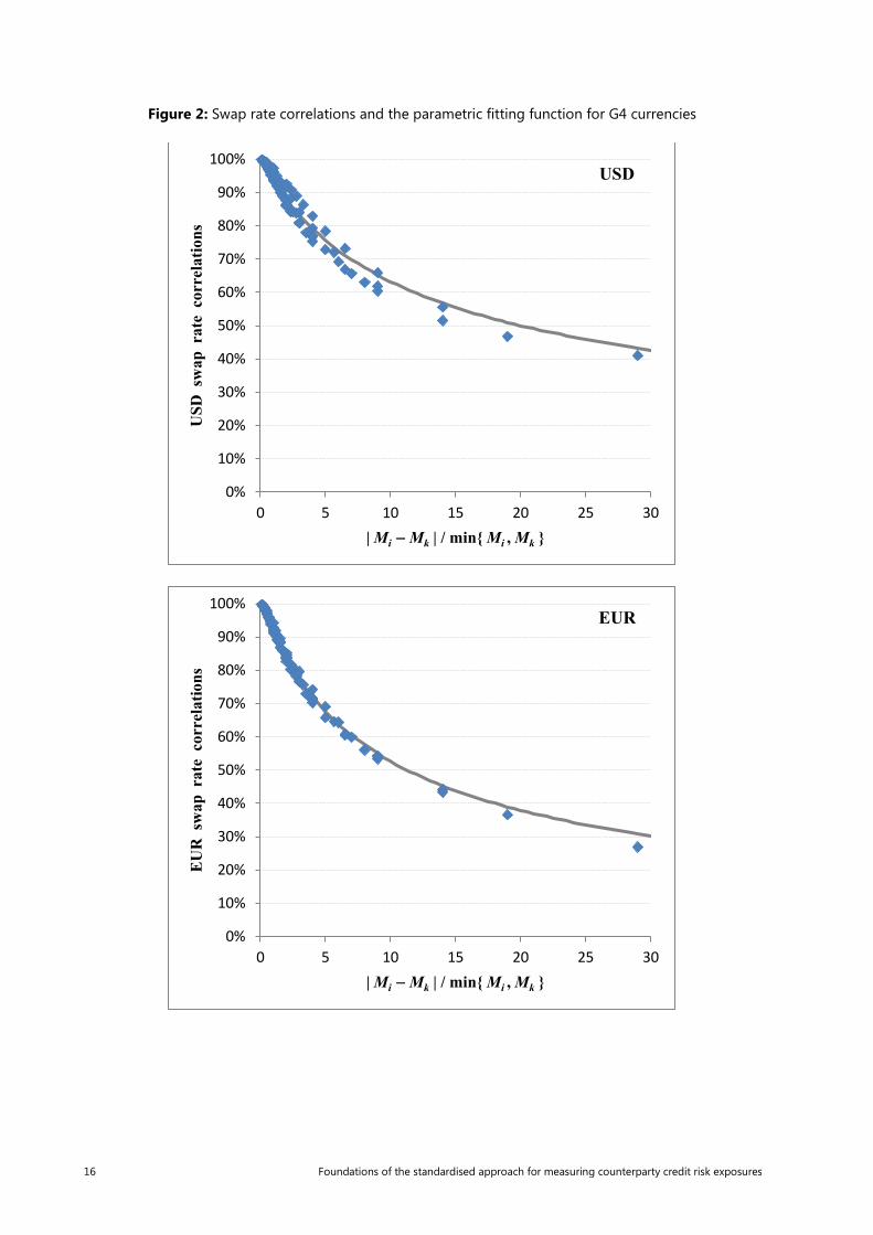
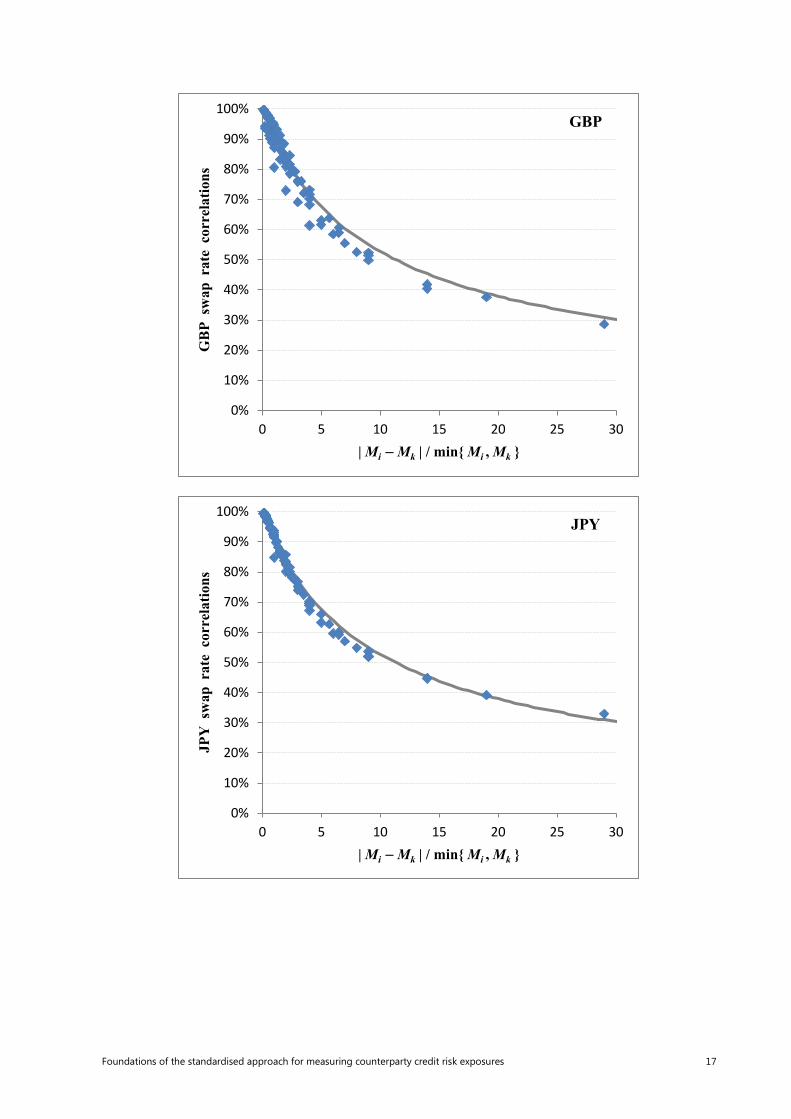
Generally, the correlation between MTM values of two IR trades referencing the same IR curve depends on four time parameters: the start and end dates of either trade as they are defined in Section 4.1 of this paper. However, this four-dimensional problem is not tractable within a simple non-model approach. To simplify the problem, two time dimensions were eliminated by assuming that the start date is equal to zero for all trades.11 Now one can use historical correlations between swap rates of different tenors as proxies for correlations between MTM values of trades with different remaining maturities.

Historical correlations between weekly changes of swap rates of different tenors (between one year and 30 years) for each of four major currencies (USD, EUR, GBP and JPY) were calculated for the time period from January 1, 2005 to December 31, 2009. To find a parametric function of two tenors that adequately describes the historical correlations calculated for each currency, a two-step procedure was followed:

• Reducing the two tenor dimensions into a single effective dimension: The data plotted as a function of this effective dimension should lie on a smooth curve rather than be scattered. Data points in Figure 2 show the historical correlations as a function of | | / min{ , }i k i kM M M M− for the four

major currencies, where iM is the tenor of swap rate i . One can see that the data points group

along smooth lines in all four plots, so this combination of tenors is a good approximation for the effective single dimension.

• Finding a simple parametric fitting function of the effective dimension: The solid curve in each of the panels of Figure 2 represents the function given by

1

| |1min{ , }

ik

i k

i k

bM Ma

M M

ρ = −+

(42)

with the following values of the parameters: ( 0.15a = ; 0.5b = ) for USD and ( 0.15a = ; 0.7b = ) for EUR, GBP and JPY.

Since values 0.15a = and 0.7b = used in Equation (42) adequately describe three out of four major currencies, it was decided to apply these values to all currencies.

One could apply Equation (42) directly to calculate correlations between any pair of IR trades of the same hedging set (ie the same currency). However, this approach would involve a double summation across the trades, which could become problematic for large netting sets. To overcome this difficulty, it was decided to create maturity buckets and treat all trades within a given maturity bucket as being driven by a single factor. Under this approach, the double summation only applies to a small fixed number of buckets rather than to a potentially large number of individual trades. The SA-CCR specifies three maturity buckets: (1) 0–1 year (midpoint is 0.5 year); (2) 1–5 years (midpoint is three years); (3) above five years (midpoint is set to 18 years). Applying Equation (42) with parameters 0.15a = and 0.7b = to the midpoints of these maturity buckets yields the following correlation values: 68% between buckets 1 and 2

11 Since real IR portfolios are dominated by ongoing IR swaps, this assumption should not lead to large distortions.


and 2 and 3 and 28% between buckets 1 and 3. Rounding these numbers to 70% and 30%, respectively, results in Equation (29).


Figure 2: Swap rate correlations and the parametric fitting function for G4 currencies

0%

10%

20%

30%

40%

50%

60%

70%

80%

90%

100%

0 5 10 15 20 25 30

USD

sw

ap r

ate

cor

rela

tions

| Mi − Mk | / min{ Mi , Mk }

USD

0%

10%

20%

30%

40%

50%

60%

70%

80%

90%

100%

0 5 10 15 20 25 30

EU

R s

wap

rat

e c

orre

latio

ns

| Mi − Mk | / min{ Mi , Mk }

EUR


0%

10%

20%

30%

40%

50%

60%

70%

80%

90%

100%

0 5 10 15 20 25 30

GB

P sw

ap r

ate

cor

rela

tions

| Mi − Mk | / min{ Mi , Mk }

GBP

0%

10%

20%

30%

40%

50%

60%

70%

80%

90%

100%

0 5 10 15 20 25 30

JPY

sw

ap r

ate

cor

rela

tions

| Mi − Mk | / min{ Mi , Mk }

JPY


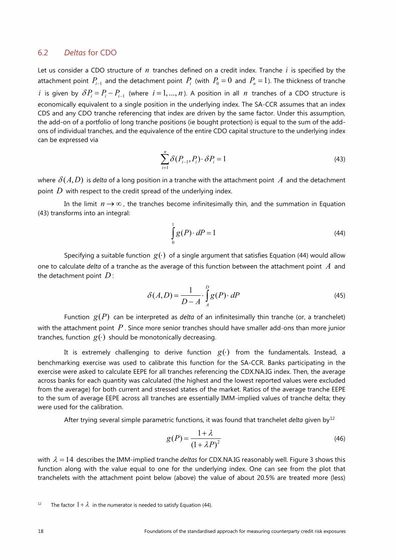
6.2 Deltas for CDO

Let us consider a CDO structure of n tranches defined on a credit index. Tranche i is specified by the attachment point 1iP− and the detachment point iP (with 0 0P = and 1nP = ). The thickness of tranche

i is given by 1i i iP P Pδ −= − (where 1, ...,i n= ). A position in all n tranches of a CDO structure is

economically equivalent to a single position in the underlying index. The SA-CCR assumes that an index CDS and any CDO tranche referencing that index are driven by the same factor. Under this assumption, the add-on of a portfolio of long tranche positions (ie bought protection) is equal to the sum of the add-ons of individual tranches, and the equivalence of the entire CDO capital structure to the underlying index can be expressed via

11

( , ) 1n

i i ii

P P Pδ δ−=

⋅ =∑ (43)

where ( , )A Dδ is delta of a long position in a tranche with the attachment point A and the detachment

point D with respect to the credit spread of the underlying index.

In the limit n →∞ , the tranches become infinitesimally thin, and the summation in Equation (43) transforms into an integral:

1

0

( ) 1g P dP⋅ =∫ (44)

Specifying a suitable function ( )g ⋅ of a single argument that satisfies Equation (44) would allow

one to calculate delta of a tranche as the average of this function between the attachment point A and the detachment point D :

1( , ) ( )

D

A

A D g P dPD A

δ = ⋅ ⋅− ∫ (45)

Function ( )g P can be interpreted as delta of an infinitesimally thin tranche (or, a tranchelet)

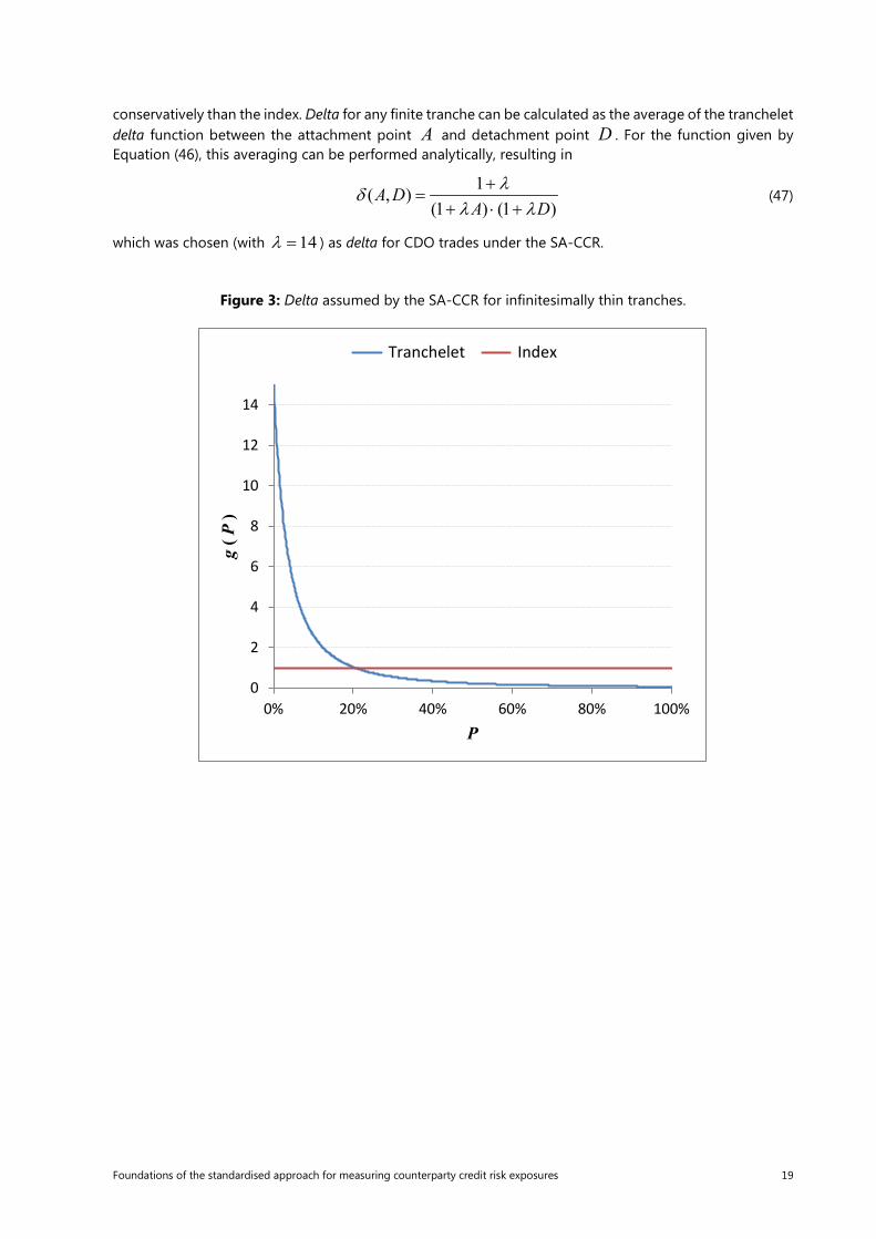
with the attachment point P . Since more senior tranches should have smaller add-ons than more junior tranches, function ( )g ⋅ should be monotonically decreasing.

It is extremely challenging to derive function ( )g ⋅ from the fundamentals. Instead, a benchmarking exercise was used to calibrate this function for the SA-CCR. Banks participating in the exercise were asked to calculate EEPE for all tranches referencing the CDX.NA.IG index. Then, the average across banks for each quantity was calculated (the highest and the lowest reported values were excluded from the average) for both current and stressed states of the market. Ratios of the average tranche EEPE to the sum of average EEPE across all tranches are essentially IMM-implied values of tranche delta; they were used for the calibration.

After trying several simple parametric functions, it was found that tranchelet delta given by12

2

1( )(1 )

g PPλλ+

=+

(46)

with 14λ = describes the IMM-implied tranche deltas for CDX.NA.IG reasonably well. Figure 3 shows this function along with the value equal to one for the underlying index. One can see from the plot that tranchelets with the attachment point below (above) the value of about 20.5% are treated more (less)

12 The factor 1 λ+ in the numerator is needed to satisfy Equation (44).


conservatively than the index. Delta for any finite tranche can be calculated as the average of the tranchelet delta function between the attachment point A and detachment point D . For the function given by Equation (46), this averaging can be performed analytically, resulting in

1( , )

(1 ) (1 )A D

A Dλδ

λ λ+

=+ ⋅ +

(47)

which was chosen (with 14λ = ) as delta for CDO trades under the SA-CCR.

Figure 3: Delta assumed by the SA-CCR for infinitesimally thin tranches.

0

2

4

6

8

10

12

14

0% 20% 40% 60% 80% 100%

g( P

)

P

Tranchelet Index


References

Basel Committee on Banking Supervision (1988): International convergence of capital measurement and capital standards, July.

——— (2006): International convergence of capital measurement and capital standards: A revised framework, June.

——— (2010): Basel III: A global regulatory framework for more resilient banks and banking systems, December.

——— (2013): The non-internal model method for capitalising counterparty credit risk, consultative document, June.

Canabarro, E, E Picoult and T Wilde (2003): “Analysing counterparty risk”, Risk, September, pp 117–22.

Gibson, M (2005): “Measuring counterparty credit exposure to a margined counterparty” in M Pykhtin (ed), Counterparty credit risk modelling, Risk Books.

Gregory J (2012): Counterparty credit risk and credit value adjustment, Wiley.

ISDA-TBMA-LIBA (2003): Counterparty risk treatment of OTC derivatives and securities financing transactions, June, www.isda.org/c_and_a/pdf/counterpartyrisk.pdf.

Pykhtin, M (2010): “Collateralised credit exposure” in E Canabarro (ed), Counterparty credit risk, Risk Books.

——— (2011): “Counterparty risk management and valuation” in T Bielecky, D Brigo and F Patras (eds), Credit risk frontiers, Wiley.

——— (2014): “The non-internal model method for counterparty credit risk” in E Canabarro and M Pykhtin (eds), Counterparty risk management, Risk Books.

Wilde, T (2005): “Analytic methods for portfolio counterparty risk” in M Pykhtin (ed), Counterparty credit risk modelling, Risk Books.

http://www.isda.org/c_and_a/pdf/counterpartyrisk.pdf

Documents

Basel Committee on Banking Supervision Working … Working Papers of the Basel Committee on Banking Supervision contain analysis carried out by experts of the Basel Committee or its