Basic Data Analysis Using ROOT - Nevis Laboratoriesseligman/root-class/Root...Basic Data Analysis Using ROOT A guide to this tutorial If you see a command in this tutorial is preceded

Basic Data Analysis Using ROOT

A guide to this tutorial

If you see a command in this tutorial is preceded by "[]", it means that it is a ROOTcommand. You should type that command into the ROOT program as appropriate,without the "[]" symbols. For example, if you see

[] .x treeviewer.C

it means to type ".x treeviewer.C" at a ROOT command prompt.

If you see a command in this tutorial is preceded by ">", it means that it is a UNIXcommand. You should type that command into UNIX, not into ROOT, and without the">" symbol. For example, if you see

> man less

it means to type "man less" at a UNIX command prompt.

Most of the lessons have time estimates at the top. These are only rough estimates;some students take 20 minutes to go through a lesson labeled "15 minutes", others takeonly 7 minutes. Don’t be too concerned about time; the important thing is for you to learnsomething, not to punch a time clock.

You can find this tutorial in Postscript and PDF format (along with links to the samplefiles) at <http://www.nevis.columbia.edu/~seligman/root−class/>. You can find additionalROOT tutorials at <http://root.cern.ch/root/Publications.html>.

Getting started on Linux

Use your account name and password to login. If your screen is just showing text(without any graphics at all), then type "startx" to run X−windows. Click once on theNetscape icon at the bottom of the screen to start Netscape.

Type the following URL in the "Location" field of the web browser: http://root.cern.ch/.This is the ROOT web site. You’ll be coming back here often, so be sure to bookmarkthis site.

02−Aug−2001 Basic Data Analysis Using ROOT Page 1 of 23

A Brief Intro to LinuxIf you’re already reasonably familiar with Linux or UNIX in general, skip this section.

You can spend a lifetime learning Linux; I’ve been working with UNIX since 1993 and I’mstill learning something new every day. The commands below barely scratch the surface.You may to look at UNIXhelp <http://www.geek−girl.com/Unixhelp/>, UNIX is a Four−Letter Word <http://www.msoe.edu/~taylor/4ltrwrd/>, and the usually out−of−dateinformation I maintain at <http://www.nevis.columbia.edu/software/>.

To copy a file: use the "cp" command.

For example, to copy the file "example.C" from the directory "~seligman/root−class" toyour current working directory, type:

> cp ~seligman/root−class/example.C $cwd

In UNIX, the variable $cwd means your "current working directory". (I know that a period(.) is the more usual abbreviation, but many students kept missing the period the firsttime I taught this class.)

To look at the contents of a text file: Use the "less" command.

This command is handy if you want to quickly look at a file without editing it. If the nameof the command seems puzzling, it may help to know the "more" command also displaysthe contents of a text file, and the "less" command was created as more powerful versionof "more". So to quickly look at the contents of file example.C, type:

> less example.C

While "less" is running, type a space to go forward one screen, type "b" to go backwardone screen, type "q" to quit, and type "h" for a complete list of commands you can use.

To get help on any UNIX command: type "man <command−name>".

While "man" is running, you can use the same navigation commands as "less". Forexample, to learn about the "ls" command, type:

> man ls

To edit a file: use the "emacs" command. (If you’re already familiar with another editor,such as "pico", you can use it instead.)

You will almost aways want to add an ampersand (&) to the end of any "emacs"command; the ampersand means to run the command as a separate process. So to editthe file example.C, type:

> emacs example.C &

The "emacs" environment is complex, and you can spend a lifetime learning it. (AlreadyI’ve spent two of your lifetimes, and the class has just started!) You can get around byusing the mouse to move the cursor and look at the menus. As soon as you can(probably not during this class), you should take the Emacs tutorial by selecting it underthe "Help" menu.


Starting ROOT (5 minutes)Before you start using ROOT, you have to type the following command:

> setup root

The command "setup root" sets some Unix environment variables and modifies yourcommand and library paths. If you feel a need to remove these changes, use thecommand "unsetup root".

One of the variables that is set is $ROOTSYS. This will be helpful to you if you’refollowing one of the examples in the ROOT User’s Guide. For example, if you’re told tofind a file in $ROOTSYS/tutorials, you’ll be able to do this only after you’ve typed "setuproot".

You have to execute the "setup root" command only once, but you must do it each timeyou login to Linux. If you wish this command to be automatically executed when youlogin, you can add it to the .mycshrc file in your home directory.

You are going to need to have at least two windows open during this class. One windowI’ll call your "ROOT command" window; this is where you’ll run ROOT. The other is aseparate "UNIX command" window. Create a second window with the followingcommand; don’t forget the ampersand (&):

> xterm &

It doesn’t matter which of these two windows is your ROOT window or your UNIXcommand window.

To actually run ROOT, just type:

> root

The window in which you type this command will become your ROOT command window.

First you’ll see the orange−and−red ROOT window appear on your screen. It will thendisappear, and a brief "Welcome to ROOT" display will be written on your commandwindow.

If you don’t see the orange−and−red ROOT window appear briefly on your screen, itmeans that X−windows is not functioning properly on your system; tell Bill Seligman.However, this is unlikely, since the "xterm" command would have failed if X−windowswere not working.

Click on the ROOT window to select it, if necessary.

You can type "?" (or ".h") to see a list of ROOT commands... but you’ll probably getmore information than you can use right now. Try it and see.

The most important ROOT line command you need to know is how to quit ROOT. Toexit ROOT, type ".q". Do this now, then start ROOT again, just to make sure you can doit.


Plotting a function (15 minutes)This example is based on the first example in Chapter 2 of the ROOT Users Guide (page15). I emphasize different aspects of ROOT than the Users Guide, and it’s a good ideato go over both the example in the Guide and the one below.

Let’s plot a simple function. Start ROOT and type the following at the prompt:

[] TF1 f1("func1","sin(x)/x",0,10)

[] f1.Draw()

Note the use of C++ syntax to invoke ROOT methods. (Page 16 of the ROOT UsersGuide has a discussion of this.)

If you have a keen memory (or you type ".h" on the ROOT command line), you’ll noticethat neither TF1 nor any of its methods are listed as commands, nor will you find adetailed description of TF1 in the Users Guide. The only place that the complete ROOTfunctionality is documented is on the ROOT web site.

Go to the ROOT web site at <http://root.cern.ch/> (did you remember to bookmark thissite?), click on "Reference Guide", then on "The ROOT Class Categories", then on"Histogram", and finally on "TF1". Scroll down the page; you’ll see the class methods,then a class description.

Get to know your way around this web site. You’ll be coming back often.

Also note that when you executed "f1.Draw()", ROOT created a canvas for you named"c1". "Canvas" is ROOT’s term for a window that contains ROOT graphics; everythingROOT draws must be inside a canvas.

Bring the window named "c1" to the front by left−clicking on it. As you move the mouseover different parts of the drawing (the function, the axes, the graph label, the plot edges)note how the shape of the mouse changes. Right−click the mouse on different parts of thegraph and see how the pop−up menu changes.

Position the mouse over the function itself (it will turn into a pointing finger). Right−clickthe mouse and select "SetRange". Set the range to xmin=−10, xmax=10, and click "OK".Observe how the graph changes.

Let’s start getting into a good habit by labeling our axes. Right−click on the x−axis of theplot, select "SetTitle", enter "x [radians]", and click "OK". Let’s center that title: right−click on the x−axis again, select "CenterTitle", and click "OK".

Note that clicking on the title gives you a "TCanvas" pop−up, not a text pop−up; it’s as ifthe title wasn’t there. Only if you right−click on the axis can you affect the title. In object−oriented terms, the title and its centering are a property of the axis.

It’s a good practice to always label the axes of your plots. Don’t forget to include theunits.

Do the same thing with the y−axis; call it "sin(x)/x". Select the "RotateTitle" property ofthe y−axis and see what happens.


Plotting a function (continued) (15 minutes)Move the cursor over the function itself, right−click, and select "DrawPanel". Click on"hist", then on "Draw". Now try clicking on "lego1", then on "Draw". Try the other lego−plot options. If you click on "Polar", you may not see much... but then try selecting"surface" as well.

If you "ruin" your plot, you can always quit ROOT and start it again. We’re not going towork with this plot in the future anyway.

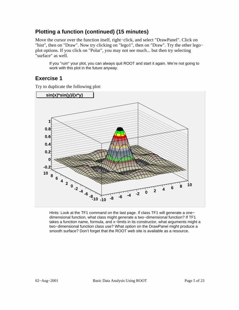
Exercise 1Try to duplicate the following plot:

-10 -8 -6 -4 -2 0 2 4 6 8 10

-10-8

-6-4

-20

24

68

10-0.2

0

0.2

0.4

0.6

0.8

1

sin(x)*sin(y)/(x*y)

Hints: Look at the TF1 command on the last page. If class TF1 will generate a one−dimensional function, what class might generate a two−dimensional function? If TF1takes a function name, formula, and x−limits in its constructor, what arguments might atwo−dimensional function class use? What option on the DrawPanel might produce asmooth surface? Don’t forget that the ROOT web site is available as a resource.


Working with Histograms (15 minutes)Histograms are described in Chapter 3 of the ROOT Users Guide. You may want to lookover this chapter later to get an idea of what else can be done with histograms otherthan what I cover in this class.

Let’s create a simple histogram:

[] TH1F h1("hist1","Histogram from a gaussian",100,−3,3)

Let’s look at what these arguments mean for a moment (and you should also look at thedescription of TH1F on the ROOT web site). The name of the histogram is "hist1". Thetitle displayed when plotting the histogram is "Histogram from a gaussian". There are100 bins in the histogram. The limits of the histogram are from −3 to 3.

Question: What should be the width of one bin of this histogram? Type the following tosee if your answer is the same as ROOT thinks it is:

[] h1.GetBinWidth(0)

Note that we have to indicate which bin’s width we want (bin 0 in this case), because youcan define histograms with varying bin widths.

If you type

[] h1.Draw()

right now, you won’t see much. That’s because the histogram is empty. Let’s randomlygenerate 10,000 values according to a distribution and fill the histogram with them:

[] h1.FillRandom("gaus",10000)

[] h1.Draw()

The "gaus" function is pre−defined by ROOT (see the TFormula class on the ROOT website; there’s also more on the next page of this tutorial). The default Gaussian distributionhas a width of 1 and a mean of zero.

Note the histogram statistics in the top right−hand corner of the plot. Question (for thosewho’ve had statistics): Why isn’t the mean exactly 0, or the width exactly 1?

Add another 10,000 events to histogram h1 with the FillRandom method (hit the up−arrows until you see "h1.FillRandom("gaus",10000)" again, and hit return). Click on thecanvas. Note how the histogram updates immediately, without another "Draw" command.

Move the mouse over the line of the histogram; note that it changes into an arrow insteadof a pointing finger. Right−click on the histogram and select "DrawPanel". Click on "E1:error/edges", then on "Draw".

The size of the error bars is equal to the square root of the number of events in thathistogram bin. With the up−arrow key in the ROOT command window, execute theFillRandom method a few more times and click on the histogram again. Question: Whydo the error bars get smaller?

You will often want to draw histograms with error bars. For future reference, you couldhave used the following command instead of the DrawPanel:

[] h1.Draw("e1")


Working with Histograms (continued) (15 minutes)Right−click on the histogram and select "SetMarkerAttributes" (at the bottom of themenu). Click on the solid square, click on the blue tile, then click on "Apply". If you clickon one of the circles on the bottom third of the panel and then click "Apply", you’llchange the size of the markers; try it.

Let’s create a function of our own:

[] TF1 myfunc("myfunc","gaus",0,3)

The "gaus" (or gaussian) function is actually

P0eB0.5

xBP1

P2

2

where P0, P1, and P2 are "parameters" of the function.• Let’s set these three parameters tovalues that we choose, draw the result, then create a new histogram from our function:

[] myfunc.SetParameters(10.,1.0,0.5)

[] myfunc.Draw()

[] TH1F h2("hist2","Histogram from my function",100,−3,3)

[] h2.FillRandom("myfunc",10000)

[] h2.Draw()

Note that we could also set the function’s parameters individually:

[] myfunc.SetParameter(1,−1.0)

[] h2.FillRandom("myfunc",10000)

• Optional note for advanced users:

In ROOT’s TFormula notation, this would be "[0]*exp(−0.5*((x−[1])/[2])^2)"; "[n]"corresponds to Pn. I mention this so that when you become more experienced withdefining your own parameterized functions, you can use a different formula:

[] TF1 myGaus("user", "[0]*exp(−.5*((x−[1])/[2])^2)/([2]*sqrt(2.*pi))")

This may seem cryptic to you now. Actually, it’s just a gaussian distribution with adifferent normalization so that P0 divided by the bin width becomes the number of eventsin the histogram:

[] myGaus.SetParameters(10.,0.,1.)

[] hist.Fit("user")

[] Double_t numberEquivalentEvents = myGaus.GetParameter(0) / hist.GetBinWidth(0)


Working with muliple plots (optional) (5 minutes)If you’re running short on time, you can skip this page (or any of the other optionalpages).

We have a lot of different histograms and functions now, but we’re plotting them all onthe same canvas, so we can’t see more than one at a time. There are two ways to getaround this.

First, we can create a new canvas by selecting "New Canvas" from the File menu of ourexisting canvas; this will create a new canvas with a name like "c1_n2". Try this now.

Second, we can divide a canvas into "pads". On the new canvas, right−click in the middleand select "Divide". Enter nx=2, ny=3, and click "OK".

Click on the different pads and canvases with the middle button. Observe how the yellowhighlight moves from box to box. The "target" of the Draw() method will be thehighlighted box. Try it: select one pad with the middle button, then enter

[] h2.Draw()

Select another pad or canvas with the middle button, and type:

[] myfunc.Draw()

At this point you may wish that you had a bigger monitor!


Saving and printing your work (15 minutes)By now you’ve probably noticed the "Save As" options under the "File" menu on thecanvas. What do all these options mean?

� "Save as canvas.ps" will create a Postscript file named <canvas−name>.ps; forexample, if you use this option from canvas c1, it will create "c1.ps". The image itcreates will be sized to fit an entire page.

� "Save as canvas.eps" will create an Encapsulated Postscript file. This file is suitablefor embedding into larger documents such as those created by LaTex, StarOffice, andMS−Word. Note that ROOT does not create an image preview; the Linux command"ps2epsi" can do this for you.

� "Save as canvas.gif" will create a GIF image, suitable for embedding into web pages.

� "Save as canvas.C" will create a file with the ROOT commands necessary to re−createthis canvas; more on this below.

� "Save as canvas.root" will create a native ROOT file with all the objects necessary tore−create this canvas; more on this below.

Select "Save as canvas.C" from one of the canvases in your ROOT session (the morecomplex the better). Let’s assume for the moment that the file "c1.C" is created. In yourUNIX window, type

> less c1.C

As you can see, this can be an interesting way to learn more ROOT commands. However,it doesn’t record the procedure you went through to create your plots, only the minimalcommands necessary to display them.

Next, select "Save as canvas.ps" from the same canvas; we’ll print it later.

Finally, select "Save as canvas.root" from the same canvas. Let’s assume the file is named"c1.root". Now quit ROOT with the ".q" command, and start it again.

To re−create your canvas from the ".C" file, use the command

[] .x c1.C

This is your first experience with a ROOT "macro", a stored sequence of ROOTcommands that you can execute at a later time. One advantage of the ".C" method is thatyou can edit the macro file, or cut−and−paste useful command sequences into macro filesof your own.

Quit ROOT and print out your Postscript file with the command

> qpr −Pqms1 c1.ps

This may be point at which you’ll notice that the default background color for ROOTplots is not pure white. You can change the background by right−clicking on a canvas andselecting "SetFillAttributes"; you’ll have to do this in the regions both outside and insidethe plot.


The ROOT browser (5 minutes)The ROOT browser is a useful tool, and you may find yourself creating one at everyROOT session. Read pages 25−26 of the ROOT Users Guide to find out how to makeROOT start a new browser automatically each time you start ROOT.

One way to retrieve the contents of file "c1.root" is to use the ROOT browser. Start upROOT and create a browser with the command:

[] TBrowser tb

In the right−hand pane, double−click on the folder with the same name as your homedirectory. Scroll through the list of files. You’ll notice special icons for any files that endin ".C" or ".root". If you double−click on a file that ends in ".C", ROOT will assume thefile contains a ROOT macro and interpret the contents. Try this on "c1.C", then close thecanvas window.

Now double−click on "c1.root". Nothing will appear to change. Now click on the "ROOTFiles" folder in the left−hand pane; this is the list of files currently opened by ROOT.Double−click on "c1.root" in the right−hand pane, then double−click on "c1;1".

What does "c1;1" mean? You’re allowed to write more than one object with the samename to a ROOT file (this topic is part of an optional lesson later in this class). The firstobject has ";1" put after its name, the second ";2", and so on. You can use this facility tokeep many versions of a histogram in a file, and be able to refer back to any previousversion.

At this point, saving a canvas as a ".C" file or as a ".root" file may look the same to you.But these files can do more than save and re−create canvases. In general, a ".C" file willcontain ROOT commands and functions that you’ll write yourself; ".root" files will containcomplex objects such as n−tuples.


Fitting a histogram (15 minutes)

I created a file with a couple of histograms in it for you to play with. Switch to yourUNIX window and copy this file into your directory:

> cp ~seligman/root−class/histogram.root $cwd

Go back to your browser window. (If you’ve quit ROOT, just start it again and start anew browser.) Click on the folder in the left−hand pane with the same name as your homedirectory. If you don’t see "histogram.root", select "Refresh" from the "View" menu.

Double−click on "histogram.root", click on "ROOT Files" in the left−hand pane, thendouble−click on "histogram.root" in the right−hand pane. You can see that I’ve createdtwo histograms with the names "hist1" and "hist2". Double−click on "hist1".

You can guess from the x−axis label that I created this histogram from a gaussiandistribution, but what were the parameters? In physics, to answer this question wetypically perform a "fit" on the histogram: you assume a functional form that depends onone or more parameters, and then try to find the value of those parameters that makethe function best fit the histogram.

Right−click on the histogram and select "FitPanel". Click on "gaus", then click on "Fit".You’ll see two changes: A function is drawn on top of the histogram, and the fit resultsare printed on the ROOT command window.

Interpreting fit results takes a bit of practice. Recall that a gaussian has 3 parameters(P0, P1, and P2); these are labeled "Constant", "Mean", and "Sigma" on the fit output.ROOT determined that the best value for the "Mean" was 5.96±0.03, and the best valuefor the "Sigma" was 2.47±0.02. Compare this with the Mean and RMS printed in the boxon the upper right−hand corner of the histogram. Statistics questions: Why are thesevalues almost the same as the results from the fit? Why aren’t they identical?

On the canvas, select "Show Fit Parameters" from the "Options" menu. Click on "Fit" onthe FitPanel again. Just as a check, click on "landau" on the FitPanel and click on "Fit"again; then click on "expo" and fit again.

It looks like of the three choices (gaussian, landau, exponential), the gaussian is the bestfunctional form for this histogram. Take a look at the "Chi2 / ndf" value in the statisticsbox on the histogram ("Chi2 / ndf" is pronounced "kie−squared per degrees of freedom").Do the fits again, and observe how this number changes. Typically, you know you havea good fit if this ratio is about 1.


Fitting a histogram (continued) (15 minutes)

Go back to the browser window and double−click on "hist2". Uh−oh; this doesn’t looklike a gaussian. Right−click on the histogram and select "FitPanel" (be careful not to re−use the FitPanel from "hist1"). Click on "gaus" and then on "Fit". Uggh −− that’s aterrible fit! You can try the landau and exponential functions, but they won’t work muchbetter.

You’ve probably already guessed by reading the x−axis label that I created thishistogram from the sum of two gaussian distributions. But you’ve probably also noticed abutton on the FitPanel labeled "user"; this is for fitting to a user−defined function.

In order to use this button, you have to define a function that has the name "user".

Define a user function with the following command:

[] TF1 func("user","gaus(0)+gaus(3)")

Note that the internal ROOT name of the function has to be "user", but not the functionobject itself.

What does "gaus(0)+gaus(3)" mean? You already know that the "gaus" function usesthree parameters. "gaus(0)" means to use the gaussian distribution starting withparameter 0; "gaus(3)" means to use the gaussian distribution starting with parameter 3.This means our user function has six parameters: P0, P1, and P2 are the "constant","mean", and "sigma" of the first gaussian, and P3, P4, and P5 are the "constant", "mean",and "sigma" of the second gaussian.

Now try to do a fit by going to the FitPanel, clicking on "user", then clicking on "Fit".

If you look at the ROOT command window, you’ll see that all six parameters have thevalue "nan", which means "Not A Number." For all but the simplest fits, ROOT needs tohave some starting values for its fit parameters.

Let’s set the values of P0, P1, P2, P3, P4, and P5:

[] func.SetParameters(5.,5.,1.,1.,10.,1.)

Then click on "Fit" on the FitPanel.

The results are not much better. This is because I deliberately picked a poor set ofstarting values. Let’s try a better set:


These starting values don’t look much different, but try to fit the histogram again.

These simple fit examples may leave you with the impression that all histograms inphysics are fit with gaussian distributions. Nothing could be further from the truth. I’musing gaussians in this class because they have properties (mean and width) that youcan determine by eye.

Chapter 5 of the ROOT Users Guide has a lot more information on fitting histograms,and a much more realistic example.

If you want to see how I created the file histogram.root, go to the UNIX window and type:

> less ~seligman/root−class/CreateHist.C


Saving your work, part 2 (optional) (15 minutes)

So now you’ve got a histogram fitted to a complicated function. Try "Save as canvas.C"from the "File" menu, and examine the result in your UNIX window with

> less c1.C

I know it looks like a bunch of C++ commands. But if you look carefully, you’ll see thatthe user function you just created is not re−created in the macro.

If you were to use "Save as canvas.root", quit ROOT, restart it, then load canvas "c1;1"from the file, you’d get your histogram back with the function superimposed... but it’s notobvious where the function is or how to access it now.

What if you want to save your work in the same file as the histograms you just read in?You can do it, but not by using the ROOT browser. The browser will only open files inread−only mode. To be able to modify a file, you have to open it with ROOT commands.

Try the following: Quit ROOT (note that you can select "Quit ROOT" from the "File"menu of the canvas or the browser). Start ROOT again, then modify "histogram.root"with the following commands:

[] TFile file1("histogram.root","UPDATE")

It is the "UPDATE" option that will allow you to write new objects to "histogram.root".

[] hist2.Draw()

For the following two commands, try hitting the up−arrow key until you see them again.ROOT stores the last 80 or so ROOT commands you’ve typed in the file ".root−hist" inyour home directory, and let’s you re−use them with the arrow keys.

[] TF1 func("user","gaus(0)+gaus(3)")


The following command is the same as clicking on "user" and "Fit" on the FitPanel:

[] hist2.Fit("user")

Now you can do what you couldn’t before: save objects into the ROOT file:

[] hist2.Write()

[] func.Write()

You should close the file to make sure you save your changes:

[] file1.Close()

Quit ROOT, start it again, and use the ROOT browser to open "histogram.root". You’llsee a couple of new objects: "hist2;2" and "user;1". Double−click on each of them to seewhat you’ve saved.

Chapter 9 of the ROOT Users Guide has more information on using ROOT files.


Dealing with PAW files (optional) (5 minutes)Suppose someone gives you a file that contains n−tuples or histograms that werecreated with PAW, HBOOK, or CERNLIB (actually, to first order these are three differentnames for the same thing). How do you read these files using ROOT?

The answer is that you can’t, at least not directly. You must convert these files intoROOT format using the command "h2root".

For example, if someone gives you a file called "testbeam.hbook", you can convert it withthe command

> h2root testbeam.hbook

This creates a file "testbeam.root" that you can open in the ROOT browser.

There is no simple way of converting a ROOT file back into PAW/HBOOK/CERNLIBformat. You generally have to write a custom program with both FORTRAN and C++subroutines to accomplish this task.

Note that the "h2root" command is set up (along with ROOT) with the command

> setup root

that you type when you log in. If you accidentally type "h2root" (or "root") before you setup ROOT, you’ll get the error message:

h2root: Command not found

You can get more information about "h2root" by using a special form of the "man"command:

> man $ROOTSYS/man/h2root.1


Accessing variables in ROOT NTuples/Trees (15 minutes)I’ve created a sample ROOT n−tuple in ~seligman/root−class/tree.root.

Start fresh by quitting ROOT. Copy my 2.1 MB example tree file with the command

> cp ~seligman/root−class/tree.root $cwd

Start ROOT again. Start a new browser with the command

[] TBrowser b

Click on the folder in the left−hand pane with the same name as your home directory.Double−click on "tree.root", click on "ROOT Files" in the left−hand pane, then double−click on "tree.root" in the right−hand pane. There’s just one object inside: "tree1", aROOT tree (or n−tuple) with 100,000 simulated physics events.

Actually, there’s little or no real physics associated with the contents of this tree. Icreated it solely to illustrate ROOT concepts, not to demonstrate real physics with a realdetector.

Right−click on the "tree1" icon, and select "StartViewer". You’re looking at aTreeViewer, an interface to help you analyze ROOT trees. Focus on the second column inthe right−hand pane of the TreeViewer; these are the variables stored in the tree.

In this overly−simple example, an imaginary particle is travelling in a positive directionalong the z−axis with energy "ebeam". It hits a target at z=0, and travels a distance "zv"before it is deflected by the material of the target. The particle’s new trajectory isrepresented by "px", "py", and "pz", the final momenta in the x−, y−, and z−directionsrespectively. The variable "chi2" represents a confidence level in the measurement ofthe particle’s momentum.

Did you notice what’s missing from the above description? One important thing that’smissing is the units; for example, I didn’t tell you whether "zv" is in millimeters,centimeters, inches, yards, etc. Such information is not usually stored inside an n−tuple;you have to find out what it is and include the units in the labels of the plots you create.For this example, assume that "zv" is in centimeters (cm), and all energies and momentaare in GeV.

Double−click on the names of the variables and see what happens.

There is a "Help" menu on the upper right−hand side of the TreeViewer menu. Unlike theHelp menus on the browser and canvas menu, which are only marginally informative,the Help offered on the TreeViewer is genuinely useful.

By the way, the variable "event" is just the event number (it’s 0 for the first event, 1 forthe second event, 2 for the third event... 99999 for the 100,000th event).


Correlating variables: scatterplots and expressions (15 minutes)Left−click on a variable and hold the mouse down. Drag the variable next to the bluecurly "X" in the first column, over the word "−empty−", and let go of the button. Nowselect a different variable and drag it over next to the curly "Y". Click on the scatterploticon in the lower left−hand corner of the TreeViewer (it’s next to a button labeled"STOP", you may have to move the TreeViewer window).

This is a scatterplot, a handy way of observing the correlations between two variables.Be careful: it’s easy to fall into the trap of thinking that each (x,y) point on a scatterplotrepresents two values in your n−tuple. In fact, the scatterplot is a grid and each square inthe grid is randomly populated with a density of dots that’s proportional to the number ofvalues in that grid.

Drag different pairs of variables to the "X" and "Y" boxes and look at the scatterplots. Doyou see any correlations between the variables?

If you just see a shapeless blob on the scatterplot, the variables are likely to beuncorrelated; for example, plot "px" versus "py". If you see a pattern, there may be acorrelation; for example, plot "pz" versus "zv". It appears that the higher "pz" is, the lower"zv" is, and vice versa. Perhaps the particle loses energy before it is deflected in thetarget.

You can also create expressions that are functions of the variables in the tree. Double−click on one the "E()" icons that has the word "−empty−" next to it. In the dialog box,type "sqrt(px*px+py*py)" in the box under "Expression", and type "pt" in the box under"Alias". Then click on "Done". Now double−click on the word "~pt" in the TreeViewer.

When you’re typing in the expression, you don’t have to type the name of any variable inthe tree. You can just click on the name in the TreeViewer. By the way, "pt" is thetransverse momentum of the particle, that is, the component of the particle’s momentumthat’s perpendicular to the z−axis.

Let’s do this again to calculate theta, the angle the particle makes with the z−axis.Double−click on a different "E()" icon with "−empty−" next to it. Type "atan(~pt/pz)"under "Expression", and "theta" under "Alias". Click "Done", then double−click on"~theta".

After an expression is no longer empty, you can’t double−click on it to edit it; that will justcause the expression to be plotted. To edit an existing expression, right−click on it andselect "EditExpression."

Note that you can have expressions within expressions (such as "~pt" in the definition of"~theta". All expressions that you create must have names that begin with a tilde (~), andthe expression editor will enforce this. A common error is to forget the tilde when you’retyping in an expression; that’s the reason why it can be a good idea to insert a variableor an alias into an expression by clicking on it in the TreeViewer.

By the way, the units of theta in this example are radians.


Correlating variables: cuts (15 minutes)

Let’s create a "cut" (a limit on the range of a variable to be plotted). Edit another emptyexpression and give it the formula "zv < 20" and the alias "zcut".

Note how the icon changes in the TreeViewer. ROOT recognizes that you’ve typed alogical expression instead of a calculation.

Drag "~zcut" to the scissor icon. Double−click on "zv" to plot it. Double−click on someof the other variables and look at the "Nent" in the statistics box of the histograms; the z−cut affects all the plots, not just the plot of "zv".

Double−click on the scissor icon to turn off the cut; note the change in the scissor icon.Double−click on the icon again to turn the cut back on.

Now edit "~zcut" by right−clicking on it and selecting "EditExpression". Edit theexpression to read "zv<20 && zv>10" and click "Done." Plot "zv". Has the cut changed?Now drag "~zcut" to the scissors and plot "zv" again.

A note for advanced users: A "cut" is actually a weight that ROOT applies when filling ahistogram; a logical expression has the value 1 if true and the value 0 if false. If you wantto fill a histogram with weighted values, use an expression for the cut that correspondsto the weight. For example, a cut of "1/e" will fill a histogram with each event weighted by1/e; a cut of "(1/e)*(sqrt(z)>3.2)" will fill a histogram with events weighted by 1/e, forthose events with sqrt(z) greater than 3.2.

In a complex analysis, you may have large number of expressions and cuts in yourTreeViewer. You can save them so you don’t have to type them all again. From the "File"menu, select "Save source". ROOT will create a file named "treeviewer.C".

If you want to look at the results, switch to your UNIX window and type:

> less treeviewer.C

Quit ROOT and start it again. Type

[] .x treeviewer.C

ROOT will open the tree file for you, and set up the TreeViewer with the sameexpressions and cuts.

If you are analyzing more than one tree, you may want to save multiple TreeViewers. Asimple way to do this is to rename the treeviewer.C file after you save it. The UNIXcommand to rename a file is "mv"; for example:

> mv treeviewer.C dileptonviewer.C

If you did this, you’d have to edit dipleptonviewer.C and change the the top line from

void treeviewer() {

to

void dileptonviewer() {

That is, the name of the .C file and the name of the viewer function must match.


A simple analysis example (15 minutes)Let’s walk through a simple example of what can be done with the tools you’ve learnedso far. An actual physics analysis is much more complex, but this may give you a "feel"for what’s involved.

Make a histogram of "chi2".

There’s a peak around 1, but the x−axis extends far beyond that, up to chi2 > 18.Evidentally there are some events with a large chi2, but not enough of them to show upon the plot.

Make a scatterplot of "chi2" versus "ebeam".

On the scatterplot, we can see a dark band that represents the main peak of the chi2distribution, and a scattering of dots that represents a group of events with anomalouslyhigh chi2.

The chi2 represents a confidence level in reconstructing the particle’s trajectory. If thethe chi2 is high, the trajectory reconstruction was poor. It would be perfectly acceptableto apply a cut of "chi2 < 1.5", but let’s see if we can correlate a large chi2 with anythingelse.

Make scatterplots of "chi2" versus the other variables, including the expressions. Doesanything stand out?

Take a careful look at "chi2" vs. "~theta". It looks like all the large−chi2 values are foundin the region theta > 0.15 radians. It may be that our trajectory−finding code has aproblem with large angles. Let’s put in both a theta cut and a chi2 cut to be certain we’relooking at a sample of events with good reconstructed trajectories.

Create a new cut "~cutChi2" with an expression of "chi2 < 1.5". Create another new cut"~cutTheta" with an expression of "~theta < 0.15". Now create a third cut "~cutAll" withan expression of "~cutChi2 && ~cutTheta". Drag "~cutAll" to the scissor icon and plot"chi2".

There’s nothing wrong with just creating one cut "chi2 < 1.5 && ~theta < 0.15", but Iwanted to illustrate that you can combine cut expressions in the same way that you cancombine any other expression.

I must confess: I cheated when I pointed you directly to theta as the cause of the chi2problem. I knew this because I wrote the program that created the tree. If you want tolook at this program youself, go to the UNIX window and type:

> less ~seligman/root−class/CreateTree.C

By the way, you’ve made a lot of plots, but you’ve probably only looked at them one at atime. Don’t forget that you can view multiple plots in a couple of ways: You can select"New canvas" from the "File" menus of the browser, any canvas, or the TreeViewer. Youcan select one canvas, right−click on it, select "Divide", and enter the number ofhorizontal and vertical divisions; don’t forget to use the middle button to select the pad orcanvas you wish to draw to.

There is a much more detailed description of trees and how to analyze them in Chapter10 of the Users Guide.


A technical problem (optional) (10 minutes)

Make a histogram of "zv". That looks like an exponential distribution; let’s try to do a fit.Right−click on the histogram, select "FitPanel", click on "expo", then on "Fit".

The ROOT command window displays the result of the fit, but no function wassuperimposed on the histogram. What happened?

By default, when you make a plot using the TreeViewer, it’s written to a histogramnamed "htemp". You can see this name in the TreeViewer; it’s in the "Histogram" field inthe status bar just below the menu bar.

"htemp" is a handy storage area for histograms, but it has a couple of problems: it getsoverwritten all the time, and it has some simplifying properties. Among those simpleproperties is that you cannot store or display an associated function with the histogram.

What you can do is create a new histogram with whatever properties you like.

In the "Histogram" field of the TreeViewer, type a new name ("zhist", for example).Double−click on "zv" to make a histogram; this time a new histogram named "zhist" willbe created. Right−click on the new histogram, select the FitPanel, and fit to anexponential distribution.

Now, before you do anything else: double−click on "chi2".

Oops −− neither the x−axis nor the plot labels changed. Your new histogram "zhist" isnot the same thing as ROOT’s "htemp". If you supply a new histogram via theTreeViewer, you must remember to change it back to "htemp" or a different histogrambefore making new plots.

By the way, you don’t have to let the TreeViewer create the histogram for you. If youwant to specify the properties of the histogram yourself (for example, the bin limits), youcan create the histogram using a ROOT command; for example:

[] TH1F zh1("zhist","z vertex distribution",100,10.,20.)

and then put "zhist" in the TreeViewer.


Analysis Macros (optional) (15 minutes)The TreeViewer can get you started, but it’s not enough for serious data analysis. Atsome point, you need to leave the graphic user interface behind and start working withROOT macros.

ROOT makes the procedure relatively painless, but it’s still a bit complex for thebeginning student. The following section is for both you and your supervisor. Typically,your supervisor will prepare the ROOT/C++ code for you; all you have to do is run it andmake occasional changes.

The first step to have ROOT write the skeleton of an analysis class for you. This is donewith MakeClass. This example assumes you’re still working with my "tree1" example.

If you don’t already have the ROOT tree open, open it with the following command:

[] TFile myFile("tree.root")

Now create an analysis macro for "tree1" with MakeClass:

[] tree1.MakeClass("Analyze")

Switch to the UNIX window and examine the files that were created:

> less Analyze.h

> less Analyze.C

Unless you’re familiar with C++, this probably looks like gobbledy−gook to you. (I knowC++, and it looks like gobbledy−gook to me.) Fortunately, there are only two routinesthat should be modified: Loop and possibly Cut.

As an example, I’ve prepared two files for someone familiar with C++ to compare withthe code that MakeClass generates. You can see the differences with the commands:

> diff Analyze.h ~seligman/root−class/AnalyzeExample.h

> diff Analyze.C ~seligman/root−class/AnalyzeExample.C

What is the point of this? By itself, the class "Analyze" that you created does nothing.The "AnalyzeExample" files I created contain a revised version of Analyze that doessomething. By comparing an analysis macro that does nothing with one that doessomething, you can get an idea of how to revise a macro yourself.

Remember, unless two trees happen to have exactly the same variables, an analysismacro that you create for one tree will not be the same as that for any other. You mayhave to edit an analysis macro for each tree you work with.


Analysis Macros continued (optional) (10 minutes)After an analysis class has been prepared, you use it by loading it into ROOT, creatingan object of that class, and invoking its Loop() method. The class will open the tree filefor you if it’s not already open.

Try this: copy my example into your directory with

> cp ~seligman/root−class/AnalyzeExample.* $cwd

Quit ROOT, start it again, and enter the following lines:

[] .L AnalyzeExample.C

[] Analyze a

[] a.Loop()

It may help to remember that while the names of my files begin with "AnalyzeExample",the name of the class defined in those files is still just "Analyze".

If you make any changes to an analysis macro, you have to load it again with ".L".


Exercise 2 (optional, for those willing to work with C++)This exercise is not as hard as it looks at first. It only requires you to duplicate someexisting lines in AnalyzeExample.C and make small changes to them. To helpunderstand the C++ commands in AnalyzeExample.C, it may help to read "Classes,Methods and Constructors" on page 16 of the ROOT Users Guide.

The code in AnalyzeExample.C makes a histogram of the variable "zv". Revise the codeso that it also makes a histogram of the variable "chi2".

Hints:

� There are typically three things you have to do with histograms in a program: definethem (the slang for this is "book them"), fill them, and print or draw them.

� The range of values of the "chi2" variable in "tree.root" is not the same as the rangeof values of "zv".

� In C++, every statement must end with a semicolon (;).

Exercise 3 (optional, for those willing to work with C++)

Assuming a relativistic particle, the measured energy of the particle is given by

Emeas

2 =Px

2+Py

2+Pz

2

and the energy lost by the particle is given by

Eloss=E

beamBE

meas

Revise AnalyzeExample.C to also make a scatterplot of Eloss vs. "zv". Is there a

relationship between the z−distance travelled in the target and the amount of energy lost?

Exercise 4 (optional, for those willing to work with C++)OK, enough with the kid gloves. Here’s one that may make you sweat a little.

Right now, AnalyzeExample.C is drawing the histograms at the end of its Loopprocedure. Revise the program so that it does not draw the histograms on the screen, butwrites them to a file instead. No, you don’t want to write the histograms to "tree.root";write them to a different file named "analysis−example.root". Don’t forget to label theaxes of your plots! When you’re done, open "analysis−example.root" in ROOT and checkthat your plots are what you expect.

Hints:

� You’ve created a lot of ".C" files during the course of this tutorial. Some of them maycontain commands that will help you in this exercise.

� Don’t forget to use the ROOT web site as a reference. Here’s a question that’s also abit of a hint: What would be the difference between opening your new file with"UPDATE" access, "RECREATE" access, and "NEW" access? Why might it be a badidea to open a file with "NEW" access? (A hint within a hint: what would happen if youran your macro twice?)


Feynmann diagrams (optional)This page is meant for physicists who are going over these notes; it’s unlikely thatsummer students will have to worry about making Feynmann diagrams.

Let’s start fresh: quit ROOT and start it again. Create a new canvas with the command:

[] TCanvas diagram("diagram","Feynmann diagram")

Now select "Editor" from the "Edit" menu.

Most of the options are self−explanatory. For example, to create a line, click on the"Line" button in the Editor. Click on the canvas, hold the button down, and drag themouse to draw the line.

Once you’ve created a line or other graphical element, you can edit it... but it’s notalways clear where you have to click or drag the mouse. You have to carefully watchhow the shape of the cursor changes as you move it over your drawing. In particular,Ellipses and CurlyArcs can be tricky to work with; their "anchors" are located outside theellipse.

Try right−clicking on the shapes to see what drawing options you have. You can changea "curly" line (gluon−like) to a "wavy" line (photon−like) by right−clicking on it andselecting "SetWavy".

For text, click on the "Text/Latex" button, then click on the canvas where you’d like thetext to go. The cursor will change into a question mark. Type your text, then hit the enterkey. Try entering the text "q_{1}" and see what happens; ROOT contains a subset ofLatex. For more information, see the section on "Text and Latex MathematicalExpressions" in Chapter 8 of the Users Guide.

Once you’ve got your diagram, you should save it with "Save as canvas.root" or "Saveas canvas.C" under the "File" menu (so you can edit it later), and with "Save ascanvas.eps" (so you can include it in your article).


Documents

Basic Data Analysis Using ROOT - Nevis Laboratoriesseligman/root-class/Root...Basic Data Analysis Using ROOT A guide to this tutorial If you see a command in this tutorial is preceded