Embed Size (px)
Citation preview

Basic Data Mining Techniques
Chapter 3
3.1 Decision Trees
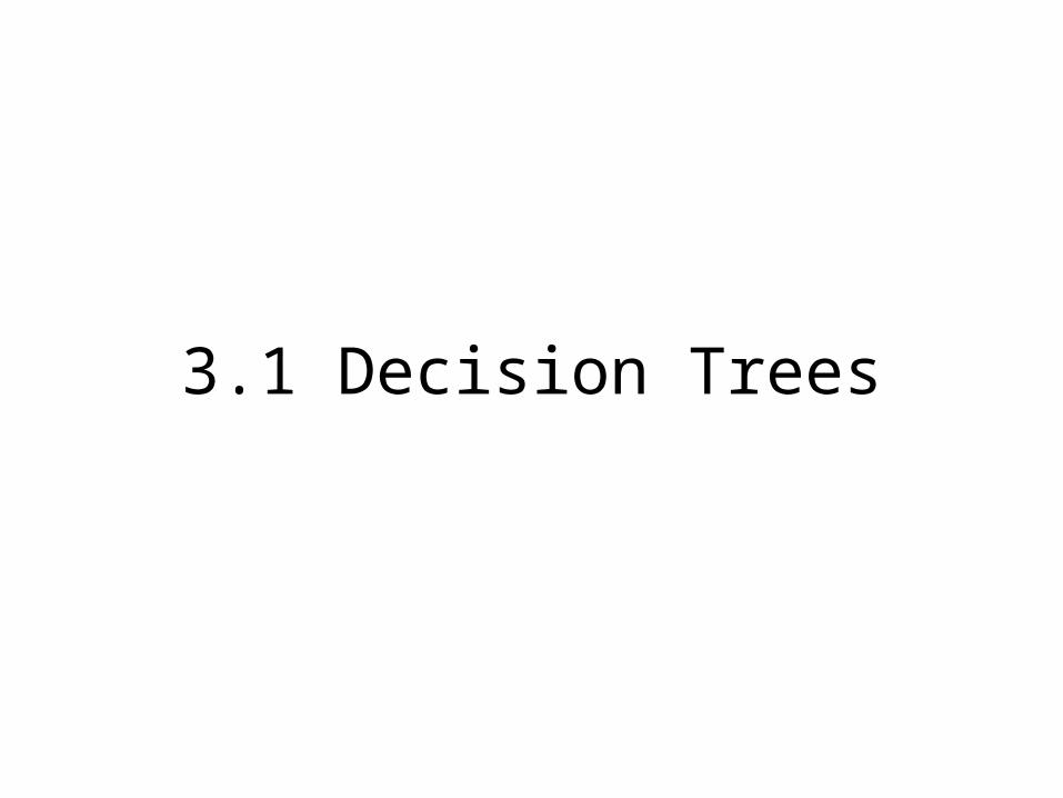
An Algorithm for Building Decision Trees
1. Let T be the set of training instances.2. Choose an attribute that best differentiates the instances in T.3. Create a tree node whose value is the chosen attribute.
-Create child links from this node where each link represents a unique value for the chosen attribute.-Use the child link values to further subdivide the instances into subclasses.
4. For each subclass created in step 3: -If the instances in the subclass satisfy predefined criteria or if the set of
remaining attribute choices for this path is null, specify the classification for new instances following this decision path. -If the subclass does not satisfy the criteria and there is at least one attribute to further subdivide the path of the tree, let T be the current set of subclass instances and return to step 2.
(i.e. accuracy)
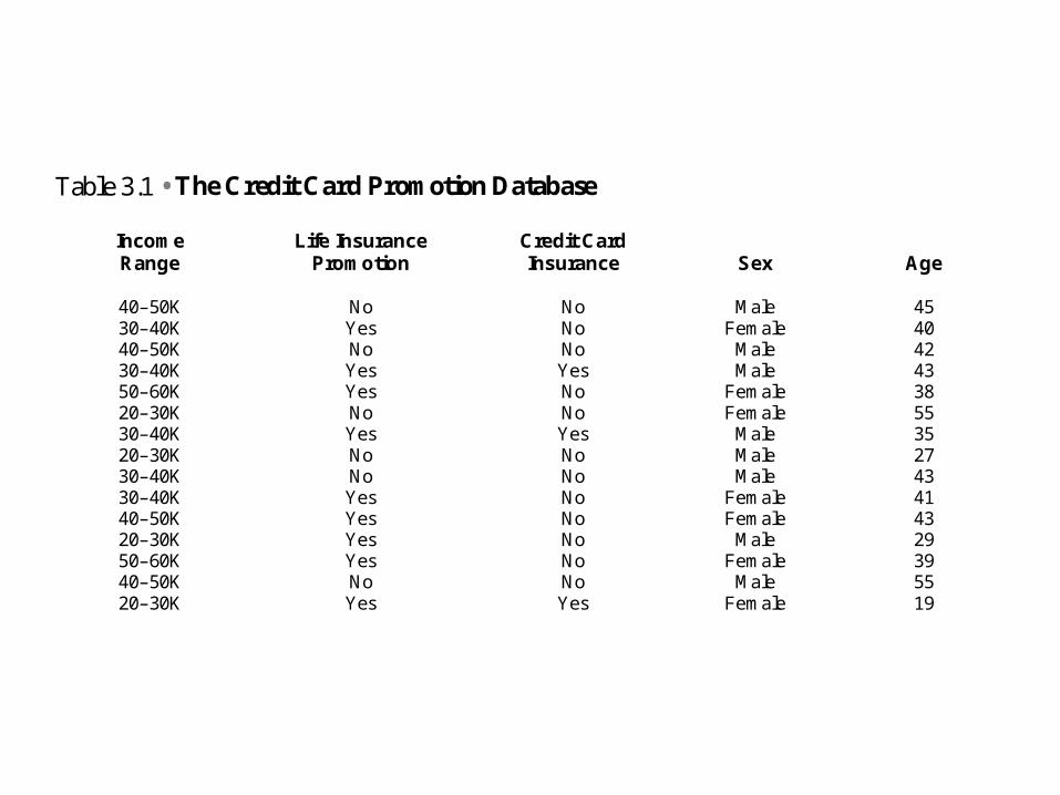
Table 3.1 • The Credit Card Promotion Database
Income Life Insurance Credit CardRange Promotion Insurance Sex Age
40–50K No No Male 4530–40K Yes No Female 4040–50K No No Male 4230–40K Yes Yes Male 4350–60K Yes No Female 3820–30K No No Female 5530–40K Yes Yes Male 3520–30K No No Male 2730–40K No No Male 4330–40K Yes No Female 4140–50K Yes No Female 4320–30K Yes No Male 2950–60K Yes No Female 3940–50K No No Male 5520–30K Yes Yes Female 19
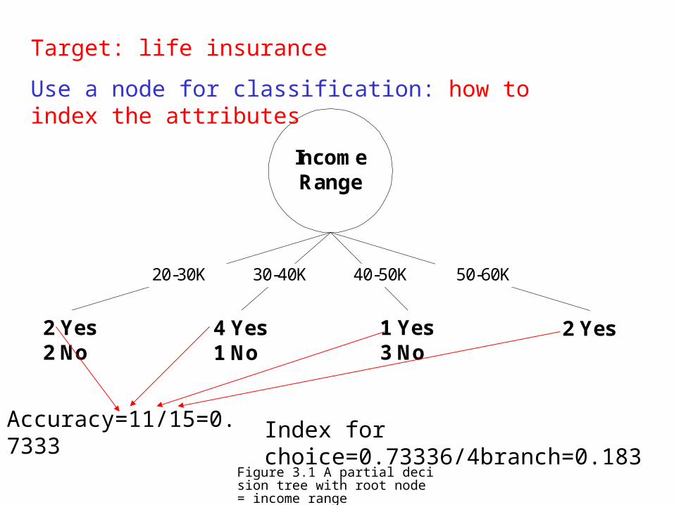
Figure 3.1 A partial decision tree with root node = income range
IncomeRange
30-40K
4 Yes1 No
2 Yes2 No
1 Yes3 No
2 Yes
50-60K40-50K20-30K
Target: life insurance
Use a node for classification: how to index the attributes
Accuracy=11/15=0.7333 Index for choice=0.73336/4branch=0.183
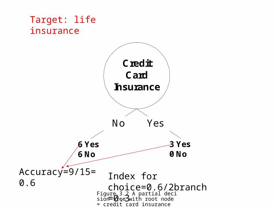
Figure 3.2 A partial decision tree with root node = credit card insurance
CreditCard
Insurance
No Yes
3 Yes0 No
6 Yes6 No
Target: life insurance
Accuracy=9/15=0.6 Index for choice=0.6/2branch=0.3
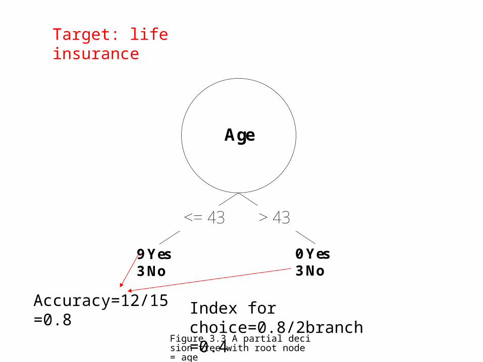
Figure 3.3 A partial decision tree with root node = age
Age
<= 43 > 43
0 Yes3 No
9 Yes3 No
Target: life insurance
Accuracy=12/15=0.8 Index for choice=0.8/2branch=0.4
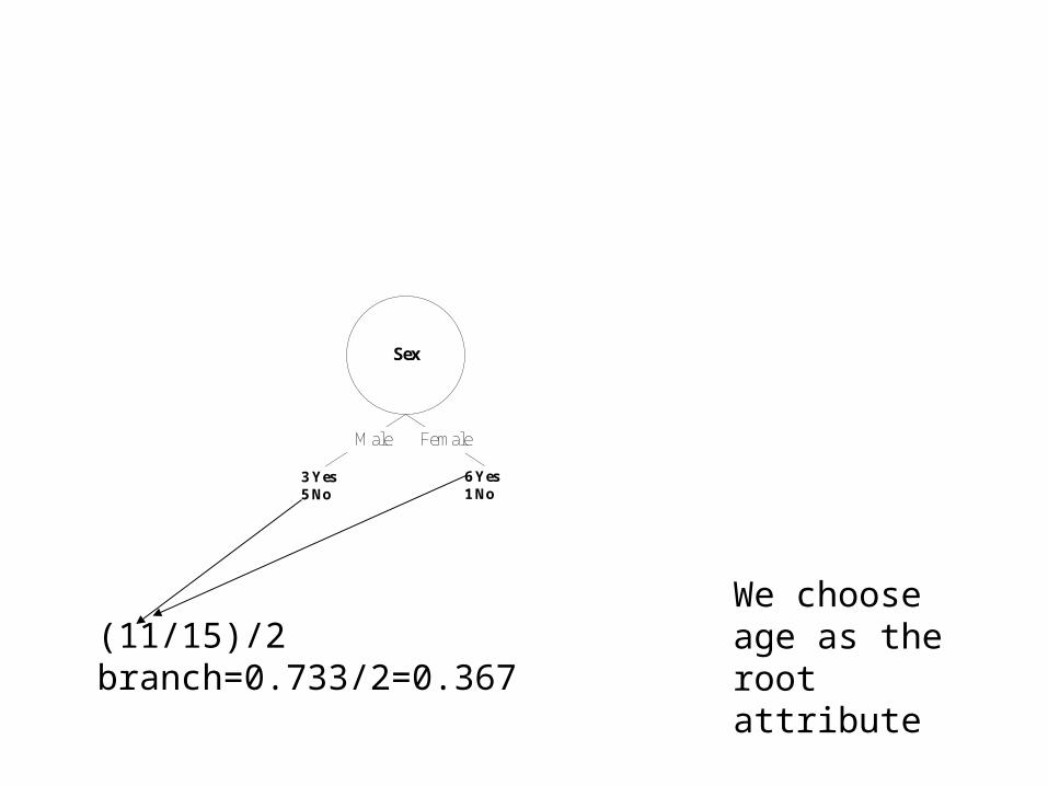
(11/15)/2 branch=0.733/2=0.367We choose age as the root attribute
Sex
Male Female
6 Yes1 No
3 Yes5 No

ID3
• See homework

Decision Trees for the Credit Card Promotion Database
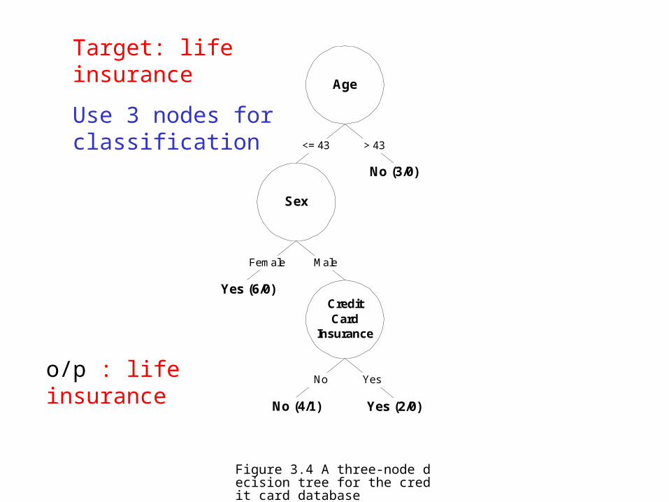
Figure 3.4 A three-node decision tree for the credit card database
Age
Sex
<= 43
Male
Yes (6/0)
Female
> 43
CreditCard
Insurance
YesNo
No (4/1) Yes (2/0)
No (3/0)
o/p : life insurance
Target: life insurance
Use 3 nodes for classification
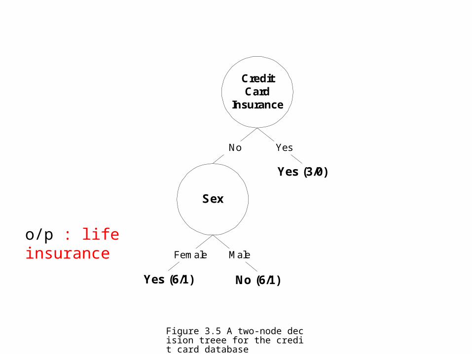
Figure 3.5 A two-node decision treee for the credit card database
CreditCard
Insurance
Sex
No
Male
Yes (6/1)
Female
Yes
Yes (3/0)
No (6/1)
o/p : life insurance
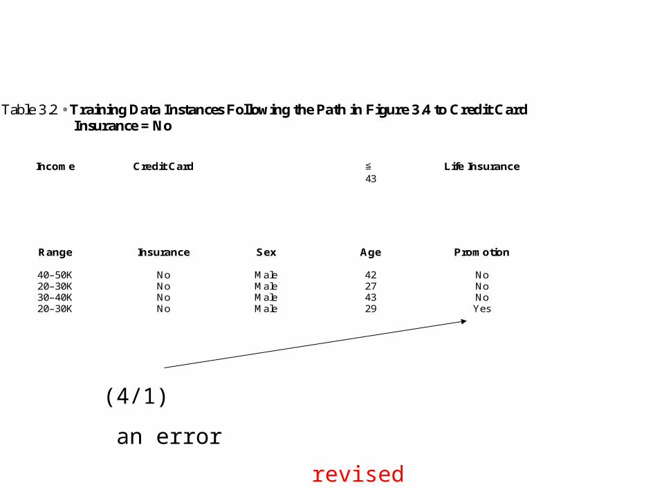
Table 3.2 • Training Data Instances Following the Path in Figure 3.4 to Credit Card Insurance = No
Income Credit Card ≦
43
Life Insurance
Range Insurance Sex Age Promotion
40–50K No Male 42 No 20–30K No Male 27 No 30–40K No Male 43 No 20–30K No Male 29 Yes
(4/1)
an error
revised
Decision Tree Rules
A Rule for the Tree in Figure 3.4
IF Age <=43 & Sex = Male & Credit Card Insurance = NoTHEN Life Insurance Promotion = No
A Simplified Rule Obtained by Removing Attribute Age
IF Sex = Male & Credit Card Insurance = No THEN Life Insurance Promotion = No
Other Methods for Building Decision Trees
• CART (Classification and Regression Tree)
• CHAID (Chi-Square Automatic Interaction Detector)
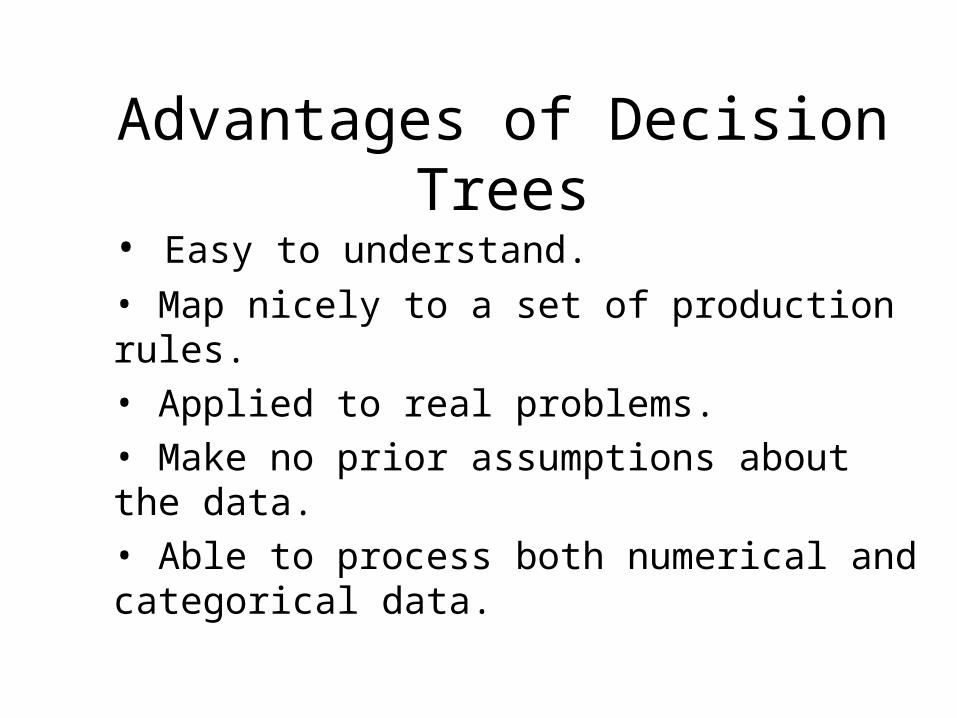
Advantages of Decision Trees
• Easy to understand.
• Map nicely to a set of production rules.• Applied to real problems.• Make no prior assumptions about the data.• Able to process both numerical and categorical data.
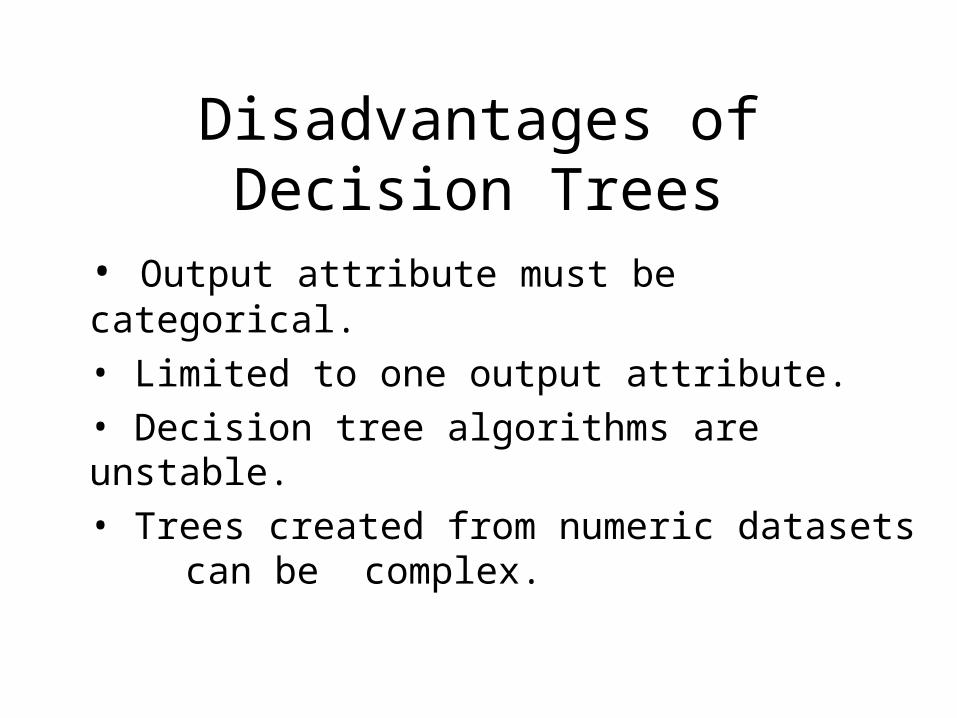
Disadvantages of Decision Trees
• Output attribute must be categorical.
• Limited to one output attribute.• Decision tree algorithms are unstable.• Trees created from numeric datasets can be complex.
3.2 Generating Association Rules

Confidence and Support
Rule Confidence
Given a rule of the form “If A then B”, rule confidence is the conditional probability that B is true when A is known to be true.
Rule Support
The minimum percentage of instances in the database that contain all items listed in a given association rule.
Mining Association Rules: An Example
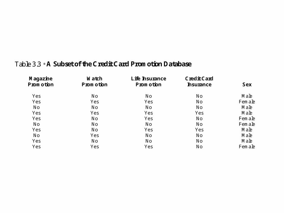
Table 3.3 • A Subset of the Credit Card Promotion Database
Magazine Watch Life Insurance Credit CardPromotion Promotion Promotion Insurance Sex
Yes No No No MaleYes Yes Yes No FemaleNo No No No MaleYes Yes Yes Yes MaleYes No Yes No FemaleNo No No No FemaleYes No Yes Yes MaleNo Yes No No MaleYes No No No MaleYes Yes Yes No Female
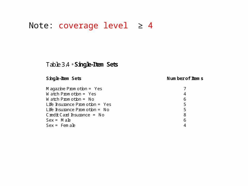
Table 3.4 • Single-Item Sets Single-Item Sets Number of Items Magazine Promotion = Yes 7 Watch Promotion = Yes 4 Watch Promotion = No 6 Life Insurance Promotion = Yes 5 Life Insurance Promotion = No 5 Credit Card Insurance = No 8 Sex = Male 6 Sex = Female 4
Note: coverage level ≥ 4
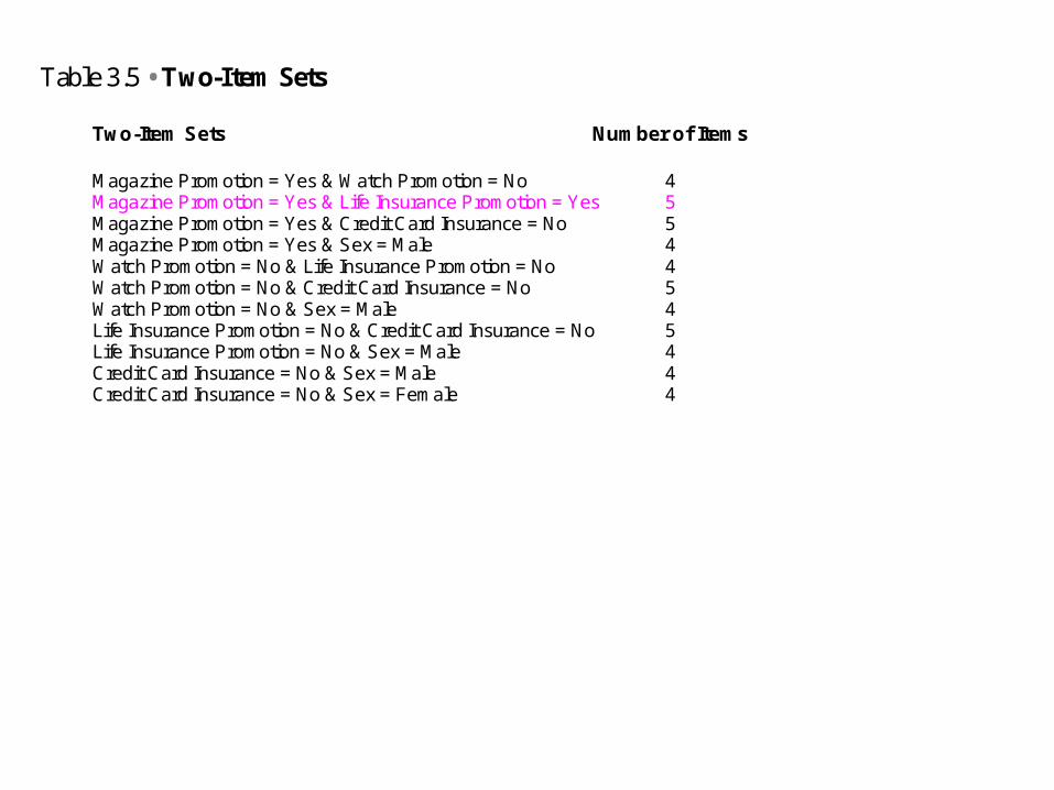
Table 3.5 • Two-Item Sets
Two-Item Sets Number of Items
Magazine Promotion = Yes & Watch Promotion = No 4 Magazine Promotion = Yes & Life Insurance Promotion = Yes 5 Magazine Promotion = Yes & Credit Card Insurance = No 5 Magazine Promotion = Yes & Sex = Male 4 Watch Promotion = No & Life Insurance Promotion = No 4 Watch Promotion = No & Credit Card Insurance = No 5 Watch Promotion = No & Sex = Male 4 Life Insurance Promotion = No & Credit Card Insurance = No 5 Life Insurance Promotion = No & Sex = Male 4 Credit Card Insurance = No & Sex = Male 4 Credit Card Insurance = No & Sex = Female 4
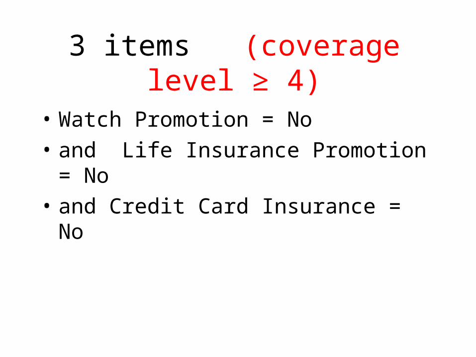
3 items (coverage level ≥ 4)
• Watch Promotion = No
• and Life Insurance Promotion = No
• and Credit Card Insurance = No
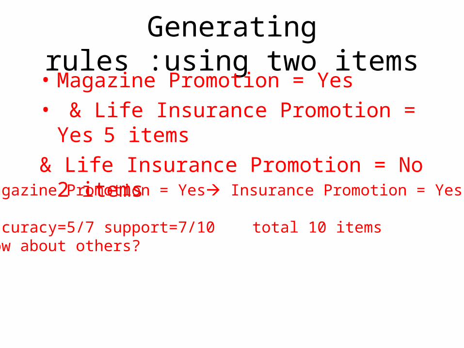
Generating rules :using two items• Magazine Promotion = Yes
• & Life Insurance Promotion = Yes 5 items
& Life Insurance Promotion = No 2 itemsMagazine Promotion = Yes Insurance Promotion = Yes
Accuracy=5/7 support=7/10 total 10 itemsHow about others?
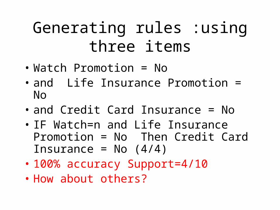
Generating rules :using three items
• Watch Promotion = No• and Life Insurance Promotion = No• and Credit Card Insurance = No • IF Watch=n and Life Insurance Promotion
= No Then Credit Card Insurance = No (4/4)
• 100% accuracy Support=4/10• How about others?
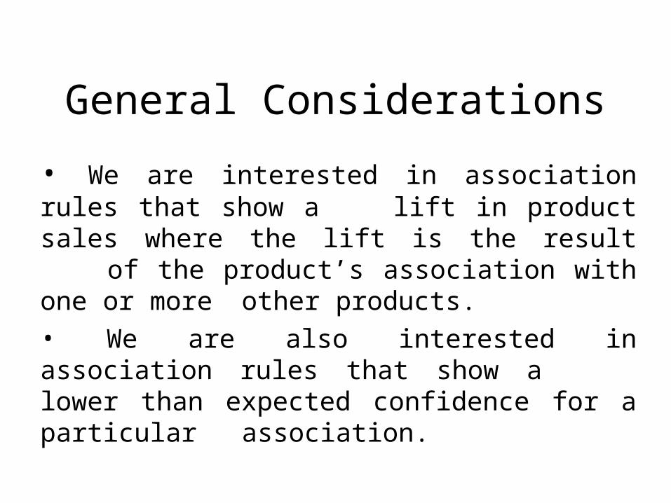
General Considerations
• We are interested in association rules that show a lift in product sales where the lift is the result of the product’s association with one or more other products.
• We are also interested in association rules that show a lower than expected confidence for a particular association.
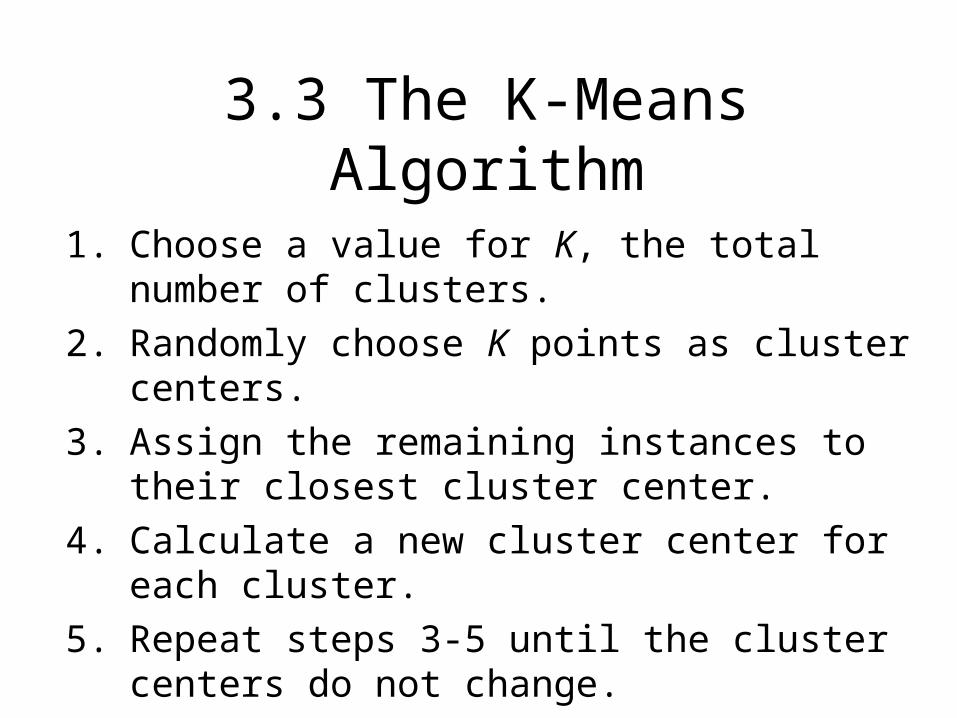
3.3 The K-Means Algorithm
1. Choose a value for K, the total number of clusters.
2. Randomly choose K points as cluster centers.
3. Assign the remaining instances to their closest cluster center.
4. Calculate a new cluster center for each cluster.
5. Repeat steps 3-5 until the cluster centers do not change.
An Example Using K-Means
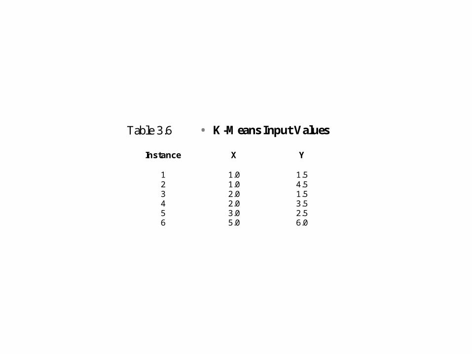
Table 3.6 • K-Means Input Values
Instance X Y
1 1.0 1.52 1.0 4.53 2.0 1.54 2.0 3.55 3.0 2.56 5.0 6.0
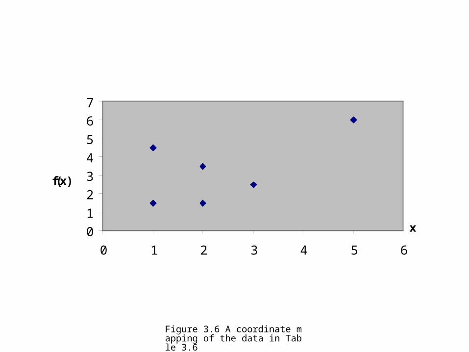
Figure 3.6 A coordinate mapping of the data in Table 3.6
0
1
2
3
4
5
6
7
0 1 2 3 4 5 6
f(x)
x
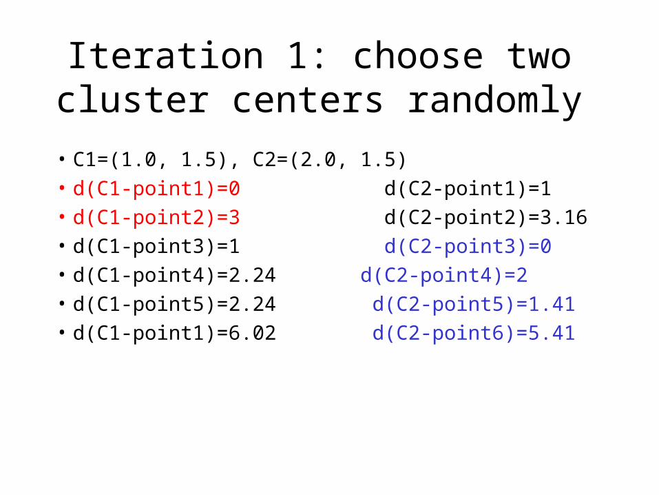
Iteration 1: choose two cluster centers randomly
• C1=(1.0, 1.5), C2=(2.0, 1.5)
• d(C1-point1)=0 d(C2-point1)=1
• d(C1-point2)=3 d(C2-point2)=3.16
• d(C1-point3)=1 d(C2-point3)=0
• d(C1-point4)=2.24 d(C2-point4)=2
• d(C1-point5)=2.24 d(C2-point5)=1.41
• d(C1-point1)=6.02 d(C2-point6)=5.41
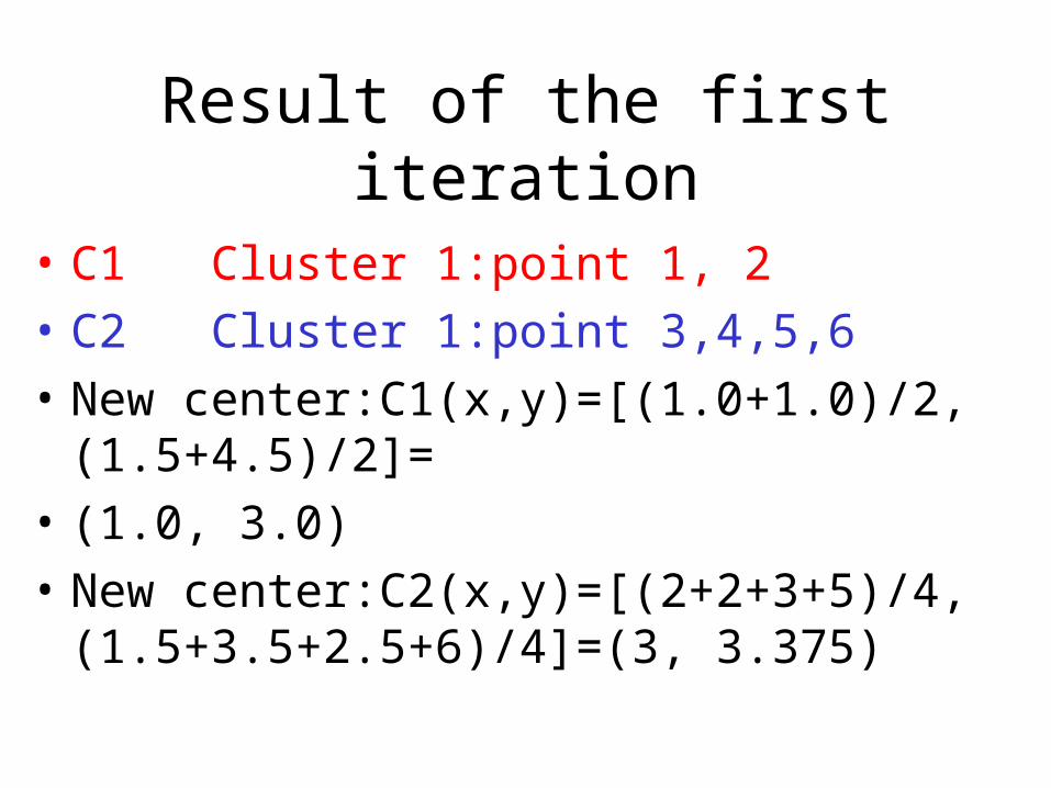
Result of the first iteration
• C1 Cluster 1:point 1, 2
• C2 Cluster 1:point 3,4,5,6
• New center:C1(x,y)=[(1.0+1.0)/2, (1.5+4.5)/2]=
• (1.0, 3.0)
• New center:C2(x,y)=[(2+2+3+5)/4, (1.5+3.5+2.5+6)/4]=(3, 3.375)
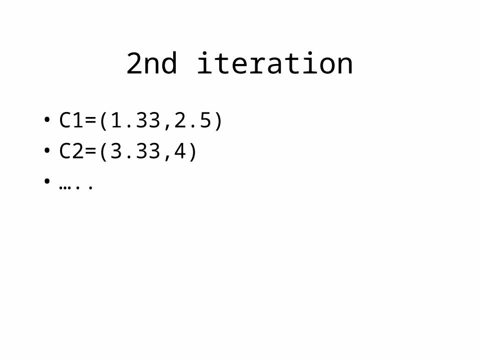
2nd iteration
• C1=(1.33,2.5)
• C2=(3.33,4)
• …..
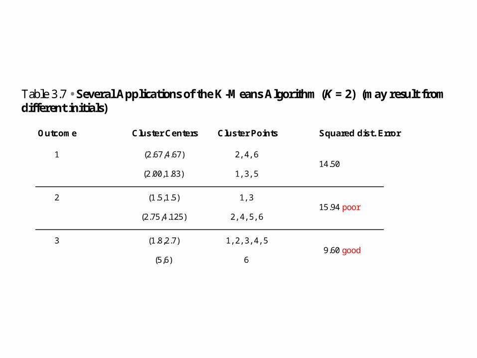
Table 3.7 • Several Applications of the K-Means Algorithm (K = 2) (may result from different initials)
Outcome Cluster Centers Cluster Points Squared dist. Error
1 (2.67,4.67) 2, 4, 6 14.50
(2.00,1.83) 1, 3, 5
2 (1.5,1.5) 1, 3 15.94 poor
(2.75,4.125) 2, 4, 5, 6
3 (1.8,2.7) 1, 2, 3, 4, 5 9.60 good
(5,6) 6
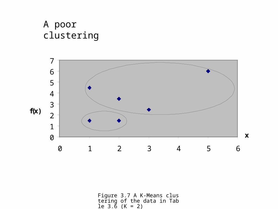
Figure 3.7 A K-Means clustering of the data in Table 3.6 (K = 2)
0
1
2
3
4
5
6
7
0 1 2 3 4 5 6
x
f(x)
A poor clustering
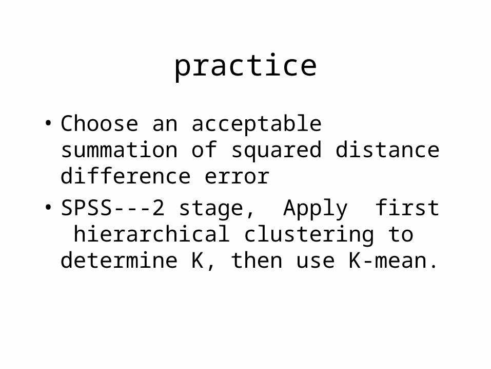
practice
• Choose an acceptable summation of squared distance difference error
• SPSS---2 stage, Apply first hierarchical clustering to determine K, then use K-mean.
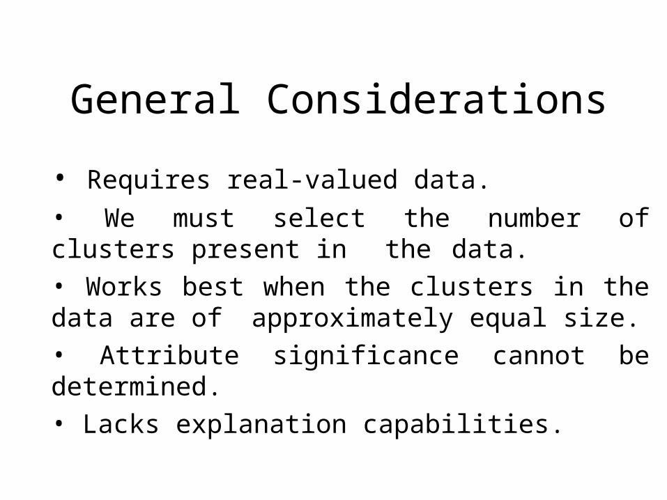
General Considerations
• Requires real-valued data.
• We must select the number of clusters present in the data.
• Works best when the clusters in the data are of approximately equal size.• Attribute significance cannot be determined.• Lacks explanation capabilities.
3.4 Genetic Learning
Genetic Learning Operators
• Crossover
• Mutation
• Selection

Genetic Algorithms and Supervised Learning
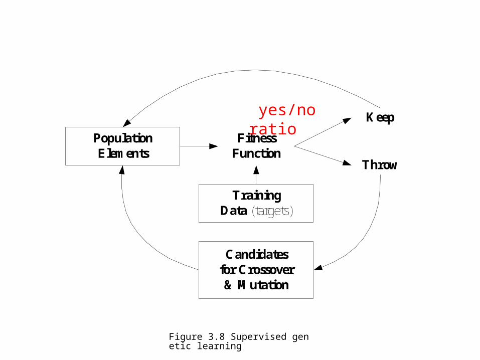
Figure 3.8 Supervised genetic learning
FitnessFunction
PopulationElements
Candidatesfor Crossover& Mutation
TrainingData (targets)
Keep
Throw
yes/no ratio
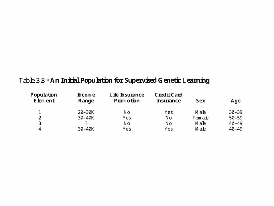
Table 3.8 • An Initial Population for Supervised Genetic Learning
Population Income Life Insurance Credit CardElement Range Promotion Insurance Sex Age
1 20–30K No Yes Male 30–392 30–40K Yes No Female 50–593 ? No No Male 40–494 30–40K Yes Yes Male 40–49
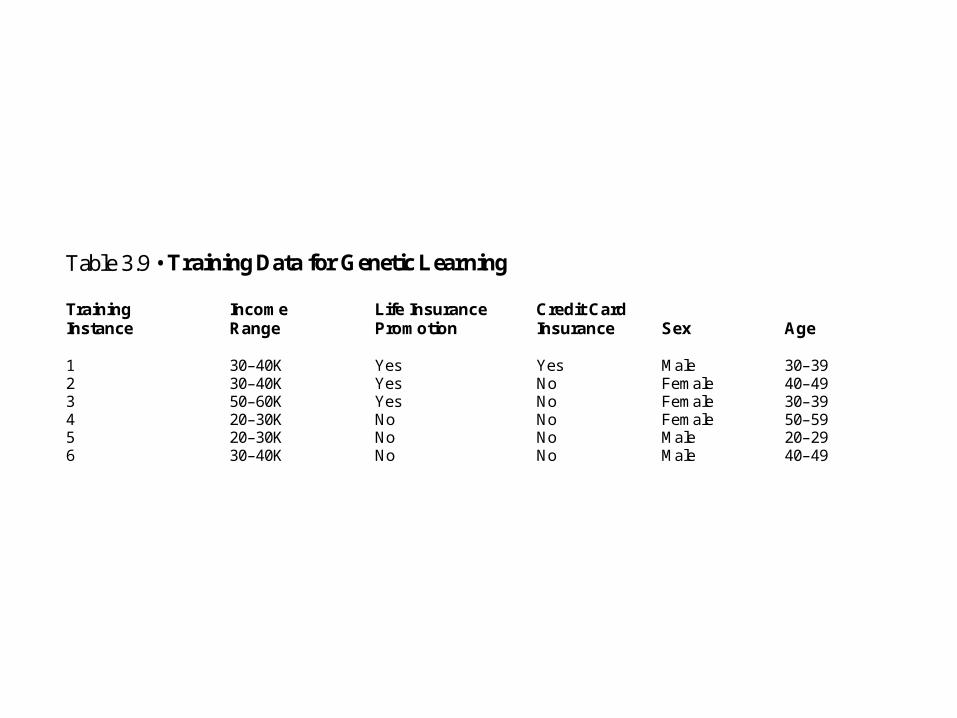
Table 3.9 • Training Data for Genetic Learning
Training Income Life Insurance Credit CardInstance Range Promotion Insurance Sex Age
1 30–40K Yes Yes Male 30–392 30–40K Yes No Female 40–493 50–60K Yes No Female 30–394 20–30K No No Female 50–595 20–30K No No Male 20–296 30–40K No No Male 40–49
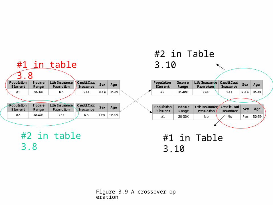
Figure 3.9 A crossover operation
PopulationElement
AgeSexCredit CardInsurance
Life InsurancePromotion
IncomeRange
#1 30-39MaleYesNo20-30K
PopulationElement
AgeSexCredit CardInsurance
Life InsurancePromotion
IncomeRange
#2 50-59FemNoYes30-40K
PopulationElement
AgeSexCredit CardInsurance
Life InsurancePromotion
IncomeRange
#2 30-39MaleYesYes30-40K
PopulationElement
AgeSexCredit CardInsurance
Life InsurancePromotion
IncomeRange
#1 50-59FemNoNo20-30K
#1 in table 3.8
#2 in table 3.8 #1 in Table 3.10
#2 in Table 3.10
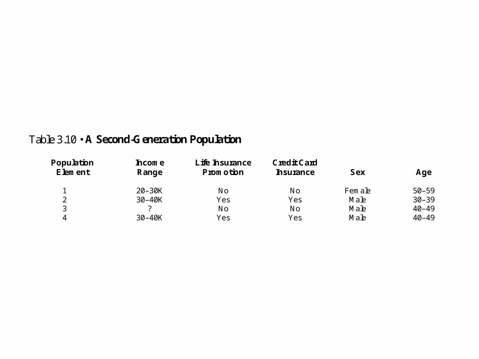
Table 3.10 • A Second-Generation Population
Population Income Life Insurance Credit CardElement Range Promotion Insurance Sex Age
1 20–30K No No Female 50–592 30–40K Yes Yes Male 30–393 ? No No Male 40–494 30–40K Yes Yes Male 40–49
• Test: – New instance will be compared with all
instances and be assigned the same class as the most similar instance compared.
• Or randomly choose any one in the final population and assigned the same class …
Genetic Algorithms and Unsupervised Clustering
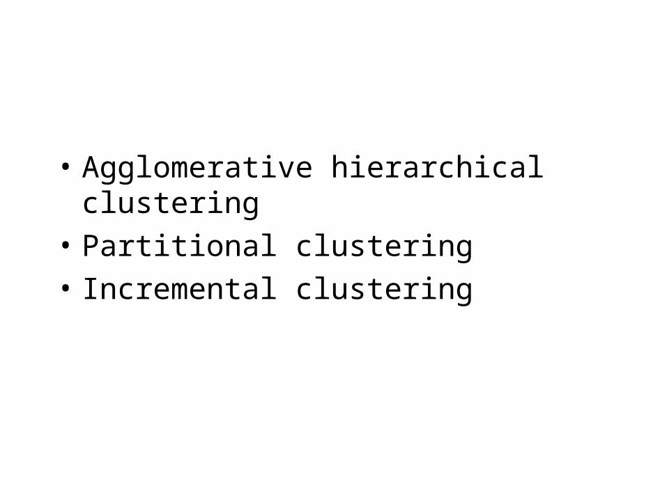
• Agglomerative hierarchical clustering
• Partitional clustering
• Incremental clustering
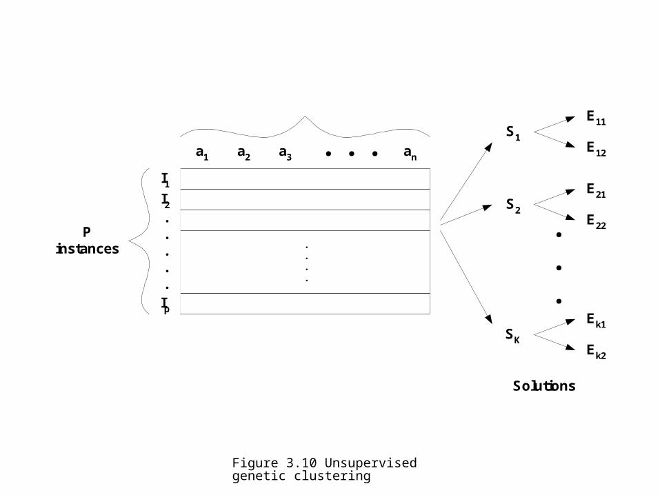
Figure 3.10 Unsupervised genetic clustering
a1 a2 a3 . . . an
.
.
.
.
I1
Ip
I2.....
Pinstances
S1
Ek2
Ek1
E22
E21
E12
E11
SK
S2
Solutions
.
.
.
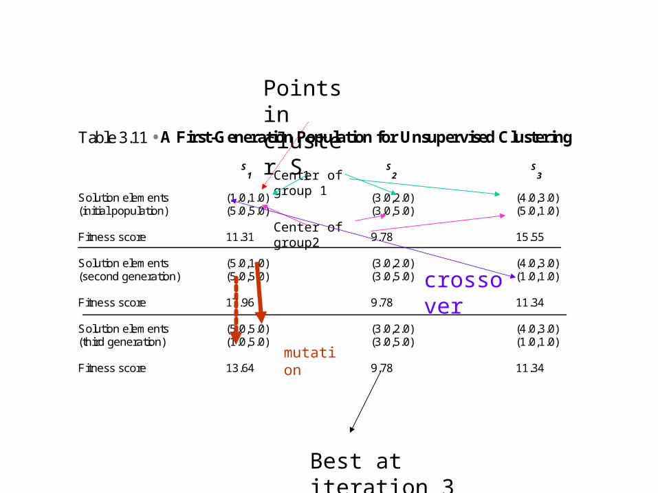
Table 3.11 • A First-Generation Population for Unsupervised Clustering
S1
S2
S3
Solution elements (1.0,1.0) (3.0,2.0) (4.0,3.0)(initial population) (5.0,5.0) (3.0,5.0) (5.0,1.0)
Fitness score 11.31 9.78 15.55
Solution elements (5.0,1.0) (3.0,2.0) (4.0,3.0)(second generation) (5.0,5.0) (3.0,5.0) (1.0,1.0)
Fitness score 17.96 9.78 11.34
Solution elements (5.0,5.0) (3.0,2.0) (4.0,3.0)(third generation) (1.0,5.0) (3.0,5.0) (1.0,1.0)
Fitness score 13.64 9.78 11.34
Points in cluster S1
Center of group 1
Center of group2
crossover
mutation
Best at iteration 3
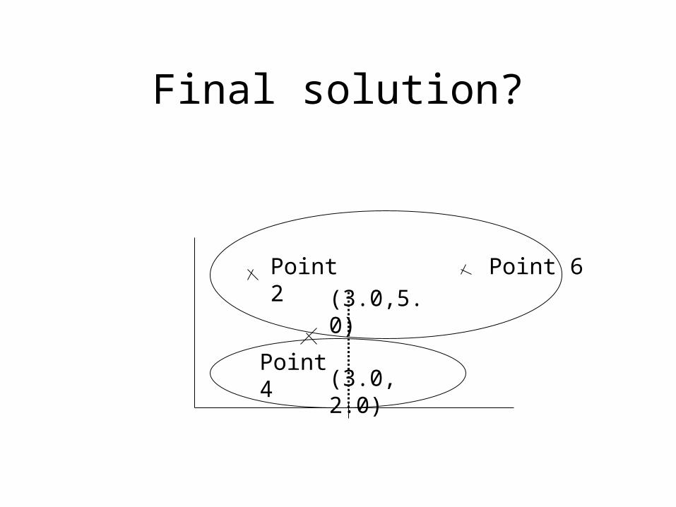
Final solution?
(3.0, 2.0)
(3.0,5.0)
Point 2 Point 6
Point 4

homework
• Demonstrate Table 3.11
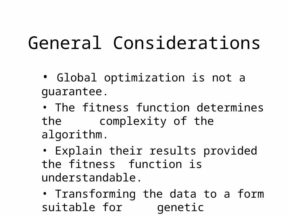
General Considerations
• Global optimization is not a guarantee.
• The fitness function determines the complexity of the algorithm.• Explain their results provided the fitness function is understandable.• Transforming the data to a form suitable for
genetic learning can be a challenge.
3.5 Choosing a Data Mining Technique
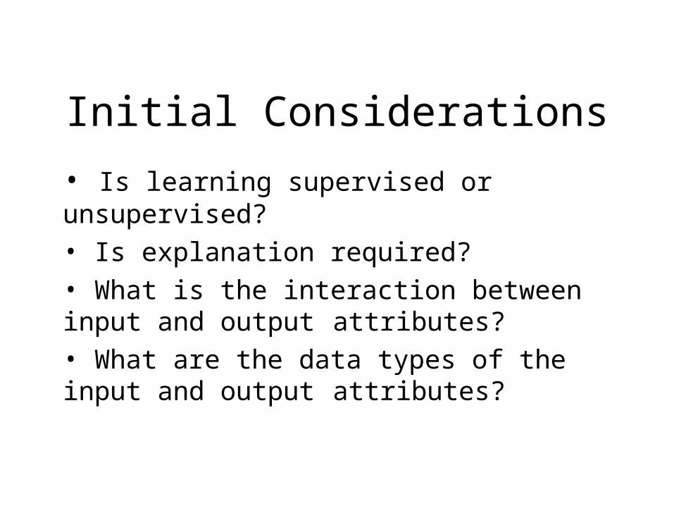
Initial Considerations
• Is learning supervised or unsupervised?
• Is explanation required?• What is the interaction between input and output attributes?• What are the data types of the input and output attributes?
Further Considerations
• Do We Know the Distribution of the Data?
• Do We Know Which Attributes Best Define the Data?• Does the Data Contain Missing Values?• Is Time an Issue?• Which Technique Is Most Likely to Give a Best Test
Set Accuracy?