BASIC DETONATION PHYSICS ALGORITHMSBasic Detonation Physics Algorithms N/A N/A 62602F 2502 67 63 Douglas V. Nance AFRL/RWPC 101 W. Eglin Blvd. Eglin AFB, FL 32542-6810 AFRL-RW-EG-TR-2011-159

AFRL-RW-EG-TR-2011-159

BASIC DETONATION PHYSICS ALGORITHMS

Douglas V. Nance

AFRL/RWPC

101 W. Eglin Blvd. Eglin AFB, FL 32542-6810

December 2011

INTERIM REPORT

AIR FORCE RESEARCH LABORATORY MUNITIONS DIRECTORATE

Air Force Materiel Command Force MaterialCommand

United States Air Force Eglin Air Force Base, FL 32542

DISTRIBUTION A. Approved for public release, distribution unlimited. 96th ABW/PA

Approval and Clearance # 96ABW-2011-0548 dated 28 November 2011.

NOTICE AND SIGNATURE PAGE

Using Government drawings, specifications, or other data included in this document for any purpose other than Government procurement does not in any obligate the U.S. Government. The fact that the Government formulated or supplied the drawings, specifications, or other data does not license the holder or any other person or corporation, or convey any rights or permission to manufacture, use, or sell any patented invention that may relate to them. This report was cleared for public release by the 96th Air Base Wing, Public Affairs Office, and is available to the general public, including foreign nationals. Copies may be obtained from the Defense Technical Information Center (DTIC) < http://www.dtic.mil/dtic/index/html>.

AFRL-RW-EG-TR-2011- HAS BEEN REVIEWED AND IS APPROVED FOR PUBLICATION IN ACCORDANCE WITH ASSIGNED DISTRIBUTION STATEMENT. FOR THE DIRECTOR: ______________________________________ _____________________________________ Craig M. Ewing, DR-IV, PhD Douglas V. Nance Technical Adviser Program Manager Strategic Planning and Assessment Division

This report is published in the interest of scientific and technical information exchange, and its publication does not constitute the Government’s approval or disapproval of its ideas or findings.

159

ORIGINAL SIGNED ORIGINAL SIGNED

Standard Form 298 (Rev. 8/98)

REPORT DOCUMENTATION PAGE

Prescribed by ANSI Std. Z39.18

Form Approved OMB No. 0704-0188

The public reporting burden for this collection of information is estimated to average 1 hour per response, including the time for reviewing instructions, searching existing data sources, gathering and maintaining the data needed, and completing and reviewing the collection of information. Send comments regarding this burden estimate or any other aspect of this collection of information, including suggestions for reducing the burden, to Department of Defense, Washington Headquarters Services, Directorate for Information Operations and Reports (0704-0188), 1215 Jefferson Davis Highway, Suite 1204, Arlington, VA 22202-4302. Respondents should be aware that notwithstanding any other provision of law, no person shall be subject to any penalty for failing to comply with a collection of information if it does not display a currently valid OMB control number. PLEASE DO NOT RETURN YOUR FORM TO THE ABOVE ADDRESS. 1. REPORT DATE (DD-MM-YYYY) 2. REPORT TYPE 3. DATES COVERED (From - To)

4. TITLE AND SUBTITLE 5a. CONTRACT NUMBER

5b. GRANT NUMBER

5c. PROGRAM ELEMENT NUMBER

5d. PROJECT NUMBER

5e. TASK NUMBER

5f. WORK UNIT NUMBER

6. AUTHOR(S)

7. PERFORMING ORGANIZATION NAME(S) AND ADDRESS(ES) 8. PERFORMING ORGANIZATION REPORT NUMBER

9. SPONSORING/MONITORING AGENCY NAME(S) AND ADDRESS(ES) 10. SPONSOR/MONITOR'S ACRONYM(S)

11. SPONSOR/MONITOR'S REPORT NUMBER(S)

12. DISTRIBUTION/AVAILABILITY STATEMENT

13. SUPPLEMENTARY NOTES

14. ABSTRACT

15. SUBJECT TERMS

16. SECURITY CLASSIFICATION OF: a. REPORT b. ABSTRACT c. THIS PAGE

17. LIMITATION OF ABSTRACT

18. NUMBER OF PAGES

19a. NAME OF RESPONSIBLE PERSON

19b. TELEPHONE NUMBER (Include area code)

01-12-2011 INTERIM 01-10-2011 - 31-10-2011

Basic Detonation Physics Algorithms N/A

N/A

62602F

2502

67

63

Douglas V. Nance

AFRL/RWPC 101 W. Eglin Blvd. Eglin AFB, FL 32542-6810


AFRL/RWPC 101 W. Eglin Blvd. Eglin AFB, FL 32542-6810

AFRL-RW-EG


Distribution A: Approved for public release, distribution unlimited. (96ABW-2011-0548) 28 Nov 11

NONE

This report presents the theory behind a series of detonation physics algorithms used to simulate the detonation of a condensed explosive. The numerical scheme implemented in this case is the Roe flux difference splitting scheme due to Glaister. This report contains a detailed discussion of the mathematical derivation along with a printing of the source code. We also include a discussion of methods for implementing Lagrangian tracking algorithms for solid inclusions within the condensed explosive.

detonation, explosive, flux, jacobian

UNCLAS UNCLAS UNCLAS UL 102

Douglas V. Nance

Reset

Distribution A. Approved for public release, distribution unlimited. (96ABW-2011-0548) i

TABLE OF CONTENTS

Section Page 1 INTRODUCTION 1 1.0 Numerical Detonation Physics 1 1.1 A Map for this Report 2 2 GOVERNING EQUATIONS 4 2.1 The Reactive Euler Equations 4 2.2 Mixture Equations of State 5 2.3 Solid Explosive Equations of State 6 2.4 Detonation Products Equation of State 8 3 SYSTEM EIGEN-STRUCTURE 10 3.1 Flux Jacobian Matrices 10 3.2 Eigenvalues 12 3.3 Eigenvectors 13 4 BUILDING THE NUMERICAL SCHEME 18 4.1 Pressure Derivatives 18 4.2 Finite Volume Discretization 21 4.3 Temporal Discretization 22 4.4 The Numerical Flux 23 4.5 A Higher Order Scheme 25 4.6 Boundary Conditions 27 5 PARTICLE MOTION 28 5.1 Coupling Terms 28 5.2 Particle Laws of Motion 29 6 RESULTS 32 6.1 Simple Plane Wave Detonation 32 6.2 Detonation of Pure HMX 35 6.3 Detonation of HMX Containing Metal Particles 37

Distribution A. Approved for public release, distribution unlimited. (96ABW-2011-0548) ii

7 CONCLUSIONS 39 8 RECOMMENDATIONS 39 REFERENCES 40 APP. A SOURCE CODE 42

Distribution A. Approved for public release, distribution unlimited. (96ABW-2011-0548) iii

LIST OF FIGURES

Figure Page 1 Interface Notation 23 2 Problem 1 Detonation Field Density, Time 3.0 33 3 Problem 1 Detonation Field Velocity, Time 3.0 33 4 Problem 1 Detonation Field Pressure, Time 3.0 34 5 Problem 1 Detonation Field Reaction Progress Variable, Time 3.0 34 6 Numerical Detonation Solution Hayes-I/JWL in HMX at 3 μs. Horizontal Axis is Distance in Meters 36 7 Numerical Detonation Solution Hayes-II/JWL in HMX at 3 μs. Horizontal Axis is Distance in Meters 36 8 Radial Locations for Steel Particles Embedded in a Mass of Detonating HMX 37 9 Radial Velocities for Steel Particles Embedded in a Detonating Mass of HMX 38

Distribution A. Approved for public release, distribution unlimited. (96ABW-2011-0548)

1 INTRODUCTION Steady increases in large scale circuit integration indicate that the Twenty-First Century will promise significant advances in High Performance Computing (HPC) machinery. Today, one may obtain desk-side Linux systems containing eight processors (and thirty-two or more cores) for comparatively reasonable prices. Moreover, common laptop systems wield significant computing power with central processing unit (CPU) speeds in the neighborhood of 3.0 GHz (maybe more by the time this report is certified) and random access memory (RAM) storage capability in hundreds of Gigabytes (GB). In the realm of “Big Iron”, the Department of Defense (DoD) High Performance Computing (HPC) Modernization Office recently began operating clusters each with tens of thousands of cores, and the Department of Energy laboratory community has even larger systems. These developments have significant implications for the relatively small Computational Physics research community. This research community represented by disciplines such as high energy physics, quantum chemistry and computational fluid dynamics has an ever increasing need for computer memory and for parallel processing speed. Computational Fluid Dynamics (CFD) has drawn on HPC resources for many years to help with aircraft and fluid system design. Some problems like high Reynolds number direct numerical simulations are still computationally inaccessible, but these situations are fewer in number than just one decade ago. For instance, we routinely solve problems involving the large eddy simulation (LES) of compressible turbulence with good results. Older techniques such as Reynolds-Averaged Navier-Stokes (RANS) simulation now teeter on the brink of obsolescence. Moreover, massive computing power now permits us to invade new territory previously relegated to analytical solutions supported by many assumptions and highly simplified, under-resolved computational studies. Quantum physics now benefits widely from HPC science in the areas of quantum chemistry and molecular dynamics. These areas of physics now impact design engineering. Although it occupies only a very small part of the research community, detonation physics, a close relative of CFD, can benefit handsomely from ever more powerful computational techniques and equipment. 1.0 Numerical Detonation Physics Numerical Detonation Physics applies many of the same computational techniques employed by CFD. The primary reason is because detonations are powered by the propagation of the detonation wave, a powerful shock wave that transforms the unreacted explosive into detonation product species. Like the shock waves encountered in transonic and supersonic flow, detonation waves must be “captured” in the material field by using special numerical techniques. Gas phase detonations, e.g., the explosive burn of acetylene gas, are true detonations but they lack some of the complexity associated with the detonation of condensed (solid or liquid) explosives. Gas phase detonation is usually initiated by high temperature. It follows that temperature is the dominant term in the reaction rate expression. One should also not make light of the fact that we actually have


2

good, quantitative models for gas phase detonation chemistry. The science behind the detonation of condensed explosives is not so evolved. The detonation of a condensed explosive is most often modeled as a shock-driven process. Macroscopic observation seems to indicate that a shock wave is often required to detonate these explosives. Many solid explosives simply “burn” when exposed to a flame, at least when considered over relatively short time periods. Exposure to a shock impulse is often needed to initiate the run to detonation for an explosive. This physics problem is complicated greatly because of the smallness of scales concerning the detonation wave. The detonation wave covers a thin region, a fraction of a millimeter for most ideal or Carbon-Hydrogen-Nitrogen-Oxygen (CHNO) explosives like Trinitro-toluene (TNT). The head of the detonation wave lies at the entrance to the detonation reaction zone. This is the tiny region in space where the detonation chemical reactions take place. For condensed explosives, we do not know these chemical reactions. We know only, in some sense, their end products, and if we detonate two like samples of an explosive, we may obtain two different product spectrums. For this reason, condensed explosives are relatively crude chemical mixtures. Still, the detonation process itself may be addressed by the direct application of the conservation laws for mass, momentum and energy. This same approach is used for CFD problems, but for explosives we are required to apply equations of state for both the unreacted explosive material and the detonation products. It is also important that we consider heterogeneous explosives. These materials contain non-explosive additives like plastic binders and metal particles. In future treatments of this problem, we will also be required to treat the material behavior (material strength versus applied stress) of the solid explosive in response to shock excitation. 1.1 A Map for this Report This report is intended to assist in the process of transitioning detonation physics algorithms into the Large Eddy Simulation with LInear Eddy Modeling in 3 Dimensions (LESLIE3D) multiphase physics computer program. The discussions that follow describe the algorithms applied in the source code included in Appendix A. Although these algorithms are tested and validated to some extent, it is nont recommended that they be coded directly into LESLIE3D. Rather, the Harten, Lax and van Leer (HLL) family of algorithms should be used for flux difference splitting in lieu of Roe’s method. Moreover, inhomogeneous terms in the equations should be addressed through Strang splitting.1

The report is organized as follows. In Section 2, we describe the governing equations for the detonation problem based upon the work of Xu et al.2 Within this set of equations, we add the terms coupling the detonation flow field to the particle field. We show that reaction rate, particle coupling and geometric effects may be incorporated as source terms. The equations of state used for the solid explosive and for the detonation products are also presented in this section. The advective terms, of critical importance in the shock-capturing scheme, are clearly delineated. Section 3 describes the eigen-structure for the system of governing equations. The flux Jacobian matrix is developed


3

for the reactive Euler equations adapted for a real gas equation of state. Then we develop a set of eigenvalues and eigenvectors needed in order to accurately capture the detonation wave. In Section 4, we discuss the overall numerical scheme and temporal discretization procedure used in our detonation computer program. We also discuss the development of the numerical flux vector in detail. Section 5 contains the terms governing the motion of Lagrangian particles including the drag laws. In Section 6, we provide the results for three example calculations. After performing a calculation to verify proper code performance, we simulate the detonation of a spherical mass of HMX loaded with metal particles. We show a series of detonation waveforms for this explosive, and we go on to include the resulting particle trajectories and velocities. We also make some basic comparisons between the results produced by our computer program to archival explosive performance data for HMX. Finally, in Section 7, we draw several important conclusions from our development. We also make recommendations for follow-on work needed to support the installation of detonation physics algorithms in LESLIE3D.


4

2 GOVERNING EQUATIONS

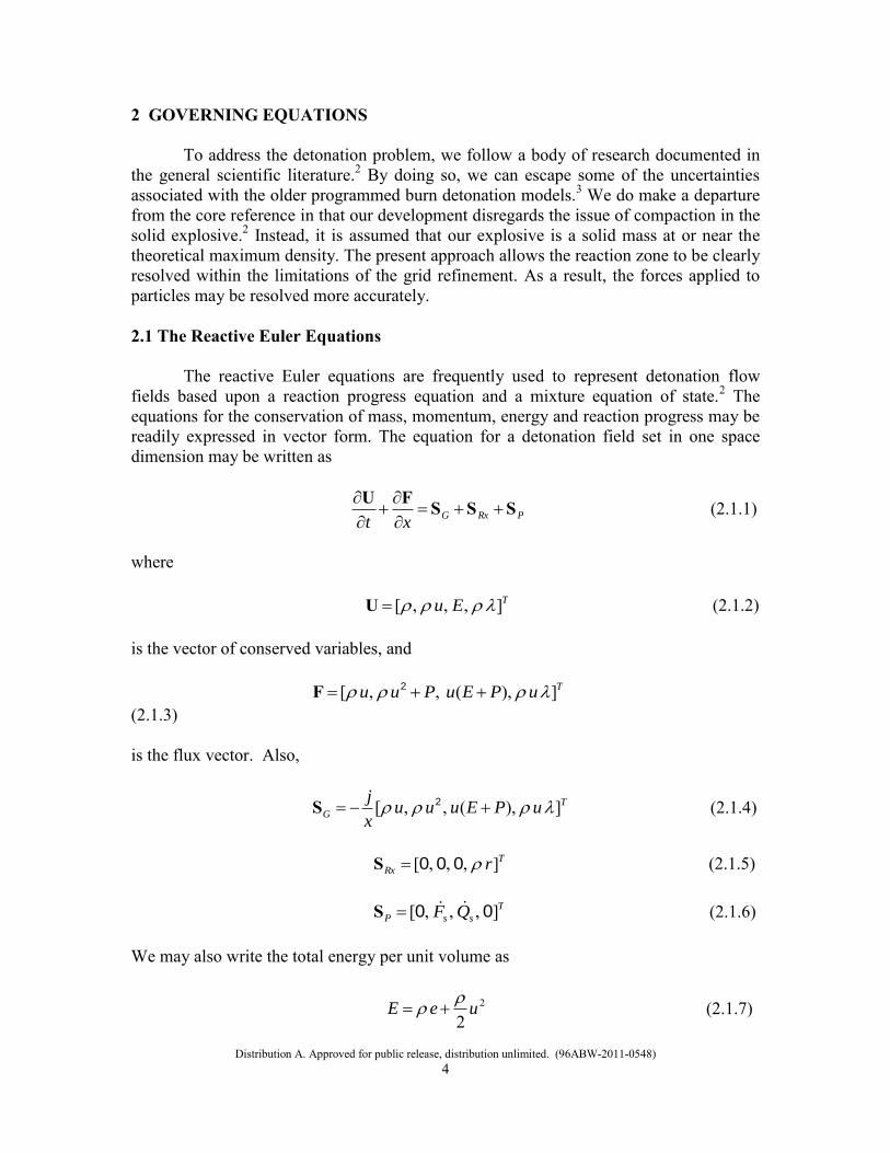
To address the detonation problem, we follow a body of research documented in the general scientific literature.2 By doing so, we can escape some of the uncertainties associated with the older programmed burn detonation models.3 We do make a departure from the core reference in that our development disregards the issue of compaction in the solid explosive.2 Instead, it is assumed that our explosive is a solid mass at or near the theoretical maximum density. The present approach allows the reaction zone to be clearly resolved within the limitations of the grid refinement. As a result, the forces applied to particles may be resolved more accurately. 2.1 The Reactive Euler Equations The reactive Euler equations are frequently used to represent detonation flow fields based upon a reaction progress equation and a mixture equation of state.2 The equations for the conservation of mass, momentum, energy and reaction progress may be readily expressed in vector form. The equation for a detonation field set in one space dimension may be written as

PRxGxt

SSSFU

(2.1.1)

where TEu ],,,[ U (2.1.2) is the vector of conserved variables, and TuPEuPuu ]),(,,[ 2F (2.1.3) is the flux vector. Also,

T

G uPEuuux

j ]),(,,[ 2S (2.1.4)

T

Rx r],,,[ 000S (2.1.5) T

ssP QF ],,,[ 00 S (2.1.6) We may also write the total energy per unit volume as

2

2ueE

(2.1.7)


5

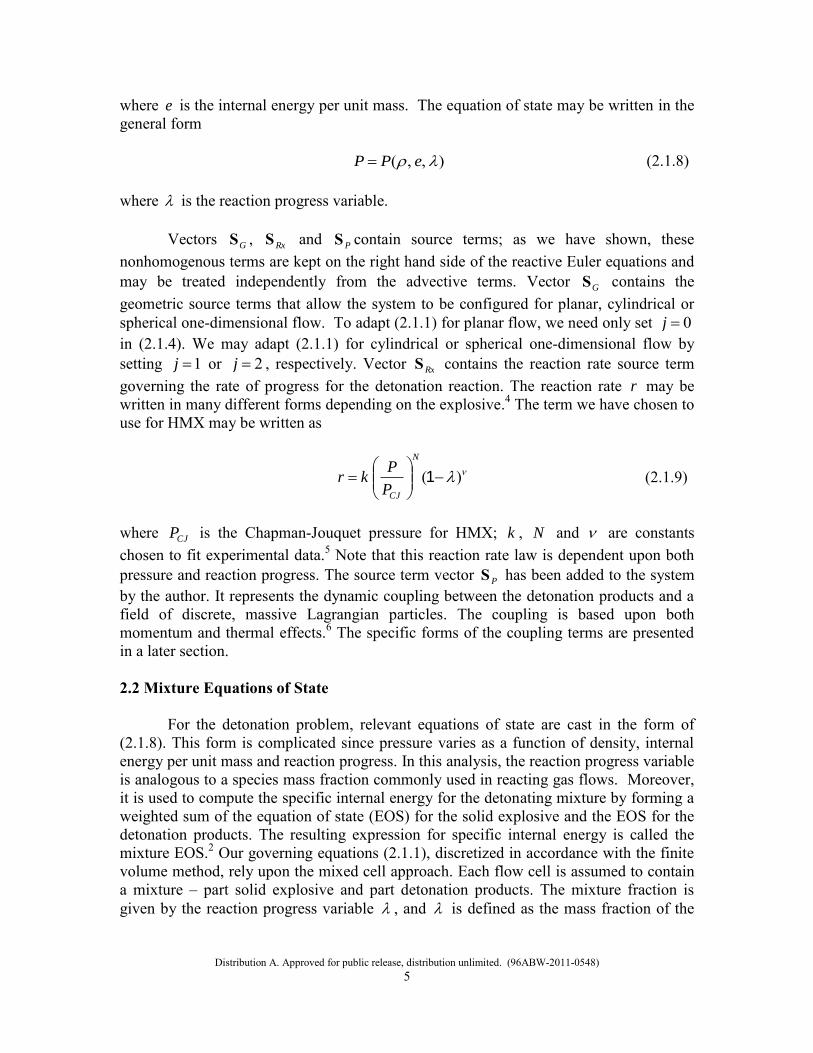
where e is the internal energy per unit mass. The equation of state may be written in the general form ),,( ePP (2.1.8) where is the reaction progress variable. Vectors GS , RxS and PS contain source terms; as we have shown, these nonhomogenous terms are kept on the right hand side of the reactive Euler equations and may be treated independently from the advective terms. Vector GS contains the geometric source terms that allow the system to be configured for planar, cylindrical or spherical one-dimensional flow. To adapt (2.1.1) for planar flow, we need only set 0j

in (2.1.4). We may adapt (2.1.1) for cylindrical or spherical one-dimensional flow by setting 1j or 2j , respectively. Vector RxS contains the reaction rate source term governing the rate of progress for the detonation reaction. The reaction rate r may be written in many different forms depending on the explosive.4 The term we have chosen to use for HMX may be written as

)(

1

N

CJP

Pkr (2.1.9)

where CJP is the Chapman-Jouquet pressure for HMX; k , N and are constants chosen to fit experimental data.5 Note that this reaction rate law is dependent upon both pressure and reaction progress. The source term vector PS has been added to the system by the author. It represents the dynamic coupling between the detonation products and a field of discrete, massive Lagrangian particles. The coupling is based upon both momentum and thermal effects.6 The specific forms of the coupling terms are presented in a later section. 2.2 Mixture Equations of State For the detonation problem, relevant equations of state are cast in the form of (2.1.8). This form is complicated since pressure varies as a function of density, internal energy per unit mass and reaction progress. In this analysis, the reaction progress variable is analogous to a species mass fraction commonly used in reacting gas flows. Moreover, it is used to compute the specific internal energy for the detonating mixture by forming a weighted sum of the equation of state (EOS) for the solid explosive and the EOS for the detonation products. The resulting expression for specific internal energy is called the mixture EOS.2 Our governing equations (2.1.1), discretized in accordance with the finite volume method, rely upon the mixed cell approach. Each flow cell is assumed to contain a mixture – part solid explosive and part detonation products. The mixture fraction is given by the reaction progress variable , and is defined as the mass fraction of the


6

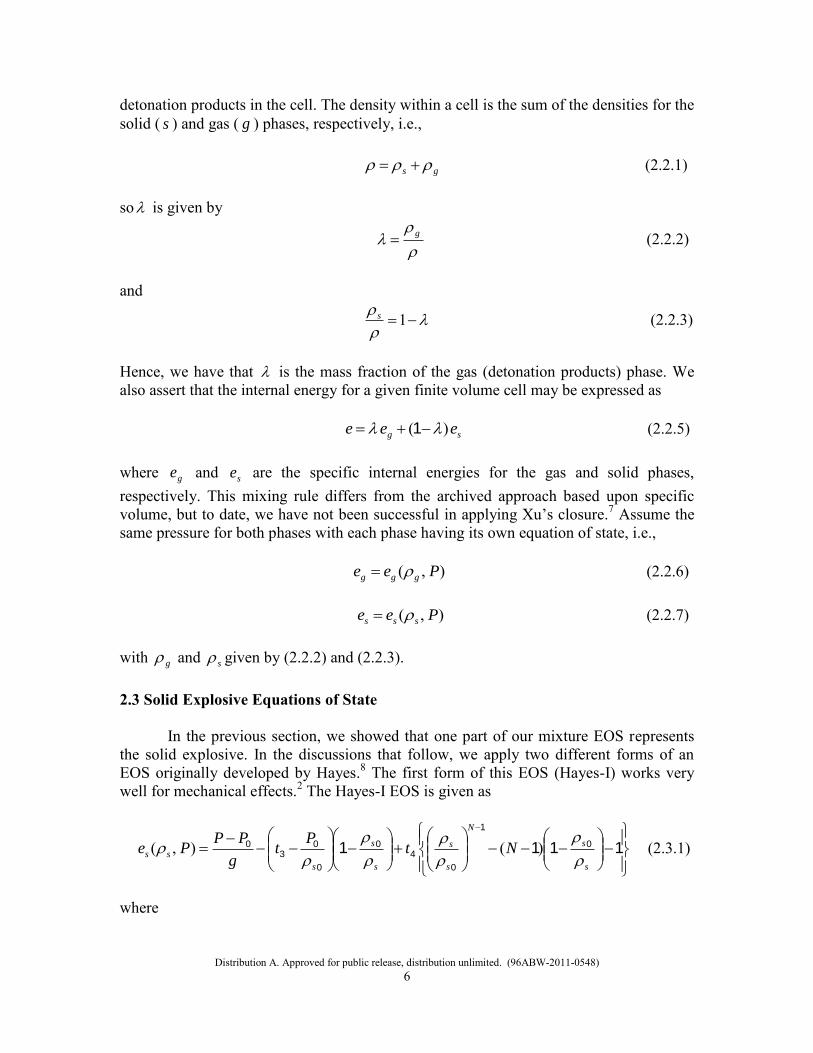
detonation products in the cell. The density within a cell is the sum of the densities for the solid ( s ) and gas ( g ) phases, respectively, i.e., gs (2.2.1) so is given by

g (2.2.2)

and

1s (2.2.3)

Hence, we have that is the mass fraction of the gas (detonation products) phase. We also assert that the internal energy for a given finite volume cell may be expressed as sg eee )( 1 (2.2.5) where ge and se are the specific internal energies for the gas and solid phases, respectively. This mixing rule differs from the archived approach based upon specific volume, but to date, we have not been successful in applying Xu’s closure.7 Assume the same pressure for both phases with each phase having its own equation of state, i.e., ),( Pee ggg (2.2.6) ),( Pee sss (2.2.7) with g and s given by (2.2.2) and (2.2.3). 2.3 Solid Explosive Equations of State In the previous section, we showed that one part of our mixture EOS represents the solid explosive. In the discussions that follow, we apply two different forms of an EOS originally developed by Hayes.8 The first form of this EOS (Hayes-I) works very well for mechanical effects.2 The Hayes-I EOS is given as

1111 0

1

0

40

0

03

0

s

s

N

s

s

s

s

s

ss NtP

tg

PPPe

)(),( (2.3.1)

where


7

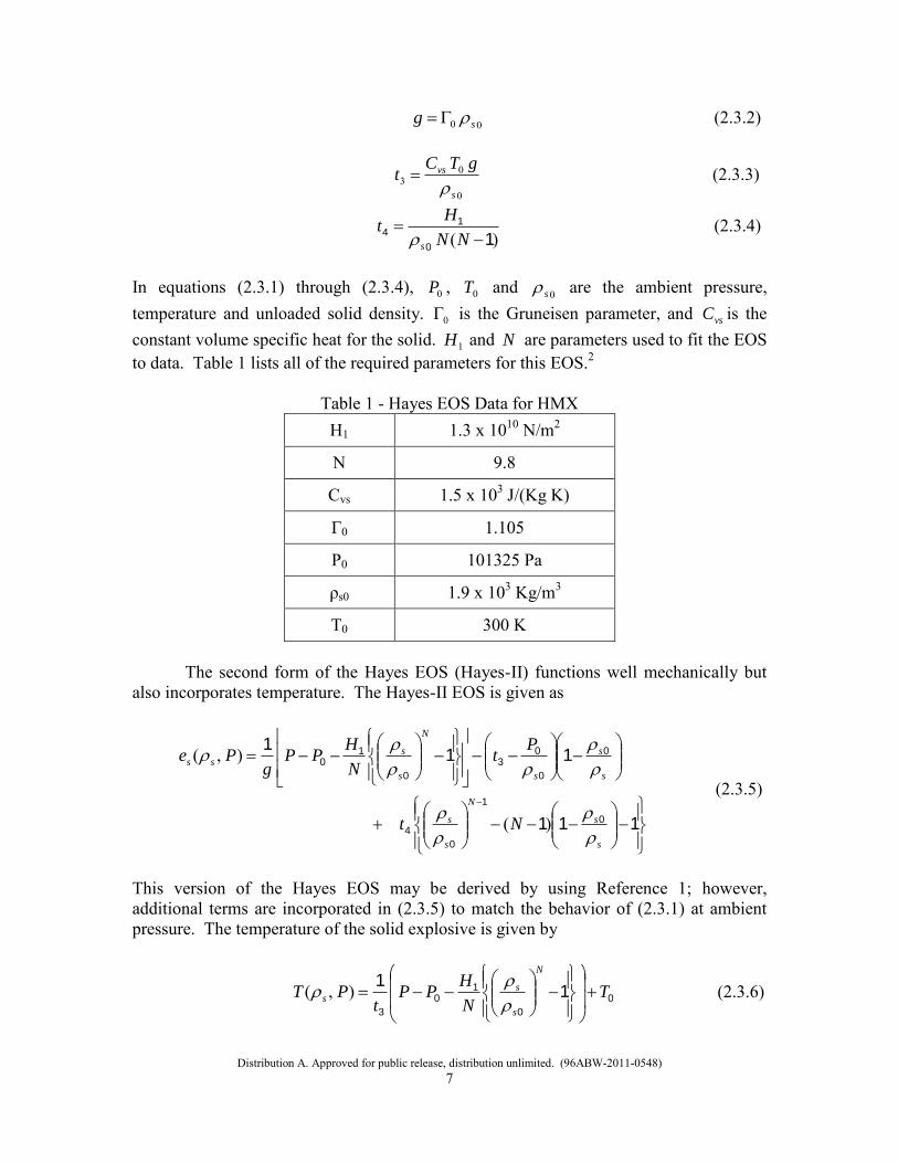
00 sg (2.3.2)

0

03

s

vs gTCt

(2.3.3)

)( 1

0

14

NN

Ht

s (2.3.4)

In equations (2.3.1) through (2.3.4), 0P , 0T and 0s are the ambient pressure, temperature and unloaded solid density. 0 is the Gruneisen parameter, and vsC is the constant volume specific heat for the solid. 1H and N are parameters used to fit the EOS to data. Table 1 lists all of the required parameters for this EOS.2

Table 1 - Hayes EOS Data for HMX

H1 1.3 x 1010 N/m2

N 9.8

Cvs 1.5 x 103 J/(Kg K)

Γ0 1.105

P0 101325 Pa

ρs0 1.9 x 103 Kg/m3

T0 300 K The second form of the Hayes EOS (Hayes-II) functions well mechanically but also incorporates temperature. The Hayes-II EOS is given as

111

111

0

1

0

4

0

0

03

0

10

s

s

N

s

s

s

s

s

N

s

sss

Nt

Pt

N

HPP

gPe

)(

),(

(2.3.5)

This version of the Hayes EOS may be derived by using Reference 1; however, additional terms are incorporated in (2.3.5) to match the behavior of (2.3.1) at ambient pressure. The temperature of the solid explosive is given by

0

0

10

3

11

TN

HPP

tPT

N

s

ss

),( (2.3.6)


8

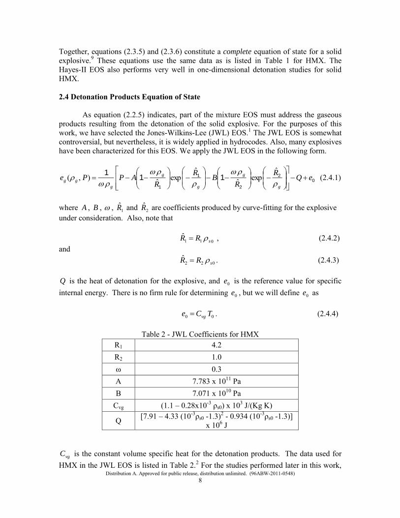
Together, equations (2.3.5) and (2.3.6) constitute a complete equation of state for a solid explosive.9 These equations use the same data as is listed in Table 1 for HMX. The Hayes-II EOS also performs very well in one-dimensional detonation studies for solid HMX. 2.4 Detonation Products Equation of State As equation (2.2.5) indicates, part of the mixture EOS must address the gaseous products resulting from the detonation of the solid explosive. For the purposes of this work, we have selected the Jones-Wilkins-Lee (JWL) EOS.1 The JWL EOS is somewhat controversial, but nevertheless, it is widely applied in hydrocodes. Also, many explosives have been characterized for this EOS. We apply the JWL EOS in the following form.

02

2

1

1

111

eQR

RB

R

RAPPe

g

g

g

g

g

gg

êxpˆ

êxpˆ),( (2.4.1)

where A , B , , 1R and 2R are coefficients produced by curve-fitting for the explosive under consideration. Also, note that 011

ˆsRR , (2.4.2)

and 022

ˆsRR . (2.4.3)

Q is the heat of detonation for the explosive, and 0e is the reference value for specific internal energy. There is no firm rule for determining 0e , but we will define 0e as 00 TCe vg . (2.4.4)

Table 2 - JWL Coefficients for HMX R1 4.2 R2 1.0 ω 0.3 A 7.783 x 1011 Pa B 7.071 x 1010 Pa

Cvg (1.1 – 0.28x10-3 ρs0) x 103 J/(Kg K)

Q [7.91 – 4.33 (10-3ρs0 -1.3)2 - 0.934 (10-3ρs0 -1.3)] x 106 J

vgC is the constant volume specific heat for the detonation products. The data used for HMX in the JWL EOS is listed in Table 2.2 For the studies performed later in this work,


9

we select one of the Hayes equations of state in combination with the JWL EOS to form a mixture EOS.


10

3 SYSTEM EIGEN-STRUCTURE

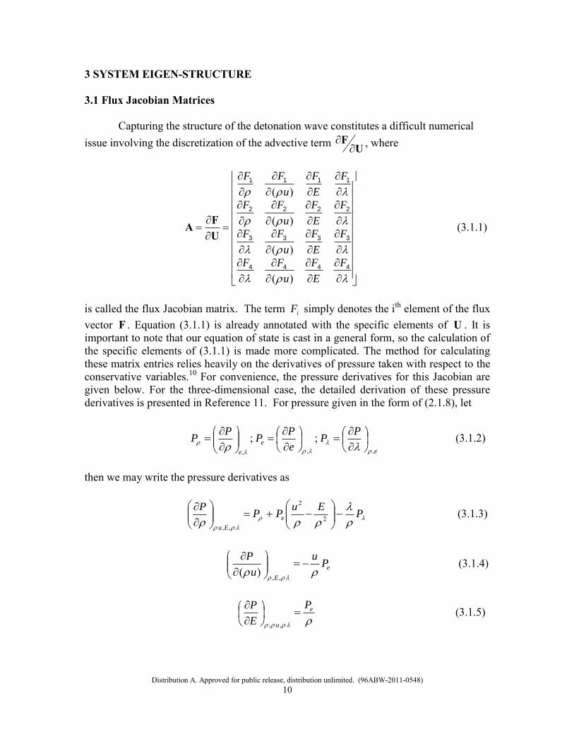
3.1 Flux Jacobian Matrices Capturing the structure of the detonation wave constitutes a difficult numerical issue involving the discretization of the advective term U

F

, where

4444

3333

2222

1111

F

E

F

u

FF

F

E

F

u

FF

F

E

F

u

FF

F

E

F

u

FF

)(

)(

)(

)(

UFA (3.1.1)

is called the flux Jacobian matrix. The term iF simply denotes the ith element of the flux vector F . Equation (3.1.1) is already annotated with the specific elements of U . It is important to note that our equation of state is cast in a general form, so the calculation of the specific elements of (3.1.1) is made more complicated. The method for calculating these matrix entries relies heavily on the derivatives of pressure taken with respect to the conservative variables.10 For convenience, the pressure derivatives for this Jacobian are given below. For the three-dimensional case, the detailed derivation of these pressure derivatives is presented in Reference 11. For pressure given in the form of (2.1.8), let

e

e

e

PP

e

PP

PP

,,,

;;

(3.1.2)

then we may write the pressure derivatives as

P

EuPP

Pe

Eu

2

2

,,

(3.1.3)

e

E

Pu

u

P

,,)( (3.1.4)

e

u

P

E

P

,,

(3.1.5)


11

PP

u

,,)( (3.1.6)

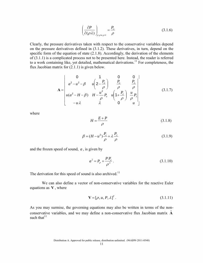
Clearly, the pressure derivatives taken with respect to the conservative variables depend on the pressure derivatives defined in (3.1.2). These derivatives, in turn, depend on the specific form of the equation of state (2.1.8). Accordingly, the derivation of the elements of (3.1.1) is a complicated process not to be presented here. Instead, the reader is referred to a work containing like, yet detailed, mathematical derivations.11 For completeness, the flux Jacobian matrix for (2.1.1) is given below.

uu

PuP

uPu

HHau

PPPuua

ee

ee

0

1

2

0010

22

22

)(A (3.1.7)

where

PEH

(3.1.8)

PPuH e )( 2 (3.1.9)

and the frozen speed of sound, a , is given by

22

ePPPa . (3.1.10)

The derivation for this speed of sound is also archived.11

We can also define a vector of non-conservative variables for the reactive Euler equations as V , where TPu ],,,[ V . (3.1.11) As you may surmise, the governing equations may also be written in terms of the non-conservative variables, and we may define a non-conservative flux Jacobian matrix A such that11


12

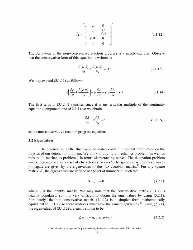
u

ua

u

u

00000

01000

ˆ2

A (3.1.12)

The derivation of the non-conservative reaction progress is a simple exercise. Observe that the conservative form of this equation is written as

rxt

)()( (3.1.13)

We may expand (3.1.13) as follows.

rx

utx

u

t

)( (3.1.14)

The first term in (3.1.14) vanishes since it is just a scalar multiple of the continuity equation (component one of 2.1.1), so we obtain

rx

ut

(3.1.15)

as the non-conservative reaction progress equation. 3.2 Eigenvalues The eigenvalues of the flux Jacobian matrix contain important information on the physics of our detonation problem. We think of any fluid mechanics problem (as well as most solid mechanics problems) in terms of interacting waves. The detonation problem can be decomposed into a set of characteristic waves.2 The speeds at which these waves propagate are given by the eigenvalues of the flux Jacobian matrix.12 For any square matrix A , the eigenvalues are defined as the set of numbers such that 0 IA (3.2.1) where I is the identity matrix. We may note that the conservative matrix (3.1.7) is heavily populated, so it is very difficult to obtain the eigenvalues by using (3.2.1). Fortunately, the non-conservative matrix (3.1.12) is a simpler form mathematically equivalent to (3.1.7), so these matrices must have the same eigenvalues.11 Using (2.3.1), the eigenvalues of (3.1.12) are easily shown to be },,,{ auuuau (3.2.2)


13

Note that u is an eigenvalue of multiplicity two, so there are two waves with speed u , i.e., the entropy and reaction progress waves both propagating at the flow velocity. The remaining two distinct eigenvalues au denote acoustic waves.12 The dynamics of the detonation process may be described through the interactions of characteristic waves, but to completely describe these waves, we must determine the eigenvectors for the detonation problem. 3.3 Eigenvectors In order to determine the characteristic waves for (2.1.1), we must determine the eigenvectors for the conservative Jacobian matrix (3.1.7). When we use the term eigenvector, in this case, we are referring to a right eigenvector.10

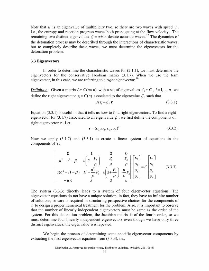
Definition: Given a matrix )( nnA C with a set of eigenvalues Ci , ni ,,1 , we define the right eigenvector )(ni Cr associated to the eigenvalue i such that iiiA rr (3.3.1) Equation (3.3.1) is useful in that it tells us how to find right eigenvectors. To find a right eigenvector for (3.1.7) associated to an eigenvalue , we first define the components of right eigenvector r . Let T),,,( 4321 r (3.3.2) Now we apply (3.1.7) and (3.3.1) to create a linear system of equations in the components of r .

4

3

2

1

4

3

2

1

22

22

0

1

2

0010

uu

PuP

uPu

HHau

PPPuua

ee

ee

)( (3.3.3)

The system (3.3.3) directly leads to a system of four eigenvector equations. The eigenvector equations do not have a unique solution; in fact, they have an infinite number of solutions, so care is required in structuring prospective choices for the components of r to design a proper numerical treatment for the problem. Also, it is important to observe that the number of linearly independent eigenvectors must be same as the order of the system. For this detonation problem, the Jacobian matrix is of the fourth order, so we must determine four linearly independent eigenvectors even though we have only three distinct eigenvalues; the eigenvalue u is repeated.

We begin the process of determining some specific eigenvector components by extracting the first eigenvector equation from (3.3.3), i.e.,


14

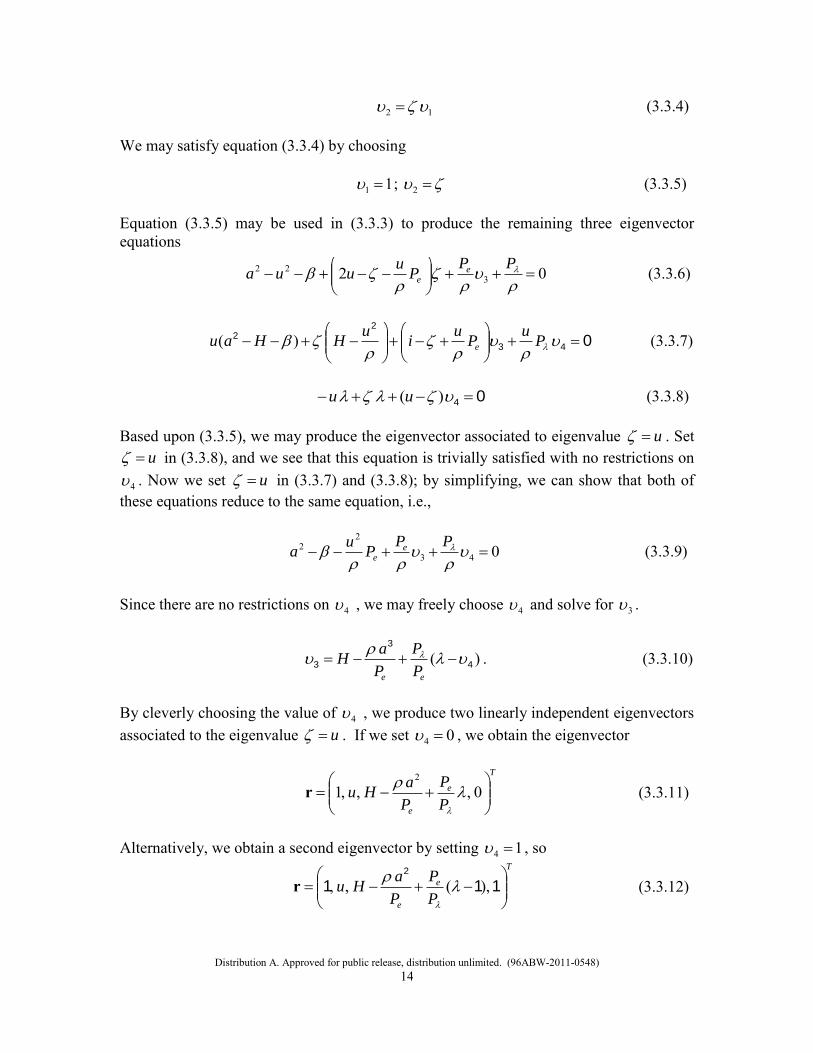
12 (3.3.4) We may satisfy equation (3.3.4) by choosing 11 ; 2 (3.3.5) Equation (3.3.5) may be used in (3.3.3) to produce the remaining three eigenvector equations

02 322

PP

Pu

uua ee (3.3.6)

043

22

P

uP

ui

uHHau e)( (3.3.7)

04 )(uu (3.3.8) Based upon (3.3.5), we may produce the eigenvector associated to eigenvalue u . Set

u in (3.3.8), and we see that this equation is trivially satisfied with no restrictions on

4 . Now we set u in (3.3.7) and (3.3.8); by simplifying, we can show that both of these equations reduce to the same equation, i.e.,

043

22

PP

Pu

a ee (3.3.9)

Since there are no restrictions on 4 , we may freely choose 4 and solve for 3 .

)( 4

3

3

ee P

P

P

aH . (3.3.10)

By cleverly choosing the value of 4 , we produce two linearly independent eigenvectors associated to the eigenvalue u . If we set 04 , we obtain the eigenvector

T

e

e P

P

P

aHu

0,,,1

2

r (3.3.11)

Alternatively, we obtain a second eigenvector by setting 14 , so

T

e

e P

P

P

aHu

111

2

),(,,

r (3.3.12)


15

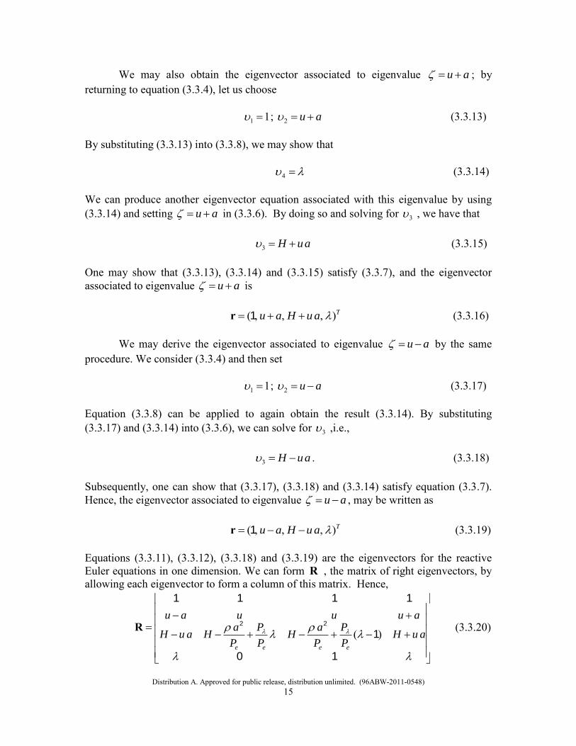
We may also obtain the eigenvector associated to eigenvalue au ; by returning to equation (3.3.4), let us choose 11 ; au 2 (3.3.13) By substituting (3.3.13) into (3.3.8), we may show that 4 (3.3.14) We can produce another eigenvector equation associated with this eigenvalue by using (3.3.14) and setting au in (3.3.6). By doing so and solving for 3 , we have that auH 3 (3.3.15) One may show that (3.3.13), (3.3.14) and (3.3.15) satisfy (3.3.7), and the eigenvector associated to eigenvalue au is TauHau ),,,( 1r (3.3.16) We may derive the eigenvector associated to eigenvalue au by the same procedure. We consider (3.3.4) and then set 11 ; au 2 (3.3.17) Equation (3.3.8) can be applied to again obtain the result (3.3.14). By substituting (3.3.17) and (3.3.14) into (3.3.6), we can solve for 3 ,i.e., auH 3 . (3.3.18) Subsequently, one can show that (3.3.17), (3.3.18) and (3.3.14) satisfy equation (3.3.7). Hence, the eigenvector associated to eigenvalue au , may be written as TauHau ),,,( 1r (3.3.19) Equations (3.3.11), (3.3.12), (3.3.18) and (3.3.19) are the eigenvectors for the reactive Euler equations in one dimension. We can form R , the matrix of right eigenvectors, by allowing each eigenvector to form a column of this matrix. Hence,

10

1

1111

22

auHP

P

P

aH

P

P

P

aHauH

auuuau

eeee

)(R (3.3.20)


16

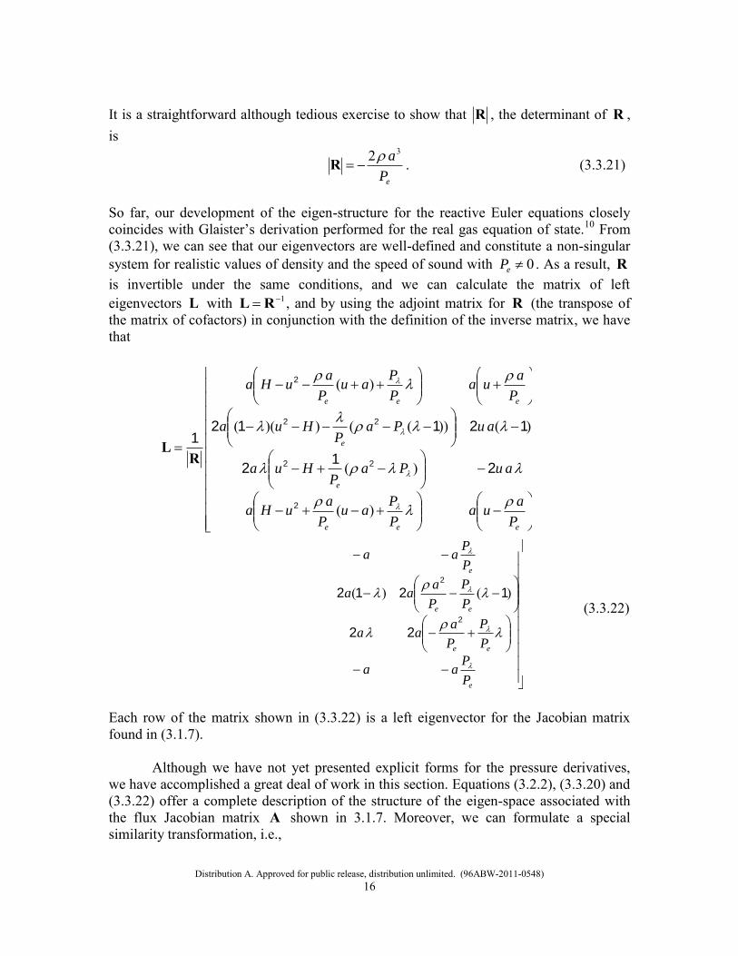
It is a straightforward although tedious exercise to show that R , the determinant of R , is

eP

a32R . (3.3.21)

So far, our development of the eigen-structure for the reactive Euler equations closely coincides with Glaister’s derivation performed for the real gas equation of state.10 From (3.3.21), we can see that our eigenvectors are well-defined and constitute a non-singular system for realistic values of density and the speed of sound with 0eP . As a result, R is invertible under the same conditions, and we can calculate the matrix of left eigenvectors L with 1RL , and by using the adjoint matrix for R (the transpose of the matrix of cofactors) in conjunction with the definition of the inverse matrix, we have that

eee

e

e

eee

P

aua

P

Pau

P

auHa

auPaP

Hua

auPaP

Hua

P

aua

P

Pau

P

auHa

)(

)(

)())(())((

)(

2

22

22

2

21

2

121121

RL

e

ee

ee

e

P

Paa

P

P

P

aaa

P

P

P

aaa

P

Paa

2

2

22

1212 )()( (3.3.22)

Each row of the matrix shown in (3.3.22) is a left eigenvector for the Jacobian matrix found in (3.1.7). Although we have not yet presented explicit forms for the pressure derivatives, we have accomplished a great deal of work in this section. Equations (3.2.2), (3.3.20) and (3.3.22) offer a complete description of the structure of the eigen-space associated with the flux Jacobian matrix A shown in 3.1.7. Moreover, we can formulate a special similarity transformation, i.e.,


17

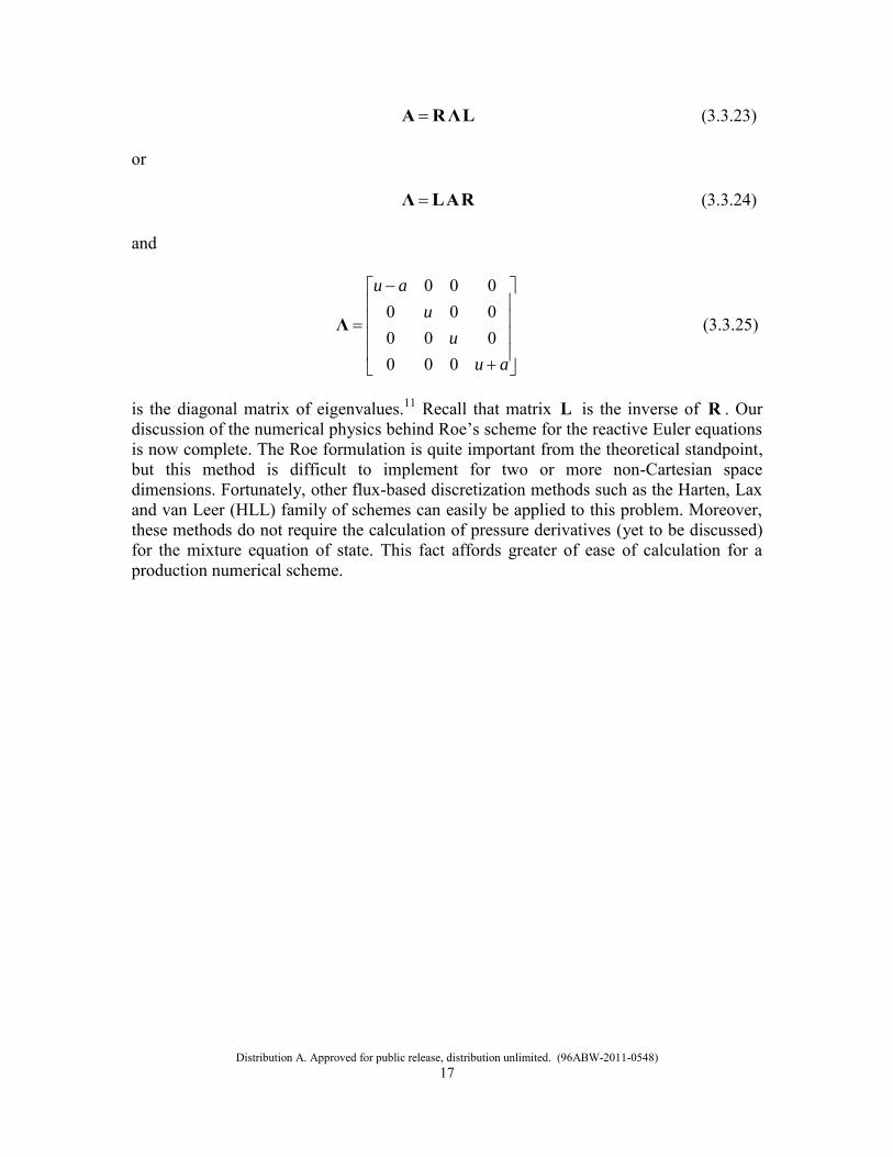
LΛRA (3.3.23) or RALΛ (3.3.24) and

au

u

u

au

000000000000

Λ (3.3.25)

is the diagonal matrix of eigenvalues.11 Recall that matrix L is the inverse of R . Our discussion of the numerical physics behind Roe’s scheme for the reactive Euler equations is now complete. The Roe formulation is quite important from the theoretical standpoint, but this method is difficult to implement for two or more non-Cartesian space dimensions. Fortunately, other flux-based discretization methods such as the Harten, Lax and van Leer (HLL) family of schemes can easily be applied to this problem. Moreover, these methods do not require the calculation of pressure derivatives (yet to be discussed) for the mixture equation of state. This fact affords greater of ease of calculation for a production numerical scheme.


18

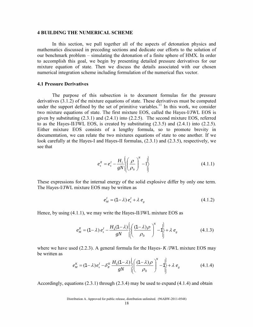
4 BUILDING THE NUMERICAL SCHEME In this section, we pull together all of the aspects of detonation physics and mathematics discussed in preceding sections and dedicate our efforts to the solution of our benchmark problem – simulating the detonation of a finite sphere of HMX. In order to accomplish this goal, we begin by presenting detailed pressure derivatives for our mixture equation of state. Then we discuss the details associated with our chosen numerical integration scheme including formulation of the numerical flux vector. 4.1 Pressure Derivatives The purpose of this subsection is to document formulas for the pressure derivatives (3.1.2) of the mixture equations of state. These derivatives must be computed under the support defined by the set of primitive variables.11 In this work, we consider two mixture equations of state. The first mixture EOS, called the Hayes-I/JWL EOS is given by substituting (2.3.1) and (2.4.1) into (2.2.5). The second mixture EOS, referred to as the Hayes-II/JWL EOS, is created by substituting (2.3.5) and (2.4.1) into (2.2.5). Either mixture EOS consists of a lengthy formula, so to promote brevity in documentation, we can relate the two mixtures equations of state to one another. If we look carefully at the Hayes-I and Hayes-II formulas, (2.3.1) and (2.3.5), respectively, we see that

1

0

1

N

I

s

II

sgN

Hee

(4.1.1)

These expressions for the internal energy of the solid explosive differ by only one term. The Hayes-I/JWL mixture EOS may be written as g

I

s

I

M eee )(1 (4.1.2) Hence, by using (4.1.1), we may write the Hayes-II/JWL mixture EOS as

g

N

I

s

II

M egN

Hee

1

111

0

1 )()()( (4.1.3)

where we have used (2.2.3). A general formula for the Hayes- K /JWL mixture EOS may be written as

g

N

K

II

I

s

K

M egN

Hee

1

111

0

1 )()()( (4.1.4)

Accordingly, equations (2.3.1) through (2.3.4) may be used to expand (4.1.4) and obtain


19

111

11

111

0

1

02

2

1

1

5

1

0

40

N

K

II

N

NK

M

gN

H

eQR

RB

R

RA

ttDPe

)()(

)(ˆ

expˆˆ

expˆ

)()(

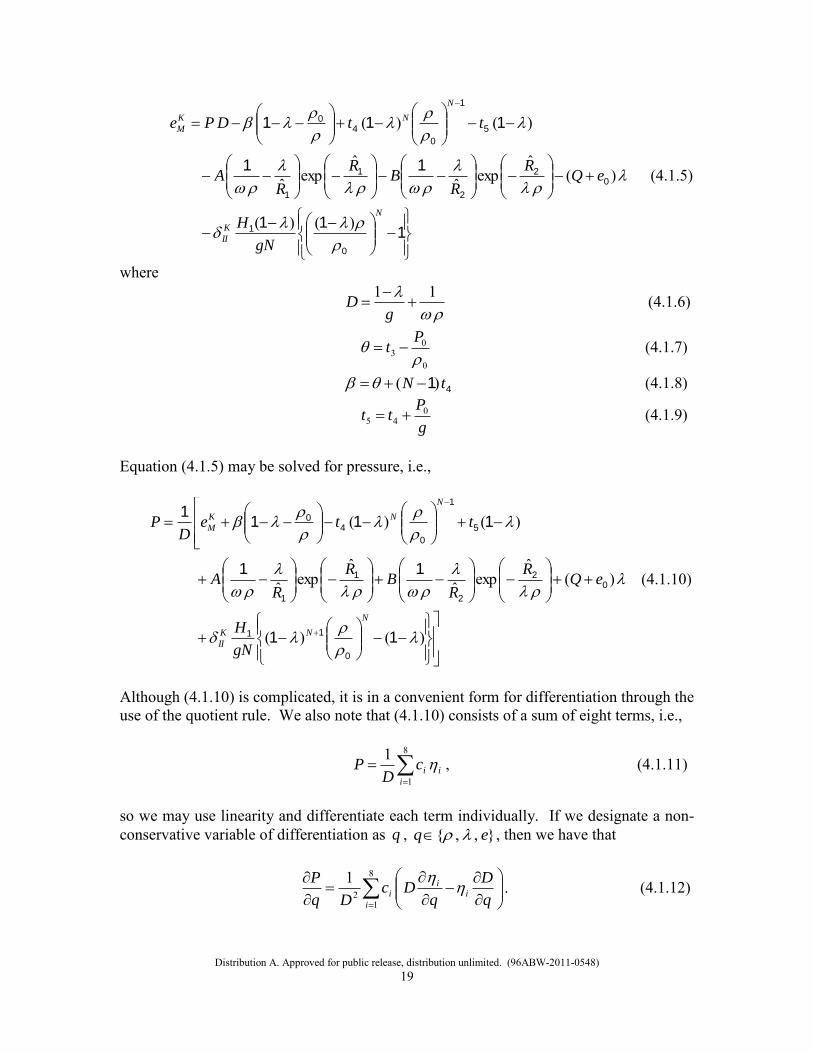
(4.1.5)

where

11

gD (4.1.6)

0

03

Pt (4.1.7)

41 tN )( (4.1.8)

g

Ptt 0

45 (4.1.9)

Equation (4.1.5) may be solved for pressure, i.e.,

)()(

)(ˆ

expˆˆ

expˆ

)()(

11

11

1111

0

11

02

2

1

1

5

1

0

40

N

NK

II

N

NK

M

gN

H

eQR

RB

R

RA

tteD

P

(4.1.10)

Although (4.1.10) is complicated, it is in a convenient form for differentiation through the use of the quotient rule. We also note that (4.1.10) consists of a sum of eight terms, i.e.,

8

1

1i

iicD

P , (4.1.11)

so we may use linearity and differentiate each term individually. If we designate a non-conservative variable of differentiation as q , },,{ eq , then we have that

8

12

1i

ii

iq

D

qDc

Dq

P

. (4.1.12)


20

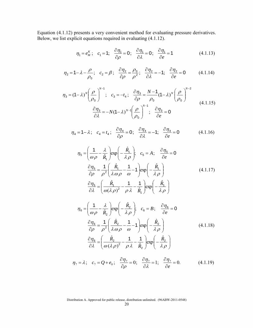
Equation (4.1.12) presents a very convenient method for evaluating pressure derivatives. Below, we list explicit equations required in evaluating (4.1.12).

1001 11111

eceK

M

;;;; (4.1.13)

011 22

2

022

0

2

ec

;;;; (4.1.14)

01

11

1

3

1

0

13

2

00

343

1

0

3

eN

Ntc

N

N

N

N

N

N

;)(

)(;;)( (4.1.15)

0101 444444

etc

;;;; (4.1.16)

1

1

2

15

11

2

5

55

1

1

5

11

111

01

R

R

R

RR

eAc

R

R

êxpˆ)(

ˆ

êxp

ˆ

;;ˆ

expˆ

(4.1.17)

2

2

2

26

22

2

6

66

2

2

6

11

111

01

R

R

R

RR

eBc

R

R

êxpˆ)(

ˆ

êxp

ˆ

;;ˆ

expˆ

(4.1.18)

.0;1;0;; 777077

eeQc

(4.1.19)


21

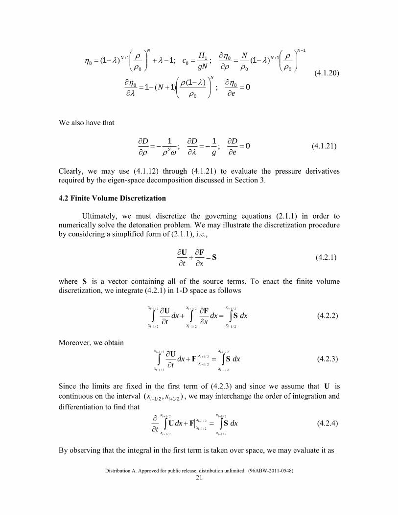
01

11

111

8

0

8

1

0

1

0

818

0

1

8

eN

N

gN

Hc

N

N

N

N

N

;)()(

)(;;)( (4.1.20)

We also have that

011

2

e

D

g

DD ;;

(4.1.21)

Clearly, we may use (4.1.12) through (4.1.21) to evaluate the pressure derivatives required by the eigen-space decomposition discussed in Section 3. 4.2 Finite Volume Discretization Ultimately, we must discretize the governing equations (2.1.1) in order to numerically solve the detonation problem. We may illustrate the discretization procedure by considering a simplified form of (2.1.1), i.e.,

SFU

xt (4.2.1)

where S is a vector containing all of the source terms. To enact the finite volume discretization, we integrate (4.2.1) in 1-D space as follows

2/1

2/1

2/1

2/1

2/1

2/1

i

i

i

i

i

i

x

x

x

x

x

x

dxdxx

dxt

SFU (4.2.2)

Moreover, we obtain

2/1

2/1

2/1

2/1

2/1

2/1

i

i

i

i

i

i

x

x

x

x

x

x

dxdxt

SFU (4.2.3)

Since the limits are fixed in the first term of (4.2.3) and since we assume that U is continuous on the interval ),( // 2121 ii xx , we may interchange the order of integration and differentiation to find that

2/1

2/1

2/1

2/1

2/1

2/1

i

i

i

i

i

i

x

x

x

x

x

x

dxdxt

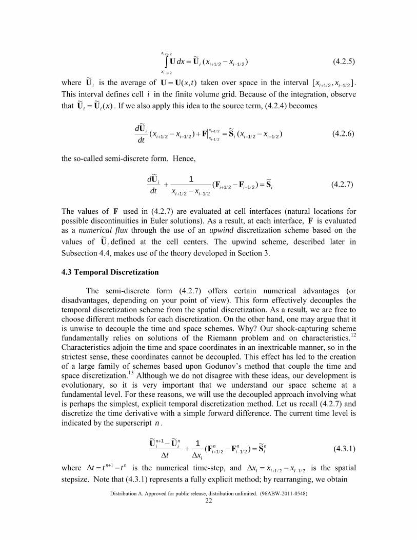
SFU (4.2.4)

By observing that the integral in the first term is taken over space, we may evaluate it as


22

)(~//

/

/

2121

21

21

iii

x

x

xxdxi

i

UU (4.2.5)

where iU~ is the average of ),( txUU taken over space in the interval ],[ // 2121 ii xx . This interval defines cell i in the finite volume grid. Because of the integration, observe that )(~~

xii UU . If we also apply this idea to the source term, (4.2.4) becomes

)(~)(~

/////

/21212121

21

21

iii

x

xiii xxxx

dt

d i

i

SFU (4.2.6)

the so-called semi-discrete form. Hence,

iii

ii

i

xxdt

d SFFU ~)(~

////

2121

2121

1 (4.2.7)

The values of F used in (4.2.7) are evaluated at cell interfaces (natural locations for possible discontinuities in Euler solutions). As a result, at each interface, F is evaluated as a numerical flux through the use of an upwind discretization scheme based on the values of iU~ defined at the cell centers. The upwind scheme, described later in Subsection 4.4, makes use of the theory developed in Section 3. 4.3 Temporal Discretization The semi-discrete form (4.2.7) offers certain numerical advantages (or disadvantages, depending on your point of view). This form effectively decouples the temporal discretization scheme from the spatial discretization. As a result, we are free to choose different methods for each discretization. On the other hand, one may argue that it is unwise to decouple the time and space schemes. Why? Our shock-capturing scheme fundamentally relies on solutions of the Riemann problem and on characteristics.12 Characteristics adjoin the time and space coordinates in an inextricable manner, so in the strictest sense, these coordinates cannot be decoupled. This effect has led to the creation of a large family of schemes based upon Godunov’s method that couple the time and space discretization.13 Although we do not disagree with these ideas, our development is evolutionary, so it is very important that we understand our space scheme at a fundamental level. For these reasons, we will use the decoupled approach involving what is perhaps the simplest, explicit temporal discretization method. Let us recall (4.2.7) and discretize the time derivative with a simple forward difference. The current time level is indicated by the superscript n .

n

i

n

i

n

i

i

n

i

n

i

xtSFFUU ~)(

~~//

2121

1 1 (4.3.1)

where nn ttt 1 is the numerical time-step, and 2/12/1 iii xxx is the spatial stepsize. Note that (4.3.1) represents a fully explicit method; by rearranging, we obtain


23

xt

n

i

n

in

i

n

i

n

i2/12/11 ~~~ FFSUU (4.3.2)

Basically, equation (4.3.2) implements the Euler time integration method.14 The only numerical stability control we place on (4.3.2) involves a restriction on the time-step t . This restriction is enforced through a Courant-Friedrichs-Lewy (CFL) criterion. We apply a factor of 0.5 to the new predicted time-step given by

ii

i

ii

pred

au

xt

max1min (4.3.3)

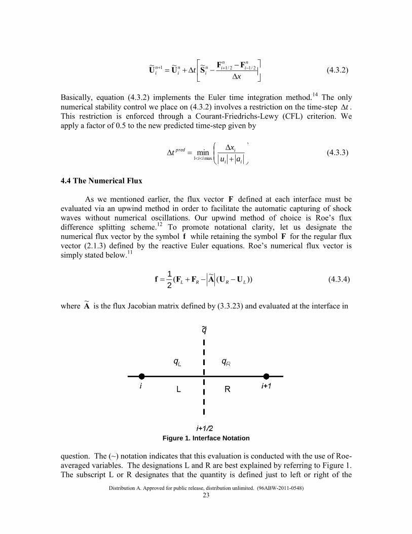
4.4 The Numerical Flux As we mentioned earlier, the flux vector F defined at each interface must be evaluated via an upwind method in order to facilitate the automatic capturing of shock waves without numerical oscillations. Our upwind method of choice is Roe’s flux difference splitting scheme.12 To promote notational clarity, let us designate the numerical flux vector by the symbol f while retaining the symbol F for the regular flux vector (2.1.3) defined by the reactive Euler equations. Roe’s numerical flux vector is simply stated below.11

))(~( LRRL UUAFFf 2

1 (4.3.4)

where A~ is the flux Jacobian matrix defined by (3.3.23) and evaluated at the interface in

Figure 1. Interface Notation

question. The (~) notation indicates that this evaluation is conducted with the use of Roe-averaged variables. The designations L and R are best explained by referring to Figure 1. The subscript L or R designates that the quantity is defined just to left or right of the


24

interface, respectively. In Figure 1, the interface is located at 2/1ix between cell i and cell 1i . Why would the left and right interface values of some property differ? The answer is very simple. Remember that we stated earlier that our method involves solutions of the Riemann problem. These solutions admit discontinuities, e.g., shock waves. Hence, by the nature of a discontinuity, the properties taken to the left and the right of an interface differ. In the simplest view, we can say that the properties to the left of the interface taken on the values defined in cell i ; it follows that the properties to the right of the interface take on the values defined in cell 1i . This means of selecting the left and right interface values renders first-order accuracy on uniform meshes. There are other ways to define these upwind values. A higher order method is discussed in a later subsection. Our Roe averages are computed from these upwind (L and R) variables. The Roe average constitutes the physically correct representation of an average at a discontinuity conforming to the basic ideas of flux difference splitting.15 A mathematically lengthy derivation is required to produce Roe’s formulas, so we merely state the results.10

RL ~ (4.3.5)

RL

RRLL uuu

~ (4.3.6)

RL

RRLL HHH

~ (4.3.7)

RL

RRLL eee

~ (4.3.8)

RL

RRLL

~ (4.3.9)

2~

21~~~~

ueHP (4.3.10)

22

~~~~~

ePPPa (4.3.11)

One may note that (3.3.20) through (3.3.22), (3.3.25) and (4.3.11) require Roe-averaged pressure derivatives. Recall that explicit formulas for these derivatives are presented in (4.1.12) through (4.1.20). The derivatives are presented in terms of the primitive variables, so we claim that Roe-averaged values of the pressure derivatives may be


25

obtained by simply evaluating these formulas for the Roe-averaged variables presented in (4.3.5) through (4.3.10). In practice, this procedure seems to work well. We may now address the practical evaluation of the numerical flux vector as it is defined in (4.3.4). The vectors LF and RF are the standard Euler flux vectors (2.1.3) evaluated for the upwind conservative variables LU and RU (or primitive variables Rq and Lq ), respectively. The remaining term )(~

LR UUA (4.3.12)

is denoted as the numerical viscosity expression. The difference between the conservative variables left and right of the interface may be easily evaluated through the use of (2.1.2). A~ may be evaluated as follows.

LΛRA ~~~~ (4.3.13)

where the (~) notation indicates that all of the entries in the matrices are calculated with the use of averaged variables. The matrix Λ~ is created by taking the absolute value of

each element of Λ~ , the diagonal matrix of eigenvalues. Finally, (4.3.12) is computed by a series of simple matrix-matrix and matrix-vector multiplications; (4.3.4) is easily evaluated by using vectors sums. 4.5 A Higher-Order Scheme The scheme described in the preceding subsection is only accurate to the first order, and it is highly dissipative, a detriment to the sharp resolution of detonation waves. In this subsection, we briefly describe an enhancement to the first order scheme that is third-order accurate on uniform grids. As you may have concluded, the left and right interface values are constructed from the cell-center values to the left and right of the interface, respectively. To increase the order of accuracy for the scheme, we instead reconstruct the interface values using interpolating polynomials involving more than one cell-center value. One way to apply this idea is through the use of a Monotone Upwind Scheme for Conservation Laws (MUSCL).12 The equations for the left and right interface variables are provided below for the interface located at 2/1i . Consider the primitive variable q , ,,, Puq .

)()())(()( 1211

111

4

1ii

L

iiLiL qqr

qqrqq

(4.4.1) where 3/1 to achieve third-order accuracy, and


26

21

1

ii

iiL

qq

qqr . (4.4.2)

is a function designed to serve as a non-limiter limiter. In every case, our interpolated data must be monotone; otherwise, the interpolation procedure will result in the formation of non-physical oscillations in the numerical solution.12 The nonlinear limiter is designed to maintain the monotonicity of smooth sections of data when interpolated to high order. We have chosen the Van Albada limiter for use in this problem, i.e.,

2

2

1 r

rrr

)( (4.4.3)

The right interface variable is given by

)()())(()( 11

111

4

1ii

R

iiRiR qqr

qqrqq (4.4.4)

For this expression, the ratio used by the limiter is defined as

ii

iiR

qq

qqr

1

1 (4.4.5)

Equations (4.4.1) through (4.4.5) cannot be implemented without due cognizance. The left interpolant involves cell-center values located at 2i , 1i and i . As a result, we must ensure that 0211 )()( iiii qqqq (4.4.6) Otherwise, the cell-center data is non-monotone, and the interface values must be set to the first-order values

iR

iL

qq

qq

1 (4.4.7)

in order to properly smooth the solution. For the right interpolant, we must ensure that 011 )()( iiii qqqq (4.4.8) or we must use the first-order interpolation values (4.4.7). In addition, after the criteria (4.4.6) and (4.4.8) are satisfied, we are required to limit on the ratios (4.4.2) and (4.4.5). Based on the data, these ratios may become undefined, so the limiter function (4.4.3) must be modified ensure that its value always remains finite. If this interpolation strategy is used properly, the Roe algorithm becomes a high-resolution flux difference splitting scheme.


27

4.6 Boundary Conditions In most cases, we cannot solve partial differential equations without applying boundary conditions. Even for our simple detonation problem cast in one dimension, we must apply boundary conditions at 0x (the center of the sphere) and at MAXxx (the outer surface of the sphere). At the center of the sphere, we enforce fully reflective boundary conditions through the use of a ghost cell installed at 0i , i.e.,

1

1

1

1

10

ee

PP

uu

0

0

0

0

(4.5.1)

We have assumed that the first flow field cell adjacent to this boundary has the index

1i . At the outer surface of the sphere, we apply extrapolated boundary conditions to mimic a supersonic outflow. We implement this condition by installing a ghost cell at

MAXii . We set conditions in this cell as follows.

1-IMAXIMAX

1-IMAXIMAX

1-IMAXIMAX

1-IMAXIMAX

1-IMAXIMAX

ee

PP

uu

(4.5.2)

Boundary conditions (4.5.1) and (4.5.2) function well for the detonation of a finite spherical mass of HMX.


28

5 PARTICLE MOTION

In this section, we extend our discussion beyond the application of numerical detonation literature cited thus far. Given the level of interest in Multiphase Blast Explosives (MBX), it is desirable to incorporate solid particles into our detonation programming. This effort is new, so our treatment of solid particles is limited, to a certain extent. Still, our particles have realistic mass and finite radii. They are driven by the detonation through the use of Lagrangian laws of motion. Our particle algorithms have only three major limitations: (i) The particle collection exists in the diffuse limit. Particles are assumed not to interact with one another. (ii) Particles are assumed to exist as rigid spheres. The do not deform or change phase during the detonation event. (iii) This model is restricted to one dimension. We can only establish initial particle positions along a single ray. Based on these assumptions, we can investigate the efficacy of this model in predicting the post-detonation conditions for a mass of solid HMX loaded with particles. 5.1 Coupling Terms We may now discuss the coupling terms (source terms) for particles presented in equations (2.1.1) and (2.1.6). sF and sQ have relatively simple descriptions. sF represents the transfer of momentum between the gas phase and the particle phase while

sQ represents the similar transfer of thermal energy. For spherical particles, these terms may be written in a simple form.6 Assume that the total number of particles is pN .

dt

durF

p

pp

N

p

s

p

3

1 34

(5.1.1)

pN

p

ppps TTrhQ1

24 )~( (5.1.2)

where p , pr and pu are the solid density, radius and velocity of the thp particle,

respectively. Therefore, dtdu p / is the acceleration of the thp particle. Also, T~ is the

temperature of the gas phase at the surface of the particle, and pT is the particle

temperature. Actually, T~ is the Favre-filtered temperature; this filtering operation is used to take the presence of turbulence into account. Our simulation is non-viscous, so we simply set T~ equal to the gas phase temperature T . The parameter ph is the heat transfer coefficient that governs the transfer of thermal energy at the particle/fluid interface. In


29

general, ph is experimentally determined. By specifying (5.1.1) and (5.1.2), we can accurately describe the coupling between the gas and particulate phases. Of course, these equations only apply to particles of fixed mass. Additional terms (including mass conservation) must be specified for particles that react with the gas phase. 5.2 Particle Laws of Motion The detonation physics algorithms incorporate discrete, finite-mass particles, so we apply Lagrangian equations for tracking the movement of particles. Let px designate

the radial coordinate of the thp particle. Then we have that

p

pu

dt

dx (5.2.1)

The particle velocity pu must be determined from the evolution equation given by a model. We have two alternatives for this model; the first is called the “Spray Model” which may be described as follows.6

)(Re

p

pp

pDpuu

r

C

dt

du

216

3

(5.2.2)

where the particle Reynolds number pRe is defined as

p

p

p uur

2Re (5.2.3)

The drag coefficient for the particle DC is conveyed by the “Spray Drag Law”, i.e.,

1000440

10006

124

32

p

p

p

p

DC

Re.

ReRe

Re

/

(5.2.4)

, and u are the density, dynamic viscosity and velocity of the gas phase in the vicinity of the particle. This model is not appropriate for detonation problems, but it still serves well for testing. For the problem of a detonation with solid inclusions, we apply a high speed gas flow model originally developed for solid rocket motors.


30

The high speed gas flow model was developed for the multiphase flow field created by the burn of porous, powdered explosive material.16 In this case, the particle acceleration is given by

)( pp

p

Dppuuuu

m

Cd

dt

du

2

8. (5.2.5)

In order to maintain our notation consistent with the literature, (5.2.5) is written in terms of the particle diameter pd instead of the radius. Also, pm is the mass of the thp particle. This high speed drag law provides the drag coefficient through a more complicated calculation. First, we calculate a “Mach-zero” drag coefficient, 0DC , i.e.,

450

450080370

080450

080

22

22212

21

0

.

...

).().(

.

C

CC

C

CD

(5.2.6) where pRe is calculated by using (5.2.3), and

42.0Re

4.4Re24

1 pp

C (5.2.7)

p

CRe

15075.13

4

1

2

12

. (5.2.8)

In (5.2.6) and (5.22.8), we have introduced two new parameters 1 and 2 ; they are the volume concentrations of the gas and particle phases, respectively. These parameters require interpretation when considering the detonation problem. At the outset of the problem, the solid explosive has not been detonated, so there is no gas phase at this point. The best course of action is to compute the initial values of 1 and 2 based upon the volume of the solid explosive and the volume of particles. Since we are not simulating details of the shock interaction with metal particles, we calculate 1 and 2 on this basis of the initial calculation and maintain them fixed for the duration of the detonation. We must then calculate a final value of DC based on a Mach correction.17 This correction exists due to the natural variation in the drag coefficient with Mach number. If we do not wish to implement a drag correction, then we set 0DD CC ; otherwise the corrected value of DC may be calculated from


31

63.40

427.0exp1M

CC DD , (5.2.9)

where

a

uuM

p . (5.2.10)

By using the particle velocities provided by (5.2.2) though (5.2.4) or (5.2.5) through (5.2.10), we may integrate (5.2.1) to determine the track of each particle through space during the detonation.


32

6 RESULTS

From the start of this effort, several versions of our current numerical detonation computer code have been developed by the author. The purpose of this section is to present some of the results produced for typical problems. Specifically, we discuss three results. The first set of results is intended to show that our detonation program is functioning properly and producing physically correct solutions. In a second calculation, we address the numerical detonation of a spherical mass of pure HMX. For this problem, we have computed results by using both the Hayes-I and Hayes-II equations of state for the solid explosive combined with the JWL EOS for the detonation products. Finally, we discuss the results for the detonation of a spherical mass of HMX loaded with steel particles. 6.1 Simple Plane Wave Detonation This test problem, described in Reference 2, is used to show whether or not the flux difference splitting scheme is working properly. In this case, we endeavor to solve a Deflagration to Detonation Transition (DDT) problem in one dimension. Both the explosive and the detonation products are modeled by using the calorically perfect gas EOS. The associated mixture EOS is given as

QP

e

)( 1

(6.1.1)

As discussed in Section 4, we apply fully reflective boundary conditions at 0x and extrapolation conditions at MAXxx . For this problem, we use the reaction rate expression

P

Ekr aexp)(1 (6.1.2)

where (6.1.2) is in Arrhenius form; k is the reaction rate constant, and aE is a parameter that behaves like an activation energy. The one-dimensional domain is defined in

120 x . Also, we have that 10aE ; 50Q ; 4.1 , and 7k . The problem is initialized with 0u ; 0P , and 0 everywhere.2 The initial density distribution is given by

12031

12

xx

x ,)exp(

)( . (6.1.3)

This density distribution initiates the reaction in the region near 0x by boosting the reaction rate term.


33

Figure 2. Problem 1 Detonation Field Density, Time = 3.0

Figure 3. Problem 1 Detonation Field Velocity, Time = 3.0


34

Figure 4. Problem 1 Detonation Field Pressure, Time = 3.0

Figure 5. Problem 1 Detonation Field Reaction Progress Variable, Time = 3.0

This problem does not possess an “exact” solution, but Xu et al. have obtained a

fully converged numerical solution using a mesh consisting on 3200 cells.2 This problem provides an excellent test detonation physics algorithms. Accordingly, we have generated three numerical solutions on grids comprised of 200, 800 and 3200 cells, respectively. The numerical solutions for density, velocity, pressure and the reaction progress variable are provided in Figures 2 through 5, respectively, at the dimensionless time 3.0. In each figure, solution plots are color-coded to correspond to the mesh used. The behavior shown in each plot agrees quite well with archived plots.2 We have observed only one anomaly in our solutions. Strangely enough, on the mesh consisting of only 200 cells, there are noticeable oscillations in the reaction progress variable. These oscillations dissipate with increasing mesh density. The explanation for this behavior is not immediately evident. In some of our solutions, the reaction progress variable has been observed to hunt between the solid and gaseous equations of state. In fact, this variable is


35

very sensitive and couples strongly to the reaction rate. We apply no post-solution filtering to this variable. Secondly, we are using a weak time integration scheme with poor numerical stability performance. The oscillations become less prevalent with increasing grid density, so the space scheme may be compensating for the time scheme. This phenomenon bears further investigation as this work continues. We will also re-examine the nonlinear limiter coding. Nevertheless, our converged solution agrees well with the converged archival solution.2

6.2 Detonation of Pure HMX This problem is intended to demonstrate our computer code’s capability for simulating the detonation of a sphere of pure HMX. This problem permits a test of our discretization of the geometric source term found in the reactive Euler equations (2.1.1) and (2.1.4). It also represents our first attempt at capturing the physics of a realistic detonation event. In this case, we address the detonation of sphere of solid HMX with a radius of 4.5 cm. The radius of the sphere is divided into 800 cells. Figure 6 shows the density, velocity, pressure and reaction progress variables for the numerical solution at three microseconds (μs) detonation elapsed time. As you can see, the Von Neumann spike is clearly resolved in this solution as is the Taylor wave. Moreover, the Chapman-Jouquet pressure is captured at the experimentally obtained value of 42 GPa. Also, the numerical detonation velocity has a value of 1.02 cm/μs which is very close to the experimentally obtained value of 0.911 cm/μs.21 Of course, the experimental value is generally taken from tests that mimic plane wave detonation conditions. As a result, we expect to calculate a different value for the spherical detonation problem. Overall, the results agree very closely with the archival data. We have also solved this same problem by using the Hayes-II/JWL mixture EOS. The results of this analysis are given in Figure 7. It is interesting to observe that the Taylor wave is captured in this solution even more smoothly than it was in the preceding case. The more complex Hayes-II EOS may actually offer greater stability when used in the mixture EOS. This numerical solution also offers excellent comparisons with the Chapman-Jouquet pressure and detonation velocity for HMX. Both mixture equations of state show that the detonation reaction occurs in a nearly instantaneous manner. As you can see, the reaction progress variable changes in a nearly discontinuous manner at the detonation front. In either case, our computer programming captures the appropriate physics for the detonation, and it renders a wide array of physical data (far more than is shown here).


36

Figure 6. Numerical detonation solution Hayes-I/JWL in HMX at 3 μs. Horizontal axis is distance in meters.

Figure 7. Numerical detonation solution Hayes-I/JWL in HMX at 3 μs. Horizontal axis is distance in meters.


37

6.3 Detonation of HMX Containing Metal Particles This test case is the final detonation problem addressed by this report. We consider the detonation of a spherical mass of HMX loaded with a radial distribution of steel particles. The mass of the HMX sphere remains the same as is used for the preceding problem, and we still have 800 finite volume cells defined along the charge radius. For this example, we have placed ten particles, at uniform spacing, along the charge radius. The particles each have a radius of 463 μm and a material density of 7860 kg/m3. We assume the gas viscosity has a value of 1.7x10-5 kg/(m.s). Furthermore, in this simulation study, we have applied the high speed flow drag law. The results for particle locations are presented in Figure 8 while the plot of particle velocities is given in Figure 9. The particle tracks shown in Figure 8 clearly indicate the passage of the detonation wave. For particles farther away from the charge center, the particle tracks show changes in slope at progressively larger times. The sudden change in track slope concurs with the nearly discontinuous change seen in the particle velocity traces shown in Figure 9. Also, in Figure 9, the effect of the drag law can clearly be seen as the particle velocities rise rapidly in the wake of the detonation wave then fall quickly under the action of drag in the region behind the wave. We have also applied the Mach correction to the rocket drag law. In the velocity trace for the particle closest to the charge center, we can see the velocity begin to level off at 4.5 μs. Available data indicates that the calculated terminal velocity at or near 375 m/s is an acceptable value. This simulation does not include thermal effects since we are still in the process of completing our detonation products EOS.

Figure 8. Radial locations for steel particles embedded in a mass of detonating HMX


38

Figure 9. Radial velocities for steel particles embedded in a detonating mass of HMX


39

7 CONCLUSIONS In this report, we have presented the governing equations for the direct numerical simulation of the detonation of a solid explosive material. Proper equations of state have been discussed for both the solid explosive material and for the gaseous detonation products. From these equations of state, we have developed a mixture equation of state relating the specific internal energy for the detonation to the thermodynamic pressure. The resulting computer program has been tested on an archival detonation problem for the purpose of comparison. We have presented results for the detonation of a spherical mass of pure HMX. More importantly, we have incorporated particle tracking algorithms within the programming. As a result, the code can now explosively drive particles under the action of a detonation wave with coupling to a drag law. This mechanism allows the code to simulate the detonation of a Multiphase Blast Explosive in the diffuse limit of particle loading. We have built drag laws for both spray and high speed gas flow drag law into the code. For a test problem, we have simulated the detonation of a mass of HMX loaded with a radial distribution of steel particles. The trend in post-detonation velocities of these particles meet our expectations. 8 RECOMMENDATIONS During the months ahead, detonation physics algorithms are scheduled for implementation in LESLIE3D. The development of the present work has been a learning experience accompanied by a large number of difficulties, especially in the implementation of Roe’s flux difference splitting scheme. A first recommendation is that the HLL family of schemes be used instead. These schemes are more robust and do not require the use of pressure derivatives. Also, these schemes already operate well inside of LESLIE3D. The detonation physics solver will also benefit from the interface tracking scheme already coded into LESLIE3D. Clearly, the governing equation differ at the interface between the condensed explosive and the surrounding gas field. This situation necessitates an interface to maintain code stability. The detonation physics algorithms discussed here must be adapted for curvilinear coordinates in three dimensions. For HLL flux forms, this process should not be difficult. The author has already done some work in this area. However, the pressure and specific volume (or density) closures associated with the mixture equation of state do require attention. The Gas-Interpolated Stewart-Prasad-Asay (GISPA) method requires these closures to address the multiphase physics of detonation. There is no unique set of closures available for this process, but the chosen closures must be carefull accomplished. Some difficulty has been encountered in the use of the specific volume closure (due to Xu), and this difficulty should be investigated and resolved. The Hayes equation of state for the solid explosive is an older relationship that characterizes very few explosives. The Mie-Gruneisen equation of state characterizes many more explosive materials. That is to say, there is data available. However, the


40

mixture equation of state must be rederived for the Mie-Gruneisen formulation. It may be combined with the JWL adiabat for the detonation products, or with another real gas state equation. The “Wide-Ranging” detonation equation of state may also be implemented.4

Ultimately, the particle phase algorithms discussed here must be rewritten for dense phase fields. The detonation of a condensed explosive with solid inclusions is a dense phase problem. Also, the computer program is currently not properly written even in the diffuse limit as regards the nonhomogeneous source terms. The integration scheme should be changed to reflect the use of Strang splitting.1 That is to say, the spatial integration scheme should be advanced in separate step from the nonhomogeneous terms. For the latter step, the integration should be conducted in the temporal manner at each grid cell just like an initial value problem. REFERENCES 1. Strang, G., “On the construction and comparison of difference schemes”, SIAM J.

Numer. Anal., Vol. 5, No. 3, pp. 506-517, 1968. 2. Xu, S., Aslam, T. and Stewart, D.S., “High resolution numerical simulation of ideal and non-ideal compressible reacting flows with embedded internal boundaries”, Combust. Theory Modeling, Vol. 1, pp. 113-142, 1997. 3. Bdzil, J.B., Stewart, D. S. and Jackson, T.L., “Program burn algorithms based on detonation shock dynamics: Discrete approximations of detonation flows with discontinuous front models”, Journal of Computational Physics, Vol. 174, No. 2, pp. 870-902, 2001. 4. Wescott, B.L., On Detonation Diffraction in Condensed Phase Explosives, Doctoral Dissertation, University at Illinois at Urbana-Champaign, 2001. 5. Stewart, D.S., “Tools for Design of Advanced Explosive Systems and Other Investigations on Ignition and Transient Detonation”, Final Report on a Grant from the U.S. Air Force Research Laboratory Munition Directorate to the University of Illinois, 2005. 6. Chen, K.H. and Shuen, J.S., “A Coupled Multi-Block Solution Procedure for Spray Combustion in Complex Geometries”, AIAA Paper 93-0108, American Institute for Aeronautics and Astronautics, 31st Aerospace Sciences Meeting and Exhibit, January 1993. 7. Stewart, D.S., Electronic Communication, 2006. 8. Hayes, D.B., “A Pnt Detonation Criterion From Thermal Explosion Theory”, Sixth Symposium (International) on Detonation, Pasadena, California, 1976.


41

9. Davis, W.C., “Complete equation of state for unreacted solid explosive”, Combustion

and Flame, Vol. 120, pp. 399-403, 2000. 10. Glaister, P., “An approximate linearised Riemann solver for the Euler equations for real gases”, Journal of Computational Physics, Vol. 74, pp. 382-408, 1988. 11. Nance, D.V., “Flux Difference Splitting Algorithms for Real Gas Mixtures”, Technical Memorandum, Munitions Directorate, Air Force Research Laboratory, March 2006. 12. Hirsch, C., Numerical Computation of Internal and External Flows, Vol. 2, John Wiley & Sons, New York, 1991. 13. Collela, P. and Woodward, P.R., “The piece-wise parabolic method for gas-dynamical simulations”, Journal of Computational Physics, Vol. 54, pp. 174-201, 1984. 14. Burden, R.L., Faires, J.D. and Reynolds, A.C., Numerical Analysis, 2nd Ed., Prindle, Weber & Schmidt, Boston, 1981. 15. Roe, P.L., “Approximate Riemann solvers, parameter vectors and difference schemes”, Journal of Computational Physics, Vol. 43, p. 357, 1981. 16. Akhatov, I.S. and Vainshtein, P.B., “Transition of porous explosive combustion into detonation”, Combustion, Explosion and Shock Waves, Vol. 20, No.1, pp. 63-70, 1984. 17. Carlson, D.J. and Hoglund, R.F., “Particle drag and heat transfer in rocket nozzles”, AIAA Journal, Vol. 2, No. 11, pp. 1980-1984, 1964.


42

APPENDIX A SOURCE CODE Instructions: The source code that follows has been developed over a period of six years, but in a sporadic manner, as time has permitted. FORTRAN 77 is used throughout the computer program, and an in-line coding structure has been used. The programming is designed for research and is thus rather crude. The initial conditions (shock-based initiation) are all rigidly coded. Different initiation options exist, but they must be enabled or disabled by commenting. The detonation reaction rate laws are treated in the same way. The desired reaction rate law must be commented in for the initial conditions and for the first and second time step segments of the solver. The calorically perfect gas and Jones-Wilkins-Lee test problems are also activated or deactivated by commenting in/out code segments. This computer program is written for standard explosives like HMX for which we have plenty of data. Especially for the Hayes equation of state, a great deal of data input is required. This data is simply entered directly into the source code. This statement is also true as pertains to the Jones-Wilkins-Lee detonation product data as well as the particle field data. This code functions in one dimension only: Cartesian, cylindrical or spherical. The domain boundaries are contained between x1 and x2. The number of cells in the detonation field is given by imax-1. The variable NSTP tells the code how many iterations (time steps) to execute while the variable NDMP tells the code how many iterations to perform between dump files. The variable IRST controls code execution. With IRST set at zero, the code begins with the coded initial conditions. With IRST set at one, the code reads the restart.data file to obtain its starting conditions. The IEOS variable switches between the mixture equations of state. IEOS equal zero sets calorically perfect gas conditions. IEOS at one sets JWL conditions while IEOS equal 2 or 3 sets the Hayes-I/JWL and Hayes-II/JWL formulations. The reader should be advised that the pure JWL option does not work well. The fault of this equation is that there is not a sufficient energy separation between the adiabats to result in detonation. This detonation physics program utilizes a number of flags and control parameters in order to stabilize code operation. Some of these parameters set tolerances on the variables (like the reaction progress variable) to prevent “hunting”. Other flags control solution progress. For instance, internal energy updates are lagged by one iteration to keep temperature from turning negative. It is also important to observe that the equations of state used here have constant specific heat formulations. Over time, this limitation should be lifted, but better equation of state data is required to do so. We also zero the detonation reaction rate in the far field. As it happens, the flux scheme will erroneously allow reaction rate to creep up slowly in the unreacted explosive mass. This effect is damaging to the solution and had to be corrected. c * * * * * * * * * * * * * EZ1_MASTER * * * * * * * * * * * *

c * * * * * * * * * * * * * * * ** * * * * * * * * * * * * * *

c Program for 1-D detonation test problem

c Simple coding structure


43

c Monotonicity check implemented on extrapolation

c Direct adaptations for calorically perfect gas and JWL

program ez1_master

implicit none

c Parameter statements

integer imax

c parameter (imax = 20001)

parameter (imax = 2001)

integer npar

parameter (npar = 1000)

real*8 c12

parameter (c12 = 0.5d0)

real*8 c13

parameter (c13 = 1d0/3d0)

real*8 c14


real*8 c18


real*8 c23


real*8 c43


real*8 c316


real*8 pi

parameter (pi = 3.141592654d0)

c Variable array declarations

c File I/O

character*12 filex

character*12 parex

c Debug flags

integer idbg1

integer idbgf

integer idbgs

integer idbgp

c Control flags

integer irst

integer ieos

integer igeo

integer irxn

integer ipar

integer idrg

integer imach


44

integer iext

integer iav

integer ilim

integer imon

integer iefx

integer item

c Counters

integer i

integer n,nn,np

integer l,m

integer k

integer nstart

integer nstp

integer ndmp

integer nfil

c Gas phase data

real*8 pamb

real*8 mu

c Calorically perfect EOS data

real*8 gamm

real*8 gam1

c JWL EOS data

real*8 r0

real*8 aj

real*8 bj

real*8 cj

real*8 cjh

real*8 r1

real*8 r2

real*8 wj

real*8 pcj

c Hayes-I EOS data

real*8 cvs

real*8 gh

real*8 h1

real*8 nh

real*8 rgas

real*8 cvg

real*8 cpg

real*8 nhp1

real*8 nhm1

real*8 nhm2

real*8 t3

real*8 t4

real*8 t5

real*8 t7

real*8 alfa

real*8 beta

real*8 thta

c Mixture EOS tolerances


45

real*8 ztol1

real*8 ztol2

c Detonation data

real*8 qdet0

real*8 e0

real*8 eact

real*8 rk

real*8 rk1

real*8 rk2

real*8 pexp

real*8 zexp

real*8 th1

real*8 th2

real*8 rh1

real*8 rh2

real*8 rht

real*8 rhti

real*8 wr1

real*8 wr2

real*8 wr1r

real*8 wr2r

c Grid/Timestep control data

real*8 x1

real*8 x2

real*8 chx

real*8 dx

real*8 xc

real*8 fct

real*8 fct1

real*8 fct2

real*8 time

real*8 tend

real*8 dt

real*8 dt0

real*8 dt1

real*8 dtmx

real*8 cfl

real*8 offs

c Derived data

real*8 et

real*8 ra

real*8 ra2

real*8 ea

real*8 za

real*8 rz

real*8 omz

real*8 rxmin

real*8 bot

real*8 bot2

real*8 botr

real*8 botz


46

real*8 dpdr

real*8 dpde

real*8 dpdz

real*8 a2

real*8 psgn

real*8 kap

real*8 eps

real*8 epsm

real*8 epsp

real*8 off

real*8 tmp

real*8 rl,rr

real*8 ul,ur

real*8 pl,pr

real*8 zl,zr

real*8 el,er

real*8 eel,eer

real*8 hhl,hhr

real*8 dqer,dqwr,dqir

real*8 dqeu,dqwu,dqiu

real*8 dqep,dqwp,dqip

real*8 dqez,dqwz,dqiz

real*8 denm

real*8 dra,drb,drc,drd,dre

real*8 dua,dub,duc,dud,due

real*8 dpa,dpb,dpc,dpd,dpe

real*8 dza,dzb,dzc,dzd,dze

real*8 rat

real*8 phir

real*8 phiu

real*8 phip

real*8 phiz

real*8 phi

real*8 vhi

real*8 sqrl

real*8 sqrr

real*8 rsumi

real*8 rav

real*8 ri

real*8 uav

real*8 zav

real*8 eav

real*8 hav

real*8 aav

real*8 pav

real*8 delr

real*8 delv

real*8 delp

real*8 delz


47

real*8 detr

real*8 pest

c Temperature estimation variables

real*8 tk0

real*8 dtkmx

real*8 denmx

real*8 numr

real*8 e0cr

real*8 eta

real*8 rs

real*8 rg

real*8 de1

real*8 de2

real*8 de3

real*8 de4

real*8 de5

real*8 de6

c Particle phase data

real*8 xp1

real*8 xp2

real*8 dxp

real*8 rdp

real*8 dip

real*8 rop

real*8 pcp

real*8 rep

real*8 ppr

real*8 tcon

real*8 crppr

real*8 nup

real*8 hp

real*8 cdp

real*8 pum

real*8 pam

real*8 delu

real*8 adelu

real*8 hevol

real*8 pvol

real*8 cvol

real*8 p0mas

real*8 pmass

real*8 alf1

real*8 alf2

real*8 alf21

real*8 cd1

real*8 cd2

real*8 cd0

real*8 mach

real*8 dtp

c Array declarations

real*8 x(imax)

real*8 r(0:imax)

real*8 p(0:imax)


48

real*8 u(0:imax)

real*8 z(0:imax)

real*8 ei(0:imax)

real*8 a(0:imax)

real*8 rxr(0:imax)

real*8 c(8)

real*8 top(8)

real*8 topr(8)

real*8 topz(8)

real*8 rp(0:imax)

real*8 pp(0:imax)

real*8 up(0:imax)

real*8 zp(0:imax)

real*8 eip(0:imax)

real*8 etp(0:imax)

real*8 ap(0:imax)

real*8 tk(imax)

real*8 dtk(imax)

real*8 zzl(imax)

real*8 zzr(imax)

real*8 qv(imax,4)

real*8 qvp(imax,4)

real*8 sg(imax,4)

real*8 srx(imax,4)

real*8 sp(imax,4)

real*8 s(imax,4)

real*8 aeg(4)

real*8 evr(4,4)

real*8 cwm(4)

real*8 chk1(4,4)

real*8 chk2(4,4)

real*8 dq(4)

real*8 v1(4)

real*8 vn(4)

real*8 fl(4)

real*8 fr(4)

real*8 fn(imax,4)

real*8 dqv(4)

real*8 derv(imax,2)

c Particle arrays

integer pcel(npar)

real*8 px(npar)

real*8 pu(npar)

real*8 pa(npar)


49

real*8 pxp(npar)

real*8 pup(npar)

real*8 pq(npar)

real*8 ptk(npar)

real*8 ptkp(npar)

ccccccccccccccccccccccccccccccccccccccccccccccccccccccccc


c Main Data Entry Section



c Grid data

x1 = 0d0

c x2 = 200d0

x2 = 3.6d-2

chx = 3.8d-2

c CPG EOS data

gamm = 1.4d0

pamb = 101325d0

rgas = 287d0

c Extrapolation control data

kap = 1d0/3d0

c kap = -1d0

eps = 1d-12

c EOS control tolerances

ztol1 = 1d-2

c ztol1 = 0d0

ztol2 = 0.99d0

c ztol2 = 1d0

c HMX Hayes EOS Data (Xu)

c r0 = 1891d0

c h1 = 1.35d10

c cvs = 1.5d3

c gh = 2.1d3

c nh = 9.8d0

c tk0 = 3d2

c HMX JWL EOS Data (Zukas/Xu)

c aj = 7.783d11

c bj = 0.07071d11

c cj = 0.00643d11

c r1 = 4.2d0

c r2 = 1d0

c wj = 0.3d0

c cvg = (2.4d0 - 0.28d0*r0*1d-3 - 1.3d0)*1d3

c NM Hayes EOS Data

c r0 = 1.13d3

c h1 = 1.32d9

c cvs = 1.446d3

c gh = 1.356d3


50

c nh = 7.144d0

c tk0 = 293d0

c NM JWL EOS Data

c aj = 209.2d9

c bj = 5.689d9

c cj = 0.77d9

c r1 = 4.4d0

c r2 = 1.2d0

c wj = 0.3d0

c cvg = 1.3d3

c RDX Hayes EOS Data

r0 = 1.6d3

h1 = 13d9

cvs = 1.163d3

gh = 1.356d3

nh = 6.3d0

tk0 = 300d0

c RDX JWL EOS Data

aj = 573.187d9

bj = 14.639d9

cj = 0.77d9

r1 = 4.6d0

r2 = 1.4d0

wj = 0.32d0

cvg = 1.2d3


c Detonation reaction data


c CPG Test

eact = 10d0

rk = 16.418d0

c th1 = 0d0

c th2 = 0d0

c rxmin = rk*dexp(-eact)

c qdet0 = 25d0

c HMX Test

c pcj = 42d9

c rk1 = 110d6

c rk2 = 0d0

c pexp = 3.5d0

c zexp = 0.93d0

c th1 = 0d0

c th2 = 0d0

c rxmin = rk1*((pamb/pcj)**pexp)

c qdet0 = (7.91d0 - 4.33d0*(r0*1d-3 - 1.3d0)**2

c & -0.934d0*(r0*1d-3 - 1.3d0))*1d6

c NM Test

c pcj = 12.5d9

c pexp = 1d0

c zexp = 0.95d0

c rk1 = 7.75d10


51

c rk2 = 1.5d12

c th1 = 14500d0

c th2 = 29700d0

c rxmin = rk1*dexp(-th1/tk0)

c qdet0 = 4.530d5

c RDX Test

pcj = 26.5d9

rk1 = 110d6

rk2 = 0d0

pexp = 3.5d0

zexp = 0.93d0

th1 = 0d0

th2 = 0d0

rxmin = rk1*((pamb/pcj)**pexp)

qdet0 = 5.375d6

c Particle data

xp1 = 1.0d-2

xp2 = 5.9d-2

pmass = 4.3d0

rop = 7860d0

rdp = 280d-6

pcp = 446d0

mu = 1.7d-5

c mu = 1.0d-3

tcon = 2.57d-2



c Code control data and flags



c Data

off = 1d-6

cfl = 0.5d0

n = 0

nfil = 0

nstart = 0

nstp = 10

ndmp = 1

dtmx = 1d-2

time = 0d0

tend = 50d0

c Flags

irst = 1

iav = 1

iext = 1

ilim = 1

ieos = 3

igeo = 1

irxn = 1

iefx = 2

ipar = 0

idrg = 1

imach = 1


52

c Debug control

idbg1 = 0

idbgf = 0

idbgs = 0

idbgp = 0

write(*,*) ' Code Control Data:'

write(*,*) ' nstp = ',nstp

write(*,*) ' ndmp = ',ndmp

write(*,*) ' tend = ',tend

if (ipar .eq. 1) write(*,*) ' npar = ',npar

write(*,*) ' '

write(*,*) ' Flags:'

write(*,*) ' irst = ',irst

write(*,*) ' iav = ',iav

write(*,*) ' iext = ',iext

write(*,*) ' ilim = ',ilim

write(*,*) ' '

write(*,*) ' ieos = ',ieos

write(*,*) ' igeo = ',igeo

write(*,*) ' irxn = ',irxn

write(*,*) ' iefx = ',iefx

write(*,*) ' '

write(*,*) ' ipar = ',ipar

write(*,*) ' idrg = ',idrg

write(*,*) ' imach = ',imach

write(*,*) ' '

pause

c Derived data

c Thermal data

cpg = rgas + cvg

ppr = cpg*tcon/mu

crppr = ppr**c13

c EOS Parameters

rh1 = r1*r0

rh2 = r2*r0

wr1 = wj/rh1

wr1r = wr1/r0

wr2 = wj/rh2

wr2r = wr2/r0

cjh = cj*(r0**(-(1d0 + wj)))

nhp1 = nh + 1d0

alfa = nh - 1d0

nhm1 = alfa

nhm2 = nh - 2d0

e0 = cvg*tk0

c Hayes-I EOS

t3 = cvs*tk0*gh/r0

t4 = h1/r0/nh/alfa

t5 = pamb/gh + t4

t7 = pamb/gh + beta + t4


53

thta = t3 - pamb/r0

beta = thta + alfa*t4

c Compute coefficients for Hayes pressure derivatives

c(1) = 1d0

c(2) = beta

c(3) = -t4

c(4) = t5

c(5) = aj

c(6) = bj

c(7) = qdet0 + e0

c(8) = h1/gh/nh

c Particle phase parameters

dip = 2d0*rdp

p0mas = c43*pi*rop*rdp*rdp*rdp

pvol = pmass/rop

if (chx .le. x2) then

write(*,*) ' '

write(*,*) ' chx < x2.'

write(*,*) ' '

stop

else

dx = chx - x2

endif

cvol = c43*pi*x2*x2*x2

c cvol = hevol + pvol

alf2 = pvol/cvol

alf1 = 1d0 - alf2

if (ipar .eq. 1 .and. alf1 .eq. 0d0) then

write(*,*) ' '

write(*,*) ' alf1 = 0!'

write(*,*) ' '

stop

endif

alf21 = alf2/alf1

c Other constants

epsm = c14*(1d0 - kap)

epsp = c14*(1d0 + kap)

gam1 = gamm - 1d0

c Set up the solver report file

open(90,file='rpt.txt',form='formatted')

write(90,*) ' ********** Detonation Solver Report File

**********'

write(90,*) ' '

write(90,*) ' Reaction Data:'

write(90,*) ' qdet = ',qdet0

write(90,*) ' eact = ',eact

write(90,*) ' rk = ',rk

write(90,*) ' rk1 = ',rk1

write(90,*) ' rk2 = ',rk2

write(90,*) ' pexp = ',pexp

write(90,*) ' zexp = ',zexp


54

write(90,*) ' Pcj = ',pcj

write(90,*) ' th1 = ',th1

write(90,*) ' th2 = ',th2

write(90,*) ' '

write(90,*) ' rxmin = ',rxmin

write(90,*) ' '

write(90,*) ' EOS Control Data:'

write(90,*) ' ztol1 = ',ztol1

write(90,*) ' ztol2 = ',ztol2

write(90,*) ' '

write(90,*) ' CPG EOS Data:'

write(90,*) ' gamm = ',gamm

write(90,*) ' gam1 = ',gam1

write(90,*) ' '

write(90,*) ' Hayes-I EOS Data:'

write(90,*) ' H1 = ',h1

write(90,*) ' Cvs = ',cvs

write(90,*) ' g = ',gh

write(90,*) ' N = ',nh

write(90,*) ' T0 = ',tk0

write(90,*) ' '

do nn = 1,8

write(90,*) ' c(',nn,') = ',c(nn)

enddo

write(90,*) ' '

write(90,*) ' alfa = ',alfa

write(90,*) ' beta = ',beta

write(90,*) ' thta = ',thta

write(90,*) ' t3 = ',t3

write(90,*) ' t4 = ',t4

write(90,*) ' t5 = ',t5

write(90,*) ' t7 = ',t7

write(90,*) ' '

write(90,*) ' JWL EOS Data:'

write(90,*) ' r0 = ',r0

write(90,*) ' A = ',aj

write(90,*) ' B = ',bj

write(90,*) ' C = ',cj

write(90,*) ' R1 = ',r1

write(90,*) ' R2 = ',r2

write(90,*) ' W = ',wj

write(90,*) ' Cvg = ',cvg

write(90,*) ' Cpg = ',cpg

write(90,*) ' e0 = ',e0

write(90,*) ' '

write(90,*) ' Particle Data:'

write(90,*) ' pmass = ',pmass

write(90,*) ' rop = ',rop

write(90,*) ' rdp = ',rdp

write(90,*) ' dip = ',dip

write(90,*) ' mu = ',mu

write(90,*) ' tcon = ',tcon

write(90,*) ' ppr = ',ppr

write(90,*) ' p0mas = ',p0mas

write(90,*) ' hevol = ',hevol

write(90,*) ' pvol = ',pvol

write(90,*) ' cvol = ',cvol


55

write(90,*) ' alf1 = ',alf1

write(90,*) ' alf2 = ',alf2

write(90,*) ' '

write(90,*) ' Other Data:'

write(90,*) ' kap = ',kap

write(90,*) ' epsm = ',epsm

write(90,*) ' epsp = ',epsp

write(90,*) ' '

close(90)

write(*,*) ' '

write(*,*) ' Report file ready.'

write(*,*) ' '



c Grid Generation Section



dx = (x2 - x1)/(imax-1)

offs = 0.1d0

do i = 1,imax

x(i) = x1 + (i-1)*dx

c write(*,*) ' i = ',i,' x = ',x(i)

enddo



c Initial Conditions and Restart File Section




c Set initial conditions (no restart)


if (irst .eq. 0) then

c Set time zero primitive variables

do i = 1,imax-1

xc = c12*(x(i) + x(i+1))


c CPG EOS ICs


if (ieos .eq. 0) then

r(i) = 1d0/(1d0 + 3d0*dexp(-xc*xc))

p(i) = 1d0

u(i) = 0d0

z(i) = 0d0


c JWL EOS ICs


else if (ieos .eq. 1) then

r(i) = 1.2d0

c p(i) = 25d0*pamb/(1.00001d0 - dexp(-xc*xc))


56

p(i) = ((x2-xc)*(40d0*pamb/(1.00001d0 - dexp(-xc*xc)))

& + x2*pamb)/x2

c write(70,*) xc,' ',p(i)

c if (xc .lt. offs) then

c p(i) = fct*(xc-offs)*(xc-offs) + pamb

c else

c p(i) = pamb

c endif

u(i) = 0d0

z(i) = 0d0


c Hayes-I/JWL EOS ICs



r(i) = r0

c p(i) = 25d0*pamb/(1.00001d0 - dexp(-xc*xc))

c p(i) = ((x2-xc)*(25d0*pamb/(1.00001d0 - dexp(-xc*xc)))

c & + x2*pamb)/x2

c p(i) = pamb

c HMX or NM

p(i) = 2d0*pcj*dexp(-xc*xc/0.001d0/0.001d0) + pamb

u(i) = 0d0

z(i) = 0d0

tk(i) = tk0


c Hayes-II/JWL EOS ICs



r(i) = r0

c HMX/RDX/NM

c p(i) = 2d0*pcj*dexp(-xc*xc/0.004d0/0.004d0) + pamb

if (i .le. 100) then

p(i) = 5d0*pcj + pamb

else

p(i) = pamb

endif

c NM

c p(i) = 2d0*pcj*dexp(-xc*xc/0.0005d0/0.0005d0) + pamb

u(i) = 0d0

z(i) = 0d0

tk(i) = (p(i) - pamb)/cvs/gh + tk0


57

else

write(*,*) ' '

write(*,*) ' Unknown EOS'

write(*,*) ' '

stop

endif

enddo


c Particle ICs


if (ipar .eq. 1) then

c Check particle bounds

if (xp1 .lt. x1 .or. xp2 .gt. x2) then

write(*,*) ' '

write(*,*) ' Particle X limits are wrong.'

write(*,*) ' '

stop

endif

dxp = (xp2 - xp1)/(npar - 1)

do np = 1,npar

px(np) = xp1 + (np-1)*dxp

pu(np) = 0d0

ptk(np) = tk0

pa(np) = 0d0

pq(np) = 0d0

c write(*,*) px(np),' ',pu(np),' ',pa(np)

enddo

c pause

write(*,*) ' '

write(*,*) ' Particles ready.'

write(*,*) ' '

endif

else if (irst .eq. 1) then


c Read the restart file


write(*,*) ' Reading restart file.'

open(40,file='restart.data',form='unformatted')

read(40) nstart

read(40) nfil

read(40) time

do i = 1,imax-1

read(40) r(i),p(i),u(i),z(i)

enddo

close(40)

else

write(*,*) ' '

write(*,*) ' Unknown restart option.'


58

write(*,*) ' '

endif


c Compute initial derived flow variables for the cells


do i = 1,imax-1



c CPG EOS internal energy and pressure derivatives


ei(i) = p(i)/r(i)/gam1 - z(i)*qdet0

dpdr = gam1*ei(i) + gam1*z(i)*qdet0

dpde = gam1*r(i)

dpdz = gam1*r(i)*qdet0



c JWL EOS internal energy and pressure derivatives


rht = r(i)/r0

rhti = 1d0/rht

ri = 1d0/r(i)

tmp = p(i) - aj*(1d0 - wr1*r(i))*dexp(-rh1*ri)

& - bj*(1d0 - wr2*r(i))*dexp(-rh2*ri)

ei(i) = tmp/wj*ri - z(i)*qdet0

tmp = aj*(rh1*ri*ri - wj*ri - wj/rh1)*dexp(-rh1*ri)

tmp = tmp + bj*(rh2*ri*ri - wj*ri - wj/rh2)*dexp(-rh2*ri)

dpdr = tmp + wj*ei(i) + wj*z(i)*qdet0

dpde = wj*r(i)

dpdz = wj*r(i)*qdet0



c Hayes-I/JWL EOS internal energy and pressure derivatives


ra = r(i)

ra2 = ra*ra

za = z(i)

rz = ra*za

omz = 1d0 - za

c Solid phase limit

if (za .le. ztol1) then

ei(i) = p(i)/gh + beta*r0/ra + t4*((ra/r0)**alfa) - t7

dpdr = beta*r0*gh/ra2


59

& - alfa*gh*t4*(ra**(alfa-1d0))/(r0**alfa)

dpde = gh

c Mixed phases

else if (ztol1 .lt. za .and. za .lt. ztol2) then

c Evaluate denominator functions

bot = omz/gh + 1d0/wj/ra

if (bot .lt. 1d-10) then

write(*,*) ' '

write(*,*) ' Zero denonimator term.'

write(*,*) ' '

stop

endif

bot2 = bot*bot

botr = -1d0/wj/ra2

c Evaluate numerator functions

top(2) = omz - r0/ra

top(3) = (omz**nh)*((ra/r0)**alfa)

top(4) = omz

top(5) = (1d0/wj/ra - za/rh1)*dexp(-rh1/rz)


top(7) = za

c Compute internal energy

ei(i) = bot*p(i)

do nn = 2,7

ei(i) = ei(i) - c(nn)*top(nn)

enddo

top(1) = ei(i)

c Compute derivatives for numerator functions

topr(1) = 0d0

topr(2) = r0/ra2

topr(3) = alfa/r0*(omz**nh)*((ra/r0)**(alfa-1d0))

topr(4) = 0d0

topr(5) = (rh1/wj/rz - 1d0/wj - 1d0)*dexp(-rh1/rz)/ra2


topr(7) = 0d0

c Compute density and internal energy derivatives of pressure

dpdr = 0d0

do nn = 1,7

dpdr = dpdr + c(nn)*(bot*topr(nn) - botr*top(nn))

enddo

dpdr = dpdr/bot2

dpde = 1d0/bot

c Gas phase limit

else

ei(i) = p(i)/wj/ra

& - aj*(1d0/wj/ra - 1d0/rh1)*dexp(-rh1/ra)

& - bj*(1d0/wj/ra - 1d0/rh2)*dexp(-rh2/ra)

& - qdet0 - e0


60

dpdr = wj*ei(i)

& + aj*(rh1/ra2 - wj/ra - wj/rh1)*dexp(-rh1/ra)

& + bj*(rh2/ra2 - wj/ra - wj/rh2)*dexp(-rh2/ra)

& + wj*(qdet0 + e0)

dpdz = aj*(rh1/ra - wj - wj*ra/rh1)*dexp(-rh1/ra)

& + bj*(rh2/ra - wj - wj*ra/rh2)*dexp(-rh2/ra)

& + ra*wj*(qdet0 + e0)

dpde = wj*ra

endif



c Hayes-II/JWL EOS internal energy and pressure derivatives


ra = r(i)

ra2 = ra*ra

za = z(i)

rz = ra*za

omz = 1d0 - za

c Solid phase limit


ei(i) = p(i)/gh + beta*r0/ra + t4*((ra/r0)**alfa) - t7

& - h1/gh/nh*(((ra/r0)**nh) - 1d0)

dpdr = beta*r0*gh/ra2

& - alfa*gh*t4*(ra**(alfa-1d0))/(r0**alfa)

& + h1/r0*((ra/r0)**nhm1)

dpde = gh

c Mixed phases





write(*,*) ' '


write(*,*) ' '

stop

endif

bot2 = bot*bot

botr = -1d0/wj/ra2




top(4) = omz




61

top(7) = za

top(8) = (omz**nhp1)*((ra/r0)**nh) + za - 1d0


ei(i) = bot*p(i)

do nn = 2,8

ei(i) = ei(i) - c(nn)*top(nn)

enddo

top(1) = ei(i)


topr(1) = 0d0

topr(2) = r0/ra2


topr(4) = 0d0



topr(7) = 0d0

topr(8) = nh/r0*(omz**nhp1)*((ra/r0)**nhm1)


dpdr = 0d0

do nn = 1,8


enddo

dpdr = dpdr/bot2

dpde = 1d0/bot

c Gas phase limit

else

ei(i) = p(i)/wj/ra



& - qdet0 - e0

dpdr = wj*ei(i)



& + wj*(qdet0 + e0)




dpde = wj*ra

endif

else

write(*,*) ' '


write(*,*) ' '

stop

endif

c Compute the speed of sound


62

if (dpdr .lt. 0d0) dpdr = dabs(dpdr)

a2 = dpdr + p(i)*dpde/r(i)/r(i)

if (a2 .lt. 0d0) then

write(*,*) ' '

write(*,*) ' Negative initial squared sound speed!'

write(*,*) ' i = ',i

write(*,*) ' '

stop

endif

a(i) = dsqrt(a2)


c Initial reaction rate


c Floor on 1 - z near 0

if (z(i) .gt. ztol2) then

omz = 0d0

else

omz = 1d0 - z(i)

endif

c Test Rate 1

c rxr(i) = rk1*dsqrt(omz)

c if (p(i,j) - 1d9 .lt. 0d0) rxr(i) = 0d0

c if (p(i,j) - 1d9 .eq. 0d0) rxr(i) = 0.5d0*rxr(i)

c CPG Test Rate

c rxr(i) = rk*omz*dexp(-eact*r(i)/p(i)) - rxmin

c HMX Test Rate

c rxr(i) = rk1*(omz**zexp)*((p(i)/pcj)**pexp) - rxmin

c if (rxr(i) .lt. 0d0) rxr(i) = 0d0

c NM Test Rate

c rxr(i) = (rk1*dexp(-th1/tk(i))*omz

c & + rk2*dexp(-th2/tk(i))*z(i))*(omz**zexp) - rxmin


c RDX Test Rate

rxr(i) = rk1*(omz**zexp)*((p(i)/pcj)**pexp) - rxmin

if (rxr(i) .lt. 0d0) rxr(i) = 0d0

enddo

c Write the initial conditions files

if (irst .eq. 0) then

open(21,file='heic.dat',form='formatted')

70 format(1x,d12.6,1x,d12.6,1x,d12.6,1x,d12.6,1x,d12.6,1x,d12.6,

& 1x,d12.6,1x,d12.6)

72 format(1x,d12.6,1x,d12.6,1x,d12.6,1x,d12.6,1x,d12.6,1x,d12.6,

& 1x,d12.6,1x,d12.6,1x,d12.6)

do i = 1,imax-1

xc = c12*(x(i) + x(i+1))

write(21,72) xc,r(i),u(i),p(i),z(i),ei(i),a(i),rxr(i),tk(i)


63

enddo

close(21)

write(*,*) ' ICs ready.'

write(*,*) ' '


open(21,file='paic.dat',form='formatted')

do np = 1,npar

write(21,*) px(np),' ',0d0,' ',pu(np)

enddo

close(21)

endif

endif

pause



c Set the internal energy correction and scale variables



e0cr = 0d0

eta = 0.999d0



c Main Solver Loop



do while (n .lt. nstp .and. time .lt. tend)


c Allocate particles to cells



do np = 1,npar

pcel(np) = int((px(np) - x1)/dx) + 1

c write(*,*) ' px(',np,') = ',px(np)

c write(*,*) ' pcel(',np,') = ',pcel(np)

c write(*,*) ' '

enddo

pum = 0d0

pam = 0d0

do np = 1,npar

if (dabs(pu(np)) .gt. pum) pum = dabs(pu(np))

if (dabs(pa(np)) .gt. pam) pam = dabs(pa(np))

enddo

endif


c Compute time step


dt = 1d2

do i = 1,imax-1

dx = x(i+1) - x(i)

dt0 = dx/(dabs(u(i)) + a(i))


64


dt1 = dx/(dabs(u(i)) + pum)

dt0 = min(dt0,dt1)

c dt1 = 2d1*dx/pam

c dt0 = min(dt0,dt1)

endif

if (dt0 .lt. dt) dt = dt0

enddo

dt = cfl*dt

dt = min(dt,dtmx)

if (idbg1 .eq. 1) then

write(*,*) ' dt = ',dt

write(*,*) ' '

endif

c Set boundary conditions

c Symmetric at x = 0

r(0) = r(1)

u(0) = -u(1)

p(0) = p(1)

z(0) = z(1)

ei(0) = ei(1)

c Fixed at x = xmax

c r(imax) = 1d0

c u(imax) = 0d0

c p(imax) = 1d0

c z(imax) = 0d0

c ei(imax) = p(imax)/r(imax)/gam1

c Extrapolated at x = xmax

r(imax) = r(imax-1)

u(imax) = u(imax-1)

p(imax) = p(imax-1)

z(imax) = z(imax-1)

ei(imax) = ei(imax-1)

if (idbg1 .eq. 1) then

write(*,*) ' BCs:'

write(*,*) ' r(0) = ',r(0)

write(*,*) ' u(0) = ',u(0)

write(*,*) ' p(0) = ',p(0)

write(*,*) ' z(0) = ',z(0)

write(*,*) ' ei(0) = ',ei(0)

write(*,*) ' '

write(*,*) ' r(imax) = ',r(imax)

write(*,*) ' u(imax) = ',u(imax)

write(*,*) ' p(imax) = ',p(imax)

write(*,*) ' z(imax) = ',z(imax)

write(*,*) ' ei(imax) = ',ei(imax)

write(*,*) ' '

endif


c Minimum reaction rate taken at cell imax-1



65


if (z(imax-1) .gt. ztol2) then

omz = 0d0

else

omz = 1d0 - z(imax-1)

endif

c HMX or RDX Test

rxmin = rk1*(omz**zexp)*((p(imax-1)/pcj)**pexp)

c NM Test

c rxmin = (rk1*dexp(-th1/tk(imax-1))*omz

c & + rk2*dexp(-th2/tk(imax-1))*z(imax-1))*(omz**zexp)

c write(*,*) ' rxmin = ',rxmin

c write(*,*) ' rxr = ',rxr(imax-1)


c Compute conservative variables; assemble source terms


do i = 1,imax-1

qv(i,1) = r(i)

qv(i,2) = r(i)*u(i)

et = ei(i) + 0.5d0*u(i)*u(i)

qv(i,3) = r(i)*et

qv(i,4) = r(i)*z(i)


c Compute the source vectors


c Geometric

xc = c12*(x(i) + x(i+1))

sg(i,1) = -r(i)*u(i)/xc

sg(i,2) = -r(i)*u(i)*u(i)/xc

sg(i,3) = -u(i)*(r(i)*et + p(i))/xc

sg(i,4) = -r(i)*u(i)*z(i)/xc


c Reaction rate



if (z(i) .gt. ztol2) then

omz = 0d0

else

omz = 1d0 - z(i)

endif

c CPG Test Rate

c rxr(i) = rk*omz*dexp(-eact*r(i)/p(i)) - rxmin

c HMX Test Rate

c rxr(i) = rk1*(omz**zexp)*((p(i)/pcj)**pexp) - rxmin


c NM Test Rate


66

c rxr(i) = (rk1*dexp(-th1/tk(i))*omz

c & + rk2*dexp(-th2/tk(i))*z(i))*(omz**zexp) - rxmin


c RDX Test Rate

rxr(i) = rk1*(omz**zexp)*((p(i)/pcj)**pexp) - rxmin

if (rxr(i) .lt. 0d0) rxr(i) = 0d0

c Reaction rate terms

srx(i,1) = 0d0

srx(i,2) = 0d0

srx(i,3) = 0d0

srx(i,4) = r(i)*rxr(i)

c Particle phase

sp(i,1) = 0d0

sp(i,2) = 0d0

sp(i,3) = 0d0

sp(i,4) = 0d0

enddo


c Compute particle phase coupling terms



do np = 1,npar

c Momentum

sp(pcel(np),2) = sp(pcel(np),2) - p0mas*pa(np)

c Energy

sp(pcel(np),3) = sp(pcel(np),3) - pq(np)

enddo

endif


c Compute the total source vector


do i = 1,imax-1

c if (sp(i,2) .ne. 0d0) then

c write(*,*) ' i = ',i,' sp = ',sp(i,2)

c endif

do m = 1,4

s(i,m) = igeo*sg(i,m) + irxn*srx(i,m) + ipar*sp(i,m)

enddo

if (idbgs .eq. 1) then

write(*,*) ' i = ',i

write(*,*) ' q1 = ',qv(i,1)

write(*,*) ' q2 = ',qv(i,2)

write(*,*) ' q3 = ',qv(i,3)

write(*,*) ' q4 = ',qv(i,4)

write(*,*) ' '


67

write(*,*) ' s1 = ',s(i,1)

write(*,*) ' s2 = ',s(i,2)

write(*,*) ' s3 = ',s(i,3)

write(*,*) ' s4 = ',s(i,4)

write(*,*) ' '

pause

endif

enddo

ccccccccccccccccccccccccccccccccccccccccccccccccccccccccccccccc

c Compute the numerical flux at each grid point


71 format(2x,d12.6,2x,d12.6,2x,d12.6,2x,d12.6)

do i = 1,imax

c Left interface variables

if (i .eq. 1) then

c First order at the boundary

rl = r(i-1)

ul = u(i-1)

pl = p(i-1)

zl = z(i-1)

rr = r(i)

ur = u(i)

pr = p(i)

zr = z(i)

else if (2 .le. i .and. i .le. imax-1) then

c Higher-order

if (ilim .eq. 0) then

c Hossaini limiting strategy

dqwr = r(i-1) - r(i-2)

dqer = r(i) - r(i-1)

dqir = r(i+1) - r(i)

phir = c14*(2d0*dqwr*dqer + eps)

& /(dqwr*dqwr + dqer*dqer + eps)

dqwu = u(i-1) - u(i-2)

dqeu = u(i) - u(i-1)

dqiu = u(i+1) - u(i)

phiu = c14*(2d0*dqwu*dqeu + eps)

& /(dqwu*dqwu + dqeu*dqeu + eps)

dqwp = p(i-1) - p(i-2)

dqep = p(i) - p(i-1)

dqip = p(i+1) - p(i)

phip = c14*(2d0*dqwp*dqep + eps)

& /(dqwp*dqwp + dqep*dqep + eps)

dqwz = z(i-1) - z(i-2)

dqez = z(i) - z(i-1)

dqiz = z(i+1) - z(i)

phiz = c14*(2d0*dqwz*dqez + eps)


68

& /(dqwz*dqwz + dqez*dqez + eps)

c Density

rl = r(i-1) + iext*phir*(epsm*dqwr + epsp*dqer)

rr = r(i) - iext*phir*(epsm*dqir + epsp*dqer)

c Velocity

ul = u(i-1) + iext*phiu*(epsm*dqwu + epsp*dqeu)

ur = u(i) - iext*phiu*(epsm*dqiu + epsp*dqeu)

c Pressure

pl = p(i-1) + iext*phip*(epsm*dqwp + epsp*dqep)

pr = p(i) - iext*phip*(epsm*dqip + epsp*dqep)

c Rx Progress

zl = z(i-1) + iext*phiz*(epsm*dqwz + epsp*dqez)

zr = z(i) - iext*phiz*(epsm*dqiz + epsp*dqez)

else if (ilim .eq. 1) then

c Hirsch limiting strategy

dra = r(i+1) - r(i)

drb = r(i) - r(i-1)

drc = r(i-1) - r(i-2)

drd = drb - drc

dre = dra - drb

dua = u(i+1) - u(i)

dub = u(i) - u(i-1)

duc = u(i-1) - u(i-2)

dud = dub - duc

due = dua - dub

dpa = p(i+1) - p(i)

dpb = p(i) - p(i-1)

dpc = p(i-1) - p(i-2)

dpd = dpb - dpc

dpe = dpa - dpb

dza = z(i+1) - z(i)

dzb = z(i) - z(i-1)

dzc = z(i-1) - z(i-2)

dzd = dzb - dzc

dze = dza - dzb

c Check monotonicity

imon = 1

if (dra*drb .lt. 0d0) imon = 0

if (drb*drc .lt. 0d0) imon = 0

if (dua*dub .lt. 0d0) imon = 0

if (dub*duc .lt. 0d0) imon = 0

if (dpa*dpb .lt. 0d0) imon = 0

if (dpb*dpc .lt. 0d0) imon = 0

if (dza*dzb .lt. 0d0) imon = 0

if (dzb*dzc .lt. 0d0) imon = 0

if (imon .eq. 0) then


69

c First-order interface is non-monotonic

rl = r(i-1)

ul = u(i-1)

pl = p(i-1)

zl = z(i-1)

rr = r(i)

ur = u(i)

pr = p(i)

zr = z(i)

else

c First-order interface is monotonic

denm = drb*drb + drc*drc + eps

phi = (drb*drd + eps)/denm

vhi = (drc*drd + eps)/denm

rl = r(i-1) + iext*(epsm*phi*drc

& + epsp*vhi*drb)

denm = dra*dra + drb*drb + eps

phi = (drb*dre + eps)/denm

vhi = (dra*dre + eps)/denm

rr = r(i) - iext*(epsm*phi*dra

& + epsp*vhi*drb)

denm = dub*dub + duc*duc + eps

phi = (dub*dud + eps)/denm

vhi = (duc*dud + eps)/denm

ul = u(i-1) + iext*(epsm*phi*duc

& + epsp*vhi*dub)

denm = dua*dua + dub*dub + eps

phi = (dub*due + eps)/denm

vhi = (dua*due + eps)/denm

ur = u(i) - iext*(epsm*phi*dua

& + epsp*vhi*dub)

denm = dpb*dpb + dpc*dpc + eps

phi = (dpb*dpd + eps)/denm

vhi = (dpc*dpd + eps)/denm

pl = p(i-1) + iext*(epsm*phi*dpc

& + epsp*vhi*dpb)

denm = dpa*dpa + dpb*dpb + eps

phi = (dpb*dpe + eps)/denm

vhi = (dpa*dpe + eps)/denm

pr = p(i) - iext*(epsm*phi*dpa

& + epsp*vhi*dpb)

denm = dzb*dzb + dzc*dzc + eps

phi = (dzb*dzd + eps)/denm

vhi = (dzc*dzd + eps)/denm

zl = z(i-1) + iext*(epsm*phi*dzc

& + epsp*vhi*dzb)


70

denm = dza*dza + dzb*dzb + eps

phi = (dzb*dze + eps)/denm

vhi = (dza*dze + eps)/denm

zr = z(i) - iext*(epsm*phi*dza

& + epsp*vhi*dzb)

endif

else

write(*,*) ' '

write(*,*) ' Unknown limiting strategy'

write(*,*) ' '

endif

c Set ceiling on zl, zr

zl = min(zl,1d0)

zr = min(zr,1d0)

else

c First order at imax

rl = r(i-1)

ul = u(i-1)

pl = p(i-1)

zl = z(i-1)

rr = r(i)

ur = u(i)

pr = p(i)

zr = z(i)

endif

c zzl(i) = zl

c zzr(i) = zr

c Final monotonicity check

imon = 0

rat = (r(i) - r(i-1))*(rr - rl)

if (rat .lt. 0d0) imon = 1

rat = (u(i) - u(i-1))*(ur - ul)


rat = (p(i) - p(i-1))*(pr - pl)


rat = (z(i) - z(i-1))*(zr - zl)


c Set first order interface

if (imon .ne. 0) then

rl = r(i-1)

rr = r(i)

ul = u(i-1)

ur = u(i)

pl = p(i-1)

pr = p(i)

zl = z(i-1)


71

zr = z(i)

endif

c Calculate internal energy



c CPG EOS


el = pl/gam1/rl - zl*qdet0

er = pr/gam1/rr - zr*qdet0



c JWL EOS


rht = rl/r0

rhti = 1d0/rht

ri = 1d0/rl

tmp = pl - aj*(1d0 - wr1*rl)*dexp(-rh1*ri)

& - bj*(1d0 - wr2*rl)*dexp(-rh2*ri)

el = tmp*ri/wj - zl*qdet0

rht = rr/r0

rhti = 1d0/rht

ri = 1d0/rr

tmp = pr - aj*(1d0 - wr1*rr)*dexp(-rh1*ri)

& - bj*(1d0 - wr2*rr)*dexp(-rh2*ri)

er = tmp*ri/wj - zr*qdet0



c Hayes-I/JWL EOS


c Left of interface; set arguments

ra = rl

za = zl

rz = ra*za

omz = 1d0 - za

c Solid phase limit


el = pl/gh + beta*r0/ra + t4*((ra/r0)**alfa) - t7

c Mixed phases


c Evaluate denominator function



write(*,*) ' '



72

write(*,*) ' '

stop

endif




top(4) = omz



top(7) = za

el = bot*pl

do nn = 2,7

el = el - c(nn)*top(nn)

enddo

c Gas phase limit

else

el = pl/wj/ra



& - qdet0 - e0

endif

c Right of interface; set arguments

ra = rr

za = zr

rz = ra*za

omz = 1d0 - za

c Solid phase limit


er = pr/gh + beta*r0/ra + t4*((ra/r0)**alfa) - t7

c Mixed phases





write(*,*) ' '


write(*,*) ' '

stop

endif




top(4) = omz



top(7) = za


73


er = bot*pr

do nn = 2,7

er = er - c(nn)*top(nn)

enddo

c Gas phase limit

else

er = pr/wj/ra



& - qdet0 - e0

endif



c Hayes-II/JWL EOS


c Left of interface; set arguments

ra = rl

za = zl

rz = ra*za

omz = 1d0 - za

c Solid phase limit


el = pl/gh + beta*r0/ra + t4*((ra/r0)**alfa) - t7

& - h1/gh/nh*(((ra/r0)**nh) - 1d0)

c Mixed phases





write(*,*) ' '


write(*,*) ' '

stop

endif




top(4) = omz



top(7) = za


el = bot*pl

do nn = 2,8


74

el = el - c(nn)*top(nn)

enddo

c Gas phase limit

else

el = pl/wj/ra



& - qdet0 - e0

endif

c Right of interface; set arguments

ra = rr

za = zr

rz = ra*za

omz = 1d0 - za

c Solid phase limit


er = pr/gh + beta*r0/ra + t4*((ra/r0)**alfa) - t7

& - h1/gh/nh*(((ra/r0)**nh) - 1d0)

c Mixed phases





write(*,*) ' '


write(*,*) ' '

stop

endif




top(4) = omz



top(7) = za



er = bot*pr

do nn = 2,8

er = er - c(nn)*top(nn)

enddo

c Gas phase limit

else

er = pr/wj/ra



75


& - qdet0 - e0

endif

else

write(*,*) ' '


write(*,*) ' '

stop

endif

c Total energy/mass

eel = el + 0.5d0*ul*ul

hhl = eel + pl/rl

eer = er + 0.5d0*ur*ur

hhr = eer + pr/rr

c if (imon .ne. 0) then

c write(*,*) ' '

c write(*,*) ' Monotonicity violation - ',imon

c write(*,*) ' i = ',i

c write(*,*) ' '

c write(*,*) ' r(i-1) = ',r(i-1)

c write(*,*) ' rl = ',rl

c write(*,*) ' rr = ',rr

c write(*,*) ' r(i) = ',r(i)

c write(*,*) ' '

c write(*,*) ' u(i-1) = ',u(i-1)

c write(*,*) ' ul = ',ul

c write(*,*) ' ur = ',ur

c write(*,*) ' u(i) = ',u(i)

c write(*,*) ' '

c write(*,*) ' p(i-1) = ',p(i-1)

c write(*,*) ' pl = ',pl

c write(*,*) ' pr = ',pr

c write(*,*) ' p(i) = ',p(i)

c write(*,*) ' '

c pause

c endif

c80 format(2x,d12.6,2x,d12.6,2x,d12.6)

c if (n .eq. 177) then

c write(25,80) r(i-1),rr,r(i)

c endif

c Roe averages

if (iav .eq. 1) then

sqrl = dsqrt(rl)

sqrr = dsqrt(rr)

rsumi = 1d0/(sqrl + sqrr)

rav = sqrl*sqrr

uav = (sqrl*ul + sqrr*ur)*rsumi

zav = (sqrl*zl + sqrr*zr)*rsumi

zav = min(zav,1d0)


76

eav = (sqrl*el + sqrr*er)*rsumi

hav = (sqrl*hhl + sqrr*hhr)*rsumi

else

c Test arithmetic averages

rav = 0.5d0*(rl + rr)

uav = 0.5d0*(ul + ur)

zav = 0.5d0*(zl + zr)

eav = 0.5d0*(el + er)

hav = 0.5d0*(hhl + hhr)

endif

pav = rav*(hav - eav - 0.5d0*uav*uav)

c Calculate averaged pressure derivatives



c CPG EOS


dpdr = gam1*eav + gam1*zav*qdet0

dpde = gam1*rav

dpdz = gam1*rav*qdet0



c JWL EOS


ri = 1d0/rav



dpdr = tmp + wj*eav + wj*zav*qdet0

dpde = wj*rav

dpdz = wj*rav*qdet0



c Hayes-I/JWL EOS


ra = rav

ra2 = ra*ra

ea = eav

za = zav

rz = ra*za

omz = 1d0 - za

c Solid phase limit


dpdr = beta*r0*gh/ra2 - alfa*gh*t4*(ra**(alfa-1d0))

& / r0**alfa

dpdz = gh*ea - beta*r0*gh/ra + alfa*gh*t4

& * ((ra/r0)**alfa)


77

dpde = gh

c Mixed phases





write(*,*) ' '


write(*,*) ' '

stop

endif

bot2 = bot*bot

botr = -1d0/wj/ra2

botz = -1d0/gh


top(1) = ea



top(4) = omz



top(7) = za


topr(1) = 0d0

topr(2) = r0/ra2


topr(4) = 0d0



topr(7) = 0d0

topz(1) = 0d0

topz(2) = -1d0

topz(3) = -nh*((omz*ra/r0)**alfa)

topz(4) = -1d0

topz(5) = (rh1/wj/rz/rz - 1d0/rz - 1d0/rh1)*dexp(-

rh1/rz)


rh2/rz)

topz(7) = 1d0


dpdr = 0d0

dpdz = 0d0

do nn = 1,7


dpdz = dpdz + c(nn)*(bot*topz(nn) - botz*top(nn))

enddo

dpdr = dpdr/bot2

dpdz = dpdz/bot2

dpde = 1d0/bot


78

c Gas phase limit

else

dpdr = wj*ei(i)



& + wj*(qdet0 + e0)




dpde = wj*ra

endif



c Hayes-II/JWL EOS


ra = rav

ra2 = ra*ra

ea = eav

za = zav

rz = ra*za

omz = 1d0 - za

c Solid phase limit



& / r0**alfa

& + h1/r0*((ra/r0)**nhm1)


& * ((ra/r0)**alfa)

& + h1/nh*(1d0 - nhp1*((ra/r0)**nh))

dpde = gh

c Mixed phases





write(*,*) ' '


write(*,*) ' '

stop

endif

bot2 = bot*bot

botr = -1d0/wj/ra2

botz = -1d0/gh



79

top(1) = ea



top(4) = omz



top(7) = za



topr(1) = 0d0

topr(2) = r0/ra2


topr(4) = 0d0



topr(7) = 0d0

topr(8) = nh/r0*(omz**nhp1)*((ra/r0)*nhm1)

topz(1) = 0d0

topz(2) = -1d0


topz(4) = -1d0


rh1/rz)


rh2/rz)

topz(7) = 1d0

topz(8) = 1d0 - nhp1*((ra/r0*omz)**nh)


dpdr = 0d0

dpdz = 0d0

do nn = 1,8



enddo

dpdr = dpdr/bot2

dpdz = dpdz/bot2

dpde = 1d0/bot

c Gas phase limit

else

dpdr = wj*ei(i)



& + wj*(qdet0 + e0)




dpde = wj*ra

endif


80

else

write(*,*) ' '


write(*,*) ' '

stop

endif

c Calculate averaged speed of sound


a2 = dpdr + pav*dpde/rav/rav

if (a2 .lt. 0d0) then

write(*,*) ' a2 < 0 !'

write(*,*) ' i = ',i

write(*,*) ' eav = ',eav

write(*,*) ' el = ',el

write(*,*) ' er = ',er

write(*,*) ' rav = ',rav

write(*,*) ' pav = ',pav

write(*,*) ' pl = ',pl

write(*,*) ' pr = ',pr

write(*,*) ' zav = ',zav

write(*,*) ' dpdr = ',dpdr

write(*,*) ' dpde = ',dpde

write(*,*) ' '

write(*,*) ' r+1 = ',rp(i)

write(*,*) ' u+1 = ',up(i)

write(*,*) ' p+1 = ',pp(i)

write(*,*) ' z+1 = ',zp(i)

write(*,*) ' '

write(*,*) ' r-1 = ',rp(i-1)

write(*,*) ' u-1 = ',up(i-1)

write(*,*) ' p-1 = ',pp(i-1)

write(*,*) ' z-1 = ',zp(i-1)

write(*,*) ' '

stop

endif

aav = dsqrt(a2)

if (idbgf .eq. 1) then

write(*,*) ' rav = ',rav

write(*,*) ' uav = ',uav

write(*,*) ' zav = ',zav

write(*,*) ' eav = ',eav

write(*,*) ' hav = ',hav

write(*,*) ' pav = ',pav

write(*,*) ' aav = ',aav

write(*,*) ' '

endif

c Eigenvalues

aeg(1) = dabs(uav - aav)

aeg(2) = dabs(uav)

aeg(3) = dabs(uav)

aeg(4) = dabs(uav + aav)


81


write(*,*) ' aeg1 = ',aeg(1)

write(*,*) ' aeg2 = ',aeg(2)

write(*,*) ' aeg3 = ',aeg(3)

write(*,*) ' aeg4 = ',aeg(4)

write(*,*) ' '

pause

endif

c Right eigenvectors

evr(1,1) = 1d0

evr(1,2) = 1d0

evr(1,3) = 1d0

evr(1,4) = 1d0

evr(2,1) = uav - aav

evr(2,2) = uav

evr(2,3) = uav

evr(2,4) = uav + aav

evr(3,1) = hav - uav*aav

evr(3,2) = hav - rav*a2/dpde + zav*dpdz/dpde

evr(3,3) = hav - rav*a2/dpde + (zav - 1d0)*dpdz/dpde

evr(3,4) = hav + uav*aav

evr(4,1) = zav

evr(4,2) = 0d0

evr(4,3) = 1d0

evr(4,4) = zav


write(*,*) 'EVR:'

write(*,71) evr(1,1),evr(1,2),evr(1,3),evr(1,4)




write(*,*) ' '

endif

c |R|

detr = -2d0*rav*a2*aav/dpde

c Compute primitive variables differences

delr = rr - rl

delv = ur - ul

delp = pr - pl

delz = zr - zl

c Compute characteristic wave magnitudes

omz = 1d0 - zav

cwm(1) = c12*(delp/aav/aav - rav*delv/aav)

cwm(2) = omz*(delr - delp/aav/aav) - rav*delz

cwm(3) = zav*(delr - delp/aav/aav) + rav*delz

cwm(4) = c12*(delp/aav/aav + rav*delv/aav)

c Compute R |eg| L dq

do l = 1,4


82

vn(l) = 0d0

do m = 1,4

vn(l) = vn(l) + aeg(m)*cwm(m)*evr(l,m)

enddo

enddo


write(*,*) ' vn1 = ',vn(1)

write(*,*) ' vn2 = ',vn(2)

write(*,*) ' vn3 = ',vn(3)

write(*,*) ' vn4 = ',vn(4)

write(*,*) ' '

endif

c Compute the Euler flux

fl(1) = rl*ul

fl(2) = rl*ul*ul + pl

fl(3) = rl*ul*hhl

fl(4) = rl*ul*zl

fr(1) = rr*ur

fr(2) = rr*ur*ur + pr

fr(3) = rr*ur*hhr

fr(4) = rr*ur*zr

c Compute numerical flux

do l = 1,4

fn(i,l) = 0.5d0*(fl(l) + fr(l) - vn(l))

enddo


write(*,*) ' FL:'

write(*,*) ' fl1 = ',fl(1)

write(*,*) ' fl2 = ',fl(2)

write(*,*) ' fl3 = ',fl(3)

write(*,*) ' fl4 = ',fl(4)

write(*,*) ' '

write(*,*) ' FR:'

write(*,*) ' fr1 = ',fr(1)

write(*,*) ' fr2 = ',fr(2)

write(*,*) ' fr3 = ',fr(3)

write(*,*) ' fr4 = ',fr(4)

write(*,*) ' '

write(*,*) ' FN:'

write(*,*) ' fn1 = ',fn(i,1)

write(*,*) ' fn2 = ',fn(i,2)

write(*,*) ' fn3 = ',fn(i,3)

write(*,*) ' fn4 = ',fn(i,4)

write(*,*) ' '

pause

endif

enddo


c End of flux calculation loop



83



c Advance the solution in time



do i = 1,imax-1

do l = 1,4

dqv(l) = dt/dx*(fn(i+1,l) - fn(i,l))

enddo

do l = 1,4

qvp(i,l) = qv(i,l) - dqv(l) + dt*s(i,l)

enddo

enddo

c Extract primitive variables

do i = 1,imax-1

rp(i) = qvp(i,1)

up(i) = qvp(i,2)/qvp(i,1)

etp(i) = qvp(i,3)/qvp(i,1)

zp(i) = qvp(i,4)/qvp(i,1)

zp(i) = min(zp(i),1d0)

zp(i) = max(zp(i),0d0)

if (zp(i) .lt. 1d-99) zp(i) = 0d0

if (zp(i) .ge. 0.99d0) zp(i) = 1d0

eip(i) = etp(i) - 0.5d0*up(i)*up(i)

tk(i) = tk0

if (rp(i) .le. 0d0) then

write(*,*) ' '

write(*,*) ' Negative/Zero density'

write(*,*) ' i = ',i

write(*,*) ' r = ',rp(i)

write(*,*) ' u = ',up(i)

write(*,*) ' e = ',etp(i)

write(*,*) ' z = ',zp(i)

write(*,*) ' '

write(*,*) ' Program STOP'

write(*,*) ' '

stop

endif

c If internal energy is negative, apply a fix

if (eip(i) .le. 0d0) then

c write(*,*) ' '

c write(*,*) ' Negative/Zero internal energy'

c write(*,*) ' i = ',i

c write(*,*) ' r = ',rp(i)

c write(*,*) ' u = ',up(i)

c write(*,*) ' E = ',etp(i)

c write(*,*) ' e = ',eip(i)

c write(*,*) ' z = ',zp(i)


84

c write(*,*) ' '

c write(*,*) ' iefx = ',iefx

if (iefx .eq. 0) then

c Absolute value |e| fix

eip(i) = dabs(eip(i))

else if (iefx .eq. 1) then

c Pressure estimation fix

c Estimate pressure using JWL EOS

pest = aj*dexp(-rh1/rp(i)) + bj*dexp(-rh2/rp(i))

& + cjh*(rp(i)**(1d0 + wj))

c Compute detonation e based on JWL pressure

eip(i) = 1d0/wj/rp(i)*

& ( cjh*(rp(i)**(1d0 + wj))

& + aj*wj*rp(i)/rh1*dexp(-rh1/rp(i))

& + bj*wj*rp(i)/rh2*dexp(-rh2/rp(i)) )

c write(*,*) ' '

c write(*,*) ' pest = ',pest

c write(*,*) ' eest = ',eip(i)

c pause


c Time-lagged velocity fix

eip(i) = etp(i) - 0.5d0*u(i)*u(i)


c Zero kinetic energy fix

eip(i) = etp(i)

else

write(*,*) ' '

write(*,*) ' Unknown iefx value.'

write(*,*) ' '

stop

endif

c pause

endif


c Calculate pressure and its derivatives




c CPG EOS


pp(i) = gam1*rp(i)*eip(i) + gam1*rp(i)*zp(i)*qdet0

dpdr = gam1*eip(i) + gam1*zp(i)*qdet0

dpde = gam1*rp(i)

dpdz = gam1*rp(i)*qdet0



85


c JWL EOS


rht = rp(i)/r0

rhti = 1d0/rht

ri = 1d0/rp(i)

tmp = aj*(1d0 - wr1*rp(i))*dexp(-rh1*ri)

tmp = tmp + bj*(1d0 - wr2*rp(i))*dexp(-rh2*ri)

pp(i) = tmp + wj*rp(i)*eip(i) + wj*rp(i)*zp(i)*qdet0



dpdr = tmp + wj*eip(i) + wj*zp(i)*qdet0

dpde = wj*rp(i)

dpdz = wj*rp(i)*qdet0



c Hayes-I/JWL EOS


ra = rp(i)

ra2 = ra*ra

ea = eip(i)

za = zp(i)

rz = ra*za

omz = 1d0 - za

c Solid phase limit


c Compute pressure and its derivatives

pp(i) = gh*(ea - beta*r0/ra - t4*((ra/r0)**alfa)

& + t7)


& /(r0**alfa)


& * ((ra/r0)**alfa)

dpde = gh

c Mixed phases





write(*,*) ' '


write(*,*) ' '

stop

endif


86

bot2 = bot*bot

botr = -1d0/wj/ra2

botz = -1d0/gh


top(1) = ea



top(4) = omz



top(7) = za


topr(1) = 0d0

topr(2) = r0/ra2


topr(4) = 0d0



topr(7) = 0d0

topz(1) = 0d0

topz(2) = -1d0


topz(4) = -1d0


rh1/rz)


rh2/rz)

topz(7) = 1d0


pp(i) = 0d0

dpdr = 0d0

dpdz = 0d0

do nn = 1,7

pp(i) = pp(i) + c(nn)*top(nn)



enddo

pp(i) = pp(i)/bot

dpdr = dpdr/bot2

dpdz = dpdz/bot2

dpde = 1d0/bot

c Gas phase limit

else


pp(i) = wj*ra*ea

& + aj*(1d0 - wj*ra/rh1)*dexp(-rh1/ra)

& + bj*(1d0 - wj*ra/rh2)*dexp(-rh2/ra)

& + wj*ra*(qdet0 + e0)

dpdr = wj*ea



87


& + wj*(qdet0 + e0)




dpde = wj*ra

endif



c Hayes-II/JWL EOS


ra = rp(i)

ra2 = ra*ra

ea = eip(i)

za = zp(i)

rz = ra*za

omz = 1d0 - za

c Solid phase limit



pp(i) = gh*(ea - beta*r0/ra - t4*((ra/r0)**alfa)

& + t7)

& + h1/nh*(((ra/r0)**nh) - 1d0)


& /(r0**alfa)

& + h1/r0*((ra/r0)**nhm1)


& * ((ra/r0)**alfa)

& + h1/nh*(1d0 - nhp1*((ra/r0)**nh))

dpde = gh

c Mixed phases





write(*,*) ' '


write(*,*) ' '

stop

endif

bot2 = bot*bot

botr = -1d0/wj/ra2

botz = -1d0/gh



88

top(1) = ea



top(4) = omz



top(7) = za



topr(1) = 0d0

topr(2) = r0/ra2


topr(4) = 0d0



topr(7) = 0d0

topr(8) = nh/r0*(omz**nhp1)*((ra/r0)**nhm1)

topz(1) = 0d0

topz(2) = -1d0


topz(4) = -1d0


rh1/rz)


rh2/rz)

topz(7) = 1d0

topz(8) = 1d0 - nhp1*((ra/r0*omz)**nh)


pp(i) = 0d0

dpdr = 0d0

dpdz = 0d0

do nn = 1,8

pp(i) = pp(i) + c(nn)*top(nn)



enddo

pp(i) = pp(i)/bot

dpdr = dpdr/bot2

dpdz = dpdz/bot2

dpde = 1d0/bot

c Gas phase limit

else


pp(i) = wj*ra*ea

& + aj*(1d0 - wj*ra/rh1)*dexp(-rh1/ra)

& + bj*(1d0 - wj*ra/rh2)*dexp(-rh2/ra)

& + wj*ra*(qdet0 + e0)

dpdr = wj*ea



& + wj*(qdet0 + e0)


89




dpde = wj*ra

endif

else

write(*,*) ' '


write(*,*) ' '

stop

endif

c Check for negative pressure

if (pp(i) .lt. 0d0) then

write(*,*) ' '

write(*,*) ' Negative pressure detected.'

write(*,*) ' i = ',i

write(*,*) ' r = ',rp(i)

write(*,*) ' u = ',up(i)

write(*,*) ' p = ',pp(i)

write(*,*) ' z = ',zp(i)

write(*,*) ' ea= ',ea

write(*,*) ' '

write(*,*) ' r-1 = ',rp(i-1)

write(*,*) ' u-1 = ',up(i-1)

write(*,*) ' p-1 = ',pp(i-1)

write(*,*) ' z-1 = ',zp(i-1)

write(*,*) ' '

write(*,*) ' Program STOP'

write(*,*) ' '

stop

endif

c Calculate the speed of sound

derv(i,1) = dpdr

derv(i,2) = dpde


a2 = dpdr + pp(i)*dpde/rp(i)/rp(i)

if (a2 .le. 0d0) then

write(*,*) ' '

write(*,*) ' Negative squared sound speed!'

write(*,*) ' i = ',i

write(*,*) ' dpdr = ',dpdr

write(*,*) ' dpde = ',dpde

write(*,*) ' pp = ',pp(i)

write(*,*) ' rp = ',rp(i)

write(*,*) ' a2 = ',a2

write(*,*) ' '

stop

endif

ap(i) = dsqrt(a2)


90

enddo


c Estimate mixture temperature Hayes-II/JWL EOS only


item = 0


item = 1

dtkmx = 0d0

denmx = 0d0

c First temperature estimate

do i = 1,imax-1

if (zp(i) .gt. ztol2) then

omz = 0d0

else

omz = 1d0 - zp(i)

endif

denm = cvs*omz + cvg*zp(i)

if (denm .gt. denmx) denmx = denm

de1 = 0d0

de2 = 0d0

de3 = 0d0

de4 = 0d0

de5 = 0d0

de6 = 0d0

c if (zp(i) .lt. 0.999d0) then

if (zp(i) .lt. ztol2) then

rs = omz*rp(i)

de1 = t4*(((rs/r0)**alfa) - 1d0)

de2 = beta*(1d0 - r0/rs)

endif

c if (zp(i) .gt. 0.001d0) then

if (zp(i) .gt. ztol1) then

rg = zp(i)*rp(i)

de3 = aj/rh1*dexp(-rh1/rg)

de4 = bj/rh2*dexp(-rh2/rg)

de5 = aj/rh1*dexp(-rh1/r0)

de6 = bj/rh2*dexp(-rh2/r0)

endif

numr = eip(i) - omz*(de1 - de2)

& - zp(i)*(de3 + de4 - de5 - de6 - qdet0

& + e0cr)

dtk(i) = numr/denm

c write(*,*) ' zp = ',zp(i)

c write(*,*) ' de1 = ',de1

c write(*,*) ' de2 = ',de2

c write(*,*) ' de3 = ',de3

c write(*,*) ' de4 = ',de4

c write(*,*) ' de5 = ',de5


91

c write(*,*) ' de6 = ',de6

c write(*,*) ' numr = ',numr,' dtk = ',dtk(i)

c pause

if (dtk(i) .lt. dtkmx) dtkmx = dtk(i)

enddo

c Check the temperature difference (is T < T0?)

if (dtkmx .lt. 0d0) then

item = -1

c Calculate the internal energy correction (fwded to next time level)

e0cr = dtkmx*denmx/eta

c Apply the temperature correction

do i = 1,imax-1

omz = 1d0 - zp(i)

denm = cvs*omz + cvg*zp(i)

dtk(i) = dtk(i) - e0cr/denm

enddo

endif

c Calculate the corrected temperature field

do i = 1,imax-1

tk(i) = tk0 + dtk(i) - dtk(imax-1)

c tk(i) = dtk(i)

enddo

endif


c Update particle properties and positions



do np = 1,npar

c Compute Reynolds number

ra = rp(pcel(np))*zp(pcel(np))

delu = up(pcel(np)) - pu(np)

adelu = dabs(delu)

if (adelu .lt. 1d-10) adelu = 1d-10

rep = dip*ra*adelu/mu

c write(*,*) ' rep = ',rep

c if (rep .le. 0d0) then

c write(*,*) ' '

c write(*,*) ' Rep <= 0!'

c write(*,*) ' cell = ',pcel(np)

c write(*,*) ' rp = ',rp(pcel(np))

c write(*,*) ' zp = ',zp(pcel(np))

c write(*,*) ' ra = ',ra

c write(*,*) ' delu = ',delu

c write(*,*) ' adelu = ',adelu



92

c write(*,*) ' '

c stop

c endif

c Compute particle accelerations

if (idrg .eq. 0) then

c Spray drag law

if (rep .lt. 1d-10) then

cdp = 0d0

else if (rep .le. 1d3) then

cdp = 24d0/rep*(1d0 + (rep**c23)/6d0)

else

cdp = 0.44d0

endif

pa(np) = c316*mu*cdp*rep/rop/rdp/rdp*delu

else if (idrg .eq. 1) then

c Rocket drag law

if (rep .lt. 1d-10) then

cd1 = 0d0

cd2 = 0d0

else

cd1 = 24d0/rep + 4.4d0/dsqrt(rep) + 0.42d0

cd2 = c43*(1.75d0 + 150d0*alf21/rep)/alf1

endif

if (alf2 .le. 0.08d0) then

cd0 = cd1

else if (0.08d0 .lt. alf2 .and. alf2 .lt. 0.45d0) then

cd0 = (0.45d0-alf2)*cd1 + (alf2-0.08d0)*cd2

cd0 = cd0/0.37d0

else if (alf2 .gt. 0.45d0) then

cd0 = cd2

endif

c Mach correction

if (imach .eq. 1) then

mach = (adelu/ap(i))**4.63d0

cdp = cd0*(1d0 + dexp(-0.427d0/mach))

else

cdp = cd0

endif

pa(np) = c18*pi*dip*dip*cdp*ra*adelu*delu/p0mas

else

write(*,*) ' '

write(*,*) ' Unknown drag law.'

write(*,*) ' '

stop

endif


c write(*,*) ' cdp = ',cdp

c write(*,*) ' pa = ',pa(np)


93

c write(*,*) ' '

c Compute particle velocity

pup(np) = pu(np) + dt*pa(np)

c Compute particle position

pxp(np) = px(np) + dt*pup(np)

c Set default particle temperature

ptkp(np) = tk0

c Update particle heat transfer and temperature


c Compute the Nusselt number based on particle Reynolds number

if (rep .le. 2d2) then

nup = 2d0 + 0.106d0*rep*crppr

else

nup = 2.274d0 + 0.6d0*(rep**0.76d0)*crppr

endif

c Compute the heat transfer coefficient

hp = tcon*nup/dip

c Compute the heat transfer coupling term

pq(np) = hp*pi*dip*dip*(tk(pcel(np)) - ptk(np))

c Compute the particle temperature change

dtp = dt*pq(np)

ptkp(np) = ptk(np) + dtp

endif

c Check particle bounds

c if (pxp(np) .lt. x1) then

c pxp(np) = x1

c write(*,*) ' Particle ',np,' out of bounds.'

c stop

c endif

c if (pxp(np) .gt. x2) then

c pxp(np) = x2

c write(*,*) ' Particle ',np,' out of bounds.'

c stop

c endif

enddo

endif


c Update time and iteration number


n = n + 1

time = time + dt

write(*,*) nstart+n,' ',dt,' ',time,' ',item

write(*,*) 'pum = ',pum


94


c Solution and restart file output


if (mod(n,ndmp) .eq. 0) then

nfil = nfil + 1

c Solution file

90 format('sol_',i3.3,'.data')

write(filex,90) nfil

open(22,file=filex,form='formatted')

write(22,*) '# ',time

do i = 1,imax-1

xc = c12*(x(i) + x(i+1))

write(22,72) xc,rp(i),up(i),pp(i),zp(i),eip(i),ap(i),

& rxr(i),tk(i)

enddo

close(22)

c Particle file

91 format('par_',i3.3,'.data')


write(parex,91) nfil

open(22,file=parex,form='formatted')

do np = 1,npar

write(22,*) pxp(np),' ',pup(np),' ',ptkp(np)

enddo

close(22)

endif

c Derivatives file

open(22,file='deriv.data',form='formatted')

do i = 1,imax-1

write(22,*) i,' ',derv(i,1),' ',derv(i,2)

enddo

close(22)

c L/R Z files

c open(22,file='zlzr.data',form='formatted')

c do i = 1,imax

c write(22,*) i,' ',zzl(i),' ',zzr(i)

c enddo

c close(22)

c Restart file

open(40,file='restart.data',form='unformatted')

write(40) nstart+n

write(40) nfil

write(40) time

do i = 1,imax-1

write(40) rp(i),pp(i),up(i),zp(i)

enddo

close(40)

endif

c Reset arrays


95

do i = 1,imax-1

r(i) = rp(i)

u(i) = up(i)

z(i) = zp(i)

ei(i) = eip(i)

p(i) = pp(i)

a(i) = ap(i)

enddo

92 format(2x,d15.9,2x,d15.9,2x,d15.9,2x,d15.9,2x,i5)


do np = 1,npar

px(np) = pxp(np)

pu(np) = pup(np)

ptk(np) = ptkp(np)

if (idbgp .eq. 1) write(110+np,92) time,pxp(np),

& pup(np),pa(np),pcel(np)

enddo

endif

c pause


c End of solver loop


enddo

c Termination codes

if ( time .gt. tend) then

write(*,*) ' '

write(*,*) ' TIME > TEND.'

else if (n .ge. nstp) then

write(*,*) ' '

write(*,*) ' N > NSTP.'

else

write(*,*) ' UNKNOWN TERMINATION CRITERIA.'

endif

c End of main program

stop

end

DISTRIBUTION LIST

AFRL-RW-EG-TR-2011-159 Defense Technical Information Center 1 Electronic Copy (1 file, 1 format) Attn: Acquisition (OCA) 8725 John J. Kingman Road, Ste 0944 Ft Belvoir, VA 22060-6218 EGLIN AFB OFFICES: AFRL/RWOC (STINFO Tech Library Copy) 1 Copy AFRL/RW CA-N Notice of publication only AFRL/RWG - 1 Copy AFRL/RWM - 1 Copy AFRL/RWA - 1 Copy

Documents

BASIC DETONATION PHYSICS ALGORITHMSBasic Detonation Physics Algorithms N/A N/A 62602F 2502 67 63 Douglas V. Nance AFRL/RWPC 101 W. Eglin Blvd. Eglin AFB, FL 32542-6810 AFRL-RW-EG-TR-2011-159