Embed Size (px)
DESCRIPTION
Basic Estimation Techniques. The relationships we theoretically develop in the text can be estimated statistically using regression analysis, Regression analysis is a method used to determine the coefficients of a a functional relationship. For example, if demand is P = a+bQ - PowerPoint PPT Presentation
Citation preview

5.1
Basic Estimation Techniques The relationships we theoretically develop
in the text can be estimated statistically using regression analysis,
Regression analysis is a method used to determine the coefficients of a a functional relationship.
For example, if demand is P = a+bQ
We need to estimate a and b.

5.2
Ordinary Least Squares(OLS) Means to determine regression equation that
“best” fits data Goal is to select the line(proper intercept &
slope) that minimizes the sum of the squared vertical deviations
Minimize ei2 which is equivalent to
minimizing (Yi -(Y-hat)i)2

5.3
Standard Error of the Estimate Measures variability
about the regression equation
Labeled SEE If SEE = 0 all points
are on line and fit is perfect
)1(2
knei

5.4
Standard Error of the Slope Measures theoretical
variability in estimated slope - different datasets(samples) would yield different slopes
n
i
XX
SEESE
1
21
)()(

5.5
Variability in the Dependent Variable
The sum of squares of Y about its mean value is representative of the total variation in Y
2
1
)( YYTSSn
ii

5.6
Variability in the Dependent Variable
The sum of squares of Y about the regression line(Y-hat) is representative of the “unexplained” or residual variation in Y
n
ii YYRSS
1
2)ˆ(

5.7
Variability in the Dependent Variable
The sum of squares of Y-hat about Y-bar is representative of the “explained” variation in Y
n
ii YYESS
1
2)ˆ(

5.8
Variability in the Dependent Variable
Note, TSS = ESS + RSS If all data points are on the regression line,
RSS=0 and TSS=ESS If the regression line is horizontal, slope =
0, ESS=0 and TSS=RSS The better the fit of the regression line to
the data, the smaller is RSS
5.9
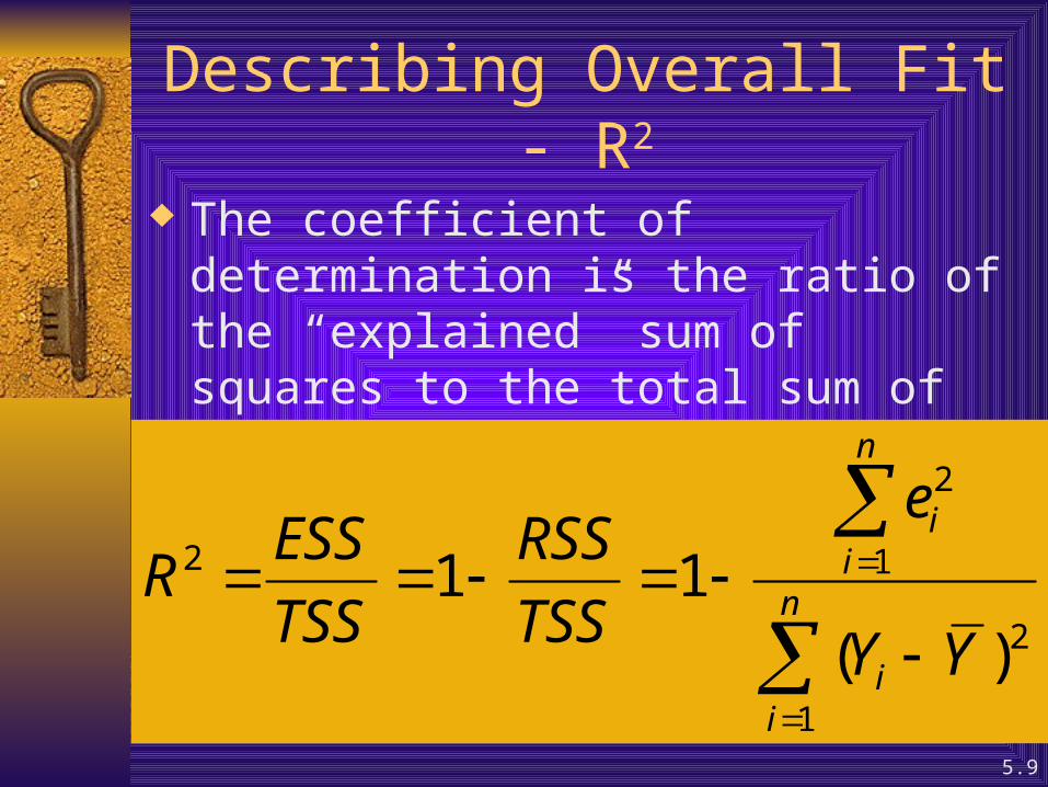
Describing Overall Fit - R2
The coefficient of determination is the ratio of the “explained” sum of squares to the total sum of squares
n
ii
n
ii
YY
e
TSSRSS
TSSESSR
1
2
1
2
2
)(11

5.10
Coefficient of Determination R2 yields the percentage of variability in Y
that is explained by the regression equation It ranges between 0 and 1 What is true if R2 = 1? What is true if R2 = 0?

5.11
Statistical Inference Drawing conclusions about the population
based on sample information. Hypothesis Testing
– which independent variables are significant?– Is the model significant?
Estimation - point versus interval– what is the rate of change in Y per X?– what is the expected value of Y based on X

5.12
Errors in Hypotheses Testing Type I error - rejecting the null hypothesis
when it is true Type II error - accepting the null hypothesis
when it is false Will never eliminate the possibility of error
- but can control their likelihood

5.13
Structuring the Null and Alternative Hypotheses
The null hypothesis is often the reverse of what theory or logic suggest the researcher believes; it is structured to allow the data to contradict it. In the model on the effect of price on quantity demanded, the researcher would expect price to inversely impact amount purchased. Thus, the null might be that price does not effect quantity demanded or it effects it in a positive direction.

5.14
Structuring the Null and Alternative Hypotheses
Model: QA=B0+B1PA+B2Inc+B3PB+
– QA = quantity demanded of good A
– PA = price of good A
– Inc = Income
– PB = price of good B
H0: B1 0
HA: B1 < 0 Law of Demand expectation

5.15
H0 : 1 = 0
Do Not Reject RejectReject
/2/2

5.16
H0 : 1 0
RejectDo Not Reject

5.17
H0 : 1 0
Do Not RejectReject

5.18
The t-Test for the Slope We can test the significance of an
independent variable by testing the following
H0 : k = 0 k = 1,2,….K
HA : k 0
Note if k = 0 a change in the kth independent variable has no impact on Y

5.19
The t-Test for the Slope The test statistic is
)ˆ(
ˆ0
k
Hkk SEt

5.20
T-Test Decision Rule The critical t-value, tc, is the value that
defines the boundary line separating the rejection from the do not reject region.
For a 2-tailed test if |tk| > tc, reject the null; otherwise do not reject
For a 1-tailed test if |tk| > tc and if tc has the sign implied by HA, reject the null; otherwise do not reject

5.21
F-Test and ANOVA F-Test is used to test the overall
significance of the regression or model Analysis of Variance = ANOVA ANOVA is based on the components of the
variation in Y previously discussed - TSS, ESS, and RSS

5.22
ANOVA Table
Source Sum of Sq df Mean Sq
Explain ESS K ESS/K
Residual RSS n-K-1 RSS/(n-K-1)
Total TSS n-1

5.23
F-Statistic
)1/(/
KnRSSKESSF
)1/()(
/)ˆ(2
2
KnYYKYY
Fi
i

5.24
Hypotheses for F-Test
H0: 1= 2=…..= K=0
HA: H0 is not true
Note the null suggests that all slopes are simultaneously zero and that the model would NOT be significant, ie. no independent variables are significant

5.25
Decision Rule for F-Test If F > Fc, reject the null that the model is
insignificant. Note this likely to be good news - your model appears “good”
Otherwise do not reject

5.26
Regression StatisticsMultiple R 0.954779929R Square 0.911604712Adjusted R Square 0.901205266Standard Error 13.29712264Observations 20
ANOVAdf SS MS F Significance F
Regression 2 30998.57408 15499.28704 87.65897183 1.10827E-09Residual 17 3005.829001 176.8134706Total 19 34004.40308
Coefficients Standard Error t Stat P-value Lower 95%Intercept -74.13868247 34.61202288 -2.141992183 0.046968174 -147.1637695N 11.32035941 0.952579754 11.88389671 1.16743E-09 9.310588995C 0.011554953 0.004032508 2.865451029 0.010718486 0.003047094
Illustration 5.3 page174-75

5.27
RESIDUAL OUTPUT
Observation Predicted P Residuals1 314.2437639 4.79623612 253.722741 1.2772589933 226.5899411 -1.0799411364 210.9690424 -2.0190424165 200.6312035 -0.4712034836 202.1897243 -5.9697243047 203.2398272 -11.439827198 188.8710569 2.5889430629 171.4279702 19.35202976
10 174.8906121 14.1193879111 190.1274017 -8.70740167212 178.1133956 1.62660438113 175.8412634 2.07873660214 151.8734723 24.7765277115 159.939179 11.44082116 182.8845429 -14.7745428617 149.7431674 11.2268326118 154.0752264 -3.05522640719 153.0044598 -23.1644598420 148.9420088 -22.60200882
San Mateo
Santa Barbara

5.28
Log_linear Model Constant percentage change in dependent
variable in response to a 1 percent change in an independent variable
no change in direction
cbZaXY

5.29
Double-Log Model Taking logs of the exponential equation
yields (note this is linear in the logs)
)(ln)(lnlnln ZcXbaY

5.30
Elasticity for Double Log Model The elasticity of Y with respect to X or Z
for a double- log model is merely the regression coefficient or b-hat or c-hat
Thus, in a double-log model the elasticities are constant and are merely equal to the estimated regression coefficients(partial slopes).