Basic Implementation of Multiple-Interval

Pseudospectral Methods to Solve Optimal

Control Problems

Technical Report UIUC-ESDL-2015-01

Daniel R. Herber∗

Engineering System Design LabUniversity of Illinois at Urbana-Champaign

June 4, 2015

Abstract

A short discussion of optimal control methods is presented including in-direct, direct shooting, and direct transcription methods. Next the basicsof multiple-interval pseudospectral methods are given independent of the nu-merical scheme to highlight the fundamentals. The two numerical schemesdiscussed are the Legendre pseudospectral method with LGL nodes and theChebyshev pseudospectral method with CGL nodes. A brief comparison be-tween time-marching direct transcription methods and pseudospectral directtranscription is presented. The canonical Bryson-Denham state-constraineddouble integrator optimal control problem is used as a test optimal controlproblem. The results from the case study demonstrate the effect of user’schoice in mesh parameters and little difference between the two numericalpseudospectral schemes.

∗Ph.D pre-candidate in Systems and Entrepreneurial Engineering, Department of In-dustrial and Enterprise Systems Engineering, University of Illinois at Urbana-Champaign,herber1@illinois.educ©2015 Daniel R. Herber

1

Contents

1 Optimal Control and Direct Transcription 3

2 Basics of Pseudospectral Methods 42.1 Foundation . . . . . . . . . . . . . . . . . . . . . . . . . . . . . . . . 42.2 Multiple Intervals . . . . . . . . . . . . . . . . . . . . . . . . . . . . 72.3 Legendre Pseudospectral Method with LGL Nodes . . . . . . . . . . 92.4 Chebyshev Pseudospectral Method with CGL Nodes . . . . . . . . . 102.5 Brief Comparison to Time-Marching Direct Transcription Methods 11

3 Numeric Case Study 143.1 Test Problem Description . . . . . . . . . . . . . . . . . . . . . . . . 143.2 Implementation and Analysis Details . . . . . . . . . . . . . . . . . . 143.3 Summary of Case Study Results . . . . . . . . . . . . . . . . . . . . 15

A Case Studies 19A.1 Select Command Window Outputs . . . . . . . . . . . . . . . . . . . 19A.2 Select Solution and Error Plots . . . . . . . . . . . . . . . . . . . . . 20

B Visualizations for Specific Pseudospectral Implementations 24

C Supplementary MATLABr Code 28

List of Figures

1 Illustration of a state variable in multiple-interval PS methods . . . 72 Solution and error plots for tests {1, 3, 5} with LGL nodes . . . . . . 213 Solution and error plots for tests {7, 11, 13} with LGL nodes . . . . . 224 Solution and error plots for tests {7, 11, 13} with CGL nodes . . . . 235 LGL and CGL inner node locations from the roots of polynomials . 246 ED, CGL, and LGL nodes for various values of Nt . . . . . . . . . . 257 Lagrange polynomial interpolation with ED, LGL, and CGL nodes . 258 Differentiation error using Lagrange interpolation with LGL nodes . 269 Convergence behavior for definite integral and derivative approxima-

tions using Lagrange interpolation with LGL nodes . . . . . . . . . . 2710 Algorithm flowchart of supplementary MATLAB code . . . . . . . . 28

List of Tables

1 Results for different meshes using LGL nodes . . . . . . . . . . . . . 162 Results for different meshes using CGL nodes . . . . . . . . . . . . . 16

2

1 Optimal Control and Direct Transcription

Consider the following general optimal control problem:

minu(t),t0,tf

∫ tf

t0

L (t, ξ(t),u(t)) dt+M (t0, ξ(t0), tf , ξ(tf )) (1a)

subject to: ξ − fd (t, ξ(t),u(t)) = 0 (1b)

C (t, ξ(t),u(t)) ≤ 0 (1c)

φ (t0, ξ(t0), tf , ξ(tf )) ≤ 0 (1d)

where t, ξ(t), and u(t) are the time, state, and control trajectories defined on thetime horizon t ∈ [t0, tf ]. Problem (1) then consists of the Lagrange term L(·) andMayer termM(·) in Eqn. (1a), the dynamic constraints in Eqn. (1b), the algebraicpath constraints C(·) in Eqn. (1c), and the boundary constraints φ(·) in Eqn. (1d).Time-invariant optimization variables (e.g., plant variables in co-design [Her14a])may be included as well but are beyond the scope of this report.

Note that Prob. (1) contains u(t) as an optimization variable. This quantity isinfinite-dimensional since it needs to be defined for for all values in t ∈ [t0, tf ].Indirect methods of optimal control such as Pontryagin’s maximum principle werethe initial solution techniques [Lib12, p. 102]. There are a number of issues withusing indirect methods (either analytically or numerically), so direct methods areoften employed [Her14a, pp. 25–26].

Direct methods of optimal control are known as discretize-then-optimize (D → O)methods [Bie07, pp. 243–246]. These methods do not use calculus of variationsor directly state the optimality conditions. Instead, the control and/or state areparametrized using function approximation and the cost is approximated using nu-merical quadrature [Rao12, p. 141]. This creates a discrete, finite-dimensional prob-lem that can then solved using large-scale NLP solvers [Bie07, pp. 243–246]. Thisformulation requires an accurate level of parameterization of the control (and possi-bly the state) profiles. There are two main classes of direct methods: sequential andsimultaneous. Sequential methods only parametrize the control while simultaneousmethods parametrize both the state and control. In both methods, the parametersthat define the parameterization are included as optimization variables. Sequentialmethods include both shooting and multiple shooting formulations which utilizea nested differential-algebraic equation solver (simulation) to satisfy the dynamicconstraints. The simultaneous approach on the other hand simultaneously searchesfor the optimal solution and feasible dynamic constraints. Sequential approachestypically produce low-quality solutions and are computationally inefficient, i.e., com-pared to simultaneous methods [Her14a, pp. 26–28].

The simultaneous or direct transcription (DT) problem formulation is:

minΞ,U,t0,tf

Nt∑k=0

wkL (tk, ξ(tk),u(tk)) +M (t0, ξ(t0), tf , ξ(tf )) (2a)

subject to: ζ (t,Ξ,U) = 0 (2b)

C (t,Ξ,U) ≤ 0 (2c)

φ (t0, ξ(t0), tf , ξ(tf )) ≤ 0 (2d)

3

whereNt+1 is the number of discrete time points and t, Ξ, and U are the discretizedforms of the time, states, and controls. The Lagrange term is approximated withnumerical quadrature with weights wk. The dynamic constraint is now enforcedthrough a large number of equality constraints ζ(·), termed defect constraints. DTapproaches can either have either local or global support termed time-marchingmethods or pseudospectral methods, respectively [Her14a, p. 29]. The primaryfocus of this technical report is pseudospectral methods.

2 Basics of Pseudospectral Methods

Here we discuss how to approximate the infinite-dimensional Prob. (1) as the finite-dimensional Prob. (2) with pseudospectral (PS) methods, one class of direct tran-scription methods. PS methods parametrize both the control and state using func-tion approximation and the cost using numerical quadrature [Rao12, p. 141]. Somegeneral references on various types of PS methods include Refs. [FR02, FR08,BGa10, Rao12]. A number of software packages exist to implement PS methodsincluding GPOPS− II [PR14], PSOPT [Bec11], and PROPT [RE10].

Section 2.1 provides the foundational elements for PS methods independent of par-ticular choice of nodes, basis function, etc. for a single polynomial defined over thetime horizon. Next in Sec. 2.2 we extend the PS approach to multiple-intervals eachcontaining a distinct polynomial approximation. In Secs. 2.3 and 2.4 we outline thenodes, basis function, etc. for two particular numerical schemes. Finally, Sec. 2.5briefly compares PS methods to the time-marching DT methods.

2.1 Foundation

2.1.1 Transformation to τ

We define a new independent, scaled time variable τ instead of t as:

τ =2

tNt − t0t− tNt + t0

tNt − t0(3)

where τ ∈ [−1, 1] for any value of t0 and tNt ≡ tf .

2.1.2 Interpolation with Polynomials

Given a set of node points τ = [τ0, τ1, . . . , τNt ]T containing Nt+1 increasing distinct

numbers in [−1, 1] and f(τ) is a function whose values are given at τ , then a uniquepolynomial P (τ) of degree at most Nt exists with:

f(τk) = P (τk), k = {0, 1, . . . , Nt} (4)

The interpolating polynomial of f(τ) is defined as:

f(τ) ≈ P (τ) =

Nt∑k=0

f(τk)φk(τ) (5)

where φk(·) are continuous basis polynomials that are typically constructed suchthat the property in Eqn. (4) holds, i.e., interpolating f(τ) at the node points.Therefore, the polynomial approximation is exact at the node points and an ap-proximation at all other values of τ .

4

2.1.3 Approximate Differentiation

The derivative (d/dτ) of f(τ) can be approximated with dP (τ)/dτ :

f(τk) ≈ P (τk) =

Nt∑i=0

Dkif(τi) (6)

where the (Nt + 1)× (Nt + 1) matrix D is termed the differentiation matrix. Thismatrix depends only on the values of τ and the type of interpolating polynomial,so we have an approximation for the f(τ ) that depends only on f(τ ).

2.1.4 Numerical Quadrature

We first note that the transformation in Eqn. (3) scales the integral term:∫ tNt

t0

f(t)dt =tNt − t0

2

∫ 1

−1

f(τ)dτ (7)

For a function f(τ), the integral over τ ∈ [−1, 1] can be approximated with aquadrature scheme: ∫ 1

−1

f(τ) ≈Nt∑k=0

wkf(τk) (8)

where wk are predetermined quadrature weights. These weights depend only on thevalues of τ and the type of interpolating polynomial, so we have an approximationof the definite integral that is a sum of predefined weighted values of f(τ ).

2.1.5 Discretization Matrices and Optimization Variable Vector

For simplicity, we denote the derivative function and the time step of the entiretime horizon as:

fd(τ) fd (τ, ξ(τ),u(τ)) (9)

h = tNt − t0 (10)

We define the following matrices that contain the discreztized components of Prob. (1):

Ξ =

ξ(τ0)...

ξ(τNt)

=

ξ1(τ0) · · · ξnξ(τ0)...

. . ....

ξ1(τNt) · · · ξnξ(τNt)

(Nt+1)×nξ

(11a)

U =

u(τ0)...

u(τNt)

=

u1(τ0) · · · unu(τ0)...

. . ....

u1(τNt) · · · unu(τNt)

(Nt+1)×nu

(11b)

F =h

2

fd(τ0)...

fd(τNt)

=h

2

fd1(τ0) · · · fdnξ(τ0)...

. . ....

fd1(τNt) · · · fdnξ(τNt)

(Nt+1)×nξ

(11c)

5

C =

C(τ0)...

C(τNt)

=

C1(τ0) · · · CnC (τ0)...

. . ....

C1(τNt) · · · CnC (τNt)

(Nt+1)×nC

(11d)

φ =[φ1 · · · φnφ

]1×nφ

(11e)

where nξ, nu, nC , and nφ are the number of states, controls, path constraints, andboundary constraints, respectively. We briefly note here that C ≤ 0 and φ ≤ 0 nowcan be included directly in the NLP formulation although constraint satisfactionof C is only at the finite set of node points. In addition, the optimization variablevector dimension scales linearly with Nt:

x =

vec(Ξ)vec(U)t0tf

(Nt+1)×(nξ+nu)+2

(12)

where the function vec(·) reorganizes the matrix input to a single column vectorcontaining all entries of the input matrix.

2.1.6 Defect Constraints

To represent accurately the dynamics in Prob. (1b), we need to ensure that ourapproximation for the state derivatives using Eqn. (6) is equivalent to the derivativefunction values given by fd(τ). This enforced with equality constraints in matrixform:

ζ = 0

= DΞ− F (13)

recalling that D is the differentiation matrix defined in Eqn. (6), Ξ is the matrixof discretized state values defined in Eqn. (11a), and F is the matrix of derivativefunction values defined in Eqn. (11c).

2.1.7 Objective Function

The definite integral with the Lagrange term in Eqn. (2a) can be approximated by:

Nt∑k=0

wkL (tk, ξ(tk),u(tk)) =h

2

Nt∑k=0

wkL (τk, ξ(τk),u(τk)) (14)

For simplicity, we denote the Lagrange term as:

L (τk) L (τk, ξ(τk),u(τk)) (15)

The Mayer term is simply:

M (t0, ξ(t0), tNt , ξ(tNt)) =M (t0, ξ(−1), tNt , ξ(1)) (16)

6

⇠(t)

tt0 = t(0) t(3) = tf

⇠(1)(⌧4)� ⇠(2)(⌧0)

⇠(2)(⌧3)� ⇠(3)(⌧0)�1

�2} }

} }}C1(⌧(2)2 )

}C1(⌧(3)0 )

t(1) t(2)

C1(t)

I(1) : N(1)t = 4

⌧(1)4 = 1

⌧(1)3

⌧(1)2

⌧(1)1

⌧(1)0 = �1

P (1)

I(2) : N(2)t = 3

P (2)

⌧(3)4 = �1

⌧(3)3

⌧(3)2

⌧(3)1

⌧(3)0 = 1

P (3)

I(3) : N(3)t = 4

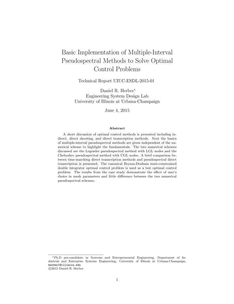
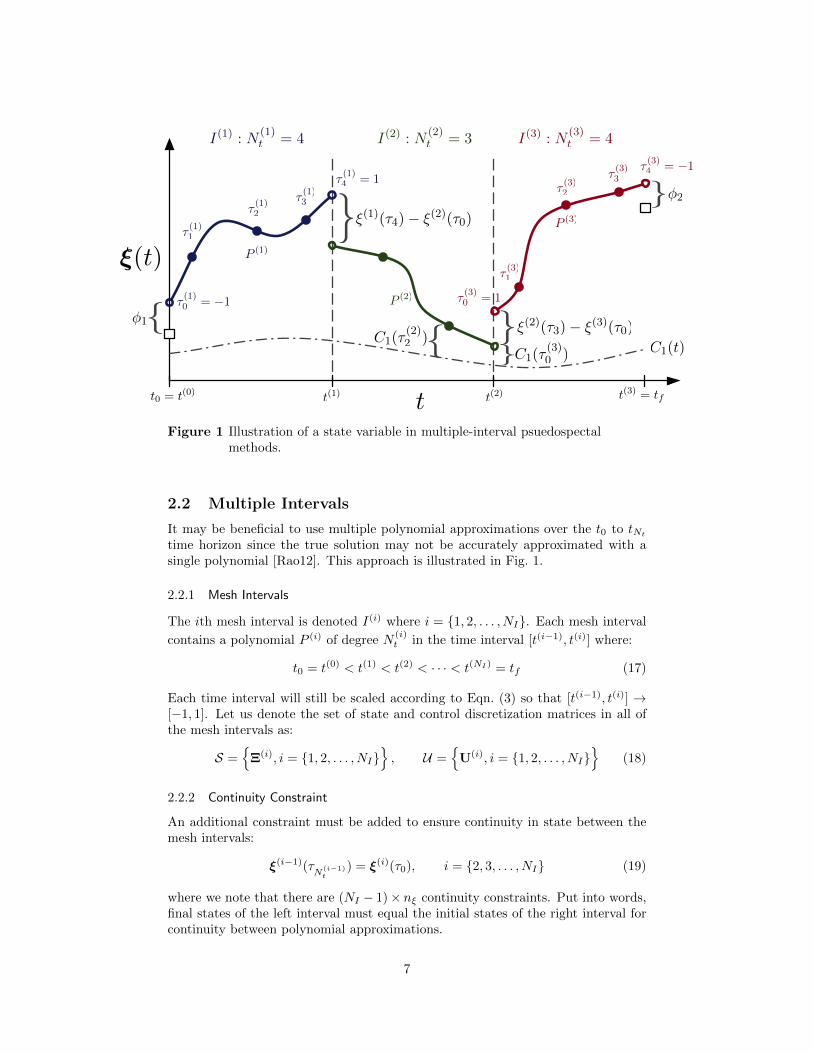
Figure 1 Illustration of a state variable in multiple-interval psuedospectalmethods.

2.2 Multiple Intervals

It may be beneficial to use multiple polynomial approximations over the t0 to tNttime horizon since the true solution may not be accurately approximated with asingle polynomial [Rao12]. This approach is illustrated in Fig. 1.

2.2.1 Mesh Intervals

The ith mesh interval is denoted I(i) where i = {1, 2, . . . , NI}. Each mesh interval

contains a polynomial P (i) of degree N(i)t in the time interval [t(i−1), t(i)] where:

t0 = t(0) < t(1) < t(2) < · · · < t(NI) = tf (17)

Each time interval will still be scaled according to Eqn. (3) so that [t(i−1), t(i)] →[−1, 1]. Let us denote the set of state and control discretization matrices in all ofthe mesh intervals as:

S ={

Ξ(i), i = {1, 2, . . . , NI}}, U =

{U(i), i = {1, 2, . . . , NI}

}(18)

2.2.2 Continuity Constraint

An additional constraint must be added to ensure continuity in state between themesh intervals:

ξ(i−1)(τN

(i−1)t

) = ξ(i)(τ0), i = {2, 3, . . . , NI} (19)

where we note that there are (NI − 1)× nξ continuity constraints. Put into words,final states of the left interval must equal the initial states of the right interval forcontinuity between polynomial approximations.

7

2.2.3 Multiple-Interval Formulation

The complete multiple-interval formulation of Prob. (2) is:

minS,U,t0,tf

NI∑i=1

h(i)

2

N(i)t∑

k=0

w(i)k L

(τ

(i)k

)+M(t0, ξ

(1)(−1), tf , ξ(NI)(1)

)(20a)

subject to: ζ(τ (i),Ξ(i),U(i)

)= 0 i = {1, 2, . . . , NI} (20b)

C(τ (i),Ξ(i),U(i)

)≤ 0 i = {1, 2, . . . , NI} (20c)

φ(t0, ξ

(1)(−1), tf , ξ(NI)(1)

)≤ 0 (20d)

ξ(i−1)(τN

(i−1)t

)− ξ(i)(τ0) = 0 i = {2, 3, . . . , NI} (20e)

The problem size now additionally depends on the number of intervals NI and their

respective number of nodes points N(i)t .

8

2.3 Legendre Pseudospectral Method with LGL Nodes

This section outlines one particular numerical scheme for finding the nodes, differ-entiation matrix, and quadrature weights for use in pseudospectral methods.

2.3.1 Nodes

Let LN (τ) denote the Legendre polynomial of order N , which may be generatedfrom:

LN (τ) =1

2NN !

dN

dτN(τ2 − 1

)N(21)

The Lagrange-Gauss-Lobatto (LGL) nodes are defined as:

τk =

−1 if k = 0

kth root of LNt(τ) if k = {1, 2, . . . , Nt − 1}1 if k = Nt

(22)

where LN = dLNdτ . We note that the nodes are always between [−1, 1] and contain

both endpoints (App. C code from Ref. [STW11]).

2.3.2 Interpolating Polynomial Basis Function

We define the basis polynomials needed in Eqn. (5) for the Legendre-based methodas Lagrange basis polynomials:

φk(τ) =

Nt∏i=0,i6=k

τ − τiτk − τi

(23)

With LGL nodes, φk(τ) can be written in the following alternative form [BGa10]:

φk(τ) =1

Nt (Nt + 1)LNt(τk)

(τ2 − 1)LNt(τ)

τ − τk(24)

2.3.3 Approximate Differentiation

The differentiation matrix needed in Eqn. (6) for the Legendre-based method is:

Dki =

LNt (τk)

LNt (τi)1

τk−τi if k 6= i

Nt(Nt + 1)/4 if k = i = 0

−Nt(Nt + 1)/4 if k = i = Nt

0 otherwise

(25)

Further numerical enhancements can be made to improve stability in the presenceof rounding errors (expression from Ref. [BGa10], App. C code from Ref. [STW11]).

2.3.4 Quadrature Weights

The quadrature weights wk needed in Eqn. (8) for the Legendre-based method are:

wk =2

Nt(Nt + 1)

1

(LNt(τk))2 , k = {0, 1, . . . , Nt} (26)

These are Gaussian quadrature weights that are exactly accurate for polynomialsof degree up to degree 2Nt − 1 (expression from Ref. [FR08], App. C code fromRef. [STW11]).

9

2.4 Chebyshev Pseudospectral Method with CGL Nodes

This section outlines one particular numerical scheme for finding the nodes, differ-entiation matrix, and quadrature weights for use in pseudospectral methods.

2.4.1 Nodes

Let TN (τ) denote the Chebyshev polynomial of order N , which may be generatedfrom:

TN = cos(N cos−1 (τ)

)(27)

The Chebyshev-Gauss-Lobatto (CGL) nodes are defined as the roots of TNt =dTNtdτ

and the additional endpoints. All CGL nodes can be computed conveniently by:

τk = − cos

(πk

Nt

)k = {0, 1, . . . , Nt} (28)

We note that the nodes are always between [−1, 1] and contain both endpoints.

2.4.2 Interpolating Polynomial Basis Function

We define the basis polynomials needed in Eqn. (5) for the Chebyshev-based methodas Lagrange basis polynomials previously defined in Eqn. (23). With CGL nodes,φk(τ) can be written in the following alternative form [FR02]:

φk(τ) =(−1)k+1

N2t ak

(1− τ2)TNt(τ)

τ − τkwhere: ak =

{2 if k = {0, Nt}1 otherwise

(29)

2.4.3 Approximate Differentiation

The differentiation matrix needed in Eqn. (6) for the Chebyshev-based method is:

Dki =

akai

(−1)k+i

(τk−τi) if k 6= i

− τk2(1−τ2

k)if 1 ≤ k = i ≤ Nt − 1

2N2t +16 if k = i = 0

− 2N2t +16 if k = i = Nt

(30)

Further numerical enhancements can be made to improve stability in the presenceof rounding errors (expression from Ref. [FR02], App. C code from [Tre00, p. 54]).

2.4.4 Quadrature Weights

The quadrature weights wk needed in Eqn. (8) for the Chebyshev-based methodare:

wk =ckNt

1−bNt/2c∑j=1

bj4j2 − 1

cos (2jτk)

(31)

where: bj =

{1 if j = Nt/2

2 if j < Nt/2, ck =

{1 if k = {0, Nt}2 otherwise

These are Clenshaw-Curtis quadrature weights that are exactly accurate for poly-nomials of degree up to degree Nt (expression from Ref. [Wal06], App. C code fromRef. [Tre00, p. 128]).

10

2.5 Brief Comparison to Time-Marching Direct Transcrip-tion Methods

2.5.1 Foundation

Time-marching DT methods approach the satisfaction of the differential equationin Eqn. (2b) in a slightly different manner than PS methods although both canproduce approximately feasible dynamics when the defect constraints are satisfied.

Consider the following integral equation that provides a solution to ξ = fd (·) for agiven initial condition over the t ∈ [t0, tf ] time horizon:

ξ(tf ) = ξ(t0) +

∫ tf

t0

fd (s, ξ(s),u(s)) ds (32)

A common approach for approximating this type of equation is the class of Runge-Kutta methods which only directly require the knowledge of the state and controlvalues at the interval boundaries [Bet10, pp. 97–100]. However, these methods areonly accurate with a sufficiently small step sizes. Therefore we will take the sameapproach as Sec. 2.2: multiple-intervals.

Reconsider Eqn. (17) which defined the temporal relationship between the time

interval boundaries. If we take N(i)t = 1 ∀i ∈ {1, 2, . . . , NI}, then each interval

would only contain the scaled points −1 and 1. Based this structure, we will forgothe continuity equation in Eqn. (19) and instead use a single value for the final pointof the I(i−1) and initial point of I(i). Therefore we will have a Nt = NI relationshipand NI + 1 time points so we can write t(i) ti for convenience. We now considerthe mesh interval I(i) in the time interval [ti−1, ti], then we seek a solution to thefollowing integral equation:

ξ(ti) = ξ(ti−1) +

∫ ti

ti−1

fd (s, ξ(s),u(s)) ds (33)

Now we can rewrite Eqn. (33) to determine the defect constraints:

ζ(ti) ζ (ti−1, ti, ξ(ti−1), ξ(ti),u(ti−1),u(ti)) (34a)

ζ(ti) = 0, i = {1, 2, . . . , Nt} (34b)

ζ(ti) = ξ(ti)− ξ(ti−1)−∫ ti

ti−1

fd (s, ξ(s),u(s)) ds (34c)

We will now consider two simple Runge-Kutta schemes. For a more complete list ofschemes and a more through treatment of time-marching DT methods please referto Refs. [Bet10, Bie10, Her14a].

2.5.2 Euler Forward and Trapezoidal Defect Constraints

The Euler forward method is an explicit first-order scheme:

ζ(ti) = ξ(ti)− ξ(ti−1)− hifd(ti−1) (35)

The trapezoidal rule is an implicit second-order scheme:

ζ(ti) = ξ(ti)− ξ(ti−1)− hi2

(fd(ti) + fd(ti−1)) (36)

11

2.5.3 Lagrange Term Quadrature

Consider the following transformation (see Ref. [Lib12, p. 87] for the assumptionsrequired on L): ∫ tf

t0

L(t, ξ,u)dt = ξ0(tf ) (37a)

ξ0 = L(t, ξ,u), ξ0(t0) = 0 (37b)

This transformation adds an additional state variable ξ0 with the dynamics nat-urally equivalent to L with an arbitrary initial value for the ordinary differentialequation (ODE). The final value ξ0(tf ) can then be included in the Mayer term.For simplicity we denote the Lagrange term as:

L(ti) L(ti, ξ(ti),u(ti)) (38)

Now if we apply the Euler forward method to the ODE in Eqn. (37b), we arrive atthe following composite quadrature method:∫ tf

t0

L (t) dt ≈Nt−1∑i=0

hiL (ti) (39)

This is a composite quadrature method since we are using a set of points inside thetime horizon to better approximate the definite integral [Hea02, p. 255]. Similarly ifwe apply the trapezoidal rule to the ODE in Eqn. (37b), we arrive at the followingcomposite quadrature method:∫ tf

t0

L (t) dt ≈ 1

2

Nt∑i=0

hi (L (ti) + L (ti−1)) (40)

2.5.4 Remaining Problem Formulation Elements

The path and boundary constraint matrices in Eqns. (11d) and (11e) can be in-cluded in the NLP formulation in the same manner as they were for the PS methodapproach. As previously mentioned, there will be no continuity constraints. Withthe defect constraint and quadrature approaches are outlined, all the necessary nu-merical concepts to solve Prob. (2) with a time-marching DT method have beendescribed.

2.5.5 Comparison

Here are a couple of comparison points between pseudospectral methods and time-marching approaches.

• At a superficial level, PS methods satisfy the dynamics by ensuring the deriva-tives of the approximation are sufficiently accurate while time-marching meth-ods accomplish this task through a sufficiently accurate step size betweensuccessive state values in the ODE approximation scheme.

• The two DT approaches are called a number of terms in the literature. Thesevarious names are summarized in the following table:

12

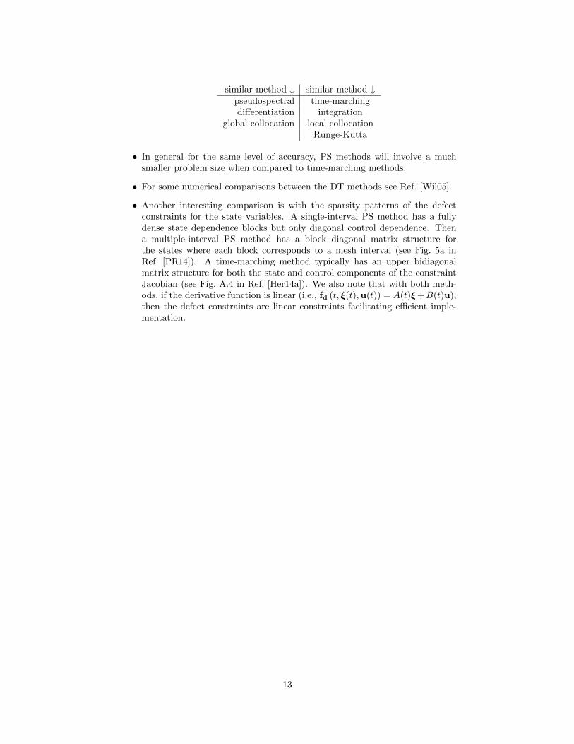
similar method ↓ similar method ↓pseudospectral time-marchingdifferentiation integration

global collocation local collocationRunge-Kutta

• In general for the same level of accuracy, PS methods will involve a muchsmaller problem size when compared to time-marching methods.

• For some numerical comparisons between the DT methods see Ref. [Wil05].

• Another interesting comparison is with the sparsity patterns of the defectconstraints for the state variables. A single-interval PS method has a fullydense state dependence blocks but only diagonal control dependence. Thena multiple-interval PS method has a block diagonal matrix structure forthe states where each block corresponds to a mesh interval (see Fig. 5a inRef. [PR14]). A time-marching method typically has an upper bidiagonalmatrix structure for both the state and control components of the constraintJacobian (see Fig. A.4 in Ref. [Her14a]). We also note that with both meth-ods, if the derivative function is linear (i.e., fd (t, ξ(t),u(t)) = A(t)ξ+B(t)u),then the defect constraints are linear constraints facilitating efficient imple-mentation.

13

3 Numeric Case Study

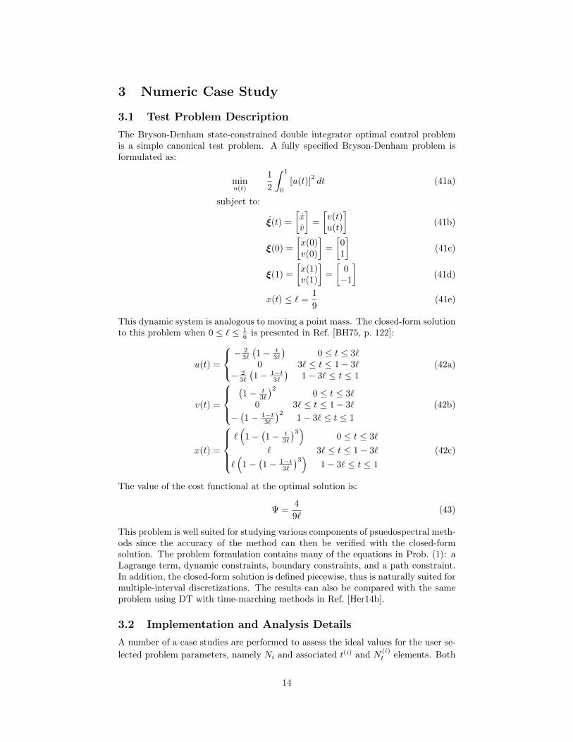
3.1 Test Problem Description

The Bryson-Denham state-constrained double integrator optimal control problemis a simple canonical test problem. A fully specified Bryson-Denham problem isformulated as:

minu(t)

1

2

∫ 1

0

[u(t)]2dt (41a)

subject to:

ξ(t) =

[xv

]=

[v(t)u(t)

](41b)

ξ(0) =

[x(0)v(0)

]=

[01

](41c)

ξ(1) =

[x(1)v(1)

]=

[0−1

](41d)

x(t) ≤ ` =1

9(41e)

This dynamic system is analogous to moving a point mass. The closed-form solutionto this problem when 0 ≤ ` ≤ 1

6 is presented in Ref. [BH75, p. 122]:

u(t) =

−23`

(1− t

3`

)0 ≤ t ≤ 3`

0 3` ≤ t ≤ 1− 3`− 2

3`

(1− 1−t

3`

)1− 3` ≤ t ≤ 1

(42a)

v(t) =

(1− t

3`

)20 ≤ t ≤ 3`

0 3` ≤ t ≤ 1− 3`

−(1− 1−t

3`

)21− 3` ≤ t ≤ 1

(42b)

x(t) =

`(

1−(1− t

3`

)3)0 ≤ t ≤ 3`

` 3` ≤ t ≤ 1− 3`

`(

1−(1− 1−t

3`

)3)1− 3` ≤ t ≤ 1

(42c)

The value of the cost functional at the optimal solution is:

Ψ =4

9`(43)

This problem is well suited for studying various components of psuedospectral meth-ods since the accuracy of the method can then be verified with the closed-formsolution. The problem formulation contains many of the equations in Prob. (1): aLagrange term, dynamic constraints, boundary constraints, and a path constraint.In addition, the closed-form solution is defined piecewise, thus is naturally suited formultiple-interval discretizations. The results can also be compared with the sameproblem using DT with time-marching methods in Ref. [Her14b].

3.2 Implementation and Analysis Details

A number of a case studies are performed to assess the ideal values for the user se-

lected problem parameters, namely Ni and associated t(i) and N(i)t elements. Both

14

the Legendre PS method with LGL nodes and Chebyshev PS method with CGLnodes are used.

Algorithm/TolerancesEach problem is solved using the fmincon solver using the sqp algorithm. The defaulttolerances were used:

TolCon = 1e-6; TolFun = 1e-6; TolX = 1e-6; TolConSQP = 1e-6;

Performance MetricsAbsolute error e will be calculated with respect to the closed-form solution inEqn. (42) and closed-form objective function value in Eqn. (43):

absolute error = |actual− approx| (44)

The accuracy of a trajectory will be assessed with the maximum absolute error onthe interval. A final metric will be the total CPU time1 to assess the expectedtrade-offs between accuracy and computation time.

Initial GuessInitial guesses are important when using direct methods of optimal control [Wil05].Here a linear initial trajectory between the state boundary conditions was used andan all zero initial control guess.

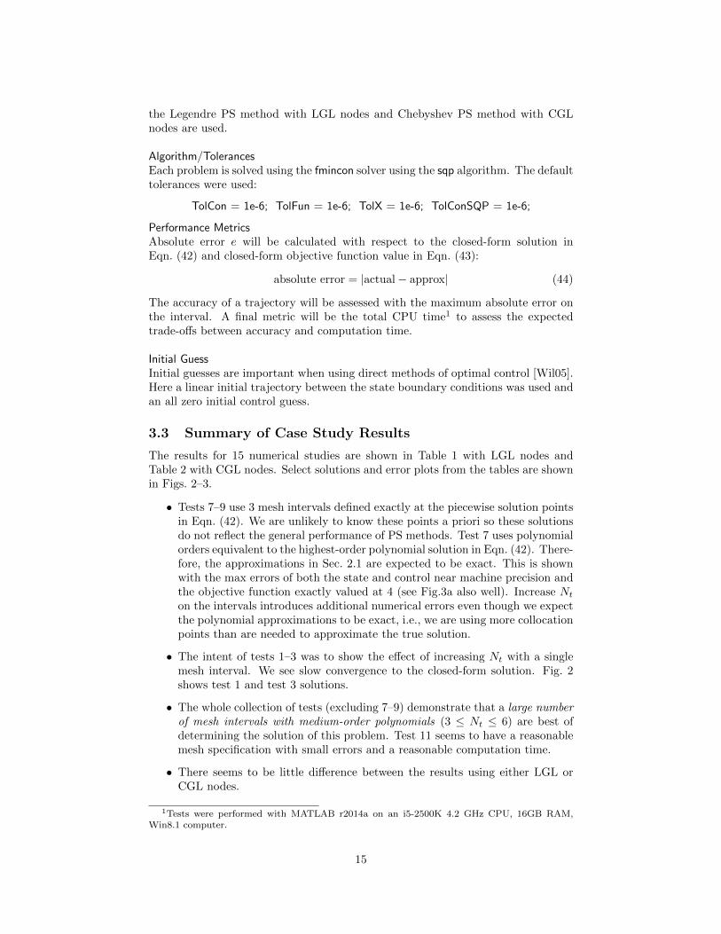
3.3 Summary of Case Study Results

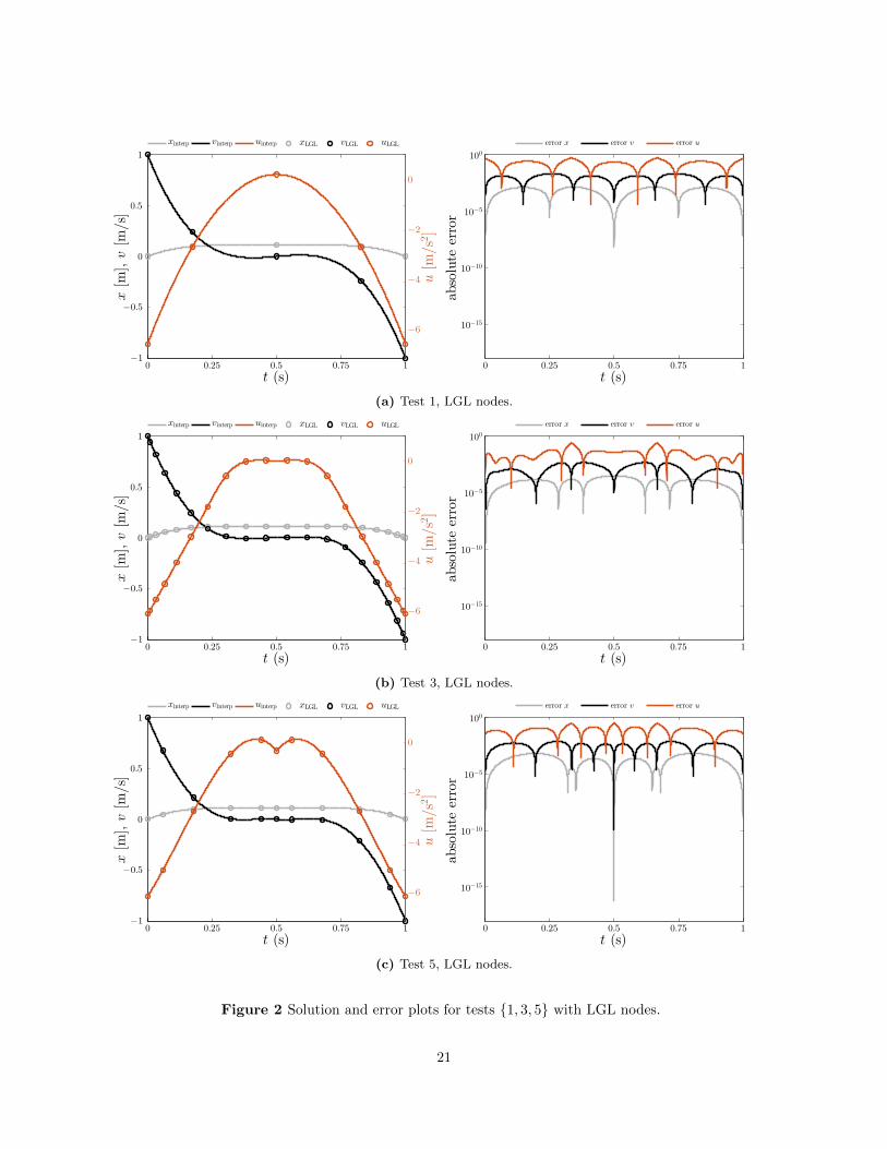
The results for 15 numerical studies are shown in Table 1 with LGL nodes andTable 2 with CGL nodes. Select solutions and error plots from the tables are shownin Figs. 2–3.

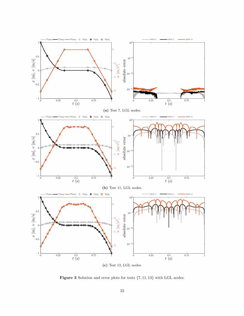
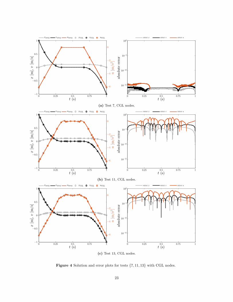
• Tests 7–9 use 3 mesh intervals defined exactly at the piecewise solution pointsin Eqn. (42). We are unlikely to know these points a priori so these solutionsdo not reflect the general performance of PS methods. Test 7 uses polynomialorders equivalent to the highest-order polynomial solution in Eqn. (42). There-fore, the approximations in Sec. 2.1 are expected to be exact. This is shownwith the max errors of both the state and control near machine precision andthe objective function exactly valued at 4 (see Fig.3a also well). Increase Nton the intervals introduces additional numerical errors even though we expectthe polynomial approximations to be exact, i.e., we are using more collocationpoints than are needed to approximate the true solution.

• The intent of tests 1–3 was to show the effect of increasing Nt with a singlemesh interval. We see slow convergence to the closed-form solution. Fig. 2shows test 1 and test 3 solutions.

• The whole collection of tests (excluding 7–9) demonstrate that a large numberof mesh intervals with medium-order polynomials (3 ≤ Nt ≤ 6) are best ofdetermining the solution of this problem. Test 11 seems to have a reasonablemesh specification with small errors and a reasonable computation time.

• There seems to be little difference between the results using either LGL orCGL nodes.

1Tests were performed with MATLAB r2014a on an i5-2500K 4.2 GHz CPU, 16GB RAM,Win8.1 computer.

15

Table 1 Results for different meshes using LGL nodes.

Test t N(i)t eΨ max ex max ev max eu tCPU (s)

1 [0, 1] 4 2× 10−2 1× 10−3 2× 10−2 5× 10−1 0.05

2 [0, 1] 9 4× 10−2 2× 10−3 2× 10−2 5× 10−1 0.17

3 [0, 1] 19 4× 10−3 3× 10−4 5× 10−3 2× 10−1 2.99

4 [0, 12 , 1] 3 8× 10−2 8× 10−3 8× 10−2 2× 100 0.11

5 [0, 12 , 1] 5 5× 10−3 7× 10−4 8× 10−3 3× 10−1 0.53

6 [0, 12 , 1] 9 6× 10−3 5× 10−4 8× 10−3 3× 10−1 2.82

7 [0, 3`, 1− 3`, 1] [3, 1, 3] 1× 10−15 1× 10−16 4× 10−16 4× 10−15 0.16

8 [0, 3`, 1− 3`, 1] [5, 1, 5] 5× 10−10 2× 10−9 2× 10−8 1× 10−6 0.37

9 [0, 3`, 1− 3`, 1] 5 4× 10−12 3× 10−8 3× 10−7 1× 10−5 2.40

10 linspace(0, 1, 6) 3 2× 10−2 3× 10−3 3× 10−2 6× 10−1 0.87

11 linspace(0, 1, 6) 5 4× 10−4 1× 10−4 2× 10−3 2× 10−1 7.35

12 linspace(0, 1, 6) 9 4× 10−4 1× 10−4 1× 10−3 1× 10−1 40.35

13 linspace(0, 1, 11) 3 2× 10−3 2× 10−4 6× 10−3 3× 10−1 8.81

14 linspace(0, 1, 11) 5 3× 10−5 2× 10−4 2× 10−3 8× 10−2 51.60

15 linspace(0, 1, 11) 9 4× 10−5 3× 10−5 3× 10−4 6× 10−2 269.39

Table 2 Results for different meshes using CGL nodes.

Test t N(i)t eΨ max ex max ev max eu tCPU (s)

1 [0, 1] 4 2× 10−2 1× 10−3 2× 10−2 5× 10−1 0.05

2 [0, 1] 9 5× 10−2 2× 10−3 3× 10−2 5× 10−1 0.17

3 [0, 1] 19 5× 10−3 4× 10−4 6× 10−3 3× 10−1 3.14

4 [0, 12 , 1] 3 5× 10−2 7× 10−3 8× 10−2 2× 100 0.11

5 [0, 12 , 1] 5 5× 10−3 5× 10−4 6× 10−3 4× 10−1 0.68

6 [0, 12 , 1] 9 6× 10−3 5× 10−4 7× 10−3 3× 10−1 2.87

7 [0, 3`, 1− 3`, 1] [3, 1, 3] 4× 10−15 1× 10−16 8× 10−16 7× 10−15 0.17

8 [0, 3`, 1− 3`, 1] [5, 1, 5] 7× 10−15 2× 10−9 1× 10−8 5× 10−7 0.46

9 [0, 3`, 1− 3`, 1] 5 2× 10−12 2× 10−8 2× 10−7 6× 10−6 2.41

10 linspace(0, 1, 6) 3 1× 10−2 3× 10−3 3× 10−2 6× 10−1 0.88

11 linspace(0, 1, 6) 5 4× 10−4 7× 10−5 2× 10−3 1× 10−1 7.76

12 linspace(0, 1, 6) 9 4× 10−4 1× 10−4 1× 10−3 1× 10−1 40.59

13 linspace(0, 1, 11) 3 1× 10−3 2× 10−4 6× 10−3 3× 10−1 8.88

14 linspace(0, 1, 11) 5 3× 10−5 1× 10−4 1× 10−3 7× 10−2 56.79

15 linspace(0, 1, 11) 9 6× 10−5 3× 10−5 4× 10−4 6× 10−2 258.26

16

Acknowledgments

I would like to thank Assistant Professor James Allison2 at the University of Illinoisat Urbana-Champaign who provided much assistance when preparing this report.

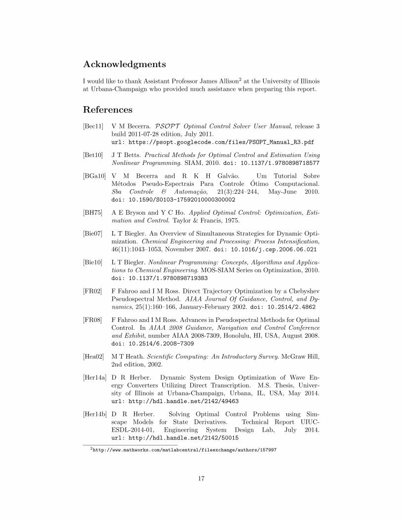
References

[Bec11] V M Becerra. PSOPT Optimal Control Solver User Manual, release 3build 2011-07-28 edition, July 2011.url: https://psopt.googlecode.com/files/PSOPT_Manual_R3.pdf

[Bet10] J T Betts. Practical Methods for Optimal Control and Estimation UsingNonlinear Programming. SIAM, 2010. doi: 10.1137/1.9780898718577

[BGa10] V M Becerra and R K H Galvao. Um Tutorial SobreMetodos Pseudo-Espectrais Para Controle Otimo Computacional.Sba Controle & Automacao, 21(3):224–244, May-June 2010.doi: 10.1590/S0103-17592010000300002

[BH75] A E Bryson and Y C Ho. Applied Optimal Control: Optimization, Esti-mation and Control. Taylor & Francis, 1975.

[Bie07] L T Biegler. An Overview of Simultaneous Strategies for Dynamic Opti-mization. Chemical Engineering and Processing: Process Intensification,46(11):1043–1053, November 2007. doi: 10.1016/j.cep.2006.06.021

[Bie10] L T Biegler. Nonlinear Programming: Concepts, Algorithms and Applica-tions to Chemical Engineering. MOS-SIAM Series on Optimization, 2010.doi: 10.1137/1.9780898719383

[FR02] F Fahroo and I M Ross. Direct Trajectory Optimization by a ChebyshevPseudospectral Method. AIAA Journal Of Guidance, Control, and Dy-namics, 25(1):160–166, January-February 2002. doi: 10.2514/2.4862

[FR08] F Fahroo and I M Ross. Advances in Pseudospectral Methods for OptimalControl. In AIAA 2008 Guidance, Navigation and Control Conferenceand Exhibit, number AIAA 2008-7309, Honolulu, HI, USA, August 2008.doi: 10.2514/6.2008-7309

[Hea02] M T Heath. Scientific Computing: An Introductory Survey. McGraw Hill,2nd edition, 2002.

[Her14a] D R Herber. Dynamic System Design Optimization of Wave En-ergy Converters Utilizing Direct Transcription. M.S. Thesis, Univer-sity of Illinois at Urbana-Champaign, Urbana, IL, USA, May 2014.url: http://hdl.handle.net/2142/49463

[Her14b] D R Herber. Solving Optimal Control Problems using Sim-scape Models for State Derivatives. Technical Report UIUC-ESDL-2014-01, Engineering System Design Lab, July 2014.url: http://hdl.handle.net/2142/50015

2http://www.mathworks.com/matlabcentral/fileexchange/authors/157997

17

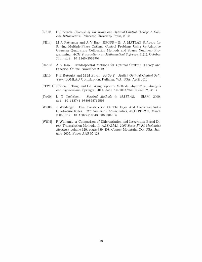
[Lib12] D Liberzon. Calculus of Variations and Optimal Control Theory: A Con-cise Introduction. Princeton University Press, 2012.

[PR14] M A Patterson and A V Rao. GPOPS− II: A MATLAB Software forSolving Multiple-Phase Optimal Control Problems Using hp-AdaptiveGaussian Quadrature Collocation Methods and Sparse Nonlinear Pro-gramming. ACM Transactions on Mathematical Software, 41(1), October2014. doi: 10.1145/2558904

[Rao12] A V Rao. Pseudospectral Methods for Optimal Control: Theory andPractice. Online, November 2012.

[RE10] P E Rutquist and M M Edvall. PROPT - Matlab Optimal Control Soft-ware. TOMLAB Optimization, Pullman, WA, USA, April 2010.

[STW11] J Shen, T Tang, and L-L Wang. Spectral Methods: Algorithms, Analysisand Applications. Springer, 2011. doi: 10.1007/978-3-540-71041-7

[Tre00] L N Trefethen. Spectral Methods in MATLAB. SIAM, 2000.doi: 10.1137/1.9780898719598

[Wal06] J Waldvogel. Fast Construction Of The Fejer And Clenshaw-CurtisQuadrature Rules. BIT Numerical Mathematics, 46(1):195–202, March2006. doi: 10.1007/s10543-006-0045-4

[Wil05] P Williams. A Comparison of Differentiation and Integration Based Di-rect Transcription Methods. In AAS/AIAA 2005 Space Flight MechanicsMeetings, volume 120, pages 389–408, Copper Mountain, CO, USA, Jan-uary 2005. Paper AAS 05-128.

18

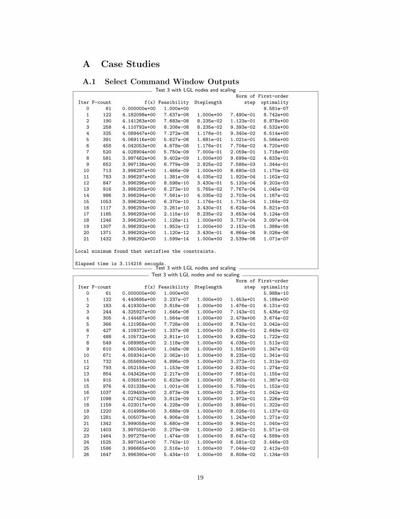
A Case Studies

A.1 Select Command Window OutputsTest 3 with LGL nodes and scaling

Norm of First-order

Iter F-count f(x) Feasibility Steplength step optimality

0 61 0.000000e+00 1.000e+00 9.581e-07

1 122 4.182098e+00 7.637e-08 1.000e+00 7.490e-01 8.742e+00

2 190 4.141263e+00 7.683e-08 8.235e-02 1.123e-01 8.878e+00

3 258 4.110792e+00 8.208e-08 8.235e-02 9.393e-02 6.532e+00

4 325 4.089447e+00 7.272e-08 1.176e-01 9.340e-02 6.514e+00

5 391 4.069116e+00 5.627e-08 1.681e-01 1.021e-01 5.566e+00

6 458 4.042053e+00 4.678e-08 1.176e-01 7.704e-02 4.720e+00

7 520 4.028904e+00 5.750e-09 7.000e-01 2.059e-01 1.718e+00

8 581 3.997462e+00 9.402e-09 1.000e+00 9.699e-02 4.633e-01

9 652 3.997136e+00 6.779e-09 2.825e-02 7.586e-03 1.344e-01

10 713 3.996297e+00 1.466e-09 1.000e+00 8.680e-03 1.170e-02

11 783 3.996297e+00 1.381e-09 4.035e-02 1.920e-04 1.162e-02

12 847 3.996296e+00 8.598e-10 3.430e-01 5.120e-04 9.202e-03

13 916 3.996295e+00 8.273e-10 5.765e-02 7.767e-04 1.045e-02

14 986 3.996294e+00 7.561e-10 4.035e-02 2.703e-04 1.167e-02

15 1053 3.996294e+00 6.370e-10 1.176e-01 1.713e-04 1.164e-02

16 1117 3.996293e+00 3.261e-10 3.430e-01 6.624e-04 5.821e-03

17 1185 3.996293e+00 2.115e-10 8.235e-02 3.653e-04 5.124e-03

18 1246 3.996292e+00 1.128e-11 1.000e+00 3.737e-04 3.097e-04

19 1307 3.996292e+00 1.952e-12 1.000e+00 2.152e-05 1.388e-05

20 1371 3.996292e+00 1.120e-12 3.430e-01 6.864e-06 9.026e-06

21 1432 3.996292e+00 1.599e-14 1.000e+00 2.539e-06 1.071e-07

Local minimum found that satisfies the constraints.

Elapsed time is 3.114216 seconds.Test 3 with LGL nodes and scaling

Test 3 with LGL nodes and no scalingNorm of First-order

Iter F-count f(x) Feasibility Steplength step optimality

0 61 0.000000e+00 1.000e+00 5.988e-10

1 122 4.440695e+00 2.237e-07 1.000e+00 1.453e+01 5.188e+00

2 183 4.419303e+00 3.818e-09 1.000e+00 1.476e-01 6.131e-02

3 244 4.325927e+00 1.646e-08 1.000e+00 7.143e-01 5.436e-02

4 305 4.144487e+00 1.564e-08 1.000e+00 2.479e+00 3.674e-02

5 366 4.121958e+00 7.728e-09 1.000e+00 8.743e-01 3.042e-02

6 427 4.109372e+00 1.337e-08 1.000e+00 3.636e-01 2.649e-02

7 488 4.105732e+00 2.811e-10 1.000e+00 9.628e-02 1.722e-02

8 549 4.089985e+00 2.118e-09 1.000e+00 4.036e-01 1.512e-02

9 610 4.060340e+00 1.048e-08 1.000e+00 1.552e+00 1.347e-02

10 671 4.059341e+00 2.062e-10 1.000e+00 8.235e-02 1.341e-02

11 732 4.055693e+00 4.896e-09 1.000e+00 3.272e-01 1.312e-02

12 793 4.052156e+00 1.153e-09 1.000e+00 2.833e-01 1.274e-02

13 854 4.043426e+00 2.217e-09 1.000e+00 7.581e-01 1.155e-02

14 915 4.035815e+00 5.623e-09 1.000e+00 7.955e-01 1.387e-02

15 976 4.031338e+00 1.001e-08 1.000e+00 5.709e-01 1.152e-02

16 1037 4.029493e+00 2.673e-09 1.000e+00 2.265e-01 1.042e-02

17 1098 4.027423e+00 3.812e-09 1.000e+00 1.972e-01 1.226e-02

18 1159 4.023017e+00 4.228e-09 1.000e+00 3.884e-01 1.322e-02

19 1220 4.014998e+00 3.688e-09 1.000e+00 8.026e-01 1.137e-02

20 1281 4.005079e+00 4.906e-09 1.000e+00 1.243e+00 1.271e-02

21 1342 3.999058e+00 5.680e-09 1.000e+00 9.945e-01 1.040e-02

22 1403 3.997552e+00 3.279e-09 1.000e+00 2.982e-01 5.571e-03

23 1464 3.997276e+00 1.474e-09 1.000e+00 8.647e-02 4.589e-03

24 1525 3.997041e+00 7.742e-10 1.000e+00 6.581e-02 3.446e-03

25 1586 3.996665e+00 2.516e-10 1.000e+00 7.044e-02 2.412e-03

26 1647 3.996390e+00 5.434e-10 1.000e+00 8.808e-02 1.134e-03

19

27 1708 3.996302e+00 3.210e-10 1.000e+00 8.893e-02 3.904e-04

28 1769 3.996293e+00 5.595e-11 1.000e+00 3.081e-02 1.640e-04

29 1830 3.996293e+00 2.836e-11 1.000e+00 3.790e-03 1.501e-04

30 1891 3.996293e+00 1.701e-11 1.000e+00 9.169e-04 1.450e-04

31 1952 3.996292e+00 2.365e-11 1.000e+00 1.923e-03 7.148e-05

32 2013 3.996292e+00 1.610e-11 1.000e+00 1.489e-03 2.976e-05

33 2074 3.996292e+00 2.446e-11 1.000e+00 1.060e-03 8.578e-06

34 2135 3.996292e+00 1.545e-12 1.000e+00 2.881e-04 1.519e-06

35 2196 3.996292e+00 1.644e-12 1.000e+00 4.163e-05 9.324e-08

Local minimum found that satisfies the constraints.

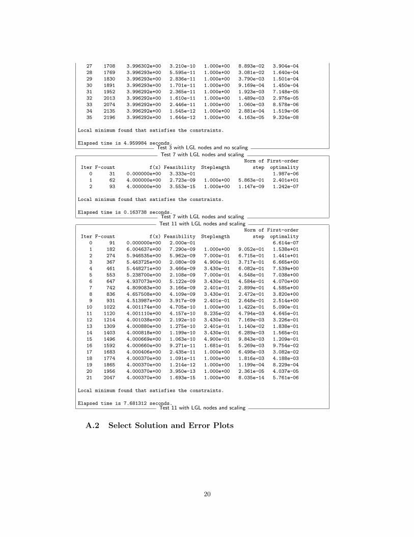
Elapsed time is 4.959984 seconds.Test 3 with LGL nodes and no scaling

Test 7 with LGL nodes and scalingNorm of First-order

Iter F-count f(x) Feasibility Steplength step optimality

0 31 0.000000e+00 3.333e-01 1.987e-06

1 62 4.000000e+00 2.723e-09 1.000e+00 5.863e-01 2.401e+01

2 93 4.000000e+00 3.553e-15 1.000e+00 1.147e-09 1.242e-07

Local minimum found that satisfies the constraints.

Elapsed time is 0.163738 seconds.Test 7 with LGL nodes and scaling

Test 11 with LGL nodes and scalingNorm of First-order

Iter F-count f(x) Feasibility Steplength step optimality

0 91 0.000000e+00 2.000e-01 6.614e-07

1 182 6.004637e+00 7.290e-09 1.000e+00 9.052e-01 1.538e+01

2 274 5.946535e+00 5.962e-09 7.000e-01 6.715e-01 1.441e+01

3 367 5.463725e+00 2.080e-09 4.900e-01 3.717e-01 6.665e+00

4 461 5.448271e+00 3.466e-09 3.430e-01 6.082e-01 7.539e+00

5 553 5.238700e+00 2.108e-09 7.000e-01 4.548e-01 7.038e+00

6 647 4.937073e+00 5.122e-09 3.430e-01 4.584e-01 4.070e+00

7 742 4.809083e+00 3.166e-09 2.401e-01 2.899e-01 4.585e+00

8 836 4.657508e+00 4.109e-09 3.430e-01 2.472e-01 3.820e+00

9 931 4.513987e+00 3.917e-09 2.401e-01 2.648e-01 2.514e+00

10 1022 4.001174e+00 4.705e-10 1.000e+00 1.422e-01 5.090e-01

11 1120 4.001110e+00 4.157e-10 8.235e-02 4.794e-03 4.645e-01

12 1214 4.001038e+00 2.192e-10 3.430e-01 7.169e-03 3.226e-01

13 1309 4.000880e+00 1.275e-10 2.401e-01 1.140e-02 1.838e-01

14 1403 4.000818e+00 1.199e-10 3.430e-01 6.289e-03 1.565e-01

15 1496 4.000669e+00 1.063e-10 4.900e-01 9.843e-03 1.209e-01

16 1592 4.000660e+00 9.271e-11 1.681e-01 5.269e-03 9.754e-02

17 1683 4.000406e+00 2.435e-11 1.000e+00 6.498e-03 3.082e-02

18 1774 4.000370e+00 1.091e-11 1.000e+00 1.816e-03 4.188e-03

19 1865 4.000370e+00 1.214e-12 1.000e+00 1.199e-04 8.229e-04

20 1956 4.000370e+00 3.950e-13 1.000e+00 2.361e-05 4.037e-05

21 2047 4.000370e+00 1.693e-15 1.000e+00 8.035e-14 5.761e-06

Local minimum found that satisfies the constraints.

Elapsed time is 7.681312 seconds.Test 11 with LGL nodes and scaling

A.2 Select Solution and Error Plots

20

x[m

],v[m

/s]

−1

−0.5

0

0.5

1

0 0.25 0.5 0.75 1

t (s)

u[m

/s2]

xinterp vinterp uinterp xLGL vLGL uLGL

0

−2

−4

−6

absolute

error

10−15

10−10

10−5

100

0 0.25 0.5 0.75 1

t (s)

error x error v error u

(a) Test 1, LGL nodes.

x[m

],v[m

/s]

−1

−0.5

0

0.5

1

0 0.25 0.5 0.75 1

t (s)

u[m

/s2]

xinterp vinterp uinterp xLGL vLGL uLGL

0

−2

−4

−6

absolute

error

10−15

10−10

10−5

100

0 0.25 0.5 0.75 1

t (s)

error x error v error u

(b) Test 3, LGL nodes.

x[m

],v[m

/s]

−1

−0.5

0

0.5

1

0 0.25 0.5 0.75 1

t (s)

u[m

/s2]

xinterp vinterp uinterp xLGL vLGL uLGL

0

−2

−4

−6

absolute

error

10−15

10−10

10−5

100

0 0.25 0.5 0.75 1

t (s)

error x error v error u

(c) Test 5, LGL nodes.

Figure 2 Solution and error plots for tests {1, 3, 5} with LGL nodes.

21

x[m

],v[m

/s]

−1

−0.5

0

0.5

1

0 0.25 0.5 0.75 1

t (s)

u[m

/s2]

xinterp vinterp uinterp xLGL vLGL uLGL

0

−2

−4

−6

absolute

error

10−15

10−10

10−5

100

0 0.25 0.5 0.75 1

t (s)

error x error v error u

(a) Test 7, LGL nodes.

x[m

],v[m

/s]

−1

−0.5

0

0.5

1

0 0.25 0.5 0.75 1

t (s)

u[m

/s2]

xinterp vinterp uinterp xLGL vLGL uLGL

0

−2

−4

−6

absolute

error

10−15

10−10

10−5

100

0 0.25 0.5 0.75 1

t (s)

error x error v error u

(b) Test 11, LGL nodes.

x[m

],v[m

/s]

−1

−0.5

0

0.5

1

0 0.25 0.5 0.75 1

t (s)

u[m

/s2]

xinterp vinterp uinterp xLGL vLGL uLGL

0

−2

−4

−6

absolute

error

10−15

10−10

10−5

100

0 0.25 0.5 0.75 1

t (s)

error x error v error u

(c) Test 13, LGL nodes.

Figure 3 Solution and error plots for tests {7, 11, 13} with LGL nodes.

22

x[m

],v[m

/s]

−1

−0.5

0

0.5

1

0 0.25 0.5 0.75 1

t (s)

u[m

/s2]

xinterp vinterp uinterp xCGL vCGL uCGL

0

−2

−4

−6

absolute

error

10−15

10−10

10−5

100

0 0.25 0.5 0.75 1

t (s)

error x error v error u

(a) Test 7, CGL nodes.

x[m

],v[m

/s]

−1

−0.5

0

0.5

1

0 0.25 0.5 0.75 1

t (s)

u[m

/s2]

xinterp vinterp uinterp xCGL vCGL uCGL

0

−2

−4

−6

absolute

error

10−15

10−10

10−5

100

0 0.25 0.5 0.75 1

t (s)

error x error v error u

(b) Test 11, CGL nodes.

x[m

],v[m

/s]

−1

−0.5

0

0.5

1

0 0.25 0.5 0.75 1

t (s)

u[m

/s2]

xinterp vinterp uinterp xCGL vCGL uCGL

0

−2

−4

−6

absolute

error

10−15

10−10

10−5

100

0 0.25 0.5 0.75 1

t (s)

error x error v error u

(c) Test 13, CGL nodes.

Figure 4 Solution and error plots for tests {7, 11, 13} with CGL nodes.

23

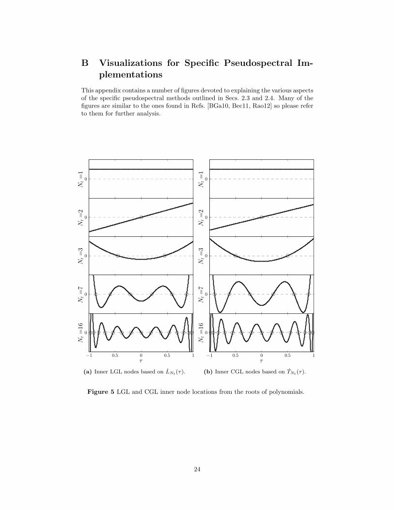
B Visualizations for Specific Pseudospectral Im-plementations

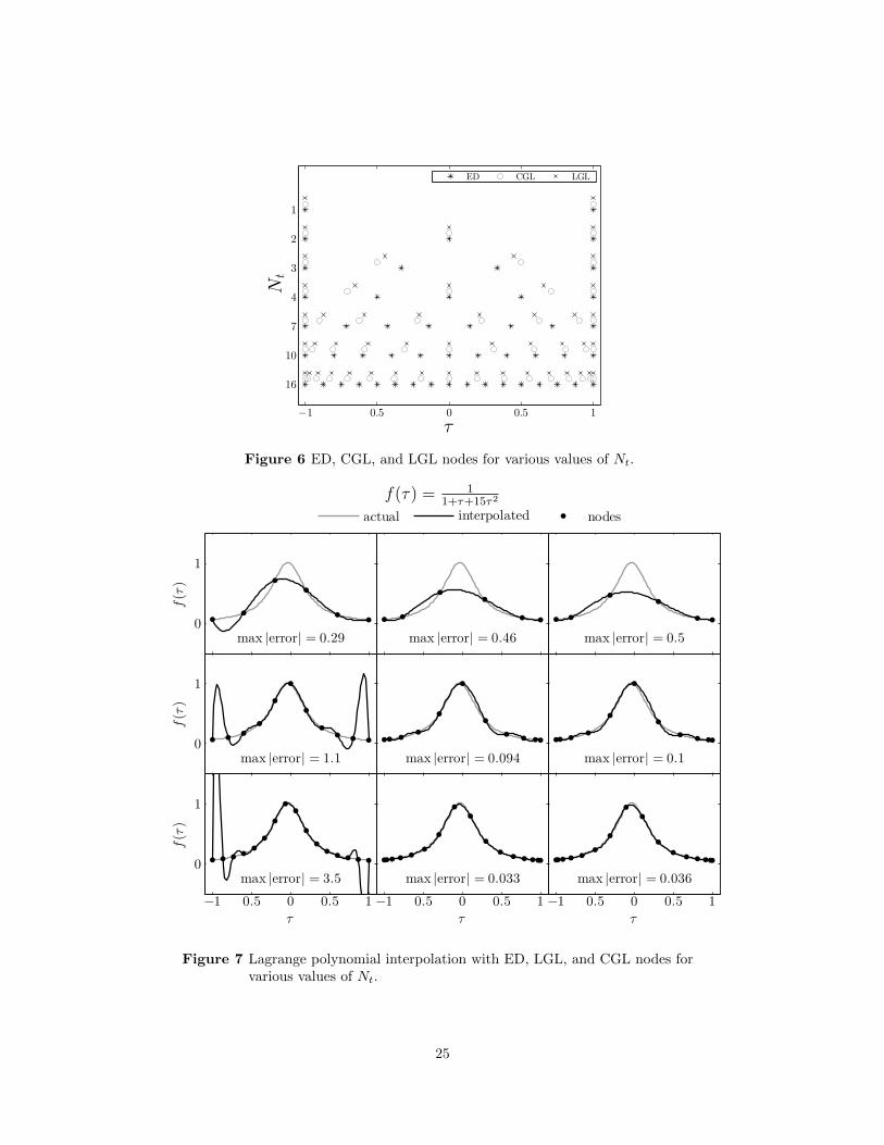
This appendix contains a number of figures devoted to explaining the various aspectsof the specific pseudospectral methods outlined in Secs. 2.3 and 2.4. Many of thefigures are similar to the ones found in Refs. [BGa10, Bec11, Rao12] so please referto them for further analysis.

Nt=1

0

Nt=2

0

Nt=3

0

Nt=7

0

Nt=16

0

−1 0.5 0 0.5 1τ

(a) Inner LGL nodes based on LNt(τ).

Nt=1

0

Nt=2

0

Nt=3

0

Nt=7

0

Nt=16

0

−1 0.5 0 0.5 1τ

(b) Inner CGL nodes based on TNt(τ).

Figure 5 LGL and CGL inner node locations from the roots of polynomials.

24

16

10

7

4

3

2

1

Nt

−1 0.5 0 0.5 1

τ

ED CGL LGL

Figure 6 ED, CGL, and LGL nodes for various values of Nt.

f(τ) = 11+τ+15τ2

0

1

f(τ)

f(τ)

0

1

τ

f(τ)

0

1

−1 0.5 0 0.5 1

τ

−1 0.5 0 0.5 1

τ

−1 0.5 0 0.5 1

actual interpolated nodes

max |error| = 0.29 max |error| = 0.46 max |error| = 0.5

max |error| = 1.1 max |error| = 0.094 max |error| = 0.1

max |error| = 3.5 max |error| = 0.033 max |error| = 0.036

Figure 7 Lagrange polynomial interpolation with ED, LGL, and CGL nodes forvarious values of Nt.

25

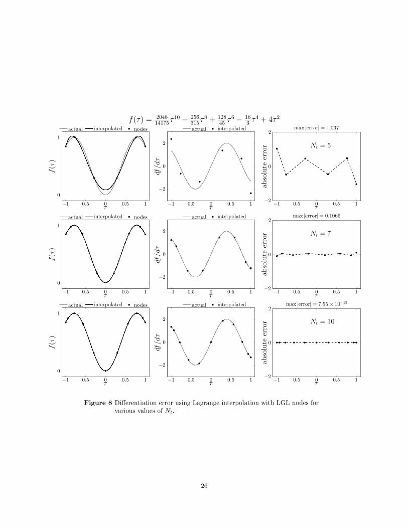
f(τ) = 204814175

τ 10 − 256315τ 8 + 128

45τ 6 − 16

3τ 4 + 4τ 2

0

1

−1 0.5 0 0.5 1τ

f(τ)

actual interpolated nodes

−2

0

2

−1 0.5 0 0.5 1τ

df/dτ

actual interpolated max |error| = 1.037

−2

0

2

−1 0.5 0 0.5 1τ

absolute

error Nt = 5

0

1

−1 0.5 0 0.5 1τ

f(τ)

actual interpolated nodes

−2

0

2

−1 0.5 0 0.5 1τ

df/dτ

actual interpolated max |error| = 0.1065

−2

0

2

−1 0.5 0 0.5 1τ

absolute

error Nt = 7

0

1

−1 0.5 0 0.5 1τ

f(τ)

actual interpolated nodes

−2

0

2

−1 0.5 0 0.5 1τ

df/dτ

actual interpolated max |error| = 7.55 × 10−15

−2

0

2

−1 0.5 0 0.5 1τ

absolute

error Nt = 10

Figure 8 Differentiation error using Lagrange interpolation with LGL nodes forvarious values of Nt.

26

10−16

10−12

10−8

10−4

100

1 10 20 30 40 50 60

Nt

absolute

error

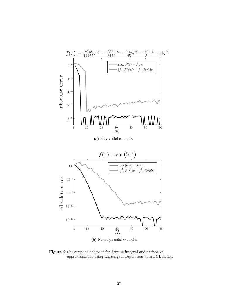
f(τ ) = 204814175τ

10−

256315τ

8 + 12845 τ

6−

163 τ

4 + 4τ 2

max |P (τ)− f(τ)|

|∫ 1

−1 P (τ)dτ −

∫ 1

−1 f (τ)dτ |

(a) Polynomial example.

10−16

10−12

10−8

10−4

100

1 10 20 30 40 50 60

Nt

absolute

error

f(τ ) = sin(

5τ 2)

max |P (τ)− f(τ)|

|∫ 1

−1 P (τ)dτ −

∫ 1

−1 f (τ)dτ |

(b) Nonpolynomial example.

Figure 9 Convergence behavior for definite integral and derivativeapproximations using Lagrange interpolation with LGL nodes.

27

C Supplementary MATLABr Code

The code used in the numeric case studies is available at:http://www.mathworks.com/matlabcentral/fileexchange/51104

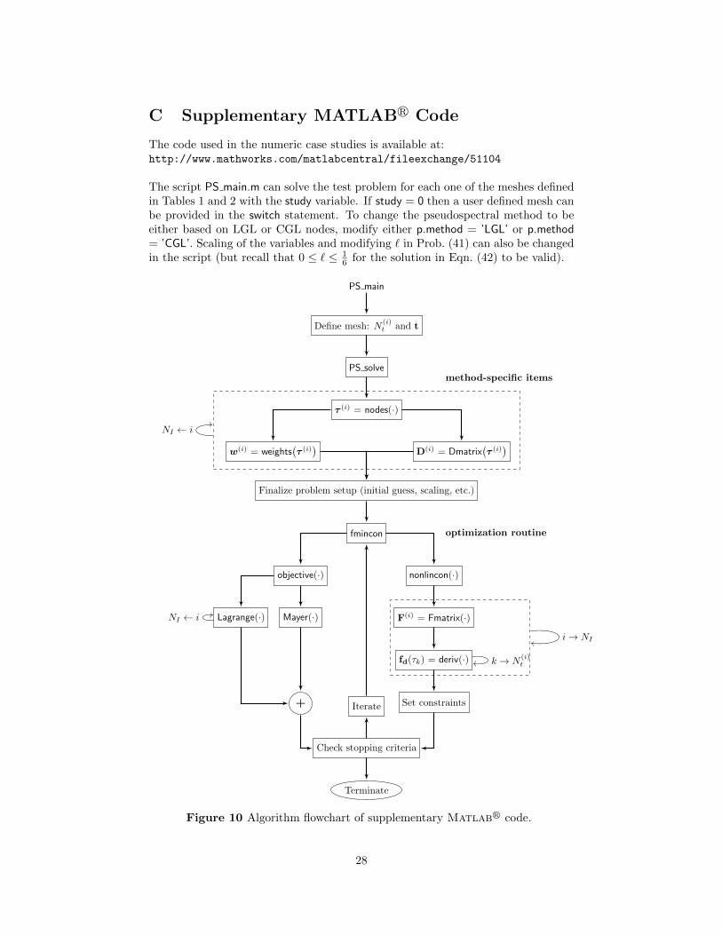
The script PS main.m can solve the test problem for each one of the meshes definedin Tables 1 and 2 with the study variable. If study = 0 then a user defined mesh canbe provided in the switch statement. To change the pseudospectral method to beeither based on LGL or CGL nodes, modify either p.method = ’LGL’ or p.method= ’CGL’. Scaling of the variables and modifying ` in Prob. (41) can also be changedin the script (but recall that 0 ≤ ` ≤ 1

6 for the solution in Eqn. (42) to be valid).

PS main

Define mesh: N(i)t and t

PS solve

τ (i) = nodes(·)

w(i) = weights(τ (i)

)D(i) = Dmatrix

(τ (i)

)

Finalize problem setup (initial guess, scaling, etc.)

fmincon

objective(·) nonlincon(·)

Mayer(·)Lagrange(·)

+

Check stopping criteria

Iterate

Terminate

F(i) = Fmatrix(·)

fd(τk) = deriv(·)

Set constraints

optimization routine

method-specific items

NI ← i

NI ← i

i→ NI

k → N(i)t

Figure 10 Algorithm flowchart of supplementary Matlabr code.

28