BASIC PRINCIPLESOF MR IMAGING

GE Medical SystemsTraining in Partnership

In addition to the built-in features of the Adobe Acrobat™ Reader software, several different types of navigation devices have been added to this electronicdocument. These “buttons” will appear at various points within the documentand allow you to jump to specific reference areas. A brief explanation of thesebuttons is illustrated below:

NAVIGATION NOTES ON USING THIS ELECTRONIC DOCUMENT

CONTINUED

BACK

(FIG. 58)

This button will appear in the lower right corner of ascreen containing text. It means that the next few pagesare going to be images or illustrations. By clicking thecursor on this button you will be taken to the next pagein the current text chain.

This button appears within the text itself. If a particularfigure (either an illustration or an image) is being refer-enced — then clicking the cursor on the colored text willtake you to the page containing that particular figure.

This button works in tandem with the (FIG) button.It appears on the bottom of a page containing anillustration or image. Clicking on it will return you tothe portion of text that the figure was referenced from.

BASIC PRINCIPLES OFMAGNETIC RESONANCE IMAGING

COPYRIGHT© 1990GENERAL ELECTRIC COMPANY

PAUL J. KELLER, PH.D.

DEPARTMENT OF MAGNETIC RESONANCE RESEARCH

BARROW NEUROLOGIC INSTITUTE

ST. JOSEPH’S HOSPITAL AND MEDICAL CENTER

PHOENIX, AZ 85013

TABLE OF CONTENTSFOREWORD . . . . . . . . . . . . . . . . . . . . . . . . . . . . . . . . . . . . . . . . . . . . . . . . . . . . . . . . . . . . . . . . . . . . . . . . . . . . .5BASICS OF THE MAGNETIC RESONANCE PHENOMENON . . . . . . . . . . . . . . . . . . . . . . . . . . . . . . . . . . . . . . . . . . .6

Spins in a Magnetic Field . . . . . . . . . . . . . . . . . . . . . . . . . . . . . . . . . . . . . . . . . . . . . . . . . . . . . . . . . . . . . . . . . . . . . . .7The Effect of Radio Frequency (RF) Pulses . . . . . . . . . . . . . . . . . . . . . . . . . . . . . . . . . . . . . . . . . . . . . . . . . . . . . . . .15Relaxation: The Return to Equilibrium . . . . . . . . . . . . . . . . . . . . . . . . . . . . . . . . . . . . . . . . . . . . . . . . . . . . . . . . . . .16

TRANSVERSE RELAXATION . . . . . . . . . . . . . . . . . . . . . . . . . . . . . . . . . . . . . . . . . . . . . . . . . . . . . . . . . . . . . . . . . . .20LONGITUDINAL RELAXATION . . . . . . . . . . . . . . . . . . . . . . . . . . . . . . . . . . . . . . . . . . . . . . . . . . . . . . . . . . . . . . . . .24FACTORS INFLUENCING RELAXATION RATES . . . . . . . . . . . . . . . . . . . . . . . . . . . . . . . . . . . . . . . . . . . . . . . . . . . . . .27

The Effect of Magnetic Field Gradients . . . . . . . . . . . . . . . . . . . . . . . . . . . . . . . . . . . . . . . . . . . . . . . . . . . . . . . . . . .30Fourier Transformation . . . . . . . . . . . . . . . . . . . . . . . . . . . . . . . . . . . . . . . . . . . . . . . . . . . . . . . . . . . . . . . . . . . . . . .34

PRINICIPLES AND TECHNIQUES IN MR IMAGING . . . . . . . . . . . . . . . . . . . . . . . . . . . . . . . . . . . . . . . . . . . . . . .37Instrumentation . . . . . . . . . . . . . . . . . . . . . . . . . . . . . . . . . . . . . . . . . . . . . . . . . . . . . . . . . . . . . . . . . . . . . . . . . . . . .37

THE B0 FIELD . . . . . . . . . . . . . . . . . . . . . . . . . . . . . . . . . . . . . . . . . . . . . . . . . . . . . . . . . . . . . . . . . . . . . . . . . . .37MAGNETIC FIELD GRADIENTS . . . . . . . . . . . . . . . . . . . . . . . . . . . . . . . . . . . . . . . . . . . . . . . . . . . . . . . . . . . . . . . .40THE B1 FIELD . . . . . . . . . . . . . . . . . . . . . . . . . . . . . . . . . . . . . . . . . . . . . . . . . . . . . . . . . . . . . . . . . . . . . . . . . . .42THE RECEIVER . . . . . . . . . . . . . . . . . . . . . . . . . . . . . . . . . . . . . . . . . . . . . . . . . . . . . . . . . . . . . . . . . . . . . . . . . . .44THE COMPUTER SYSTEM . . . . . . . . . . . . . . . . . . . . . . . . . . . . . . . . . . . . . . . . . . . . . . . . . . . . . . . . . . . . . . . . . . . .46

Slice Selective Excitation . . . . . . . . . . . . . . . . . . . . . . . . . . . . . . . . . . . . . . . . . . . . . . . . . . . . . . . . . . . . . . . . . . . . . .47Frequency Encoding . . . . . . . . . . . . . . . . . . . . . . . . . . . . . . . . . . . . . . . . . . . . . . . . . . . . . . . . . . . . . . . . . . . . . . . . . .52Phase Encoding . . . . . . . . . . . . . . . . . . . . . . . . . . . . . . . . . . . . . . . . . . . . . . . . . . . . . . . . . . . . . . . . . . . . . . . . . . . . .57Reconstruction . . . . . . . . . . . . . . . . . . . . . . . . . . . . . . . . . . . . . . . . . . . . . . . . . . . . . . . . . . . . . . . . . . . . . . . . . . . . . .61Multislice Acquisition . . . . . . . . . . . . . . . . . . . . . . . . . . . . . . . . . . . . . . . . . . . . . . . . . . . . . . . . . . . . . . . . . . . . . . . . .65Contrast . . . . . . . . . . . . . . . . . . . . . . . . . . . . . . . . . . . . . . . . . . . . . . . . . . . . . . . . . . . . . . . . . . . . . . . . . . . . . . . . . . .67Parameters Influencing the Signal-to-Noise Ratio (SNR) and Spatial Resolution . . . . . . . . . . . . . . . . . . . . . . . . . . . .72Imaging with Gradient Echoes . . . . . . . . . . . . . . . . . . . . . . . . . . . . . . . . . . . . . . . . . . . . . . . . . . . . . . . . . . . . . . . . . .783D-Gradient Echo Imaging . . . . . . . . . . . . . . . . . . . . . . . . . . . . . . . . . . . . . . . . . . . . . . . . . . . . . . . . . . . . . . . . . . . . .84

BIBLIOGRAPHY . . . . . . . . . . . . . . . . . . . . . . . . . . . . . . . . . . . . . . . . . . . . . . . . . . . . . . . . . . . . . . . . . . . . . . . . .90GLOSSARY . . . . . . . . . . . . . . . . . . . . . . . . . . . . . . . . . . . . . . . . . . . . . . . . . . . . . . . . . . . . . . . . . . . . . . . . . . . . .93

FOREWORDDr. Paul Keller, the author of the currentprimer, has a profound understanding ofmagnetic resonance and its many applications,and many years of hands-on experience.Beyond this, he has the rare ability to teachMR physics (a term for which the averageradiologist has an innate aversion) in a non-threatening and lucid manner.

Felix W. WehrliMilwaukee, WisconsinJune, 1988

For many MR users, “NMR: A Perspectiveon Imaging” had been the first exposure tomagnetic resonance. This highly successfulprimer was reprinted twice, and is nowpermanently out of print. Why not reprintit a third time? After all, MR physics cannothave changed a great deal over the past sixyears. True, but our understanding has,and so has the significance of many of itsaspects. In fact, the technology has madetremendous leaps forward since the begin-ning of this decade, when MR entered thephase of initial clinical trials. Also, theunderstanding of critical performance criteriahas become more sophisticated, parallelingadvances in instrumentation. New method-ology, such as rapid imaging, 3D acquisition,variable bandwidth and many more areterms and techniques which confront theMR novice.

CONTINUED

Over the past several years, magnetic resonanceimaging (MRI) has developed into a verypowerful and versatile diagnostic techniquein medicine. This, in turn, led to the prolifera-tion of MRI equipment and spurred massiveamounts of research.

What are the reasons for all of this excitement?Unlike x-ray based modalities such as computedtomography (CT) scanning, MRI is a non-invasive technique which does not employionizing radiation. Further, the only tissue-specific parameter that can be determinedwith x-rays is electron density, which doesnot vary greatly from one soft tissue toanother, and often necessitates the injectionof contrast media.

In MRI, on the other hand, there is a multitudeof tissue parameters which can affect MRsignals. The two most significant, the relax-ation times, cover a wide range of values invarious normal and pathologic tissues.In addition, signal acquisition parameterscan be manipulated in a variety of ways,enabling the user to control image contrast.

This primer has been written for physiciansand technologists who seek an introductionto the mechanisms underlying MRI.

The first section discusses the physics ofmagnetic resonance of atomic nuclei. Thesecond section introduces the techniquesemployed for exploiting the MR phenomenonfor the purpose of image formation.

C H A P T E R 1

CHAPTER 1

BASICS OF THE MAGNETICRESONANCE PHENOMENON

CONTINUED

A few basic physical equations are provided,but the text can be largely understood with-out them. Many of the figures and much ofthe glossary have been borrowed from anearlier primer published by GE Medical Systems.

SPINS IN A MAGNETIC FIELD

During the development of the quantummechanical concept of atomic structure, itbecame apparent that most nuclei possessa property called spin angular momentum,which is the basis of nuclear magnetism.In the following, let us construct an intuitiveview of the consequences and manipulationof nuclear spin. (REFS. 14-15).

(FIG. 1) depicts a nucleus spinning aroundan axis. Since atomic nuclei are charged,the spinning motion causes a magneticmoment which is colinear with the directionof the spin axis. The magnetic moment actssimilar to a bar magnet having north andsouth poles. The strength of this magneticmoment is a property of the type of nucleusand determines the detection sensitivity ofMR (TABLE 1). 1H nuclei (protons) possessthe strongest magnetic moment, which,

together with the high biological abundanceof hydrogen, makes it the nucleus of choicefor MR imaging.

Consider a collection of protons as in (FIG. 2).In the absence of an externally applied magneticfield, the individual magnetic moments haveno preferred orientation. However, if anexternally supplied magnetic field (denotedB0) is imposed, there is a tendency for themagnetic moments to align with the externalfield, just like bar magnets would do. Nuclearmagnetic moments in this situation mayadopt one of two possible orientations:alignment parallel or anti-parallel to B0 (FIG. 3).Thus, depending on their orientation, wecan define two groups or populations ofspins. Alignment parallel to B0 is the lowerenergy orientation and is thus preferred,while the anti-parallel alignment is the higherenergy state (FIG. 4). For the sake of com-pleteness, it should be mentioned that thissituation of only two allowed states is trueonly for nuclei whose “magnetic spin quantumnumber” is equal to 1/2. This includes 1H,13C, 19F, 31P and others.

C H A P T E R1

CONTINUED

FIGURE 1 – The magnetic dipole and associated spin of certain nuclei maybe compared to a common bar magnet with rotation about the dipole axis.

C H A P T E R 1

BACK

���������yyyyzz{{|

N

S

TABLE 1 – Magnetic Resonance properties of some biochemically important nuclei

C H A P T E R1

BACK

1 Gamma is directly proportional to the magnitude of the nuclear magnetic moment. 2 At constant field for equal numbers of nuclei.

NATURAL GAMMA1 RELATIVE2NUCLEUS ABUNDANCE % HZ / GAUSS SENSITIVITY

1H 99.98 4257 12H 0.015 653 0.009713C 1.1 1071 0.01619F 100 4005 0.830

23Na 100 1126 0.09331P 100 1723 0.06639K 93.1 199 0.0005

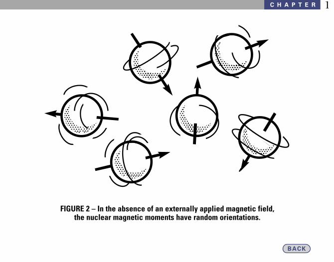
FIGURE 2 – In the absence of an externally applied magnetic field,the nuclear magnetic moments have random orientations.

C H A P T E R 1

BACK

������yz{{||������yyzz{|��

����yz{{||������yz{{||����yz{| ������yyzz{|

FIGURE 3 – In the presence of an externally applied magnetic field (B0) spinsare constrained to adopt one of two orientations with respect to B0. These

orientations are denoted as parallel and anti-parallel.

C H A P T E R1

BACK

������yyz{{|

������yyz{{|

θ

B0

Parallel

Antiparallel

FIGURE 4 – The parallel spin orientation is a lower energy state than anti parallel.Since spins must adopt one of the two orientations, there are two populations

(P1, P2) of spins corresponding to two energy levels (E1, E2). E2 is greater than E1,causing P1 to be greater than P2. Some spins of P1 may move to P2 if the exact

amount of energy equal to E2 - E1 = ∆E is supplied to the system.

C H A P T E R 1

BACK

Parallel

Antiparallel

IncreasingEnergy

E2

E1 p1

p2

∆E

Other magnetically active nuclei, e.g. 2H and23Na, are allowed more than two orientations.

One might think that all of the spins wouldoccupy the lower energy state. This wouldbe true at a temperature of absolute zero,but we are interested in the situation undersomewhat more temperate conditions. Sincethe energy difference (∆K) between the twostates is very small, thermal energy alonecauses the two states to be almost equallypopulated (the population ratio is approxi-mately 100,000 to 100,006). The remainingpopulation difference results in a net bulkmagnetization aligned parallel to B0. It is onlythis net magnetization arising from a smallpopulation difference which is detectable byMR techniques.

Let’s examine this net magnetization inmore detail. The individual spins do notalign exactly parallel (or antiparallel) to B0,but at an angle to B0 (FIG. 5A). The spinassociated with the magnetic moment causesthe moment to precess around the axis ofB0. This is analogous to the case of a spinningtop: the top precesses about the axis defined

by the pull of gravity. This precession thendefines the surface of a cone.

Now we may refine our picture of how alarge collection of spins yields a net bulkmagnetization. (FIG. 5B) shows a model of thesituation at any given instant. Here, each ofthe vectors (arrows) represents an individualspin. Since we already know that there aremore spins aligned with B0 than against B0,the contribution of the bottom cone cancelsout, leaving only the excess spins of the topcone to consider. Any given vector on thetop cone could be described by its componentsperpendicular to and parallel to B0. Clearly,for a large enough collection of spins randomlydistributed on the surface of the cone, individualcomponents perpendicular to B0 will canceleach other. This leaves only the contributionsparallel to B0 explaining why the bulk netmagnetization is indeed parallel to B0.

We may next inquire how fast the individualspins precess on the surface of the cone.

C H A P T E R1

CONTINUED

FIGURE 5 – (A) As seen previously in FIGURE 3, the spin axes do not actually align par-allel or anti-parallel to B0, but at an angle to B0. This causes the spin axis to precesslike a top around B0, thus describing the surface of a cone. (B) This is a depiction of acollection of spins at any given instant. The vector (arrow) M represents the bulk netmagnetization which results from the sum of the contributions from each of the spins.

C H A P T E R 1

BACK

B0 B0

Parallel

Antiparallel

M

This precessional frequency is given by abeautifully simple relationship called theLarmor equation, expressed as:

[1] γB0 = F

F is the precessional frequency, B0 is thestrength of the magnetic field, and gamma(γ) is related to the strength of the magneticmoment for the type of nucleus considered.

For our purposes:

γH = 4257 Hz / Gauss

Thus at 1.5 Tesla (= 15,000 Gauss) 4257 Hz/Gauss x 15,000 Gauss = 63,855,000 Hertz =63.855 Megahertz (MHz).

Correspondingly, at 0.5 Tesla, the Larmorfrequency for protons is 21.285 MHz. Wesee that the rate of precession is very fast.

Re-examination of (FIG. 4) shows that sinceenergy is proportional to frequency, ∆E maybe defined in terms of the frequency ofradiation which is necessar y to induce

transitions of spins between the two energylevels. For reasons which are not obviouswithout delving more deeply into physics,the frequency corresponding to ∆E is againthe Larmor frequency.

THE EFFECT OF RADIOFREQUENCY (RF) PULSES

In order to detect a signal, a condition ofresonance needs to be established. The term“resonance” implies alternating absorptionand dissipation of energy. Energy absorptionis caused by RF perturbation, and energydissipation is mediated by relaxation processes(Next Section). Simply put, as mentionedabove, irradiation of a collection of spins inan exogenous magnetic field with RF energyat the Larmor frequency induces transitionsbetween the two energy levels. RF energy atother frequencies has no effect. That isthe microscopic picture, but what canactually be observed for the macroscopicnet magnetization?

C H A P T E R1

CONTINUED

RF radiation, like all electromagnetic radia-tion, possesses electric and magnetic fieldcomponents. We may consider the RF asanother magnetic field (denoted as B1)perpendicular to B0, i.e. along a given axisin the transverse plane (FIG. 6). When theRF is turned on, the net magnetization vectorbegins to precess about the B1 axis. Thus thenet magnetization rotates from the longitudinal(Z) axis toward the transverse plane thentoward the –Z axis, then to the other side ofthe transverse plane, and back to +Z and soon. If the RF is on for only a short period oftime, the net magnetization is rotated by acertain angle away from the longitudinalaxis; this angle is termed the flip angle.Intuitively, we understand that the flip angleis proportional to the duration of an RFpulse and the amplitude of the RF. As wewill see, flip angles of 90° and 180° are ofspecial importance in imaging.

Consider the situation immediately after a90° pulse (FIG. 7). The net magnetizationnow lies in the transverse plane and beginsto precess around the B0 axis. The rate ofthis precession is just as calculated above—

it is the Larmor frequency. Since this ismacroscopic magnetization which is changingdirection (rotating) over time, it can inducean alternating (AC) current in a coil of wire,and that current can be used to record theaction of magnetization in the transverseplane. (FIG. 8) shows such a record. Notethat it shows a sinusoidal oscillation at theLarmor frequency. Furthermore, the signalgets weaker with time. This is a free inductiondecay (or FID). Here “free” refers to thelack of the driving B1 field at the time ofobservation; the signal which is induced inthe receiver coil decays over time. The signaldecay is due to a process known as relaxation.

RELAXATION: THE RETURN TO EQUILIBRIUM

Returning briefly to the analogy of a barmagnet aligned with an external magneticfield, we may inquire about what happens ifthe bar magnet is turned away from thisalignment. The bar magnet would naturallytend to realign itself with the field, but howrapidly would this occur?

C H A P T E R 1

CONTINUED

FIGURE 6 – RF energy at the Larmor frequency acts as a second magnetic field (B1)which is perpendicular to B0. When the RF is on, M rotates about B1. As shown here,M is originally longitudinal and B1 is turned on long enough to rotate M by 90° i.e..

into the transverse plane.

C H A P T E R1

BACK

B1

B0

M

FIGURE 7 – Once in the transverse plane, M precesses (rotates) about B0 at the Larmorfrequency. This rotating magnetization can induce an AC current in the receiver coil.The transverse magnetization decays over time, which is represented by a decreasing

length of the vector M.

C H A P T E R 1

BACK

MXY

ReceiverCoil

FIGURE 8 – A graph of the voltage (signal) induced in the receiver coil versus time.This waveform is termed a free induction decay (FID); it is an ex ponentially damped

sine wave. The decay rate is characterized by the time constant T2*.

C H A P T E R1

BACK

SignalAmplitude

Time

-t/T2*e

1.0

0.5

0.0

-0.5

-1.0

Would the return to equilibrium be linearor exponential with respect to time? For thebar magnet, the equilibrium orientation isin alignment with the external field. Onceequilibrium conditions have been attainedthere is no further change unless the systemis perturbed.

For the net magnetization arising froma collection of spins in an external fieldequilibrium is described by a vector of unitlength parallel to B0. We will see that it isappropriate to consider relaxation in thetransverse plane independently of relax-ation along the longitudinal axis.

Transverse RelaxationGiven that at equilibrium the net magnetiza-tion is longitudinal, it follows that the equi-librium magnetization in the transverseplane is zero. This is illustrated in (FIG. 8),showing the decay of the transverse magne-tization to zero. This process is exponential(as opposed to linear). This is reminiscentof other natural processes, e.g. radioactivedecay. As in radioactive decay one could

define a quantity such as the half-life for thetransverse magnetization. The relationshipdescribing the decay is

[2] Mtransverse = M0transverse e-t / T2 *

Where M0transverse is the initial amount of

transverse magnetization, Mtransverse is theamount of transverse magnetization at anygiven time (t) after a pulse, e is approximately2.7, and T2* characterizes the rate of decay.

If t = T2*, M(T2*) = M 0transverse / e =

M 0transverse / 2 .7 = 0.37 M 0

transverse •

Hence, T2* is the time it takes for thetransverse magnetization to decay to 37%of the initial value.

What mechanisms cause the observed decayof transverse magnetization? As shown in(FIG. 9), different components of the mag-netization may precess at slightly differentrates, a process known as “dephasing” in thetransverse plane.

C H A P T E R 1

CONTINUED

FIGURE 9 – (A) The B1 field of the RF rotates M into the transverse plane. (B-E) The mag-netization rotating in the transverse plane is actually the sum of the contributions fromall of the spins in the excited sample. However, the spins at different points in the sample

may not “feel” the same B0 field due to B0 inhomogeneity. This results in a range ofprecessional frequencies, causing the various components of M to spread apart overtime. This loss of “phase coherence” eventually leads to self-cancellation of the signal.

C H A P T E R1

BACK

y

y

y

y

yx

xx

xx ω ω

(A) (B) (C)

(D) (E)

Since the signal recorded is the sum of allthe transverse components, sufficient dephas-ing will lead to complete cancellation of thesignal. One of the major causes of this dephas-ing is B0 inhomogeneity: spins at differentlocations are not exposed to exactly the sameB0 field, which in turn yields a range of Larmorfrequencies. If one had a completely homo-geneous B0 field, dephasing would still occur,but much more slowly. Since many atomicnuclei and electrons are spins and possessmagnetic moments, the microscopic localmagnetic environment of a spin participatingin the observed resonance is not preciselyidentical to those of the other observedspins. Additionally, these microscopic envi-ronments change very rapidly. This spatialand temporal variation of magnetic environmentsyields variation in the Larmor frequenciescausing the slower dephasing This slowerdephasing and concomitant signal decay isdue to the physical properties of the system(or tissue) under investigation, and is denotedas T2 relaxation or spin-spin relaxation.Now it can be appreciated that T2* describesthe decay rate observed due to the combinationof spin-spin relaxation and B0 inhomogeneity.

For many reasons it is useful to record signalswhich reflect T2 rather than T2* decay. Obviously,some sort of trick is necessary in order toaccomplish this, since a perfectly homoge-neous B0 field is not attainable. The “trick”is called a spin-echo, and it is the basis forthe majority of clinical MR imaging A pulsesequence is a set of RF pulses (and for imaging,field gradient pulses as introduced in thenext section) of defined timing and amplitudewhich is usually repeated many times, eachtime resulting in collection of an MR signal.(FIG. 10) depicts an RF pulse sequence for aspin-echo. An initial 90° pulse yields a FIDwhich decays as a function of T2*, then at atime TE/2 after the 90° pulse, a 180° RFpulse is applied. After the 180° pulse, a so-called “echo signal” forms, reaching its maximumamplitude at time TE after the initial 90°pulse. A second spin-echo can be obtainedby applying another 180° pulse, and furtherechoes are possible with additional 180° pulses.Note that the echo-to-echo amplitudes decayas a function of T2 rather than T2*.

C H A P T E R 1

CONTINUED

FIGURE 10 – A spin echo is generated by the application of a 90° RF pulse and,after a delay (TE/2), a 180° RF pulse. The peak of the echo occurs at time TE afterthe initial 90° pulse. Further echoes are obtainable with additional 180° pulses.The echo-to-echo decay rate is described by T2, which is much longer than T2*.

C H A P T E R1

BACK

T2 Decay

T2* Decay

Signal

RF

90˚ 180˚

TE/2TE TE

180˚

1st Spin-Echo 2nd Spin-Echo

What causes the echoes to form, and how isthe effect of B0 inhomogeneity eliminated?The mechanism of spin- echo formation canbe explained by reference to (FIG. 11) .Consider transverse magnetization arisingfrom two locations experiencing differentvalues of B0.

Transverse magnetization from the two locationswill precess at different rates. This is symbolizedwith two vectors labeled as F (fast) and S(slow). Immediately after the 90° pulse, Fand S are together (in phase) in the transverseplane. Both F and S begin to precess clock-wise in the plane, but as time goes on F andS get further apart because of their differentprecessional rates. At this time, the 180° RFpulse is applied. Its effect is to rotate both Fand S into mirror image locations relative tothe 180° rotation axis. F and S now continueclockwise precession, with F behind S. Attime (TE), however, F will catch up with Sand both will be back in phase again. Ifthere were many vectors with a wide rangeof precessional frequencies, they would allstill come back into phase at time TE. In thesection on imaging techniques it will become

clear that the choices of TE and TR (timebetween repetitions of the entire pulsesequence) have a significant impact on signaland contrast of MR images. (REF. 16)

Longitudinal RelaxationUp to this point, only relaxation in the trans-verse plane has been discussed. A separateprocess must exist which restores longitudinalmagnetization to its equilibrium value.

Immediately after a 90° pulse, the net mag-netization vector lies in the transverse plane.Therefore the amount of longitudinal mag-netization is zero. If we examine the amountof longitudinal magnetization present atvarious times after the 90° pulse, we findthat it builds up exponentially from zero toapproach the equilibrium value, which is afunction of the number of spins present,temperature and magnetic field strength(FIG. 12). The process by which this occursis denoted as spin-lattice relaxation or T1relaxation. In terms of the two energy levelsin (FIG. 4), a 90° pulse makes the spinpopulations equal.

C H A P T E R 1

CONTINUED

FIGURE 11 – Mechanism of spin echo magnetization which begins to lose phase coher-ence largely due to B0 inhomogeneity. As the magnetization precesses and fans out in

the transverse plane, the fast (F) and slow (S) edges of the magnetization can beidentified. The 180° pulse rotates all of the magnetization up out of the transverse plane

and back down onto the opposite side of the transverse plane. Precession nowcontinues in the same direction as before, but now the fast edge is behind the slow

edge leading to re-phasing and echo formation.

C H A P T E R1

BACK

TransversePlane

time time

time time

Echo

90˚

RF

180 ̊RF Pulse

F

F

F

S

S

S

FIGURE 12 – After a 90° RF pulse, all of the magnetization lies in the transverse plane.T2 processes and B0 inhomogeneity lead to an exponential decay of transverse

magnetization, while longitudinal magnetization increases with time.

C H A P T E R 1

BACK

Longitudinal

Transverse

Time0

0

M

M0

90 ̊RF

Longitudinal relaxation restores the originalequilibrium population difference by returningsome spins to the lower energy state, and inthe process giving up energy to the environ-ment (lattice).

Longitudinal relaxation seems to share someof the features observed for transverse relaxation;both are characterized by exponential evolution.In what may be viewed as complementaryprocesses, transverse magnetization decays,from maximum to zero, while longitudinalmagnetization builds up from zero to maximum.Not surprisingly then, the quantitative expressionfor T1 relaxation looks similar to what wasseen for T2:

[3] Mlongitudinal = M0longitudinal (1 – e –t / T1)

Equation [3] predicts the amount of longitu-dinal magnetization that will be present attime = t (M longitudinal) and the value of T1.T1 is the length of time necessary to decreasethe difference between the current value ofM longitudinal and the equilibrium value by afactor of (1 – 1/e) = (1 – 1/2.7) = 63% . Thisstatement implies that the rate of increase

in longitudinal magnetization is fastestwhen Mlongitudinal is very different from itsequilibrium value. In (FIG. 12), this conceptof a decreasing rate of change over time isseen graphically. Comparing T1 and T2 forany given system, T1 is always greater thanor equal to T2.

Factors Influencing Relaxation RatesWhat physical factors affect the observedrelaxation times? In general, the same con-ditions that shorten (or lengthen) T1 alsoshorten (or lengthen) T2. There may bemore than one mechanism acting to yieldT1 and/or T2 relaxation, in which case theobserved relaxation (T1 or T2) due to thecombined action of mechanisms labeledgenerically as “a, b, c . . .” is given by:

1 1 1 1[4] ———— = — + — + — + . . .

T observe Ta Tb Tc

Due to this sum of reciprocals relationship,the longer the relaxation time, the greaterthe change caused by the introduction ofan additional mechanism on the observedrelaxation time.

C H A P T E R1

CONTINUED

For pure water T1 = T2, whereas in tissuesT1 >> T2. The total range over which T2 canchange in pathological situations is thereforemuch greater. In fact, in edema, for example,T2 may be prolonged several hundred percent.It is for this reason that images highlightingvariations of T2 are most sensitive in detectingpathology (REF. 11). (TABLE 2) gives T1 and T2values encountered in various normal tissues.

The rate of relaxation is strongly influencedby the rate at which the molecules bearingthe protons being observed tumble in solution.Slower tumbling yields faster relaxation(shorter relaxation times). When tumblingis very slow, as in the case of protons cova-lently bound to macromolecules (proteins,nucleic acids, etc.), T2 is so short that theirsignals decay completely between excitationand detection.

In MRI, only “mobile” protons can contributesignals for imaging These mobile protons arein the form of water and some lipids. Sincelipid molecules are larger than water mole-cules, and hence tumble more slowly, in

general, lipid protons relax more quicklythan water protons.

The issue of water relaxation in vivo is com-plicated by the fact that water moleculesspend part of the time freely tumbling whilesurrounded by other water molecules, andpart of the time loosely bound to the surfaceof macromolecules. Because there is a veryrapid exchange between this “free” and“bound” water, this leads to an observationof relaxation times which reflect an averageof relaxation as bound and free water. Thus,the greater the percentage of the time thatan average water molecule is in a boundstate, the shorter the relaxation time.

Consider what parameters influence thisratio of time spent in free and bound states.Certainly the percent of water in a giventissue would have an effect. Indeed, tissueswith lower water content display shorterrelaxation times than tissues possessinghigher water concentrations. The chemicalnature of the tissue may also have a role inthe determination of this free/bound ratio.

C H A P T E R 1

CONTINUED

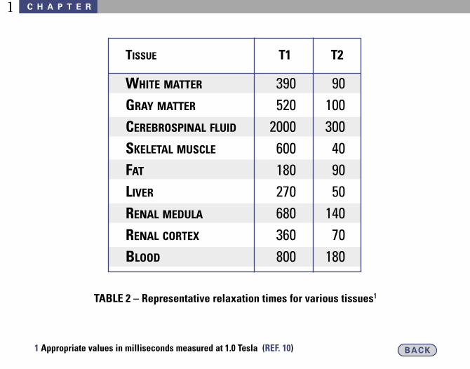
TABLE 2 – Representative relaxation times for various tissues1

C H A P T E R1

BACK1 Appropriate values in milliseconds measured at 1.0 Tesla (REF. 10)

TISSUE T1 T2

WHITE MATTER 390 90GRAY MATTER 520 100CEREBROSPINAL FLUID 2000 300SKELETAL MUSCLE 600 40FAT 180 90LIVER 270 50RENAL MEDULA 680 140RENAL CORTEX 360 70BLOOD 800 180

For a tissue like the white matter of thebrain containing a great amount of highmolecular weight lipids (myelin), waterspends less time in a bound state than itmight otherwise—simply because oil andwater do not mix.

The strength of the B0 field also influencesrelaxation times. This is due to the fact thatthe efficiency of relaxation is related to theratio of the tumbling rate to the reciprocalof the Larmor frequency. In general, T1relaxation times are shorter at lower fieldstrengths. The presence of paramagneticspecies such as iron and paramagnetic contrastagents (e.g. Gd + 3 DTPA) will shortenrelaxation times. Their ef fect is firstobserved on T1 and then with increasingparamagnetic concentrations, on T2 as well.For more information on basic spin physicsof relaxation, the reader is directed to(REFS. 1–4) in the Bibliography.

THE EFFECT OF MAGNETIC FIELD GRADIENTS

In a broad sense, a magnetic field gradientsimply refers to the spatial variation of thestrength of the B0 field. This was encounteredpreviously when discussing the dephasingeffects of B0 inhomogeneity, which may beviewed as an irregular spatial variation of B0.For the purposes of imaging however, fieldgradients like those illustrated in (FIG. 13)are needed. The slope of the gradient, itsdirection (i.e. along what axis), and timingneed to be controlled. Furthermore, formost applications, the B0 field must becaused to vary in a linear fashion with distance.Note that a gradient does not change thedirection of B0 but rather it changes thespatial variation of the amplitude of theB0 field.

C H A P T E R 1

CONTINUED

FIGURE 13 – The object at the top of the figure contains two small waterfilled cylinders.(A) In the absence of a gradient, the B0 field is the same at all points in the object as

depicted by the set of vectors. Application of an RF pulse to the object yields a FlD con-sisting of a single frequency. (B) Here, a gradient of the B0 field is imposed along thex-axis of the object. The spins in the two cylinders are exposed to different B0 fieldsand thus possess different Larmor frequencies. An RF pulse now gives an FID which

is an interference pattern of the two frequencies.

C H A P T E R1

BACK

zy

x

Time Time

G = 0 G ≠ 0x x

Suppose that there exists a linear gradientalong one spatial axis. Since

[1] γB0 = F

the resonance (Larmor) frequencies of protonswill vary according to their positions alongthe gradient axis. This is key to the under-standing of image formation. Since we canmeasure frequencies and we know the imposedspatial variation of B0, the positions of res-onating protons can be determined fromtheir frequencies.

In summary, a magnetic field gradient caus-es transverse magnetization to precess at afrequency which is proportional to positionalong the gradient axis as follows:

[5] F = γ (B0 + r Gr)

Where r is position along the axis of thegradient Gr. The presence of a gradient hasno significant effect on longitudinal magne-tization.

Let us now consider the fate of transversemagnetization when a gradient is switchedon for a short period of time and thenswitched off (FIG. 14). It may seem odd atfirst, but transverse magnetization can“remember” the effect of gradients whichwere present at an earlier time. FollowingRF excitation and before imposition of thegradient, transverse magnetization arisingfrom three different positions along thegradient axis, are all precessing together(in phase) at the same frequency. When thegradient is turned on, the vectors rotate atdifferent rates (frequencies) according toposition. When the gradient is turned off,all of the precessional frequencies are againthe same, but the vectors representing trans-verse magnetization are no longer in phase.Continued precession, all at the samefrequency, will not change the angles (relativephases) between the three vectors. Theaction of the past gradient pulse is thusremembered as “phase memory” (REF. 5).

C H A P T E R 1

CONTINUED

FIGURE 14 – Phase memory. Spins at three distinct locations (A,B,C) along a gradientaxis is shown. A 90° RF pulse generates transverse magnetization from all three sites.

In the absence of a gradient, vectors A,B,C precess in phase. When the gradient isswitched on, the spins at locations A,B and C are exposed to different B0 fields, whichin turn give rise to different precessional frequencies for the three locations. While thegradient remains on, the relative phase angles, e.g. between vectors A and B or B and C,become larger and larger. However, when the gradient is switched off the precessionalrates for A, B, and C become equal again. Continued precession does not alter the

phase (angular) relationships between the three vectors.

C H A P T E R1

BACK

90˚RF

time

time

turn ongradient

turn offgradient

wait

wait

timeA, B, C

A

A

A

A

A, B, C

BB

B

BC

C

CC

FOURIER TRANSFORMATION

We have seen that the basis for image formationis a positionally dependent frequency responseof transverse magnetization. Thus, an imageis a graph of amplitude versus frequency(FIG. 15). There remains a problem, however.The signals that are received, like the FID in(FIG. 8) or the echo in (FIG. 10) are in theform of amplitude versus time, rather thanamplitude versus frequency, as needed foran image. At first this may seem to be a trivialproblem. Looking at the FID in (FIG. 8), thefrequency of the signal is easily determinedas the reciprocal of the time interval betweentwo adjacent peaks. What makes the problemless than trivial is that signals are receivedfrom all positions at the same time. Theresultant signal is the superimposition (or sum)of a multitude of frequency components,each with distinct amplitudes and relativephases. Thus, it is an interference patterncomposed of all these components. A procedureis needed which can determine what set offrequencies, amplitudes and phases wouldgive rise to the observed interference pattern.

Such a procedure would be called a trans-formation from the time domain to thefrequency domain.

Most MR imaging and NMR spectroscopymakes use of the Fourier transform (FT),named after J.B.J. Fourier (1768-1830) whodeveloped the mathematical theory. In 1960,researchers at IBM devised a new algorithmfor calculating the Fourier transform ofarbitrarily complex digitized waveforms.The new algorithm (the Fast Fourier transformor FFT) greatly reduced the number of arith-metic operations necessary to calculate Fouriertransforms. Although the required numberof operations is still quite large, fast computerscan accomplish an FFT in a fraction of asecond. (REF. 17)

A sinusoidal waveform (a sine wave) is com-pletely defined by specifying three quantities:the amplitude, the period (or its reciprocalfrequency) and the phase. The phase of asinusoid describes what point in the wavecycle the sinusoid displays a given time versusa reference sinusoid of the same frequency.

C H A P T E R 1

CONTINUED

FIGURE 15 – (A) The Fourier transform is a mathematical process which mediates theinterconversion of time (units of sec.) and frequency (units of 1/sec. = Hz) descriptionsof waveforms. If two adjacent peaks in FID “A” are found to be separated by 0.01 see,the FT will yield a peak at 1/0.01 sec., = 100 Hz. (B) The power of the FT is its ability tosort out arbitrarily complex time domain waveforms into their individual frequency

components The time domain signal here is an interference pattern which arose due toimposition of a gradient across the object in FIGURE 13. The FT shows the two compo-nent frequencies. Since the gradient causes variation of frequency with distance, thefrequency domain here represents a one-dimensional projection image of the object.

C H A P T E R1

BACK

(A)

(B)

Time Frequency

This is the same as the description of therelationship between the three vectors inthe last section after turning off the gradient.Fourier transformation conserves all threepieces of information. In clinical MR imaging,however, the phase information is usuallydiscarded at the final stage of reconstruction.

Frequency is the reciprocal of time, andtime is the reciprocal of frequency; the FTof the time domain is the frequency domain,and vice versa. The information content inthe two domains is identical, but the formatis different.

The necessity of examining information in onedomain instead of the other actually arisesfrom the constraints of human perception.(For an example, see the Reconstruction sectionunder MR Imaging Techniques.) We are capableof something like a mental FT when we listento a chord of music. The sound arrives at ourears as an interference pattern of the notesof the chord; however, we can still discernindividual notes played together to yieldthat chord (REFS. 4, 18). By contrast, the eyeis not capable of extracting individual wave-lengths of, say, white light. This decomposition,however, can be achieved by means of a prismwhich serves as a Fourier analyzer.

C H A P T E R 1

CONTINUED

C H A P T E R 2

CHAPTER 2

PRINCIPLES AND TECHNIQUESIN MR IMAGING

CONTINUED

Beyond the nominal strength of the B0 field,the homogeneity of this field over the imagingvolume must be considered. B0 inhomogeneityof just a few parts per million (ppm) leadsto noticeable shading of MR images, whilegreater inhomogeneities give rise to spatialdistortions in the images.

Clearly, much of the advantage of high-fieldstrength can be lost without sufficienthomogeneity. B0 homogeneity is optimizedby a procedure known as “shimming”. Here,the magnet is fitted with a set of electromagneticcoils. By carefully adjusting the amount ofcurrent in each of these coils, the B0 fieldover the imaging volume is adjusted orshaped until acceptable homogeneity isachieved.

INSTRUMENTATION

From the preceding discussion, the equipmentnecessar y for MR imaging can largely beinferred. A typical MR imaging system blockdiagram is given in (FIG. 16).

The B0 FieldThe source of the static B0 magnetic field isa magnet large enough for a person to bepositioned in its homogeneous portion. Theproperty of prime importance is the strengthof B0. High magnetic field strengths aredesirable because, as discussed on pages 72-78, this parameter ultimately limits thestrength of the MR signals to be received.High magnetic field strengths require asuperconducting magnet such as that dia-gramed in (FIG. 17).

FIGURE 16 – Functional block diagram of an MR imaging system.

C H A P T E R2

BACK

OPERATING CONSOLE

MAGNET

CRT

Computer

Digitizer

Keyboard

Receiver

Transmitter

Gradient Amplifier

RF Coil

RF Coil

GradientCoils

FunctionButtons

TrackBall

DiskDrive

Multi-FormatCamera

Magnetic Tape Unit

FIGURE 17 – Cross-sectional view of superconducting magnet.

C H A P T E R 2

BACK

HELIUM

NITROGEN

MAGNETS ANDSHIM COILS

VACUUM

WARM BORE

OUTSIDE OFN2 VESSEL

Magnetic Field GradientsAs discussed earlier, gradients in the B0 fieldalong the three orthogonal spatial axes arefundamental to image production. Gradientsalong other oblique axes can be implementedwith combinations of the orthogonal gradients.

(FIG. 18) shows the basic scheme for obtaininga B0 gradient parallel to the direction of B0.Two coils of wire (a), and (b), are suppliedcurrent which generates magnetic fields,adding (a) or subtracting (b) from the mainB0 field. At any given point along the gradientaxis, the net magnetic field is equal to thesum of B0 plus the magnetic field contributionfrom coil (a) plus the contribution from coil(b). It is the coil which is closer to the positionof interest that has the greater effect on thenet magnetic field.

Note that at a point midway between thetwo coils, the magnetic fields generated bythe two gradient coils cancel each other,causing the net magnetic field to be equalto B0. The gradient coils are positioned suchthat this mid-point is at the center of the B0magnet, and is denoted as the isocenter.

The gradient coils on the other two orthogonalaxes are constructed differently, but they alsocause additions and subtractions to the B0field dependent upon position alone theseaxes. Additionally, the mid-points of no netgradient contributions are positioned tooccur at the magnet’s isocenter. Power issupplied to each of the gradient coils byindependent computer-controlled gradientamplifier.

What properties of the magnetic field gradientsimpact upon system performance and ultimatelyimage quality? There are several. As shown inthe next three sections, the maximum attainablegradient amplitude (or slope, which is thechange in magnetic field per unit distance,often cited in terms of Gauss/cm) limits theminimum slice thickness and the minimumfield-of-view (FOV) that can be used. Gradientlinearity refers to the uniformity of the slopealong the gradient axis; non-linearity yieldsimage distortions.

C H A P T E R2

CONTINUED

FIGURE 18 – The design of a gradient coil acting parallel to B0. The coil is divided intotwo sections (a and b) which are supplied DC current from the gradient amplifier forthis axis. Coil “a” produces a magnetic field Ba which adds to B0, while coil “b” pro-duces Bb subtracting from B0. The strength of Ba and Bb. decreases with increasing

distance from coils “a” and “b” respectively, while the strength of B0 is constant overthis region. At any point along this axis the net magnetic field (Bnet) is the sum of

B0, Ba, and Bb. This results in a linear variation of Bnet; Ba and Bb cancel at isocentergiving Bnet, = B0 at that position.

C H A P T E R 2

BACK

Current

Current

IsocenterIsocenterDistance

alongthe Axis

+ BaB0– BbB0 B0

Bb

Ba

B0 a

b

FromGradientAmplifier*

In practice, gradients are not powered at alltimes, but are switched on and then off again(pulsed) at certain times during a pulsesequence. This raises further concerns. Howfast a gradient can be powered from zero tofull amplitude is referred to as the “rise time,”which should be as short as possible.

But the act of switching gradients on andoff causes another problem. It induces theformation of electronic currents, so-called“eddy currents” in the metallic structures ofthe magnet. These eddy currents generatemagnetic fields of their own, which dissipateat differing rates. Clearly, eddy currents areundesirable and can have deleterious effectson image quality.

One solution to this problem is to drive thegradient coils not with the desired pulseshape, but rather with an empirically deter-mined pulse shape which cancels out eddycurrent contributions and yields the desiredgradient in the magnet.

A potentially more powerful approach is the useof self-shielded gradient coils. These coils areconstructed such that the magnetic fieldsgenerated by them are confined to the interiorof the coils thus preventing the formation ofeddy currents in the remainder of the magnet.

The B1 FieldThe basic RF architecture for generation ofRF pulses constituting the B1 field is diagramedin (FIG. 19). An extremely precise and stablesource of RF at low power levels is a digitalfrequency synthesizer set to yield RF at theproton Larmor frequency (F0) in the absenceof gradient contributions. As discussed underslice selective excitation (Last Section), it isuseful to be able to make small changes (∆F0)to the value of F0; waveform modulation andpulse control are also essential. An RF poweramplifier then varies the RF power to thatrequired for imaging. All of these stages arecontrolled by a computer, which is alsoresponsible for pulse sequence execution. Thefinal RF energy is sent to the RF coil in themagnet which acts as a broadcasting antenna.

C H A P T E R2

CONTINUED

FIGURE 19 – Functional block diagramof the RF transmitter section of an MRinstrument. A digital frequency syn-thesizer with a thermostated quartzcrystal reference produces lowamplitude RF of frequency F0 whichis the Larmor frequency at B0. Sliceselective excitation requires the abilityto make small frequency changes toF0, which is accomplished by additionor subtraction of an “offset” frequency(∆F0). Waveform modulation serves tocontrol the profile of the excited slice,and pulse control determines whenRF is allowed to pass to the final RFpower amplifier.

C H A P T E R 2

BACK

SOURCE OFRF FREQUENCY = F0

FREQUENCY SYTHESIZER

SMALL FREQUENCYCHANGES BY ADDITION

OR SUBTRACTION OF ∆F

PULSE CONTROL ANDAMPLITUDE MODULATIONWITH “SINC” WAVEFORM

RF POWER AMPLIFIER

RF COIL INSIDE MAGNET

F0 ± ∆F

PULSES OF F0 OF ∆F

F0

PULSES OF F0 OF ∆F

COMPUTER

For most applications, it is desirable for theRF coil to distribute the RF energy uniformlythroughout the imaging volume. The degreeto which this is achieved depends primarilyon the design of the RF coil. Critical Performancespecifications include the maximum amountof power that the RF power amplifier iscapable of producing.

Remember, the flip angle is proportional toboth the duration and the amplitude of theRF pulse. Furthermore, the linearity of thisamplifier is critical. A linear amplifier is onein which a change in the amplitude of theinput signal leads to a directly proportionalchange in the amplitude of the output signal.RF amplifier non-linearities yield flip angleerrors as well as distortion of the shape ofan excited slice.

The ReceiverThe task of the MR receiver can be appreciatedwhen it is realized that the signal resultingfrom nuclear transverse magnetization is approx-imately one billionth that of the transmittedRF power. A simplified design of an MR receiveris given in (FIG. 20).

Transverse magnetization induces an ACcurrent in the RF coil used for reception;this coil may or may not be the same RF coilused for production of the B1 field. The RFsignal, which is approximately at the Larmorfrequency for the B0 field is amplified by afactor of 104 to 105 by the RF preamplifier.It is technically quite inconvenient to workat these high frequencies. The ultimate functionof the receiver is to correctly represent theamplitude, periodicity and the phase of theincoming MR signal in computer memory.For this purpose, it is only necessary to measurethe MR signal relative to a known standard.

The standard used is a RF source called thelocal oscillator, which in fact is often a portionof the RF signal from the frequency synthesizerused for transmission. The mixer then yieldsa signal which is the difference between theRF transmitted and the signal received. Thisdifference signal is in the range of audiofrequencies (AF). It is this range of frequen-cies which are of concern for the receiverbandwidth.

C H A P T E R2

CONTINUED

FIGURE 20 – Block diagram of an MRreceiver. Transverse magnetizationinduces an AC current in the RF coilwhich is amplified. This signal ismixed with a reference RF signal fromthe “local oscillator;” this oscillatormay actually be the frequency synthesizerused for RF transmission in FIGURE 19(not true for off-center FOV). The lowfrequency (AF) signal which is thedifference between the incoming RFand the local oscillator RF is thenamplified, digitized and stored incomputer memory.

C H A P T E R 2

BACK

RF COIL

RF PREAMPLIFIER

MIXERS AND FILTERS

AF AMPLIFIERAND FILTERS

ANALOG-TO-DIGITALCOVERTER (ADC)

RF

AF

RF

AF

COMPUTER

COMPUTER MEMORY

BINARY DATA

The AF signal is amplified by a factor of 10to 1,000 by an AF amplifier. The signal is nextdirected to an analog- to-digital converterwhich converts the AF signal into a series ofbinary numbers. These numbers are thenstored in computer memory for later manip-ulation (signal averaging and Fouriertransformation).

The most critical design feature of thereceiver is the combination of the quality ofthe RF coil and RF preamplifier. These twocomponents predominantly determine theamount of system noise added to the MRsignal. Of somewhat lesser importance forimaging is the precision of the ADC; 12-bitresolution is usually sufficient for imaging.

The Computer SystemA modern MR instrument imager has severalcomputers linked by a communications network.For example, the current Signa® system hasfour computers: a host computer, an arrayprocessor, and two specialized computerswhich are the status control module (SCM)and the pulse control module (PCM). It isnot necessary to have this particular parti-

tioning of computing power. Therefore,the features of a MR computer system asa whole will be discussed here.

Core memory is directly accessed by the centralprocessing unit(s) (CPU). This memory mustbe sufficiently large to contain all of theinstructions and waveforms for one pulsesequence, an entire raw image data set, anda certain amount of operating software. Theremaining software and data requirementscan be met with disk memory.

An array processor is needed in order toaccomplish image reconstruction quickly.This implies that the array processor requiresdirect access to at least enough memory tocarry-out reconstruction of an entire image,otherwise disk access operation becomesrate-limiting. Since pulse sequences mustexecute in “real time,, the computer systemmust give top priority to pulse sequenceinstruction execution. The receiver ADCmust have buffered memory access to ensurethat incoming data can be stored quicklyenough that data are not missed or lost.

C H A P T E R2

CONTINUED

Long-term data storage (archiving) isgenerally relegated to streaming tape.

The computer system described here is a mini-mal configuration. In actual practice, morepowerful systems are employed in order toease prescriptions and routine operations.

In the following discussion of the imageacquisition process, we will concentrate onthe most commonly implemented clinicaltechnique, i.e. two-dimensional Fourier trans-form imaging utilizing spin-warp encodedspin echoes. (REFS. 5–8, 23).

SLICE SELECTIVE EXCITATION

In 2D-imaging schemes, signal response in thethird spatial dimension needs to be restricted.This is accomplished by selectively exciting(converting longitudinal magnetization intotransverse magnetization) only spins in a welldefined slice of tissue within the imaging volume.This is accomplished by imposing a gradienton an axis perpendicular to the chosen sliceplane, which causes a linear variation ofpotential resonance frequencies along that

axis (FIG. 21). Input of RF energy consisting ofa narrow range of frequencies (RF bandwidthdenoted as ∆F) excites only those spins alongthe slice selection axis whose resonance frequen-cies, as dictated by the gradient, correspondto the frequencies present in the RF. Afterthe RF pulse, the slice selection gradient isturned off, and signals emanating from thechosen slice can be detected.

Quantitatively, the thickness of the excitedslice (dsl) in cm is related to the gradientamplitude Gslice and RF bandwidth ∆F as follows:

[6] ∆F = γH * Gsl * dsl

For example, suppose that without any gradientall protons resonate at 64.000 MHz and that theRF covers the range 64.001 MHz to 63.999 MHz.The RF bandwidth (∆F) is 0.002 MHz 2000 Hz.If a gradient amplitude of 0.5 Gauss/cm isimposed and the RF pulse is issued, the thick-ness of the excited slice is:

2000 Hz————————————— = 0.94 cm4257 Hz/Gauss x 0.5 Gauss/cm

C H A P T E R 2

CONTINUED

FIGURE 21 – Slice selective excitation is accomplished by the use of narrow bandwidth(∆F) RF in combination with a gradient along the slice axis. A and B show two possiblestrategies for variation of slice thickness. In A the gradient amplitude is varied, while inB the gradient amplitude is constant but ∆F is changed. In C, different slice locations are

chosen by changing the RF center frequency (F0).

C H A P T E R2

BACK

∆Fa ∆Fb

∆F0

∆F0 (b)

∆F0 (a)

a∆F

∆F

dsl (b)

dsl (a)

∆FF0

Ga

Gb

b

F0

dsl (b)

dsl (a)

G

GA B

C

Position along the slice axis

Reso

nanc

e Fr

eque

ncy

Reso

nanc

e Fr

eque

ncy

Reso

nanc

e Fr

eque

ncy

If a thinner slice is desired, two options becomeevident from Equation [6]: either (a) the RFbandwidth must be decreased or (b) the gradientamplitude must be increased.

Let’s assume a single slice has been excited.But which slice? And at which location alongthe gradient axis? As noted in the previoussection, the gradient coils are constructedsuch that the zero point of the gradient is amagnetic center (the isocenter) of the magnet.This means that for any of the three gradientsat any amplitude, B0 at isocenter is unchanged.Along a given axis, the gradient causes a linearincrease of B0 on one side of isocenter, anda linear decrease of B0 with increasing distancefrom the other side of isocenter.

Now, the location of the excited slice can bedetermined. Since the center frequency of theRF (F0) was equal to the resonance frequencyof protons in the absence of a gradient, andsince at isocenter there is no change to B0when a gradient is on, the slice excitedabove was located at isocenter + 0.47 cm.

This, however, raises yet another question.How can one selectively excite an off-isocenterslice? Again there are two options: (a) changethe position of the zero point of the sliceselection gradient with respect to isocenter,or (b) change the center frequency of theRF to correspond to a resonance frequencywhich is either higher or lower than the protonresonance frequency without gradients. Practicalconsiderations force the choice of the latteroption. This method of offsetting a slice fromisocenter is also easy to examine quantitatively.If the same slice thickness, gradient amplitudeand bandwidth (∆F) as in the above exampleare employed, then the needed change for theRF center frequency (∆F0) is expressed by:

OFFSET * F[7] ∆F0 = —————

dsl

where offset is the distance from isocenterfor the center of the desired slice.

C H A P T E R 2

CONTINUED

For example, if the desired slice location is+3.76 cm from iso-center then the center RFfrequency is changed by:

3.76 cm x 2000 Hz∆F0 = ————————— = + 8000 Hz0.94 cm

Now the RF covers the range 64.009 MHzto 64.007 MHz.

There is one more issue in the slice selectionprocess that merits discussion.

If one could examine the excited slice and itsprofile edge-on, how would it appear? Onemight hope that the slice profile would berectangular; however, without special precautionsthis would not be the case. It is necessary toinsure that the flip angle is uniform acrossthe slice If RF at frequency = F0 is just switchedon for some period of time and then switchedoff, the flip angle will not be the same at alldepths in the slice (FIG. 22). The nonuniformityof flip angle across the slice is a consequenceof the variation in RF amplitude at differentfrequencies (depths in the slice). We now seethat earlier statements concerning RF covering

a range of frequencies bore a rather stringentimplied assumption: there is an equal amountof RF power input for all frequencies within F,and no power outside of this range.

The FT can point to the solution of this problem.Note that in (FIG. 22A), the rectangular pulseof RF is a description of amplitude versus time,while its corresponding plot of RF power distri-bution is amplitude versus frequency. This shouldsound familiar. Indeed the FT of a rectangularpulse envelope is this curve defined by thefunction sin x/x called a “sinc” waveform. Dueto the aforementioned reciprocity betweenthe time and frequency domains, the solutionsuggested is as depicted in (FIG. 22B). If a rectan-gular frequency domain profile is desired, thenthe FT of a rectangle, namely the sinc shapeis the needed time domain description of theRF pulse. In practice then, the RF pulse offrequency = F0 is multiplied by the sinc wave-form before sending the pulse to the RF coilin the magnet. We have seen how to confineexcitation to a single slice in the imagingvolume.

C H A P T E R2

CONTINUED

FIGURE 22 – (A) Although the reasons are notintuitively obvious, a short burst or pulse of singlefrequency RF does not result in deposition of RFpower at just one frequency. Instead, the RFpower is spread over a range of frequenciescentered at F0. If such a pulse of RF were usedfor slice selection, the variation of RF poweracross the resonance frequencies containedin the slice would yield variations in flip angleacross the slice. (B) This situation is avoidedby using a “sinc” shaped RF pulse to give arectangular RF power spectrum. (C) Sinc pulsesare incorporated into a slice selective spin echosequence. Note the standard schematic represen-tation of gradient action. The height of a gradientpulse represents the amplitude or slope of thegradient, and the width its duration. Whetherthe gradient causes increasing or decreasingB0 when moving in a positive direction alongthe gradient axis is indicated by a pulse up ordown. The small negative-going lobe of Gsliceaccounts for dephasing which occurs duringthe slice selective 90° pulse.

C H A P T E R 2

BACK

A)

B)

C)

RF of Frequency F0

F0

Time

Amplitude AmplitudeFT

FT

Time

Frequency

Frequency

ExcitationPowerSpectrum

F0

F0

0

RF

Gslice

Receiver

Echo

90˚180˚

TE/2 TE/2

∆F=1/

F +1/0τ

τ τ

τ

In fact, since spin-echoes are to be used, twoselective RF pulses, a 90° pulse and a 180° pulse,are employed to obtain a slice selectivespin-echo.

FREQUENCY ENCODING

The next task is encoding the image informationwithin the excited slice. The image informationsought is actually the amplitude of the MRsignal arising from the various locations in theslice. Two distinct processes are used for encod-ing the two dimensions, called frequencyencoding and phase encoding. Frequency encod-ing will be discussed first.

The general strategy for gaining spatial infor-mation along one axis of the image plane isshown schematically in (FIG. 23A). For reasonsof sensitivity, it is desirable to have the receiveron only while the echo is present, and to havethe center of the echo form in the middle ofthis “acquisition window”. This action, in com-bination with slice selection, would not yieldinformation about distribution of spins withinthe slice, because all positions would resonateat the same frequency. Imposition of a gradient

along one of the two principal axes of the planeduring the period when the receiver is on,causes the signal received to be an interferencepattern arising from the various precessionalfrequencies of the spins along the gradientaxis, hence the name frequency encoding Thisgradient is sometimes referred to as the “read”,“read-out”, or “frequency-encoding” gradient.The FT of the signal acquired in the presenceof the read gradient is an image of the pro-jection of the slice onto the read gradientaxis. (FIG. 13) & (FIG. 15)

If only the read gradient pulse were playedon this axis, severe dephasing of the echoand concomitant loss of signal intensity wouldbe anticipated. In order to avoid this, anothergradient pulse, termed a “dephaser”, is alsoimplemented along the frequency encodingaxis. Note that the area of the dephaser gradientpulse is one half that of the read gradient.The dephaser changes the phase of transversemagnetization by amounts which are propor-tional to position along this axis (FIG. 23B).

C H A P T E R2

CONTINUED

FIGURE 23 – Frequency encoding. (A) Thefrequency encoding gradient is played alongone of the two principal axes with the selectedslice. The read gradient pulse causes the fre-quencies contained within the spin echo tobe proportional to the positions of respondingspins along the axis of the frequency encodinggradient. In order to avoid severe dephasingof the echo due to the read gradient, a “dephas-er” of pulse is used. (b) Instead of representingphases by the direction of vectors in a circlein the transverse plane, a useful conventionis a phase plot where the circle is representedon an axis running from + 180° to -180°. Thedephaser causes a positionally dependentphase change as shown for three positions(FIGURE 14). The 180° pulse reverses thesephases, and the first half of the read gradientcauses rephasing; all positions are in phaseat echo time.

C H A P T E R 2

BACK

A)

B)

RF

Gslice

Receiver

Echo

Gfrequency encode

Phase

Dephaser Read

90˚180˚

TE/2 TE/2

180˚ TE

The 180° pulse inverts this phase distribution,just as it did in the discussion of spin-echoformation. The action of the first half of thegradient over the acquisition window now actsto compensate the phase shift caused by thefirst gradient pulse on this axis. In this manner,complete rephasing occurs at time TE, i.e. inthe center of the acquisition window.

The details of the frequency encoding pro-cedure dictate the field of view along thisaxis: (FOVf).

[8] γGf • FOVf = BW

Where Gf is the amplitude of the frequency-encoding gradient, and BW is the receiverbandwidth. Note that Equation [8] is directlyderived from the Larmor equation. The receiverbandwidth should not be confused with theRF bandwidth discussed in the previous section,although the relationships between the variousquantities are closely analogous in the twosituations.

In order to gain an understanding of receiverbandwidth and its role in determining the FOV,

it is necessary to review the action of the MRreceiver, and examine the details of signaldigitization.

Within the receiver, the incoming RF signalis converted to a much lower (AF) frequencywhich is the difference between the RF trans-mitted and that received. This differencesignal is digitized by sampling the voltage ofthe signal at discrete intervals and then repre-senting these voltages as digital numbers tobe used by the computer (FIG. 24). Samplingtheory dictates that in order to gain a correctdigital representation of the frequency of asinusoidal waveform, it is necessary to samplethe waveform at least twice per cycle.

Thus, it is the rate at which the signal is sampledwhich determines the maximum interpretablefrequency in the signal. This maximum frequencyis called the Nyquıst frequency. Frequenciespresent in the signal which are higher than theNyquist frequency will be misrepresented indigital form, and will appear to be contributionswhich are lower than the Nyquist frequency.This is the cause of “wrap-around” artifacts.

C H A P T E R2

CONTINUED

FIGURE 24 – A sine wave (solid line) is “sampled” at the times of the open circles andthe amplitudes at those times are digitized for computer storage. However, if the sinewave is not sampled at least twice per cycle (closed circles), the computer representation

of the sine wave gives an erroneous impression of the wave’s frequency.

C H A P T E R 2

BACK

Amplitude

Time

The effective range of frequencies that canbe properly detected (receiver bandwidth) iscontrolled by the digital sampling rate, whichin turn is determined by the number of pointson the signal to be digitized and the lengthof time that the receiver is on. Therefore:

[9] BW = Nf / T

Where Nf is the number of complex points*sampled, and T is the sampling time.

As an example, let us examine the defaultvalues implemented on the Signa system. Allavailable matrix sizes use 256 complex points inthe frequency encoding dimension, and acqui-sition window duration 8 msec. The receiverbandwidth is:

256/.008 = 32.000 Hz = ±16 kHz)*BW = ———————————————2 x 0.008 sec

The FOVf is adjusted through variation ofthe amplitude of the read gradient (G f ).If Gf= 05 Gauss/cm, then:

FOVf = ±1600 Hz / 4257 Hz/Gauss x 0.5 Gauss/cm = 7.51 cm

Clearly, if Gf is increased, then FOVf will decrease.

Intuitively, we see that the spatial resolutionalong this axis must be related to the distancecovered in this image dimension (FOVf) andthe number of data points describing thisdimension. From Equations [8] and [9], thepixel size along the frequency encoding axis(FOVf/Nf) may be derived, giving:

[10] FOVf / Nf = 1 / (γGf T )†

The factor of two in the definition of pixel sizeresults from the fact that half of the pointsafter FT only give additional phase information.Equation [10] shows that there are two ways toincrease the resolution: (a) increase Gf, causingFOVf to decrease, or (b) increase both Nf andT by the same factor which leaves BW andFOVf unchanged.

* A complex point of measured signal consists of two numbers which describe the vector components along each of the two principle axes.

† Rather than sampling frequencies between 0 and 32 kHz, quadrature phase detection allows examinationof frequencies from –16 kHz to +16 kHz relative tothe local oscillator frequency.

C H A P T E R2

CONTINUED

PHASE ENCODING

The process of frequency encoding yields,after FT, a projection of the image plane ontothe read axis. As stated in the section onFourier transformation, three pieces of infor-mation are conserved: frequency, amplitudeand phase. In the projection, variations infrequency denote position along the read axis.And variations in amplitude yield informationon the total signal intensity contained in thecolumn represented by each point along theprojection. Note, however, that variation inphase has not thus far been used to provideimage information. In order to produce atwo-dimensional image of the slice, one couldcause a systematic variation in phase whichwould encode the spatial information alongthe one remaining principal axis of theimage plane.

(FIG. 25) shows a complete 2D-imaging pulsesequence. The only addition to the pulsesequence relative to that considered previouslyis a single gradient pulse on the third gradientaxis (phase encoding axis). Since this phaseencoding gradient is not on within the acqui-

sition window, it cannot affect the detectedfrequencies. However, as we have seen previously,the phase change of transverse magnetizationdue to this gradient pulse will be preservedin the form of phase memory. The inducedphase change is proportional to the amplitudeand duration of the gradient times the positionof spins along that axis.

Implementation of phase encoding is accom-plished as follows. The complete pulse sequenceis played out many times (typically 128 or 256times) and the resulting signals are storedseparately. The only variation from one acqui-sition to the next is the amplitude the phaseencoding gradient which is changed in a step-vfashion. Separate Fourier transformation ofeach of the data sets (“views”) yields a setprojections onto the read axis These projectionsare expectedly identical to one another withrespect to frequency but not with respect to phase.

If this were x-ray CT, collecting a set of viewswhich we all projections onto the same axiswould be a pointless exercise.

C H A P T E R 2

CONTINUED

FIGURE 25 – The final dimension of spatial information is obtained by phase encoding.Each view is obtained using a different amplitude for the phase encoding gradient

lobe. The action of this gradient is still “remembered” at echo time as phase memory.

C H A P T E R2

BACK

TE/2 TE/2

90˚180˚

RF

Gslice

Receiver

Gfrequency encode

Gphase encode

However, if one were to choose any givenposition of one of these MR views, and thenfollow the phase at that point progressingfrom view view to view, variation would be noted.This variation is another interference pattern.Following a different point from view to viewreveals a different interference pattern. Sincethe only change in the pulse sequence fromview to view is the amplitude of the phaseencoding gradient, the noted interferencepatterns reflect the sum of phase changesalong the phase encoding axis. Another setof FTs is certainly indicated.

A data set consisting of the first point fromevery projection is constructed and subjectedto FT (FIG. 26). Another data set is assembledfrom the second point on every projection,Fourier transformed and stored separately.Then, all of the third points are used, etc.The result is a 3D plot of signal amplitudeversus location on the frequency and phaseencoding axis. If amplitudes are convertedto gray scale, the result is the image of the slice.

Finally, let us consider phase encoding quanti-tatively. A data set formed by taking the samedata point from each of a set of views, represents

a discrete digital sampling of an interferencepattern. Therefore, the same sampling theoryprinciples which were applied in the frequencyencoding dimension, also need to be consideredfor phase encoding. Specifically, the requirementfor sampling at least twice per cycle must bemet. To phase encode one cycle requires a 360°phase change, necessitating at least one samplefor every 180° phase change. This means thatthe two edges of the FOV in the phase encodingdimension correspond to those positions alongthe phase encoding gradient axis when eachincremental change in the gradient amplitudecauses a 180° phase change. At positions betweenthese two points, the phase changes by lessthan 180 ° per view. In analogy to Equation[8] we can write:

[11] γGP * FOVP * TP = NP * π

where Np is the number of phase encodings(views), Tp is the duration of the phase encodinggradient pulse, FOVp is the FOV in the phaseencoding dimension and Gp is the maximumamplitude of the phase encoding gradient.

C H A P T E R 2

CONTINUED

FIGURE 26 – Schematic representation of imageformation by 2D-FT. (A) This represents a slicethrough an object containing 3 vials of water(labeled 1, 2 and 3). The projection onto thefrequency encoding axis is shown behind the slice.(B) Collection of MR data from the slice yieldsa set of spin echoes (views). Note that each echois produced from the entire slice. (C) Fourier trans-formation of all of the views yields a set of pro-jections of the slice onto the frequency encodingaxis. The oscillations underneath the envelopeof each projection represent one-half of the phaseinformation. (D) A new data set is assembled fromthe columns in C (added views have been filledin). Some of the rows of the new data set containno signal because these rows correspond to posi-tions along the frequency encoding axis wherethere is no water. Two of the depicted rows docontain signal. The lower of these two rows is asignal containing a single frequency, while theupper row is an interference pattern of two sinu-soids. (E) FT of all of the rows in D produces theimage. The image needs to be rotated and flippedin order to correspond to the slice depicted in A.Note that the data would have a more complexappearance if the vials of water were larger thanone pixel each; resonances from one portion ofa vial would interfere with resonances fromother portions.

C H A P T E R2

BACK

A)

collectMR data

phaseencoding

frequencyencoding

frequencyview #

view #

time

FT

FT

FT

FT

FT

FT

FT

FT

FT

FT

FT

FT

FT

FT

C)

D)

B)

E)

1

2 3

2 1

3

The spatial resolution can be expressed as thepixel size which, in phase encoding direction,is equal to the ratio FOVp/Np for which weobtain from Equation [11].

[12] FOVP / NP = π / (γGPT )

Hence, we can lower pixel size by increasingthe amplitude of the phase encoding gradient(in analogy to the frequency-encoding gradientwhich controls the pixel size in the read directionof the image). Alternatively, however, we canincrease the duration of the phase encodinggradient.

RECONSTRUCTION

Reconstruction is a term brought to MR fromCT, where it refers to projection reconstructionwhich is the mathematical process used totransform raw data into a CT image. As wehave seen, the two-dimensional Fourier trans-form method used in MR is a very differentkind of process than projection reconstruction.

In MR, the word “reconstruction” has a moregeneral connotation, and denotes all of the

computer processing interposed between rawdata and image. The 2D-FFT is central to thisprocessing, but it also includes baseline corrections,mathematical weighting of the raw data forartifact reduction and other purposes, post-2D-FFT data filtering for edge enhancementor smoothing, magnitude calculation, correctionsfor gradient imperfections, scaling for imageprocessing, and image reorientation (rotating,and flipping) for a standardized presentationformat.

Let us follow the processing from raw datato image for an MR image. (FIG. 27A) showsthe raw data for the image in (FIG. 27C), while(FIG. 27B) shows an intermediate step afterthe first dimension of FT, i.e. all of the viewshave been transformed in frequency-encodingdirection. In all three figures the phase infor-mation has been discarded; the brightness ateach point represents signal amplitude. Highsignal is represented as white (note that thisis the opposite of the convention used inCT, where white means high attenuation).

C H A P T E R 2

CONTINUED

FIGURE 27A – Reconstruction. (A) This is the not-so-mysterious k-space data or raw data.Each view is a spin echo; the middle views have the greatest amplitude because they

were obtained with the weakest amplitudes of the phase encoding gradient.

C H A P T E R2

BACK

C H A P T E R 2

BACK

FIGURE 27B – Reconstruction. (B) The FT of any one of the views gives a projectiononto the frequency encoding axis. View No. 128 is displayed on the right.

C H A P T E R2

BACK

FIGURE 27C – Reconstruction. (C) The second dimension of FTs yields the image.

MULTISLICE ACQUISITION

Thus far the acquisition of image data for onlya single slice has been considered. The questionnaturally arises: How much time is neededto acquire these data? The answer is:

[13] Total Acquisition Time = Number of viewsx Number of excitations per view x TR

The number of views collected for an image isdefined by the selected matrix size. Typicalmatrix sizes are: 256 x 128, 256 x 192, and256 x 256.

The second number of each pair representsthe number of views. Clearly, as discussed inmore detail below, if one were to collect allthe image data from one slice, and then repeatthe entire acquisition for the same slice, thetwo data sets could be added together in orderto gain SNR. This is the process which is alludedto by the term “Number of excitations per view,”also abbreviated as NEX. A typical set of imagingparameters might be: TR = 1000 ms, TE = 25 ms,NEX = 2, Matrix = 256 x 128.

The total acquisition time for one image(slice) would be 128 views x 2 excitations perview x 1000 ms per excitation = 256,000 ms =256 sec = 4 min 16 sec

Does this mean that using this protocol wouldrequire 8 min 32 sec to acquire data for twoslices, and 12 min 48 sec for three images?This would be quite uneconomical since TEis much shorter than TR, implying that almostall of the duration of TR is “dead time” waitingfor T1 processes to restore longitudinal magne-tization in the excited slice. During this deadtime, we may be exciting and detecting adifferent slice parallel to the first slice. In fact,as illustrated in (FIG. 28), excitation/detectionmay be carried out in many parallel slices duringeach TR interval. There is easily enough timein the above example to collect data frommore than 20 different slices during the 1000 msTR interval. Thus, image data from at least20 different slices can be collected in the same4 min 16 sec calculated above for one slice.

C H A P T E R 2

CONTINUED

FIGURE 28 – Interleaved multislice acquisition. Since TR is usually longer than thetime required for excitation and detection in a slice, the remaining time within

each TR interval may be used for excitation/detection in other slices.

C H A P T E R2

BACK

Echo1

Echo2

Echo1

Echo2

Echo1

Echo2Receiver

RF

Slice #1 Slice #2 Slice #3

90º 90º 90º180º180º 180º180º 180º180º

TE TE TE TE TE TETR

CONTRAST

The intensity or brightness at any given positionin an MR image reflects the amplitude of theMR signal arising from that position, whichin turn is proportional to the concentrationof mobile protons (proton density, abbr. N(H))in that region. If imaging parameters are selectedwhich cause image intensity to reflect onlyvariations in N(H) across the image, the imageis termed a proton density image. An exampleof this is shown in (FIG. 29). The image has arather “flat” appearance, i.e. the intensity doesnot vary much from structure to structure.The reason for this appearance is that N(H)does not vary greatly in different tissues.Therefore, it is desirable to seek other sourcesof contrast which vary more significantly fromtissue to tissue; the relaxation times T1 andT2 are good candidates for sources of contrast.In the following we will examine extremecases of contrast (REF. 12).

Suppose there were two adjacent tissues ofequal mobile proton density but possessingdifferent relaxation characteristics. Both tissueswould be subjected to a long train of spin-echo

sequences, just as in image data collection.The two important operator controlled acquisi-tion parameters involved are TR and TE.

CASE 1: TR is very long (TR >> T1) and TEis very short (TE << T2). Since TR is verylong, both tissues completely recover all oftheir longitudinal magnetization betweeneach spin-echo excitation/detection sequence,even though the two tissues possess differentT1 values. Therefore, differences in T1 valueswill not affect the amount of longitudinalmagnetization which is available for a subsequentspin-echo in the train. We have also assumedthat the two tissues possess different T2 values.Remembering that T2 relaxation describesthe rate of decay of signal in the transverseplane, a long TE would yield different amountsof signal from tissues possessing different T2s.However, in this case TE is very short so thesignal from neither tissue has time for muchdecay at all. Thus, neither differences in T1nor differences in T2 will effect signal intensity.These conditions yield a proton density image(FIG. 29). The two tissues will appear isointensedue to their equal N(H) values.

C H A P T E R 2

CONTINUED

FIGURE 29 – Proton density weighted images are obtained by using a long TR anda short TE (TR = 6000 ms, TE = 20 ms). Note the rather uniform intensity across the

various brain structures. On the graphs, two tissues with differing relaxationcharacteristics are indicated as a and b.

C H A P T E R2

BACK

Time

Time

TR

TE

a

b

a

b

MLONGITUDINAL

MTRANSVERSE

CASE 2: TR is still very long but TE is pro-longed to the range of tissue T2 values. Asin Case 1, the very long TR permits completerecovery of longitudinal magnetization inboth tissues between each spin-echo sequence,regardless of variations in tissue T1 values.Unlike the previous case, however, T2 differ-ences will be reflected in signal amplitudes.Since the signal is not detected until the timeTE after the 90° pulse, the transverse mag-netization from the short T2 tissue will havedecayed to a greater extent than that arisingfrom the long T2 tissue. Thus, the long T2tissue contributes more signal, causing it toappear hyperintense in the MR image relativeto the short T2 tissue. This is termed a T2image or more properly, a”T2-weighted image”since in practice TR is not infinitely longNote that proton density is still a factor: if thetissue T2 values are equal, clearly a tissuewith the greater N(H) will be brighter thanothers even on a T2 image. (FIG. 30) demon-strates the concept of T2 weighting.

CASE 3: Now TR is shortened (to the rangeof tissue T1s), and TE is very short (TE <<T2). As in Case 1 above, the very short TE

does not allow time for significant decay oftransverse magnetization, so that T2 variationsdo not affect signal intensities. However, sinceTR is short, the amount of longitudinal mag-netization present immediately before eachspin-echo excitation/detection sequencedepends on how fast it recovered from theprevious excitation pulse. A tissue with a shortT1 value then has more longitudinal magnetizationavailable for conversion into transverse magne-tization on each excitation. Thus, the tissueexhibiting the shorter T1 value yields more signaland appears hyperintense relative to the longerT1 tissue. The applied TR and TE times set forthin this case yield a T, or T1-weighted image.Again, intensity variations are still expected forvariations in N(H). (FIG. 31) shows T1 weighting

CASE 4: Both TR and TE have values compa-rable to T1 and T2, respectively. This yieldsmixed T1 and T2 weighting More specifically,given the variations of relaxation times fordifferent anatomic structures, the contrast isactually indeterminant. This situation is generally(but not always) avoided.

C H A P T E R 2

CONTINUED

FIGURE 30 – T2 weighting is accomplished with a long TR and an intermediate TE. Forboth T1 and T2: CSF > gray matter > white matter > subcutaneous fat. For this reason

CSF shows the greatest intensity and fat the least. (TR = 4000 ms and TE = 80 ms).

C H A P T E R2

BACK

Time

Time

TR

TE

a

b

a

b

MLONGITUDINAL

MTRANSVERSE

FIGURE 31 – Employment of a short TE and intermediate TR confers T1 weighting.(TR = 400 ms, TE = 20 ms.) Long relaxation time structures are now hypointense.

C H A P T E R 2

BACK

Time

Time

TR

TE

a

b

a

b

MLONGITUDINAL

MTRANSVERSE

Moreover, short TRs used together with longTEs lead to an overall decrease in signalintensity.

In summary, TR controls T1 weighting andTE controls T2 weighting. Short T2 tissuesare dark on T2 images, but short T1 tissuesare bright on T1 images. (TABLE 3) gives anunrealistic but didactically useful summaryof these concepts for extremes of contrast.

PARAMETERS INFLUENCING THE SIGNAL-TO-NOISE RATIO (SNR) AND SPATIAL RESOLUTION

Let us consider acquisition of a T1 weightedimage using, for example, TR = 600 ms andTE = 20 ms. Upon examination of the image,it may be decided that SNR is too low, suggestingalteration of the imaging parameters withthe purpose of increasing SNR. One couldincrease TR, permitting more longitudinalmagnetization to build up between each spin-echo excitation/detection sequence. This wouldresult in increased signal and improved SNRversus the first image, but as implied in theprevious section, the contrast would also change.In order to make useful comparisons of imageSNRs, the contrast must be held constant.

There are three interacting quantities to beconsidered (FIG. 32) : acquisition time, sensitivityand spatial resolution. In the following; it willbecome apparent that any one of these quan-tities may be improved at the expense of oneor both of the other two. Since TR and TEare held constant, the total acquisition timewill be dictated by the number of views acquiredper image and the number of excitations perview (NEX). Sensitivity may be improved atthe expense of acquisition time by increasingthe NEX; spatial resolution will be unchanged.Using multiple NEX is equivalent to signalaveraging wherein SNR increases proportionalto the square root of NEX. Thus, if two imagesare acquired under identical conditions, exceptthat 2 NEX are employed for image “A” and 8NEX for image “B,’ the acquisition time for Bwould be four times that of A. But SNR for Bwould be only two times that of A. Althoughtime was traded for SNR, it was not an even trade.

C H A P T E R2

CONTINUED

TABLE 3 – Contrast extremes for spin echoes

C H A P T E R 2

BACK

TR TE CONTRAST

>>T1 <<T2 N(H)>>TR1 ~T2 T2~T1 <<T2 T1~T1 ~T2 MIXED

FIGURE 32 – This paradigm illustrates the inter-relatedness of the three qualities.Improvement of one of three is at the expense of one or both of the other two.

C H A P T E R2

BACK

TIME

RESOLUTIONSNR

The concept of a “voxel” is useful for discussingthe tradeoff between spatial resolution andsensitivity. A voxel is defined as the volumeelement in the body corresponding to onepicture element or pixel in the image. Thedimensions of a voxel are:

dsl ( FOV/ Np) ( FOV/ Nf)

Note that the last two terms reflect the FOVin both dimensions divided by the matrixsize in both dimensions. The voxel conceptprovides a mechanism for stating generalrules on SNR versus resolution. If acquisitionparameters are changed such that each voxelis made larger, then there are more spins ineach voxel to contribute to the signal; thisincreases SNR. By the same token, largervoxels imply a decrease in spatial resolution.The converse is also true. Smaller voxels yielddecreased SNR but increased spatial resolution.

Given the voxel dimensions defined above,the operator-controlled parameters that canmanipulate the voxel size are: slice thickness,FOV and matrix size. If, for example, the slice

thickness is decreased by a factor of two, thevolume of each voxel is halved, which in turnyields 1/2 the SNR and twice the spatial reso-lution (along the slice axis). If the FOV ishalved, this decreases the voxel size by a factorof 4, leading to 1/4 the sensitivity and 2times the spatial resolution in each of thetwo dimensions.

The effect of changing matrix size is not asobvious as for FOV and slice thickness.Assume a change from a 256 x 128 matrix toa 256 x 256 matrix, i.e. twice the number ofviews. The voxel size is decreased by a factorof 2, doubling the spatial resolution in thephase encoding dimension of the image (FIG. 33) .This increased resolution is purchased withboth decreased SNR and double the acquisitiontime in order to collect twice as many views.Doubling the acquisition time as in the caseof doubling NEX, increases SNR by the squareroot of 2 = 1.4, while increasing the resolutionby a factor of 2 decreases SNR by a factor 2.The overall effect on SNR is a decrease by afactor of 1.4.

C H A P T E R 2

CONTINUED

FIGURE 33 – Shown are 3 images acquired at the same location under identical condi-tions with the exception of variation of FOV and hence voxel size. The images areshown appropriately magnified to show the same regions of tissue. As the FOV is

decreased, spatial resolution increases, but SNR decreases.

C H A P T E R2

BACK

The receiver bandwidth discussed above inthe section on frequency encoding, also affectsSNR. This may be understood as follows.Noise is assumed to be randomly distributedacross all frequencies. There is a certainamount of signal generated by excitation,and with the read gradient we choose therange of frequencies over which to spreadthe total signal. The greater the range offrequencies, the less signal there can be atany one frequency. Since the same amountof noise is present at all frequencies, SNRdecreases with increasing receiver bandwidth.This description is intuitive but not quantitativelyaccurate. The quantitative relationship is:

SNR α 1/ BW

The wary reader suspects that decreasingBW does not yield free SNR, and considersthe price in terms of resolution and/or time.Resolution is indeed decreased but in a differ-ent fashion than in the earlier examples.Voxel size is unaffected; however voxel to voxeldiscrimination in units of frequency decreases.Under the naive assumption that, in the absenceof an explicitly imposed magnetic field gradient,

all protons resonate at exactly the same frequency,the decrease in voxel frequency discriminationis of little consequence. Although this hasbeen the working assumption throughoutthis text, it is only true to a degree. If B0 isin homogeneous over the imaging volume,then the proton resonance frequency is alsoinhomogeneous. Moreover, protons in differentchemical environments, such as those in waterversus lipid, resonate at slightly differentfrequencies at the same B0 field. Other factorsincluding magnetic susceptibility changesalso effect the proton resonance frequencyat B0 field. The ultimate limit of this assump-tion is T2: since the signal does not persistfor an infinitely long period of time, its frequencycannot be determined with an infinite degreeof accuracy. Using the 32 KHz bandwidth ofan earlier example and given 256 pixels inthe frequency encoding dimension, then thediscrimination or frequency resolution is125 Hz/pixel. Uncontrolled variation of theproton resonance frequency which is greaterthan 125 Hz will cause misregistration, blur-ring or other image artifacts.

C H A P T E R 2

CONTINUED

The innate SNR of magnetic resonance inhumans approximately increases linearlywith B0, At higher field strengths the populationdifference between the two spin energy levelsis larger, accounting for the improved SNR.In practice, full advantage of greater B0fields is not realized, in part, because T1 issomewhat longer, necessitating the use oflonger TRs and also because higher magneticfields demand larger gradients and thusincreased receiver bandwidth. Nevertheless,field strength is a key parameter which verysignificantly governs the performance of animager. The more intrinsic SNR available,the more of the excess SNR can be tradedfor spatial resolution or decreased acquisi-tion time.

IMAGING WITH GRADIENT ECHOES

(FIG. 34) depicts a gradient echo imaging pulsesequence known as GRASS (Gradient RecalledAcquisition at Steady State). Let us first examinefeatures which are familiar from knowledgeof spin-echo based imaging. Frequency encodingis accomplished in the same manner; i.e.imposition of the read gradient when the

receiver is on. Phase encoding and sliceselection are also as in spin-echo imaging.

In contrast to spin-echoes, the GRASSsequence does not employ a 180° RT pulse;furthermore, the single RF pulse used generallyyields a flip angle θ of less than 90.° Echoformation is controlled by the action of thegradient along the frequency axis as follows.The RF pulse generates a certain amount oftransverse magnetization which is dephasedby the first gradient pulse on the frequencyaxis. The read gradient is of opposite polarityas the dephasing gradient and causes rephasingof the transverse magnetization (FIG. 35) .Rephasing is complete when the area (gradientamplitude times duration) of the first gradientpulse is equal to the area of the second gra-dient pulse. When this condition is fulfilled,the gradient echo has its greatest amplitude;the gradients are adjusted such that this occursin the middle of the acquisition window.The use of gradient echoes allows for shorterTEs than spin-echoes (5-10 ms).

C H A P T E R2

CONTINUED

FIGURE 34 – Pulse sequence for gradient echo imaging.

C H A P T E R 2

BACK

RF

Gslice

Receiver

G

frequency encodeG

phase encode

Echo

TE≥ 90˚

FIGURE 35 – This illustrates the mechanism of gradient echo formation. The first gradientlobe dephases transverse magnetization along the frequency encode axis, then thefirst half of the read gradient refocuses the magnetization giving an echo at time TE.The phase plot shows the effect on magnetization at four different locations along

the frequency encode axis (FIGURE 19).

C H A P T E R2

BACK

Phase

Gfrequency encode

TE

Gradient echoes do not refocus dephasingdue to B0 inhomogeneity as spin-echoes do,and yield increased artifactual responses tomagnetic susceptibility variations. Thus, inGRASS imaging, signal intensity for a givenTE is a function of T*2 rather than T2 (REF. 13).

At first, it might seem disadvantageous to usea flip angle which is less than 90° (FIG. 36) .This converts only a fraction of the longitudinalmagnetization into transverse magnetizationto be detected. However, if short TRs areemployed with a train of gradient echo exci-tation/ detection sequences, then smallerflip angles result in more longitudinal mag-netization available for each excitation.

Contrast phenomenology using gradientechoes is complicated by the addition of twonew factors. The first of these is that it ispossible to “re-use” transverse magnetization.If TR is very short, i.e. in the same range asT2*, then a certain fraction of the transversemagnetization generated by an excitation isreturned to the longitudinal axis by the nextexcitation (steady-state free precession phenom-enon). The net effect of this recycling of

transverse magnetization is increased signalintensity for long T2 (and thus also longT2*) structures.

The second new factor is the addition of theoperator controlled variable θ, which togetherwith TR and TE determine the observed imagecontrast (TABLE 4) . If TR is significantly longerthan T2* (TR > 200 ms) so that the afore-mentioned magnetization recycling is noteffective, then decreasing ø is equivalent toincreasing TR for the contrast extremes dis-cussed for spin-echoes. Low θ values increaseproton density weighting, while high θ valuesincrease T1 weighting, all at a given TE. Atvery short T2’s, however, the images becomeweighted toward T2/T1, i.e. structures witha larger T2/T1 ratio (liquids) appear bright.

The often used very short TRs preclude aninterleaved multi-slice acquisition as discussedfor spin-echo imaging; there simply is notenough time within TR for excitation/detectionin other slices. The GRASS pulse sequenceexecutes a sequential acquisition of imagedata for the chosen number of slices.

C H A P T E R 2

CONTINUED

FIGURE 36 – Use of a flip angle θ which is less than 90°. This can conserve longitudinalmagnetization. For example, if θ = 30° then 87% of the magnetization is left longitudinal,

and transverse magnetization is decreased by only a factor of 2.

C H A P T E R2

BACK

B0

cos

cos

θ

θ

θ

TABLE 4 – Contrast characteristics of GRASS images

C H A P T E R 2

BACK

(1) Somewhat T2* weighted (2) HeavilyT2* weighted

DOMINANT CONTRASTT1 T2* N(H)

(1) (2)

TR (MS) 200-400 20-50 200-400 200-400

TE (MS) 8-15 8-15 30-60 8-15

0 (DEG.) 45-90 30-60 5-20 5-20

In this regime, the total acquisition time isdirectly proportional to the number of pre-scribed slices:

[14] Total Acquisition Time = Number of slicesx Number of views per slice x NEX x TR

Another gradient echo pulse sequence (denotedMPGR) which is intended for use with longer TRs(hundreds of milliseconds), executes an inter-leaved slice acquisition.(FIG. 37AB) & (FIG. 37CD)

3D-GRADIENT ECHO IMAGING

The essential idea in 3D-FT imaging is thereplacement of slice selective excitation withanother phase encoding process along theslice axis (FIG. 38). Each RF pulse excitesthe entire imaging volume instead of justone slice. The slice information is obtainedby accumulating the data as before for allthe views and then incrementing the amplitudeof the slice encoding gradient, and thenrepeating the acquisition of all the views.This process is repeated usually 32 to 128times; 3D-FFT of the 3D data set then yields32 to 128 images.

In practice, it is often desirable to limit the3D-acquisition to just a portion of the volumeof the RF coil. This is accomplished by selectinga slab encompassing the slices to be imaged.The 3D-acquisition then results in subdividingthe slab into thinner slices. (FIG. 39)

3D-imaging permits us to obtain very thincontiguous slices with minimal interslice cross-talk. Since information is obtained for theentire imaging volume on every view, the SNRis greater than for a comparable 2D-sequentialimaging method, e.g GRASS. The SNR improve-ment is proportional to the square-root ofthe number of slices, making it attractive tocollect data corresponding to a large numberof slices (which also decreases interslice cross-talk). The contrast for a 3D acquisition is thesame as that for a comparable 2D acquisition.

What length of time is required to acquire a 3Ddata set? It is the same as for short TR GRASS:

[14] Total Acquisition Time = Number of slicesx Number of views per slice x NEX x TR

C H A P T E R2

CONTINUED

FIGURE 37AB – These GRASS images show types of contrast obtained withvariation of θ TR and TE: (A) TR = 300 ms, TE = 13 ms, θ = 60°, T1 weighted,

(B) TR = 30 ms, TE = 13 ms, θ = 60°, T2* weighted.

C H A P T E R 2

BACK

A B

C H A P T E R2

BACK

FIGURE 37CD – These GRASS images show types of contrast obtained withvariation of θ TR and TE: (C) TR = 300 ms, TE = 35 ms, θ = 15° also T2* weighted,

(D) TR = 400 ms, TE = 13 ms, θ = 10° Np weighted.

DC

FIGURE 38 – This is the pulse sequence for 3D-GRASS imaging. Here the slice axis isalso phase encoded. Slab selective excitation may be employed in order to limit the

field of view in the slice dimension.

C H A P T E R 2

BACK

≥ 90˚

TE

RF

Gslice

Receiver

G

frequency encodeG

phase encode

FIGURE 39 – Shown are a few of the 2 mm-thick contiguous slices obtained with 3D-GRASS.The data for 64 images were obtained in 9 min. TR = 33 ms, TE = 13 ms, θ = 60°

C H A P T E R2

BACK

For example, for 64 slices using 256 views,one NEX and TR = 33 ms requires 9 min.figure 33 depicts a few of the images fromsuch an acquisition. 3D-image data sets areoften denoted as either isotropic or anisotropic.These terms refer to voxel dimensions. If allthree dimensions of the voxel are equal, say1 mm x 1 mm x 1 mm, then the data set istermed isotropic. If, however, the three dimen-sions are not all of equal length, the data areanisotropic. This issue is of relevance whenreformatting a set of images. Suppose a setof thin contiguous axial images has beenacquired; the image data may be rearrangedto yield sets of sagittal, coronal or obliquesimages. This is another benefit of 3D-imagingwhich has not yet been fully explored.

ACKNOWLEDGMENT

The author is grateful to Dr. Burton P. Drayerof the Barrow Neurological Institute of St. Joseph’sHospital and Medical Center for helpful criticism.Dr. Felix Wehrli of GE Medical Systems is alsoto be thanked for his reviews, correctionsand skillful editing.

C H A P T E R 2

CONTINUED

PRINCIPLES OF MAGNETIC RESONANCE

1. Abragam, A. Principles of Nuclear Magnetism, Oxford University Press (Clarendon), London, 1961.

2. Slichter, C.P. Principles of Magnetic Resonance, 2nd Edition, Springer-Verlag, New York, 1978.

3. Ernst, R.R., Bodenhausen, G., and Wokaun, A. Principles of Nuclear Magnetic Resonance in One and Two Dimensions, Oxford University Press (Clarendon) London, 1987.

4. Shaw, D. Fourier Transform NMR Spectroscopy, Elsevier, Amsterdam, 1976.

IMAGING PRINCIPLES, TECHNIQUES,AND INSTRUMENTATION

5. Mansfield, P., and Morris, P.G. NMR Imaging in Biomedicine, Academic Press, New York, 1982.

6. Morris, P.G. Nuclear Magnetic Resonance Imaging in Medicine and Biology, Oxford University Press (Clarendon), London, 1986.

7. Wehrli, F.W.

8. Nuclear Magnetic Resonance (NMR) Imaging, Eds. C.L. Partain, A.E. James, F.D. Rollo and R.R. Price, Saunders Co., Philadelphia, 1983.

BIBLIOGRAPHY

CONTINUED

9. Henkelman, R.M., and Bronskill, M.J.. “Artifacts in Magnetic Resonance Imaging,” in Reviews of Magnetic Resonance Imaging, Vol. 2, No. 1, Pergamon, 1987.

10. Bushong, S.C. Magnetic Resonance Imaging: Physical and Biological Principles, C.V. Mosby Co., 1988.

11. Bottomley, P.A., Foster, T.H., Argersinger, R.E. and Pfiefer, L.M.“A review of normal tissue hydrogenNMR relaxation times and relaxation mechanisms from 1-100 MHz: Dependence on tissue type, NMR frequency, temperature,species, excision, and age”, Med. Phys., 11, 425, 1984.

12. Wehrli, F.W., MacFall, J.R., Shutts, D., Berger, R. and Herfkens, R.J.., “Mechanisms of contrast in NMR imaging,” J. Comput. Assist. Tomogr., 8, 369, 1984.

13. Wehrli, F.W.. Introduction to Fast Scan Magnetic Resonance, published by GeneralElectric Medical Systems, Milwaukee, 1986.

ORIGINAL REPORTS OF HISTORICAL INTEREST

14. Purcell, E.M., Torrey, H.C. and Pound, R.V.“Resonance Absorption by Nuclear Magnetic Moments in a Solid,” Phys. Rev.,69, 37, 1946.

15. Bloch, F., Hansen, WOO., and Packard, M.“Nuclear induction,” Phys. Rev., 69, 127, 1946.

16. Hahn, E.L. “Spin Echoes,” Phys. Rev.,80, 580, 1950.

17. Cooley, J.W. and Tukey, J.W., “An algo-rithm for machine calculation of complexFourier series,” Mathematical Computation, 19, 297, 1965.

18. Ernst, R.R., and Anderson W.A. “Application of Fourier transformspectroscopy to magnetic resonance,” Rev. Sci. Instr,. 37, 93, 1966.

19. Damadian, R. “Tumor Detectionby Nuclear Magnetic Resonance,”Science 171, 1151, 1971.

CONTINUED

20. Lauterbur, P.C. “Image Formation by Reduced Local Interactions: Examples Employing Nuclear Magnetic Resonance,”Nature, 242, 190, 1973.

21. Mansfield, P., and Grannell, P.K. “NMR “diffraction’ in Solids?” J.. Phys. C: Solid State Phys. 6, L422, 1973.

22. Hinshaw, W.S., “Spin Mapping: The Application of Moving Gradients to NMR,” Phys. Letters 48A, 78, 1974.

23. Edelstein, W.A., Hutchinson, J.M.S., Johnson, G, and Redpath, T. “Spin warp NMR Imaging and Applications to HumanWhole Body Imaging,” Phys. Med. Biol.25, 751, 1980.

CONTINUED

Anisotropic: In the context of 3D-imaging,this term indicates non-cubic voxels. (See Isotropic)

B0: Symbol indicating the external staticmagnetic field.

B0 Inhomogeneity: Spatial non-uniformityof the strength of the B0 field.

B1: Symbol for the magnetic component ofRF energy. For MR, B1 is perpendicular to B0.

Contrast: Pertaining to the tissue-to-tissueimage intensity variations.

FFT: Fast Fourier Transform.

Flip Angle: The angle which magnetization isrotated by the action of an RF pulse. Symbol = θ.

Fourier Transform: A mathematical processwhich interconverts time and frequencybased descriptions of a waveform (abbr. FT).

Frequency Domain: Data which are graphedas frequency versus amplitude.

Frequency Encoding: Method for obtainingspatial information in one dimension, where-by a gradient is on at the same time that theMR signal is being received.

Gauss: Unit of magnetic field strength.10,000 Gauss = 1 Tesla.

Gradient: A condition where magnetic fieldstrength varies with position. Intentionallyapplied magnetic field gradients used forimaging cause a linear change of magneticfield strength along one spatial axis.

Gradient Echo: An echo which arises whentwo gradient lobes of opposite polarity aresequentially imposed along one gradient axis.

GLOSSARY

CONTINUED

GRASS: A GE version of gradient echoimaging, also called Fast Scan.

Gyromagnetic Ratio: A measure of the strengthof the nuclear magnetism for a given type ofnucleus. Symbol = γ . For hydrogen γH = 4257Hz/Gauss. (Also called the Magnetogyric ratio.)

Hertz: Unit of frequency (abbr. Hz).1 Hz = 1 cycle/sec, 1 KHz = 1000 Hz,1 MHz = 1,000,000 Hz.

Interleaved Multislice Acquisition: A proce-dure which takes advantage of the dead timewithin TR after excitation/detection in a slice, byexecuting excitation/detection sequences inother slices during this dead time.

Isotropic: In the context of 3-D imaging,this refers to the case where all three voxeldimensions are equal.

k-space: Coordinate system of raw imagedata; corresponds to the FT of an object.

Larmor Equation: Fundamental equation ofMR, F =γB, defining the relationship of theLarmor frequency to magnetic field strength.

Lattice: Nuclear environment within whichexchange of magnetic energy occurs byspin-lattice relaxation.

Longitudinal Axis: A spatial axis runningparallel to B0.

Longitudinal Relaxation Time: (See T1relaxation time.)

Magnetic Moment: A vector quantity describingthe magnitude and nuclear axis of nuclearmagnetism.

Magnetic Resonance: The response of nucleito discrete radiation frequencies and magneticfields which satisfy the Larmor condition.

Nyquist Frequency: The highest frequencywhich can be digitally represented properlyusing a given number of points acquired overa certain period of time.

Phase: Describes the degree to which twosine waves of the same frequency are “in sync”with each other; expressed as an angularrelationship.

CONTINUED

Phase Coherence: Expresses the degree towhich spins are precessing in synchrony.

Phase Encoding: A process of imparting apositionally dependent phase change totransverse magnetization. The amount of thisphase change is incremented from view-to-viewand forms the basis for obtaining spatialinformation along one image axis.

Phase Memory: Refers to the fact that phasechanges imparted to transverse magnetizationare retained over time.

Pixel: Picture element in an image.

Precession: This is gyration of the spin axis aboutthe B0 axis which occurs at the Larmor frequency.

Proton Density: The tissue concentrationof mobile hydrogen atoms.

Pulse Sequence: A set of RF and gradient pulsesof defined amplitude and timing, which isusually repeated many times for acquisitionof MR image data.

Quantum Mechanics: Physics of the micro-cosmos based on the concept that all physicalquantities can exist as discrete quanta only.

Read Gradient: Refers to the gradient which isimposed during the time that the receiver is on.

Reconstruction: A term referring to all of themathematical data processing interposedbetween the data as it is acquired and the image.Fourier transformation is central to this process.

Radio Frequency (Radiation): Electromagneticradiation of a frequency in the same general rangeas that used for radio transmission (abbr. RF).

Receiver Bandwidth: The range of frequencieswhich can be received and properly digitized.

RF Bandwidth: The range of frequenciescontained within an RF pulse.

Signal-to-Noise Ratio: A measurement ofinstrumental sensitivity to MR signals relativeto background noise (abbr. SNR).

CONTINUED

Slice Selective Excitation: The use of amagnetic field gradient in conjunction withlimited bandwidth RF in order to excitenuclear magnetic resonance signals only ina single slice of the imaging volume.

Spatial Resolution: A measurement of howclosely spaced two points can be before theyare no longer distinguishable as two pointsrather than one.

Spin-Echo: An MR signal whose maximumamplitude is a function of T2 rather thanT2* relaxation. A spin-echo is stimulated bythe pulse sequence 90°-TE/2-180°

Spin-lattice Relaxation Time: See T1 relax-ation time.

Spin-spin Relaxation Time: See T2 relax-ation time.

Spin Warp: Version of the two-dimensionalFourier transform imaging method.

T1 Relaxation Time: Time constant for thelongitudinal magnetization to reach its equi-librium value.

T2 Relaxation Time: Time constant for thetransverse magnetization to reach its equilibriumvalue in a perfectly uniform magnetic field.

T2* Relaxation Time: Time constant observedfor transverse magnetization to reach its equi-librium value in an inhomogeneous magneticfield. T2 > T2*.

TE: Abbreviation for echo time. The timeinterval from the first RF pulse of a pulsesequence to the middle of a spin- echo or agradient echo.

Tesla: S.I. unit of magnetic field strength.1 Tesla = 10,000 Gauss.

Time Domain: Data which are graphed astime versus amplitude.

TR: Abbreviation for repetition time. Thetime interval from the beginning of a pulsesequence until the beginning of the nextpulse sequence.

CONTINUED

Transverse Plane: The plane which is per-pendicular to the longitudinal axis.

Transverse Relaxation Time: See T2 relax-ation time.

Vector: A quantity characterized by both amagnitude and a direction; often symbolizedwith an arrow.

View: A row in a raw data set consisting ofan echo which was acquired using a certainphase encoding gradient amplitude.

Voxel: That volume element in an objectwhich corresponds to one pixel in an image.

CONTINUED

GE Medical Systems

© Copyright 1990 General Electric Company

GE Medical Systems – Americas: Fax 414-544-3384P.O. Box 414, Milwaukee, Wisconsin 53201 U.S.A.Internet – http://www.ge.com/medical

GE Medical Systems – Europe: Fax 33-1-30-70-94-35Paris, France

GE Medical Systems – Asia:Tokyo, Japan – Fax: 81-3-3223-8560Singapore – Fax: 65-291-7006

General Electric Company reserves the right to make changes inspecifications and features shown herein, or discontinue theproduct described at any time without notice or obligation.Contact your GE Representative for the most current information.