Basic Processing of Images from CCDs

Astronomy 1263, Spring 2013Lab 2

Based on lectures by Cullen Blake (Harvard)University of Pittsburgh

Basic Outline

• Obtain raw CCD images & calibration data

• Read and display with Python

• Process (“reduce”) with Python

• Final analyzed data

Calibration

• We calibrate our detector properties

• Telescope + CCD camera

• We calibrate our measured flux values

• photoelectrons to astrophysical intensity

• Today we will focus on detector calibration

CCD “Reduction” Basics

• “The only uniform CCD is a dead CCD” - Smart Astronomer (1995)

• The goals of data “reduction” include:

• Turn “raw”, non-uniform data into uniform data

• Understand the nature of the non-uniformities

• Produce results you understand and believe

CCD Basics• CCD frames contain “counts” (also called ADU)

• There are many sources of these detected *electrons*

• Dark Current (QM noise, very small today, electron/hour?)

• Night Sky (can be bright)

• Stars, Galaxies (often called sources)

• Read Noise (property of CCD readout electronics, few electrons)

• The Telescope (Thermal IR)

• Cosmic Rays (not always cosmic in origin!)

• Bias (offset from zero in electronics, very stable)

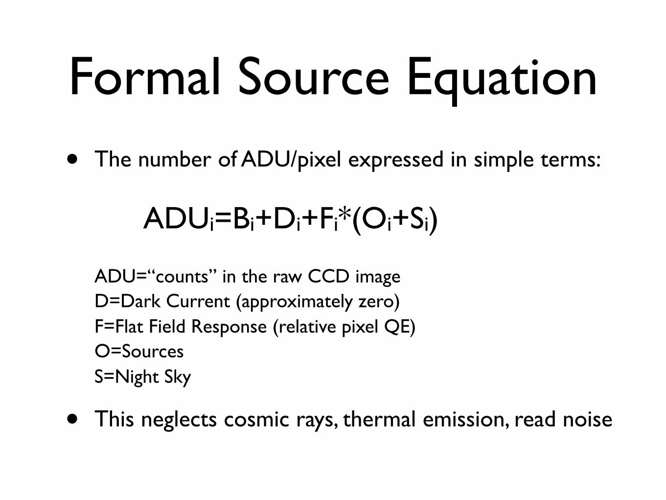
Formal Source Equation• The number of ADU/pixel expressed in simple terms:

ADUi=Bi+Di+Fi*(Oi+Si)

ADU=“counts” in the raw CCD imageD=Dark Current (approximately zero) F=Flat Field Response (relative pixel QE) O=Sources S=Night Sky

• This neglects cosmic rays, thermal emission, read noise

Types of Effects

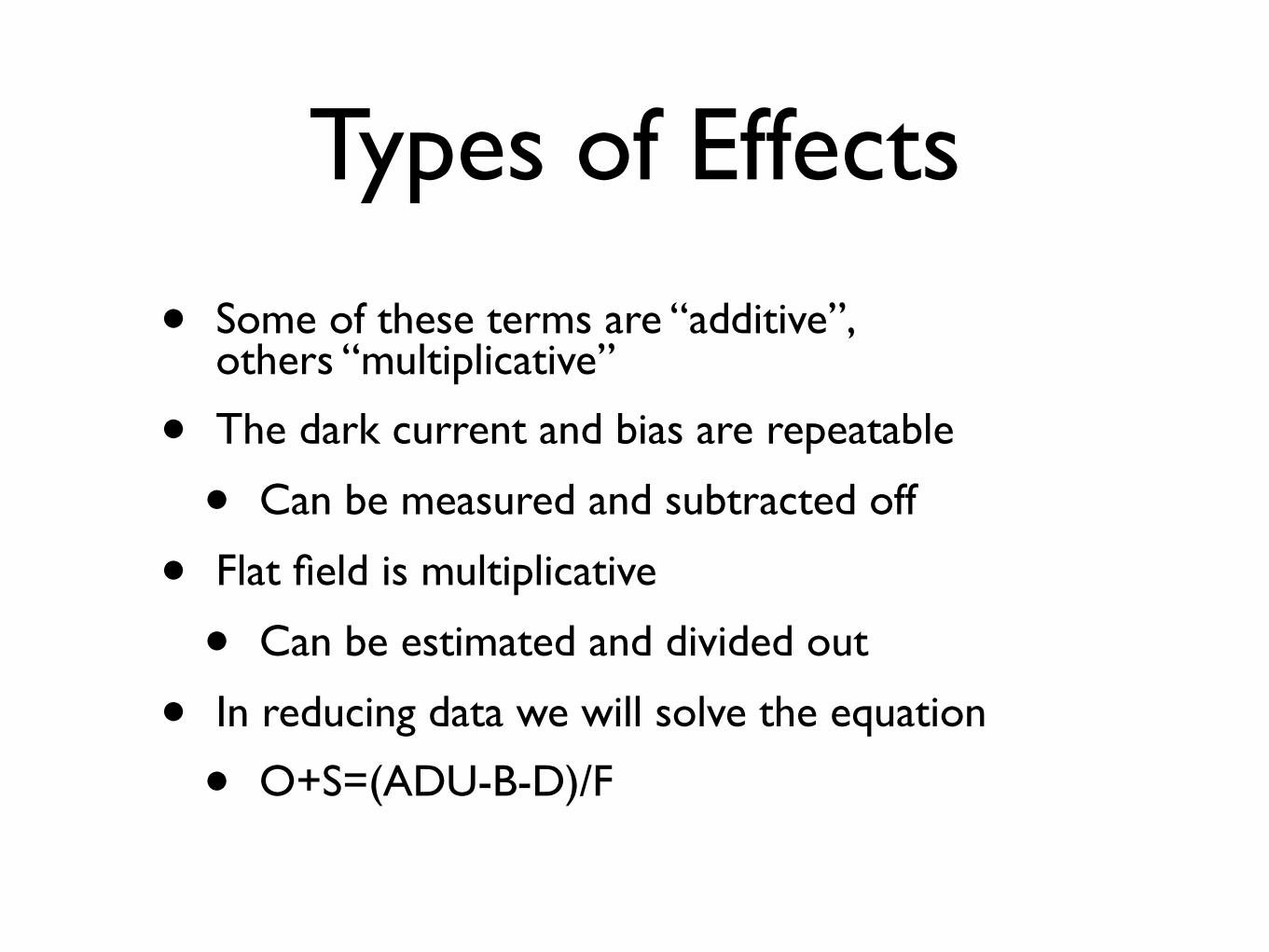
• Some of these terms are “additive”, others “multiplicative”

• The dark current and bias are repeatable

• Can be measured and subtracted off

• Flat field is multiplicative

• Can be estimated and divided out

• In reducing data we will solve the equation

• O+S=(ADU-B-D)/F

Reducing data with Python

• Python is the standard language we’ve been learning.

• Python is installed on both your own and the observatory computers

• Will use archival data today

• Reduce our own 16” CCD data next week

Python and arrays

• Complete the exercises athttp://python-astro.blogspot.com/2012/05/playing-with-arrays-slicing-sorting.html

• Get comfortable with creating, slicing, and manipulating arrays in Python.

Our Sample Data

• I have made a small package of images we can work with today

• Download these images to your own directory http://www.phyast.pitt.edu/~wmwv/Classes/A1263/Labs/Lab2/images/

• Figure out how to let ds9 and Python see that new directory

Viewing our data

• Let’s take a look at what we have

• There should be - A bias- A flat - A mask file - An image (of a SN)

• Download ds9 from http://hea-www.harvard.edu/RD/ds9/

• Look at each of the files using ds9

A friend: lab1.py

• There is a file that will be a good reference called lab1.py

• It’s an Python procedure and has examplesof all of the basic steps for calibration

• Use your favorite editor to look at it

FITS files

• CCD data are usually stored in FITS files

• Binary format to represent data in each pixel

• (usually 16 or 32 bit)

• Also includes a header with useful information

• From Python tryimport pyfits as py bias=pyfits.getdata('BIAS.fits')

• Plot slices through the image and compare to the image displayed by ds9.

Raw Images

• Have a look at the SN image with ds9

• Looks pretty ratty!

• What about the black columns and rows?

• Why does each quadrant look different?

• Do you see any stars?

Flat Field• Have a look at the flat field image with ds9

• Exposure of evenly illuminated screen

• If detector and telescope were perfect every pixel would have the same value

• There is lots of structure due to

• Pixel QE

• Optical problems

• Dust, fingerprints, insects, etc.

Oi+Si=(ADUi-Bi-Di)/Fi

• The first step in solving the above equation is to subtract the bias from our images

• Python makes this easy with matrix operations

• Load the bias, flat, and sn images into arrays

• Subtract the bias image from the flat and sn

• Take a look at the flat and SN image now.

• It’s probably a good idea to “mask out” those columns and rows that contain no data

• Pre-made mask for us called kepcam_mask.fits

Flat Field• The flat field must be normalized

• Sticking something with an average value of 104 into our reduction equation is not really what we want

• We’re interested in the relative sensitivity (including optical effects) of each pixel

• The flat field must be “normalized” to have an average value 1.0

• Use the “plothist” command to look at the distribution of the pixels…not very uniform at all!

• Take a look at the mean and median of the values

• You can also try a clipped mean

• Let’s normalize the flat by 9561.9

Next Step• Plot part of the flat field…I see 40% variations

• If we assume that the dark current is 0.0 electrons/second we are now ready to complete the process Oi+Si=(ADUi-Bi-Di)/Fi• What does that image look like?

• Have a look at in ds9 (try setting the range to [800, 3000] and using Log scaling)

• Pretty good, no?

What Else?• We ignored cosmic rays, which can be important

for long exposures with thick CCDs

• This exposure was only 240 seconds

• You can see the fringing pattern in the image. We neglected this here

• In general the normalized flat would be made from many flats in order to minimize cosmic rays, etc.

• The bleed trail on the bright star at left should be masked

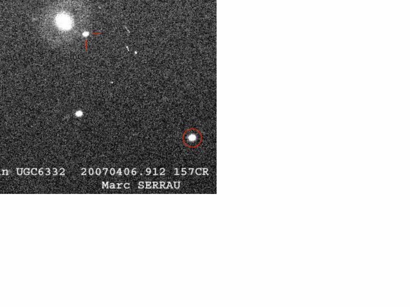
Science! • The SN in this frame is in a pretty galaxy

near [416,1550]

• Zoom in, stretch the display and lots of interesting galaxy structure will emerge

• Have a look at a bright star…what’s does the plot across a bright star look like?

• The SN should be near RA: 11:19:14.57 Dec: +20:48:32.5

• Zoom and stretch your display to match the image on the following page.