Embed Size (px)
Citation preview
Basic Theory of ODE and Vector Fields
Michael E. Taylor
Contents0. Introduction1. The derivative2. Fundamental local existence theorem for ODE3. Inverse function and implicit function theorem4. Constant-coefficient linear systems; exponentiation of matrices5. Variable-coefficient systems of ODE; Duhamel’s formula6. Dependence of solutions on initial data and on other parameters7. Flows and vector fields8. Lie brackets9. Commuting flows; Frobenius’s theorem10. Hamiltonian systems11. Geodesics12. Variational problems and the stationary action principle13. Differential forms14. The symplectic form and canonical transformations15. First-order, scalar, nonlinear PDE16. Completely integrable Hamiltonian systems17. Examples of integrable systems; central force problems18. Relativistic motion19. Topological applications of differential forms20. Critical points and index of a vector fieldA. Nonsmooth vector fields
Introduction
This text examines basic topics in the field of ordinary differential equations(ODE), as it has developed from the era of Newton into modern times. Thisis closely tied to the development of a number of concepts in advancedcalculus. We begin with a brief discussion of the derivative of a vector-valued function of several variables as a linear map. We then establish in§2 the fundamental local existence and uniqueness of solutions to ODE, ofthe form
(0.1)dy
dt= F (t, y), y(t0) = y0,
2
where F (t, y) is continuous in both arguments and Lipschitz in y, and ytakes values in Rk. The proof uses a nice tool known as the contractionmapping principle; next we use this principle to establish the inverse andimplicit function theorems in §3. After a discussion of constant-coefficientlinear equations, in which we recall the basic results of linear algebra, in §4,we treat variable-coefficient linear ODE in §5, emphasizing a result knownas Duhamel’s principle, and then use this to examine smooth dependenceon parameters for solutions to nonlinear ODE in §6.
The first six sections have a fairly purely analytic character and presentODE from a perspective similar to that seen in introductory courses. It isexpected that the reader has seen much of this material before. Beginningin §7, the material begins to acquire a geometrical flavor as well. Thissection interprets solutions to (0.1) in terms of a flow generated by a vectorfield. The next two sections examine the Lie derivative of vector fields andsome of its implications for ODE. While we initially work on domains inRn, here we begin a transition to global constructions, involving workingon manifolds and hence making use of concepts that are invariant underchanges of coordinates. By the end of §13, this transition is complete.Appendix B collects some of the basic facts about manifolds which areuseful for such an approach to analysis.
Physics is a major source of differential equations, and in §10 we dis-cuss some of the basic ODE arising from Newton’s force law, convertingthe resulting second-order ODE to first-order systems known as Hamilton-ian systems. The study of Hamiltonian vector fields is a major focus forthe subsequent sections in this chapter. In §11 we deal with an appar-ently disjoint topic, the equations of geodesics on a Riemannian manifold.We introduce the covariant derivative as a tool for expressing the geodesicequations, and later show that these equations can also be cast in Hamil-tonian form. In §12 we study a general class of variational problems, givingrise to both the equations of mechanics and the equations of geodesics, allexpressible in Hamiltonian form.
In §13 we develop the theory of differential forms, one of E. Cartan’sgreat contributions to analysis. There is a differential operator, calledthe exterior derivative, acting on differential forms. In beginning coursesin multivariable calculus, one learns of div, grad, and curl as the majorfirst-order differential operators; from a more advanced perspective, it isreasonable to think of the Lie derivative, the covariant derivative, and theexterior derivative as filling this role. The relevance of differential forms toODE has many roots, but its most direct relevance for Hamiltonian systemsis through the symplectic form, discussed in §14.
Results on Hamiltonian systems are applied in §15 to the study of first-order nonlinear PDE for a single unknown. The next section studies “com-pletely integrable” systems, reversing the perspective, to apply solutions tocertain nonlinear PDE to the study of Hamiltonian systems. These two sec-tions comprise what is known as Hamilton-Jacobi theory. In §17 we make
1. The derivative 3
a further study of integrable systems arising from central force problems,particularly the one involving the gravitational attraction of two bodies, thesolution to which was Newton’s triumph. Section 18 gives a brief relativis-tic treatment of the equations of motion arising from the electromagneticforce, which ushered in Einstein’s theory of relativity.
In §19 we apply material from §13 on differential forms to some topo-logical results, such as the Brouwer fixed-point theorem, the study of thedegree of a map between compact oriented manifolds, and the Jordan-Brouwer separation theorem. We apply the degree theory in §20 to a studyof the index of a vector field, which reflects the behavior of its criticalpoints.
The appendix at the end of this text discusses the existence and unique-ness of solutions to (0.1) when F satisfies a condition weaker than Lipschitzin y. Results established here are applicable to the study of ideal fluid flow,as will be seen in Chapter 17.
1. The derivative
Let O be an open subset of Rn, and let F : O → Rm be a continuousfunction. We say that F is differentiable at a point x ∈ O, with derivativeL, if L : Rn → Rm is a linear transformation such that, for small y ∈ Rn,
(1.1) F (x + y) = F (x) + Ly + R(x, y),
with
(1.2)‖R(x, y)‖‖y‖ → 0 as y → 0.
We denote the derivative at x by DF (x) = L. With respect to the standardbases of Rn and Rm, DF (x) is simply the matrix of partial derivatives,
(1.3) DF (x) =(∂Fj
∂xk
),
so that, if v = (v1, . . . , vn) (regarded as a column vector), then
(1.4) DF (x)v =(∑
k
∂F1
∂xkvk, . . . ,
∑
k
∂Fm
∂xkvk
).
It will be shown that F is differentiable whenever all the partial derivativesexist and are continuous on O. In such a case we say that F is a C1-function on O. In general, F is said to be Ck if all its partial derivativesof order ≤ k exist and are continuous.
In (1.2) we can use the Euclidean norm on Rn and Rm. This norm isdefined by
(1.5) ‖x‖ =(x2
1 + · · ·+ x2n
)1/2

4
for x = (x1, . . . , xn) ∈ Rn. Any other norm would do equally well. Somebasic results on the Euclidean norm are derived in §4.
More generally, the definition of the derivative given by (1.1) and (1.2)extends to a function F : O → Y , where O is an open subset of X, andX and Y are Banach spaces. Basic material on Banach spaces appearsin Appendix A, Functional Analysis. In this case, we require L to be abounded linear map from X to Y . The notion of differentiable function inthis context is useful in the study of nonlinear PDE.
We now derive the chain rule for the derivative. Let F : O → Rm bedifferentiable at x ∈ O, as above; let U be a neighborhood of z = F (x) inRm; and let G : U → Rk be differentiable at z. Consider H = G F . Wehave
(1.6)
H(x + y) = G(F (x + y))
= G(F (x) + DF (x)y + R(x, y)
)
= G(z) + DG(z)(DF (x)y + R(x, y)
)+ R1(x, y)
= G(z) + DG(z)DF (x)y + R2(x, y),
with‖R2(x, y)‖
‖y‖ → 0 as y → 0.
Thus G F is differentiable at x, and
(1.7) D(G F )(x) = DG(F (x)) ·DF (x).
This result works equally well if Rn, Rm, and Rk are replaced by generalBanach spaces.
Another useful remark is that, by the fundamental theorem of calculus,applied to ϕ(t) = F (x + ty),
(1.8) F (x + y) = F (x) +∫ 1
0
DF (x + ty)y dt,
provided F is C1. For a typical application, see (6.6).A closely related application of the fundamental theorem of calculus is
that if we assume that F : O → Rm is differentiable in each variableseparately, and that each ∂F/∂xj is continuous on O, then
(1.9)
F (x + y) = F (x) +n∑
j=1
[F (x + zj)− F (x + zj−1)
]
= F (x) +n∑
j=1
Aj(x, y)yj ,
Aj(x, y) =∫ 1
0
∂F
∂xj
(x + zj−1 + tyjej
)dt,
1. The derivative 5
where z0 = 0, zj = (y1, . . . , yj , 0, . . . , 0), and ej is the standard basis ofRn. Now (1.9) implies that F is differentiable on O, as we stated beneath(1.4). As is shown in many calculus texts, by using the mean value theoreminstead of the fundamental theorem of calculus, one can obtain a slightlysharper result. We leave the reconstruction of this argument to the reader.
We now describe two convenient notations to express higher-order deriva-tives of a Ck-function f : Ω → R, where Ω ⊂ Rn is open. In the first, let Jbe a k-tuple of integers between 1 and n; J = (j1, . . . , jk). We set
(1.10) f (J)(x) = ∂jk· · · ∂j1f(x), ∂j =
∂
∂xj.
Also, we set |J | = k, the total order of differentiation. As will be seen inthe exercises, ∂i∂jf = ∂j∂if , provided f ∈ C2(Ω). Hence, if f ∈ Ck(Ω),then ∂jk
· · · ∂j1f = ∂`k· · · ∂`1f whenever `1, . . . , `k is a permutation of
j1, . . . , jk. Thus, another convenient notation to use is the following. Letα be an n-tuple of nonnegative integers, α = (α1, . . . , αn). Then we set
(1.11) f (α)(x) = ∂α11 · · · ∂αn
n f(x), |α| = α1 + · · ·+ αn.
Note that if |J | = |α| = k and f ∈ Ck(Ω), then
(1.12) f (J)(x) = f (α)(x), with αi = #` : j` = i.Correspondingly, there are two expressions for monomials in x:
(1.13) xJ = xj1 · · ·xjk, xα = xα1
1 · · ·xαnn ,
and xJ = xα, provided J and α are related as in (1.12). Both of thesenotations are called “multi-index” notations.
We now derive Taylor’s formula with remainder for a smooth functionF : Ω → R, making use of these multi-index notations. We will apply theone-variable formula,
(1.14) ϕ(t) = ϕ(0) + ϕ′(0)t +12ϕ′′(0)t2 + · · ·+ 1
k!ϕ(k)(0)tk + rk(t),
with
(1.15) rk(t) =1k!
∫ t
0
(t− s)kϕ(k+1)(s) ds,
given ϕ ∈ Ck+1(I), I = (−a, a). Let us assume that 0 ∈ Ω and that theline segment from 0 to x is contained in Ω. We set ϕ(t) = F (tx) and apply(1.14) and (1.15) with t = 1. Applying the chain rule, we have
(1.16) ϕ′(t) =n∑
j=1
∂jF (tx)xj =∑
|J|=1
F (J)(tx)xJ .
Differentiating again, we have
(1.17) ϕ′′(t) =∑
|J|=1,|K|=1
F (J+K)(tx)xJ+K =∑
|J|=2
F (J)(tx)xJ ,
6
where, if |J | = k and |K| = `, we take J + K = (j1, . . . , jk, k1, . . . , k`).Inductively, we have
(1.18) ϕ(k)(t) =∑
|J|=k
F (J)(tx)xJ .
Hence, from (1.14), with t = 1,
F (x) = F (0) +∑
|J|=1
F (J)(0)xJ + · · ·+ 1k!
∑
|J|=k
F (J)(0)xJ + Rk(x),
or, more briefly,
(1.19) F (x) =∑
|J|≤k
1|J |!F
(J)(0)xJ + Rk(x),
where
(1.20) Rk(x) =1k!
∑
|J|=k+1
(∫ 1
0
(1− s)kF (J)(sx) ds)xJ .
This gives Taylor’s formula with remainder for F ∈ Ck+1(Ω), in the J-multi-index notation.
We also want to write the formula in the α-multi-index notation. Wehave
(1.21)∑
|J|=k
F (J)(tx)xJ =∑
|α|=k
ν(α)F (α)(tx)xα,
where
(1.22) ν(α) = #J : α = α(J),and we define the relation α = α(J) to hold provided (1.12) holds or,equivalently, provided xJ = xα. Thus, ν(α) is uniquely defined by
(1.23)∑
|α|=k
ν(α)xα =∑
|J|=k
xJ = (x1 + · · ·+ xn)k.
One sees that, if |α| = k, then ν(α) is equal to the product of the numberof combinations of k objects, taken α1 at a time, times the number ofcombinations of k − α1 objects, taken α2 at a time, and so on, times thenumber of combinations of k − (α1 + · · · + αn−1) objects, taken αn at atime. Thus(1.24)
ν(α) =(
k
α1
)(k − α1
α2
)· · ·
(k − α1 − · · · − αn−1
αn
)=
k!α1!α2! · · ·αn!
.
In other words, for |α| = k,
(1.25) ν(α) =k!α!
, where α! = α1! · · ·αn!.

Exercises 7
Thus, the Taylor formula (1.19) can be rewritten as
(1.26) F (x) =∑
|α|≤k
1α!
F (α)(0)xα + Rk(x),
where
(1.27) Rk(x) =∑
|α|=k+1
k + 1α!
(∫ 1
0
(1− s)kF (α)(sx) ds)xα.
Exercises
1. Let Mn×n be the space of complex n × n matrices, and let det : Mn×n → Cdenote the determinant. Show that if I is the identity matrix, then
D det(I)B = Tr B,
i.e.,
d
dtdet(I + tB)|t=0 = Tr B.
2. If A(t) =(ajk(t)
)is a curve in Mn×n, use the expansion of (d/dt) det A(t) as
a sum of n determinants, in which the rows of A(t) are successively differen-tiated, to show that, for A ∈ Mn×n,
D det(A)B = Tr(Cof(A)t ·B
),
where Cof(A) is the cofactor matrix of A.3. Suppose A ∈ Mn×n is invertible. Using
det(A + tB) = (det A) det(I + tA−1B),
show that
D det(A)B = (det A) Tr (A−1B).
Comparing the result of Exercise 2, deduce Cramer’s formula:
(1.28) (det A)A−1 = Cof(A)t.
4. Identify R2 and C via z = x + iy. Then multiplication by i on C correspondsto applying
J =
(0 −11 0
).
Let O ⊂ R2 be open, and let f : O → R2 be C1. Say f = (u, v). RegardDf(x, y) as a 2×2 real matrix. One says f is holomorphic, or complex analytic,provided the Cauchy-Riemann equations hold:
(1.29)∂u
∂x=
∂v
∂y,
∂u
∂y= −∂v
∂x.
8
Show that this is equivalent to the condition
Df(x, y)J = JDf(x, y).
Generalize to O open in Cm, f : O → Cn.5. If R(x) is a C∞-function near the origin in Rn, satisfying R(0) = 0 and
DR(0) = 0, show that there exist smooth functions rjk(x) such that
R(x) =∑
rjk(x)xjxk.
(Hint: Using (1.8), write R(x) = Φ(x)x, Φ(x) =∫ 1
0DR(tx)dt, since R(0) = 0.
Then Φ(0) = DR(0) = 0, so (1.8) can be applied again, to give Φ(x) = Ψ(x)x.)6. If f is C1 on a region in R2 containing [a, b]× y, show that
d
dy
∫ b
a
f(x, y) dx =
∫ b
a
∂f
∂y(x, y) dx.
(Hint: Show that the left side is equal to
limh→0
∫ b
a
1
h
∫ h
0
∂f
∂y(x, y + s) ds dx.)
7. Suppose F : O → Rm is a C2-function. Applying the fundamental theorem ofcalculus, first to
Gj(x) = F (x + hej)− F (x)
(as a function of h) and then to
Hjk(x) = Gj(x + hek)−Gj(x),
where ej is the standard basis of Rn, show that if x ∈ O and h is small,then
F (x + hej + hek)− F (x + hek)− F (x + hej) + F (x)
=
∫ h
0
∫ h
0
∂
∂xk
∂F
∂xj
(x + sej + tek
)ds dt.
Similarly, show that this quantity is equal to∫ h
0
∫ h
0
∂
∂xj
∂F
∂xk
(x + sej + tek
)dt ds.
Deduce that
∂
∂xk
∂F
∂xj(x) =
∂
∂xj
∂F
∂xk(x).
(Hint: Use Exercise 6.)Arguments that use the mean value theorem instead of the fundamental the-orem of calculus can be found in many calculus texts.
2. Fundamental local existence theorem for ODE
The goal of this section is to establish the existence of solutions to an ODE:
(2.1)dy
dt= F (t, y), y(t0) = y0.
2. Fundamental local existence theorem for ODE 9
We will prove the following fundamental result.
Theorem 2.1. Let y0 ∈ O, an open subset of Rn, I ⊂ R an intervalcontaining t0. Suppose F is continuous on I×O and satisfies the followingLipschitz estimate in y:
(2.2) ‖F (t, y1)− F (t, y2)‖ ≤ L‖y1 − y2‖,for t ∈ I, yj ∈ O. Then the equation (2.1) has a unique solution on somet-interval containing t0.
To begin the proof, we note that the equation (2.1) is equivalent to theintegral equation
(2.3) y(t) = y0 +∫ t
t0
F (s, y(s)) ds.
Existence will be established via the Picard iteration method, which is thefollowing. Guess y0(t), e.g., y0(t) = y0. Then set
(2.4) yk(t) = y0 +∫ t
t0
F(s, yk−1(s)
)ds.
We aim to show that, as k →∞, yk(t) converges to a (unique) solution of(2.3), at least for t close enough to t0. To do this, we will use the followingtool, known as the contraction mapping principle.
Theorem 2.2. Let X be a complete metric space, and let T : X → Xsatisfy
(2.5) dist(Tx, Ty) ≤ r dist(x, y),
for some r < 1. (We say that T is a contraction.) Then T has a uniquefixed point x. For any y0 ∈ X, T ky0 → x as k →∞.
Proof. Pick y0 ∈ X, and let yk = T ky0. Then
dist (yk+1, yk) ≤ rk dist (y1, y0),
so
(2.6)
dist(yk+m, yk) ≤ dist(yk+m, yk+m−1) + · · ·+ dist(yk+1, yk)
≤ (rk + · · ·+ rk+m−1
)dist(y1, y0)
≤ rk(1− r
)−1 dist(y1, y0).
It follows that (yk) is a Cauchy sequence, so it converges; yk → x. SinceTyk = yk+1 and T is continuous, it follows that Tx = x, that is, x is afixed point. The uniqueness of the fixed point is clear from the estimatedist(Tx, Tx′) ≤ r dist(x, x′), which implies dist(x, x′) = 0 if x and x′ arefixed points. This completes the proof.

10
Tackling the solvability of (2.3), we look for a fixed point of T , definedby
(2.7) (Ty)(t) = y0 +∫ t
t0
F (s, y(s)) ds.
Let
(2.8) X =u ∈ C(J,Rn) : u(t0) = y0, sup
t∈J‖u(t)− y0‖ ≤ K
.
Here J = [t0 − ε, t0 + ε], where ε will be chosen, sufficiently small, below.K is picked so y : ‖y − y0‖ ≤ K is contained in O, and we also supposeJ ⊂ I. Then there exists an M such that
(2.9) sups∈J,‖y−y0‖≤K
‖F (s, y)‖ ≤ M.
Then, provided
(2.10) ε ≤ K
M,
we have
(2.11) T : X → X.
Now, using the Lipschitz hypothesis (2.2), we have, for t ∈ J ,
(2.12) ‖(Ty)(t)−(Tz)(t)‖ ≤∫ t
t0
L‖y(s)−z(s)‖ ds ≤ ε L sups∈J
‖y(s)−z(s)‖,
assuming y and z belong to X. It follows that T is a contraction on Xprovided one has
(2.13) ε <1L
,
in addition to the hypotheses above. This proves Theorem 2.1.In view of the lower bound on the length of the interval J on which the
existence theorem works, it is easy to show that the only way a solutioncan fail to be globally defined, that is, to exist for all t ∈ I, is for y(t) to“explode to infinity” by leaving every compact set K ⊂ O, as t → t1, forsome t1 ∈ I.
We remark that the local existence proof given above works if Rn isreplaced by any Banach space.
Often one wants to deal with a higher-order ODE. There is a standardmethod of reducing an nth-order ODE
(2.14) y(n)(t) = f(t, y, y′, . . . , y(n−1))
to a first-order system. One sets u = (u0, . . . , un−1), with
(2.15) u0 = y, uj = y(j),
Exercises 11
and then
(2.16)du
dt=
(u1, . . . , un−1, f(t, u0, . . . , un−1)
)= g(t, u).
If y takes values in Rk, then u takes values in Rkn.If the system (2.1) is nonautonomous, that is, if F explicitly depends
on t, it can be converted to an autonomous system (one with no explicitt-dependence) as follows. Set z = (t, y). We then have
(2.17) z′ = (1, y′) = (1, F (z)) = G(z).
Sometimes this process destroys important features of the original system(2.1). For example, if (2.1) is linear, (2.17) might be nonlinear. Neverthe-less, the trick of converting (2.1) to (2.17) has some uses.
Many systems of ODE are difficult to solve explicitly. One very basicclass of ODE can be solved explicitly, in terms of integrals, namely thesingle first-order linear ODE:
(2.18)dy
dt= a(t)y + b(t), y(0) = y0,
where a(t) and b(t) are continuous real- or complex-valued functions. Set
(2.19) A(t) =∫ t
0
a(s) ds.
Then (2.18) can be written as
(2.20) eA(t) d
dt
(e−A(t)y
)= b(t),
which yields
(2.21) y(t) = eA(t)y0 + eA(t)
∫ t
0
e−A(s)b(s) ds.
Compare this result with formulas (4.42) and (5.8), in subsequent sectionsof this chapter.
Exercises
1. Solve the initial-value problem
y′ = y2, y(0) = a,
given a ∈ R. On what t-interval is the solution defined?2. Under the hypotheses of Theorem 2.1, if y solves (2.1) for t ∈ [T0, T1], and
y(t) ∈ K, compact in O, for all such t, prove that y(t) extends to a solutionfor t ∈ [S0, S1], with S0 < T0, T1 > T0, as stated beneath (2.13).
3. Let M be a compact, smooth surface in Rn. Suppose F : Rn → Rn is asmooth map (vector field) such that, for each x ∈ M, F (x) is tangent to M ,
12
that is, the line γx(t) = x + tF (x) is tangent to M at x, at t = 0. Show thatif x ∈ M , then the initial-value problem
y′ = F (y), y(0) = x
has a solution for all t ∈ R, and y(t) ∈ M for all t.(Hint: Locally, straighten out M to be a linear subspace of Rn, to which F istangent. Use uniqueness. Material in §3 will help do this local straightening.)Reconsider this problem after reading §7.
4. Show that the initial-value problem
dx
dt= −x(x2 + y2),
dy
dt= −y(x2 + y2), x(0) = x0, y(0) = y0
has a solution for all t ≥ 0, but not for all t < 0, unless (x0, y0) = (0, 0).
3. Inverse function and implicit function theorems
We will use the contraction mapping principle to establish the inverse func-tion theorem, which together with its corollary, the implicit function the-orem, is a fundamental result in multivariable calculus. First we state theinverse function theorem.
Theorem 3.1. Let F be a Ck-map from an open neighborhood Ω of p0 ∈Rn to Rn, with q0 = F (p0). Suppose the derivative DF (p0) is invertible.Then there is a neighborhood U of p0 and a neighborhood V of q0 suchthat F : U → V is one-to-one and onto, and F−1 : V → U is a Ck-map.(One says that F : U → V is a diffeomorphism.)
Proof. Using the chain rule, it is easy to reduce to the case p0 = q0 = 0and DF (p0) = I, the identity matrix, so we suppose this has been done.Thus,
(3.1) F (u) = u + R(u), R(0) = 0, DR(0) = 0.
For v small, we want to solve
(3.2) F (u) = v.
This is equivalent to u + R(u) = v, so let
(3.3) Tv(u) = v −R(u).
Thus, solving (3.2) is equivalent to solving
(3.4) Tv(u) = u.
We look for a fixed point u = K(v) = F−1(v). Also, we want to provethat DK(0) = I, that is, that K(v) = v + r(v), with r(v) = o(‖v‖). If wesucceed in doing this, it follows easily that, for general x close to 0,
DK(x) =(DF
(K(x)
))−1
,
3. Inverse function and implicit function theorems 13
and a simple inductive argument shows that K is Ck if F is Ck. Nowconsider
(3.5) Tv : Xv −→ Xv,
with
(3.6) Xv = u ∈ Ω : ‖u− v‖ ≤ Av,where we set
(3.7) Av = sup‖w‖≤2‖v‖
‖R(w)‖.
We claim that (3.5) holds if ‖v‖ is sufficiently small. To prove this, notethat Tv(u) − v = −R(u), so we need to show that, provided ‖v‖ is small,u ∈ Xv implies ‖R(u)‖ ≤ Av. But indeed, if u ∈ Xv, then ‖u‖ ≤ ‖v‖+Av,which is ≤ 2‖v‖ if ‖v‖ is small, so then
‖R(u)‖ ≤ sup‖w‖≤2‖v‖
‖R(w)‖ = Av;
this establishes (3.5).Note that if ‖v‖ is small enough, the map (3.5) is a contraction map,
so there exists a unique fixed point u = K(v) ∈ Xv. Also note that sinceu ∈ Xv,
(3.8) ‖K(v)− v‖ ≤ Av = o(‖v‖).Hence, the inverse function theorem is proved.
Thus, if DF is invertible on the domain of F , then F is a local diffeo-morphism, although stronger hypotheses are needed to guarantee that Fis a global diffeomorphism onto its range. Here is one result along theselines.
Proposition 3.2. If Ω ⊂ Rn is open and convex, F : Ω → Rn is C1, andthe symmetric part of DF (u) is positive-definite for each u ∈ Ω, then F isone-to-one on Ω.
Proof. Suppose that F (u1) = F (u2), where u2 = u1 + w. Consider ϕ :[0, 1] → R, given by
ϕ(t) = w · F (u1 + tw).
Thus ϕ(0) = ϕ(1), so ϕ′(t0) must vanish for some t0 ∈ (0, 1), by the meanvalue theorem. But ϕ′(t) = w · DF (u1 + tw)w > 0, if w 6= 0, by thehypothesis on DF . This shows that F is one-to-one.
We can obtain the following implicit function theorem as a consequenceof the inverse function theorem.
14
Theorem 3.3. Suppose U is a neighborhood of x0 ∈ Rk, V is a neighbor-hood of z0 ∈ R`, and
(3.9) F : U × V −→ R`
is a Ck-map. Assume DzF (x0, z0) is invertible; say F (x0, z0) = u0. Thenthe equation F (x, z) = u0 defines z = f(x, u0) for x near x0, with f aCk-map.
Proof. Consider H : U × V → Rk × R` defined by
(3.10) H(x, z) =(x, F (x, z)
).
We have
(3.11) DH =(
I DxF0 DzF
).
Thus DH(x0, z0) is invertible, so J = H−1 exists and is Ck, by the inversefunction theorem. It is clear that J(x, u0) has the form
(3.12) J(x, u0) =(x, f(x, u0)
),
and f is the desired map.
As in §2, we remark that the inverse function theorem generalizes. Onecan replace Rn by any Banach space and the proof of Theorem 3.1 givenabove extends with no change. Such generalizations are useful in nonlinearPDE, as we will see in Chapter 14.
Exercises
1. Suppose that F : U → Rn is a C2-map, U is open in Rn, p ∈ U , and DF (p)is invertible. With q = F (p), define a map N on a neighborhood of p by
(3.13) N(x) = x + DF (x)−1(q − F (x)
).
Show that there exists ε > 0 and C < ∞ such that, for 0 ≤ r < ε,
‖x− p‖ ≤ r =⇒ ‖N(x)− p‖ ≤ C r2.
Conclude that if ‖x1 − p‖ ≤ r, with r < min(ε, 1/2C), then xj+1 = N(xj)defines a sequence converging very rapidly to p. This is the basis of Newton’smethod, for solving F (p) = q for p.(Hint: Write x = p+y, F (x) = F (p)+DF (x)y+R, with R given as in (1.27),with k = 2. Then N(x) = p + y, y = −DF (x)−1R.)
2. Applying Newton’s method to f(x) = 1/x, show that you get a fast approxi-mation to division using only addition and multiplication.(Hint: Carry out the calculation of N(x) in this case and notice a “miracle.”)
4. Constant-coefficient linear systems; exponentiation of matrices 15
3. Identify R2n with Cn via z = x + iy, as in Exercise 4 of §1. Let U ⊂ R2n
be open, and let F : U → R2n be C1. Assume that p ∈ U and DF (p) isinvertible. If F−1 : V → U is given as in Theorem 3.1, show that F−1 isholomorphic provided F is.
4. Let O ⊂ Rn be open. We say that a function f ∈ C∞(O) is real analyticprovided that, for each x0 ∈ O, we have a convergent power-series expansion
(3.14) f(x) =∑
α≥0
1
α!f (α)(x0)(x− x0)
α,
valid in a neighborhood of x0. Show that we can let x be complex in (3.14), andobtain an extension f to a neighborhood of O in Cn. Show that the extendedfunction is holomorphic, that is, satisfies the Cauchy-Riemann equations.Remark. It can be shown that, conversely, any holomorphic function has apower-series expansion. See (2.30) of Chapter 3 for one such proof. For thenext exercise, assume this to be known.
5. Let O ⊂ Rn be open, p ∈ O, and f : O → Rn be real analytic, with Df(p)invertible. Take f−1 : V → U as in Theorem 3.1. Show f−1 is real analytic.(Hint: Consider a holomorphic extension F : Ω → Cn of f , and apply Exercise3.)
4. Constant-coefficient linear systems; exponentiation ofmatrices
Let A be an n× n matrix, real or complex. We consider the linear ODE
(4.1) y′ = Ay, y(0) = y0.
In analogy to the scalar case, we can produce the solution in the form
(4.2) y(t) = etAy0,
where we define the matrix exponential
(4.3) etA =∞∑
k=0
tk
k!Ak.
We will establish estimates implying the convergence of this infinite seriesfor all real t, indeed for all complex t. Then term-by-term differentiation isvalid and gives (4.1). To discuss convergence of (4.3), we need the notion ofthe norm of a matrix. This is a special case of results discussed in AppendixA, Functional Analysis.
If u = (u1, . . . , un) belongs to Rn or to Cn, set, as in (1.5),
(4.4) ‖u‖ =(|u1|2 + · · ·+ |un|2
)1/2.
Then, if A is an n× n matrix, set
(4.5) ‖A‖ = sup‖Au‖ : ‖u‖ ≤ 1.

16
The norm (4.4) possesses the following properties:
‖u‖ ≥ 0, ‖u‖ = 0 if and only if u = 0,(4.6)
‖cu‖ = |c| ‖u‖, for real or complex c,(4.7)
‖u + v‖ ≤ ‖u‖+ ‖v‖.(4.8)
The last property, known as the triangle inequality, follows from Cauchy’sinequality:
(4.9) |(u, v)| ≤ ‖u‖ · ‖v‖,where the inner product is (u, v) = u1v1 + · · ·+unvn. To deduce (4.8) from(4.9), just square both sides of (4.8). To prove (4.9), use (u− v, u− v) ≥ 0to get
2 Re (u, v) ≤ ‖u‖2 + ‖v‖2.Then replace u by eiθu to deduce
2|(u, v)| ≤ ‖u‖2 + ‖v‖2.Next, replace u by tu and v by t−1v, to get
2|(u, v)| ≤ t2‖u‖2 + t−2‖v‖2,for any t > 0. Picking t so that t2 = ‖v‖/‖u‖, we have Cauchy’s inequality(4.9).
Given (4.6)–(4.8), we easily get
(4.10)‖A‖ ≥ 0,
‖cA‖ = |c| ‖A‖,‖A + B‖ ≤ ‖A‖+ ‖B‖.
Also, ‖A‖ = 0 if and only if A = 0. The fact that ‖A‖ is the smallestconstant K such that ‖Au‖ ≤ K‖u‖ gives
(4.11) ‖AB‖ ≤ ‖A‖ · ‖B‖.In particular,
(4.12) ‖Ak‖ ≤ ‖A‖k.
This makes it easy to check the convergence of the power-series (4.3).Power-series manipulations can be used to establish the identity
(4.13) esAetA = e(s+t)A.
Another way to prove this is as follows. Regard t as fixed; denote the leftside of (4.13) as X(s) and the right side as Y (s). Then differentiation withrespect to s gives, respectively,
(4.14)X ′(s) = AX(s), X(0) = etA,
Y ′(s) = AY (s), Y (0) = etA,
4. Constant-coefficient linear systems; exponentiation of matrices 17
so the uniqueness of solutions to the ODE implies X(s) = Y (s) for all s.We note that (4.13) is a special case of the following.
Proposition 4.1. et(A+B) = etAetB for all t, if and only if A and Bcommute.
Proof. Let
(4.15) Y (t) = et(A+B), Z(t) = etAetB .
Note that Y (0) = Z(0) = I, so it suffices to show that Y (t) and Z(t) satisfythe same ODE, to deduce that they coincide. Clearly,
(4.16) Y ′(t) = (A + B)Y (t).
Meanwhile,
(4.17) Z ′(t) = AetAetB + etABetB .
Thus we get the equation (4.16) for Z(t) provided we know that
(4.18) etAB = BetA if AB = BA.
This follows from the power-series expansion for etA, together with the factthat
(4.19) AkB = BAk, ∀ k ≥ 0, if AB = BA.
For the converse, if Y (t) = Z(t) for all t, then etAB = BetA, by (4.17),and hence, taking the t-derivative, etAAB = BAetA; setting t = 0 givesAB = BA.
If A is in diagonal form,
(4.20) A =
a1
. . .an
,
then clearly
(4.21) etA =
eta1
. . .etan
.
The following result makes it useful to diagonalize A in order to computeetA.
Proposition 4.2. If K is an invertible matrix and B = KAK−1, then
(4.22) etB = K etA K−1.
18
Proof. This follows from the power-series expansion (4.3), given the ob-servation that
(4.23) Bk = K Ak K−1.
In view of (4.20)–(4.22), it is convenient to record a few standard resultsabout eigenvalues and eigenvectors here. Let A be an n × n matrix overF, F = R or C. An eigenvector of A is a nonzero u ∈ Fn such that
(4.24) Au = λu,
for some λ ∈ F . Such an eigenvector exists if and only if A−λI : Fn → Fn
is not invertible, that is, if and only if
(4.25) det(A− λI) = 0.
Now (4.25) is a polynomial equation, so it always has a complex root. Thisproves the following.
Proposition 4.3. Given an n × n matrix A, there exists at least one(complex) eigenvector u.
Of course, if A is real, and we know there is a real root of (4.25) (e.g., ifn is odd), then a real eigenvector exists. One important class of matricesguaranteed to have real eigenvalues is the class of self-adjoint matrices. Theadjoint of an n × n complex matrix is specified by the identity (Au, v) =(u, A∗v).
Proposition 4.4. If A = A∗, then all eigenvalues of A are real.
Proof. Au = λu implies
(4.26) λ‖u‖2 = (λu, u) = (Au, u) = (u,Au) = (u, λu) = λ‖u‖2.Hence λ = λ, if u 6= 0.
We now establish the following important result.
Theorem 4.5. If A = A∗, then there is an orthonormal basis of Cn con-sisting of eigenvectors of A.
Proof. Let u1 be one unit eigenvector; Au1 = λu1. Existence is guaran-teed by Proposition 4.3. Let V = (u1)⊥ be the orthogonal complement ofthe linear span of u1. Then dim V is n− 1 and
(4.27) A : V → V, if A = A∗.
The result follows by induction on n.
4. Constant-coefficient linear systems; exponentiation of matrices 19
Corollary 4.6. If A = At is a real symmetric matrix, then there is anorthonormal basis of Rn consisting of eigenvectors of A.
Proof. By Proposition 4.4 and the remarks following Proposition 4.3,there is one unit eigenvector u1 ∈ Rn. The rest of the proof is as above.
The proofs of the last four results rest on the fact that every nonconstantpolynomial has a complex root. This is the fundamental theorem of algebra.A proof is given in §19 (Exercise 5), and another after Corollary 4.7 of
Chapter 3. An alternative approach to Proposition 4.3 when A = A∗,yielding Proposition 4.4–Corollary 4.6, is given in one of the exercises atthe end of this section.
Given an ODE in upper triangular form,
(4.28)dy
dt=
a11 ∗ ∗. . . ∗
ann
y,
you can solve the last ODE for yn, as it is just dyn/dt = annyn. Thenyou get a single nonhomogeneous ODE for yn−1, which can be solved asdemonstrated in (2.18)–(2.21), and you can continue inductively to solve.Thus, it is often useful to be able to put an n × n matrix A in uppertriangular form, with respect to a convenient choice of basis. We willestablish two results along these lines. The first is due to Schur.
Theorem 4.7. For any n × n matrix A, there is an orthonormal basisu1, . . . , un of Cn with respect to which A is in upper triangular form.
This result is equivalent to the following proposition.
Proposition 4.8. For any A, there is a sequence of vector spaces Vj ofdimension j, contained in Cn, with
(4.29) Vn ⊃ Vn−1 ⊃ · · · ⊃ V1
and
(4.30) A : Vj −→ Vj .
To see the equivalence, if we are granted (4.29)–(4.30), pick un⊥Vn−1,a unit vector, then pick un−1 ∈ Vn−1 such that un−1⊥Vn−2, and so forth.Meanwhile, Proposition 4.8 is a simple inductive consequence of the follow-ing result.
Lemma 4.9. For any matrix A acting on Vn, there is a linear subspaceVn−1, of codimension 1, such that A : Vn−1 → Vn−1.
20
Proof. Use Proposition 4.3, applied to A∗. There is a vector v1 such thatA∗v1 = λv1. Let Vn−1 = (v1)⊥. This completes the proof of the lemma,hence of Theorem 4.7.
Let us look more closely at what you can say about solutions to an ODEthat has been put in the form (4.28). As mentioned, we can obtain yj
inductively by solving nonhomogeneous scalar ODE
(4.31)dyj
dt= ajjyj + bj(t),
where bj(t) is a linear combination of yj+1(t), . . . , yn(t), and the formula(2.21) applies, with A(t) = ajjt. We have yn(t) = Ceannt, so bn−1(t) isa multiple of eannt. If an−1,n−1 6= ann, yn−1(t) will be a linear combi-nation of eannt and ean−1,n−1t, but if an−n,n−1 = ann, yn−1(t) may be alinear combination of eannt and teannt. Further integration will involve∫
p(t)eαtdt, where p(t) is a polynomial. That no other sort of function willarise is guaranteed by the following result.
Lemma 4.10. If p(t) ∈ Pn, the space of polynomials of degree ≤ n, andα 6= 0, then
(4.32)∫
p(t)eαt dt = q(t)eαt + C,
for some q(t) ∈ Pn.
Proof. The map p = Tq defined by (d/dt)(q(t)eαt) = p(t)eαt is a map onPn; in fact, we have
(4.33) Tq(t) = αq(t) + q′(t).
It suffices to show that T : Pn → Pn is invertible. But D = d/dt is nilpotenton Pn; Dn+1 = 0. Hence
T−1 = α−1(I + α−1D)−1 = α−1(I − α−1D + · · ·+ α−n(−D)n
).
Note that this gives a neat formula for the integral (4.32). For example,
(4.34)
∫tne−t dt = −(tn + ntn−1 + · · ·+ n!)e−t + C
= −n!(1 + t +
12t2 + · · ·+ 1
n!tn
)e−t + C.
This could also be established by integration by parts and induction. Ofcourse, when α = 0 in (4.32), the result is different; q(t) is a polynomial ofdegree n + 1.
Now the implication for the solution to (4.28) is that all the componentsof y(t) are products of polynomials and exponentials. By Theorem 4.7, we
4. Constant-coefficient linear systems; exponentiation of matrices 21
can draw the same conclusion about the solution to dy/dt = Ay for anyn× n matrix A. We can formally state the result as follows.
Proposition 4.11. For any n× n matrix A,
(4.35) etAv =∑
eλjtvj(t),
where λj is the set of eigenvalues of A and vj(t) are Cn-valued polyno-mials. All the vj(t) are constant when A is diagonalizable.
To see that the λj are the eigenvalues of A, note that in the upper trian-gular case only the exponentials eajjt arise, and in that case the eigenvaluesare precisely the diagonal elements.
If we let Eλ denote the space of Cn-valued functions of the form V (t) =eλtv(t), where v(t) is a Cn-valued polynomial, then Eλ is invariant underthe action of both d/dt and A, hence of d/dt−A. Hence, if a sum V1(t) +· · ·+ Vk(t), Vj(t) ∈ Eλj
(with λjs distinct), is annihilated by d/dt− A, sois each term in this sum.
Therefore, if (4.35) is a sum over the distinct eigenvalues λj of A, itfollows that each term eλjtvj(t) is annihilated by d/dt−A or, equivalently, isof the form etAwj , where wj = vj(0). This leads to the following conclusion.Set
(4.36) Gλ = v ∈ Cn : etAv = etλv(t), v(t) polynomial.Then Cn has a direct-sum decomposition
(4.37) Cn = Gλ1 + · · ·+ Gλk,
where λ1, . . . , λk are the distinct eigenvalues of A. Furthermore, each Gλj
is invariant under A, and
(4.38) Aj = A|Gλjhas exactly one eigenvalue, λj .
This last statement holds because etAv involves only the exponential eλjt,when v ∈ Gλj . We say that Gλj is the generalized eigenspace of A, witheigenvalue λj . Of course, Gλj contains ker (A− λjI). Now Bj = Aj − λjIhas only 0 as an eigenvalue. It is subject to the following result.
Lemma 4.12. If B : Ck → Ck has only 0 as an eigenvalue, then B isnilpotent; in fact,
(4.39) Bm = 0 for some m ≤ k.
Proof. Let Wj = Bj(Ck); then Ck ⊃ W1 ⊃ W2 ⊃ · · · is a sequence offinite-dimensional vector spaces, each invariant under B. This sequencemust stabilize, so for some m, B : Wm → Wm bijectively. If Wm 6= 0, Bhas a nonzero eigenvalue.
22
We next discuss the famous Jordan normal form of a complex n × nmatrix. The result is the following.
Theorem 4.13. If A is an n× n matrix, then there is a basis of Cn withrespect to which A becomes a direct sum of blocks of the form
(4.40)
λj 1
λj. . .
. . . 1λj
.
In light of the decomposition (4.37) and Lemma 4.12, it suffices to es-tablish the Jordan normal form for a nilpotent matrix B. Given v0 ∈ Ck,let m be the smallest integer such that Bmv0 = 0; m ≤ k. If m = k, thenv0, Bv0, . . . , B
m−1v0 gives a basis of Ck, putting B in Jordan normalform. We then say v0 is a cyclic vector for B, and Ck is generated by v0.We call v0, . . . , B
m−1v0 a string.We will have a Jordan normal form precisely if we can write Ck as a direct
sum of cyclic subspaces. We establish that this can be done by inductionon the dimension.
Thus, inductively, we can suppose that W1 = B(Ck) is a direct sumof cyclic subspaces, so W1 has a basis that is a union of strings, let’s saya union of d strings vj , Bvj , . . . , B
`j vj, 1 ≤ j ≤ d. In this case, kerB ∩W1 = N1 has dimension d, and the vectors B`j vj , 1 ≤ j ≤ d, span N1.Furthermore, each vj has the form vj = Bwj for some wj ∈ Ck.
Now dim ker B = k − r ≥ d, where r = dim W1. Let z1, . . . , zk−r−dspan a subspace of ker B complementary to N1. Then the strings wj , vj =Bwj , . . . , B
`j vj, 1 ≤ j ≤ d, and z1, . . . , zk−r−d generate cyclic sub-spaces whose direct sum is Ck, giving the Jordan normal form.
The argument above is part of an argument of Filippov. In fact, Fil-ippov’s proof contains a further clever twist, enabling one to prove Theo-rem 4.13 without using the decomposition (4.37). However, since we gotthis decomposition almost for free as a byproduct of the ODE analysis inProposition 4.11, this author decided to make use of it. See Strang [Str]for Filippov’s proof.
We have seen how constructing etA solves the equation (4.1). We canalso use it to solve a nonhomogeneous equation, of the form
(4.41) y′ = Ay + b(t), y(0) = y0.
Direct calculation shows that the solution is given by
(4.42) y(t) = etAy0 +∫ t
0
e(t−s)A b(s) ds.

Exercises 23
Note how this partially generalizes the formula (2.21). This formula is aspecial case of Duhamel’s principle, which will be discussed further in §5.
We remark that the definition of etA by power series (4.3) extends tothe case where A is a bounded linear operator on a Banach space. In thatcase, etA furnishes the simplest sort of example of a one-parameter group ofoperators. Compare §9 in Appendix A, Functional Analysis, for a furtherdiscussion of semigroups of operators. A number of problems in PDEamount to exponentiating various unbounded operators. The discussion ofeigenvalues, eigenvectors, and normal forms above relies heavily on finitedimensionality, although a good deal of it carries over to compact operatorson infinite-dimensional Banach and Hilbert spaces; see §6 of Appendix A.Also, there is a somewhat more subtle extension of Theorem 4.5 for generalself-adjoint operators on a Hilbert space, which is discussed in §1 of Chapter8.
Exercises
1. In addition to the operator norm ‖A‖ of an n × n matrix, defined by (4.5),we consider the Hilbert-Schmidt norm ‖A‖HS, defined by
‖A‖2HS =∑
j,k
|ajk|2,
if A =(ajk
). Show that
‖A‖ ≤ ‖A‖HS.
(Hint: If r1, . . . , rn are the rows of A, then for u ∈ Cn, Au has entriesrj · u, 1 ≤ j ≤ n. Use Cauchy’s inequality (4.9) to estimate |rj · u|2.)
Show also that∑
j
|ajk|2 ≤ ‖A‖2 for each k,
and hence
‖A‖2HS ≤ n‖A‖2.(Hint: ‖A‖ ≥ ‖Aek‖ for each standard basis vector ek.)
2. Show that, in analogy with (4.11), we have
‖AB‖HS ≤ ‖A‖HS‖B‖HS.
Indeed, show that
‖AB‖HS ≤ ‖A‖ · ‖B‖HS,
where the first factor on the right is the operator norm ‖A‖.3. Let X be an n× n matrix. Show that
det eX = eTr X .
24
(Hint: Use a normal form.)Let Mn denote the space of complex n×n matrices. If A ∈ Mn and det A =1, we say that A ∈ SL(n,C). If X ∈ Mn and Tr X = 0, we say thatX ∈ sl(n,C).
4. Let X ∈ sl(2,C). Suppose X has eigenvalues λ,−λ, λ 6= 0. Such an Xcan be diagonalized, so we know that there exist matrices Zj ∈ M2 such that
etX = Z1 etλ + Z2 e−tλ.
Evaluating both sides at t = 0, and the t-derivative at t = 0, show thatZ1 + Z2 = I, λZ1 − λZ2 = X, and solve for Z1, Z2. Deduce that
etX = (cosh tλ)I + λ−1(sinh tλ)X.
5. Define holomorphic functions C(z) and S(z) by
C(z) = cosh√
z, S(z) =sinh
√z√
z.
Deduce from Exercise 4 that, for X ∈ sl(2,C),
eX = C(− det X)I + S(− det X)X.
Show that this identity is also valid when 0 is an eigenvalue of X.6. Rederive the formula above for eX , X ∈ sl(2,C), by using the power series
for eX together with the identity
X2 = −(det X)I, X ∈ sl(2,C).
The next set of exercises examines the derivative of the map
Exp : Mn → Mn, Exp(X) = eX .
7. Set U(t, s) = et(X+sY ), where X and Y are n × n matrices, and set Us =∂U/∂s. Show that Us satisfies
∂Us
∂t= (X + sY )Us + Y U, Us(0, s) = 0.
8. Use Duhamel’s principle, formula (4.42), to show that
Us(t, s) =
∫ t
0
e(t−τ)(X+sY ) Y eτ(X+sY ) dτ.
Deduce that
(4.43)d
dseX+sY
∣∣∣∣s=0
= eX
∫ 1
0
e−τXY eτX dτ.
9. Given X ∈ Mn, define ad X ∈ End(Mn), that is,
ad X : Mn → Mn,
by
ad X(Y ) = XY − Y X.
Show that
e−tXY etX = e−t ad XY.
5. Variable-coefficient linear systems of ODE: Duhamel’s principle 25
(Hint: If V (t) denotes either side, show that dV/dt = −(ad X)V, V (0) = Y.)10. Deduce from Exercise 8 that
(4.44)d
dseX+sY
∣∣∣∣s=0
= eX Ξ(ad X)Y,
where Ξ(z) is the entire holomorphic function
(4.45) Ξ(z) =
∫ 1
0
e−τz dτ =1− e−z
z.
The operator Ξ(ad X) is defined in the following manner. For any L ∈End(Cm) = Mm, any function F (z) holomorphic on |z| < a, with a > ‖L‖,define F (L) by power series:
(4.46) F (L) =
∞∑n=0
fnLn, where F (z) =
∞∑n=0
fnzn.
For further material on holomorphic functions of operators, see §5 in Appen-dix A.
11. With Exp : Mn → Mn as defined above, describe the set of matrices X suchthat the transformation D Exp(X) is not invertible.
12. Let A : Rn → Rn be symmetric, and let Q(x) = (Ax, x). Let v1 ∈ Sn−1 =
x ∈ Rn : |x| = 1 be a point where Q∣∣∣Sn−1
assumes a maximum. Show that
v1 is an eigenvector of A.(Hint: Show that ∇Q(v1) is parallel to ∇E(v1), where E(x) = (x, x).)Use this result to give an alternative proof of Corollary 4.6. Extend thisargument to establish Theorem 4.5.
5. Variable-coefficient linear systems of ODE: Duhamel’sprinciple
Let A(t) be a continuous, n × n matrix-valued function of t ∈ I. Weconsider the general linear, homogeneous ODE
(5.1)dy
dt= A(t)y, y(0) = y0.
The general theory of §2 gives local solutions. We claim that the solutionshere exist for all t ∈ I. This follows from the discussion after the proof ofTheorem 2.1, together with the following estimate on the solution to (5.1).
Proposition 5.1. If ‖A(t)‖ ≤ M for t ∈ I, then the solution to (5.1)satisfies
(5.2) ‖y(t)‖ ≤ eM |t|‖y0‖.
It suffices to prove this for t ≥ 0. Then z(t) = e−Mty(t) satisfies
(5.3) z′ = C(t)z, z(0) = y0,
26
with C(t) = A(t)−M . Hence C(t) satisfies
(5.4) Re (C(t)u, u) ≤ 0, for all u ∈ Cn.
Thus (5.2) is a consequence of the following energy estimate, which is ofindependent interest.
Proposition 5.2. If z solves (5.3) and if (5.4) holds for C(t), then
‖z(t)‖ ≤ ‖z(0)‖, for t ≥ 0.
Proof. We have
(5.5)
d
dt‖z(t)‖2 = (z′(t), z(t)) + (z(t), z′(t))
= 2 Re (C(t)z(t), z(t))
≤ 0.
Thus we have global existence for (5.1). There is a matrix-valued functionS(t, s) such that the unique solution to (5.1) satisfies
(5.6) y(t) = S(t, s)y(s).
Using this solution operator, we can treat the nonhomogeneous equation
(5.7) y′ = A(t)y + b(t), y(0) = y0.
Indeed, direct calculation yields
(5.8) y(t) = S(t, 0)y0 +∫ t
0
S(t, s)b(s) ds.
This identity is known as Duhamel’s principle.Next we prove an identity that might be called the “noncommutative
fundamental theorem of calculus.”
Proposition 5.3. If A(t) is a continuous matrix function and S(t, 0) isdefined as above, then
(5.9) S(t, 0) = limn→∞
e(t/n)A((n−1)t/n) · · · e(t/n)A(0),
where there are n factors on the right.
Proof. To prove this at t = T , divide the interval [0, T ] into n equal parts.Set y = S(t, 0)y0, and define zn(t) by zn(0) = y0 and
(5.10) z′n = A(jT/n)zn, for t ∈ (jT/n, (j + 1)T/n
),
requiring continuity across each endpoint of these intervals. We see that
(5.11) z′n = A(t)zn + Rn(t),

Exercises 27
with
(5.12) ‖Rn(t)‖ ≤ δn‖zn(t)‖, δn → 0 as n →∞.
Meanwhile we see that ‖zn(t)‖ ≤ CT ‖y0‖ on [0, T ]. We want to comparezn(t) and y(t). We have
(5.13)d
dt(zn − y) = A(t)(zn − y) + Rn(t); zn(0)− y(0) = 0.
Hence Duhamel’s principle gives
(5.14) zn(t)− y(t) =∫ t
0
S(t, s)Rn(s) ds,
and since we have an a priori bound ‖S(t, s)‖ ≤ K for |s|, |t| ≤ T , we get
(5.15) ‖zn(t)− y(t)‖ ≤ KTCT δn‖y0‖ → 0 as n →∞, |t| ≤ T.
In particular, zn(T ) → y(T ) as n → ∞. Since zn(T ) is given by the rightside of (5.9) with t = T , this proves (5.9).
Exercises
1. Let A(t) and X(t) be n× n matrices satisfying
dX
dt= A(t)X.
We form the Wronskian W (t) = det X(t). Show that W satisfies the ODE
dW
dt= a(t)W, a(t) = Tr A(t).
(Hint: Use Exercise 2 of §1 to write dW/dt = Tr(Cof(X)tdX/dt), and useCramer’s formula, (det X)X−1 = Cof(X)t. Alternative: Write X(t + h) =ehA(t)X(t)+O(h2) and use Exercise 3 of §4 to write det ehA(t) = eha(t), henceW (t + h) = eha(t)W (t) + O(h2).)
2. Let u(t) = ‖y(t)‖2, for a solution y to (5.1). Show that
(5.16) u′ ≤ M(t)u(t),
provided ‖A(t)‖ ≤ M(t)/2. Such a differential inequality implies the integralinequality
(5.17) u(t) ≤ A +
∫ t
0
M(s)u(s) ds, t ≥ 0,
with A = u(0). The following is a Gronwall inequality; namely, if (5.17) holdsfor a real-valued function u, then provided M(s) ≥ 0, we have, for t ≥ 0,
(5.18) u(t) ≤ AeN(t), N(t) =
∫ t
0
M(s) ds.
Prove this. Note that the quantity dominating u(t) in (5.18) is equal to U ,solving U(0) = A, dU/dt = M(t)U(t).
28
3. Generalize the Gronwall inequality of Exercise 2 as follows. Assume F (t, u)and ∂uF (t, u) are continuous, let U be a real-valued solution to
(5.19) U ′ = F (t, U), U(0) = A,
and let u satisfy the integral inequality
(5.20) u(t) ≤ A +
∫ t
0
F (s, u(s)) ds.
Then prove that
(5.21) u(t) ≤ U(t), for t ≥ 0,
provided ∂F/∂u ≥ 0. Show that this continues to hold if we replace (5.19) by
(5.19a) U(t) ≥ A +
∫ t
0
F (s, U(s)) ds.
(Hint: Set v = u− U . Then (5.19a) and (5.20) imply
v(t) ≤∫ t
0
[F (s, u(s))− F (s, U(s))
]ds =
∫ t
0
M(s)v(s) ds,
where
M(s) =
∫ 1
0
Fu
(s, τu(s) + (1− τ)U(s)
)dτ.
Thus (5.17) applies, with A = 0.)4. Let x(t) be a smooth curve in R3; assume it is parameterized by arc length,
so T (t) = x′(t) has unit length; T (t) · T (t) = 1. Differentiating, we haveT ′(t)⊥T (t). The curvature is defined to be κ(t) = ‖T ′(t)‖. If κ(t) 6= 0, weset N(t) = T ′/‖T ′‖, so
T ′ = κN,
and N is a unit vector orthogonal to T . We define B(t) by
(5.22) B = T ×N.
Note that (T, N, B) form an orthonormal basis of R3 for each t, and
(5.23) T = N ×B, N = B × T.
By (5.22) we have B′ = T ×N ′. Deduce that B′ is orthogonal to both T andB, hence parallel to N . We set
B′ = −τN,
for smooth τ(t), called the torsion.5. From N ′ = B′ × T + B × T ′ and the formulas for T ′ and B′ given in Exercise
4, deduce the following system, called the Frenet-Serret formula:
(5.24)
T ′ = κN
N ′ = −κT + τB
B′ = − τN
6. Dependence of solutions on initial data and on other parameters 29
Form the 3× 3 matrix
(5.25) A(t) =
0 −κ 0κ 0 −τ0 τ 0
,
and deduce that the 3× 3 matrix F (t) whose columns are T, N, B,
F = (T, N, B),
satisfies the ODE
F ′ = F A(t).
6. Derive the following converse to the Frenet-Serret formula. Let T (0), N(0),and B(0) be an orthonormal set in R3, such that B(0) = T (0)×N(0); let κ(t)and τ(t) be given smooth functions; and solve the system (5.24). Show thatthere is a unique curve x(t) such that x(0) = 0 and T (t), N(t), and B(t) areassociated to x(t) by the construction in Exercise 4, so in particular the curvehas curvature κ(t) and torsion τ(t).(Hint: To prove that (5.22) and (5.23) hold for all t, consider the next exercise.)
7. Let A(t) be a smooth, n× n real matrix function that is skew-adjoint for all t(of which (5.25) is an example). Suppose F (t) is a real n× n matrix functionsatisfying
F ′ = F A(t).
If F (0) is an orthogonal matrix, show that F (t) is orthogonal for all t.(Hint: Set J(t) = F (t)∗F (t). Show that J(t) and J0(t) = I both solve theinitial-value problem
J ′ = [J, A(t)], J(0) = I.)
8. Let U1 = T, U2 = N and U3 = B, and set ω(t) = τT + κB. Show that (5.24)is equivalent to U ′j = ω × Uj , 1 ≤ j ≤ 3.
9. Suppose τ and κ are constant. Show that ω is constant, so T (t) satisfies theconstant-coefficient ODE
T ′(t) = ω × T (t).
Note that ω · T (0) = τ . Show that after a translation and rotation, x(t) takesthe form
γ(t) =(λ−2κ cos λt, λ−2κ sin λt, λ−1τ t
), λ2 = κ2 + τ2.
6. Dependence of solutions on initial data and on otherparameters
We consider how a solution to an ODE depends on the initial conditions.Consider a nonlinear system
(6.1) y′ = F (y), y(0) = x.
30
As noted in §2, we can consider an autonomous system, such as (6.1),without loss of generality. Suppose F : U → Rn is smooth, U ⊂ Rn open;for simplicity we assume U is convex. Say y = y(t, x). We want to examinesmoothness in x.
Note that formally differentiating (6.1) with respect to x suggests thatW = Dxy(t, x) satisfies an ODE called the linearization of (6.1):
(6.2) W ′ = DF (y)W, W (0) = I.
In other words, w(t, x) = Dxy(t, x)w0 satisfies
(6.3) w′ = DF (y)w, w(0) = w0.
To justify this, we want to compare w(t) and
(6.4) z(t) = y1(t)− y(t) = y(t, x + w0)− y(t, x).
It would be convenient to show that z satisfies an ODE similar to (6.3).Indeed, z(t) satisfies
(6.5) z′ = F (y1)− F (y) = Φ(y1, y)z, z(0) = w0,
where
(6.6) Φ(y1, y) =∫ 1
0
DF(τy1 + (1− τ)y
)dτ.
If we assume that
(6.7) ‖DF (u)‖ ≤ M, for u ∈ U,
then the solution operator S(t, 0) of the linear ODE d/dt − B(t), withB(y) = Φ(y1(t), y(t)), satisfies a bound ‖S(t, 0)‖ ≤ e|t|M as long as y(t)and y1(t) belong to U . Hence
(6.8) ‖y1(t)− y(t)‖ ≤ e|t|M‖w0‖.This establishes that y(t, x) is Lipschitz in x.
To continue, since Φ(y, y) = DF (y), we rewrite (6.5) as
(6.9) z′ = Φ(y + z, y)z = DF (y)z + R(y, z), w(0) = w0,
where
(6.10) F ∈ C1(U) =⇒ ‖R(y, z)‖ = o(‖z‖) = o(‖w0‖).Now comparing (6.9) with (6.3), we have
(6.11)d
dt(z − w) = DF (y)(z − w) + R(y, z), (z − w)(0) = 0.
Then Duhamel’s principle yields
(6.12) z(t)− w(t) =∫ t
0
S(t, s)R(y(s), z(s)
)ds,
6. Dependence of solutions on initial data and on other parameters 31
so by the bound ‖S(t, s)‖ ≤ e|t−s|M and (6.10), we have
(6.13) z(t)− w(t) = o(‖w0‖).This is precisely what is required to show that y(t, x) is differentiable withrespect to x, with derivative W = Dxy(t, x) satisfying (6.2). We state ourfirst result.
Proposition 6.1. If F ∈ C1(U), and if solutions to (6.1) exist for t ∈(−T0, T1), then for each such t, y(t, x) is C1 in x, with derivative Dxy(t, x) =W (t, x) satisfying (6.2).
So far we have shown that y(t, x) is both Lipschitz and differentiable inx, but the continuity of W (t, x) in x follows easily by comparing the ODEsof the form (6.2) for W (t, x) and W (t, x + w0), in the spirit of the analysisof (6.11).
If F possesses further smoothness, we can obtain higher differentiabilityof y(t, x) in x by the following trick. Couple (6.1) and (6.2), to get an ODEfor (y, W ):
(6.14)y′ = F (y),
W ′ = DF (y)W,
with initial conditions
(6.15) y(0) = x, W (0) = I.
We can reiterate the preceeding argument, getting results on Dx(y, W ),that is, on D2
xy(t, x), and continue, proving:
Proposition 6.2. If F ∈ Ck(U), then y(t, x) is Ck in x.
Similarly, we can consider dependence of the solution to a system of theform
(6.16)dy
dt= F (τ, y), y(0) = x
on a parameter τ , assuming F is smooth jointly in τ, y. This result can bededuced from the previous one by the following trick: Consider the ODE
(6.17) y′ = F (z, y), z′ = 0; y(0) = x, z(0) = τ.
Thus we get smoothness of y(t, τ, x) in (τ, x). As one special case, letF (τ, y) = τF (y). In this case y(t0, τ, x) = y(τt0, 1, x), so we can improvethe conclusion of Proposition 6.2 to the following:
(6.18) F ∈ Ck(U) =⇒ y ∈ Ck jointly in (t, x).
It is also true that if F is analytic, then one has the analytic dependenceof solutions on parameters, especially on t, so that power-series techniques
32
work in that case. One approach to the proof of this is given in the exercisesbelow, and another at the end of §9.
Exercises
1. Let Ω be open in R2n, identified with Cn, via z = x + iy. Let X : Ω → R2n
have components X = (a1, . . . , an, b1, . . . , bn), where aj(x, y) and bj(x, y) arereal-valued. Denote the solution to du/dt = X(u), u(0) = z by u(t, z).Assume fj(z) = aj(z) + ibj(z) is holomorphic in z, that is, its derivativecommutes with J , acting on R2k = Ck as multiplication by i. Show that, foreach t, u(t, z) is holomorphic in z, that is, Dzu(t, z) commutes with J .(Hint: Use the linearized equation (6.2) to show that K(t) = [W (t), J ] satis-fies the ODE
K′ = DX(z)K, K(0) = 0.)
2. If O ⊂ Rn is open and F : O → Rn is real analytic, show that the solutiony(t, x) to (6.1) is real analytic in x.(Hint: With F = (a1, . . . , an), take holomorphic extensions fj(z) of aj(x)and use Exercise 1.)Using the trick leading to (6.18), show that y(t, x) is real analytic jointly in(t, x).
In the next set of problems, consider a linear ODE of the form
(6.19) A(x)du
dx= B(x)u, 0 < x < 1,
where we assume that the n×n matrix functions A and B have holomorphicextensions to ∆ = z ∈ C : |z| < 1, such that det A(z) = 0 at z =0, but at no other point of ∆. We say z = 0 is a singular point. Letu1(x), . . . , un(x) be n linearly independent solutions to (6.19), obtained, forexample, by specifying u at x = 1/2.
3. Show that each uj has a unique holomorphic extension to the universal cov-ering surface M of ∆ \ 0, and show that there are cjk ∈ C such that
uj(e2πix) =
∑
k
cjk uk(x), 0 < x < 1.
4. Suppose the matrix C = (cjk) is diagonalizable, with eigenvalues λ` ∈ C, 1 ≤` ≤ n. Show that there is a basis of solutions v` to (6.19) such that
v`(e2πix) = λ` v`(x),
and hence, picking α` ∈ C such that e2πiα` = λ`,
v`(x) = xα`w`(x); w` holomorphic on ∆ \ 0.
5. Suppose ‖A(z)−1B(z)‖ ≤ K|z|−1. Show that ‖v`(z)‖ ≤ C|z|−K . Deducethat each w`(z) has at most a pole at z = 0; hence, shifting α` by an integer,we can assume that w` is holomorphic on ∆. (Hint: Recall the statement ofGronwall’s inequality, in Exercises 2 and 3 of §5.)
7. Flows and vector fields 33
6. Suppose that instead of C being diagonalizable, it has the Jordan normalform
(λ 10 λ
)
(in case n = 2). What can you say? Generalize.7. If a(z) and b(z) are holomorphic on ∆, convert
x2u′′(x) + xa(x)u′(x) + b(x)u(x) = 0
to a first-order system to which Exercises 3–6 apply. (Hint. Take v = xu′
rather than v = u′.)
The next set of exercises deals with certain small perturbations of the systemx = −y, y = x, whose solution curves are circles centered at the origin.
8. Let x = xε(t), y = yε(t) solve
x = −y + ε(x2 + y2), y = x,
with initial data x(0) = 1, y(0) = 0. Knowing smooth dependence on ε, findODEs for the coefficients xj(t), yj(t) in power-series expansions
x(t) = x0(t) + εx1(t) + ε2x2(t) + · · · , y(t) = y0(t) + εy1(t) + ε2y2(t) + · · · .
9. Making use of the substitution ξ(t) = −x(−t), η(t) = y(−t), show that, forfixed initial data and ε sufficiently small, the orbits of the ODE in Exercise8 are periodic.
10. Show that, for ε small, the period of the orbit in Exercise 8 is a smoothfunction of ε. Compute the first three terms in its power-series expansion.
7. Flows and vector fields
Let U ⊂ Rn be open. A vector field on U is a smooth map
(7.1) X : U −→ Rn.
Consider the corresponding ODE:
(7.2) y′ = X(y), y(0) = x,
with x ∈ U . A curve y(t) solving (7.2) is called an integral curve of thevector field X. It is also called an orbit. For fixed t, write
(7.3) y = y(t, x) = F tX(x).
The locally defined F tX , mapping (a subdomain of) U to U , is called the
flow generated by the vector field X.The vector field X defines a differential operator on scalar functions, as
follows:
(7.4) LXf(x) = limh→0
h−1[f(Fh
Xx)− f(x)]
=d
dtf(F t
Xx)∣∣t=0
.
34
We also use the common notation
(7.5) LXf(x) = Xf,
that is, we apply X to f as a first-order differential operator.Note that if we apply the chain rule to (7.4) and use (7.2), we have
(7.6) LXf(x) = X(x) · ∇f(x) =∑
aj(x)∂f
∂xj,
if X =∑
aj(x)ej , with ej the standard basis of Rn. In particular, usingthe notation (7.5), we have
(7.7) aj(x) = Xxj .
In the notation (7.5),
(7.8) X =∑
aj(x)∂
∂xj.
We note that X is a derivation, that is, a map on C∞(U), linear over R,satisfying
(7.9) X(fg) = (Xf)g + f(Xg).
Conversely, any derivation on C∞(U) defines a vector field, namely, hasthe form (7.8), as we now show.
Proposition 7.1. If X is a derivation on C∞(U), then X has the form(7.8).
Proof. Set aj(x) = Xxj , X# =∑
aj(x)∂/∂xj , and Y = X −X#. ThenY is a derivation satisfying Y xj = 0 for each j; we aim to show that Y f = 0for all f . Note that whenever Y is a derivation,
1 · 1 = 1 ⇒ Y · 1 = 2Y · 1 ⇒ Y · 1 = 0,
that is, Y annihilates constants. Thus, in this case Y annihilates all poly-nomials of degree ≤ 1.
Now we show that Y f(p) = 0 for all p ∈ U . Without loss of generality,we can suppose p = 0, the origin. Then, by (1.8), we can take bj(x) =∫ 1
0(∂jf)(tx) dt, and write
f(x) = f(0) +∑
bj(x)xj .
It immediately follows that Y f vanishes at 0, so the proposition is proved.
If U is a manifold, it is natural to regard a vector field X as a sectionof the tangent bundle of U , as explained in Appendix B. Of course, thecharacterization given in Proposition 7.1 makes good invariant sense on amanifold.

7. Flows and vector fields 35
A fundamental fact about vector fields is that they can be “straightenedout” near points where they do not vanish. To see this, suppose a smoothvector field X is given on U such that, for a certain p ∈ U, X(p) 6= 0.Then near p there is a hypersurface M that is nowhere tangent to X. Wecan choose coordinates near p so that p is the origin and M is given byxn = 0. Thus, we can identify a point x′ ∈ Rn−1 near the origin withx′ ∈ M . We can define a map
(7.10) F : M × (−t0, t0) −→ U
by
(7.11) F(x′, t) = F tX(x′).
This is C∞ and has surjective derivative and so by the inverse functiontheorem is a local diffeomorphism. This defines a new coordinate systemnear p, in which the flow generated by X has the form
(7.12) FsX(x′, t) = (x′, t + s).
If we denote the new coordinates by (u1, . . . , un), we see that the followingresult is established.
Theorem 7.2. If X is a smooth vector field on U with X(p) 6= 0, thenthere exists a coordinate system (u1, . . . , un) centered at p (so uj(p) = 0)with respect to which
(7.13) X =∂
∂un.
We now make some elementary comments on vector fields in the plane.Here the object is to find the integral curves of
(7.14) f(x, y)∂
∂x+ g(x, y)
∂
∂y,
that is, to solve
(7.15) x′ = f(x, y), y′ = g(x, y).
This implies
(7.16)dy
dx=
g(x, y)f(x, y)
,
or, written in differential-form notation (which will be discussed more thor-oughly in §13),
(7.17) g(x, y) dx− f(x, y) dy = 0.
Suppose we manage to find an explicit solution to (7.16):
(7.18) y = ϕ(x), x = ψ(y).
36
Often it is not feasible to do so, but ODE texts frequently give methodsfor doing so in some cases. Then the original system becomes
(7.19) x′ = f(x, ϕ(x)), y′ = g(ψ(y), y).
In other words, we have reduced ourselves to integrating vector fields onthe line. We have
(7.20)
∫ [f(x, ϕ(x))
]−1dx = t + C1,
∫ [g(ψ(y), y)
]−1dy = t + C2.
If (7.18) can be explicitly achieved, it may be that one integral or the otherin (7.20) is easier to evaluate. With either x or y solved as a function of t,the other is determined by (7.18).
One case when the planar vector field can be integrated explicitly (lo-cally) is when there is a smooth u, with nonvanishing gradient, explicitlygiven, such that
(7.21) Xu = 0,
where X is the vector field (7.14). One says u is a conserved quantity.In such a case, let w be any smooth function such that (u,w) form a localcoordinate system. In this coordinate system,
(7.22) X = b(u,w)∂
∂w
by (7.7), so
(7.23) Xv = 1,
with
(7.24) v(u,w) =∫ w
w0
b(u, s)−1 ds,
and the local coordinate system (u, v) linearizes X.
Exercises
1. Suppose h(x, y) is homogeneous of degree 0, that is, h(rx, ry) = h(x, y), soh(x, y) = k(x/y). Show that the ODE
dy
dx= h(x, y)
is changed to a separable ODE for u = u(x), if u = y/x.2. Using Exercise 1, discuss constructing the integral curves of a vector field
X = f(x, y)∂
∂x+ g(x, y)
∂
∂y
Exercises 37
when f(x, y) and g(x, y) are homogeneous of degree a, that is,
f(rx, ry) = ra f(x, y) for r > 0,
and similarly for g.3. Describe the integral curves of
(x2 + y2)∂
∂x+ xy
∂
∂y.
4. Describe the integral curves of
A(x, y)∂
∂x+ B(x, y)
∂
∂y
when A(x, y) = a1x + a2y + a3, B(x, y) = b1x + b2y + b3.5. Let X = f(x, y)(∂/∂x) + g(x, y)(∂/∂y) be a vector field on a disc Ω ⊂ R2.
Suppose that div X = 0, that is, ∂f/∂x + ∂g/∂y = 0. Show that a functionu(x, y) such that
∂u
∂x= g,
∂u
∂y= −f
is given by a line integral. Show that Xu = 0, and hence integrate X.Reconsider this problem after reading §13.
6. Find the integral curves of the vector field
X = (2xy + y2 + 1)∂
∂x+ (x2 + 1− y2)
∂
∂y.
7. Show that
div(evX) = ev(div X + Xv).
Hence, if X is a vector field on Ω ⊂ R2, as in Exercise 5, show that you canintegrate X if you can construct a function v(x, y) such that Xv = −div X.Construct such v if either
div X
f(x, y)= ϕ(x) or
div X
g(x, y)= ψ(y).
For now, we define div X = ∂X1/∂x1 + · · · + ∂Xn/∂xn. See Chapter 2, §2,for another definition.
8. Find the integral curves of the vector field
X = 2xy∂
∂x+ (x2 + y2 − 1)
∂
∂y.
Let X be a vector field on Rn, with a critical point at 0, that is, X(0) = 0.Suppose that for x ∈ Rn near 0,
(7.25) X(x) = Ax + R(x), ‖R(x)‖ = O(‖x‖2),where A is an n× n matrix. We call Ax the linearization of X at 0.
9. Suppose all the eigenvalues of A have negative real part. Construct a qua-
dratic polynomial Q : Rn → [0,∞), such that Q(0) = 0,(∂2Q/∂xj∂xk
)is
positive-definite, and for any integral curve x(t) of X as in (7.25),
d
dtQ(x(t)) < 0 if t ≥ 0,

38
provided x(0) = x0(6= 0) is close enough to 0. Deduce that for small enoughC, if ‖x0‖ ≤ C, then x(t) exists for all t ≥ 0 and x(y) → 0 as t →∞.(Hint: Take Q(x) = 〈x, x〉, using Exercise 10 below.)
10. Let A be an n×n matrix, all of whose eigenvalues λj have negative real part.Show that there exists a Hermitian inner product 〈 , 〉 on Cn such that Re〈Au, u〉 < 0 for nonzero u ∈ Cn. (Hint: Put A in Jordan normal form, butwith εs instead of 1s above the diagonal, where ε is small compared with|Re λj |.)
8. Lie brackets
If F : V → W is a diffeomorphism between two open domains in Rn, orbetween two smooth manifolds, and Y is a vector field on W , we define avector field F#Y on V so that
(8.1) F tF#Y = F−1 F t
Y F,
or equivalently, by the chain rule,
(8.2) F#Y (x) =(DF−1
)(F (x)
)Y
(F (x)
).
In particular, if U ⊂ Rn is open and X is a vector field on U defining a flowF t, then for a vector field Y, F t
#Y is defined on most of U , for |t| small,and we can define the Lie derivative,
(8.3) LXY = limh→0
h−1(Fh
#Y − Y)
=d
dtF t
#Y∣∣t=0
,
as a vector field on U .Another natural construction is the operator-theoretic bracket:
(8.4) [X, Y ] = XY − Y X,
where the vector fields X and Y are regarded as first-order differentialoperators on C∞(U). One verifies that (8.4) defines a derivation on C∞(U),hence a vector field on U . The basic elementary fact about the Lie bracketis the following.
Theorem 8.1. If X and Y are smooth vector fields, then
(8.5) LXY = [X, Y ].
Proof. Let us first verify the identity in the special case
X =∂
∂x1, Y =
∑bj(x)
∂
∂xj.
Then F t#Y =
∑bj(x + te1) ∂/∂xj , so LXY =
∑(∂bj/∂x1) ∂/∂xj , and a
straightforward calculation shows that this is also the formula for [X, Y ],in this case.
8. Lie brackets 39
Now we verify (8.5) in general, at any point x0 ∈ U . First, if X isnonvanishing at x0, we can choose a local coordinate system so the exampleabove gives the identity. By continuity, we get the identity (8.5) on theclosure of the set of points x0, where X(x0) 6= 0. Finally, if x0 has aneighborhood where X = 0, clearly LXY = 0 and [X, Y ] = 0 at x0. Thiscompletes the proof.
Corollary 8.2. If X and Y are smooth vector fields on U , then
(8.6)d
dtF t
X#Y = F tX#[X,Y ],
for all t.
Proof. Since locally F t+sX = Fs
XF tX , we have the same identity for F t+s
X#,which yields (8.6) upon taking the s-derivative.
We make some further comments about cases when one can explicitlyintegrate a vector field X in the plane, exploiting “symmetries” that maybe apparent. In fact, suppose one has in hand a vector field Y such that
(8.7) [X, Y ] = 0.
By (8.6), this implies F tY #X = X for all t; this connection will be pursued
further in the next section. Suppose that one has an explicit hold on theflow generated by Y , so one can produce explicit local coordinates (u, v)with respect to which
(8.8) Y =∂
∂u.
In this coordinate system, write X = a(u, v)∂/∂u + b(u, v)∂/∂v. The con-dition (8.7) implies ∂a/∂u = 0 = ∂b/∂u, so in fact we have
(8.9) X = a(v)∂
∂u+ b(v)
∂
∂v.
Integral curves of (8.9) satisfy
(8.10) u′ = a(v), v′ = b(v)
and can be found explicitly in terms of integrals; one has
(8.11)∫
b(v)−1 dv = t + C1
and then
(8.12) u =∫
a(v(t)) dt + C2.
More generally than (8.7), we can suppose that, for some constant c,
(8.13) [X,Y ] = cX,
40
which by (8.6) is the same as
(8.14) F tY #X = e−ctX.
An example would be
(8.15) X = f(x, y)∂
∂x+ g(x, y)
∂
∂y,
where f and g satisfy “homogeneity” conditions of the form
(8.16) f(rax, rby) = ra−cf(x, y), g(rax, rby) = rb−cg(x, y),
for r > 0; in such a case one can take explicitly
(8.17) F tY (x, y) = (eatx, ebty).
Now, if one again has (8.8) in a local coordinate system (u, v), then X musthave the form
(8.18) X = ecu[a(v)
∂
∂u+ b(v)
∂
∂v
],
which can be explicitly integrated, since
(8.19) u′ = ecua(v), v′ = ecub(v) =⇒ du
dv=
a(v)b(v)
.
The hypothesis (8.13) implies that the linear span (over R) of X and Yis a two-dimensional, solvable Lie algebra. Sophus Lie devoted a good dealof effort to examining when one could use constructions of solvable Lie al-gebras of vector fields to integrate vector fields explicitly; his investigationsled to his foundation of what is now called the theory of Lie groups.
Exercises
1. Verify that the bracket (8.4) satisfies the “Jacobi identity”
[X, [Y, Z]]− [Y, [X, Z]] = [[X, Y ], Z],
i.e.,
[LX ,LY ]Z = L[X,Y ]Z.
2. Find the integral curves of
X = (x + y2)∂
∂x+ y
∂
∂y
using (8.16).3. Find the integral curves of
X = (x2y + y5)∂
∂x+ (x2 + xy2 + y4)
∂
∂y.
9. Commuting flows; Frobenius’s theorem 41
9. Commuting flows; Frobenius’s theorem
Let G : U → V be a diffeomorphism. Recall from §8 the action on vectorfields:
(9.1) G#Y (x) = DG(y)−1Y (y), y = G(x).
As noted there, an alternative characterization of G#Y is given in termsof the flow it generates. One has
(9.2) F tY G = G F t
G#Y .
The proof of this is a direct consequence of the chain rule. As a specialcase, we have the following
Proposition 9.1. If G#Y = Y , then F tY G = G F t
Y .
From this, we derive the following condition for a pair of flows to com-mute. Let X and Y be vector fields on U .
Proposition 9.2. If X and Y commute as differential operators, that is,
(9.3) [X, Y ] = 0,
then locally FsX and F t
Y commute; in other words, for any p0 ∈ U , thereexists a δ > 0 such that for |s|, |t| < δ,
(9.4) FsXF t
Y p0 = F tY Fs
Xp0.
Proof. By Proposition 9.1, it suffices to show that FsX#Y = Y . This
clearly holds at s = 0. But by (8.6), we have
d
dsFs
X#Y = FsX#[X, Y ],
which vanishes if (9.3) holds. This finishes the proof.
We have stated that given (9.3), the identity (9.4) holds locally. If theflows generated by X and Y are not complete, this can break down globally.For example, consider X = ∂/∂x1, Y = ∂/∂x2 on R2, which satisfy (9.3)and generate commuting flows. These vector fields lift to vector fields onthe universal covering surface M of R2 \ (0, 0), which continue to satisfy(9.3). The flows on M do not commute globally. This phenomenon doesnot arise, for example, for vector fields on a compact manifold.
We now consider when a family of vector fields has a multidimensionalintegral manifold. Suppose X1, . . . , Xk are smooth vector fields on U whichare linearly independent at each point of a k-dimensional surface Σ ⊂ U . Ifeach Xj is tangent to Σ at each point, Σ is said to be an integral manifoldof (X1, . . . , Xk).

42
Proposition 9.3. Suppose X1, . . . , Xk are linearly independent at eachpoint of U and [Xj , X`] = 0 for all j, `. Then, for each x0 ∈ U , there is ak-dimensional integral manifold of (X1, . . . , Xk) containing x0.
Proof. We define a map F : V → U, V a neighborhood of 0 in Rk, by
(9.5) F (t1, . . . , tk) = F t1X1· · · F tk
Xkx0.
Clearly, (∂/∂t1)F = X1(F ). Similarly, since F tj
Xjall commute, we can put
any F tj
Xjfirst and get (∂/∂tj)F = Xj(F ). This shows that the image of V
under F is an integral manifold containing x0.
We now derive a more general condition guaranteeing the existence ofintegral submanifolds. This important result is due to Frobenius. We say(X1, . . . , Xk) is involutive provided that, for each j, `, there are smoothbj`m(x) such that
(9.6) [Xj , X`] =k∑
m=1
bj`m(x)Xm.
The following is Frobenius’s theorem.
Theorem 9.4. If (X1, . . . , Xk) are C∞ vector fields on U , linearly in-dependent at each point, and the involutivity condition (9.6) holds, thenthrough each x0 there is, locally, a unique integral manifold Σ, of dimensionk.
We will give two proofs of this result. First, let us restate the conclusionas follows. There exist local coordinates (y1, . . . , yn) centered at x0 suchthat
(9.7) span (X1, . . . , Xk) = span( ∂
∂y1, . . . ,
∂
∂yk
).
First proof. The result is clear for k = 1. We will use induction onk. So let the set of vector fields X1, . . . , Xk+1 be linearly independentat each point and involutive. Choose a local coordinate system so thatXk+1 = ∂/∂u1. Now let
(9.8) Yj = Xj − (Xju1)∂
∂u1for 1 ≤ j ≤ k, Yk+1 =
∂
∂u1.
Since in (u1, . . . , un) coordinates, no Y1, . . . , Yk involves ∂/∂u1, neither doesany Lie bracket, so
[Yj , Y`] ∈ span (Y1, . . . , Yk), j, ` ≤ k.
9. Commuting flows; Frobenius’s theorem 43
Thus (Y1, . . . , Yk) is involutive. The induction hypothesis implies that thereexist local coordinates (y1, . . . , yn) such that
span (Y1, . . . , Yk) = span( ∂
∂y1, . . . ,
∂
∂yk
).
Now let
(9.9) Z = Yk+1 −k∑
`=1
(Yk+1y`
) ∂
∂y`=
∑
`>k
(Yk+1y`)∂
∂y`.
Since, in the (u1, . . . , un) coordinates, Y1, . . . , Yk do not involve ∂/∂u1, wehave
[Yk+1, Yj ] ∈ span (Y1, . . . , Yk).
Thus [Z, Yj ] ∈ span (Y1, . . . , Yk) for j ≤ k, while (9.9) implies that [Z, ∂/∂yj ]belongs to the span of (∂/∂yk+1, . . . , ∂/∂yn), for j ≤ k. Thus we have
[Z,
∂
∂yj
]= 0, j ≤ k.
Proposition 9.3 implies span (∂/∂y1, . . . , ∂/∂yk, Z) has an integral manifoldthrough each point, and since this span is equal to the span of X1, . . . , Xk+1,the first proof is complete.
Second proof. Let X1, . . . , Xk be C∞ vector fields, linearly independentat each point and satisfying the condition (9.6). Choose an (n − k)-dimensional surface O ⊂ U , transverse to X1, . . . , Xk. For V a neigh-borhood of the origin in Rk, define Φ : V ×O → U by
(9.10) Φ(t1, . . . , tk, x) = F t1X1· · · F tk
Xkx.
We claim that, for x fixed, the image of V in U is a k-dimensional surface Σtangent to each Xj , at each point of Σ. Note that since Φ(0, . . . , tj , . . . , 0, x)= F tj
Xjx, we have
(9.11)∂
∂tjΦ(0, . . . , 0, x) = Xj(x), x ∈ O.
To establish the claim, it suffices to show that F tXj#
X` is a linear com-bination with coefficients in C∞(U) of X1, . . . , Xk. This is accomplishedby the following:
Lemma 9.5. Suppose [Y, Xj ] =∑
` λj`(x)X`, with smooth coefficientsλj`(x). Then F t
Y #Xj is a linear combination of X1, . . . , Xk, with coeffi-cients in C∞(U).

44
Proof. Denote by Λ the matrix (λj`), and let Λ(t) = Λ(t, x) = (λj`(F tY x)).
Now let A(t) = A(t, x) be the unique solution to the ODE
(9.12) A′(t) = Λ(t)A(t), A(0) = I.
Write A = (αj`). We claim that
(9.13) F tY #Xj =
∑
`
αj`(t, x)X`.
This formula will prove the lemma. Indeed, we have
d
dt(F t
Y )#Xj = (F tY )#[Y,Xj ]
= (F tY )#
∑
`
λj`X`
=∑
`
(λj` F tY )(F t
Y #X`).
Uniqueness of the solution to (9.12) gives (9.13), and we are done.
This completes the second proof of Frobenius’s theorem.
Exercises
1. Let Ω be open in R2n, identified with Cn via z = x + iy. Let
X =∑[
aj(x, y)∂
∂xj+ bj(x, y)
∂
∂yj
]
be a vector field on Ω, where aj(x, y) and bj(x, y) are real-valued. Formfj(z) = aj(z) + ibj(z). Consider the vector field
Y = JX =∑
j
[−bj(x, y)
∂
∂xj+ aj(x, y)
∂
∂yj
].
Show that X and Y commute, that is, [X, Y ] = 0, provided f(z) is holomor-phic, namely if the Cauchy-Riemann equations hold:
∂aj
∂xk=
∂bj
∂yk,
∂aj
∂yk= − ∂bj
∂xk.
2. Assuming fj(z) = aj(z) + ibj(z) are holomorphic, show that, for z ∈ Ω,
z(t, s) = F tXFs
Y z
satisfies ∂z/∂s = J∂z/∂t, and hence that z(t, s) is holomorphic in t + is.3. Suppose aj(x) are real analytic (and real-valued) on O ⊂ Rn. Let X =∑
aj(x)∂/∂xj . Show that, for x ∈ O, x(t) = F tXx is real analytic in t (for t
near 0), by applying Exercises 1 and 2.Compare the proof of this indicated in Exercise 2 of §6.
4. Discuss the uniqueness of integral manifolds arising in Theorem 9.4.
10. Hamiltonian systems 45
5. Let Aj be smooth m × m matrix-valued functions on O ⊂ Rn. Supposethe operators Lj = ∂/∂xj + Aj(x), acting on functions with values in Rm, allcommute, 1 ≤ j ≤ n. If p ∈ O, show that there is a solution in a neighborhoodof p to
Lju = 0, 1 ≤ j ≤ n,
with u(p) ∈ Rm prescribed.
10. Hamiltonian systems
Hamiltonian systems arise from classical mechanics. As a most basicexample, consider the equations of motion that arise from Newton’s lawF = ma, where the force F is given by
(10.1) F = − grad V (x),
with V the potential energy. We get the ODE
(10.2) md2x
dt2= −∂V
∂x.
We can convert this into a first-order system for (x, ξ), where
(10.3) ξ = mdx
dt
is the momentum. We have
(10.4)dx
dt=
ξ
m,
dξ
dt= −∂V
∂x.
Now consider the total energy
(10.5) f(x, ξ) =1
2m|ξ|2 + V (x).
Note that ∂f/∂ξ = ξ/m and ∂f/∂x = ∂V/∂x. Thus (10.4) is of the form
(10.6)dxj
dt=
∂f
∂ξj,
dξj
dt= − ∂f
∂xj.
Hence we’re looking for the integral curves of the vector field
(10.7) Hf =n∑
j=1
[ ∂f
∂ξj
∂
∂xj− ∂f
∂xj
∂
∂ξj
].
For smooth f(x, ξ), we call Hf , defined by (10.7), a Hamiltonian vectorfield. Note that, directly from (10.7),
(10.8) Hff = 0.
A useful notation is the Poisson bracket, defined by
(10.9) f, g = Hfg.
46
One verifies directly from (10.7) that
(10.10) f, g = −g, f,generalizing (10.8). Also, a routine calculation verifies that
(10.11) [Hf ,Hg] = Hf,g.
As noted at the end of §7, if X is a vector field in the plane and weexplicitly have a function u with nonvanishing gradient such that Xu =0, then X can be explicitly integrated. These comments apply to X =Hf , u = f , when Hf is a planar Hamiltonian vector field. We can rephrasethis description as follows. If x ∈ R, ξ ∈ R, then integral curves of
(10.12) x′ =∂f
∂ξ, ξ′ = −∂f
∂x
lie on a level set
(10.13) f(x, ξ) = E.
Suppose that locally this set is described by
(10.14) x = ϕ(ξ) or ξ = ψ(x).
Then we have one of the following ODEs:
(10.15) x′ = fξ(x, ψ(x)) or ξ′ = −fx(ϕ(ξ), ξ),
and hence we have
(10.16)∫
fξ
(x, ψ(x)
)−1dx = t + C
or
(10.17) −∫
fx
(ϕ(ξ), ξ
)−1dξ = t + C ′.
Thus, solving (10.12) is reduced to a quadrature, that is, a calculation ofan explicit integral, (10.16) or (10.17).
If the planar Hamiltonian vector field Hf arises from describing motionin a force field on a line, via Newton’s laws given in (10.2), so that
(10.18) f(x, ξ) =1
2mξ2 + V (x),
then the second curve in (10.14) is
(10.19) ξ = ±[(2m)
(E − V (x)
)]1/2,
and the formula (10.16) becomes
(10.20) ±(m
2
)1/2∫ [
E − V (x)]−1/2
dx = t + C,
defining x implicitly as a function of t.

Exercises 47
In some cases, the integral in (10.20) can be evaluated by elementarymeans. This includes the trivial case of a constant force, where V (x) = cx,and also the case of the “harmonic oscillator” or linearized spring, whereV (x) = cx2. It also includes the case of the motion of a rocket in space,along a line through the center of a planet, where V (x) = −K/|x|. Thisgravitational attraction problem for motion in several-dimensional spacewill be studied further in §§16 and 17. The case V (x) = −K cos x arisesin the analysis of the pendulum (see (12.38)). In that case, (10.20) is anelliptic integral, rather than one that arises in first-year calculus.
For Hamiltonian vector fields in higher dimensions, more effort is requiredto understand the resulting flows. The notion of complete integrabilityprovides a method of constructing explicit solutions in some cases, as willbe discussed in §§16 and 17.
Hamiltonian vector fields arise in the treatment of many problems inaddition to those derived from Newton’s laws in Cartesian coordinates. In§11 we study the equations of geodesics and then show how they can betransformed to Hamiltonian systems. In §12 this is seen to be a special caseof a broad class of variational problems, which lead to Hamiltonian systems,and which also encompass classical mechanics. This variational approachhas many convenient features, such as allowing an easy formulation of theequations of motion in arbitrary coordinate systems, a theme that will bedeveloped in a number of subsequent sections.
Exercises
1. Verify that [Hf , Hg] = Hf,g.2. Demonstrate that the Poisson bracket satisfies the Jacobi identity
(10.21) f, g, h − g, f, h = f, g, h.(Hint: Use Exercise 1 above and Exercise 1 of §8.)
3. Identifying y and ξ, show that a planar vector field X = f(x, y)(∂/∂x) +g(x, y)(∂/∂y) is Hamiltonian if and only if div X = 0.Reconsider Exercise 5 in §7.
4. Show that
d
dtg(x, ξ) = f, g
on an orbit of Hf .5. If X =
∑Xj(x)∂/∂xj is a vector field on U ⊂ Rn, associate to X a function
on U ×Rn ≈ T ∗U :
(10.22) sX(x, ξ) = 〈X, ξ〉 =∑
ξjXj(x).
Show that
(10.23) s[X,Y ] = sX , sY .
48
11. Geodesics
Here we define the concept of a geodesic on a region with a Riemannianmetric (more generally, a Riemannian manifold). A Riemannian met-
ric on Ω ⊂ Rn is specified by gjk(x), where (gjk) is a positive-definite,smooth, n × n matrix-valued function on Ω. If U =
∑uj(x)∂/∂xj and
V =∑
vj(x)∂/∂xj are two vector fields on Ω, their inner product is thesmooth scalar function
(11.1) 〈U, V 〉 = gjk(x) uj(x)vk(x),
using the summation convention (i.e., summing over repeated indices). IfΩ is a manifold, a Riemannian metric is an inner product on each tangentspace TxΩ, given in local coordinates by (11.1). Thus, (gjk) gives rise to atensor field of type (0, 2), that is, a section of the bundle ⊗2T ∗Ω.
If γ(t), a ≤ t ≤ b, is a smooth curve on Ω, its length is
(11.2) L =∫ b
a
‖γ′(t)‖ dt =∫ b
a
[gjk(γ(t))γ′j(t)γ
′k(t)
]1/2
dt.
A curve γ is said to be a geodesic if, for |t1−t2| sufficiently small, tj ∈ [a, b],the curve γ(t), t1 ≤ t ≤ t2, has the shortest length of all smooth curves inΩ from γ(t1) to γ(t2).
We derive the ODE for a geodesic. We start with the case where Ω hasthe metric induced from a diffeomorphism Ω → S, S a hypersurface inRn+1; we will identify Ω and S here. This short computation will serve asa guide for the general case.
So let γ0(t) be a smooth curve in S (a ≤ t ≤ b), joining p and q. Supposeγs(t) is a smooth family of such curves. We look for a condition guar-anteeing that γ0(t) has minimum length. Since the length of a curve isindependent of its parameterization, we may additionally suppose that
(11.3) ‖γ′0(t)‖ = c0, constant, for a ≤ t ≤ b.
Let N denote a field of normal vectors to S. Note that
(11.4) V =∂
∂sγs(t) ⊥ N.
Also, any vector field V ⊥ N over the image of γ0 can be obtained by somevariation γs of γ0, provided V = 0 at p and q. Recall that we are assumingγs(a) = p, γs(b) = q. If L(s) denotes the length of γs, we have
(11.5) L(s) =∫ b
a
‖γ′s(t)‖ dt,
11. Geodesics 49
and hence
(11.6)L′(s) =
12
∫ b
a
‖γ′s(t)‖−1 ∂
∂s
(γ′s(t), γ
′s(t)
)dt
=1c0
∫ b
a
( ∂
∂sγ′s(t), γ
′s(t)
)dt, at s = 0.
Using the identity
(11.7)d
dt
( ∂
∂sγs(t), γ′s(t)
)=
( ∂
∂sγ′s(t), γ
′s(t)
)+
( ∂
∂sγs(t), γ′′s (t)
),
together with the fundamental theorem of calculus, in view of the fact that
(11.8)∂
∂sγs(t) = 0, at t = a and b,
we have
(11.9) L′(s) = − 1c0
∫ b
a
(V (t), γ′′s (t)
)dt, at s = 0.
Now, if γ0 were a geodesic, we would have
(11.10) L′(0) = 0,
for all such variations. In other words, we must have γ′′0 (t) ⊥ V for allvector fields V tangent to S (and vanishing at p and q), and hence
(11.11) γ′′0 (t)‖N.
This vanishing of the tangential curvature of γ0 is the usual geodesic equa-tion for a hypersurface in Rn+1.
We proceed to derive from (11.11) an ODE in standard form. SupposeS is defined locally by u(x) = C, ∇u 6= 0. Then (11.11) is equivalent to
(11.12) γ′′0 (t) = K∇u(γ0(t)),
for a scalar K that remains to be determined. But the condition thatu(γ0(t)) = C implies
γ′0(t) · ∇u(γ0(t)) = 0,
and differentiating this gives
(11.13) γ′′0 (t) · ∇u(γ0(t)) = −γ′0(t) ·D2u(γ0(t)) · γ′0(t),where D2u is the matrix of second-order partial derivatives of u. Comparing(11.12) and (11.13) gives K, and we obtain the ODE
(11.14) γ′′0 (t) = −∣∣∣∇u
(γ0(t)
)∣∣∣−2[
γ′0(t) ·D2u(γ0(t)
) · γ′0(t)]∇u
(γ0(t)
)
for a geodesic γ0 lying in S.We now want to parallel (11.6)–(11.11), to provide the ODE for a ge-
odesic on Ω with a general Riemannian metric. As before, let γs(t) be a
50
one-parameter family of curves satisfying γs(a) = p, γs(b) = q, and (11.3).Then
(11.15) V =∂
∂sγs(t)
∣∣s=0
is a vector field defined on the curve γ0(t), vanishing at p and q, and ageneral vector field of this sort could be obtained by a variation γs(t). Let
(11.16) T = γ′s(t).
With the notation of (11.1), we have, parallel to (11.6),
(11.17)L′(s) =
∫ b
a
V 〈T, T 〉1/2 dt
=1
2c0
∫ b
a
V 〈T, T 〉 dt, at s = 0.
Now we need a generalization of (∂/∂s)γ′s(t) and of the formula (11.7).One natural approach involves the notion of a covariant derivative.
If X and Y are vector fields on Ω, the covariant derivative ∇XY is avector field on Ω. The following properties are to hold: We assume that∇XY is additive in both X and Y , that
(11.18) ∇fXY = f∇XY,
for f ∈ C∞(Ω), and that
(11.19) ∇X(fY ) = f∇XY + (Xf)Y
(i.e., ∇X acts as a derivation). The operator ∇X is required to have thefollowing relation to the Riemannian metric:
(11.20) X〈Y, Z〉 = 〈∇XY, Z〉+ 〈Y,∇XZ〉.One further property, called the “zero torsion condition,” will uniquelyspecify ∇:
(11.21) ∇XY −∇Y X = [X,Y ].
If these properties hold, one says that ∇ is a “Levi-Civita connection.”We have the following existence result.
Proposition 11.1. Associated with a Riemannian metric is a unique Levi-Civita connection, given by
(11.22)2〈∇XY, Z〉 =X〈Y,Z〉+ Y 〈X, Z〉 − Z〈X, Y 〉
+ 〈[X,Y ], Z〉 − 〈[X, Z], Y 〉 − 〈[Y, Z], X〉.
Proof. To obtain the formula (11.22), cyclically permute X, Y , and Z in(11.20) and take the appropriate alternating sum, using (11.21) to cancel
11. Geodesics 51
out all terms involving ∇ but two copies of 〈∇XY, Z〉. This derives theformula and establishes uniqueness. On the other hand, if (11.22) is takenas the definition of ∇XY , then verification of the properties (11.18)–(11.21)is a routine exercise.
We can resume our analysis of (11.17), which becomes
(11.23) L′(s) =1c0
∫ b
a
〈∇V T, T 〉 dt, at s = 0.
Since ∂/∂s and ∂/∂t commute, we have [V, T ] = 0 on γ0, and (11.21)implies
(11.24) L′(s) =1c0
∫ b
a
〈∇T V, T 〉 dt, at s = 0.
The replacement for (11.7) is
(11.25) T 〈V, T 〉 = 〈∇T V, T 〉+ 〈V,∇T T 〉,so, by the fundamental theorem of calculus,
(11.26) L′(0) = − 1c0
∫ b
a
〈V,∇T T 〉 dt.
If this is to vanish for all smooth vector fields over γ0, vanishing at p andq, we must have
(11.27) ∇T T = 0.
This is the geodesic equation for a general Riemannian metric.If Ω ⊂ Rn carries a Riemannian metric gjk(x) and a corresponding Levi-
Civita connection, the Christoffel symbols Γkij are defined by
(11.28) ∇DiDj =∑
k
ΓkjiDk,
where Dk = ∂/∂xk. The formula (11.22) implies
(11.29) gk`Γ`ij =
12
[∂gjk
∂xi+
∂gik
∂xj− ∂gij
∂xk
].
We can rewrite the geodesic equation (11.27) for γ0(t) = x(t) as follows.With x = (x1, . . . , xn) and T = (x1, . . . , xn), we have
(11.30) 0 =∑
`
∇T
(x`D`
)=
∑
`
[x`D` + x`∇T D`
].
In view of (11.28), this becomes
(11.31) x` + xj xk Γ`jk = 0
(with the summation convention). The standard existence and uniquenesstheory applies to this system of second-order ODE. We will call any smooth

52
curve satisfying the equation (11.27), or equivalently (11.31), a geodesic.Shortly we will verify that such a curve is indeed locally length-minimizing.Note that if T = γ′(t), then T 〈T, T 〉 = 2〈∇T T, T 〉; so if (11.27) holds, γ(t)automatically has constant speed.
For a given p ∈ Ω, the exponential map
(11.32) Expp : U −→ Ω
is defined on a neighborhood U of 0 ∈ Rn = TpΩ by
(11.33) Expp(v) = γv(1),
where γv(t) is the unique constant-speed geodesic satisfying
(11.34) γv(0) = p, γ′v(0) = v.
Note that Expp(tv) = γv(t). It is clear that Expp is well defined and C∞ ona sufficiently small neighborhood U of 0 ∈ Rn, and its derivative at 0 is theidentity. Thus, perhaps shrinking U , we have that Expp is a diffeomorphismof U onto a neighborhood O of p in Ω. This provides what is called anexponential coordinate system, or a normal coordinate system. Clearly,the geodesics through p are the lines through the origin in this coordinatesystem. We claim that in this coordinate system
(11.35) Γ`jk(p) = 0.
Indeed, since the line through the origin in any direction aDj + bDk is ageodesic, we have
(11.36) ∇(aDj+bDk)(aDj + bDk) = 0, at p,
for all a, b ∈ R and all j, k. This implies
(11.37) ∇Dj Dk = 0, at p for all j, k,
which implies (11.35). We note that (11.35) implies ∂gjk/∂x` = 0 at p,in this exponential coordinate system. In fact, a simple manipulation of(11.29) gives
(11.38)∂gjk
∂x`= gmkΓm
j` + gmjΓmk`.
As a consequence, a number of calculations in differential geometry can besimplified by working in exponential coordinate systems.
We now establish a result, known as the Gauss lemma, which impliesthat a geodesic is locally length-minimizing. For a small, let Σa = v ∈Rn : ‖v‖ = a, and let Sa = Expp(Σa).
Proposition 11.2. Any unit-speed geodesic through p hitting Sa at t = ais orthogonal to Sa.
Proof. If γ0(t) is a unit-speed geodesic, γ0(0) = p, γ0(a) = q ∈ Sa, andV ∈ TqΩ is tangent to Sa, there is a smooth family of unit-speed geodesics,
11. Geodesics 53
γs(t), such that γs(0) = p and (∂/∂s)γs(a)∣∣s=0
= V . Using (11.24) and(11.25) for this family, with 0 ≤ t ≤ a, since L(s) is constant, we have
0 =∫ a
0
T 〈V, T 〉 dt = 〈V, γ′0(a)〉,
which proves the proposition.
Though a geodesic is locally length-minimizing, it need not be globallylength-minimizing. There are many simple examples of this, some of whichare discussed in the exercises.
We next consider a “naive” alternative to the calculations (11.17)–(11.31),not bringing in the notion of covariant derivative, in order to compute L′(0)when L(s) is given by
(11.39) L(s) =∫ b
a
[gjk
(xs(t)
)xj
s(t) xks(t)
]1/2
dt.
We use the notation T j = xj0(t), V j = (∂/∂s)xj
s(t)|s=0. Calculating in aspirit similar to that of (11.6), we have (with x = x0)
(11.40) L′(0) =1c0
∫ b
a
[gjk
∂
∂sxj
s(t)∣∣s=0
T k +12V j ∂gk`
∂xjT kT `
]dt.
Now, in analogy with (11.7), and in place of (11.25), we can write(11.41)
d
dt
(gjk
(x(t)
)V jT k
)= gjk
∂
∂sxj
s(t)∣∣s=0
T k + gjkV j xk(t) + T ` ∂gjk
∂x`V jT k.
Thus, by the fundamental theorem of calculus,
(11.42) L′(0) = − 1c0
∫ b
a
[gjkV j xk + T ` ∂gjk
∂x`V jT k − 1
2V j ∂gk`
∂xjT kT `
]dt,
and the stationary condition L′(0) = 0 for all variations of the form de-scribed before implies
(11.43) gjkxk(t) = −(∂gjk
∂x`− 1
2∂gk`
∂xj
)T kT `.
Symmetrizing the quantity in parentheses with respect to k and ` yieldsthe ODE (11.31), with Γ`
jk given by (11.29).Of the two derivations for the equations of (constant-speed) geodesics
given in this section, the latter is a bit shorter and more direct. On theother hand, the slight additional complication of the first derivation paidfor the introduction of the notion of covariant derivative, a fundamentalobject in differential geometry. As we will see in the next section, themethods of the second derivation are very flexible; there we consider aclass of extremal problems, containing the problem of geodesics, and alsocontaining problems giving rise to the equations of classical physics, viathe stationary action principle.
54
We now show that the geodesic flow equations can be transformed to aHamiltonian system. Let (gjk) denote the matrix inverse of (gjk), andrelate v ∈ Rn to ξ ∈ Rn by
(11.44) ξj = gjk(x)vk, i.e., vj = gjk(x)ξk.
Define f(x, ξ) on Ω× Rn by
(11.45) f(x, ξ) =12gjk(x)ξjξk,
as before using the summation convention. For a manifold M , (11.44) is alocal coordinate expression of the Riemannian metric tensor, providing anisomorphism of TxM with T ∗x M , and (11.45) defines half the square normon T ∗M . Then the integral curves (x(t), ξ(t)) of Hf satisfy
(11.46) x` = g`k(x)ξk, ξ` = −12
∂gjk
∂x`ξjξk.
If we differentiate the first equation and plug in the second one for ξk, weget
(11.47) x` =∑[
−12g`j ∂gik
∂xj+ gkj ∂gi`
∂xj
]ξiξk,
and using ξj =∑
gjk(x)xk, straightforward manipulations yield the geo-desic equation (11.31), with Γ`
jk given by (11.29).We now describe a relatively noncomputational approach to the result
just obtained. Identifying (x, v)-space and (x, ξ)-space via (11.44), let Y bethe resulting vector field on (x, ξ)-space defined by the geodesic flow. Theresult we want to reestablish is that Y and Hf coincide at an arbitrary point(x0, ξ0) ∈ Ω × Rn. We will make use of an exponential coordinate systemcentered at x0; recall that in this coordinate system the geodesics throughx0 become precisely the lines through the origin. (Of course, geodesicsthrough nearby points are not generally straight lines in this coordinatesystem.) In such a coordinate system, we can arrange gjk(x0) = δjk and,by (11.35), (∂gjk/∂x`)(x0) = 0. Thus, if ξ0 = (a1, . . . , an), using (11.46)we have
(11.48) Hf (x0, ξ0) =∑
ak∂
∂xk= Y (x0, ξ0)
in this coordinate system. The identity of Hf and Y at (x0, ξ0) is inde-pendent of the coordinate system used, so our result is again established.Actually, there is a little cheat here. We have not shown that Hf is definedindependently of the choice of coordinates on Ω. This will be establishedin §14; see (14.15)–(14.19).
In the next section there will be a systematic approach to convertingvariational problems to Hamiltonian systems.
12. Variational problems and the stationary action principle 55
Exercises
1. Suppose Expp : Ba → M is a diffeomorphism of Ba = v ∈ TpM : ‖v‖ ≤ aonto its image, B. Use the Gauss lemma to show that, for each q ∈ B, q =Exp(w), the curve γ(t) = Exp(tw), 0 ≤ t ≤ 1, is the unique shortest path
from p to q. If Expp is defined on Ba but is not a diffeomorphism, show thatthis conclusion does not hold.
2. Let M be a connected Riemannian manifold. Define d(p, q) to be the infimumof lengths of smooth curves from p to q. Show that this makes M a metricspace.
3. Let p, q ∈ M , and suppose there exists a Lipschitz curve γ : [a, b] → M, γ(a) =p, γ(b) = q, parameterized by arc length, of length equal to d(p, q). Show thatγ is a C∞-curve. (Hint: Make use of Exercise 1.)
4. Let M be a connected Riemannian manifold that, with the metric of Exercise2, is compact. Show that any p, q ∈ M can be joined by a geodesic of lengthd(p, q).(Hint: Let γk : [0, 1] → M, γk(0) = p, γk(1) = q be constant-speed curvesof lengths `k → d(p, q). Use Ascoli’s theorem to produce a Lipschitz curve oflength d(p, q) as a uniform limit of a subsequence of these.)
5. Try to extend the result of Exercise 4 to the case where M is assumed to becomplete, rather than compact.
6. Verify that the definition of ∇X given by (11.22) does indeed provide a Levi-Civita connection, having properties (11.18)–(11.21).(Hint: For example, if you interchange the roles of Y and Z in (11.22), andadd it to the resulting formula for 2〈Y,∇XZ〉, you can cancel all the terms onthe right side except X〈Y, Z〉+ X〈Z, Y 〉; this gives (11.20).)
12. Variational problems and the stationary action principle
The calculus of variations consists of the study of stationary points (e.g.,maxima and minima) of a real-valued function that is defined on somespace of functions. Here, we let M be a region in Rn, or more generally ann-dimensional manifold, fix two points p, q ∈ M and an interval [a, b] ⊂ R,and consider a space of functions P consisting of smooth curves u : [a, b] →M satisfying u(a) = p, u(b) = q. We consider functions I : P → R of theform
(12.1) I(u) =∫ b
a
F(u(t), u(t)
)dt.
Here F (x, v) is a smooth function on the tangent bundle TM , or perhapson some open subset of TM . By definition, the condition for I to bestationary at u is that
(12.2)d
dsI(us)
∣∣s=0
= 0
56
for any smooth family us of elements of P with u0 = u. Note that
(12.3)d
dsus(t)
∣∣s=0
= w(t)
defines a tangent vector to M at u(t), and precisely those tangent vectorsw(t) vanishing at t = a and at t = b arise from making some variation of uwithin P.
As in the last section, we can compute the left side of (12.2) by dif-ferentiating under the integral, and obtaining a formula for this involvesconsidering t-derivatives of w. Recall the two approaches to this taken in§11. Here we will emphasize the second approach, since the data at hand donot generally pick out some distinguished covariant derivative on M . Thuswe work in local coordinates on M . Since any smooth curve on M can beenclosed by a single coordinate patch, this involves no loss of generality.Then, given (12.3), we have
(12.4)d
dsI(us)
∣∣s=0
=∫ b
a
[Fx(u, u)w + Fv(u, u)w
]dt.
Integrating the last term by parts and recalling that w(a) and w(b) vanish,we see that this is equal to
(12.5)∫ b
a
[Fx(u, u)− d
dtFv(u, u)
]w dt.
It follows that the condition for u to be stationary is precisely that u satisfythe equation
(12.6)d
dtFv(u, u)− Fx(u, u) = 0,
a second-order ODE, called Lagrange’s equation. Written more fully, it is
(12.7) Fvv(u, u)u + Fvx(u, u)u− Fx(u, u) = 0,
where Fvv is the n × n matrix of second-order v-derivatives of F (x, v),acting on the vector u, etc. This is a nonsingular system as long as F (x, v)satisfies the condition
(12.8) Fvv(x, v) is invertible,
as an n× n matrix, for each (x, v) = (u(t), u(t)), t ∈ [a, b].The ODE (12.6) suggests a particularly important role for
(12.9) ξ = Fv(x, v).
Then, for (x, v) = (u, u), we have
(12.10) ξ = Fx(x, v), x = v.
We claim that this system, in (x, ξ)-coordinates, is in Hamiltonian form.Note that (x, ξ) gives a local coordinate system under the hypothesis (12.8),
12. Variational problems and the stationary action principle 57
by the inverse function theorem. In other words, we will produce a functionE(x, ξ) such that (12.10) is the same as
(12.11) x = Eξ, ξ = −Ex,
so the goal is to construct E(x, ξ) such that
(12.12) Ex(x, ξ) = −Fx(x, v), Eξ(x, ξ) = v,
when v = v(x, ξ) is defined by inverting the transformation
(12.13) (x, ξ) = (x, Fv(x, v)) = λ(x, v).
If we set
(12.14) Eb(x, v) = E(λ(x, v)),
then (12.12) is equivalent to
(12.15) Ebx(x, v) = −Fx + vFvx, Eb
v(x, v) = v Fvv,
as follows from the chain rule. This calculation is most easily performedusing differential forms, details on which can be found in the next section;in the differential form notation, our task is to find Eb(x, v) such that
(12.16) dEb = (−Fx + vFvx) dx + vFvv dv.
It can be seen by inspection that this identity is satisfied by
(12.17) Eb(x, v) = Fv(x, v)v − F (x, v).
Thus the ODE (12.7) describing a stationary point for (12.1) has beenconverted to a first-order Hamiltonian system, in the (x, ξ)-coordinates,given the hypothesis (12.8) on Fvv. In view of (12.13), one often writes(12.17) informally as
E(x, ξ) = ξ · v − F (x, v).
We make some observations about the transformation λ of (12.13). Ifv ∈ TxM , then Fv(x, v) acts naturally as a linear functional on TxM . Inother words, ξ = Fv(x, v) is naturally regarded as an element of T ∗x M , inthe cotangent bundle of M ; it makes invariant sense to regard
(12.18) λ : TM −→ T ∗M
(if F is defined on all of TM). This map is called the Legendre transfor-mation. As we have already noted, the hypothesis (12.8) is equivalent tothe statement that λ is a local diffeomorphism.
As an example, suppose M has a Riemannian metric g and
F (x, v) =12g(v, v).
Then the map (12.18) is the identification of TM and T ∗M associatedwith “lowering indices,” using the metric tensor gjk. A straightforward

58
calculation gives, in this case, E(x, ξ) equal to half the natural square normon cotangent vectors. On the other hand, the function F (x, v) =
√g(v, v)
fails to satisfy the hypothesis (12.8). Since this is the integrand for arclength, it is important to incorporate this case into our analysis. Recallfrom the previous section that obtaining equations for a geodesic involvesparameterizing a curve by arc length. We now look at the following moregeneral situation.
We say F (x, v) is homogeneous of degree r in v if F (x, cv) = crF (x, v)for c > 0. Thus
√g(v, v) above is homogeneous of degree 1. When F is
homogeneous of degree 1, hypothesis (12.8) is never satisfied. Furthermore,I(u) is independent of the parameterization of a curve in this case; if σ :[a, b] → [a, b] is a diffeomorphism (fixing a and b), then I(u) = I(u) foru(t) = u(σ(t)). Let us look at a function f(x, v) related to F (x, v) by
(12.19) f(x, v) = ψ(F (x, v)), F (x, v) = ϕ(f(x, v)).
Given a family us of curves as before, we can write
(12.20)
d
dsI(us)|s=0 =
∫ b
a
[ϕ′
(f(u, u)
)fx(u, u)
− d
dt
ϕ′
(f(u, u)
)fv(u, u)
]w dt.
If u satisfies the condition
(12.21) f(u, u) = c,
with c constant, this is equal to
(12.22) c′∫ b
a
[fx(u, u)− (d/dt)fv(u, u)
]w dt,
with c′ = ϕ′(c). Of course, setting
(12.23) J(u) =∫ b
a
f(u, u) dt,
we have
(12.24)d
dsJ(us)
∣∣s=0
=∫ b
a
[fx(u, u)− d
dtfv(u, u)
]w dt.
Consequently, if u satisfies (12.21), then u is stationary for I if and only ifu is stationary for J (provided ϕ′(c) 6= 0).
It is possible that f(x, v) satisfies (12.8) even though F (x, v) does not,as the case F (x, v) =
√g(v, v) illustrates. Note that
fvjvk= ψ′(F )Fvjvk
+ ψ′′(F )Fvj Fvk.
Let us specialize to the case ψ(F ) = F 2, so f(x, v) = F (x, v)2 is homoge-neous of degree 2. If F is convex in v and (Fvjvk
), a positive-semidefinitematrix, annihilates only radial vectors, and if F > 0, then f(x, v) is strictly

12. Variational problems and the stationary action principle 59
convex (i.e., fvv is positive-definite), and hence (12.8) holds for f(x, v).This is the case when F (x, v) =
√g(v, v) is the arc length integrand.
If f(x, v) = F (x, v)2 satisfies (12.8), then the stationary condition for(12.23) is that u satisfy the ODE
fvv(u, u)u + fvx(u, u)u− fx(u, u) = 0,
a nonsingular ODE for which we know there is a unique local solution, withu(a) = p, u(a) given. We will be able to say that such a solution is alsostationary for (12.1) once we know that (12.21) holds, that is, f(u, u) isconstant. Indeed, if f(x, v) is homogeneous of degree 2, then fv(x, v)v =2f(x, v), and hence
(12.25) eb(x, v) = fv(x, v)v − f(x, v) = f(x, v).
But since the equations for u take Hamiltonian form in the coordinates(x, ξ) = (x, fv(x, v)), it follows that eb(u(t), u(t)) is constant for u station-ary, so (12.21) does hold in this case.
There is a general principle, known as the stationary action principle,or Hamilton’s principle, for producing equations of mathematical physics.In this set-up, the state of a physical system at a given time is describedby a pair (x, v), position and velocity. One has a kinetic energy functionT (x, v) and a potential energy function V (x, v), determining the dynamics,as follows. Form the difference
(12.26) L(x, v) = T (x, v)− V (x, v),
known as the Lagrangian. Hamilton’s principle states that a path u(t)describing the evolution of the state in this system is a stationary path forthe action integral
(12.27) I(u) =∫ b
a
L(u, u) dt.
In many important cases, the potential V = V (x) is velocity independentand T (x, v) is a quadratic form in v; say T (x, v) = (1/2)v · G(x)v for asymmetric matrix G(x). In that case, we consider
(12.28) L(x, v) =12v ·G(x)v − V (x).
Thus we have
(12.29) ξ = Lv(x, v) = G(x)v,
and the conserved quantity (12.17) becomes
(12.30)Eb(x, v) = v ·G(x)v −
[12v ·G(x)v − V (x)
]
=12v ·G(x)v + V (x),
60
which is the total energy T (x, v) + V (x). Note that the nondegeneracycondition is that G(x) be invertible (in physical problems, G(x) is typicallypositive-definite, but see (18.20)); assuming this, we have
(12.31) E(x, ξ) =12ξ ·G(x)−1ξ + V (x),
whose Hamiltonian vector field defines the dynamics. Note that, in thiscase, Lagrange’s equation (12.6) takes the form
(12.32)d
dt
[G(u)u
]=
12u ·Gx(u)u− Vx(u),
which can be rewritten as
(12.33) u + Γuu + G(u)−1Vx(u) = 0,
where Γuu is a vector whose `th component is Γ`jkuj uk, with Γ`
jk theconnection coefficients defined by (11.29) with (gjk) = G(x). In otherwords, (12.33) generalizes the geodesic equation for the Riemannian metric(gjk) = G(x), which is what would arise in the case V = 0.
We refer to [Ar] and [Go] for a discussion of the relation of Hamilton’sprinciple to other formulations of the laws of Newtonian mechanics, but wewill briefly illustrate it here with a couple of examples.
Consider the basic case of motion of a particle in Euclidean space Rn, inthe presence of a force field of potential type F (x) = − grad V (x), as inthe beginning of §10. Then
(12.34) T (x, v) =12m|v|2, V (x, v) = V (x).
This is of course the special case of (12.28) with G(x) = mI, and the ODEsatisfied by stationary paths for (12.27) hence has the form
(12.35) mu + Vx(u) = 0,
precisely the equation (10.2) expressing Newton’s law F = ma.
Figure 12.1
12. Variational problems and the stationary action principle 61
Next we consider one example where Cartesian coordinates are not used,namely the motion of a pendulum (Fig. 12.1). We suppose a mass m isat the end of a (massless) rod of length `, swinging under the influence ofgravity. In this case, we can express the potential energy as
(12.36) V (θ) = −mg` cos θ,
where θ is the angle the rod makes with the downward vertical ray, and gdenotes the strength of gravity. The speed of the mass at the end of thependulum is `|θ|, so the kinetic energy is
(12.37) T (θ, θ) =12m`2|θ|2.
In this case we see that Hamilton’s principle leads to the ODE
(12.38) `θ + g sin θ = 0,
describing the motion of a pendulum.Next we consider a very important physical problem that involves a
velocity-dependent force, leading to a Lagrangian of a form different from(12.28), namely the (nonrelativistic) motion of a charged particle (withcharge e) in an electromagnetic field (E,B). One has Newton’s law
(12.39) mdv
dt= F,
where v = dx/dt and F is the Lorentz force, given by
(12.40) F = e(E + v ×B).
Certainly F here is not of the form −∇V (x). To construct a replacementfor the potential V , one makes use of two of Maxwell’s equations for E andB:
(12.41) curl E = −∂B
∂t, div B = 0,
in units where the speed of light is 1. We will return to Maxwell’s equationslater on. As we will show in §18, these equations imply the existence of areal-valued ϕ(t, x) and a vector-valued A(t, x) such that
(12.42) B = curl A, E = − grad ϕ− ∂A
∂t.
Given these quantities, we set
(12.43) V (x, v) = e(ϕ−A · v),
and use the Lagrangian L = T − V , with T = (1/2)m|v|2. We have
Lv = mv + eA, Lx = −eϕx + e grad (A · v).
62
Consequently, (d/dt)Lv = m dv/dt + e∂A/∂t + eAxv. Using (12.42), wecan obtain
(12.44)d
dtLv − Lx = m
dv
dt− e(E + v × curl A),
showing that Lagrange’s equation
(12.45)d
dtLv − Lx = 0
is indeed equivalent to (12.39)–(12.40).If the electromagnetic field varies with t, then the Lagrangian L produced
by (12.43) has explicit t-dependence:
(12.46) L = L(t, x, v).
The equation (12.45) is still the stationary condition for the integral
(12.47) I(u) =∫ b
a
L(t, u(t), u(t)
)dt,
as in (12.6). Of course, instead of (12.7), we have
(12.48) Lvv(t, u, u)u + Lvx(t, u, u)u− Lx(t, u, u) + Ltv(t, u, u) = 0.
Finally, we note that for this Lorentz force the Legendre transformation(12.13) is given by
(12.49) (x, ξ) = (x, mv + eA),
and hence the Hamiltonian function E(x, ξ) as in (12.11) is given by
(12.50) E(x, ξ) =1
2m|ξ − eA|2 + eϕ.
A treatment of the relativistic motion of a charged particle in an elec-tromagnetic field (which in an important sense is cleaner than the nonrel-ativistic treatment) is given in §18.
Hamilton’s principle can readily be extended to produce partial differen-tial equations, describing the motion of continua, such as vibrating strings,moving fluids, and numerous other important phenomena. Some of theseresults will be discussed in the beginning of Chapter 2, and others in varioussubsequent chapters.
We end this section by noting that Lagrange’s equation (12.6) dependson the choice of a coordinate system. We can write down an analogue of(12.6), which depends on a choice of Riemannian metric on M , but not ona coordinate system.
Thus, let M be a Riemannian manifold, and denote by ∇ the Levi-Civitaconnection constructed in §11. If we have a family of curves in TM , thatis, a map
(12.51) u : I × I −→ M, u = u(t, s),

12. Variational problems and the stationary action principle 63
with velocity ut : I × I → TM , we can write
(12.52) I(s) =∫ b
a
F(ut(t, s)
)dt,
for a given F : TM → R. We have
(12.53) I ′(s) =∫ b
a
DF(ut(t, s)
)∂sut dt.
Note that DF (ut) acts on ∂sut ∈ Tut(TM). Now, given v ∈ TM , we canwrite
(12.54) Tv(TM) = Vv(TM)⊕Hv(TM).
Here the “vertical” space Vv(TM) is simply Tv(Tπ(v)M), where π : TM →M is the usual projection. The “horizontal” space Hv(TM) is a comple-mentary space, isomorphic to Tπ(v)M , defined as follows.
For any smooth curve γ on M , such that γ(0) = x = π(v), let V (t) ∈Tγ(t)M be given by parallel translation of v along γ, that is, if T = γ′(t),V solves ∇T V = 0, V (0) = v. Thus V (t) is a curve in TM , and V (0) = v.The map γ′(0) 7→ V ′(0) is an injective linear map of Tπ(v)M into Tv(TM),whose range we call Hv(TM). One might compare the construction in§6 of Appendix C, Connections and Curvature. Thus we have both thedecomposition (12.54) and the isomorphisms
(12.55) Vv(TM) ≈ Tπ(v)M, Hv(TM) ≈ Tπ(v)M.
The first isomorphism is canonical. The second isomorphism is simply therestriction of Dπ : Tv(TM) → Tπ(v)M to the subspace Hv(TM).
The splitting (12.54) gives
(12.56) DF (v)(∂sut) = 〈Fv(v), (∂sut)vert〉+ 〈Fx(v), (∂sut)horiz〉,where we use this to define
(12.57) Fv(v) ∈ Tπ(v)M ≈ Vv(TM), Fx(v) ∈ Tπ(v)M ≈ Hv(TM).
If we set v = ut, w = us, we have
(12.58) I ′(s) =∫ b
a
[⟨Fv(ut),∇vw
⟩+
⟨Fx(v), w
⟩]dt.
Parallel to (11.24)–(11.26), we have
(12.59)∫ b
a
⟨Fv(ut),∇vw
⟩dt = −
∫ b
a
⟨∇vFv(ut), w⟩
dt,
where to apply ∇v we regard Fv(ut) as a vector field defined over the curvet 7→ u(t, s) in M . Hence the stationary condition that I ′(0) = 0 for allvariations of u(t) = u(t, 0) takes the form
(12.60) ∇uFv(u)− Fx(u) = 0.
64
Note that if v(s) is a smooth curve in TM , with π(v(s)) = u(s) andu′(s) = w(s), then, under the identification in (12.55),
(12.61) v′(s)vert = ∇wv, v′(s)horiz = w.
Then, for smooth F : TM → R,
(12.62)d
dsF
(v(s)
)=
⟨Fv(v),∇wv
⟩+
⟨Fx(v), w
⟩.
In particular,
(12.63) F (v) = 〈v, v〉 =⇒ Fv(v) = 2v and Fx(v) = 0.
Thus, for this function F (v), the Lagrange equation (12.60) becomes thegeodesic equation ∇vv = 0, as expected. If, parallel to (12.28), we takeL(v) = (1/2)〈v, v〉 − V (x), x = π(v), then
(12.64) Lv(v) = v, Lx(v) = − grad V (x),
where grad V (x) is the vector field on M defined by 〈grad V (x),W 〉 =LW V (x). The Lagrange equation becomes
(12.65) ∇uu + grad V (u) = 0,
in agreement with (12.33).
Exercises
1. Suppose that, more generally than (12.28), we have a Lagrangian of the form
L(x, v) =1
2v ·G(x)v + A(x) · v − V (x).
Show that (12.30) continues to hold, that is,
Eb(x, v) =1
2v ·G(x)v + V (x),
and that the Hamiltonian function becomes, in place of (12.31),
E(x, ξ) =1
2(ξ −A(x)) ·G(x)−1(ξ −A(x)) + V (x).
Work out the modification to (12.33) when the extra term A(x) · v is in-cluded. Relate this to the discussion of the motion in an electromagnetic fieldin (12.39)–(12.50).
2. Work out the differential equations for a planar double pendulum, in the spiritof (12.36)–(12.38). See Fig. 12.2. (Hint: To compute kinetic and potentialenergy, think of the plane as the complex plane, with the real axis pointingdown. The position of particle 1 is `1e
iθ1 and that of particle 2 is `1eiθ1 +
`2eiθ2 .)
3. After reading §18, show that the identity F = dA in (18.19) implies theidentity (12.42), with A = ϕ dx0 +
∑j≥1 Aj dxj .

13. Differential forms 65
Figure 12.2
4. If A(x) is a vector field on R3 and v is a constant vector, show that
grad (v ·A) = ∇vA + v × curl A.
Use this to verify (12.44). How is the formula above modified if v = v(x) isa function of x? Reconsider this last question after looking at the exercisesfollowing §8 of Chapter 5.
5. The statement before (12.4)—that any smooth curve u(s) on M can be en-closed by a single coordinate patch—is not strictly accurate, as the curve mayhave self-intersections. Give a more precise statement.
13. Differential forms
It is very desirable to be able to make constructions that depend as littleas possible on a particular choice of coordinate system. The calculus ofdifferential forms, whose study we now take up, is one convenient set oftools for this purpose.
We start with the notion of a 1-form. It is an object that is integratedover a curve; formally, a 1-form on Ω ⊂ Rn is written
(13.1) α =∑
j
aj(x) dxj .
If γ : [a, b] → Ω is a smooth curve, we set
(13.2)∫
γ
α =∫ b
a
∑aj
(γ(t)
)γ′j(t) dt.
In other words,
(13.3)∫
γ
α =∫
I
γ∗α,
where I = [a, b] and γ∗α =∑
j aj(γ(t))γ′j(t) is the pull-back of α under themap γ. More generally, if F : O → Ω is a smooth map (O ⊂ Rm open),
66
the pull-back F ∗α is a 1-form on O defined by
(13.4) F ∗α =∑
j,k
aj(F (y))∂Fj
∂ykdyk.
The usual change of variable for integrals gives
(13.5)∫
γ
α =∫
σ
F ∗α
if γ is the curve F σ.If F : O → Ω is a diffeomorphism, and
(13.6) X =∑
bj(x)∂
∂xj
is a vector field on Ω, recall that we have the vector field on O:
(13.7) F#X(y) =(DF−1(p)
)X(p), p = F (y).
If we define a pairing between 1-forms and vector fields on Ω by
(13.8) 〈X, α〉 =∑
j
bj(x)aj(x) = b · a,
a simple calculation gives
(13.9) 〈F#X, F ∗α〉 = 〈X,α〉 F.
Thus, a 1-form on Ω is characterized at each point p ∈ Ω as a lineartransformation of vectors at p to R.
More generally, we can regard a k-form α on Ω as a k-multilinear mapon vector fields:
(13.10) α(X1, . . . , Xk) ∈ C∞(Ω);
we impose the further condition of antisymmetry:(13.11)
α(X1, . . . , Xj , . . . , X`, . . . , Xk) = −α(X1, . . . , X`, . . . , Xj , . . . , Xk).
We use a special notation for k-forms: If 1 ≤ j1 < · · · < jk ≤ n, j =(j1, . . . , jk), we set
(13.12) α =∑
j
aj(x) dxj1 ∧ · · · ∧ dxjk,
where
(13.13) aj(x) = α(Dj1 , . . . , Djk), Dj =
∂
∂xj.
More generally, we assign meaning to (13.12) summed over all k-indices(j1, . . . , jk), where we identify
(13.14) dxj1 ∧ · · · ∧ dxjk= (sgn σ) dxjσ(1) ∧ · · · ∧ dxjσ(k) ,
13. Differential forms 67
σ being a permutation of 1, . . . , k. If any jm = j` (m 6= `), then (13.14)vanishes. A common notation for the statement that α is a k-form on Ω is
(13.15) α ∈ Λk(Ω).
In particular, we can write a 2-form β as
(13.16) β =∑
bjk(x) dxj ∧ dxk
and pick coefficients satisfying bjk(x) = −bkj(x). According to (13.12) and(13.13), if we set U =
∑uj(x) ∂/∂xj and V =
∑vj(x) ∂/∂xj , then
(13.17) β(U, V ) = 2∑
bjk(x)uj(x)vk(x).
If bjk is not required to be antisymmetric, one gets β(U, V ) =∑
(bjk −bkj)ujvk.
If F : O → Ω is a smooth map as above, we define the pull-back F ∗α ofa k-form α, given by (13.12), to be
(13.18) F ∗α =∑
j
aj
(F (y)
)(F ∗dxj1) ∧ · · · ∧ (F ∗dxjk
),
where
(13.19) F ∗dxj =∑
`
∂Fj
∂y`dy`,
the algebraic computation in (13.18) being performed using the rule (13.14).Extending (13.9), if F is a diffeomorphism, we have
(13.20) (F ∗α)(F#X1, . . . , F#Xk) = α(X1, . . . , Xk) F.
If B = (bjk) is an n× n matrix, then, by (13.14),
(13.21)
( ∑
k
b1k dxk
)∧
(∑
k
b2k dxk
)∧ · · · ∧
(∑
k
bnk dxk
)
=(∑
σ
(sgn σ)b1σ(1)b2σ(2) · · · bnσ(n)
)dx1 ∧ · · · ∧ dxn
=(detB
)dx1 ∧ · · · ∧ dxn,
Hence, if F : O → Ω is a C1-map between two domains of dimension n,and α = A(x) dx1 ∧ · · · ∧ dxn is an n-form on Ω, then
(13.22) F ∗α = det DF (y) A(F (y)) dy1 ∧ · · · ∧ dyn.
Comparison with the change-of-variable formula for multiple integralssuggests that one has an intrinsic definition of
∫Ω
α when α is an n-formon Ω, n = dim Ω. To implement this, we need to take into account thatdetDF (y) rather than | detDF (y)| appears in (13.21). We say that asmooth map F : O → Ω between two open subsets of Rn preserves orien-tation if det DF (y) is everywhere positive. The object called an “orienta-tion” on Ω can be identified as an equivalence class of nowhere-vanishing

68
n-forms on Ω, where two such forms are equivalent if one is a multipleof another by a positive function in C∞(Ω); the standard orientation onRn is determined by dx1 ∧ · · · ∧ dxn. If S is an n-dimensional surface inRn+k, an orientation on S can also be specified by a nowhere-vanishingform ω ∈ Λn(S). If such a form exists, S is said to be orientable. Theequivalence class of positive multiples a(x)ω is said to consist of “positive”forms. A smooth map ψ : S → M between oriented n-dimensional surfacespreserves orientation provided ψ∗σ is positive on S whenever σ ∈ Λn(M)is positive. If S is oriented, one can choose coordinate charts that are allorientation-preserving. Surfaces that cannot be oriented also exist.
If O, Ω are open in Rn and F : O → Ω is an orientation-preservingdiffeomorphism, we have
(13.23)∫
O
F ∗α =∫
Ω
α.
More generally, if S is an n-dimensional manifold with an orientation, saythe image of an open set O ⊂ Rn by ϕ : O → S, carrying the naturalorientation of O, we can set
(13.24)∫
S
α =∫
O
ϕ∗α
for an n-form α on S. If it takes several coordinate patches to cover S,define
∫S
α by writing α as a sum of forms, each supported on one patch.We need to show that this definition of
∫S
α is independent of the choiceof coordinate system on S (as long as the orientation of S is respected).Thus, suppose ϕ : O → U ⊂ S and ψ : Ω → U ⊂ S are both coordinatepatches, so that F = ψ−1 ϕ : O → Ω is an orientation-preserving diffeo-morphism. We need to check that if α is an n-form on S, supported on U ,then
(13.25)∫
O
ϕ∗α =∫
Ω
ψ∗α.
To see this, first note that, for any form α of any degree,
(13.26) ψ F = ϕ =⇒ ϕ∗α = F ∗ψ∗α.
It suffices to check this for α = dxj . Then ψ∗ dxj =∑
(∂ψj/∂x`) dx`, by(13.14), so
(13.27) F ∗ψ∗ dxj =∑
`,m
∂F`
∂xm
∂ψj
∂x`dxm, ϕ∗ dxj =
∑m
∂ϕj
∂xmdxm;
but the identity of these forms follows from the chain rule:
(13.28) Dϕ = (Dψ)(DF ) =⇒ ∂ϕj
∂xm=
∑
`
∂ψj
∂x`
∂F`
∂xm.
13. Differential forms 69
Now that we have (13.26), we see that the left side of (13.25) is equal to
(13.29)∫
O
F ∗(ψ∗α),
which is equal to the right side of (13.25), by (13.23). Thus the integral ofan n-form over an oriented n-dimensional surface is well defined.
Having discussed the notion of a differential form as something to beintegrated, we now consider some operations on forms. There is a wedgeproduct, or exterior product, characterized as follows. If α ∈ Λk(Ω) hasthe form (13.12), and if
(13.30) β =∑
i
bi(x) dxi1 ∧ · · · ∧ dxi`∈ Λ`(Ω),
define
(13.31) α ∧ β =∑
j,i
aj(x)bi(x) dxj1 ∧ · · · ∧ dxjk∧ dxi1 ∧ · · · ∧ dxi`
in Λk+`(Ω). A special case of this arose in (13.18)–(13.21). We retain theequivalence (13.14). It follows easily that
(13.32) α ∧ β = (−1)k`β ∧ α.
In addition, there is an interior product if α ∈ Λk(Ω) with a vector fieldX on Ω, producing ιXα = αcX ∈ Λk−1(Ω), defined by
(13.33) (αcX)(X1, . . . , Xk−1) = α(X, X1, . . . , Xk−1).
Consequently, if α = dxj1 ∧ · · · ∧ dxjk, Di = ∂/∂xi, then
(13.34) αcDj`= (−1)`−1 dxj1 ∧ · · · ∧ dxj`
∧ · · · ∧ dxjk,
where dxj`denotes removing the factor dxj`
. Furthermore,
i /∈ j1, . . . , jk =⇒ αcDi = 0.
If F : O → Ω is a diffeomorphism and α, β are forms and X a vectorfield on Ω, it is readily verified that
(13.35) F ∗(α ∧ β) = (F ∗α) ∧ (F ∗β), F ∗(αcX) = (F ∗α)c(F#X).
We make use of the operators ∧k and ιk on forms:
(13.36) ∧kα = dxk ∧ α, ιkα = αcDk.
There is the following useful anticommutation relation:
(13.37) ∧kι` + ι`∧k = δk`,
where δk` is 1 if k = `, 0 otherwise. This is a fairly straightforward conse-quence of (13.34). We also have
(13.38) ∧j ∧k + ∧k ∧j = 0, ιjιk + ιkιj = 0.
70
From (13.37) and (13.38) one says that the operators ιj ,∧j : 1 ≤ j ≤ ngenerate a “Clifford algebra.” For more on this, see Chapter 10.
Another important operator on forms is the exterior derivative:
(13.39) d : Λk(Ω) −→ Λk+1(Ω),
defined as follows. If α ∈ Λk(Ω) is given by (13.12), then
(13.40) dα =∑
j,`
∂aj
∂x`dx` ∧ dxj1 ∧ · · · ∧ dxjk
.
Equivalently,
(13.41) dα =n∑
`=1
∂` ∧` α,
where ∂` = ∂/∂x` and ∧` is given by (13.36). The antisymmetry dxm ∧dx` = −dx`∧dxm, together with the identity ∂2aj/∂x`∂xm = ∂2aj/∂xm∂x`,implies
(13.42) d(dα) = 0,
for any differential form α. We also have a product rule:
(13.43) d(α ∧ β) = (dα) ∧ β + (−1)kα ∧ (dβ), α ∈ Λk(Ω), β ∈ Λj(Ω).
The exterior derivative has the following important property under pull-backs:
(13.44) F ∗(dα) = dF ∗α,
if α ∈ Λk(Ω) and F : O → Ω is a smooth map. To see this, extending(13.43) to a formula for d(α ∧ β1 ∧ · · · ∧ β`) and using this to apply d toF ∗α, we have(13.45)
dF ∗α =∑
j,`
∂
∂x`
(aj F (x)
)dx` ∧
(F ∗dxj1
) ∧ · · · ∧ (F ∗dxjk
)
+∑
j,ν
(±)aj
(F (x)
)(F ∗dxj1
) ∧ · · · ∧ d(F ∗dxjν
) ∧ · · · ∧ (F ∗dxjk
).
Now
d(F ∗dxi
)=
∑
j,`
∂2Fi
∂xj∂x`dxj ∧ dx` = 0,
so only the first sum in (13.45) contributes to dF ∗α. Meanwhile,
(13.46) F ∗dα =∑
j,m
∂aj
∂xm
(F (x)
)(F ∗dxm) ∧ (
F ∗dxj1
) ∧ · · · ∧ (F ∗dxjk
),
13. Differential forms 71
so (13.44) follows from the identity
(13.47)∑
`
∂
∂x`
(aj F (x)
)dx` =
∑m
∂aj
∂xm
(F (x)
)F ∗dxm,
which in turn follows from the chain rule.If dα = 0, we say α is closed; if α = dβ for some β ∈ Λk−1(Ω), we
say α is exact. Formula (13.42) implies that every exact form is closed.The converse is not always true globally. Consider the multivalued angularcoordinate θ on R2 \ (0, 0); dθ is a single-valued, closed form on R2 \ (0, 0)that is not globally exact. As we will see shortly, every closed form is locallyexact.
First we introduce another important construction. If α ∈ Λk(Ω) andX is a vector field on Ω, generating a flow F t
X , the Lie derivative LXα isdefined to be
(13.48) LXα =d
dt
(F tX
)∗α|t=0.
Note the formal similarity to the definition (8.2) of LXY for a vector fieldY . Recall the formula (8.4) for LXY . The following is not only a compu-tationally convenient formula for LXα, but also an identity of fundamentalimportance.
Proosition 13.1. We have
(13.49) LXα = d(αcX) + (dα)cX.
Proof. First we compare both sides in the special case X = ∂/∂x` = D`.Note that
(F tD`
)∗α =
∑
j
aj(x + te`) dxj1 ∧ · · · ∧ dxjk,
so
(13.50) LD`α =
∑
j
∂aj
∂x`dxj1 ∧ · · · ∧ dxjk
= ∂`α.
To evaluate the right side of (13.49) with X = D`, use (13.41) to write thisquantity as
(13.51) d(ι`α) + ι`dα =n∑
j=1
(∂j ∧j ι` + ι`∂j∧j
)α.
Using the commutativity of ∂j with ∧j and with ι`, and the anticommu-tation relations (13.37), we see that the right side of (13.51) is ∂`α, whichcoincides with (13.50). Thus the proposition holds for X = ∂/∂x`.
Now we can prove the proposition in general, for a smooth vector fieldX on Ω. It is to be verified at each point x0 ∈ Ω. If X(x0) 6= 0, choose
72
a coordinate system about x0 so that X = ∂/∂x1, and use the calculationabove. This shows that the desired identity holds on the set of pointsx0 ∈ Ω : X(x0) 6= 0, and by continuity it holds on the closure of thisset. However, if x0 ∈ Ω has a neighborhood on which X vanishes, it isclear that LXα = 0 near x0 and also αcX and dαcX vanish near x0. Thiscompletes the proof.
The identity (13.49) can furnish a formula for the exterior derivative interms of Lie brackets, as follows. By (8.4) and (13.49), we have, for ak-form ω,(13.52)(LXω
)(X1, . . . , Xk) = X · ω(X1, . . . , Xk)−
∑
j
ω(X1, . . . , [X, Xj ], . . . , Xk).
Now (13.49) can be rewritten as
(13.53) ιXdω = LXω − dιXω.
This implies(13.54)
(dω)(X0, X1, . . . , Xk) =(LX0ω
)(X1, . . . , Xk)− (
dιX0ω)(X1, . . . , Xk).
We can substitute (13.52) into the first term on the right in (13.54). Incase ω is a 1-form, the last term is easily evaluated; we get
(13.55) (dω)(X0, X1) = X0 · ω(X1)−X1 · ω(X0)− ω([X0, X1]).
More generally, we can tackle the last term on the right side of (13.54) bythe same method, using (13.53) with ω replaced by the (k− 1)-form ιX0ω.In this way we inductively obtain the formula(13.56)
(dω)(X0, . . . ,Xk) =k∑
`=0
(−1)`X` · ω(X0, . . . , X`, . . . , Xk)
+∑
0≤`<j≤k
(−1)j+`ω([X`, Xj ], X0, . . . , X`, . . . , Xj , . . . , Xk).
Note that from (13.48) and the property Fs+tX = Fs
XF tX it easily follows
that
(13.57)d
dt
(F tX
)∗α = LX
(F tX
)∗α =
(F tX
)∗LXα.
It is useful to generalize this. Let Ft be any smooth family of diffeomor-phisms from M to Ft(M) ⊂ M . Define vector fields Xt on Ft(M) by
(13.58)d
dtFt(x) = Xt(Ft(x)).

13. Differential forms 73
Then it easily follows that, for α ∈ ΛkM ,
(13.59)d
dtF ∗t α = F ∗t LXtα
= F ∗t[d(αcXt) + (dα)cXt
].
In particular, if α is closed, then if Ft are diffeomorphisms for 0 ≤ t ≤ 1,
(13.60) F ∗1 α− F ∗0 α = dβ, β =∫ 1
0
F ∗t (αcXt) dt.
Using this, we can prove the celebrated Poincare lemma.
Theorem 13.2. If B is the unit ball in Rn, centered at 0, α ∈ Λk(B), k >0, and dα = 0, then α = dβ for some β ∈ Λk−1(B).
Proof. Consider the family of maps Ft : B → B given by Ft(x) = tx.For 0 < t ≤ 1, these are diffeomorphisms, and the formula (13.59) applies.Note that
F ∗1 α = α, F ∗0 α = 0.
Now a simple limiting argument shows that (13.60) remains valid, so α =dβ with
(13.61) β =∫ 1
0
F ∗t (αcV )t−1 dt,
where V = r∂/∂r =∑
xj ∂/∂xj . Since F ∗0 = 0, the apparent singularityin the integrand is removable.
Since in the proof of the theorem we dealt with Ft such that F0 was nota diffeomorphism, we are motivated to generalize (13.60) to the case whereFt : M → N is a smooth family of maps, not necessarily diffeomorphisms.Then (13.58) does not work to define Xt as a vector field, but we do have
(13.62)d
dtFt(x) = Z(t, x); Z(t, x) ∈ TFt(x)N.
Now in (13.60) we see that
F ∗(αcXt)(Y1, . . . , Yk−1) = α(Ft(x)
)(Xt, DFt(x)Y1, . . . , DFt(x)Yk−1
),
and we can replace Xt by Z(t, x). Hence, in this more general case, if α isclosed, we can write
(13.63) F ∗1 α− F ∗0 α = dβ, β =∫ 1
0
γt dt,
where, at x ∈ M ,(13.64)
γt(Y1, . . . , Yk−1) = α(Ft(x)
)(Z(t, x), DFt(x)Y1, . . . , DFt(x)Yk−1
).
74
For an alternative approach to this homotopy invariance, see Exercise 7.A basic result in the theory of differential forms is the generalized Stokes
formula:
Proposition 13.3. Given a compactly supported (k − 1)-form β of classC1 on an oriented k-dimensional manifold M (of class C2) with boundary∂M , with its natural orientation,
(13.65)∫
M
dβ =∫
∂M
β.
The orientation induced on ∂M is uniquely determined by the followingrequirement. If
(13.66) M = Rk− = x ∈ Rk : x1 ≤ 0,
then ∂M = (x2, . . . , xk) has the orientation determined by dx2∧· · ·∧dxk.
Proof. Using a partition of unity and invariance of the integral and theexterior derivative under coordinate transformations, it suffices to provethis when M has the form (13.66). In that case, we will be able to deduce(13.65) from the fundamental theorem of calculus. Indeed, if
(13.67) β = bj(x) dx1 ∧ · · · ∧ dxj ∧ · · · ∧ dxk,
with bj(x) of bounded support, we have
(13.68) dβ = (−1)j−1 ∂bj
∂xjdx1 ∧ · · · ∧ dxk.
If j > 1, we have
(13.69)∫
M
dβ =∫ ∫ ∞
−∞
∂bj
∂xjdxj
dx′ = 0,
and also κ∗β = 0, where κ : ∂M → M is the inclusion. On the other hand,for j = 1, we have
(13.70)
∫
M
dβ =∫ ∫ 0
−∞
∂b1
∂x1dx1
dx2 · · · dxk
=∫
b1(0, x′) dx′
=∫
∂M
β.
This proves Stokes’ formula (13.65).
13. Differential forms 75
It is useful to allow singularities in ∂M . We say a point p ∈ M is acorner of dimension ν if there is a neighborhood U of p in M and a C2-diffeomorphism of U onto a neighborhood of 0 in
(13.71) K = x ∈ Rk : xj ≤ 0, for 1 ≤ j ≤ k − ν,
where k is the dimension of M . If M is a C2-manifold and every pointp ∈ ∂M is a corner (of some dimension), we say M is a C2-manifold withcorners. In such a case, ∂M is a locally finite union of C2-manifolds withcorners. The following result extends Proposition 13.3.
Proposition 13.4. If M is a C2-manifold of dimension k, with corners,and β is a compactly supported (k−1)-form of class C1 on M , then (13.65)holds.
Proof. It suffices to establish this when β is supported on a small neigh-borhood of a corner p ∈ ∂M , of the form U described above. Hence itsuffices to show that (13.65) holds whenever β is a (k − 1)-form of classC1, with compact support on K in (13.71); and we can take β to have theform (13.67). Then, for j > k − ν, (13.69) still holds, while for j ≤ k − ν,we have, as in (13.70),(13.72)∫
K
dβ = (−1)j−1
∫ ∫ 0
−∞
∂bj
∂xjdxj
dx1 · · · dxj · · · dxk
= (−1)j−1
∫bj(x1, . . . , xj−1, 0, xj+1, . . . , xk) dx1 · · · dxj · · · dxk
=∫
∂K
β.
The reason we required M to be a manifold of class C2 (with corners) inPropositions 13.3 and 13.4 is the following. Due to the formulas (13.18)–(13.19) for a pull-back, if β is of class Cj and F is of class C`, then F ∗β isgenerally of class Cµ, with µ = min(j, `−1). Thus, if j = ` = 1, F ∗β mightbe only of class C0, so there is not a well-defined notion of a differential formof class C1 on a C1-manifold, though such a notion is well defined on a C2-manifold. This problem can be overcome, and one can extend Propositions13.3 and 13.4 to the case where M is a C1-manifold (with corners) and β is a(k−1)-form with the property that both β and dβ are continuous. We willnot go into the details. Substantially more sophisticated generalizationsare given in [Fed].
76
Exercises
1. If F : U0 → U1 and G : U1 → U2 are smooth maps and α ∈ Λk(U2), (13.26)implies
(G F )∗α = F ∗(G∗α) in Λk(U0).
In the special case that Uj = Rn, F and G are linear maps, and k = n, showthat this identity implies
det(GF ) = (det F )(det G).
2. If α is a closed form and β is exact, show that α ∧ β is exact. (Hint: Use(13.43).)
Let Λk(Rn) denote the space of k-forms (13.12) with constant coefficients. IfT : Rm → Rn is linear, then T ∗ preserves this class of spaces; we denote themap
ΛkT ∗ : ΛkRn −→ ΛkRm.
Similarly, replacing T by T ∗ yields
ΛkT : ΛkRm −→ ΛkRn.
3. Show that ΛkT is uniquely characterized as a linear map from ΛkRm to ΛkRn
that satisfies
(ΛkT )(v1 ∧ · · · ∧ vk) = (Tv1) ∧ · · · ∧ (Tvk), vj ∈ Rm.
4. If e1, . . . , en is the standard orthonormal basis of Rn, define an inner prod-uct on ΛkRn by declaring an orthonormal basis to be
ej1 ∧ · · · ∧ ejk : 1 ≤ j1 < · · · < jk ≤ n.Show that if u1, . . . , un is any other orthonormal basis of Rn, then the set
uj1 ∧ · · · ∧ ujk : 1 ≤ j1 < · · · < jk ≤ nis an orthonormal basis of ΛkRn.
5. Let F be a vector field on U , open in R3, F =∑3
1 fj(x) ∂/∂xj . Considerthe 1-form ϕ =
∑31 fj(x) dxj . Show that dϕ and curl F are related in the
following way:
curl F =
3∑1
gj(x)∂
∂xj,
dϕ = g1(x) dx2 ∧ dx3 + g2(x) dx3 ∧ dx1 + g3(x) dx1 ∧ dx2.
6. If F and ϕ are related as in Exercise 5, show that curl F is uniquely specifiedby the relation
dϕ ∧ α = 〈curl F, α〉ωfor all 1-forms α on U ⊂ R3, where ω = dx1 ∧ dx2 ∧ dx3 is the volume form.
7. Suppose f0, f1 : X → Y are smoothly homotopic maps, via Φ : X × R →Y, Φ(x, j) = fj(x). Let α ∈ ΛkY be closed. Apply (13.60) to α = Φ∗α ∈Λk(X ×R), with Ft(x, s) = (x, s + t), to obtain β ∈ Λk−1(X ×R) such that

14. The symplectic form and canonical transformations 77
F ∗1 α− α = dβ, and from there produce β ∈ Λk−1(X) such that f∗1 α− f∗0 α =dβ.(Hint: Use β = ι∗β, where ι(x) = (x, 0).)
For the next set of exercises, let Ω be a planar domain, X = f(x, y) ∂/∂x +g(x, y) ∂/∂y a nonvanishing vector field on Ω. Consider the 1-form α =g(x, y) dx− f(x, y) dy.
8. Let γ : I → Ω be a smooth curve, I = (a, b). Show that the image C = γ(I) isthe image of an integral curve of X if and only if γ∗α = 0. Consequently, withslight abuse of notation, one describes the integral curves by g dx− f dy = 0.If α is exact (i.e., α = du,) conclude that the level curves of u are the integralcurves of X.
9. A function ϕ is called an integrating factor if α = ϕα is exact (i.e., ifd(ϕα) = 0, provided Ω is simply connected). Show that an integrating factoralways exists, at least locally. Show that ϕ = ev is an integrating factor ifand only if Xv = − div X. Reconsider Exercise 7 in §7. Find an integratingfactor for α = (x2 + y2 − 1) dx− 2xy dy.
10. Let Y be a vector field that you know how to linearize (i.e., conjugate to∂/∂x) and suppose LY α = 0. Show how to construct an integrating factorfor α. Treat the more general case LXα = cα for some constant c. Comparethe discussion in §8 of the situation where [X, Y ] = cX.
14. The symplectic form and canonical transformations
Recall from §10 that a Hamiltonian vector field on a region Ω ⊂ R2n, withcoordinates ζ = (x, ξ), is a vector field of the form
(14.1) Hf =n∑
j=1
[ ∂f
∂ξj
∂
∂xj− ∂f
∂xj
∂
∂ξj
].
We want to gain an understanding of Hamiltonian vector fields, free fromcoordinates. In particular, we ask the following question. Let F : O → Ωbe a diffeomorphism, and let Hf be a Hamiltonian vector field on Ω. Underwhat condition on F is F#Hf a Hamiltonian vector field on O?
A central object in this study is the symplectic form, a 2-form on R2n
defined by
(14.2) σ =n∑
j=1
dξj ∧ dxj .
Note that if
U =∑[
uj(ζ)∂
∂xj+ aj(ζ)
∂
∂ξj
], V =
∑[vj(ζ)
∂
∂xj+ bj(ζ)
∂
∂ξj
],
78
then
(14.3) σ(U, V ) =n∑
j=1
[−uj(ζ)bj(ζ) + aj(ζ)vj(ζ)].
In particular, σ satisfies the following nondegeneracy condition: If U hasthe property that, for some (x0, ξ0) ∈ R2n, σ(U, V ) = 0 at (x0, ξ0) for allvector fields V , then U must vanish at (x0, ξ0). The relation between thesymplectic form and Hamiltonian vector fields is as follows:
Proposition 14.1. The vector field Hf is uniquely determined by theidentity
(14.4) σcHf = −df.
Proof. The content of the identity is
(14.5) σ(Hf , V ) = −V f,
for any smooth vector field V . If V has the form used in (14.3), then thatidentity gives
σ(Hf , V ) = −n∑
j=1
[ ∂f
∂ξjbj(ζ) +
∂f
∂xjvj(ζ)
],
which coincides with the right side of (14.5). In view of the nondegeneracyof σ, the proposition is proved. Note the special case
(14.6) σ(Hf ,Hg) = f, g.
The following is an immediate corollary.
Proposition 14.2. If O,Ω are open in R2n, and F : O → Ω is a diffeo-morphism preserving σ, that is, satisfying
(14.7) F ∗σ = σ,
then for any f ∈ C∞(Ω), F#Hf is Hamiltonian on Ω and
(14.8) F#Hf = HF∗f ,
where F ∗f(y) = f(F (y)).
A diffeomorphism satisfying (14.7) is called a canonical transformation,or a symplectic transformation. Let us now look at the condition on avector field X on Ω that the flow F t
X generated by X preserve σ for eacht. There is a simple general condition in terms of the Lie derivative for agiven form to be preserved.
14. The symplectic form and canonical transformations 79
Lemma 14.3. Let α ∈ Λk(Ω). Then(F t
X
)∗α = α for all t if and only if
LXα = 0.
Proof. This is an immediate consequence of (13.57).
Recall the formula (13.49):
(14.9) LXα = d(αcX) + (dα)cX.
We apply it in the case where α = σ is the symplectic form. Clearly, (14.2)implies
(14.10) dσ = 0,
so
(14.11) LXσ = d(σcX).
Consequently, F tX preserves the symplectic form σ if and only if d(σcX) = 0
on Ω. In view of Poincare’s lemma, at least locally, one has a smoothfunction f(x, ξ) such that
(14.12) σcX = df,
provided d(σcX) = 0. Any two f ’s satisfying (14.12) must differ by aconstant, and it follows that such f exists globally provided Ω is simplyconnected. In view of Proposition 14.1, (14.12) is equivalent to the identity
(14.13) X = −Hf .
In particular, we have established the following result.
Proposition 14.4. The flow generated by a Hamiltonian vector field Hf
preserves the symplectic form σ.
It follows a fortiori that the flow F t generated by a Hamiltonian vectorfield Hf leaves invariant the 2n-form
v = σ ∧ · · · ∧ σ (n factors),
which provides a volume form on Ω. That this volume form is preserved isknown as a theorem of Liouville. This result has the following refinement.Let S be a level surface of the function f ; suppose f is nondegenerate onS. Then we can define a (2n − 1)-form w on S (giving rise to a volumeelement on S) which is also invariant under the flow F t, as follows. Let Xbe any vector field on Ω such that Xf = 1 on S, and define
(14.14) w = j∗(vcX),
where j : S → Ω is the natural inclusion. We claim this is well defined.

80
Lemma 14.5. The form (14.14) is independent of the choice of X, as longas Xf = 1 on S.
Proof. The difference of two such forms is j∗(vcY1), where Y1f = 0 on S,that is, Y1 is tangent to S. Now this form, acting on vectors Y2, . . . , Y2n,all tangent to S, is merely (j∗v)(Y1, . . . , Y2n); but obviously j∗v = 0 sincedim S < 2n.
We can now establish the invariance of the form w on S.
Proposition 14.6. The form (14.14) is invariant under the flow F t on S.
Proof. Since v is invariant under F t, we have
F t∗w = j∗(F t∗vcF t#X)
= j∗(vcF t#X)
= w + j∗(vc(F t
#X −X)).
Since F t∗f = f , we see that (F t#X)f = 1 = Xf , so the last term vanishes,
by Lemma 14.5, and the proof is complete.
Let O ⊂ Rn be open; we claim that the symplectic form σ is well definedon T ∗O = O × Rn, in the following sense. Suppose g : O → Ω is adiffeomorphism (i.e., a coordinate change). The map this induces fromT ∗O to T ∗Ω is
(14.15) G(x, ξ) =(g(x),
((Dg)t
)−1(x)ξ)
= (y, η).
Our invariance result is
(14.16) G∗σ = σ.
In fact, a stronger result is true. We can write
(14.17) σ = dκ, κ =∑
j
ξj dxj ,
where the 1-form κ is called the contact form. We claim that
(14.18) G∗κ = κ,
which implies (14.16), since G∗dκ = dG∗κ. To see (14.18), note that
dyj =∑
k
∂gj
∂xkdxk, ηj =
∑
`
Hj`ξ`,
14. The symplectic form and canonical transformations 81
where (Hj`) is the matrix of((Dg)t
)−1, that is, the inverse matrix of(∂g`/∂xj). Hence
(14.19)
∑
j
ηj dyj =∑
j,k,`
∂gj
∂xkHj`ξ` dxk
=∑
k,`
δk`ξ` dxk
=∑
k
ξk dxk,
which establishes (14.18).As a particular case, a vector field Y on O, generating a flow F t
Y on O,induces a flow Gt
Y on T ∗O. Not only does this flow preserve the symplecticform; in fact, Gt
Y is generated by the Hamiltonian vector field HΦ, where
(14.20) Φ(x, ξ) = 〈Y (x), ξ〉 =∑
j
ξjvj(x)
if Y =∑
vj(x) ∂/∂xj .The symplectic form given by (14.2) can be regarded as a special case
of a general symplectic form, which is a closed, nondegenerate 2-form on adomain (or manifold) Ω. Often such a form ω arises naturally, in a formnot a priori looking like (14.2). It is a theorem of Darboux that locally onecan pick coordinates in such a fashion that ω does take the standard form(14.2). We present a short proof, due to J. Moser, of that theorem.
To start, pick p ∈ Ω, and consider B = ω(p), a nondegenerate, antisym-metric, bilinear form on the vector space V = TpΩ. It is a simple exercisein linear algebra that if one has such a form, then dim V must be even, say2n, and V has a basis ej , fj : 1 ≤ j ≤ n such that
(14.21) B(ej , e`) = B(fj , f`) = 0, B(ej , f`) = δj`,
for 1 ≤ j, ` ≤ n. Using such a basis to impose linear coordinates (x, ξ) ona neighborhood of p, taken to the origin, we have ω = ω0 =
∑dξj ∧ dxj at
p. Thus Darboux’ theorem follows from:
Proposition 14.7. If ω and ω0 are closed, nondegenerate 2-forms on Ω,and ω = ω0 at p ∈ Ω, then there is a diffeomorphism G1 defined on aneighborhood of p, such that
(14.22) G1(p) = p and G∗1ω = ω0.
Proof. For t ∈ [0, 1], let
(14.23) ωt = (1− t)ω0 + tω = ω0 + tα, α = ω − ω0.
Thus α = 0 at p, and α is a closed 2-form. We can therefore write
(14.24) α = dβ

82
on a neighborhood of p, and if β is given by the formula (13.61) in theproof of the Poincare lemma, we have β = 0 at p. Since for each t, ωt = ωat p, we see that each ωt is nondegenerate on some common neighborhoodof p, for t ∈ [0, 1].
Our strategy will be to produce a smooth family of local diffeomorphismsGt, 0 ≤ t ≤ 1, such that Gt(p) = p, G0 = id., and such that G∗t ωt isindependent of t, hence G∗t ωt = ω0. Gt will be specified by a time-varyingfamily of vector fields, via the ODE
(14.25)d
dtGt(x) = Xt(Gt(x)), G0(x) = x.
We will have Gt(p) = p provided Xt(p) = 0. To arrange for G∗t ωt to beindependent of t, note that, by the product rule,
(14.26)d
dtG∗t ωt = G∗tLXtωt + G∗t
dωt
dt.
By (14.23), dωt/dt = α = dβ, and by Proposition 13.1,
(14.27) LXtωt = d(ωtcXt)
since ωt is closed. Thus we can write (14.26) as
(14.28)d
dtG∗t ωt = G∗t d(ωtcXt + β).
This vanishes provided Xt is defined to satisfy
(14.29) ωtcXt = −β.
Since ωt is nondegenerate near p, this does indeed uniquely specify a vectorfield Xt near p, for each t ∈ [0, 1], which vanishes at p, since β = 0 at p.The proof of Darboux’ theorem is complete.
Exercises
1. Do the linear algebra exercise stated before Proposition 14.7, as a preparationfor the proof of Darboux’ theorem.
2. On R2, identify (x, ξ) with (x, y), so the symplectic form is σ = dy∧dx. Showthat
X = f∂
∂x+ g
∂
∂yand α = g dx− f dy
are related by
α = σcX.
Reconsider Exercises 8–10 of §13 in light of this.3. Show that the volume form w on the level surface S of f , given by (14.14), can
be characterized as follows. Let Sh be the level set f(x, ξ) = c + h, S = S0.Given any vector field X transversal to S, any open set O ⊂ S with smooth
15. First-order, scalar, nonlinear PDE 83
boundary, let Oh be the thin set sandwiched between S and Sh, lying on orbitsof X through O. Then, with v = σ ∧ · · · ∧ σ the volume form on Ω,
∫
O
w = limh→0
1
h
∫
Oh
v.
4. A manifold M ⊂ R2n is said to be coisotropic if, for each p ∈ M , the tangentspace TpM contains its symplectic annihilator
T σp = w ∈ R2n : σ(v, w) = 0 for all v ∈ TpM.
It is said to be Lagrangian if TpM = T σp for all p ∈ M . If M is coisotropic, show
that it is naturally foliated by manifolds Nq such that, for p ∈ Nq, TpNq =T σ
p . (Hint: Apply Frobenius’s theorem.)
15. First-order, scalar, nonlinear PDE
This section is devoted to a study of PDE of the form
(15.1) F (x, u,∇u) = 0,
for a real-valued u ∈ C∞(Ω), dim Ω = n, given F (x, u, ξ) smooth onΩ×R×Rn, or some subdomain thereof. We study local solutions of (15.1)satisfying
(15.2) u|S = v,
where S is a smooth hypersurface of Ω, v ∈ C∞(S). The study beinglocal, we suppose S is given by xn = 0. Pick a point x0 ∈ S ⊂ Rn, and setζ0 = (∂v/∂x1, . . . , ∂v/∂xn−1) at x0. Assume
(15.3)F (x0, v(x0), (ζ0, τ0)) = 0,
∂F
∂ξn6= 0 at this point.
We call this the noncharacteristic hypothesis on S. We look for a solutionto (15.1) near x0.
In the paragraph above, ∇u denotes the n-tuple (∂u/∂x1, . . . , ∂u/∂xn).In view of the material in §§13 and 14, one should be used to the ideathat the 1-form du =
∑(∂u/∂xj) dxj has an invariant meaning. As we will
see later, a Riemannian metric on Ω then associates to du a vector field,denoted grad u.
Thus, we will rephrase (15.1) as
(15.4) F (x, u, du) = 0.
We think of F as being defined on T ∗Ω × R, or some open subset of thisspace. The first case we will treat is the case
(15.5) F (x, du) = 0.

84
This sort of equation is known as an eikonal equation. From the treatmentof (15.5), we will be able to deduce a treatment of the general case (15.4),using a device known as Jacobi’s trick.
The equation (15.5) is intimately connected with the theory of Hamil-tonian systems. We will use this theory to construct a surface Λ in R2n, ofdimension n, the graph of a function ξ = Ξ(x), which ought to be the graphof du for some smooth u. Thus our first goal is to produce a geometricaldescription of when
(15.6) Λ = graph of ξ = Ξ(x)
is the graph of du for some smooth u.
Proposition 15.1. The surface (15.6) is locally the graph of du for somesmooth u if and only if
(15.7)∂Ξj
∂xk=
∂Ξk
∂xj, ∀ j, k.
Proof. This follows from the Poincare lemma, since (15.7) is the same asthe condition that
∑Ξj(x) dxj be closed.
The next step is to produce the following geometrical restatement.
Proposition 15.2. The surface Λ of (15.6) is the graph of du (locally) ifand only if σ(X,Y ) = 0 for all vectors X, Y tangent to Λ, where σ is thesymplectic form.
If Λ satisfies this condition, and dim Λ = n, we say Λ is a Lagrangiansurface.
Proof. We may as well check σ(Xj , Xk) for some specific set X1, . . . , Xn
of linearly independent vector fields, tangent to Λ. Thus, take
(15.8) Xj =∂
∂xj+
∑
`
∂Ξ`
∂xj
∂
∂ξ`.
In view of the formula (14.3), we have
(15.9) σ(Xj , Xk) =∂Ξk
∂xj− ∂Ξj
∂xk,
so the result follows from Proposition 15.1.
To continue our pursuit of the solution to (15.5), we next specify a surfaceΣ, of dimension n−1, lying over S = xn = 0, namely, with ∂jv = ∂v/∂xj ,
(15.10) Σ = (x, ξ) : xn = 0, ξj = ∂jv, for 1 ≤ j ≤ n− 1, F (x, ξ) = 0.
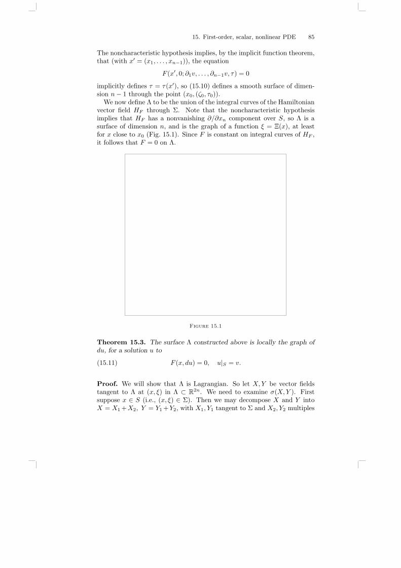
15. First-order, scalar, nonlinear PDE 85
The noncharacteristic hypothesis implies, by the implicit function theorem,that (with x′ = (x1, . . . , xn−1)), the equation
F (x′, 0; ∂1v, . . . , ∂n−1v, τ) = 0
implicitly defines τ = τ(x′), so (15.10) defines a smooth surface of dimen-sion n− 1 through the point (x0, (ζ0, τ0)).
We now define Λ to be the union of the integral curves of the Hamiltonianvector field HF through Σ. Note that the noncharacteristic hypothesisimplies that HF has a nonvanishing ∂/∂xn component over S, so Λ is asurface of dimension n, and is the graph of a function ξ = Ξ(x), at leastfor x close to x0 (Fig. 15.1). Since F is constant on integral curves of HF ,it follows that F = 0 on Λ.
Figure 15.1
Theorem 15.3. The surface Λ constructed above is locally the graph ofdu, for a solution u to
(15.11) F (x, du) = 0, u|S = v.
Proof. We will show that Λ is Lagrangian. So let X,Y be vector fieldstangent to Λ at (x, ξ) in Λ ⊂ R2n. We need to examine σ(X,Y ). Firstsuppose x ∈ S (i.e., (x, ξ) ∈ Σ). Then we may decompose X and Y intoX = X1 +X2, Y = Y1 +Y2, with X1, Y1 tangent to Σ and X2, Y2 multiples
86
of HF at (x, ξ). It suffices to show that σ(X1, Y1) = 0 and σ(X1, Y2) = 0.Since Σ, regarded simply as projecting over xn = 0, is the graph ofa gradient, Proposition 15.2 implies σ(X1, Y1) = 0. On the other hand,σ(X1, Y2) is a multiple of σ(X1,HF ) = 〈X1, dF 〉 = X1F . Since X1 istangent to Σ and F = 0 on Σ, X1F = 0.
Thus we know that σ(X,Y ) = 0 if X and Y are tangent to Λ at a pointin Σ. Suppose now that X and Y are tangent to Λ at a point F t(x, ξ),where (x, ξ) ∈ Σ and F t is the flow generated by HF . We have
σ(X, Y ) =(F t∗σ
)(F t
#X,F t#Y ).
Now F t#X and F t
#Y are tangent to Λ at (x, ξ) ∈ Σ. We use the importantfact that the flow generated by HF leaves the symplectic form invariant toconclude that
σ(X,Y ) = σ(F t#X,F t
#Y ) = 0.
This shows that Λ is Lagrangian.Thus Λ is the graph of du for some smooth u, uniquely determined up
to an additive constant. Pick x0 ∈ S and set u(x0) = v(x0). We see that,on S, ∂u/∂xj = ∂v/∂xj for 1 ≤ j ≤ n− 1, so this forces u|S = v. We haveseen that F = 0 on Λ, so we have solved (15.11).
An important example of an eikonal equation is
(15.12) |dϕ|2 = 1
on a Riemannian manifold, with metric tensor gjk. In local coordinates,(15.12) is
(15.13)∑
j,k
gjk(x)∂ϕ
∂xj
∂ϕ
∂xk= 1,
where, as before, (gjk) is the matrix inverse to (gjk). We want to give ageometrical description of solutions to this equation. Let ϕ be specifiedon a hypersurface S ⊂ M ;ϕ|S = ψ. Assume that |dψ| < 1 on S. Thenthere are two possible sections of T ∗M over S, giving the graphs of dϕ overS. Pick one of then; call it Σ. As we have seen, the graph of dϕ is theflow-out Λ of Σ, via the flow generated by Hf , with f(x, ξ) = (1/2)|ξ|2 =(1/2)
∑gjk(x)ξjξk, that is, via the “geodesic flow” on T ∗M . The projec-
tions onto M of the integral curves of Hf in T ∗M are geodesics on M . Thegeometrical description of ϕ arises from the following result.
Proposition 15.4. The level surfaces of ϕ are orthogonal to the geodesicsthat are the projections on M of the integral curves of Hf through Σ.
Proof. If we consider a point x ∈ M over which Λ is the graph of dϕ,we have (x, ξ) ∈ Λ, ξ = dϕ(x). The assertion of the proposition is that

15. First-order, scalar, nonlinear PDE 87
the metric tensor, inducing an isomorphism T ∗x M ≈ TxM , identifies ξ withγ′(t), where γ′(t), the tangent vector to such a geodesic, is the projectiononto TxM of Hf at (x, ξ). Since
(15.14) Hf =∑[ ∂f
∂ξj
∂
∂xj− ∂f
∂xj
∂
∂ξj
],
this projection is equal to
(15.15)∑ ∂f
∂ξj
∂
∂xj=
∑gjk(x)ξk
∂
∂xj,
which is in fact the image of ξ ∈ T ∗x under the natural metric isomorphismT ∗x M ≈ TxM . This proves the proposition.
We can restate it this way. The metric isomorphism T ∗M ≈ TM pro-duces from the 1-form dϕ, the gradient vector field grad ϕ. In local coor-dinates, with dϕ =
∑(∂ϕ/∂xj) dxj , we have
(15.16) grad ϕ =∑
gjk(x)∂ϕ
∂xj
∂
∂xk.
Thus, the content of the last proposition is the following:
Corollary 15.5. If γ(t) is the geodesic of unit speed that is the projectionon M of an integral curve of Hf through Σ, then
(15.17) grad ϕ(x) = γ′(t), at x = γ(t).
Suppose, for example, that for an initial condition on ϕ we take ϕ = c(constant) on the surface S. Then, near S, the other level sets of ϕ aredescribed as follows. For p ∈ S, let γp(t) be the unit-speed geodesic throughp, so γp(0) = p, orthogonal to S, going in one of two possible directions,corresponding to a choice of one of two possible Σs, as mentioned above.Then
(15.18) ϕ(x) = c + t, at x = γp(t).
This gives a very geometrical picture of solutions to (15.12).On flat Euclidean space, where geodesics are just straight lines, these
formulas become quite explicit. Suppose, for example, that we want tosolve |dϕ|2 = 1 on Rn (i.e.,
∑(∂ϕ/∂xj)2 = 1), and we prescribe
(15.19) ϕ = 0 on a surface S defined by ψ(x) = 0,
where ψ(x) is given. Then it is clear that, for |t| not too large, ϕ is definedby
(15.20) ϕ(x + t|∇ψ(x)|−1∇ψ(x)
)= t, for x ∈ S.
88
For small a, I = (−a, a), the map
(15.21) Ψ : S × I −→ Rn
given by
(15.22) Ψ(x, t) = x + t|∇ψ(x)|−1∇ψ(x)
is a diffeomorphism, but simple examples show that this can break downfor large |t|.
Having solved the special sort of first-order PDE known as the eikonalequation, we now tackle the general case (15.1)–(15.2), subject to the condi-tion (15.3). We use a method, called Jacobi’s trick, of defining u implicitlyby
(15.23) V (x, u(x)) = 0
and producing a PDE for V of the eikonal type. Indeed (15.23) gives, withV = V (x, z),
(15.24) ∇xV + Vz∇u = 0, or ∇u = −V −1z ∇xV,
so set
(15.25) g(x, z, ξ, ζ) = F (x, z,−ζ−1ξ).
Our equation for V is hence F (x, z,−V −1z ∇xV ) = 0, or
(15.26) g(x, z,∇x,zV ) = 0.
This is of eikonal type. Our initial condition is
(15.27) V = z − v on xn = 0.
This gives Vz 6= 0 locally, so by the implicit function theorem, (15.23)defines a function u(x), which solves the system (15.1)–(15.2).
Exercises
1. Let X be a vector field on a region Ω, generating a flow F t, which we willassume is defined everywhere. Consider the linear PDE
(15.28)∂u
∂t= Xu, u(0, x) = f(x).
Show that a solution is given by
u(t, x) = f(F tx).
Show that the equation
(15.29)∂u
∂t= Xu + g(t, x), u(0, x) = f(x)
Exercises 89
is solved by
u(t, x) = f(F tx) +
∫ t
0
g(s,F t−sx
)ds,
and that
(15.30)∂u
∂t= Xu + a(t, x)u, u(0, x) = f(x)
is solved by
u(t, x) = e
(∫ t0 a(s,Ft−sx)ds
)
f(F tx).
(Hint: The solution to (15.28) is constant on integral curves of ∂/∂t − X inR × Ω. Apply Duhamel’s principle to (15.29). Then find A(t, x) such that(15.30) is equivalent to
e−A
(∂
∂t−X
)(eAu
)= 0.)
2. A PDE of the form
∂u
∂t+
n∑j=1
aj(x, u)∂u
∂xj= 0,
for a real-valued u = u(t, x), is a special case of a quasilinear equation. Showthat if we set u(0, x) = v(x) ∈ C∞(Rn), then there is a unique smooth solutionin a neighborhood of 0×Rn in Rn+1, and u(t, x) has the following property.For each x0 ∈ Rn, consider the vector field
Vx0 =∂
∂t+
n∑j=1
aj(x, v(x0))∂
∂xj.
Then u(t, x) is equal to v(x0) on the integral curve of Vx0 through (0, x0).Considering the example
ut + uux = 0, u(0, x) = e−x2,
show that this smooth solution can cease to exist globally, due to two suchlines crossing.
3. Work out explicitly the solution to(
∂ϕ
∂x
)2
+
(∂ϕ
∂y
)2
= 1,
satisfying ϕ(x, y) = 0 on the parabola y = x2, and ∂ϕ/∂y > 0 there, using(15.19) and (15.20). Write a computer program to graph the level curves ofϕ. How does the solution break down?
4. The group of dilations of T ∗M , defined (in local coordinates) by D(r)(x, ξ) =(x, rξ), is generated by a vector field ϑ on T ∗M , which we call the naturalradial vector field. Show that ϑ is uniquely specified by the identity
σ(ϑ, X) = 〈X, κ〉,when X is a vector field on T ∗M , and κ =
∑ξj dxj is the contact form (14.17).
90
5. Suppose Λ is a submanifold of T ∗M of dimension n = dim M , with ι : Λ →T ∗M . Show that Λ is Lagrangian if and only if ι∗κ is a closed 1-form on Λ(hence locally exact). If Λ is Lagrangian, relate ι∗κ = df on Λ to du, in thecontext of Proposition 15.1.
6. Suppose Λ is a Lagrangian submanifold of T ∗M , transverse to ϑ. Define asubbundle V of TΛ by
V(x,ξ) = (ϑ)σ ∩ T(x,ξ)Λ,
where (ϑ)σ is the set of vectors v ∈ T(x,ξ)T∗M such that σ(ϑ, v) = 0. Show
that V is an integrable subbundle of TΛ, that is, that Frobenius’s theoremapplies to V, giving a foliation of Λ. If Λ is the graph of du, u ∈ C∞(M),show that the inverse image, under π : Λ → M , of the level sets of u gives theleaves of this foliation of Λ.
16. Completely integrable Hamiltonian systems
Here we will examine the consequences of having n “conservation laws” fora Hamiltonian system with n degrees of freedom. More precisely, supposeO is a region in R2n, with coordinates (x, ξ) and symplectic form σ =∑n
j=1 dξj ∧ dxj , or more generally O could be a symplectic manifold ofdimension 2n. Suppose we have n functions u1, . . . , un, in involution, thatis,
(16.1) uj , uk = 0, 1 ≤ j, k ≤ n.
The function u1 = F could be the energy function whose Hamiltonian vec-tor field we want to analyze, and u2, . . . , un auxiliary functions, constructedto reflect conservation laws. We give some examples shortly. In case onehas n such functions, with linearly independent gradients, one is said tohave a completely integrable system.
Our goal here will be to show that in such a case the flows generated bythe Huj can be constructed by quadrature. We define the last concept asfollows. Given a collection of functions uj, a map is said to be constructedby quadrature if it is produced by a composition of the following operations:
(i) elementary algebraic manipulation,(ii) differentiation,(iii) integration,(iv) constructing inverses of maps.
To begin the study of a completely integrable system, given (16.1), con-sider, for a given p ∈ Rn, the level set
(16.2) Mp = (x, ξ) ∈ O : uj(x, ξ) = pj.Assuming the uj have linearly independent gradients, each nonempty Mp
is a manifold of dimension n. Note that each vector field Huj is tangent toMp, by (16.1), and therefore Huj : 1 ≤ j ≤ n spans the tangent space to
16. Completely integrable Hamiltonian systems 91
Mp at each point. Since σ(Huj,Huk
) = uj , uk, we conclude from (16.1)that
(16.3) each Mp is Lagrangian.
If we make the “generic” hypothesis
(16.4) π : Mp → Rn is a local diffeomorphism,
where π(x, ξ) = x, then Mp is the graph of a closed 1-form Ξp (dependingsmoothly on p); note that Ξp(x) is constructed by inverting a map, one ofthe operations involved in construction by quadrature. Furthermore, Ξp
being closed, we can construct a smooth function ϕ(x, p) such that
(16.5) Mp is the graph of x 7→ dxϕ(x, p).
The function ϕ(x, p) is constructed from Ξp by an integration, anotheringredient in construction by quadrature. Note that a statement equivalentto (16.5) is that ϕ simultaneously satisfies the eikonal equations
(16.6) uj
(x, dxϕ(x, p)
)= pj , 1 ≤ j ≤ n.
Consider now the following maps:
(16.7)
(x, p) F1−−−−→ (dpϕ(x, p), p
)
Cy
(x, p) F2−−−−→ (x, dxϕ(x, p)
).
Since F2(x, p) = (x,Ξp(x)), it is clear that F2 is a local diffeomorphismunder our hypotheses. This implies that the matrix
(16.8)∂2ϕ
∂pj∂xk
is invertible, which hence implies that F1 is a local diffeomorphism (by theinverse function theorem). Hence C is locally defined, as a diffeomorphism:
(16.9) C(dpϕ(x, p), p)
=(x, dxϕ(x, p)
).
Write C(q, p) = (x, ξ). Note that
(16.10)F ∗2
∑dξj ∧ dxj =
∑
j,k
∂2ϕ
∂pk∂xjdpk ∧ dxj
= F ∗1∑
dpj ∧ dqj ,
so
(16.11) C∗(∑
dξj ∧ dxj
)=
∑dpj ∧ dqj ,
that is, C preserves the symplectic form. One says C is a canonical trans-formation with generating function ϕ(x, p). Now conjugation by C takes
92
the Hamiltonian vector fields Hujon (x, ξ)-space to the Hamiltonian vector
fields Hujon (q, p)-space, with
uj(q, p) = uj C(q, p) = pj ,
in view of (16.6). Thus
(16.12) Huj =∂
∂qj,
so C conjugates the flows generated by Huj to simple straight-line flows.This provides the construction of the Huj
-flows by quadrature.Note that if O has dimension 2, one needs only one function u1. Thus
the construction above generalizes the treatment of Hamiltonian systemson R2 given in §10. In fact, the approach given above, specialized to n = 1,is closer to the analysis in §10 than it might at first appear. Using notationas in §10, let u1 = f, p1 = E, so
ME = (x, ξ) : f(x, ξ) = Eis the graph of ξ = ψ(x, E) = dxϕ(x,E), with
ϕ(x,E) =∫
ψ(x,E) dx.
Note that f(x, ψ(x,E)) = E ⇒ fξψE = 1, so
(16.13) dEϕ(x, E) =∫
fξ
(x, ψ(x,E)
)−1dx,
and C maps (∫
f−1ξ dx,E) to (x, ψ(x, ξ)). To say C conjugates Hf to HE =
∂/∂q (in (q, E) coordinates) is to say that under the time-t Hamiltonianflow,
∫f−1
ξ dx is augmented by t; but this is precisely the content of (10.16),namely,
(16.14)∫
fξ
(x, ψ(x, E)
)−1dx = t + C(E).
We also note that, for the purpose of linearizing Hu1 , it suffices to haveϕ(x, p), satisfying only the eikonal equation
(16.15) u1
(x, dxϕ(x, p)
)= p1,
such that the matrix (16.8) is invertible. The existence of u2, . . . , un, whichtogether with u1 are in involution, provides a way to construct ϕ(x, p), butany other successful attack on (16.15) is just as satisfactory. IntegratingHu1 by perceiving solutions to (16.15) is the essence of the Hamilton-Jacobimethod.
We now look at some examples of completely integrable Hamiltoniansystems. First we consider geodesic flow on a two-dimensional surface ofrevolution M2 ⊂ R3. Note that T ∗M2 is four-dimensional, so we wantu1 and u2, in involution. The function u1 is, of course, the energy funtion
16. Completely integrable Hamiltonian systems 93
u1 = (1/2)∑
gjk(x)ξjξk; as we have seen, Hu1 generates the geodesicflow. Our function u2 will arise from the group of rotations Rθ of M2
about its axis of symmetry, θ ∈ R/2πZ. This produces a group Rθ ofcanonical transformations of T ∗M2, generated by a Hamiltonian vectorfield X = Hu2 , with u2(x, ξ) = 〈∂/∂θ, ξ〉. Since Rθ is a group of isometriesof M2, Rθ preserves u1 (i.e., Xu1 = 0), or equivalently, u2, u1 = 0. Wehave our pair of functions in involution. Thus geodesics on such a surfaceof revolution can be constructed by quadrature.
Another important class of completely integrable Hamiltonian systemsis provided by motion in a central force field in the plane R2. In otherwords, let x(t), a path in R2, satisfy
(16.16) x = −∇V (x), V (x) = v(|x|).The Hamiltonian system is
(16.17) x = ∇ξF, ξ = −∇xF,
with
(16.18) F (x, ξ) =12|ξ|2 + v(|x|).
We take u1 = F and look for u2, in involution. Again u2 arises from agroup of rotations, this time rotations of R2 about the origin. The methodwe have given by which a vector field on Ω produces a Hamiltonian vectorfield on T ∗Ω yields the formula
(16.19)
u2(x, ξ) =⟨ ∂
∂θ, ξ
⟩
=⟨−x2
∂
∂x1+ x1
∂
∂x2, ξ
⟩
= x1ξ2 − x2ξ1.
This is the “angular momentum.” The symmetry of V (x) implies thatthe group of rotations on T ∗R2 generated by Hu2 preserves F = u1, thatis,
(16.20) u1, u2 = 0,
a fact that is also easily verified from (16.18) and (16.19) by a computation.This expresses the well-known law of conservation of angular momentum.It also establishes the complete integrability of the general central forceproblem on R2. We remark that, for the general central force problem inRn, conservation of angular momentum forces any path to lie in a plane,so there is no loss of generality in studying planar motion.
The case
(16.21) V (x) = −K
|x| (K > 0)
94
of the central force problem is called the Kepler problem. It gives Newton’sdescription of a planet traveling about a massive star, or of two celestialbodies revolving about their center of mass. We will give a direct study ofcentral force problems, with particular attention to the Kepler problem, inthe next section.
These examples of completely integrable systems have been based ononly the simplest of symmetry considerations. For many other examples ofcompletely integrable systems, see [Wh].
We have dealt here only with the local behavior of completely integrablesystems. There is also an interesting “global” theory, which among otherthings studies the distinction between the regular behavior of completelyintegable systems on the one hand and varieties of “chaotic behavior” ex-hibited by (globally) nonintegrable systems on the other. The reader canfind out more about this important topic (begun in [Poi]) in [Mos], [TS],[Wig], and references given therein.
Exercises
1. Let u1(x, ξ) = (1/2)|ξ|2−|x|−1 be the energy function for the Kepler problem(with K = 1), and let u2(x, ξ) be given by (16.19). Set
vj(x, ξ) = xj |x|−1 − xj |ξ|2 + (x · ξ)ξj , j = 1, 2.
(v1, v2) is called the Lenz vector. Show that the following Poisson bracketrelations hold:
u1, vj = 0, j = 1, 2,
u2, vj = ±vj ,
v1, v2 = 2u1u2.
Also show that
v21 + v2
2 − 2u1u22 = 1.
2. Deduce that the Kepler problem is integrable in several different ways. Canyou relate this to the fact that all bounded orbits are periodic?
In Exercises 3–5, suppose a given Mp, as in (16.2), is compact, and duj , 1 ≤j ≤ n are linearly independent at each point of Mp.
3. Show that there is an Rn-action on Mp, defined by Φ(t)(ζ) = F t11 · · · F tn
n ζ, fort = (t1, . . . , tn), ζ ∈ Mp, where Fs
j is the flow generated by Huj . Show thatΦ(t + s)ζ = Φ(t)Φ(s)ζ.
4. Show that Rn acts transitively on Mp, that is, given ζ ∈ Mp, O(ζ) = Φ(t)ζ :t ∈ Rn is all of Mp. (Hint: Use the linear independence to show O(ζ) is open.Then, if ζ1 is on the boundary of O(ζ) in Mp, show that O(ζ1) ∩ O(ζ) 6= ∅.)
5. Fix ζ0 ∈ Mp and let Γ = t ∈ Rn : Φ(t)ζ0 = ζ0. Show that Mp is diffeomor-phic to Rn/Γ and that this is a torus.
6. If u1 = F can be extended to a completely integrable system in two differentways, with the setting of Exercises 3–5 applicable in each case, then phase
17. Examples of integrable systems; central force problems 95
space may be foliated by tori in two different ways. Hence intersections ofvarious tori will be invariant under HF . How does this relate to Exercise 2?
17. Examples of integrable systems; central force problems
In the last section it was noted that central force problems give rise toa class of completely integrable Hamiltonian systems with two degrees offreedom. Here we will look at this again, from a more elementary point ofview. We look at a class of Hamiltonians on a region in R4, of the form
(17.1) F (y, η) = F (y1, η1, η2),
that is, with no y2-dependence. Thus Hamilton’s equations take the form
(17.2) yj =∂F
∂ηj, η1 = − ∂F
∂y1, η2 = 0.
In particular, η2 is constant on any orbit, say
(17.3) η2 = L.
This, in addition to F , provides the second conservation law implying in-tegrability; note that F, η2 = 0. If F (y1, η1, L) = E on an integral curve,we write this relation as
(17.4) η1 = ψ(y1, L,E).
We can now pursue an analysis that is a variant of that described by(10.14)–(10.20). The first equation in (17.2) becomes
(17.5) y1 = Fη1
(y1, ψ(y1, L,E), L
),
with solution given implicitly by
(17.6)∫
Fη1
(y1, ψ(y1, L, E), L
)−1dy1 = t + C.
Once one has y1(t), then one has
(17.7) η1(t) = ψ(y1(t), L, E),
and then the remaining equation in (17.2) becomes
(17.8) y2 = Fη2
(y1(t), η1(t), L
),
which is solved by an integration.We apply this method to the central force problem, with
(17.9) F (x, ξ) =12|ξ|2 + v(|x|), x ∈ R2.
Use of polar coordinates is clearly suggested, so we set
(17.10) y1 = r, y2 = θ; x1 = r cos θ, x2 = r sin θ.
96
In these coordinates, the Euclidean metric dx21 + dx2
2 becomes dr2 + r2dθ2,so, as in (12.31), the function F becomes
(17.11) F (y, η) =12(η21 + y−2
1 η22
)+ v(y1).
We see that the first pair of ODEs in (17.2) takes the form
(17.12) r = η1, θ = Lr−2,
where L is the constant value of η2 along an integral curve, as in (17.3).The last equation, rewritten as
(17.13) r2θ = L,
expresses conservation of angular momentum. The remaining ODE in(17.2) becomes
(17.14) η1 = L2r−3 − v′(r).
Note that differentiating the first equation of (17.12) and using (17.14)gives
(17.15) r = L2r−3 − v′(r),
an equation that can be integrated by the methods described in (10.12)–(10.20). We will not solve (17.15) by this means here, though (17.15) willbe used below, to produce (17.23). For now, we instead use (17.4)–(17.6).In the present case, (17.4) takes the form
(17.16) η1 = ±[2E − 2v(r)− L2r−2
]1/2,
and since Fη1 = η1, (17.6) takes the form
(17.17) ±∫ [
2Er2 − 2r2v(r)− L2]−1/2
r dr = t + C.
In the case of the Kepler problem (16.21), where v(r) = −K/r, the resultingintegral
(17.18) ±∫ (
2Er2 + 2Kr − L2)−1/2
r dr = t + C
can be evaluated using techniques of first-year calculus, by completing thesquare in 2Er2 + 2Kr − L2. Once r = r(t) is given, the equation (17.13)provides an integral formula for θ = θ(t).
One of the most remarkable aspects of the analysis of the Kepler problemis the demonstration that orbits all lie on some conic section, given in polarcoordinates by
(17.19) r[1 + e cos(θ − θ0)
]= ed,
where e is the “eccentricity.” We now describe the famous, elementary butingenious trick used to demonstrate this. The method involves producing
Exercises 97
a differential equation for r in terms of θ, from (17.13) and (17.15). Moreprecisely, we produce a differential equation for u, defined by
(17.20) u = r−1.
By the chain rule,
(17.21)dr
dt= −r2 du
dt= −r2 du
dθ
dθ
dt= −L
du
dθ,
in light of (17.13). Differentiating this with respect to t gives
(17.22)d2r
dt2= −L
d
dt
du
dθ= −L
d2u
dθ2
dθ
dt= −L2u2 d2u
dθ2,
again using (17.13). Comparing this with (17.15), we get−L2u2(d2u/dθ2) =L2u3 − v′(1/u) or, equivalently,
(17.23)d2u
dθ2+ u = (Lu)−2v′
( 1u
).
In the case of the Kepler problem, v(r) = −K/r, the right side becomesthe constant K/L2, so in this case (17.23) becomes the linear equation
(17.24)d2u
dθ2+ u =
K
L2,
with general solution
(17.25) u(θ) = A cos(θ − θ0) +K
L2,
which is equivalent to the formula (17.19) for a conic section.For more general central force problems, the equation (17.23) is typically
not linear, but it is of the form treatable by the method of (10.12)–(10.20).
Exercises
1. Solve explicitly w′′(t) = −w(t), for w taking values in R2 = C. Show that|w(t)|2 + |w′(t)|2 = 2E is constant for each orbit.
2. For w(t) taking values in C, define a new curve by
Z(τ) = w(t)2,dτ
dt= |w(t)|2.
Show that if w′′(t) = −w(t), then
Z′′(τ) = −4EZ(τ)
|Z(τ)|3 ,
that is, Z(τ) solves the Kepler problem.3. Analyze the flow of HF , for F of the form (17.1), in a manner more directly
parallel to the approach in §16, in a spirit similar to (16.13) and (16.14). Note
98
that, with u1 = F, u2 = η2, p1 = E, p2 = L, the canonical transformation Cof (16.9) is defined by
C(∫
F−1η1 dy1, y2 −
∫F−1
η1 Fη2 dy1; E, L
)=
(y1, y2; ψ(y1, L, E), L
),
where the first integrand is Fη1
(y1, ψ(y1, L, E), L
)−1
, and so on.
4. Analyze the equation (17.23) for u(θ) in the following cases.
(a) v(r) = −K/r2,(b) v(r) = Kr2,(c) v(r) = −K/r + εr2.
Show that, in case (c), u(θ) is typically not periodic in θ.5. Consider motion on a surface of revolution, under a force arising from a ro-
tationally invariant potential. Show that you can choose coordinates (r, θ) sothat the metric tensor is ds2 = dr2 + β(r)−1 dθ2, and then you get a Hamil-tonian system of the form (17.2) with
F (y1, η1, η2) =1
2η21 +
1
2β(y1)η
22 + v(y1),
where y1 = r, y2 = θ. Show that, parallel to (17.16) and (17.17), you get
r = ±[2E − 2v(r)− L2β(r)
]1/2
.
Show that u = 1/r satisfies
du
dθ= ∓ u2
Lβ(1/u)
[2E − 2v
(1
u
)− L2β
(1
u
)]1/2
.
18. Relativistic motion
Mechanical systems considered in previous sections were formulated in theNewtonian framework. The description of a particle moving subject to aforce was given in terms of a curve in space (with a positive-definite metric),parameterized by time. In the relativistic set-up, one has not space andtime as separate entities, but rather spacetime, provided with a metric ofLorentz signature. In particular, Minkowski spacetime is R4 with innerproduct
(18.1) 〈x, y〉 = −x0y0 +3∑
j=1
xjyj ,
given x = (x0, . . . , x3), y = (y0, . . . , y3). The behavior of a particle movingin a force field is described by a curve in spacetime, which is timelike, thatis, its tangent vector T satisfies 〈T, T 〉 < 0. We parameterize the curve notby time, but by arc length, so we consider a curve x(τ) satisfying
(18.2) 〈u(τ), u(τ)〉 = −1, u(τ) = x′(τ).
18. Relativistic motion 99
The parameter τ is often called “proper time,” and u(τ) the “4-velocity.”Such a curve x(τ) is sometimes called a “world line.”
Relativistic laws of physics are to be formulated in a manner dependingonly on the Lorentz metric (18.1), but contact is made with the Newtonianpicture by using the product decomposition R4 = R × R3, writing x =(t, xs), t = x0, and xs = (x1, x2, x3). The “3-velocity” is v = dxs/dt. Then
(18.3) u = γ(1, v),
where, by (18.2),
(18.4) γ =dt
dτ=
(1− |v|2)−1/2
,
with |v|2 = v21 + v2
2 + v23 . In the limit of small velocities, γ is close to 1.
The particle whose motion is to be described is assumed to have a con-stant “rest mass” m0, and then the “4-momentum” is defined to be
(18.5) p = m0u.
In terms of the decomposition (18.3),
(18.6) p = (m0γ,m0γv),
where m0v is the momentum in Newtonian theory. The replacement forNewton’s equation m0dv/dt = f is
(18.7)dp
dτ= F,
the right side being the “Minkowski 4-force.”Newtonian theory and Einstein’s relativity are related as follows. Define
m by m = m0γ and, using (18.6) and (18.7), write
(18.8) F =(dm
dτ,d(mv)
dτ
)=
(dm
dτ, γ
d(mv)dt
).
Then we identify fC = d(mv)/dt as the “classical force” and write the lastexpression as (f0, γfC). If (18.2) is to hold, we require f0 = γfC · v (thedot product in Euclidean R3), so
(18.9) F = γ(fC · v, fC).
With this correspondence, the equation (18.7) yields Newton’s equation inthe small velocity limit.
Since the 4-velocity has constant length, by (18.2), the Minkowski 4-forceF must satisfy
(18.10) 〈F, u〉 = 0.
It follows that in relativity one cannot have velocity-independent forces.The simplest situation compatible with (18.10) is for F to be linear in u,say
(18.11) F (x, u) = F(x)u,
100
where for each x ∈ R4, F(x) is a linear transformation on R4; in otherwords, F is a tensor field of type (1, 1). The condition (18.10) holds pro-vided F is skew-adjoint with respect to the Lorentz inner product:
(18.12) 〈Fu, w〉 = −〈u, Fw〉.Equivalently, if we consider the related tensor F of type (0, 2),
(18.13) F(u,w) = 〈u, Fw〉,then F is antisymmetric, that is, F is a 2-form. In index notation, Fjk =hj`F`
k, where hjk defines the Lorentz metric.The electromagnetic field is of this sort. The classical force exerted by
an electric field E and a magnetic field B on a particle with charge e is theLorentz force
(18.14) fL = e(E + v ×B),
as in (12.40). Using this in (18.9) gives, for u = (u0, v),
(18.15) Fu = e(E · v,Eu0 + v ×B).
Consequently the 2-form F is F(u, w) = e∑Fµνuµwν with
(18.16)(Fµν
)=
0 −E1 −E2 −E3
E1 0 B3 −B2
E2 −B3 0 B1
E3 B2 −B1 0
.
In relativity it is this 2-form which is called the electromagnetic field.To change notation slightly, let us denote by F the 2-form described by
(18.16), namely, with t = x0,
(18.17) F =3∑
j=1
Ej dxj ∧ dt+B1 dx2 ∧ dx3 +B2 dx3 ∧ dx1 +B3 dx1 ∧ dx2.
Thus the force in (18.11) is now denoted by eFu.We can construct a Lagrangian giving the equation of motion (18.7),
(18.11), in a fashion similar to (12.44). The part of Maxwell’s equations forthe electromagnetic field recorded as (12.41) is equivalent to the statementthat
(18.18) dF = 0.
Thus we can find a 1-form A on Minkowski spacetime such that
(18.19) F = dA.
Then we can set
(18.20) L(x, u) =12m0〈u, u〉+ e〈A, u〉,
Exercises 101
and the force law dp/dτ = eF(x)u is seen to be equivalent to
(18.21)d
dτLu − Lx = 0.
See Exercise 3 below. In this case, the Legendre transform (12.13) becomes,with ub = (−u0, u1, u2, u3),
(18.22) (x, ξ) = (x,m0ub + eA),
and we get the Hamiltonian system
(18.23)dx
dτ= Eξ,
dξ
dτ= −Ex,
with
(18.24) E(x, ξ) =1
2m0
⟨ξ − eA, ξ − eA⟩
.
Exercises
1. Consider a constant electromagnetic field of the form
E = (1, 0, 0), B = 0.
Work out the solution to Newton’s equation
mdv
dt= e(E + v ×B), v =
dx
dt,
for the path x = x(t) in R3 of a particle of charge e, mass m, moved bythe Lorentz force arising from this field. Then work out the solution to therelativistic equation
m0du
dτ= e(E · v, Eu0 + v ×B),
with u = (u0, v) (having square norm −1), u = dx/dτ , for the path in R4 ofa particle of charge e, rest mass m0, moved by such an electromagnetic field.Compare the results. Do the same for
E = 0, B = (1, 0, 0).
2. Take another look at Exercise 3 in §12.3. Show that taking (18.20) for the Lagrangian implies that Lagrange’s equation
(18.21) is equivalent to the force law dp/dτ = eFu, on Minkowski spacetime.(Hint: To compute Lx, use
d〈A, u〉 = −(dA)cu + LuA,
regard u as independent of x, and note that dA/dτ = ∇uA = LuA, in thatcase.)Compare Exercise 4 in §12.
4. Verify formula (18.16) for Fµν . Show that the matrix for F has the sameform, except all Ej carry plus signs.

102
5. An alternative sign convention for the Lorentz metric on Minkowski spacetimeis to replace (18.1) by 〈x, y〉 = x0y0 −
∑j≥1 xjyj . Show that this leads to a
sign change in (18.16). What other sign changes arise?6. Suppose a 1-form A is given, satisfying (18.19), on a general four-dimensional
Lorentz manifold M . Let L : TM → R be given by (18.20). Use the set-up described in (12.51)–(12.65) to derive equations of motion, extending theLorentz force law from Minkowski spacetime to any Lorentz 4-manifold.(Hint: In analogy with (12.64), show that Lv is given by
Lv = m0u + eA#,
where A# is the vector field corresponding to A via the metric (by raisingindices). Taking a cue from Exercise 3, show that Lx satisfies
Lx = eFu + e∇uA#.
Deduce that the equation
m0∇uu = eFu
is the stationary condition for this Lagrangian.)
19. Topological applications of differential forms
Differential forms are a fundamental tool in calculus. In addition, theyhave important applications to topology. We give a few here, starting withsimple proofs of some important topological results of Brouwer.
Proposition 19.1. There is no continuous retraction ϕ : B → Sn−1 ofthe closed unit ball B in Rn onto its boundary Sn−1.
In fact, it is just as easy to prove the following more general result. Theapproach we use is adapted from [Kan].
Proposition 19.2. If M is a compact, oriented manifold with nonemptyboundary ∂M , there is no continuous retraction ϕ : M → ∂M .
Proof. A retraction ϕ satisfies ϕ j(x) = x, where j : ∂M → M is thenatural inclusion. By a simple approximation, if there were a continuousretraction there would be a smooth one, so we can suppose ϕ is smooth.
Pick ω ∈ Λn−1(∂M) to be the volume form on ∂M , endowed with someRiemannian metric (n = dim M), so
∫∂M
ω > 0. Now apply Stokes’theorem to α = ϕ∗ω. If ϕ is a retraction, j∗ϕ∗ω = ω, so we have
(19.1)∫
∂M
ω =∫
M
dϕ∗ω.
But dϕ∗ω = ϕ∗dω = 0, so the integral (19.1) is zero. This is a contradiction,so there can be no retraction.
19. Topological applications of differential forms 103
A simple consequence of this is the famous Brouwer fixed-point theorem.
Theorem 19.3. If F : B → B is a continuous map on the closed unit ballin Rn, then F has a fixed point.
Proof. We are claiming that F (x) = x for some x ∈ B. If not, defineϕ(x) to be the endpoint of the ray from F (x) to x, continued until ithits ∂B = Sn−1. It is clear that ϕ would be a retraction, contradictingProposition 19.1.
We next show that an even-dimensional sphere cannot have a smoothnonvanishing vector field.
Proposition 19.4. There is no smooth nonvanishing vector field on Sn ifn = 2k is even.
Proof. If X were such a vector field, we could arrange it to have unitlength, so we would have X : Sn → Sn, with X(v) ⊥ v for v ∈ Sn ⊂ Rn+1.Thus there is a unique unit-speed geodesic γv from v to X(v), of lengthπ/2. Define a smooth family of maps Ft : Sn → Sn by Ft(v) = γv(t). ThusF0(v) = v, Fπ/2(v) = X(v), and Fπ = A would be the antipodal map,A(v) = −v. By (13.63), we deduce that A∗ω− ω = dβ is exact, where ω isthe volume form on Sn. Hence, by Stokes’ theorem,
(19.2)∫
Sn
A∗ω =∫
Sn
ω.
On the other hand, it is straightforward that A∗ω = (−1)n+1ω, so (19.2)is possible only when n is odd.
Note that an important ingredient in the proof of both Proposition 19.2and Proposition 19.4 is the existence of n-forms on a compact, oriented,n-dimensional manifold M which are not exact (though of course they areclosed). We next establish the following important counterpoint to thePoincare lemma.
Proposition 19.5. If M is a compact, connected, oriented manifold ofdimension n and α ∈ ΛnM , then α = dβ for some β ∈ Λn−1(M) if andonly if
(19.3)∫
M
α = 0.
We have already discussed the necessity of (19.3). To prove the suffi-ciency, we first look at the case M = Sn.
104
In that case, any n-form α is of the form a(x)ω, a ∈ C∞(Sn), ω thevolume form on Sn, with its standard metric. The group G = SO(n + 1)of rotations of Rn+1 acts as a transitive group of isometries on Sn. InAppendix B, Manifolds, Vector Bundles, and Lie Groups, we construct theintegral of functions over SO(n + 1), with respect to Haar measure.
As noted in Appendix B, we have the map Exp : Skew(n+1) → SO(n+1), giving a diffeomorphism from a ball O about 0 in Skew(n + 1) onto anopen set U ⊂ SO(n + 1) = G, a neighborhood of the identity. Since Gis compact, we can pick a finite number of elements ξj ∈ G such that theopen sets Uj = ξjg : g ∈ U cover G. Pick ηj ∈ Skew(n + 1) such thatExp ηj = ξj . Define Φjt : Uj → G for 0 ≤ t ≤ 1 by
(19.4) Φjt
(ξj Exp(A)
)= (Exp tηj)(Exp tA), A ∈ O.
Now partition G into subsets Ωj , each of whose boundaries has contentzero, such that Ωj ⊂ Uj . If g ∈ Ωj , set g(t) = Φjt(g). This family ofelements of SO(n + 1) defines a family of maps Fgt : Sn → Sn. Now, as in(13.60), we have
(19.5) α = g∗α− dκg(α), κg(α) =∫ 1
0
F ∗gt(αcXgt) dt,
for each g ∈ SO(n + 1), where Xgt is the family of vector fields on Sn
generated by Fgt, as in (13.58). Therefore,
(19.6) α =∫
G
g∗α dg − d
∫
G
κg(α) dg.
Now the first term on the right is equal to αω, where α =∫
a(g · x)dg is aconstant; in fact, the constant is
(19.7) α =1
Vol Sn
∫
Sn
α.
Thus, in this case, (19.3) is precisely what serves to make (19.6) a repre-sentation of α as an exact form. This finishes the case M = Sn.
For a general compact, oriented, connected M , proceed as follows. CoverM with open sets O1, . . . ,OK such that each Oj is diffeomorphic to theclosed unit ball in Rn. Set U1 = O1, and inductively enlarge each Oj
to Uj , so that U j is also diffeomorphic to the closed ball, and such thatUj+1 ∩ Uj 6= ∅, 1 ≤ j < K. You can do this by drawing a simple curvefrom Oj+1 to a point in Uj and thickening it. Pick a smooth partition ofunity ϕj , subordinate to this cover.
Given α ∈ ΛnM , satisfying (19.3), take αj = ϕjα. Most likely∫
α1 =c1 6= 0, so take σ1 ∈ ΛnM , with compact support in U1 ∩ U2, such that∫
σ1 = c1. Set α1 = α1 − σ1, and redefine α2 to be the old α2 plus σ1.Make a similar construction using
∫α2 = c2, and continue. When you are
19. Topological applications of differential forms 105
done, you have
(19.8) α = α1 + · · ·+ αK ,
with αj compactly supported in Uj . By construction,
(19.9)∫
αj = 0,
for 1 ≤ j < K. But then (19.3) implies∫
αK = 0 too.Now pick p ∈ Sn and define smooth maps
(19.10) ψj : M −→ Sn,
which map Uj diffeomorphically onto Sn \p and map M \Uj to p. There isa unique vj ∈ ΛnSn, with compact support in Sn \ p, such that ψ∗vj = αj .Clearly
∫
Sn
vj = 0,
so by the case M = Sn of Proposition 19.5 already established, we knowthat vj = dwj for some wj ∈ Λn−1Sn, and then
(19.11) αj = dβj , βj = ψ∗j wj .
This concludes the proof.We can sharpen and extend some of the topological results given above,
using the notion of the degree of a map between compact, oriented surfaces.Let X and Y be compact, oriented, n-dimensional surfaces. We want todefine the degree of a smooth map F : X → Y . To do this, assume Y isconnected. We pick ω ∈ ΛnY such that
(19.12)∫
Y
ω = 1.
We want to define
(19.13) Deg(F ) =∫
X
F ∗ω.
The following result shows that Deg(F ) is indeed well defined by this for-mula. The key argument is an application of Proposition 19.5.
Lemma 19.6. The quantity (19.13) is independent of the choice of ω, aslong as (19.12) holds.
Proof. Pick ω1 ∈ ΛnY satisfying∫
Yω1 = 1, so
∫Y
ω − ω1 = 0. ByProposition 19.5, this implies
(19.14) ω − ω1 = dα, for some α ∈ Λn−1Y.
106
Thus
(19.15)∫
X
F ∗ω −∫
X
F ∗ω1 =∫
X
dF ∗α = 0,
and the lemma is proved.
The following is a most basic property.
Proposition 19.7. If F0 and F1 are homotopic, then Deg(F0) = Deg(F1).
Proof. As noted in Exercise 7 of §13, if F0 and F1 are homotopic, thenF ∗0 ω − F ∗1 ω is exact, say dβ, and of course
∫X
dβ = 0.
We next give an alternative formula for the degree of a map, which is veryuseful in many applications. A point y0 ∈ Y is called a regular value of Fprovided that, for each x ∈ X satisfying F (x) = y0, DF (x) : TxX → Ty0Yis an isomorphism. The easy case of Sard’s theorem, discussed in AppendixB, implies that most points in Y are regular. Endow X with a volumeelement ωX , and similarly endow Y with ωY . If DF (x) is invertible, defineJF (x) ∈ R \ 0 by F ∗(ωY ) = JF (x)ωX . Clearly the sign of JF (x) (i.e., sgnJF (x) = ±1), is independent of the choices of ωX and ωY , as long as theydetermine the given orientations of X and Y .
Proposition 19.8. If y0 is a regular value of F , then
(19.16) Deg(F ) =∑
sgn JF (xj) : F (xj) = y0.
Proof. Pick ω ∈ ΛnY , satisfying (19.12), with support in a small neigh-borhood of y0. Then F ∗ω will be a sum
∑ωj , with ωj supported in a small
neighborhood of xj , and∫
ωj = ±1 as sgn JF (xj) = ±1.
The following result is a powerful tool in degree theory.
Proposition 19.9. Let M be a compact, oriented manifold with bound-ary. Assume that dim M = n + 1. Given a smooth map F : M → Y , letf = F
∣∣∂M
: ∂M → Y . Then
Deg(f) = 0.
Proof. Applying Stokes’ theorem to α = F ∗ω, we have∫
∂M
f∗ω =∫
M
dF ∗ω.
But dF ∗ω = F ∗dω, and dω = 0 if dim Y = n, so we are done.

19. Topological applications of differential forms 107
An easy corollary of this is another proof of Brouwer’s no-retractiontheorem. Compare the proof of Proposition 19.2.
Corollary 19.10. If M is a compact, oriented manifold with nonemptyboundary ∂M , then there is no smooth retraction ϕ : M → ∂M .
Proof. Without loss of generality, we can assume that M is connected.If there were a retraction, then ∂M = ϕ(M) must also be connected, soProposition 19.9 applies. But then we would have, for the map id. = ϕ
∣∣∂M
,the contradiction that its degree is both 0 and 1.
For another application of degree theory, let X be a compact, smooth,oriented hypersurface in Rn+1, and set Ω = Rn+1 \ X. (Assume n ≥ 1.)Given p ∈ Ω, define
(19.17) Fp : X −→ Sn, Fp(x) =x− p
|x− p| .
It is clear that Deg(Fp) is constant on each connected component of Ω. Itis also easy to see that, when p crosses X, Deg(Fp) jumps by ±1. Thus Ωhas at least two connected components. This is most of the smooth case ofthe Jordan-Brouwer separation theorem:
Theorem 19.11. If X is a smooth, compact, oriented hypersurface ofRn+1, which is connected, then Ω = Rn+1 \X has exactly two connectedcomponents.
Proof. Since X is oriented, it has a smooth, global, normal vector field.Use this to separate a small collar neighborhood C of X into two pieces;C \X = C0 ∪ C1. The collar C is diffeomorphic to [−1, 1]×X, and each Cj
is clearly connected. It suffices to show that any connected component Oof Ω intersects either C0 or C1. Take p ∈ ∂O. If p /∈ X, then p ∈ Ω, whichis open, so p cannot be a boundary point of any component of Ω. Thus∂O ⊂ X, so O must intersect a Cj . This completes the proof.
Let us note that, of the two components of Ω, exactly one is unbounded,say Ω0, and the other is bounded; call it Ω1. Then we claim that if X isgiven the orientation it gets as ∂Ω1,
(19.18) p ∈ Ωj =⇒ Deg(Fp) = j.
Indeed, for p very far from X, Fp : X → Sn is not onto, so its degree is 0.And when p crosses X, from Ω0 to Ω1, the degree jumps by +1.
For a simple closed curve in R2, this result is the smooth case of theJordan curve theorem. That special case of the argument given above canbe found in [Sto].
108
We remark that, with a bit more work, one can show that any compact,smooth hypersurface in Rn+1 is orientable. For one proof, see Appendix Bto Chapter 5.
The next application of degree theory is useful in the study of closedorbits of planar vector fields. Let C be a simple, smooth, closed curvein R2, parameterized by arc length, of total length L. Say C is givenby x = γ(t), γ(t + L) = γ(t). Then we have a unit tangent field toC, T (γ(t)) = γ′(t), defining
(19.19) T : C −→ S1.
Proposition 19.12. For T given by (19.19), we have
(19.20) Deg(T ) = 1.
Proof. Pick a tangent line ` to C such that C lies on one side of `, asin Fig. 19.1. Without changing Deg(T ), you can flatten out C a little, soit intersects ` along a line segment, from γ(L0) to γ(L) = γ(0), where wetake L0 = L− 2ε, L1 = L− ε.
Now T is close to the map Ts : C → S1, given by
(19.21) Ts
(γ(t)
)=
γ(t + s)− γ(t)|γ(t + s)− γ(t)| ,
for any s > 0 small enough; hence T and Ts are homotopic, for smallpositive s. It follows that T and Ts are homotopic for all s ∈ (0, L).Furthermore, we can even let s = s(t) be any continuous function s :[0, L] → (0, L) such that s(0) = s(L). In particular, T is homotopic to themap V : C → S1, obtained from (19.21) by taking
s(t) = L1 − t, for t ∈ [0, L0],
and s(t) going monotonically from L1−L0 to L1, for t ∈ [L0, L]. Note that
V(γ(t)
)=
γ(L1)− γ(t)|γ(L1)− γ(t)| , 0 ≤ t ≤ L0.
The parts of V over the ranges 0 ≤ t ≤ L0 and L0 ≤ t ≤ L, respectively,are illustrated in Figures 19.1 and 19.2. We see that V maps the segmentof C from γ(0) to γ(L0) into the lower half of the circle S1, and it mapsthe segment of C from γ(L0) to γ(L) into the upper half of the circle S1.Therefore, V (hence T ) is homotopic to a one-to-one map of C onto S1,preserving orientation, and (19.20) is proved.
The material of this section can be cast in the language of deRhamcohomology, which we now define. Let M be a smooth manifold. A smoothk-form u is said to be exact if u = dv for some smooth (k− 1)-form v, andclosed if du = 0. Since d2 = 0, every exact form is closed:
(19.22) Ek(M) ⊂ Ck(M),
19. Topological applications of differential forms 109
Figure 19.1
Figure 19.2
where Ek(M) and Ck(M) denote respectively the spaces of exact and closedk-forms. The deRham cohomology groups are defined as quotient spaces:
(19.23) Hk(M) = Ck(M)/Ek(M).
There are no nonzero (−1)-forms, so E0(M) = 0. A 0-form is a real-valuedfunction, and it is closed if and only if it is constant on each connectedcomponent of M , so
(19.24) H0(M) ≈ Rν , ν = # connected components of M.
An immediate consequence of Proposition 19.5 is the following:
110
Proposition 19.13. If M is a compact, connected, oriented manifold ofdimension n, then
(19.25) Hn(M) ≈ R.
Via the pull-back of forms, a smooth map F : X → Y between twomanifolds induces maps on cohomology:
(19.26) F ∗ : Hj(Y ) −→ Hj(X).
If X and Y are both compact, connected, oriented, and of dimension n,then we have F ∗ : Hn(Y ) → Hn(X), and, via the isomorphism Hn(X) ≈R ≈ Hn(Y ) arising from integration of n-forms, this map is simply multi-plication by Deg F .
The subject of deRham cohomology plays an important role in materialwe develop later, such as Hodge theory, in Chapter 5, and index theory, inChapter 10.
Exercises
1. Show that the identity map I : X → X has degree 1.2. Show that if F : X → Y is not onto, then Deg(F ) = 0.3. If A : Sn → Sn is the antipodal map, show that Deg(A) = (−1)n−1.4. Show that the homotopy invariance property given in Proposition 19.7 can be
deduced as a corollary of Proposition 19.9. (Hint: Take M = X × [0, 1].)5. Let p(z) = zn+an−1z
n−1+· · ·+a1z+a0 be a polynomial of degree n ≥ 1. Showthat if we identify S2 ≈ C ∪ ∞, then p : C → C has a unique continuousextension p : S2 → S2, with p(∞) = ∞. Show that
Deg p = n.
Deduce that p : S2 → S2 is onto, and hence that p : C → C is onto. Inparticular, each nonconstant polynomial in z has a complex root.This result is the fundamental theorem of algebra.
20. Critical points and index of a vector field
A critical point of a vector field V is a point at which V vanishes. LetV be a vector field defined on a neighborhood O of p ∈ Rn, with a singlecritical point, at p. Then, for any small ball Br about p, Br ⊂ O, we havea map
(20.1) Vr : ∂Br → Sn−1, Vr(x) =V (x)|V (x)| .
The degree of this map is called the index of V at p, denoted indp(V ); itis clearly independent of r. If V has a finite number of critical points, then
20. Critical points and index of a vector field 111
the index of V is defined to be
(20.2) Index(V ) =∑
indpj(V ).
If ψ : O → O′ is an orientation-preserving diffeomorphism, taking p to pand V to W , then we claim that
(20.3) indp(V ) = indp(W ).
In fact, Dψ(p) is an element of GL(n,R) with positive determinant, so it ishomotopic to the identity, and from this it readily follows that Vr and Wr
are homotopic maps of ∂Br → Sn−1. Thus one has a well-defined notionof the index of a vector field with a finite number of critical points on anyoriented manifold M .
A vector field V on O ⊂ Rn is said to have a nondegenerate critical pointat p provided DV (p) is a nonsingular n×n matrix. The following formulais convenient.
Proposition 20.1. If V has a nondegenerate critical point at p, then
(20.4) indp(V ) = sgn det DV (p).
Proof. If p is a nondegenerate critical point, and we set ψ(x) = DV (p)x,ψr(x) = ψ(x)/|ψ(x)|, for x ∈ ∂Br, it is readily verified that ψr and Vr arehomotopic, for r small. The fact that Deg(ψr) is given by the right side of(20.4) is an easy consequence of Proposition 19.8.
The following is an important global relation between index and degree.
Proposition 20.2. Let Ω be a smooth bounded region in Rn+1. Let Vbe a vector field on Ω, with a finite number of critical points pj , all in theinterior Ω. Define F : ∂Ω → Sn by F (x) = V (x)/|V (x)|. Then
(20.5) Index(V ) = Deg(F ).
Proof. If we apply Proposition 19.9 to M = Ω \⋃j Bε(pj), we see that
Deg(F ) is equal to the sum of degrees of the maps of ∂Bε(pj) to Sn, whichgives (20.5).
Next we look at a process of producing vector fields in higher-dimensionalspaces from vector fields in lower-dimensional spaces.
Proposition 20.3. Let W be a vector field on Rn, vanishing only at 0.Define a vector field V on Rn+k by V (x, y) =
(W (x), y
). Then V vanishes
only at (0, 0). Then we have
(20.6) ind0W = ind(0,0)V.
112
Proof. If we use Proposition 19.8 to compute degrees of maps, and choosey0 ∈ Sn−1 ⊂ Sn+k−1, a regular value of Wr, and hence also for Vr, thisidentity follows.
We turn to a more sophisticated variation. Let X be a compact, oriented,n-dimensional submanifold of Rn+k, W a (tangent) vector field on X witha finite number of critical points pj . Let Ω be a small tubular neighborhoodof X, π : Ω → X mapping z ∈ Ω to the nearest point in X. Let ϕ(z) =dist(z, X)2. Now define a vector field V on Ω by
(20.7) V (z) = W (π(z)) +∇ϕ(z).
Proposition 20.4. If F : ∂Ω → Sn+k−1 is given by F (z) = V (z)/|V (z)|,then
(20.8) Deg(F ) = Index(W ).
Proof. We see that all the critical points of V are points in X that arecritical for W , and, as in Proposition 20.3, Index(W ) = Index(V ). ButProposition 20.2 implies that Index(V ) = Deg(F ).
Since ϕ(z) is increasing as one moves away from X, it is clear that, forz ∈ ∂Ω, V (z) points out of Ω, provided it is a sufficiently small tubularneighborhood of X. Thus F : ∂Ω → Sn+k−1 is homotopic to the Gaussmap
(20.9) N : ∂Ω −→ Sn+k−1,
given by the outward-pointing normal. This immediately gives the nextresult.
Corollary 20.5. Let X be a compact oriented manifold in Rn+k, Ω asmall tubular neighborhood of X, and N : ∂Ω → Sn+k−1 the Gauss map.If W is a vector field on X with a finite number of critical points, then
(20.10) Index(W ) = Deg(N).
Clearly, the right side of (20.10) is independent of the choice of W . Thusany two vector fields on X with a finite number of critical points havethe same index, that is, Index(W ) is an invariant of X. This invariant isdenoted by
(20.11) Index(W ) = χ(X),
and is called the Euler characteristic of X. See the exercises for moreresults on χ(X). A different definition of χ(X) is given in Chapter 5.These two definitions are related in §8 of Appendix C, Connections andCurvature.
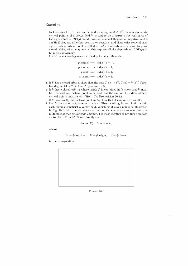
Exercises 113
Exercises
In Exercises 1–3, V is a vector field on a region Ω ⊂ R2. A nondegeneratecritical point p of a vector field V is said to be a source if the real parts ofthe eigenvalues of DV (p) are all positive, a sink if they are all negative, and asaddle if they are all either positive or negative, and there exist some of eachsign. Such a critical point is called a center if all orbits of V close to p areclosed orbits, which stay near p; this requires all the eigenvalues of DV (p) tobe purely imaginary.
1. Let V have a nondegenerate critical point at p. Show that
p saddle =⇒ indp(V ) = −1,
p source =⇒ indp(V ) = 1,
p sink =⇒ indp(V ) = 1,
p center =⇒ indp(V ) = 1.
2. If V has a closed orbit γ, show that the map T : γ → S1, T (x) = V (x)/|V (x)|,has degree +1. (Hint: Use Proposition 19.8.)
3. If V has a closed orbit γ whose inside O is contained in Ω, show that V musthave at least one critical point in O, and that the sum of the indices of suchcritical points must be +1. (Hint: Use Proposition 20.2.)If V has exactly one critical point in O, show that it cannot be a saddle.
4. Let M be a compact, oriented surface. Given a triangulation of M , withineach triangle construct a vector field, vanishing at seven points as illustratedin Fig. 20.1, with the vertices as attractors, the center as a repeller, and themidpoints of each side as saddle points. Fit these together to produce a smoothvector field X on M . Show directly that
Index(X) = V − E + F,
where
V = # vertices, E = # edges, F = # faces,
in the triangulation.
Figure 20.1
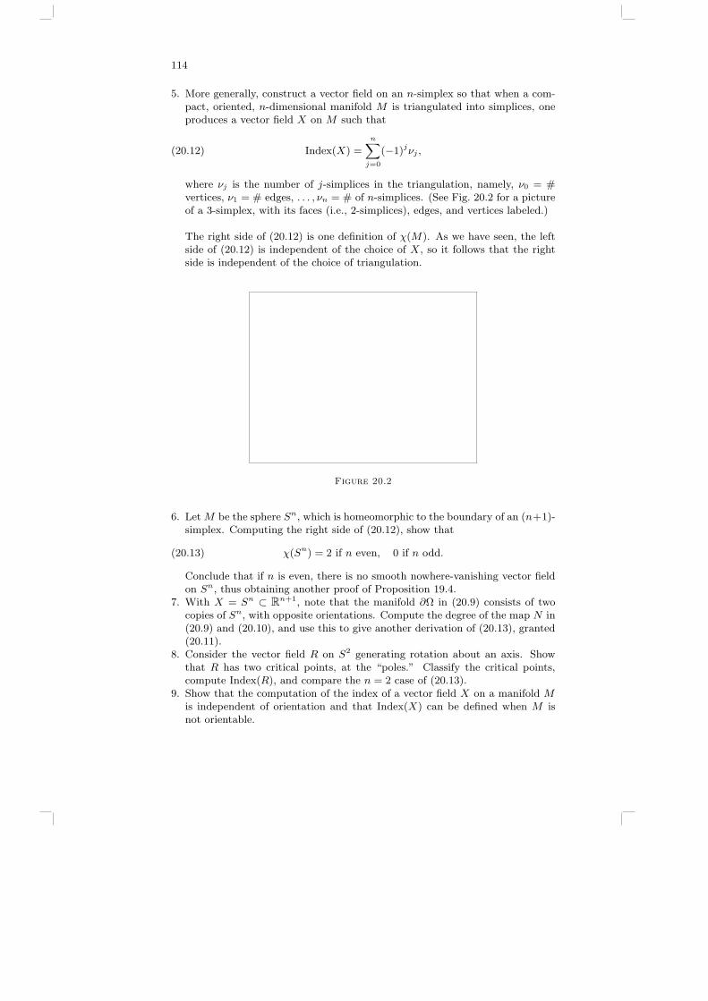
114
5. More generally, construct a vector field on an n-simplex so that when a com-pact, oriented, n-dimensional manifold M is triangulated into simplices, oneproduces a vector field X on M such that
(20.12) Index(X) =
n∑j=0
(−1)jνj ,
where νj is the number of j-simplices in the triangulation, namely, ν0 = #vertices, ν1 = # edges, . . . , νn = # of n-simplices. (See Fig. 20.2 for a pictureof a 3-simplex, with its faces (i.e., 2-simplices), edges, and vertices labeled.)
The right side of (20.12) is one definition of χ(M). As we have seen, the leftside of (20.12) is independent of the choice of X, so it follows that the rightside is independent of the choice of triangulation.
Figure 20.2
6. Let M be the sphere Sn, which is homeomorphic to the boundary of an (n+1)-simplex. Computing the right side of (20.12), show that
(20.13) χ(Sn) = 2 if n even, 0 if n odd.
Conclude that if n is even, there is no smooth nowhere-vanishing vector fieldon Sn, thus obtaining another proof of Proposition 19.4.
7. With X = Sn ⊂ Rn+1, note that the manifold ∂Ω in (20.9) consists of twocopies of Sn, with opposite orientations. Compute the degree of the map N in(20.9) and (20.10), and use this to give another derivation of (20.13), granted(20.11).
8. Consider the vector field R on S2 generating rotation about an axis. Showthat R has two critical points, at the “poles.” Classify the critical points,compute Index(R), and compare the n = 2 case of (20.13).
9. Show that the computation of the index of a vector field X on a manifold Mis independent of orientation and that Index(X) can be defined when M isnot orientable.
A. Nonsmooth vector fields 115
A. Nonsmooth vector fields
Here we establish properties of solutions to the ODE
(A.1)dy
dt= F (t, y), y(t0) = x0
of a sort done in §§2–6, under weaker hypotheses than those used there; inparticular, we do not require F to be Lipschitz in y. For existence, we canassume considerably less:
Proposition A.1. Let x0 ∈ O, an open subset of Rn, I ⊂ R an intervalcontaining t0. Assume F is continuous on I ×O. Then the equation (A.1)has a solution on some t-interval containing t0.
Proof. Without loss of generality, we can assume F is bounded and con-tinuous on R×Rn. Take Fj ∈ C∞(R×Rn) such that |Fj | ≤ K and Fj → Flocally uniformly, and let yj ∈ C∞(R) be the unique solution to
(A.2)dyj
dt= Fj(t, y), yj(t0) = x0,
whose existence is guaranteed by the material of §2. Thus
(A.3) yj(t) = x0 +∫ t
t0
Fj
(s, yj(s)
)ds.
Now
(A.4) |Fj | ≤ K =⇒ |yj(t′)− yj(t)| ≤ K|t′ − t|.Hence, by Ascoli’s theorem (see Proposition 6.2 in Appendix A, FunctionalAnalysis) the sequence (yj) has a subsequence (yjν ) which converges locallyuniformly: yjν → y. It follows immediately that
(A.5) y(t) = x0 +∫ t
t0
F(s, y(s)
)ds,
so y solves (A.1).
Under the hypotheses of Proposition A.1, a solution to (A.1) may notbe unique. The following family of examples illustrates the phenomenon.Take a ∈ (0, 1) and consider
(A.6)dy
dt= |y|a, y(0) = 0.
Then one solution on [0,∞) is given by
(A.7) y0(t) = (1− a)1/(1−a) t1/(1−a),
and another is given by
y∗(t) = 0.
116
Note that, for any ε > 0, the problem dy/dt = |y|a, y(0) = ε has a uniquesolution on t ∈ [0,∞), and limε→0 yε(t) = y0(t). Understanding thisprovides the key to the following uniqueness result, due to W. Osgood.
Let ω : R+ → R+ be a modulus of continuity, i.e., ω(0) = 0, ω iscontinuous, and increasing. We may as well assume ω is bounded and C∞
on (0,∞).
Proposition A.2. In the setting of Proposition A.1, assume F is contin-uous on I ×O and that
(A.8) |F (t, y1)− F (t, y2)| ≤ ω(|y1 − y2|
),
for all t ∈ I, yj ∈ O. Then solutions to (A.1) (with range in O) are unique,provided
(A.9)∫ 1
0
ds
ω(s)= ∞.
Proof. If y1(t) and y2(t) are two solutions to (A.1), then
(A.10) y1(t)− y2(t) =∫ t
t0
F
(s, y1(s)
)− F(s, y2(s)
)ds.
Let us set θ(t) = |y1(t)− y2(t)|. Hence, by (A.8), for t ≥ t0,
(A.11) θ(t) ≤∫ t
t0
ω(θ(s)
)ds.
In particular, for each ε > 0, θ(t) ≤ ∫ t
t0ω(θ(s) + ε
)ds. Since we are
assuming ω is smooth on (0,∞), we can apply the Gronwall inequality,derived in (5.19)–(5.21), to deduce that
(A.12) θ(t) ≤ ϕε(t), ∀ t ≥ t0, ε > 0,
where ϕε is uniquely defined on [t0,∞) by
(A.13) ϕ′ε(t) = ω(ϕε(t) + ε
), ϕε(t0) = 0.
Thus
(A.14)∫ ϕε(t)
0
dζ
ω(ζ + ε)= t− t0.
Now the hypothesis (A.9) implies
(A.15) limε0
ϕε(t) = 0, ∀ t ≥ t0,
so we have θ(t) = 0, for all t ≥ t0. Similarly, one shows θ(t) = 0, for t ≤ t0,and uniqueness is proved.

References 117
An important example to which Proposition A.2 applies is
(A.16) ω(s) = s log1s, s ≤ 1
2.
This arises in the study of ideal fluid flow, as will be seen in Chapter 17.A similar argument establishes continuous dependence on initial data. If
(A.17)dyj
dt= F (t, yj), yj(t0) = xj ,
then
(A.18) y1(t)− y2(t) = x1 − x2 +∫ t
t0
F
(s, y1(s)
)− F(s, y2(s)
)ds,
so θ12(t) = |y1(t)− y2(t)| satisfies
(A.19) θ12(t) ≤ |x1 − x2|+∫ t
t0
ω(θ12(s)
)ds.
An argument similar to that used above gives (for t ≥ t0)
(A.20) θ12(t) ≤ ϑ(|x1 − x2|, t),where, for a > 0, t ≥ t0, ϑ(a, t) is the unique solution to
(A.21) ∂tϑ = ω(ϑ), ϑ(a, t0) = a,
that is,
(A.22)∫ ϑ(a,t)
a
dζ
ω(ζ)= t− t0.
Again, the hypothesis (A.9) implies
(A.23) lima0
ϑ(a, t) = 0, ∀ t ≥ t0.
By (A.20), we have
(A.24) |y1(t)− y2(t)| ≤ ϑ(|x1 − x2|, t
),
for all t ≥ t0, and a similar argument works for t ≤ t0.
References
[AM] R. Abraham and J. Marsden, Foundations of Mechanics, Benjamin/Cummings,Reading, Mass., 1978.
[Ar] V. Arnold, Mathematical Methods of Classical Mechanics, Springer-Verlag,New York, 1978.
[Ar2] V. Arnold, Geometrical Methods in the Theory of Ordinary DifferentialEquations, Springer-Verlag, New York, 1983.
[Bir] G. D. Birkhoff, Dynamical Systems, AMS Colloq. Publ., Vol. 9, Provi-dence, R.I., 1927.
118
[Car] C. Caratheodory, Calculus of Variations and Partial Differential Equationsof the First Order, Holden-Day, San Francisco, 1965.
[Fed] H. Federer, Geometric Measure Theory, Springer-Verlag, New York, 1969.[Go] H. Goldstein, Classical Mechanics, Addison-Wesley, New York, 1950.[GS] V. Guillemin and S. Sternberg, Symplectic Techniques in Physics, Cam-
bridge Univ. Press, Cambridge, 1984.[Hal] J. Hale, Ordinary Differential Equations, Wiley, New York, 1969.[Har] P. Hartman, Ordinary Differential Equations, Baltimore, 1973.[HS] M. Hirsch and S. Smale, Differential Equations, Dynamical Systems, and
Linear Algebra, Academic Press, New York, 1974.[Ja] J. Jackson, Classical Electrodynamics, J. Wiley, New York, 1962.
[Kan] Y. Kannai, An elementary proof of the no-retraction theorem, Amer.Math. Monthly 88(1981), 264–268.
[Lef] S. Lefschetz, Differential Equations, Geometric Theory, J. Wiley, NewYork, 1957.
[LS] L. Loomis and S. Sternberg, Advanced Calculus, Addison-Wesley, NewYork, 1968.
[Mos] J. Moser, Stable and Random Motions in Dynamical Systems, PrincetonUniv. Press, Princeton, N.J., 1973.
[NS] V. Nemytskii and V. Stepanov, Qualitative Theory of Differential Equa-tions, Dover, New York, 1989.
[Poi] H. Poincare, Les Methodes Nouvelles de la Mecanique Celeste, Gauthier-Villars, 1899.
[Poo] W. Poor, Differential Geometric Structures, McGraw-Hill, New York, 1981.[Rin] W. Rindler, Essential Relativity, Springer, New York, 1977.[Spi] M. Spivak, A Comprehensive Introduction to Differential Geometry, Vols. 1–
5, Publish or Perish Press, Berkeley, 1979.[Stb] S. Sternberg, Lectures on Differential Geometry, Prentice Hall, New Jersey,
1964.[Sto] J. J. Stoker, Differential Geometry, Wiley-Interscience, New York, 1969.[Str] G. Strang, Linear Algebra and its Applications, Harcourt Brace Jovanovich,
San Diego, 1988.[TS] J. M. Thompson and H. Stewart, Nonlinear Dynamics and Chaos, J. Wiley,
New York, 1986.[Wh] E. Whittaker, A Treatise on the Analytical Dynamics of Particles and
Rigid Bodies, Dover, New York, 1944.[Wig] S. Wiggins, Introduction to Applied Dynamical Systems and Chaos, Springer-
Verlag, New York, 1990.