Basics in Geostatistics GeostatisticalMonte-Carlo methods ... · GeostatisticalMonte-Carlo methods: Conditional simulation ... Gaussian conditional simulation Classical approach 1

Basics in Geostatistics 3Geostatistical Monte-Carlo methods:

Conditional simulation

Hans Wackernagel

MINES ParisTech

NERSC • April 2013

http://hans.wackernagel.free.fr

http://hans.wackernagel.free.fr

Basic concepts

Geostatistics

Hans Wackernagel (MINES ParisTech) Basics in Geostatistics 3 NERSC • April 2013 2 / 34

Concepts

Geostatistical model

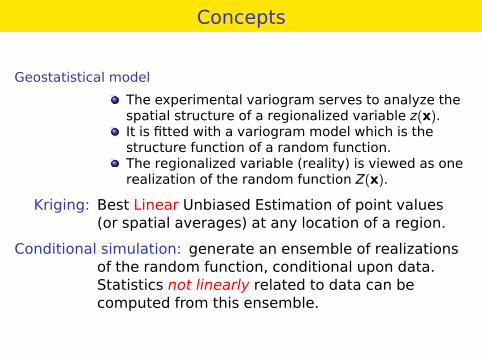
The experimental variogram serves to analyze thespatial structure of a regionalized variable z(x).It is fitted with a variogram model which is thestructure function of a random function.The regionalized variable (reality) is viewed as onerealization of the random function Z(x).

Kriging: Best Linear Unbiased Estimation of point values(or spatial averages) at any location of a region.

Conditional simulation: generate an ensemble of realizationsof the random function, conditional upon data.Statistics not linearly related to data can becomputed from this ensemble.

Concepts





Concepts





Limitations of linear geostatistics

Adequate for Gaussian random functions: in practice thedistribution function is often skew.

Probing with two-point statistics (covariance function,variogram): other tools are also available.

Need for non-linear estimates,e.g. for estimating probability of exceeding:

environmental threshold,cut-off grade in mining.

Conditional simulation techniques address all these aspects.

Gaussian conditional simulation generates an ensemble ofrealizations on which non-linear statistics can be readilycomputed.

Random functions: spatial correlation structure

Stationary random function:

mean, variance and spatial distribution function exist,

spatial correlation is described by the covariance function:

C(h) = E[(Z(x+h)−m) · (Z(x)−m)]

the variogram of a stationary random function is given bythe formula:

γ(h) = C(0)− C(h)

Gaussian conditional simulationClassical approach

1 Simulate realizations of a stationary Gaussian randomfunction with known covariance function C(h).

2 Condition the realizations using simple kriging.

Gaussian simulation

1) Unconditional simulation of a Gaussian RF


Simulation of a Gaussian random functionTurning bands method (TBM)

The simulation of realizations of a GRF can be done simply:determine the 1D covariance function of a corresponding 2D or 3Dcovariance model,generate directions θ1, . . . , θKsimulate realizations of 1D processes Y1, . . . ,YK along lines in thosedirections,project a given point on the lines and combine the correspondingsimulated values to obtain the simulated value of the 3D process atthat point:

Y(x) =1√K

K∑k=1

Yk(< x, θk >) for x ∈ D.

1D covariance function corresponding to2D or 3D isotropic covariance

The following formulas rely on Bochner’s theorem,in 3D:

C3D(h) =∫ 1

0C1D(t h)dt and C1D(h) =

ddh

(hC3D(h))

in 2D:

C2D(h) =1π

∫ π

0C1D(h sin θ)dθ and C1D(h) = 1+ h

∫ π/2

0

dC2D

dh(h sin θ)dθ

Example: exponential covariance function

The 1D model associated to a 3D exponential covariance is:

C1D(h) =(

1− ha

)exp

(−ha

)with h,a ≥ 0

Migration method: compute Poisson points, split intervalsinto halves set to ±1 (mean interval length is 2a):

TBM: exponential covariance

Gaussian simulation

2) Conditional simulation of a Gaussian RF


Best linear unbiased estimation (BLUE): kriging

Estimation of a value Z? at a location x0 in geographical spaceis performed using a linear combination of weights wα withdata at neighboring locations xα, α = 1, . . . ,n.

Kriging with known mean m (simple kriging):

Z?(x0) = m+n∑

α=1

wα (Z(xα)−m)

Conditional simulation of Gaussian RF

ZCS(x) = Z?(x)︸︷︷︸kriged from data

+ (ZS(x)− Z?S(x))︸︷︷︸simulated kriging error

( − )

+

=

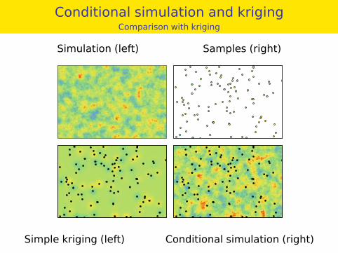
Conditional simulation and krigingComparison with kriging

Simulation (left) Samples (right)

Simple kriging (left) Conditional simulation (right)

Conditional simulation and kriging

Conditionally on the data,

the mean of conditional simulations is equal to the kriging:

E[ZCS(x) |Z(xα), α= 1, . . . ,n

]= Z?(x),

the variance of the conditional simulations is the krigingvariance:

var(ZCS(x) |Z(xα), α= 1, . . . ,n) = var(ZS(x)− Z?S(x)) = σ2K(x).

Gaussian simulationwith non-Gaussian data

1 Fit of a Gaussian anamorphosis function Z(x) = ϕ(Y(x)).2 Transform the data to

Gaussian values: Y(xα) = ϕ−1(Z(xα)).3 Fit the variogram of

the Gaussian random function Y(x).4 Simulate realizations YS(x).5 Condition YS(x) with Y(xα), thus obtaining YCS(x).6 Transform the result to

the initial scale: ZCS(x) = ϕ(YCS(x)).7 Compute various statistics on

the ensemble of realizations.

Case study

Simulating Yeu islandThe island is located off the south-west coast of Bretagne

Measurements of elevation in the sea (depths).


Kriging the elevation data

Negative kriging estimates are set to zero (below sea level).

Conditional simulation of elevation9 realizations of Yeu island

Simulation profiles along island

Probability that elevation is above sea level

Estimation of surface (km²) of Yeu island

2

Real From kriging Sim. min Sim. mean Sim. maxSurface 23.3 22.9 15.4 23.2 31.9

From conditional simulation the volume is estimated to be: 0.188 km3

(as compared to the value deduced from kriging results: 0.169 km3)

Conclusion

Summary

Gaussian random function simulations

Adequate for simulating Gaussian random functions

Anamorphosis to apply them to non-Gaussian data

Satisfy the need for non-linear estimates,e.g. for estimating probability of exceeding:

environmental thresholdcut-off grade in mining

Generate an ensemble of realisations on which non-linearstatistics are readily computed.

However, in a number of applications there is a need forstochastic models beyond the random functions framework...


Conclusion

Summary

Gaussian random function simulations

Adequate for simulating Gaussian random functions

Anamorphosis to apply them to non-Gaussian data

Satisfy the need for non-linear estimates,e.g. for estimating probability of exceeding:

environmental thresholdcut-off grade in mining

Generate an ensemble of realisations on which non-linearstatistics are readily computed.

However, in a number of applications there is a need forstochastic models beyond the random functions framework...


References

M Armstrong, A G Galli, H Beucher, G Le Loc’h, D Renard,B Doligez, R Eschard, and F Geffroy.Plurigaussian Simulations in Geosciences.Springer-Verlag, Berlin, 2nd edition, 2011.

JP Chilès and P Delfiner.Geostatistics: Modeling Spatial Uncertainty.Wiley, New York, 2nd edition, 2012.

C Lantuéjoul.Geostatistical Simulation: Models and Algorithms.Springer-Verlag, Berlin, 2002.

G. Matheron.Random Sets and Integral Geometry.John Wiley & Sons, New York, 1975.

RGeoS case-study

Conditional simulation example with RGeoS9.1.2

Code from the document Doc2D.pdf on the site:http://rgeos.free.fr


http://rgeos.free.fr

Loading the soil pollution data setlibrary(RGeoS)data(Exdemo_2D_pollution.table)DAT=Exdemo_2D_pollution.table

data.db = db.create(DAT,flag.grid=FALSE,ndim=2,autoname=F)

data.db = db.locate(data.db,"Zn","z",1)plot(data.db,pch=21,bg.in="black",title="Zn Sample locations")# suppress two outliershist(DAT$Zn,n=20)data.db = db.sel(data.db,Zn<20)hist(DAT$Zn[DAT$Zn<20])

110 115 120 125 130 135 140

485

490

495

500

505

510

●

●

●

●

●

●

●

●

●

●

●●

●

●

●

●

● ●

●

●

●

● ●

●

●

●

● ●●

●

●

●

●

●

●

●

●

●

●

●

●●

●

●

●

●●●

●

●●

●

●

●

●●

●

●●

●

●

●

●

●

●

●

●

● ●

●

●

●

● ●

●

●

●

●

●

●

●

●

●

●

●●

●

●

●

●●

●

●

●

●

●

●

●

●

●

●

Zn Sample locations Histogram of DAT$Zn

DAT$Zn

Fre

quen

cy

5 10 15 20 25 30

010

2030

4050

Structural analysisdata.vario = vario.calc(data.db,lag=1,nlag=10)plot(data.vario,npairdw=TRUE,npairpt=TRUE)

data.4dir.vario =vario.calc(data.db,lag=1,nlag=10,dir=c(0,45,90,135))

plot(data.4dir.vario,title="Directional variograms")

data.model = model.auto(data.vario,

struct=c("Spherical","Exponential"),title="Modelling omni-directional variogram")

2 4 6 8

0.5

1.0

1.5

2.0

2.5

3.0

●

●

●

●

●

●●

●●

●

3

123

183

205

231

229198

187204

184

2 4 6 80.

51.

01.

52.

02.

53.

0

Modelling omni−directional variogram

2 4 6 80.

51.

01.

52.

02.

53.

0

Kriging

# for KRIGING use all 102 data (suppress selection)data.db = db.sel(data.db)#kriging gridgrid.db = db.grid.init(data.db,nodes=c(100,90))# defining unique neighborhooddata.unique = neigh.input(ndim=2)data.db = db.locate(data.db,seq(8,9))data.db = db.locate(data.db,Zn,z)grid.db = kriging(data.db,grid.db,data.model,data.unique,radix="KU")

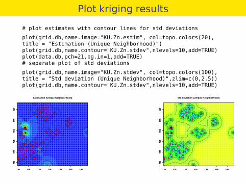
Plot kriging results

# plot estimates with contour lines for std deviations

plot(grid.db,name.image="KU.Zn.estim", col=topo.colors(20),title = "Estimation (Unique Neighborhood)")plot(grid.db,name.contour="KU.Zn.stdev",nlevels=10,add=TRUE)plot(data.db,pch=21,bg.in=1,add=TRUE)# separate plot of std deviations

plot(grid.db,name.image="KU.Zn.stdev", col=topo.colors(100),title = "Std deviation (Unique Neighborhood)",zlim=c(0,2.5))plot(grid.db,name.contour="KU.Zn.stdev",nlevels=10,add=TRUE)

110 115 120 125 130 135 140

485

490

495

500

505

510

Estimation (Unique Neighborhood)

110 115 120 125 130 135 140

485

490

495

500

505

510

0.8

0.8

0.8

0.8

0.8

1

1

1

1

1

1

1

1

1

1

1

1

1

1

1

1

1

1

1

1

1

1

1

1 1

1

1

1

1

1

1

1

1

1

1

1

1

1

1

1

1

1.2

1.2

1.2

1.2 1.2

1.2

1.2

1.2

1.4

1.4

1.4

1.4

1.4

1.4

1.6

1.6

1.6

1.6

1.6

110 115 120 125 130 135 140

485

490

495

500

505

510

●

●

●

●

●

●

●

●

●

●

●●

●

●

●

●

● ●

●

●

●

● ●

●

●

●

● ●●

●

●

●

●

●

●

●

●

●

●

●

●●

●

●

●

●●

●

●

●●

●

●

●

●●

●

●●

●

●

●

●

●

●

●

●

● ●

●

●

●

● ●

●

●

●

●

●

●

●

●

●

●

●●

●

●

●

●

●

●

●

●

●

●

●

●

●

●

●

110 115 120 125 130 135 140

485

490

495

500

505

510

Std deviation (Unique Neighborhood)

110 115 120 125 130 135 140

485

490

495

500

505

510

0.8

0.8

0.8

0.8

0.8

1

1

1

1

1

1

1

1

1

1

1

1

1

1

1

1

1

1

1

1

1

1

1

1 1

1

1

1

1

1

1

1

1

1

1

1

1

1

1

1

1

1.2

1.2

1.2

1.2 1.2

1.2

1.2

1.2

1.4

1.4

1.4

1.4

1.4

1.4

1.6

1.6

1.6

1.6

1.6

110 115 120 125 130 135 140

485

490

495

500

505

510

●

●

●

●

●

●

●

●

●

●

●●

●

●

●

●

● ●

●

●

●

● ●

●

●

●

● ●●

●

●

●

●

●

●

●

●

●

●

●

●●

●

●

●

●●

●

●

●●

●

●

●

●●

●

●●

●

●

●

●

●

●

●

●

● ●

●

●

●

● ●

●

●

●

●

●

●

●

●

●

●

●●

●

●

●

●

●

●

●

●

●

●

●

●

●

●

●

Anamorphosis

## anamorphosis (normal score transform & Hermite poly)data.anam=anam.fit(data.db,"Zn")# transform z to Gaussian ydata.db = anam.z2y(data.db,"Zn",anam=data.anam)data.g.vario = vario.calc(data.db,nlag=10,lag=1)plot(data.g.vario,npairdw=TRUE,npairpt=TRUE)data.g.model = model.auto(data.g.vario,struct=c("Exponential"))

−2 −1 0 1 2

510

1520

2530

Gaussian

Raw

−2 −1 0 1 2

510

1520

2530

2 4 6 80.

20.

40.

60.

81.

01.

2

●

●

●

●

●

● ●●

●

●

3

127

187

209

234

233 202194

218

198

Conditional simulation10 realizations (100 turning bands)

grid.db = simtub(data.db,grid.db,data.g.model,data.unique,nbsimu=10,nbtuba=100)# transform back from Gaussian Y to Zgrid.db = anam.y2z(grid.db,ngrep="Simu.Gaussian.Zn",anam=data.anam)

plot(grid.db,name.image="Raw.Simu.Gaussian.Zn.S1",col=topo.colors(20))plot(data.db,pch=21,bg.in=1,add=TRUE)

plot(grid.db,name.image="Raw.Simu.Gaussian.Zn.S10",col=topo.colors(20))plot(data.db,pch=21,bg.in=1,add=TRUE)

110 115 120 125 130 135 140

485

490

495

500

505

510

Raw.Simu.Gaussian.Zn.S1

110 115 120 125 130 135 140

485

490

495

500

505

510

●

●

●

●

●

●

●

●

●

●●●

●

●

●

●

● ●●

●

●

●●

●

●

●

● ●●

●

●

●●

●●

●

●

●

●

●

●●

●

●

●

●●●●

● ●

●

●

●

●●

●●●

●

●

●●

●

●

●

●●●

●

●

●

●●

●●

●

●

●

●

●

●

●

●

●●

●●

●

●●

●

●

●

●

●

●

●

●

●

●

110 115 120 125 130 135 140

485

490

495

500

505

510

Raw.Simu.Gaussian.Zn.S2

110 115 120 125 130 135 140

485

490

495

500

505

510

●

●

●

●

●

●

●

●

●

●●●

●

●

●

●

● ●●

●

●

●●

●

●

●

● ●●

●

●

●●

●●

●

●

●

●

●

●●

●

●

●

●●●●

● ●

●

●

●

●●

●●●

●

●

●●

●

●

●

●●●

●

●

●

●●

●●

●

●

●

●

●

●

●

●

●●

●●

●

●●

●

●

●

●

●

●

●

●

●

●

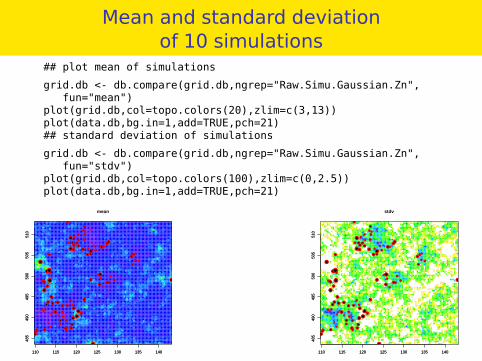
Mean and standard deviationof 10 simulations

## plot mean of simulations

grid.db <- db.compare(grid.db,ngrep="Raw.Simu.Gaussian.Zn",fun="mean")

plot(grid.db,col=topo.colors(20),zlim=c(3,13))plot(data.db,bg.in=1,add=TRUE,pch=21)## standard deviation of simulations

grid.db <- db.compare(grid.db,ngrep="Raw.Simu.Gaussian.Zn",fun="stdv")

plot(grid.db,col=topo.colors(100),zlim=c(0,2.5))plot(data.db,bg.in=1,add=TRUE,pch=21)

110 115 120 125 130 135 140

485

490

495

500

505

510

mean

110 115 120 125 130 135 140

485

490

495

500

505

510

●

●

●

●

●

●

●

●

●

●●●

●

●

●

●

● ●●

●

●

●●

●

●

●

● ●●

●

●

●●

●●

●

●

●

●

●

●●

●

●

●

●●●●

● ●

●

●

●

●●

●●●

●

●

●●

●

●

●

●●●

●

●

●

●●

●●

●

●

●

●

●

●

●

●

●●

●●

●

●●

●

●

●

●

●

●

●

●

●

●

110 115 120 125 130 135 140

485

490

495

500

505

510

stdv

110 115 120 125 130 135 140

485

490

495

500

505

510

●

●

●

●

●

●

●

●

●

●●●

●

●

●

●

● ●●

●

●

●●

●

●

●

● ●●

●

●

●●

●●

●

●

●

●

●

●●

●

●

●

●●●●

● ●

●

●

●

●●

●●●

●

●

●●

●

●

●

●●●

●

●

●

●●

●●

●

●

●

●

●

●

●

●

●●

●●

●

●●

●

●

●

●

●

●

●

●

●

●

Exporting the resultsPlotting them with the lattice package

grid.db # to find out the names of columnsSmean=db.extract(grid.db,"mean"); Sstdv=db.extract(grid.db,"stdv")x1=db.extract(grid.db,"x1"); x2=db.extract(grid.db,"x2")library(lattice) # a standard graphical package in R

levelplot(Smean~x1*x2,main="Mean of 10 simulations",col.regions=topo.colors)

levelplot(Sstdv~x1*x2,

main="Std deviation of 10 simulations",col.regions=rainbow(20, start=.5, end=0.01))

Mean of 10 simulations

x1

x2

485

490

495

500

505

510

115 120 125 130 135 140

5

10

15

20

25

Std deviation of 10 simulations

x1

x2

485

490

495

500

505

510

115 120 125 130 135 140

0

2

4

6

8

10

12

Documents

Basics in Geostatistics GeostatisticalMonte-Carlo methods ... · GeostatisticalMonte-Carlo methods: Conditional simulation ... Gaussian conditional simulation Classical approach 1