Embed Size (px)
Citation preview
This is page 162Printer: Opaque this
6Basics of Euclidean Geometry
Rien n’est beau que le vrai.
—Hermann Minkowski
6.1 Inner Products, Euclidean Spaces
In affine geometry it is possible to deal with ratios of vectors and barycen-ters of points, but there is no way to express the notion of length of a linesegment or to talk about orthogonality of vectors. A Euclidean structureallows us to deal with metric notions such as orthogonality and length (ordistance).
This chapter and the next two cover the bare bones of Euclidean ge-ometry. One of our main goals is to give the basic properties of thetransformations that preserve the Euclidean structure, rotations and re-flections, since they play an important role in practice. As affine geometryis the study of properties invariant under bijective affine maps and projec-tive geometry is the study of properties invariant under bijective projectivemaps, Euclidean geometry is the study of properties invariant under certainaffine maps called rigid motions. Rigid motions are the maps that preservethe distance between points. Such maps are, in fact, affine and bijective (atleast in the finite–dimensional case; see Lemma 7.4.3). They form a groupIs(n) of affine maps whose corresponding linear maps form the group O(n)of orthogonal transformations. The subgroup SE(n) of Is(n) correspondsto the orientation–preserving rigid motions, and there is a corresponding
6.1. Inner Products, Euclidean Spaces 163
subgroup SO(n) of O(n), the group of rotations. These groups play a veryimportant role in geometry, and we will study their structure in some detail.
Before going any further, a potential confusion should be cleared up.
Euclidean geometry deals with affine spaces(E,
−→E)
where the associated
vector space−→E is equipped with an inner product. Such spaces are called
Euclidean affine spaces. However, inner products are defined on vectorspaces. Thus, we must first study the properties of vector spaces equippedwith an inner product, and the linear maps preserving an inner product(the orthogonal group SO(n)). Such spaces are called Euclidean spaces(omitting the word affine). It should be clear from the context whether weare dealing with a Euclidean vector space or a Euclidean affine space, butwe will try to be clear about that. For instance, in this chapter, exceptfor Definition 6.2.9, we are dealing with Euclidean vector spaces and linearmaps.
We begin by defining inner products and Euclidean spaces. The Cauchy–Schwarz inequality and the Minkowski inequality are shown. We defineorthogonality of vectors and of subspaces, orthogonal bases, and orthonor-mal bases. We offer a glimpse of Fourier series in terms of the orthogonalfamilies (sin px)p≥1∪(cos qx)q≥0 and (eikx)k∈Z. We prove that every finite–dimensional Euclidean space has orthonormal bases. Orthonormal basesare the Euclidean analogue for affine frames. The first proof uses dual-ity, and the second one the Gram–Schmidt orthogonalization procedure.The QR-decomposition for invertible matrices is shown as an applicationof the Gram–Schmidt procedure. Linear isometries (also called orthogonaltransformations) are defined and studied briefly. We conclude with a shortsection in which some applications of Euclidean geometry are sketched.One of the most important applications, the method of least squares, isdiscussed in Chapter 13.
For a more detailed treatment of Euclidean geometry, see Berger [12, 13],Snapper and Troyer [160], or any other book on geometry, such as Pedoe[136], Coxeter [35], Fresnel [66], Tisseron [169], or Cagnac, Ramis, andCommeau [25]. Serious readers should consult Emil Artin’s famous book[4], which contains an in-depth study of the orthogonal group, as well asother groups arising in geometry. It is still worth consulting some of theolder classics, such as Hadamard [81, 82] and Rouche and de Comberousse[144]. The first edition of [81] was published in 1898, and finally reachedits thirteenth edition in 1947! In this chapter it is assumed that all vectorspaces are defined over the field R of real numbers unless specified otherwise(in a few cases, over the complex numbers C).
First, we define a Euclidean structure on a vector space. Technically,a Euclidean structure over a vector space E is provided by a symmetricbilinear form on the vector space satisfying some extra properties. Recallthat a bilinear form ϕ:E × E → R is definite if for every u ∈ E, u 6= 0implies that ϕ(u, u) 6= 0, and positive if for every u ∈ E, ϕ(u, u) ≥ 0.
164 6. Basics of Euclidean Geometry
Definition 6.1.1 A Euclidean space is a real vector space E equippedwith a symmetric bilinear form ϕ:E × E → R that is positive definite.More explicitly, ϕ:E × E → R satisfies the following axioms:
ϕ(u1 + u2, v) = ϕ(u1, v) + ϕ(u2, v),
ϕ(u, v1 + v2) = ϕ(u, v1) + ϕ(u, v2),
ϕ(λu, v) = λϕ(u, v),
ϕ(u, λv) = λϕ(u, v),
ϕ(u, v) = ϕ(v, u),
u 6= 0 implies that ϕ(u, u) > 0.
The real number ϕ(u, v) is also called the inner product (or scalar product)of u and v. We also define the quadratic form associated with ϕ as thefunction Φ:E → R+ such that
Φ(u) = ϕ(u, u),
for all u ∈ E.
Since ϕ is bilinear, we have ϕ(0, 0) = 0, and since it is positive definite,we have the stronger fact that
ϕ(u, u) = 0 iff u = 0,
that is, Φ(u) = 0 iff u = 0.Given an inner product ϕ:E × E → R on a vector space E, we also
denote ϕ(u, v) by
u · v or 〈u, v〉 or (u|v),
and√
Φ(u) by ‖u‖.
Example 6.1 The standard example of a Euclidean space is Rn, under
the inner product · defined such that
(x1, . . . , xn) · (y1, . . . , yn) = x1y1 + x2y2 + · · · + xnyn.
There are other examples.
Example 6.2 For instance, let E be a vector space of dimension 2, andlet (e1, e2) be a basis of E. If a > 0 and b2 − ac < 0, the bilinear formdefined such that
ϕ(x1e1 + y1e2, x2e1 + y2e2) = ax1x2 + b(x1y2 + x2y1) + cy1y2
yields a Euclidean structure on E. In this case,
Φ(xe1 + ye2) = ax2 + 2bxy + cy2.
Example 6.3 Let C[a, b] denote the set of continuous functions f : [a, b] →R. It is easily checked that C[a, b] is a vector space of infinite dimension.
6.1. Inner Products, Euclidean Spaces 165
Given any two functions f, g ∈ C[a, b], let
〈f, g〉 =
∫ b
a
f(t)g(t)dt.
We leave as an easy exercise that 〈−,−〉 is indeed an inner product onC[a, b]. In the case where a = −π and b = π (or a = 0 and b = 2π, thismakes basically no difference), one should compute
〈sin px, sin qx〉, 〈sin px, cos qx〉, and 〈cos px, cos qx〉,for all natural numbers p, q ≥ 1. The outcome of these calculations is whatmakes Fourier analysis possible!
Let us observe that ϕ can be recovered from Φ. Indeed, by bilinearityand symmetry, we have
Φ(u+ v) = ϕ(u+ v, u+ v)
= ϕ(u, u+ v) + ϕ(v, u+ v)
= ϕ(u, u) + 2ϕ(u, v) + ϕ(v, v)
= Φ(u) + 2ϕ(u, v) + Φ(v).
Thus, we have
ϕ(u, v) =1
2[Φ(u+ v) − Φ(u) − Φ(v)].
We also say that ϕ is the polar form of Φ. We will generalize polar formsto polynomials, and we will see that they play a very important role.
One of the very important properties of an inner product ϕ is that themap u 7→
√Φ(u) is a norm.
Lemma 6.1.2 Let E be a Euclidean space with inner product ϕ, and let Φbe the corresponding quadratic form. For all u, v ∈ E, we have the Cauchy–Schwarz inequality
ϕ(u, v)2 ≤ Φ(u)Φ(v),
the equality holding iff u and v are linearly dependent.We also have the Minkowski inequality
√Φ(u+ v) ≤
√Φ(u) +
√Φ(v),
the equality holding iff u and v are linearly dependent, where in addition ifu 6= 0 and v 6= 0, then u = λv for some λ > 0.
Proof . For any vectors u, v ∈ E, we define the function T : R → R suchthat
T (λ) = Φ(u+ λv),
for all λ ∈ R. Using bilinearity and symmetry, we have
Φ(u+ λv) = ϕ(u+ λv, u+ λv)
166 6. Basics of Euclidean Geometry
= ϕ(u, u+ λv) + λϕ(v, u+ λv)
= ϕ(u, u) + 2λϕ(u, v) + λ2ϕ(v, v)
= Φ(u) + 2λϕ(u, v) + λ2Φ(v).
Since ϕ is positive definite, Φ is nonnegative, and thus T (λ) ≥ 0 for allλ ∈ R. If Φ(v) = 0, then v = 0, and we also have ϕ(u, v) = 0. In this case,the Cauchy–Schwarz inequality is trivial, and v = 0 and u are linearlydependent.
Now, assume Φ(v) > 0. Since T (λ) ≥ 0, the quadratic equation
λ2Φ(v) + 2λϕ(u, v) + Φ(u) = 0
cannot have distinct real roots, which means that its discriminant
∆ = 4(ϕ(u, v)2 − Φ(u)Φ(v))
is null or negative, which is precisely the Cauchy–Schwarz inequality
ϕ(u, v)2 ≤ Φ(u)Φ(v).
If
ϕ(u, v)2 = Φ(u)Φ(v),
then the above quadratic equation has a double root λ0, and we haveΦ(u+ λ0v) = 0. If λ0 = 0, then ϕ(u, v) = 0, and since Φ(v) > 0, we musthave Φ(u) = 0, and thus u = 0. In this case, of course, u = 0 and v arelinearly dependent. Finally, if λ0 6= 0, since Φ(u + λ0v) = 0 implies thatu+ λ0v = 0, then u and v are linearly dependent. Conversely, it is easy tocheck that we have equality when u and v are linearly dependent.
The Minkowski inequality√
Φ(u+ v) ≤√
Φ(u) +√
Φ(v)
is equivalent to
Φ(u+ v) ≤ Φ(u) + Φ(v) + 2√
Φ(u)Φ(v).
However, we have shown that
2ϕ(u, v) = Φ(u+ v) − Φ(u) − Φ(v),
and so the above inequality is equivalent to
ϕ(u, v) ≤√
Φ(u)Φ(v),
which is trivial when ϕ(u, v) ≤ 0, and follows from the Cauchy–Schwarzinequality when ϕ(u, v) ≥ 0. Thus, the Minkowski inequality holds. Finally,assume that u 6= 0 and v 6= 0, and that
√Φ(u+ v) =
√Φ(u) +
√Φ(v).
When this is the case, we have
ϕ(u, v) =√
Φ(u)Φ(v),
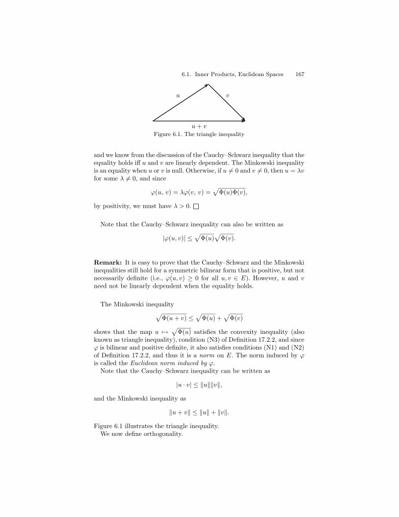
6.1. Inner Products, Euclidean Spaces 167
u v
u+ vFigure 6.1. The triangle inequality
and we know from the discussion of the Cauchy–Schwarz inequality that theequality holds iff u and v are linearly dependent. The Minkowski inequalityis an equality when u or v is null. Otherwise, if u 6= 0 and v 6= 0, then u = λvfor some λ 6= 0, and since
ϕ(u, v) = λϕ(v, v) =√
Φ(u)Φ(v),
by positivity, we must have λ > 0.
Note that the Cauchy–Schwarz inequality can also be written as
|ϕ(u, v)| ≤√
Φ(u)√
Φ(v).
Remark: It is easy to prove that the Cauchy–Schwarz and the Minkowskiinequalities still hold for a symmetric bilinear form that is positive, but notnecessarily definite (i.e., ϕ(u, v) ≥ 0 for all u, v ∈ E). However, u and vneed not be linearly dependent when the equality holds.
The Minkowski inequality√
Φ(u+ v) ≤√
Φ(u) +√
Φ(v)
shows that the map u 7→√
Φ(u) satisfies the convexity inequality (alsoknown as triangle inequality), condition (N3) of Definition 17.2.2, and sinceϕ is bilinear and positive definite, it also satisfies conditions (N1) and (N2)of Definition 17.2.2, and thus it is a norm on E. The norm induced by ϕis called the Euclidean norm induced by ϕ.
Note that the Cauchy–Schwarz inequality can be written as
|u · v| ≤ ‖u‖‖v‖,
and the Minkowski inequality as
‖u+ v‖ ≤ ‖u‖ + ‖v‖.
Figure 6.1 illustrates the triangle inequality.We now define orthogonality.
168 6. Basics of Euclidean Geometry
6.2 Orthogonality, Duality, Adjoint of a LinearMap
An inner product on a vector space gives the ability to define the notionof orthogonality. Families of nonnull pairwise orthogonal vectors must belinearly independent. They are called orthogonal families. In a vector spaceof finite dimension it is always possible to find orthogonal bases. This isvery useful theoretically and practically. Indeed, in an orthogonal basis,finding the coordinates of a vector is very cheap: It takes an inner product.Fourier series make crucial use of this fact. When E has finite dimension, weprove that the inner product on E induces a natural isomorphism betweenE and its dual space E∗. This allows us to define the adjoint of a linearmap in an intrinsic fashion (i.e., independently of bases). It is also possibleto orthonormalize any basis (certainly when the dimension is finite). Wegive two proofs, one using duality, the other more constructive using theGram–Schmidt orthonormalization procedure.
Definition 6.2.1 Given a Euclidean space E, any two vectors u, v ∈ E areorthogonal, or perpendicular , if u · v = 0. Given a family (ui)i∈I of vectorsin E, we say that (ui)i∈I is orthogonal if ui · uj = 0 for all i, j ∈ I, wherei 6= j. We say that the family (ui)i∈I is orthonormal if ui · uj = 0 for alli, j ∈ I, where i 6= j, and ‖ui‖ = ui · ui = 1, for all i ∈ I. For any subset Fof E, the set
F⊥ = v ∈ E | u · v = 0, for all u ∈ F,of all vectors orthogonal to all vectors in F , is called the orthogonalcomplement of F .
Since inner products are positive definite, observe that for any vectoru ∈ E, we have
u · v = 0 for all v ∈ E iff u = 0.
It is immediately verified that the orthogonal complement F⊥ of F is asubspace of E.
Example 6.4 Going back to Example 6.3 and to the inner product
〈f, g〉 =
∫ π
−π
f(t)g(t)dt
on the vector space C[−π, π], it is easily checked that
〈sin px, sin qx〉 =
π if p = q, p, q ≥ 1,0 if p 6= q, p, q ≥ 1,
〈cos px, cos qx〉 =
π if p = q, p, q ≥ 1,0 if p 6= q, p, q ≥ 0,
6.2. Orthogonality, Duality, Adjoint of a Linear Map 169
and
〈sin px, cos qx〉 = 0,
for all p ≥ 1 and q ≥ 0, and of course, 〈1, 1〉 =∫ π
−πdx = 2π.
As a consequence, the family (sin px)p≥1∪ (cos qx)q≥0 is orthogonal. It isnot orthonormal, but becomes so if we divide every trigonometric functionby
√π, and 1 by
√2π.
Remark: Observe that if we allow complex–valued functions, we obtainsimpler proofs. For example, it is immediately checked that
∫ π
−π
eikxdx =
2π if k = 0,0 if k 6= 0,
because the derivative of eikx is ikeikx.
Ä However, beware that something strange is going on. Indeed,unless k = 0, we have
〈eikx, eikx〉 = 0,
since
〈eikx, eikx〉 =
∫ π
−π
(eikx)2dx =
∫ π
−π
ei2kxdx = 0.
The inner product 〈eikx, eikx〉 should be strictly positive. What wentwrong?
The problem is that we are using the wrong inner product. When we usecomplex-valued functions, we must use the Hermitian inner product
〈f, g〉 =
∫ π
−π
f(x)g(x)dx,
where g(x) is the conjugate of g(x). The Hermitian inner product is notsymmetric. Instead,
〈g, f〉 = 〈f, g〉.(Recall that if z = a + ib, where a, b ∈ R, then z = a − ib. Also, eiθ =cos θ + i sin θ). With the Hermitian inner product, everything works outbeautifully! In particular, the family (eikx)k∈Z is orthogonal. Hermitianspaces and some basics of Fourier series will be discussed more rigorouslyin Chapter 10.
We leave the following simple two results as exercises.
Lemma 6.2.2 Given a Euclidean space E, for any family (ui)i∈I ofnonnull vectors in E, if (ui)i∈I is orthogonal, then it is linearly independent.
170 6. Basics of Euclidean Geometry
Lemma 6.2.3 Given a Euclidean space E, any two vectors u, v ∈ E areorthogonal iff
‖u+ v‖2 = ‖u‖2 + ‖v‖2.
One of the most useful features of orthonormal bases is that they afforda very simple method for computing the coordinates of a vector over anybasis vector. Indeed, assume that (e1, . . . , em) is an orthonormal basis. Forany vector
x = x1e1 + · · · + xmem,
if we compute the inner product x · ei, we get
x · ei = x1e1 · ei + · · · + xiei · ei + · · · + xmem · ei = xi,
since
ei · ej =
1 if i = j,0 if i 6= j
is the property characterizing an orthonormal family. Thus,
xi = x · ei,
which means that xiei = (x · ei)ei is the orthogonal projection of x ontothe subspace generated by the basis vector ei. If the basis is orthogonal butnot necessarily orthonormal, then
xi =x · ei
ei · ei
=x · ei
‖ei‖2.
All this is true even for an infinite orthonormal (or orthogonal) basis (ei)i∈I .
Ä However, remember that every vector x is expressed as a linearcombination
x =∑
i∈I
xiei
where the family of scalars (xi)i∈I has finite support, which means thatxi = 0 for all i ∈ I − J , where J is a finite set. Thus, even though thefamily (sin px)p≥1 ∪ (cos qx)q≥0 is orthogonal (it is not orthonormal, butbecomes so if we divide every trigonometric function by
√π, and 1 by
√2π;
we won’t because it looks messy!), the fact that a function f ∈ C0[−π, π]can be written as a Fourier series as
f(x) = a0 +∞∑
k=1
(ak cos kx+ bk sin kx)
does not mean that (sin px)p≥1 ∪ (cos qx)q≥0 is a basis of this vector spaceof functions, because in general, the families (ak) and (bk) do not have
6.2. Orthogonality, Duality, Adjoint of a Linear Map 171
finite support! In order for this infinite linear combination to make sense,it is necessary to prove that the partial sums
a0 +
n∑
k=1
(ak cos kx+ bk sin kx)
of the series converge to a limit when n goes to infinity. This requires atopology on the space.
Still, a small miracle happens. If f ∈ C[−π, π] can indeed be expressedas a Fourier series
f(x) = a0 +∞∑
k=1
(ak cos kx+ bk sin kx),
the coefficients a0 and ak, bk, k ≥ 1, can be computed by projecting f overthe basis functions, i.e., by taking inner products with the basis functionsin (sin px)p≥1 ∪ (cos qx)q≥0. Indeed, for all k ≥ 1, we have
a0 =〈f, 1〉‖1‖2
,
and
ak =〈f, cos kx〉‖ cos kx‖2
, bk =〈f, sin kx〉‖ sin kx‖2
,
that is,
a0 =1
2π
∫ π
−π
f(x)dx,
and
ak =1
π
∫ π
−π
f(x) cos kx dx, bk =1
π
∫ π
−π
f(x) sin kx dx.
If we allow f to be complex-valued and use the family (eikx)k∈Z, whichis is indeed orthogonal w.r.t. the Hermitian inner product
〈f, g〉 =
∫ π
−π
f(x)g(x)dx,
we consider functions f ∈ C[−π, π] that can be expressed as the sum of aseries
f(x) =∑
k∈Z
ckeikx.
Note that the index k is allowed to be a negative integer. Then, the formulagiving the ck is very nice:
ck =〈f, eikx〉‖eikx‖2
,
172 6. Basics of Euclidean Geometry
that is,
ck =1
2π
∫ π
−π
f(x)e−ikxdx.
Note the presence of the negative sign in e−ikx, which is due to the fact thatthe inner product is Hermitian. Of course, the real case can be recoveredfrom the complex case. If f is a real-valued function, then we must have
ak = ck + c−k and bk = i(ck − c−k).
Also note that
1
2π
∫ π
−π
f(x)e−ikxdx
is defined not only for all discrete values k ∈ Z, but for all k ∈ R, and thatif f is continuous over R, the integral makes sense. This suggests defining
f(k) =
∫ ∞
−∞
f(x)e−ikxdx,
called the Fourier transform of f . The Fourier transform analyzes thefunction f in the “frequency domain” in terms of its spectrum of har-monics. Amazingly, there is an inverse Fourier transform (change e−ikx toe+ikx and divide by the scale factor 2π) that reconstructs f (under certainassumptions on f).
Some basics of Fourier series will be discussed more rigorously in Chapter10. For more on Fourier analysis, we highly recommend Strang [165] for alucid introduction with lots of practical examples, and then move on to agood real analysis text, for instance Lang [109, 110], or [145].
A very important property of Euclidean spaces of finite dimension isthat the inner product induces a canonical bijection (i.e., independent ofthe choice of bases) between the vector space E and its dual E∗.
Given a Euclidean space E, for any vector u ∈ E, let ϕu:E → R be themap defined such that
ϕu(v) = u · v,for all v ∈ E.
Since the inner product is bilinear, the map ϕu is a linear form in E∗.Thus, we have a map [:E → E∗, defined such that
[(u) = ϕu.
Lemma 6.2.4 Given a Euclidean space E, the map [:E → E∗ definedsuch that
[(u) = ϕu
is linear and injective. When E is also of finite dimension, the map [:E →E∗ is a canonical isomorphism.
6.2. Orthogonality, Duality, Adjoint of a Linear Map 173
Proof . That [:E → E∗ is a linear map follows immediately from the factthat the inner product is bilinear. If ϕu = ϕv, then ϕu(w) = ϕv(w) for allw ∈ E, which by definition of ϕu means that
u · w = v · wfor all w ∈ E, which by bilinearity is equivalent to
(v − u) · w = 0
for all w ∈ E, which implies that u = v, since the inner product is positivedefinite. Thus, [:E → E∗ is injective. Finally, when E is of finite dimensionn, we know that E∗ is also of dimension n, and then [:E → E∗ is bijective.
The inverse of the isomorphism [:E → E∗ is denoted by ]:E∗ → E.As a consequence of Lemma 6.2.4, if E is a Euclidean space of finite
dimension, every linear form f ∈ E∗ corresponds to a unique u ∈ E suchthat
f(v) = u · v,for every v ∈ E. In particular, if f is not the null form, the kernel of f ,which is a hyperplane H, is precisely the set of vectors that are orthogonalto u.
Remarks:
(1) The “musical map” [:E → E∗ is not surjective when E has infinitedimension. The result can be salvaged by restricting our attention tocontinuous linear maps, and by assuming that the vector space E isa Hilbert space (i.e., E is a complete normed vector space w.r.t. theEuclidean norm). This is the famous “little” Riesz theorem (or Rieszrepresentation theorem).
(2) Lemma 6.2.4 still holds if the inner product on E is replaced by anondegenerate symmetric bilinear form ϕ. We say that a symmetricbilinear form ϕ:E × E → R is nondegenerate if for every u ∈ E,
if ϕ(u, v) = 0 for all v ∈ E, then u = 0.
For example, the symmetric bilinear form on R4 defined such that
ϕ((x1, x2, x3, x4), (y1, y2, y3, y4)) = x1y1 + x2y2 + x3y3 − x4y4
is nondegenerate. However, there are nonnull vectors u ∈ R4 such
that ϕ(u, u) = 0, which is impossible in a Euclidean space. Suchvectors are called isotropic.
The existence of the isomorphism [:E → E∗ is crucial to the existenceof adjoint maps. The importance of adjoint maps stems from the fact that
174 6. Basics of Euclidean Geometry
the linear maps arising in physical problems are often self-adjoint, whichmeans that f = f∗. Moreover, self-adjoint maps can be diagonalized overorthonormal bases of eigenvectors. This is the key to the solution of manyproblems in mechanics, and engineering in general (see Strang [165]).
Let E be a Euclidean space of finite dimension n, and let f :E → E bea linear map. For every u ∈ E, the map
v 7→ u · f(v)
is clearly a linear form in E∗, and by Lemma 6.2.4, there is a unique vectorin E denoted by f∗(u) such that
f∗(u) · v = u · f(v),
for every v ∈ E. The following simple lemma shows that the map f ∗ islinear.
Lemma 6.2.5 Given a Euclidean space E of finite dimension, for everylinear map f :E → E, there is a unique linear map f ∗:E → E such that
f∗(u) · v = u · f(v),
for all u, v ∈ E. The map f∗ is called the adjoint of f (w.r.t. to the innerproduct).
Proof . Given u1, u2 ∈ E, since the inner product is bilinear, we have
(u1 + u2) · f(v) = u1 · f(v) + u2 · f(v),
for all v ∈ E, and
(f∗(u1) + f∗(u2)) · v = f∗(u1) · v + f∗(u2) · v,for all v ∈ E, and since by assumption,
f∗(u1) · v = u1 · f(v)
and
f∗(u2) · v = u2 · f(v),
for all v ∈ E, we get
(f∗(u1) + f∗(u2)) · v = (u1 + u2) · f(v),
for all v ∈ E. Since [ is bijective, this implies that
f∗(u1 + u2) = f∗(u1) + f∗(u2).
Similarly,
(λu) · f(v) = λ(u · f(v)),
for all v ∈ E, and
(λf∗(u)) · v = λ(f∗(u) · v),
6.2. Orthogonality, Duality, Adjoint of a Linear Map 175
for all v ∈ E, and since by assumption,
f∗(u) · v = u · f(v),
for all v ∈ E, we get
(λf∗(u)) · v = (λu) · f(v),
for all v ∈ E. Since [ is bijective, this implies that
f∗(λu) = λf∗(u).
Thus, f∗ is indeed a linear map, and it is unique, since [ is a bijection.
Linear maps f :E → E such that f = f∗ are called self-adjoint maps.They play a very important role because they have real eigenvalues, and be-cause orthonormal bases arise from their eigenvectors. Furthermore, manyphysical problems lead to self-adjoint linear maps (in the form of symmetricmatrices).
Remark: Lemma 6.2.5 still holds if the inner product on E is replaced bya nondegenerate symmetric bilinear form ϕ.
Linear maps such that f−1 = f∗, or equivalently
f∗ f = f f∗ = id,
also play an important role. They are linear isometries, or isometries. Ro-tations are special kinds of isometries. Another important class of linearmaps are the linear maps satisfying the property
f∗ f = f f∗,
called normal linear maps. We will see later on that normal maps canalways be diagonalized over orthonormal bases of eigenvectors, but thiswill require using a Hermitian inner product (over C).
Given two Euclidean spaces E and F , where the inner product on Eis denoted by 〈−,−〉1 and the inner product on F is denoted by 〈−,−〉2,given any linear map f :E → F , it is immediately verified that the proofof Lemma 6.2.5 can be adapted to show that there is a unique linear mapf∗:F → E such that
〈f(u), v〉2 = 〈u, f∗(v)〉1for all u ∈ E and all v ∈ F . The linear map f∗ is also called the adjoint off .
Remark: Given any basis for E and any basis for F , it is possible tocharacterize the matrix of the adjoint f ∗ of f in terms of the matrix of f ,and the symmetric matrices defining the inner products. We will do so with
176 6. Basics of Euclidean Geometry
respect to orthonormal bases. Also, since inner products are symmetric, theadjoint f∗ of f is also characterized by
f(u) · v = u · f∗(v),
for all u, v ∈ E.
We can also use Lemma 6.2.4 to show that any Euclidean space of finitedimension has an orthonormal basis.
Lemma 6.2.6 Given any nontrivial Euclidean space E of finite dimensionn ≥ 1, there is an orthonormal basis (u1, . . . , un) for E.
Proof . We proceed by induction on n. When n = 1, take any nonnull vectorv ∈ E, which exists, since we assumed E nontrivial, and let
u =v
‖v‖ .
If n ≥ 2, again take any nonnull vector v ∈ E, and let
u1 =v
‖v‖ .
Consider the linear form ϕu1associated with u1. Since u1 6= 0, by Lemma
6.2.4, the linear form ϕu1is nonnull, and its kernel is a hyperplane H. Since
ϕu1(w) = 0 iff u1 ·w = 0, the hyperplane H is the orthogonal complement of
u1. Furthermore, since u1 6= 0 and the inner product is positive definite,u1 · u1 6= 0, and thus, u1 /∈ H, which implies that E = H ⊕ Ru1. However,since E is of finite dimension n, the hyperplane H has dimension n−1, andby the induction hypothesis, we can find an orthonormal basis (u2, . . . , un)for H. Now, because H and the one dimensional space Ru1 are orthogonaland E = H ⊕ Ru1, it is clear that (u1, . . . , un) is an orthonormal basis forE.
There is a more constructive way of proving Lemma 6.2.6, using a pro-cedure known as the Gram–Schmidt orthonormalization procedure. Amongother things, the Gram–Schmidt orthonormalization procedure yields theso-called QR-decomposition for matrices, an important tool in numericalmethods.
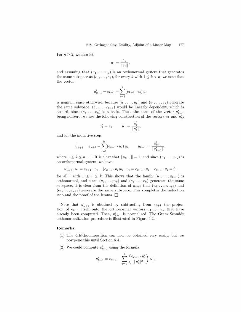
Lemma 6.2.7 Given any nontrivial Euclidean space E of finite dimensionn ≥ 1, from any basis (e1, . . . , en) for E we can construct an orthonormalbasis (u1, . . . , un) for E, with the property that for every k, 1 ≤ k ≤ n, thefamilies (e1, . . . , ek) and (u1, . . . , uk) generate the same subspace.
Proof . We proceed by induction on n. For n = 1, let
u1 =e1‖e1‖
.
6.2. Orthogonality, Duality, Adjoint of a Linear Map 177
For n ≥ 2, we also let
u1 =e1‖e1‖
,
and assuming that (u1, . . . , uk) is an orthonormal system that generatesthe same subspace as (e1, . . . , ek), for every k with 1 ≤ k < n, we note thatthe vector
u′k+1 = ek+1 −k∑
i=1
(ek+1 · ui)ui
is nonnull, since otherwise, because (u1, . . . , uk) and (e1, . . . , ek) generatethe same subspace, (e1, . . . , ek+1) would be linearly dependent, which isabsurd, since (e1, . . . , en) is a basis. Thus, the norm of the vector u′k+1
being nonzero, we use the following construction of the vectors uk and u′k:
u′1 = e1, u1 =u′1‖u′1‖
,
and for the inductive step
u′k+1 = ek+1 −k∑
i=1
(ek+1 · ui)ui, uk+1 =u′k+1
‖u′k+1‖,
where 1 ≤ k ≤ n− 1. It is clear that ‖uk+1‖ = 1, and since (u1, . . . , uk) isan orthonormal system, we have
u′k+1 · ui = ek+1 · ui − (ek+1 · ui)ui · ui = ek+1 · ui − ek+1 · ui = 0,
for all i with 1 ≤ i ≤ k. This shows that the family (u1, . . . , uk+1) isorthonormal, and since (u1, . . . , uk) and (e1, . . . , ek) generates the samesubspace, it is clear from the definition of uk+1 that (u1, . . . , uk+1) and(e1, . . . , ek+1) generate the same subspace. This completes the inductionstep and the proof of the lemma.
Note that u′k+1 is obtained by subtracting from ek+1 the projec-tion of ek+1 itself onto the orthonormal vectors u1, . . . , uk that havealready been computed. Then, u′k+1 is normalized. The Gram–Schmidtorthonormalization procedure is illustrated in Figure 6.2.
Remarks:
(1) The QR-decomposition can now be obtained very easily, but wepostpone this until Section 6.4.
(2) We could compute u′k+1 using the formula
u′k+1 = ek+1 −k∑
i=1
(ek+1 · u′i‖u′i‖2
)u′i,
178 6. Basics of Euclidean Geometry
e1e2
e3
u1
(e2 · u1)u1
(e3 · u1)u1
(e3 · u2)u2u2 u′2
u3
u′3
Figure 6.2. The Gram–Schmidt orthonormalization procedure
and normalize the vectors u′k at the end. This time, we are sub-tracting from ek+1 the projection of ek+1 itself onto the orthogonalvectors u′1, . . . , u
′k. This might be preferable when writing a computer
program.
(3) The proof of Lemma 6.2.7 also works for a countably infinite basisfor E, producing a countably infinite orthonormal basis.
Example 6.5 If we consider polynomials and the inner product
〈f, g〉 =
∫ 1
−1
f(t)g(t)dt,
applying the Gram–Schmidt orthonormalization procedure to the polyno-mials
1, x, x2, . . . , xn, . . . ,
which form a basis of the polynomials in one variable with real coefficients,we get a family of orthonormal polynomials Qn(x) related to the Legendrepolynomials.
The Legendre polynomials Pn(x) have many nice properties. They areorthogonal, but their norm is not always 1. The Legendre polynomialsPn(x) can be defined as follows. Letting fn be the function
fn(x) = (x2 − 1)n,
we define Pn(x) as follows:
P0(x) = 1, and Pn(x) =1
2nn!f (n)
n (x),
6.2. Orthogonality, Duality, Adjoint of a Linear Map 179
where f(n)n is the nth derivative of fn.
They can also be defined inductively as follows:
P0(x) = 1,
P1(x) = x,
Pn+1(x) =2n+ 1
n+ 1xPn(x) − n
n+ 1Pn−1(x).
It turns out that the polynomials Qn are related to the Legendrepolynomials Pn as follows:
Qn(x) =2n(n!)2
(2n)!Pn(x).
As a consequence of Lemma 6.2.6 (or Lemma 6.2.7), given any Euclideanspace of finite dimension n, if (e1, . . . , en) is an orthonormal basis for E,then for any two vectors u = u1e1 + · · · + unen and v = v1e1 + · · · + vnen,the inner product u · v is expressed as
u · v = (u1e1 + · · · + unen) · (v1e1 + · · · + vnen) =
n∑
i=1
uivi,
and the norm ‖u‖ as
‖u‖ = ‖u1e1 + · · · + unen‖ =
√√√√n∑
i=1
u2i .
We can also prove the following lemma regarding orthogonal spaces.
Lemma 6.2.8 Given any nontrivial Euclidean space E of finite dimensionn ≥ 1, for any subspace F of dimension k, the orthogonal complementF⊥ of F has dimension n − k, and E = F ⊕ F⊥. Furthermore, we haveF⊥⊥ = F .
Proof . From Lemma 6.2.6, the subspace F has some orthonormal basis(u1, . . . , uk). This linearly independent family (u1, . . . , uk) can be extendedto a basis (u1, . . . , uk, vk+1, . . . , vn), and by Lemma 6.2.7, it can be con-verted to an orthonormal basis (u1, . . . , un), which contains (u1, . . . , uk) asan orthonormal basis of F . Now, any vector w = w1u1 + · · ·+wnun ∈ E isorthogonal to F iff w · ui = 0, for every i, where 1 ≤ i ≤ k, iff wi = 0 forevery i, where 1 ≤ i ≤ k. Clearly, this shows that (uk+1, . . . , un) is a basisof F⊥, and thus E = F ⊕F⊥, and F⊥ has dimension n− k. Similarly, anyvector w = w1u1 + · · · + wnun ∈ E is orthogonal to F⊥ iff w · ui = 0, forevery i, where k + 1 ≤ i ≤ n, iff wi = 0 for every i, where k + 1 ≤ i ≤ n.Thus, (u1, . . . , uk) is a basis of F⊥⊥, and F⊥⊥ = F .
We now define Euclidean affine spaces.
Definition 6.2.9 An affine space(E,
−→E)
is a Euclidean affine space if
its underlying vector space−→E is a Euclidean vector space. Given any two
180 6. Basics of Euclidean Geometry
points a, b ∈ E, we define the distance between a and b, or length of thesegment (a, b), as ‖ab‖, the Euclidean norm of ab. Given any two pairs ofpoints (a, b) and (c, d), we define their inner product as ab ·cd. We say that(a, b) and (c, d) are orthogonal, or perpendicular , if ab · cd = 0. We saythat two affine subspaces F1 and F2 of E are orthogonal if their directionsF1 and F2 are orthogonal.
The verification that the distance defined in Definition 6.2.9 satisfies theaxioms of Definition 17.2.1 is immediate. Note that a Euclidean affine spaceis a normed affine space, in the sense of Definition 17.2.3. We denote by E
m
the Euclidean affine space obtained from the affine space Am by defining
on the vector space Rm the standard inner product
(x1, . . . , xm) · (y1, . . . , ym) = x1y1 + · · · + xmym.
The corresponding Euclidean norm is
‖(x1, . . . , xm)‖ =√x2
1 + · · · + x2m.
6.3 Linear Isometries (OrthogonalTransformations)
In this section we consider linear maps between Euclidean spaces that pre-serve the Euclidean norm. These transformations, sometimes called rigidmotions, play an important role in geometry.
Definition 6.3.1 Given any two nontrivial Euclidean spaces E and Fof the same finite dimension n, a function f :E → F is an orthogonaltransformation, or a linear isometry , if it is linear and
‖f(u)‖ = ‖u‖,for all u ∈ E.
Remarks:
(1) A linear isometry is often defined as a linear map such that
‖f(v) − f(u)‖ = ‖v − u‖,for all u, v ∈ E. Since the map f is linear, the two definitionsare equivalent. The second definition just focuses on preserving thedistance between vectors.
(2) Sometimes, a linear map satisfying the condition of Definition 6.3.1is called a metric map, and a linear isometry is defined as a bijectivemetric map.
6.3. Linear Isometries (Orthogonal Transformations) 181
An isometry (without the word linear) is sometimes defined as a functionf :E → F (not necessarily linear) such that
‖f(v) − f(u)‖ = ‖v − u‖,for all u, v ∈ E, i.e., as a function that preserves the distance. This require-ment turns out to be very strong. Indeed, the next lemma shows that allthese definitions are equivalent when E and F are of finite dimension, andfor functions such that f(0) = 0.
Lemma 6.3.2 Given any two nontrivial Euclidean spaces E and F ofthe same finite dimension n, for every function f :E → F , the followingproperties are equivalent:
(1) f is a linear map and ‖f(u)‖ = ‖u‖, for all u ∈ E;
(2) ‖f(v) − f(u)‖ = ‖v − u‖, for all u, v ∈ E, and f(0) = 0;
(3) f(u) · f(v) = u · v, for all u, v ∈ E.
Furthermore, such a map is bijective.
Proof . Clearly, (1) implies (2), since in (1) it is assumed that f is linear.Assume that (2) holds. In fact, we shall prove a slightly stronger result.
We prove that if
‖f(v) − f(u)‖ = ‖v − u‖for all u, v ∈ E, then for any vector τ ∈ E, the function g:E → F definedsuch that
g(u) = f(τ + u) − f(τ)
for all u ∈ E is a linear map such that g(0) = 0 and (3) holds. Clearly,g(0) = f(τ) − f(τ) = 0.
Note that from the hypothesis
‖f(v) − f(u)‖ = ‖v − u‖for all u, v ∈ E, we conclude that
‖g(v) − g(u)‖ = ‖f(τ + v) − f(τ) − (f(τ + u) − f(τ))‖,= ‖f(τ + v) − f(τ + u)‖,= ‖τ + v − (τ + u)‖,= ‖v − u‖,
for all u, v ∈ E. Since g(0) = 0, by setting u = 0 in
‖g(v) − g(u)‖ = ‖v − u‖,we get
‖g(v)‖ = ‖v‖
182 6. Basics of Euclidean Geometry
for all v ∈ E. In other words, g preserves both the distance and the norm.To prove that g preserves the inner product, we use the simple fact that
2u · v = ‖u‖2 + ‖v‖2 − ‖u− v‖2
for all u, v ∈ E. Then, since g preserves distance and norm, we have
2g(u) · g(v) = ‖g(u)‖2 + ‖g(v)‖2 − ‖g(u) − g(v)‖2
= ‖u‖2 + ‖v‖2 − ‖u− v‖2
= 2u · v,and thus g(u) · g(v) = u · v, for all u, v ∈ E, which is (3).
In particular, if f(0) = 0, by letting τ = 0, we have g = f , and fpreserves the scalar product, i.e., (3) holds.
Now assume that (3) holds. Since E is of finite dimension, we can pickan orthonormal basis (e1, . . . , en) for E. Since f preserves inner products,(f(e1), . . . , f(en)) is also orthonormal, and since F also has dimension n,it is a basis of F . Then note that for any u = u1e1 + · · · + unen, we have
ui = u · ei,
for all i, 1 ≤ i ≤ n. Thus, we have
f(u) =
n∑
i=1
(f(u) · f(ei))f(ei),
and since f preserves inner products, this shows that
f(u) =
n∑
i=1
(u · ei)f(ei) =
n∑
i=1
uif(ei),
which shows that f is linear. Obviously, f preserves the Euclidean norm,and (3) implies (1).
Finally, if f(u) = f(v), then by linearity f(v−u) = 0, so that ‖f(v−u)‖= 0, and since f preserves norms, we must have ‖v−u‖ = 0, and thus u = v.Thus, f is injective, and since E and F have the same finite dimension, fis bijective.
Remarks:
(i) The dimension assumption is needed only to prove that (3) implies(1) when f is not known to be linear, and to prove that f is surjective,but the proof shows that (1) implies that f is injective.
(ii) In (2), when f does not satisfy the condition f(0) = 0, the proofshows that f is an affine map. Indeed, taking any vector τ as anorigin, the map g is linear, and
f(τ + u) = f(τ) + g(u)
for all u ∈ E, proving that f is affine with associated linear map g.
6.4. The Orthogonal Group, Orthogonal Matrices 183
(iii) Paul Hughett showed me a nice proof of the following interesting fact:The implication that (3) implies (1) holds if we also assume that f issurjective, even if E has infinite dimension. Indeed, observe that
(f(λu+ µv) − λf(u) − µf(v)) · f(w)
= f(λu+ µv) · f(w) − λf(u) · f(w) − µf(v) · f(w)
= (λu+ µv) · w − λu · w − µv · w = 0,
since f preserves the inner product. However, if f is surjective, everyz ∈ E is of the form z = f(w) for some w ∈ E, and the aboveequation implies that
(f(λu+ µv) − λf(u) − µf(v)) · z = 0
for all z ∈ E, which implies that
f(λu+ µv) − λf(u) − µf(v) = 0,
proving that f is linear.
In view of Lemma 6.3.2, we will drop the word “linear” in “linear isome-try,” unless we wish to emphasize that we are dealing with a map betweenvector spaces.
We are now going to take a closer look at the isometries f :E → E of aEuclidean space of finite dimension.
6.4 The Orthogonal Group, Orthogonal Matrices
In this section we explore some of the basic properties of the orthogonalgroup and of orthogonal matrices.
Lemma 6.4.1 Let E be any Euclidean space of finite dimension n, and letf :E → E be any linear map. The following properties hold:
(1) The linear map f :E → E is an isometry iff
f f∗ = f∗ f = id.
(2) For every orthonormal basis (e1, . . . , en) of E, if the matrix of f is A,then the matrix of f∗ is the transpose A> of A, and f is an isometryiff A satisfies the identities
AA> = A>A = In,
where In denotes the identity matrix of order n, iff the columnsof A form an orthonormal basis of E, iff the rows of A form anorthonormal basis of E.
184 6. Basics of Euclidean Geometry
Proof . (1) The linear map f :E → E is an isometry iff
f(u) · f(v) = u · v,for all u, v ∈ E, iff
f∗(f(u)) · v = f(u) · f(v) = u · vfor all u, v ∈ E, which implies
(f∗(f(u)) − u) · v = 0
for all u, v ∈ E. Since the inner product is positive definite, we must have
f∗(f(u)) − u = 0
for all u ∈ E, that is,
f∗ f = f f∗ = id.
(2) If (e1, . . . , en) is an orthonormal basis for E, let A = (ai,j) be thematrix of f , and let B = (bi,j) be the matrix of f∗. Since f∗ is characterizedby
f∗(u) · v = u · f(v)
for all u, v ∈ E, using the fact that if w = w1e1 + · · · + wnen we havewk = w · ek for all k, 1 ≤ k ≤ n, letting u = ei and v = ej , we get
bj,i = f∗(ei) · ej = ei · f(ej) = ai,j ,
for all i, j, 1 ≤ i, j ≤ n. Thus, B = A>. Now, if X and Y are arbitrarymatrices over the basis (e1, . . . , en), denoting as usual the jth column of Xby Xj , and similarly for Y , a simple calculation shows that
X>Y = (Xi · Yj)1≤i,j≤n.
Then it is immediately verified that if X = Y = A, then
A>A = AA> = In
iff the column vectors (A1, . . . , An) form an orthonormal basis. Thus, from(1), we see that (2) is clear (also because the rows of A are the columns ofA>).
Lemma 6.4.1 shows that the inverse of an isometry f is its adjoint f ∗.Lemma 6.4.1 also motivates the following definition. The set of all real n×nmatrices is denoted by Mn(R).
Definition 6.4.2 A real n× n matrix is an orthogonal matrix if
AA> = A>A = In.
Remark: It is easy to show that the conditions AA> = In, A>A = In, andA−1 = A>, are equivalent. Given any two orthonormal bases (u1, . . . , un)
6.5. QR-Decomposition for Invertible Matrices 185
and (v1, . . . , vn), if P is the change of basis matrix from (u1, . . . , un) to(v1, . . . , vn) (i.e., the columns of P are the coordinates of the vj w.r.t.(u1, . . . , un)), since the columns of P are the coordinates of the vectors vj
with respect to the basis (u1, . . . , un), and since (v1, . . . , vn) is orthonormal,the columns of P are orthonormal, and by Lemma 6.4.1 (2), the matrix Pis orthogonal.
The proof of Lemma 6.3.2 (3) also shows that if f is an isometry, thenthe image of an orthonormal basis (u1, . . . , un) is an orthonormal basis.Students often ask why orthogonal matrices are not called orthonormalmatrices, since their columns (and rows) are orthonormal bases! I haveno good answer, but isometries do preserve orthogonality, and orthogonalmatrices correspond to isometries.
Recall that the determinant det(f) of a linear map f :E → E is indepen-dent of the choice of a basis in E. Also, for every matrix A ∈ Mn(R), wehave det(A) = det(A>), and for any two n× n matrices A and B, we havedet(AB) = det(A) det(B) (for all these basic results, see Lang [107]). Then,if f is an isometry, and A is its matrix with respect to any orthonormal ba-sis, AA> = A>A = In implies that det(A)2 = 1, that is, either det(A) = 1,or det(A) = −1. It is also clear that the isometries of a Euclidean space ofdimension n form a group, and that the isometries of determinant +1 forma subgroup. This leads to the following definition.
Definition 6.4.3 Given a Euclidean space E of dimension n, the set ofisometries f :E → E forms a subgroup of GL(E) denoted by O(E), orO(n) when E = R
n, called the orthogonal group (of E). For every isometryf , we have det(f) = ±1, where det(f) denotes the determinant of f . Theisometries such that det(f) = 1 are called rotations, or proper isometries, orproper orthogonal transformations, and they form a subgroup of the speciallinear group SL(E) (and of O(E)), denoted by SO(E), or SO(n) whenE = R
n, called the special orthogonal group (of E). The isometries suchthat det(f) = −1 are called improper isometries, or improper orthogonaltransformations, or flip transformations.
As an immediate corollary of the Gram–Schmidt orthonormalizationprocedure, we obtain the QR-decomposition for invertible matrices.
6.5 QR-Decomposition for Invertible Matrices
Now that we have the definition of an orthogonal matrix, we can explainhow the Gram–Schmidt orthonormalization procedure immediately yieldsthe QR-decomposition for matrices.
186 6. Basics of Euclidean Geometry
Lemma 6.5.1 Given any real n×n matrix A, if A is invertible, then thereis an orthogonal matrix Q and an upper triangular matrix R with positivediagonal entries such that A = QR.
Proof . We can view the columns of A as vectors A1, . . . , An in En. If
A is invertible, then they are linearly independent, and we can applyLemma 6.2.7 to produce an orthonormal basis using the Gram–Schmidtorthonormalization procedure. Recall that we construct vectors Qk and Q′
k
as follows:
Q′1 = A1, Q1 =
Q′1
‖Q′1‖,
and for the inductive step
Q′k+1 = Ak+1 −
k∑
i=1
(Ak+1 ·Qi)Qi, Qk+1 =Q′
k+1
‖Q′k+1‖
,
where 1 ≤ k ≤ n− 1. If we express the vectors Ak in terms of the Qi andQ′
i, we get the triangular system
A1 = ‖Q′1‖Q1,
. . .
Aj = (Aj ·Q1)Q1 + · · · + (Aj ·Qi)Qi + · · · + ‖Q′j‖Qj ,
. . .
An = (An ·Q1)Q1 + · · · + (An ·Qn−1)Qn−1 + ‖Q′n‖Qn.
Letting rk,k = ‖Q′k‖, and ri,j = Aj · Qi (the reversal of i and j on
the right-hand side is intentional!), where 1 ≤ k ≤ n, 2 ≤ j ≤ n, and1 ≤ i ≤ j − 1, and letting qi,j be the ith component of Qj , we note thatai,j , the ith component of Aj , is given by
ai,j = r1,jqi,1+· · ·+ri,jqi,i+· · ·+rj,jqi,j = qi,1r1,j+· · ·+qi,iri,j+· · ·+qi,jrj,j .If we let Q = (qi,j), the matrix whose columns are the components ofthe Qj , and R = (ri,j), the above equations show that A = QR, whereR is upper triangular (the reader should work this out on some concreteexamples for 2×2 and 3×3 matrices!). The diagonal entries rk,k = ‖Q′
k‖ =Ak ·Qk are indeed positive.
Remarks:
(1) Because the diagonal entries of R are positive, it can be shown thatQ and R are unique.
(2) The QR-decomposition holds even when A is not invertible. In thiscase, R has some zero on the diagonal. However, a different proof isneeded. We will give a nice proof using Householder matrices (seeLemma 7.3.2, and also Strang [165, 166], Golub and Van Loan [75],Trefethen and Bau [170], Kincaid and Cheney [100], or Ciarlet [33]).
6.5. QR-Decomposition for Invertible Matrices 187
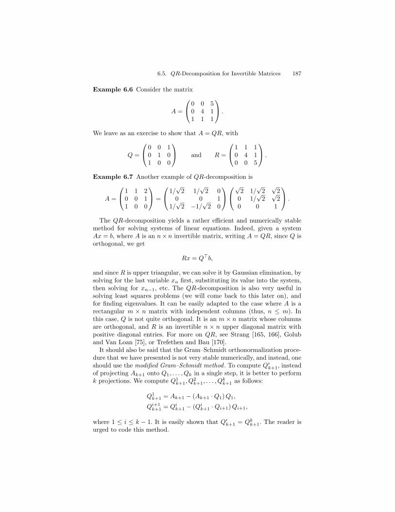
Example 6.6 Consider the matrix
A =
0 0 50 4 11 1 1
.
We leave as an exercise to show that A = QR, with
Q =
0 0 10 1 01 0 0
and R =
1 1 10 4 10 0 5
.
Example 6.7 Another example of QR-decomposition is
A =
1 1 20 0 11 0 0
=
1/√
2 1/√
2 00 0 1
1/√
2 −1/√
2 0
√2 1/
√2
√2
0 1/√
2√
20 0 1
.
The QR-decomposition yields a rather efficient and numerically stablemethod for solving systems of linear equations. Indeed, given a systemAx = b, where A is an n× n invertible matrix, writing A = QR, since Q isorthogonal, we get
Rx = Q>b,
and since R is upper triangular, we can solve it by Gaussian elimination, bysolving for the last variable xn first, substituting its value into the system,then solving for xn−1, etc. The QR-decomposition is also very useful insolving least squares problems (we will come back to this later on), andfor finding eigenvalues. It can be easily adapted to the case where A is arectangular m × n matrix with independent columns (thus, n ≤ m). Inthis case, Q is not quite orthogonal. It is an m× n matrix whose columnsare orthogonal, and R is an invertible n × n upper diagonal matrix withpositive diagonal entries. For more on QR, see Strang [165, 166], Goluband Van Loan [75], or Trefethen and Bau [170].
It should also be said that the Gram–Schmidt orthonormalization proce-dure that we have presented is not very stable numerically, and instead, oneshould use the modified Gram–Schmidt method . To compute Q′
k+1, insteadof projecting Ak+1 onto Q1, . . . , Qk in a single step, it is better to performk projections. We compute Q1
k+1, Q2k+1, . . . , Q
kk+1 as follows:
Q1k+1 = Ak+1 − (Ak+1 ·Q1)Q1,
Qi+1k+1 = Qi
k+1 − (Qik+1 ·Qi+1)Qi+1,
where 1 ≤ i ≤ k − 1. It is easily shown that Q′k+1 = Qk
k+1. The reader isurged to code this method.
188 6. Basics of Euclidean Geometry
6.6 Some Applications of Euclidean Geometry
Euclidean geometry has applications in computational geometry, in partic-ular Voronoi diagrams and Delaunay triangulations, discussed in Chapter9. In turn, Voronoi diagrams have applications in motion planning (seeO’Rourke [132]).
Euclidean geometry also has applications to matrix analysis. Recall thata real n× n matrix A is symmetric if it is equal to its transpose A>. Oneof the most important properties of symmetric matrices is that they havereal eigenvalues and that they can be diagonalized by an orthogonal matrix(see Chapter 11). This means that for every symmetric matrix A, there isa diagonal matrix D and an orthogonal matrix P such that
A = PDP>.
Even though it is not always possible to diagonalize an arbitrary matrix,there are various decompositions involving orthogonal matrices that are ofgreat practical interest. For example, for every real matrix A, there is theQR-decomposition, which says that a real matrix A can be expressed as
A = QR,
where Q is orthogonal and R is an upper triangular matrix. This can beobtained from the Gram–Schmidt orthonormalization procedure, as we sawin Section 6.5, or better, using Householder matrices, as shown in Section7.3. There is also the polar decomposition, which says that a real matrix Acan be expressed as
A = QS,
where Q is orthogonal and S is symmetric positive semidefinite (whichmeans that the eigenvalues of S are nonnegative; see Chapter 11). Such adecomposition is important in continuum mechanics and in robotics, sinceit separates stretching from rotation. Finally, there is the wonderful singularvalue decomposition, abbreviated as SVD, which says that a real matrix Acan be expressed as
A = V DU>,
where U and V are orthogonal and D is a diagonal matrix with nonneg-ative entries (see Chapter 12). This decomposition leads to the notion ofpseudo-inverse, which has many applications in engineering (least squaressolutions, etc). For an excellent presentation of all these notions, we highlyrecommend Strang [166, 165], Golub and Van Loan [75], and Trefethen andBau [170].
The method of least squares, invented by Gauss and Legendre around1800, is another great application of Euclidean geometry. Roughly speaking,the method is used to solve inconsistent linear systems Ax = b, where thenumber of equations is greater than the number of variables. Since this
6.7. Problems 189
is generally impossible, the method of least squares consists in finding asolution x minimizing the Euclidean norm ‖Ax − b‖2, that is, the sumof the squares of the “errors.” It turns out that there is always a uniquesolution x+ of smallest norm minimizing ‖Ax−b‖2, and that it is a solutionof the square system
A>Ax = A>b,
called the system of normal equations. The solution x+ can be found eitherby using the QR-decomposition in terms of Householder transformations,or by using the notion of pseudo-inverse of a matrix. The pseudo-inversecan be computed using the SVD decomposition. Least squares methods areused extensively in computer vision; see Trucco and Verri [171], or Jain,Katsuri, and Schunck [93]. More details on the method of least squares andpseudo-inverses can be found in Section 13.1.
6.7 Problems
Problem 6.1 Prove Lemma 6.2.2.
Problem 6.2 Prove Lemma 6.2.3.
Problem 6.3 Let (e1, . . . , en) be an orthonormal basis for E. If X and Yare arbitrary n×n matrices, denoting as usual the jth column of X by Xj ,and similarly for Y , show that
X>Y = (Xi · Yj)1≤i,j≤n.
Use this to prove that
A>A = AA> = In
iff the column vectors (A1, . . . , An) form an orthonormal basis. Show thatthe conditions AA> = In, A>A = In, and A−1 = A> are equivalent.
Problem 6.4 Given any two linear maps f :E → F and g:F → E, wheredim(E) = n and dim(F ) = m, prove that
(−λ)m det(g f − λ In) = (−λ)n det(f g − λ Im),
and thus that g f and f g have the same nonnull eigenvalues.Hint . If A is an m× n matrix and B is an n×m matrix, observe that
∣∣∣∣AB −X Im 0m,n
B −X In
∣∣∣∣ =
∣∣∣∣A XImIn 0n,m
∣∣∣∣∣∣∣∣B −XIn
−Im A
∣∣∣∣
and ∣∣∣∣A XImIn 0n,m
∣∣∣∣∣∣∣∣B −XIn
−Im A
∣∣∣∣ =
∣∣∣∣BA−X In XB
0m,n −X Im
∣∣∣∣ ,
where X is a variable.
190 6. Basics of Euclidean Geometry
Problem 6.5 (a) Let C1 = (C1, R1) and C2 = (C2, R2) be two distinctcircles in the plane E
2 (where Ci is the center and Ri is the radius). Whatis the locus of the centers of all circles tangent to both C1 and C2?Hint . When is it one conic, when is it two conics?
(b) Repeat question (a) in the case where C2 is a line.(c) Given three pairwise distinct circles C1 = (C1, R1), C2 = (C2, R2), and
C3 = (C3, R3) in the plane E2, prove that there are at most eight circles
simultaneously tangent to C1, C2, and C3 (this is known as the problemof Apollonius). What happens if the centers C1, C2, C3 of the circles arecollinear? In the latter case, show that there are at most two circles exteriorand tangent to C1, C2, and C3.Hint . You may want to use a carefully chosen inversion (see the problemsin Section 5.14, especially Problem 5.37).
(d) Prove that the problem of question (c) reduces to the problem of find-ing the circles passing through a fixed point and tangent to two given circles.In turn, by inversion, this problem reduces to finding all lines tangent totwo circles.
(e) Given four pairwise distinct spheres C1 = (C1, R1), C2 = (C2, R2),C3 = (C3, R3), and C4 = (C4, R4), prove that there are at most sixteenspheres simultaneously tangent to C1, C2, C3, and C4. Prove that this prob-lem reduces to the problem of finding the spheres passing through a fixedpoint and tangent to three given spheres. In turn, by inversion, this problemreduces to finding all planes tangent to three spheres.
Problem 6.6 (a) Given any two circles C1 and C2 in E2 of equations
x2 + y2 − 2ax− 2by + c = 0 and x2 + y2 − 2a′x− 2′by + c′ = 0,
we say that C1 and C2 are orthogonal if they intersect and if the tangents atthe intersection points are orthogonal. Prove that C1 and C2 are orthogonaliff
2(aa′ + bb′) = c+ c′.
(b) For any given c ∈ R (c 6= 0), there is a pencil F of circles of equations
x2 + y2 − 2ux− c = 0,
where u ∈ R is arbitrary. Show that the set of circles orthogonal to allcircles in the pencil F is the pencil F⊥ of circles of equations
x2 + y2 − 2vy + c = 0,
where v ∈ R is arbitrary.
Problem 6.7 Let P = p1, . . . , pn be a finite set of points in E3. Show
that there is a unique point c such that the sum of the squares of thedistances from c to each pi is minimal. Find this point in terms of the pi.
6.7. Problems 191
Problem 6.8 (1) Compute the real Fourier coefficients of the functionid(x) = x over [−π, π] and prove that
x = 2
(sinx
1− sin 2x
2+
sin 3x
3− · · ·
).
What is the value of the Fourier series at ±π? What is the value of theFourier near ±π? Do you find this surprising?
(2) Plot the functions obtained by keeping 1, 2, 4, 5, and 10 terms. Whatdo you observe around ±π?
Problem 6.9 The Dirac delta function (which is not a function!) is thespike function s.t. δ(k2π) = +∞ for all k ∈ Z, and δ(x) = 0 everywhereelse. It has the property that for “well-behaved” functions f (includingconstant functions and trigonometric functions),
∫ +π
−π
f(t)δ(t)dt = f(0).
(1) Compute the real Fourier coefficients of δ over [−π, π], and prove that
δ(x) =1
2π(1 + 2 cosx+ 2 cos 2x+ 2 cos 3x+ · · · + 2 cosnx+ · · ·) .
Also compute the complex Fourier coefficients of δ over [−π, π], and provethat
δ(x) =1
2π
(1 + eix + e−ix + ei2x + e−i2x + · · · + einx + e−inx + · · ·
).
(2) Prove that the partial sum of the first 2n+ 1 complex terms is
δn(x) =sin ((2n+ 1)(x/2))
2π sin (x/2).
What is δn(0)?(3) Plot δn(x) for n = 10, 20 (over [−π, π]). Prove that the area under
the curve δn is independent of n. What is it?
Problem 6.10 (1) If an upper triangular n × n matrix R is invertible,prove that its inverse is also upper triangular.
(2) If an upper triangular matrix is orthogonal, prove that it must be adiagonal matrix.
If A is an invertible n × n matrix and if A = Q1R1 = Q2R2, where R1
and R2 are upper triangular with positive diagonal entries and Q1, Q2 areorthogonal, prove that Q1 = Q2 and R1 = R2.
Problem 6.11 (1) Review the modified Gram–Schmidt method. Recallthat to compute Q′
k+1, instead of projecting Ak+1 onto Q1, . . . , Qk in a sin-gle step, it is better to perform k projections. We compute Q1
k+1, Q2k+1, . . .,
Qkk+1 as follows:
Q1k+1 = Ak+1 − (Ak+1 ·Q1)Q1,
192 6. Basics of Euclidean Geometry
Qi+1k+1 = Qi
k+1 − (Qik+1 ·Qi+1)Qi+1,
where 1 ≤ i ≤ k − 1.Prove that Q′
k+1 = Qkk+1.
(2) Write two computer programs to compute the QR-decomposition ofan invertible matrix. The first one should use the standard Gram–Schmidtmethod, and the second one the modified Gram–Schmidt method. Runboth on a number of matrices, up to dimension at least 10. Do you observeany difference in their performance in terms of numerical stability?
Run your programs on the Hilbert matrix Hn = (1/(i + j − 1))1≤i,j≤n.What happens?
Extra Credit. Write a program to solve linear systems of equationsAx = b, using your version of the QR-decomposition program, where A isan n× n matrix.
Problem 6.12 Let E be a Euclidean space of finite dimension n, and let(e1, . . . , en) be an orthonormal basis for E. For any two vectors u, v ∈ E,the linear map u⊗ v is defined such that
u⊗ v(x) = (v · x)u,for all x ∈ E. If U and V are the column vectors of coordinates of u and vw.r.t. the basis (e1, . . . , en), prove that u⊗ v is represented by the matrix
U>V.
What sort of linear map is u⊗ u when u is a unit vector?
Problem 6.13 Let ϕ:E×E → R be a bilinear form on a real vector spaceE of finite dimension n. Given any basis (e1, . . . , en) of E, let A = (αi j)be the matrix defined such that
αi j = ϕ(ei, ej),
1 ≤ i, j ≤ n. We call A the matrix of ϕ w.r.t. the basis (e1, . . . , en).(a) For any two vectors x and y, if X and Y denote the column vectors
of coordinates of x and y w.r.t. the basis (e1, . . . , en), prove that
ϕ(x, y) = X>AY.
(b) Recall that A is a symmetric matrix if A = A>. Prove that ϕ issymmetric if A is a symmetric matrix.
(c) If (f1, . . . , fn) is another basis of E and P is the change of basismatrix from (e1, . . . , en) to (f1, . . . , fn), prove that the matrix of ϕ w.r.t.the basis (f1, . . . , fn) is
P>AP.
The common rank of all matrices representing ϕ is called the rank of ϕ.
Problem 6.14 Let ϕ:E × E → R be a symmetric bilinear form on a realvector space E of finite dimension n. Two vectors x and y are said to be
6.7. Problems 193
conjugate w.r.t. ϕ if ϕ(x, y) = 0. The main purpose of this problem is toprove that there is a basis of vectors that are pairwise conjugate w.r.t. ϕ.
(a) Prove that if ϕ(x, x) = 0 for all x ∈ E, then ϕ is identically null onE.
Otherwise, we can assume that there is some vector x ∈ E such thatϕ(x, x) 6= 0. Use induction to prove that there is a basis of vectors that arepairwise conjugate w.r.t. ϕ.
For the induction step, proceed as follows. Let (e1, e2, . . . , en) be a basisof E, with ϕ(e1, e1) 6= 0. Prove that there are scalars λ2, . . . , λn such thateach of the vectors
vi = ei + λie1
is conjugate to e1 w.r.t. ϕ, where 2 ≤ i ≤ n, and that (e1, v2, . . . , vn) is abasis.
(b) Let (e1, . . . , en) be a basis of vectors that are pairwise conjugate w.r.t.ϕ, and assume that they are ordered such that
ϕ(ei, ei) =
θi 6= 0 if 1 ≤ i ≤ r,0 if r + 1 ≤ i ≤ n,
where r is the rank of ϕ. Show that the matrix of ϕ w.r.t. (e1, . . . , en) is adiagonal matrix, and that
ϕ(x, y) =
r∑
i=1
θixiyi,
where x =∑n
i=1 xiei and y =∑n
i=1 yiei.Prove that for every symmetric matrix A, there is an invertible matrix
P such that
P>AP = D,
where D is a diagonal matrix.(c) Prove that there is an integer p, 0 ≤ p ≤ r (where r is the rank of ϕ),
such that ϕ(ui, ui) > 0 for exactly p vectors of every basis (u1, . . . , un) ofvectors that are pairwise conjugate w.r.t. ϕ (Sylvester’s inertia theorem).
Proceed as follows. Assume that in the basis (u1, . . . , un), for any x ∈ E,we have
ϕ(x, x) = α1x21 + · · · + αpx
2p − αp+1x
2p+1 − · · · − αrx
2r,
where x =∑n
i=1 xiui, and that in the basis (v1, . . . , vn), for any x ∈ E, wehave
ϕ(x, x) = β1y21 + · · · + βqy
2q − βq+1y
2q+1 − · · · − βry
2r ,
where x =∑n
i=1 yivi, with αi > 0, βi > 0, 1 ≤ i ≤ r.Assume that p > q and derive a contradiction. First, consider x in the
subspace F spanned by
(u1, . . . , up, ur+1, . . . , un),
194 6. Basics of Euclidean Geometry
and observe that ϕ(x, x) ≥ 0 if x 6= 0. Next, consider x in the subspace Gspanned by
(vq+1, . . . , vr),
and observe that ϕ(x, x) < 0 if x 6= 0. Prove that F ∩G is nontrivial (i.e.,contains some nonnull vector), and derive a contradiction. This implies thatp ≤ q. Finish the proof.
The pair (p, r − p) is called the signature of ϕ.(d) A symmetric bilinear form ϕ is definite if for every x ∈ E, if ϕ(x, x) =
0, then x = 0.Prove that a symmetric bilinear form is definite iff its signature is either
(n, 0) or (0, n). In other words, a symmetric definite bilinear form has rankn and is either positive or negative.
(e) The kernel of a symmetric bilinear form ϕ is the subspace consisting ofthe vectors that are conjugate to all vectors in E. We say that a symmetricbilinear form ϕ is nondegenerate if its kernel is trivial (i.e., equal to 0).
Prove that a symmetric bilinear form ϕ is nondegenerate iff its rank is n,the dimension of E. Is a definite symmetric bilinear form ϕ nondegenerate?What about the converse?
Prove that if ϕ is nondegenerate, then there is a basis of vectors that arepairwise conjugate w.r.t. ϕ and such that ϕ is represented by the matrix
(Ip 00 −Iq
)
where (p, q) is the signature of ϕ.(f) Given a nondegenerate symmetric bilinear form ϕ on E, prove that
for every linear map f :E → E, there is a unique linear map f ∗:E → Esuch that
ϕ(f(u), v) = ϕ(u, f∗(v)),
for all u, v ∈ E. The map f∗ is called the adjoint of f (w.r.t. to ϕ). Givenany basis (u1, . . . , un), if Ω is the matrix representing ϕ and A is the matrixrepresenting f , prove that f∗ is represented by Ω−1A>Ω.
Prove that Lemma 6.2.4 also holds, i.e., the map [:E → E∗ is a canonicalisomorphism.
A linear map f :E → E is an isometry w.r.t. ϕ if
ϕ(f(x), f(y)) = ϕ(x, y)
for all x, y ∈ E. Prove that a linear map f is an isometry w.r.t. ϕ iff
f∗ f = f f∗ = id.
Prove that the set of isometries w.r.t. ϕ is a group. This group is denotedby O(ϕ), and its subgroup consisting of isometries having determinant +1by SO(ϕ). Given any basis of E, if Ω is the matrix representing ϕ and A
6.7. Problems 195
is the matrix representing f , prove that f ∈ O(ϕ) iff
A>ΩA = Ω.
Given another nondegenerate symmetric bilinear form ψ on E, we saythat ϕ and ψ are equivalent if there is a bijective linear map h:E → Esuch that
ψ(x, y) = ϕ(h(x), h(y)),
for all x, y ∈ E. Prove that the groups of isometries O(ϕ) and O(ψ) areisomomorphic (use the map f 7→ h f h−1 from O(ψ) to O(ϕ)).
If ϕ is a nondegenerate symmetric bilinear form of signature (p, q), provethat the group O(ϕ) is isomorphic to the group of n × n matrices A suchthat
A>
(Ip 00 −Iq
)A =
(Ip 00 −Iq
).
Remark: In view of question (f), the groups O(ϕ) and SO(ϕ) are alsodenoted by O(p, q) and SO(p, q) when ϕ has signature (p, q). They areLie groups. In particular, the group SO(3, 1), known as the Lorentz group,plays an important role in the theory of special relativity.
Problem 6.15 (a) Let C be a circle of radius R and center O, and let Pbe any point in the Euclidean plane E
2. Consider the lines ∆ through Pthat intersect the circle C, generally in two points A and B. Prove that forall such lines,
PA · PB = ‖PO‖2 −R2.
Hint . If P is not on C, let B′ be the antipodal of B (i.e., OB′ = −OB).Then AB · AB′ = 0 and
PA · PB = PB′ · PB = (PO − OB) · (PO + OB) = ‖PO‖2 −R2.
The quantity ‖PO‖2 − R2 is called the power of P w.r.t. C, and it isdenoted by P(P,C).
Show that if ∆ is tangent to C, then A = B and
‖PA‖2 = ‖PO‖2 −R2.
Show that P is inside C iff P(P,C) < 0, on C iff P(P,C) = 0, outsideC if P(P,C) > 0.
If the equation of C is
x2 + y2 − 2ax− 2by + c = 0,
prove that the power of P = (x, y) w.r.t. C is given by
P(P,C) = x2 + y2 − 2ax− 2by + c.
196 6. Basics of Euclidean Geometry
(b) Given two nonconcentric circles C and C ′, show that the set of pointshaving equal power w.r.t. C and C ′ is a line orthogonal to the line throughthe centers of C and C ′. If the equations of C and C ′ are
x2 + y2 − 2ax− 2by + c = 0 and x2 + y2 − 2a′x− 2b′y + c′ = 0,
show that the equation of this line is
2(a− a′)x+ 2(b− b′)y + c′ − c = 0.
This line is called the radical axis of C and C ′.(c) Given three distinct nonconcentric circles C, C ′, and C ′′, prove that
either the three pairwise radical axes of these circles are parallel or thatthey intersect in a single point ω that has equal power w.r.t. C, C ′, and C ′′.In the first case, the centers of C, C ′, and C ′′ are collinear. In the secondcase, if the power of ω is positive, prove that ω is the center of a circle Γorthogonal to C, C ′, and C ′′, and if the power of ω is negative, ω is insideC, C ′, and C ′′.
(d) Given any k ∈ R with k 6= 0 and any point a, recall that an inversionof pole a and power k is a map h: (En − a) → E
n defined such that forevery x ∈ E
n − a,
h(x) = a+ kax
‖ax‖2.
For example, when n = 2, chosing any orthonormal frame with origin a, his defined by the map
(x, y) 7→(
kx
x2 + y2,
ky
x2 + y2
).
When the centers of C, C ′ and C ′′ are not collinear and the power of ω ispositive, prove that by a suitable inversion, C, C ′ and C ′′ are mapped tothree circles whose centers are collinear.
Prove that if three distinct nonconcentric circles C, C ′, and C ′′ havecollinear centers, then there are at most eight circles simultaneously tangentto C, C ′, and C ′′, and at most two for those exterior to C, C ′, and C ′′.
(e) Prove that an inversion in E3 maps a sphere to a sphere or to a plane.
Prove that inversions preserve tangency and orthogonality of planes andspheres.