Embed Size (px)
Citation preview

Chapter 1
Basics of Probability
1.1 Introduction
1.2 Basic Concepts and Definitions
1.2.1 Sample space = {TTT, TTH, THT, HTT, THH, HTH, HHT, HHH},
A = {TTT, TTH, THT, HTT, THH, HTH, HHT},
P (A) = 7/8
1.2.2 The sample space is given in the table below:
RRRR RRRL RRLR RLRR LRRR
RRLL RLRL RLLR LLRR LRRL
LRLR RLLL LRLL LLRL LLLR
LLLL
From the sample space, we see there are 6 outcomes where exactly 2 cars turn left. Assumingeach outcome is equally likely, the probability that exactly 2 cars turn left is 6/16 = 3/8. Thisassumption is probably not very reasonable since at a given intersection, cars typically turn onedirection more often than the other.
1.2.3
1

2 CHAPTER 1 Basics of Probability
a. Since there are 365 days in a year and exactly one day is the person’s birthday, the probabilityof guessing correctly is 1/365.
b. By similar reasoning as part a., the probability of guessing the correct month is 1/12.
1.2.4
a. The sample space is given in the table below:
Die
Coin 1 2 3 4 5 6
T 1T 2T 3T 4T 5T 6T
H 1H 2H 3H 4H 5H 6H
b. The event of getting a tail and at least a 5 is A = {5T, 6T} and P (A) = 2/12 = 1/6
1.2.5
a. P (X ! 3) = 3!(!2)5!(!2) =
57
b. P (X " #1.5) = 3!(!1.5)5!(!2) = 6.5
7
c. P (#1 ! X ! 4) = 4!(!1)5!(!2) =
57
d. P (0 ! X ! 6) = 5!05!(!2) =
57
e. P (X " 4) = 5!45!(!2) =
17
f. P (X = #0.75) = 0
1.2.6
a. The sample space is given in the table below:
1 2 3 4 5 6
1 1 2 3 4 5 6
2 2 4 6 8 10 12
3 3 6 9 12 15 18
4 4 8 12 16 20 24
5 5 10 15 20 25 30
6 6 12 18 24 30 36
b. The distribution of the product is given in the table below:
x 1 2 3 4 5 6 8 9 10 12 15 16 18 20 24 25 30 36
# of Outcomes 1 2 2 3 2 4 2 1 2 4 2 1 2 2 2 1 2 1
P (x) 136
118
118
112
118
19
118
136
118
19
118
136
118
118
118
136
118
136
1.3 Counting Problems 3
c. P (5 ! X ! 25) = P (X = 5) + · · ·+ P (X = 25) = 118 + · · ·+ 1
36 = 2536
1.2.7
a. P (B) = 1539 $ 0.385, theoretical approach
b. P (B) = 820 $ 0.40, relative frequency approach
c. In part a., the sample space consists of the 39 students in this class. Out of these students,exactly 15 got a B. Thus the probability in part a. is an exact value. In part b., the samplespace consists of the 115 students. Selecting 20 students from this group is 20 trials of therandom experiment of selecting a student from this group. So the probability in part b. is anestimate.
d. Neither group of students in parts a. and b. is a good representation of all statistics studentsin the U.S., so neither estimate would apply to all students from the U.S.
1.2.8 a. unusual, b. not unusual, c. not unusual, d. unusual, e. not unusual
1.2.9 Since there are many wrong answers and only one right answer, the probability of guessingthe right answer is much smaller than that of guessing a wrong one.
1.2.10 The probability of 0.10 is a theoretical probability and therefore describes an “average inthe long run.” It does not tell us exactly what will happen on any one trial, or any set of 10 trials.
1.2.11 The probability of hitting a ring is the area of the ring divided by the total area of thedartboard.
Total area = !(92) = 81!
Area of bullseye = !(12) = ! % P (bullseye) = !81! $ 0.0123
Area of ring 1 = !(32 # 12) = 8! % P (Hitting ring 1) = 8!81! $ 0.0988
Area of ring 2 = !(52 # 32) = 16! % P (Hitting ring 2) = 16!81! $ 0.1975
Area of ring 3 = !(72 # 52) = 24! % P (Hitting ring 3) = 24!81! $ .2963
Area of ring 4 = !(92 # 72) = 32! % P (Hitting ring 4) = 32!81! $ 0.395
1.3 Counting Problems
1.3.1
a. 26 · 26 · 26 · 10 · 10 · 10 = 17, 576, 000b. 26 · 25 · 24 · 10 · 9 · 8 = 11, 232, 000c. 26 · 25 · 26 · 9 · 10 · 10 = 15, 210, 000
1.3.2
a. 62 · 62 · 62 · 62 = 14, 776, 336

4 CHAPTER 1 Basics of Probability
b.1
14, 776, 336= 6.77& 10!8
c.1
62= 0.0161
1.3.3
a. The customer has a yes/no choice for each of the mayo and mustard. Since there are 4 typesand bread and 5 types of meat, there are 4 · 5 · 2 · 2 = 80 di!erent possibilities.
b.!63
"= 20
c. Since the customer has a choice of yes or no for each of the 6 vegetables, there 26 = 64 di!erentchoices.
d. 4 · 5 · 26 · 2 · 2 = 5120
e. Let n denote the number of sauces. Then the total number of choices would be 5120 · 2n. Forthis to be at least 40,000, we need 40, 000/5120 $ 7.8 ! 2n. But 23 = 8, so the owner need atleast 3 sauces.
1.3.4 There are 2 sub-choices: 1. the arrangement of the 3 boys, and 2. the arrangement of the2 girls. There are 3! possibilities for the first and 2! for the second. Thus the total number ofpossibilities is 3! · 2! = 12
1.3.5 If the awards are all di!erent, then the order in which they are given matters, so the totalnumber ways they can be awarded is
15P3 =15!
12!= 2730.
If the awards are all the same, then the order does not matter, so the total number ways they canbe awarded is #
15
3
$= 455.
1.3.6 3! · 4! · 5! · 3!· = 103, 680
1.3.7
a. As an arrangement problem where some items are identical, we have a total of 8 flags, 5 areidentical, and 3 are identical. So the total number of di!erent arrangements is 8!
5!·3! = 56.
b. Another way to think of this problem is that we need to choose the positions of the 3 greenflags from the total of 8 positions on the pole. The number of ways to do this is
!83
"= 56.
1.3.8 We can think of the arrivals as an arrangement of 5 customers, 2 of them are identical, andanother 2 are identical. The total number of arrangements is then
5!
2! · 1! · 2! = 30.

1.3 Counting Problems 5
1.3.9 There are 3 sub-choices: 1. The selection of 2 of 3 math faculty, 2. the selection of 3 of 5theology faculty, and 3. The selection of 1 of 3 chemistry faculty. The number of ways this can bedone is #
3
2
$·#5
3
$·#3
1
$= 90.
1.3.10
a.!97
"= 36
b.!64
"= 15
c. If he answers all 3 of the first 3, then he must choose 4 of the last 6 questions. The number ofways to do this is
!64
"= 15. If he chooses 2 of the first 3, he then has to choose 5 of the last
6. The total number of ways this can be donw i#3
2
$·#6
5
$= 18.
Overall he has 15 + 18 = 33 choices.
1.3.11
(x+ 3)9 =9%
k=0
#9
k
$x9!k3k
=
#9
0
$x9!030 +
#9
1
$x9!131 +
#9
2
$x9!232 + · · ·+
#9
9
$x9!939
= x9 + 27x8 + 324x7 + 2, 268x6 + 10, 206x5 + 30, 618x4
+ 61, 236x3 + 78, 732x2 + 59, 049x+ 19, 683
1.3.12!217
"x21!7y7 = 116, 280x14y7
1.3.13 There are n sub-choices, each of which has 2 choices, so the total number of choices is
2 · 2 · · · 2& '( )n times
= 2n.
1.3.14!105
"+!106
"= 462
1.3.15
a. n(Four of a kind) =!131
"· 48 = 624
P (Four of a kind) =624!525
" = 2.4& 10!4
b. n(Full house) =!131
"·!43
"·!121
"·!42
"= 3, 744
P (Full house) =3, 744!52
5
" = 0.00144
6 CHAPTER 1 Basics of Probability
c. n(Three of a kind) =!131
"·!43
"·!122
"·!41
"·!41
"= 54, 912
P (Three of a kind) =54, 912!52
5
" = 0.0211
1.3.16 n(3 red) =!153
"·!105
"= 114, 660 P (3 red) =
114, 660!258
" = 0.106
1.3.17
a.5 · 6 · 3 · 2!16
4
" $ 0.0989
b.
!64
"!164
" $ 0.00824
c.
!54
"!164
" $ 0.00275
d.
!53
"·!31
"!164
" $ 0.0165
1.3.18
a. 5 · 7 = 35b. 5 · 7 · 7 · 5 = 1, 125c. 5 · 7 · 6 · 4 = 840
1.3.19 In each of these parts, we can think of making a number by simply rearranging the digits.
a. There are 4 distinct digits, so the number of arrangements is 4! = 24.
b. There are 4 digits, 2 of which are identical, so the number of arrangements is4!
2!= 12.
c. There are 4 digits, 3 of which are identical, so the number of arrangements is4!
3!= 4.
1.3.20!214
"·!52
"· 6! = 43, 092, 000
1.3.21
a. n(Total # of ways) = 10 · 10 · 10 = 1000b. The number of ways to choose the numbers 8, 4, and 6 in any order is 3! = 6. Therefore,
P (winning) =6
1000= 0.006.
c. The number of ways to choose the numbers 1, 1, and 5 in any order is3!
2!1!= 3. Therefore,
P (winning) =3
1000= 0.003.
d. There is only 1 way to choose the numbers 9, 9, and 9. Therefore, P (winning) =1
1000= 0.001.

1.3 Counting Problems 7
e. To maximize the probability of winning, three di!erent numbers should be chosen. The actualvalues of the numbers do not matter because the probability of choosing three di!erent numberswill be the same for any three numbers.
1.3.22 Since there are 4 types of hamburgers, there are 4 di!erent ways in which all 3 customerscan order the same type. In general, there are 4 · 4 · 4 = 64 ways of the 3 customers choosing theirhamburgers. Assuming the choices are made independently and that each customer is equally likelyto choose each type,
P (All 3 order the same) =4
64=
1
16= 0.0625.
1.3.23 Note:
1. There are 2 choices for the person seated on the left.2. There are (n# 1) choices for the chair of the person seated on the left.3. There are (n# 2)! ways of arranging the other (n# 2) students.4. There are in general n! ways of arranging all n students.
Since the students are randomly arranged,
P (Katie and Cory sit next to each other) =2(n# 1)(n# 2)!
n!=
2
n.
1.3.24
a. We can think of this as though we are placing the r red cubes in the positions between theblue cubes and that not more than 1 red cube can go in any one of these positions. Sincethere are n# 1 positions between the blue cubes, there are
!n!1r
"ways this can be done.
b. When the r red cubes are placed between the blue cubes as in part a., the blue cubes aredivided into r + 1 subgroups, each containing at least 1 blue cube. We can think of each ofthese subgroups as the cubes being placed into one of the r+1 empty bins. So the number ofways this can be done is the same number as in part a,
!n!1r
".
1.3.25 Since there are 10 choices for each of the 5 decimal places, plus the possibility of choosingthe number 1, the size of the sample space is
n(S) = (10 · 10 · 10 · 10 · 10) + 1 = 100, 001.
Therefore, the probability of selecting any one of these numbers is
P (X = x) =1
100, 001= 9.9999& 10!6.
1.3.26 By the definition of combinations,#n1 + n2
n1
$=
(n1 + n2)!
n1! (n1 + n2 # n1)!=
(n1 + n2)!
n1!n2!and
#n1 + n2
n2
$=
(n1 + n2)!
n2! (n1 + n2 # n2)!=
(n1 + n2)!
n2!n1!.
Thus these two quantities are equal.
8 CHAPTER 1 Basics of Probability
1.3.27 By the definition of combinations,#n# 1
r
$+
#n# 1
r # 1
$=
(n# 1)!
r!(n# 1# r)!+
(n# 1)!
(r # 1)!(n# 1# (r # 1))!
=(n# 1)!
r!(n# 1# r)!+
(n# 1)!
(r # 1)!(n# r)!
=(n# 1)!
r!(n# r # 1)!· n# r
n# r+
(n# 1)!
(r # 1)!(n# r)!· rr
=(n# r)(n# 1)!
r!(n# r)!+
r(n# 1)!
r!(n# r)!
=((n# r) + r)(n# 1)!
r!(n# r)!
=n(n# 1)!
r!(n# r)!=
n!
r!(n# r)!=
#n
r
$.
1.4 Axioms of Probability and the Addition Rule
1.4.1
a. Not disjoint, both alarms could fail in the same trial.b. Not disjoint, both women could say no.c. Disjoint, the student’s grade cannot be both a C or better and a D or F.d. Not disjoint, the son could play on both the swings and the slide during one trip to the park.e. Disjoint, assuming the flower is a solid color, the flower cannot be both red and blue. If we
assume the flower could have more than one color, then the events are not disjoint.f. Disjoint, if the truck has a damaged tail light, it will not be free of defects.
1.4.2 To determine P (R), P (K), P (R ' K), and P (R ( K), we first must know the number ofcards that are red, n(R), and the number of cards that are kings n(K). Once we calculate P (R),P (K), and P (R 'K), we can use them to calculate P (R (K). Note
n(R) = 26, n(K) = 4,
P (R) =n(R)
# of cards in a deck=
26
52=
1
2,
P (K) =n(K)
# of cards in a deck=
4
52=
1
13,
P (R 'K) =# of cards that are both red and a king
# of cards in a deck=
2
52=
1
26,
P (R (K) = P (R) + P (K)# P (R 'K) =1
2+
1
13# 1
26=
7
13

1.4 Axioms of Probability and the Addition Rule 9
1.4.3 The probability of event A, P (A), occurring is one minus the probability of the oppositeevent, P (A), occurring.
a. P (A) = 1# P (A) = 1# 1
1987=
1986
1987b. P (A) = 1# P (A) = 1# 0.25 = 0.75c. P (A) = 1# P (A) = 1# 0.8 = 0.2
1.4.4 By the axioms of probability and elementary set theory,
P (A) = P (1) + P (2) + P (3) =
#1
2
$1
+
#1
2
$2
+
#1
2
$3
= 0.875,
P (B) = P (5) + P (6) + P (7) + P (8) + P (9) + P (10) =
#1
2
$5
+ · · ·+#1
2
$10
= 0.0615,
P (A 'B) = P ()) = 0,
P (A (B) = P (A) + P (B) = 0.875 + 0.0615 = 0.9365,
and
P (C) = 1# P (C) = 1# [P (1) + P (2) + P (3) + P (4)]
= 1#*#
1
2
$1
+
#1
2
$2
+
#1
2
$3
+
#1
2
$4+= 1# 0.9375 = 0.0625
1.4.5 This cannot happen because these probabilities do not satisfy probability Axiom 2. LetS = {n : 1 ! n ! 10}. By the Axiom 2, P (S) should equal 1, but we see that
P (S) = P (1) + P (2) + · · ·+ P (10) =
#1
3
$1
+
#1
3
$2
+ · · ·+#1
3
$10
$ 0.500.
1.4.6 Let A be the event that the horse finishes fifth or better and let B be the event that thehorse finishes in the top three The bookie claims that P (A) = 0.35 and P (B) = 0.45, but B * A soby Theorem 1.4.3 P (B) ! P (A). But since 0.45 > 0.35, these probabilities are not consistent withthe axioms of probability.
1.4.7 Letting A be the event it rains today and B be the event it rains tomorrow, the forecasterclaims that P (A) = 0.25, P (B) = 0.50, P (A 'B) = 0.10, and P (A (B) = 0.70. But
P (A) + P (B)# P (A 'B) = 0.25 + 0.50# 0.10 = 0.65 += 0.70 = P (A (B),
so these probabilities do not satisfy the Addition Rule and thus they are not consistent with theaxioms of probability.
1.4.8 To simplify notation, let |I| denote the length of interval I.
a. Note that by the definition of the length of an interval and since B is a subinterval of S,0 ! |B| ! |S| so that 0 ! P (B) ! 1. Thus this assignment is consistent with axioms 1 and 2.

10 CHAPTER 1 Basics of Probability
b. To be consistent with axiom 3, we need
P (in A or B) = P (in A) + P (in B) =|A||S| +
|B||S| =
|A|+ |B||S| .
Thus the only assignment that is consistent with axiom 3 is
P (in A or B) =|A|+ |B|
|S| .
1.4.9 From the axioms of Probability we know that P (S) = 1. Using the Addition Rule,
1 = P (S) = P (A (B) = P (A) + P (B)# P (A 'B)
1 = 0.6 + 0.8# P (A 'B) % P (A 'B) = 0.4
1.4.10 Let A be the event that the first student is late and B be the event that the second studentis late. We are told that P (A) = 0.35, P (B) = 0.65, and P (A ' B) = 0.25. By the Addition Rule,the probability that at least of the students is late is
P (A (B) = P (A) + P (B)# P (A 'B) = 0.35 + 0.65# 0.25 = 0.75.
1.4.11 Let A and B be the events that die 1 and die 2 are greater than three, respectively. Theprobability of winning is P (A (B). By the Addition Rule, P (A (B) = P (A) + P (B)# P (A 'B),so we must also take into account the probability, P (A 'B), that both dice will be greater than 3.Since this probability is not zero, P (A (B) < 1 and the gambler is not guaranteed to win.
1.4.12 Using the frequencies from the table,
P (A) =360
581, P (B) =
221
581, P (A 'B) = 0,
P (A (B) = P (A) + P (B)# P (A 'B) =360
581+
221
581# 0 =
581
581= 1,
P (A ( C) = P (A) + P (C)# P (A ' C) =360
581+
62
581# 4
581=
418
581, and
P (B 'D) =15
581.
A and B are disjoint because a person cannot test both positive and negative for marijuana in onetest. B and D are not disjoint because from the table we see that there are 15 people who said theynever used marijuana and still tested positive.
1.4.13 Let A be the event that at least two students share a birth month. It is easier to calculatethe probability, P (A), that all five students have a di!erent birth month and then use Theorem1.4.2 to calculate P (A).
P (A) =12 · 11 · 10 · 9 · 8
125= 0.3819 % P (A) = 1# P (A) = 1# 0.3819 = 0.6181.
Since in a class of 15 students, every student cannot have a di!erent birth month, the probabilitythat at least two students share a birth month is P (A) = 1.

1.4 Axioms of Probability and the Addition Rule 11
1.4.14
a. There are 36/2 = 18 odd numbers, so the probability of winning is P (A) = 1828 and P (A) =
1# 1838 = 20
38 . The odds against winning are then 20/1818/38 = 20
18 = 109 , or 10 : 9.
b. Using the Theoretical Approach from Section 1.2, we have P (A) = n(A)n(S) and P (A) = n(A)
n(S) . Sothe odds against A are
P (A)
P (A)=
n(A)/n(S)
n(A)/n(S)=
n(A)
n(A).
c. From part b., we know that P (A)P (A) = n(A)
n(A) = ab , so n(A) = ka and n(A) = kb for some integer
k " 1. But S = A ( A and A ' A = ), so n(S) = n(A) + n(A) = ka+ kb. Therefore,
P (A) =n(A)
n(S)=
kb
ka+ kb=
b
a+ b.
1.4.15 Suppose P ({n}) = p for all n = 1, 2, · · · and some p > 0. By Axiom 3, we need
P (S) = P ({1} ( {2} ( · · · ) = P ({1}) + P ({2}) + · · · = p+ p+ · · ·
But this is a divergent series, so it does not have a sum equal to 1. This contradictions Axiom 2.Thus such a number p does not exist.
1.4.16 Let A and B be events of a sample space S. Prove the following relationships:
a. By elementary set theory, A 'B * B, so by Theorem 1.4.3, P (A 'B) ! P (A).
b. By elementary algebra and Theorem 1.4.2,
P (B) ! P (A)
% #P (B) " #P (A)
% 1# P (B) " 1# P (A)
% P!B"" P
!A"
c. By axioms 2 and 3, the hint, and Theorem 1.4.2,
S =!A ' B
"( A ( (A 'B)
% 1 = P,!A ' B
"( A ( (A 'B)
-
% 1 = P!A ' B
"+ P
!A"+ P (A 'B)
% P!A ' B
"= 1# P
!A"# P (A 'B)
% P!A ' B
"= P (A)# P (A 'B).

12 CHAPTER 1 Basics of Probability
d. Note that A ' B * B so that P!A ' B
"! P
!B"
% #P!A ' B
"" #P
!B". Combining
this with part c., we get
P (A 'B) = P (A)# P!A ' B
"" P (A)# P
!B"= P (A)# [1# P (B)] = P (A) + P (B)# 1.
1.4.17 Let A and B denote the events that person A and B are on-time, respectively. We are toldthat P (A) = 0.35, P (B) = 0.65, and P (A ' B) = 0.10. The probability that person A is on-timebut person B is not, is, by exercise 1.4.16 c.,
P (A ' B) = P (A)# P (A 'B) = 0.35# 0.10 = 0.25.
1.4.18 By the addition rule,
P (A (B ( C)
= P (A ( (B ( C))
= P (A) + P (B ( C)# P (A ' (B ( C))
= P (A) + P (B) + P (C)# P (B ' C)# P ((A 'B) ( (A ' C))
= P (A) + P (B) + P (C)# P (B ' C)# [P (A 'B) + P (A ' C)# P ((A 'B) ' (A ' C))]
= P (A) + P (B) + P (C)# P (A 'B)# P (A ' C)# P (B ' C) + P (A 'B ' C).
1.5 Conditional Probability and the Multiplication Rule
1.5.1
a. Let B be the event the flower is blue, R be the event it is red, Y be the event it is yellow, S bethe event that it is short, and T be the event that it is tall. Using Table ?? and the definitionof conditional probability, we have the following
1. The probability that a flower is blue given that it is tall is
P (B |T ) = P (B ' T )
P (T )=
53/390
158/390$ 0.335.
2. The probability that it is short given that it is blue or yellow is
P (S | (B ( Y )) =P (S ' (B ( Y ))
P (B ( Y )=
(125 + 22)/390
(178 + 102)/390=
147
289$ 0.525.
3. The probability that it is red or blue given that it is tall is
P ((R (B) |T ) = P ((R (B) ' T )
P (T )=
(53 + 25)/390
158/390=
78
159$ 0.494.

1.5 Conditional Probability and the Multiplication Rule 13
b. 1. Let B1 and B2 denote the events that the first and second flowers chosen are blue,respectively. Since we know that the flowers are chosen without replacement, we can usethe multiplication rule to calculate the probability that both flowers are blue. So
P (B1 'B2) = P (B1) · P (B2 |B1) =
#178
390
$·#177
389
$$ 0.208.
2. Let R be the event that the first flower is red and Y be the event that the second floweris not yellow (in other words, it is blue or red). As before, we can use the multiplicationrule to calculate the probability that the first flower is red and the second is not yellow.So
P (R ' Y ) = P (R) · P (Y |R) =
#110
390
$·#109 + 178
389
$$ 0.208.
c. To find the probability that the first flower is short and the second is blue, we must first findthe probabilities for each of the two cases described in the hint and then add them together.We can use the multiplication rule to calculate the probabilities of both cases. Let S be theevent the first flower is short, B1 be the event the first is blue, and B2 be the event the secondis blue. Then the probability that the first is short and blue and the second is blue is
P ((S 'B1) 'B2) = P (S 'B1) · P (B2 | (S 'B1)) =125
390· 177389
$ 0.1458.
and the probability that the first is short and not blue and the second is blue is
P ((S ' B1) 'B2) = P (S ' B1) · P (B2 | (S ' B1)) =85 + 22
390· 178389
$ 0.1285.
We now add these probabilities together, so the probability that the first is short and thesecond is blue is
P = P ((S 'B1) 'B2) + P ((S ' B1) 'B2) = 0.1458 + 0.1285 $ 0.271.
1.5.2 Let T be the event that a car has a broken tail light and H be the event that a car has abroken head light. We are given that P (T ) = 0.3, P (H) = 0.15, and P (T 'H) = 0.1. We can usethe definition of conditional probability to find the following
a. The probability that a car has a broken head light given that it has a broken tail light is
P (H |T ) = P (H ' T )
P (T )=
0.1
0.3=
1
3.
b. The probability that a car has a broken tail light given that it has a broken head light is
P (T |H) =P (H ' T )
P (H)=
0.1
0.15=
2
3.

14 CHAPTER 1 Basics of Probability
c. Here we use the addition rule from Section 1.5. The probability that a car has either a brokenhead light or a broken tail light is
P (H ( T ) = P (H) + P (T )# P (H ' T ) = 0.15 + 0.3# 0.1 = 0.35.
1.5.3 Let G be the event that a package of cheese is good and let B be the event that it is bad. Weapply the multiplication rule in a manner similar to Example 1.5.5 to calculate the probabilities.
a. The probability that the first three packages are all good is
P (G1 'G2 'G3) =12
15· 1114
· 1013
=44
91.
b. The probability that the first three packages are all bad is
P (B1 'B2 'B3) =3
15· 2
14· 1
13=
1
455
c. The probability that the first two packages are good and the third package is bad is
P (G1 'G2 'B) =12
15· 1114
· 3
13=
66
455.
d. To calculate the probability that exactly one of the first three packages is bad, we mustcalculate probabilities for three di!erent cases and then add them together. In the first case,we calculate that the probability that the first package is bad is
P (B 'G1 'G2) =3
15· 1214
· 1113
=66
455.
Likewise, the probabilities that the second and third packages are bad are
P (G1 'B 'G2) =12
15· 3
14· 1113
=66
455and P (G1 'G2 'B) =
12
15· 1114
· 3
13=
66
455.
We can now add these together to find that the probability that exactly one of the first threepackages is bad is
P =66
455+
66
455+
66
455=
198
455
1.5.4 We are given that for a randomly selected motorcycle owner, A is the event that the personis male and B is the event that the person is named Pat. Since we can assume that there are manymale names, the conditional probability that a person is named Pat given that that person is amale, P (B |A), is relatively small. Since we can also assume that many of the people named Patare also male, the probability that a motorcycle owner is male given that the person is named Pat,P (A |B), is relatively large. Thus, P (A |B) is the higher conditional probability.

1.5 Conditional Probability and the Multiplication Rule 15
1.5.5 After two kings have been dealt, there are 50 cards left, two of which are kings. Let K denotethe event of getting a king and O denote the event of getting a card other than a king. Thereare three ways that two of the next three cards are also kings. Using notation similar to that inExample 1.5.6, their probabilities are:
P (KKO) =2
50· 1
49· 4848
=1
1225,
P (KOK) =2
50· 4849
· 1
48=
1
1225, and
P (OKK) =48
50· 2
49· 1
48=
1
1225.
Since these three ways are disjoint, the probability that two of the next three cards are also kingsis the sum of these three probabilities, 3/1225.
1.5.6 His total will be more than 21 if the next card is worth 5 or more. After the first threecards, there are 49 cards left, 35 of which are worth 5 or more (note that an Ace is worth 1 in thissituation). Thus the probability his total will be more than 21 is 35/49.
1.5.7 Let L denote the event you like the selected candy and L denote the event you don’t like thecandy.
a. P (L ' L) =5
12· 4
11=
5
33
b. P,!L ' L
"(!L ' L
"-=
5
12· 7
11+
7
12· 5
11=
35
66
c. P!L ' L
"=
7
12· 6
11=
7
22
1.5.8 Let R, B, and G denote the events the selected cube is red, blue, and green, respectively.
a. The two cubes can be the same color in three di!erent ways. Their probabilities are:
P (RR) =5
14· 4
13=
10
91,
P (BB) =6
14· 5
13=
15
91, and
P (GG) =3
14· 2
13=
3
91.
Since these outcomes are disjoint, the probability that both cubes are the same color is thesum of these probabilities, 4/13.
b. Let S denote the event both cubes are the same color. By the definition of conditionalprobability, the probability that both cubes are blue given that they are the same color is
P (BB |S) = P (BB ' S)
P (S).

16 CHAPTER 1 Basics of Probability
But the events BB and S can occur only if both cubes are blue. So by the calculations inpart a.,
P (BB |S) = P (BB ' S)
P (S)=
P (BB)
P (S)=
15/91
4/13=
15
28.
1.5.9
a. On the first selection, there are 5 cubes, one of which is labeled 1, so the probability that thefirst cube selected is labeled 1 is 1/5.
b. The only way that the third cube selected can be labeled 3 is if the first two cubes are notlabeled 3 and the third is labeled 3. The probability of this occurring is
4
5· 34· 13=
1
5.
c. The only way that the second and third cubes selected can be labeled 2 and 3, is if the firstcube is not labeled 2 or 3, the second cube is labeled 2, and the third cube is labeled 3. Theprobability of this occurring is
3
5· 14· 13=
1
20.
1.5.10 Let O denote the event of rolling something other than a 3. Using complements, we get
P (at least one 3) = 1# P (no 3’s) = 1# P (OOOOO) = 1##5
6
$5
=4651
7779$ 0.5981.
1.5.11
a. Note that since the selections are done with replacement, the probability that someone otherthan Jose is selected at each selection is (N # 1)/N . Then using complements,
P (Jose is selected) = 1# P (Jose is not selected)
= 1# P (n of the other N # 1 people are selected)
= 1##N # 1
N
$n
= 1##1# 1
N
$n
.
b. If the selections are done without replacement, then the probability that Jose is not selectedin each selection changes from one selection to the next. Again using complements,
P (Jose is selected) = 1# P (Jose is not selected)
= 1# N # 1
N· N # 2
N # 1· · · N # n
N # (n# 1)
= 1# N # n
N
=n
N.
1.6 Bayes’ Theorem 17
1.5.12
a. By the definition of conditional probability,
P (A |E) =P (A ' E)
P (E).
But since probabilities must be non-negative, this quotient must be non-negative. Also, sinceA ' E * E, by Theorem 1.4.3, P (A ' E) ! P (E) so that
P (A |E) =P (A ' E)
P (E)! P (E)
P (E)= 1.
Thus 0 ! P (A |E) ! 1.
b. Note that since E * S, E ' S = E so that
P (S |E) =P (S ' E)
P (E)=
P (E)
P (E)= 1.
c. Note that since A 'B = ), (A (B) 'E = (A 'E) ( (B 'E) and that (A 'E) ' (B 'E) = )so that by the definition of conditional probability,
P (A (B |E) =P ((A (B) ' E)
P (E)
=P ((A ' E) ( (B ' E))
P (E)
=P (A ' E) + P (B ' E)
P (E)
=P (A ' E)
P (E)+
P (B ' E)
P (E)
= P (A |E) + P (B |E).
1.6 Bayes’ Theorem
1.6.1
a. Since every outcome is either even or odd, these events do form a partition of the samplespace.
b. The injury could occur somewhere other than the leg or head, so the union of these events isnot the entire sample space. Also, the boy could be injured on both the leg and head, so theseevents are not disjoint. Thus these events do not form a partition of the sample space.

18 CHAPTER 1 Basics of Probability
c. The package could be, for instance, a 24 oz package of green beans, so the union of theseevents is not the entire sample space. Also, the package could be a 12 oz package of carrots, sothese events are not disjoint. Thus these events do not form a partition of the sample space.
d. Since the satellite cannot land on both the ground and in the water at the same time, theseevents are disjoint. Also, their union is the entire sample space. So these events do form apartition of the sample space.
e. The computer could be the correct price, so the union of these events is not the entire samplespace. Thus these events do not form a partition of the sample space.
f. The voter could be independent or belong to another party, so the union of these events is notthe entire sample space. Thus these events do not form a partition of the sample space.
g. The chips could be, for instance, sour cream and onion flavored, so the union of these eventsis not the entire sample space. Thus these events do not form a partition of the sample space.
1.6.2 Let A1 and A2 be the events the airplane is produced by machine A and B, respectively,and B be the event the airplane is defective. We are told that P (A1) = 0.6, P (A2) = 0.4,P (B |A1) = 0.02, and P (B |A2) = 0.03. Thus
P (A2 |B) =0.4(0.03)
0.6(0.02) + 0.4(0.03)= 0.5.
1.6.3 Let A1 and A2 be the events the person is female and male, respectively, and B be theevent the person supports increased enforcement. We are told that P (A1) = 0.6, P (A2) = 0.4,P (B |A1) = 0.7, and P (B |A2) = 0.2. Thus
P (A2 |B) =0.4(0.2)
0.6(0.7) + 0.4(0.2)= 0.16.
1.6.4 Let A1, A2, and A3 be the events the customer comes to shop, eat, and socialize, respectively,and B be the event the customer is age 20 or less. We are told that P (A1) = 0.8, P (A2) = 0.15,P (A3) = 0.05, P (B |A1) = 0.05, P (B |A2) = 0.35, and P (B |A3) = 0.9. Thus
P (A1 |B) =0.8(0.05)
0.8(0.05) + 0.15(0.35) + 0.05(0.9)=
16
55$ 0.291.
1.6.5 Let A1, A2, and A3 be the events the cube was originally in bag 1, 2, and 3, respectively,and B be the event the cube is red. We are told that P (A1) = 1/3, P (A2) = 1/3, P (A3) = 1/3,P (B |A1) = 3/10, P (B |A2) = 4/10, and P (B |A3) = 5/10. Thus
P (A1 |B) =(1/3)(3/10)
(1/3)(3/10) + (1/3)(4/10) + (1/3)(5/10)=
1
4.
1.6.6
a. If P (B |A2) = 1 # p, we replace 0.1 with 1 # p in the calculation of P (A3 |B) in Example1.6.2 yielding
P (A3 |B) =1/3
1/3 + 1/3 (1# p) + 1/3.
1.6 Bayes’ Theorem 19
b. By elementary calculus, limp"0 P (A3 |B) = 1/3. This limit means that if p is “close” to 1,and we don’t find the plane in region 2 (meaning event B has occurred), the plane could bein any one of the three regions with equal probability.
c. By elementary calculus, limp"1 P (A3 |B) = 1/2. This limit means that if p is “close” to 1,and we don’t find the plane in region 2 (meaning event B has occurred), the plane is verylikely not in region 2 and is in region 1 or 3 with equal probability.
1.6.7 Let A1 and A2 be the events the woman has cancer and does not have cancer, respectively, andB be the event she tests positive. We are told that P (A1) = 0.009, P (A2) = 0.991, P (B |A1) = 0.9,and P (B |A2) = 0.06. Thus
P (A1 |B) =0.009(0.9)
0.009(0.9) + 0.991(0.06)$ 0.1199.
This result does agree with that found using natural frequencies.
1.6.8 Consider a randomly selected group of 1000 people. In this group we would expect
1000(0.005) = 5 to actually use marijuana and 995 to not use,
5(0.975) $ 5 of those who use marijuana will test positive, and
999(0.135) $ 134 of those who do not use will test positive.
Thus we would expect a total of 5 + 134 = 139 to test positive. Of these, only 5 actually usemarijuana. Therefore, the probability of actually using marijuana given a positive result is 5/139 $0.0360. This result is nearly identical to that found in the example.
1.6.9 Consider a randomly selected group of 1000 50-year-old musicians. In this group we wouldexpect
1000(0.02) = 20 to smoke and 980 to not smoke,
20(0.05) = 1 of those who smoke will die in the next year, and
980(0.005) $ 5 of those who do not smoke will die in the next year.
Thus we would expect a total of 1 + 5 = 6 to die in the next year. Out of these, only 1 is a smoker.Therefore, the probability that the person was a smoker given that the person dies in the next yearis 1/6 $ 0.167.
1.6.10 Let A1 and A2 be the events the person is wearing a Bulldogs and Blue Jays t-shirt,respectively, and B1 be the event the selected letter is a vowel. We are told that P (A1) = 0.3,P (A2) = 0.7, P (B1 |A1) = 2/8, and P (B1 |A2) = 3/8. Thus
P (A1 |B1) =0.3(2/8)
0.3(2/8) + 0.7(3/8)=
2
9.
Now let B2 be the event the selected letter is a consonant. We are told that P (B2 |A1) = 6/8, andP (B2 |A2) = 5/8. Thus
P (A1 |B2) =0.3(6/8)
0.3(6/8) + 0.7(5/8)=
18
53.

20 CHAPTER 1 Basics of Probability
1.6.11 Let A1 and A2 be the events as defined in Example 1.6.4 and B be the event we select ared cube. We are told that P (A1) = 0.9, P (A2) = 0.1, P (B |A1) = 9/10, and P (B |A2) = 1/10.Thus
P (A1 |B) =0.9(9/10)
0.9(9/10) + 0.1(1/10)=
81
82$ 0.988.
Since this probability is greater than 0.9, selecting a red cube would make us more confident thatthere are nine red cubes and one blue cube in the bag.
1.6.12 Let A1 and A2 be the events the first student did and did not do the problems, respectively,and B be the event the first student fails the test. The professor believes that P (A1) = 0.95,P (A2) = 0.05, P (B |A1) = 0.15, and P (B |A2) = 0.9. Thus
P (A1 |B) =0.95(0.15)
0.95(0.15) + 0.05(0.9)= 0.76.
1.6.13
a. Approximately 950(0.135) $ 128 will get a false positive result, and 50(0.025) $ 1 will get afalse negative result.
b. Approximately 50(0.975) $ 49 will get “caught,” 1 will “get away with it,” and 128 will befalsely accused of using marijuana.
c. If we gave the test to every student, we will falsely accuse about 3 times as many students ofusing marijuana than we actually catch. This is not good, so we woul not recommend givingthe test to every student.
1.7 Independent Events
1.7.1
a. The two sisters probably have similar tastes in men, so it is very likely they will both give thesame answer. Thus it is not reasonable to assume the events are independent.
b. Since they are in di!erent cities, is it reasonable to assume the events are independent.c. Since they are eating together, they will likely order food from the same vendor, so what one
eats will likely depend on what the other eats. Thus it is not reasonable to assume the eventsare independent.
d. If the boy sits on the bench the entire time, he is less likely to skin his knee than if he didn’tsit on the bench. Thus it is not reasonable to assume the events are independent.
e. Since the cities are far apart, it is reasonable to assume that the weather in one city isindependent of the other. Thus it is reasonable to assume the events are independent.
f. If the truck has a dented rear fender, it probably got hit by something from the back. Thisincreases the probability it has a damanaged tail light. Thus it is not reasonable to assumethe events are independent.
1.7 Independent Events 21
g. If the car runs out of gas, it may be a sign the man is absent-minded which increases theprobability he forgot the gas for the airplane. So it is not reasonable to assume the events areindependent.
1.7.2
a. Assuming independence, the probability that all three engines fail on the the same flight is0.00013 = 1& 10!12.
b. If a single mechanic changes the oil in all three engines before a flight, there is a higherprobability that a common mistake may be made on the engines. This makes the events ofengines failures not independent.
1.7.3
a. The probability of a miss is 1#0.15 = 0.85 so that the probability of five misses is 0.855 = 0.444,assuming independence.
b. Out of n darts,
P (at least one hit) = 1# P (n misses) = 1# 0.85n.
For this probability to be at least 0.75, we need 1# 0.85n > 0.75 % n > ln(0.25)/ ln(0.85) =8.53. Thus he must throw at least 9 darts.
1.7.4 Since there are 4 equally likely outcomes and each event contains 2 outcomes, P (A) = P (B) =P (C) = 1/2. Now,
A 'B = A ' C = B ' C = {1} % P (A 'B) = P (A ' C) = P (B ' C) =1
4=
1
2· 12
which shows that the events are pairwise independent. But
A 'B ' C = {1} % P (A 'B ' C) =1
4+= 1
2· 12· 12
which shows that the events are not mutually independent.
1.7.5 Note that there are a total of 21 + n students in the class, 15 of which are girls, 6 + n ofwhich are freshmen, and 6 of which a freshmen girls. Then
P (A) =15
21 + n, P (B) =
6 + n
21 + n, and P (A 'B) =
6
21 + n.
For A and B to be independent, we need
15
21 + n· 6 + n
21 + n=
6
21 + n.
Solving this equation using elementary algebra yields n = 4.

22 CHAPTER 1 Basics of Probability
1.7.6 The event that all of the cubes selected are blue can happen in six disjoint ways: by gettingn on the die and then selecting n blue cubes where n = 1, . . . , 6. Since the result of the die andthe cubes selected are independent,
P [(n on the die) ' (n blue cubes)] = P (n on the die) · P (n blue cubes).
We use this result to calculate the probability for each value of n below:
n = 1 :1
6· 1015
=1
9
n = 2 :1
6· 1015
· 9
14=
1
14
n = 3 :1
6· 1015
· 9
14· 8
13=
4
91
n = 4 :1
6· 1015
· 9
14· 8
13· 7
12=
1
39
n = 5 :1
6· 1015
· 9
14· 8
13· 7
12· 6
11=
2
143
n = 6 :1
6· 1015
· 9
14· 8
13· 7
12· 6
11· 5
10=
1
143
Then,
P (all blue cubes) =1
9+
1
14+
4
91+
1
39+
2
143+
1
143=
703
2574$ 0.273.
1.7.7 Note that P (S) = 0.25 and P (N) = 0.75.
a. P (SSSNN) = (0.25)3(0.75)2 = 0.00879b. P (SNNSS) = (0.25)(0.75)2(0.25)2 = 0.00879 By similar calculations, P (NSSNS) = 0.00879.
These probabilities are the exact same as in part a.c. We need to choose the three positions for the voters who support it. Since the order does not
matter, there are!53
"= 10 ways of doing this.
d. There are 10 di!erent outcomes in which three voters support the issue and two do notsupport it. Each one of these outcomes has probability 0.00879, so the overall probability is10(0.00879) = 0.0879.
1.7.8 Let p denote the probability that a single box contains a “W.” Then assuming independence,
0.36 = 1# P (losing)
= 1# P (all 4 boxes do not contain a W)
= 1# (1# p)4.
Solving this equation for p yields p = 1# 0.641/4 $ 0.1056.
1.7.9
a. Since the tires are selected without replacement, the selections are dependent.
1.7 Independent Events 23
b. Note that
P (shipment is accepted) = P (all 5 tires pass inspection)
= P (T1 ' · · · ' T5)
=490
500· 489499
· · · 486496
$ 0.9035.
c. If the selections are done with replacement, then
P (shipment is accepted) = P (T1 ' · · · ' T5)
= P (T1) · · ·P (T5) =
#490
500
$5
$ 0.9039.
d. No, there is not much di!erence.
1.7.10 Assuming independence of the samples,
P (combined sample tests positive) = 1# P (combined sample tests negative)
= 1# P (all 10 individual samples test negative)
= 1# 0.9910
$ 0.0956.
1.7.11 Note that the probability of not getting a 3 is 5/6. Since the rolls are independent,
P (at least one 3 in n rolls) = 1# P (no 3’s) = 1##5
6
$n
.
For this probability to be at least 0.5, we need n > ln(0.5)/ ln(5/6) $ 3.8. Thus 4 is the smallestvalue of n.
1.7.12
a. P (all four work properly) = 0.954 $ 0.8145
b. P (all four fail to work properly) = 0.054 = 6.25& 10!6
c. There are four outcomes in which exactly one system works properly: the first works, and theother three do not; the second works, and the other three do not; and so on. The probabilityof each of these outcomes is 0.95(0.05)3 = 0.0001875. Thus
P (exactly one works properly) = 4(0.0001875) = 0.000475.

24 CHAPTER 1 Basics of Probability
d. Using independent and disjoint events
P (at least two work properly) = 1# P (fewer than 2 work properly)
= 1# P (0 or 1 work properly)
= 1# [P (0 works properly) + P (1 works properly)]
= 1# [6.25& 10!6 + 0.000475]
$ 0.9995
1.7.13 Let HHHH denote the outcome that the child in happy in minute 1, 2, 3, and 4. Thereare four outcomes in which the child is happy in minute 1 and happy in minute 4, the probabilitiesof which are
P (HHHH) = p3, P (HHSH) = p (1# p)2,
P (HSHH) = (1# p)2p, and P (HSSH) = (1# p)p (1# p).
Then since these outcomes are disjoint,
P (happy in minute 1 and happy in minute 4)
= p3 + p (1# p)2 + (1# p)2p+ (1# p)p (1# p)
= p!4p2 # 6p+ 3
".
1.7.14
a. Since A and B are disjoint, A ' B = ) so that P (A ' B) = 0. But since P (A) += 0 += P (B),P (A) · P (B) += 0. Thus P (A ' B) += P (A) · P (B) proving that A and B are dependent bydefinition.
b. Note that ) ' A = ) for any event A. Thus P () ' A) = 0 = P ()) · P (A), proving that ) andA are independent.
1.7.15
a. Note that B = (B 'A) (!B ' A
"and that ) = (B 'A) '
!B ' A
"so that
P (B) = P,(B 'A) (
!B ' A
"-
= P (B 'A) + P!B ' A
"
= P (B)P (A) + P!B ' A
"
% P!B ' A
"= P (B)# P (B)P (A)
= P (B)[1# P (A)]
= P (B)P!A".
Thus A and B are independent by definition.

1.7 Independent Events 25
b. Replacing B with B in the calculations in part a. and using the fact that A and B are inde-pendent shows that P
!B ' A
"= P
!B"P!A". Thus A and B are independent by definition.
1.7.16 If not switching, we win only if the door with the prize is initially selected. The probabilityof this is 1/N . If switching, consider the following events:
1. The real prize is behind door 1. In this event, we cannot win, so the probability of winningis 0.
2. The real prize is behind door N . This event occurs with probability 1/N . We win only if weswitch to door N . Since there are N #2 doors to switch to, we select door N with probability1/(N # 2). Thus the probability of winning in this event is 1/[N(N # 2)].
3. The real prize is behind one of doors 2 through N # 1. This event occurs with probability(N # 2)/N . We win only if we switch to the door with the real prize. Since there are N # 2doors to switch to, we select the winning door with probability 1/(N#2). Thus the probabilityof winning in this event is (N # 2)/N · 1/(N # 2) = 1/N .
We win if one of these three disjoint events occur. Thus the probability of winning if we switch is
0 +1
N(N # 2)+
1
N=
N # 1
N(N # 2).

26 CHAPTER 1 Basics of Probability

Chapter 2
Discrete Random Variables
2.1 Introduction
2.2 Probability Mass Functions
2.2.1 By the definition of the pmf,
P (X , {2, 7, 11}) = 1/36 + 6/36 + 2/36 = 1/4
P (3 ! X < 10) = 2/36 + 3/36 + 4/36 + 5/36 + 6/36 + 5/36 + 4/36 = 29/36
P (12 ! X ! 15) = 1/36
2.2.2
a. The pmf is described in the table below. We see that the largest value of f is f(5) = 5/15, sothe mode is 5. The median is 4 sice P (X ! 4) = 10/15 and P (X " 4) = 9/15 and x = 4 isthe only number for which both of these probabilities are greater than 1/2.
x 1 2 3 4 5
f(x) 1/15 2/15 3/15 4/15 5/15
b. The probability histogram is shown in the left half of Figure 2.1.
c. The graph of the cdf is shown in the right half of Figure 2.1.
2.2.3
27

28 CHAPTER 2 Discrete Random Variables
0
0.05
0.1
0.15
0.2
0.25
0.3
0.35
1 2 3 4 5
f(x)
x
Probability Histogram
00.10.20.30.40.50.60.70.80.91
0 1 2 3 4 5 6
F(x)
x
Graph of c.d.f.
Figure 2.1
a. We need 1/a+ 2/a+ 3/a = 6/a to equal 1. Thus we need a = 6.b. We need a(1/3)0+a(1/3)1+a(1/3)2+ · · · to equal 1. But this series is a geometric series and
its sum is a/(1# 1/3) = 3a/2. Thus we need a = 2/3c. We need 0.2 + 0.36 + a = 0.56 + a to equal 1. Thus we need a = 0.44.
2.2.4 By property 2.x#R
f(x) = 1. But by property 1, all the terms in this series are positive. The
only way for this to happen is if each term is less than or equal to 1.
2.2.5 Note that (1/2)x > 0 for all x, so this function satisfies the first property of a pmf Now, byproperties of geometric series,
%
x#R
f(x) =$%
x=1
#1
2
$x
=$%
x=1
1
2
#1
2
$x
=1/2
1# 1/2= 1
so that the function satisfies the second property of a pmf
2.2.6 Note that if a > 0, then a/x2 > 0 for all x, so this function satisfies the first property of apmf To satisfy the second property, we need
%
x#R
f(x) =$%
x=1
a
x2= a
$%
x=1
1
x2.
But this series is a p-series with p = 2 thus it converges to some number, call it c. Since 1/x2 > 0
for all x, c > 0. Then for a = 1/c,$.x=1
1/x2 = 1 so that the second property is satisfied.
2.2.7 The pmf is f(x) = 1/k for all x , R. Then by definition of the cdf, for x " 1,
F (x) = P (X ! x) = f(1) + ·+ f (-x.) = -x.k
where -x. is the greatest integer less than or equal to x. For x < 1, F (x) = 0.

2.2 Probability Mass Functions 29
2.2.8 The possible values of X and its distribution are shown in the tables below.
Second Die
First Die 1 2 3 4 5 6
1 1 2 3 4 5 6
2 2 2 3 4 5 6
3 3 3 3 4 5 6
4 4 4 4 4 5 6
5 5 5 5 5 5 6
6 6 6 6 6 6 6
x 1 2 3 4 5 6
f(x) 1/36 3/36 5/36 7/36 9/36 11/36
2.2.9 The possible values of X and its distribution are shown in the tables below.
Die
Coin 1 2 3 4 5 6
Heads 2 3 4 5 6 7
Tails 1 2 3 4 5 6
x 1 2 3 4 5 6 7
f(x) 1/12 2/12 2/12 2/12 2/12 2/12 1/12
2.2.10 By the definition of conditional probability,
P (X " 3 |X " 1) =P (X " 3 ' X " 1)
P (X " 1)=
P (X " 3)
P (X " 1)=
0.4 + 0.1
0.1 + 0.3 + 0.4 + 0.1=
5
9
2.2.11 The smallest value of X occurs when all the flips are heads resulting in X = #n. Thelargest value occurs when all the flips are tails resulting in X = n. Thus the range of X is{#n, #n+ 1, . . . , n# 1, n} and P (X = n) = (1/2)n.
2.2.12
a. P (X > 0) = 0.2 + 0.1 = 0.3
b. P (X > 3) = 0.1
c. P (X < #3) = 0.4
d. P (X < #8) = 0
2.2.13 The pmf is described in the table below.

30 CHAPTER 2 Discrete Random Variables
x 0 1 2 3 4
y -1 2 5 8 11
f(y) 0.1 0.1 0.3 0.4 0.1
2.2.14
a. The probability histogram is shown in the left half of Figure 2.2. We see the largest value off occurs at x = 0, so the mode is 0.
0
0.1
0.2
0.3
0.4
0.5
0.6
0 1 2 3 4 5 6
f(x)
x
Probability Histogram
0
0.1
0.2
0.3
0.4
0.5
0.6
0.7
0.8
0.9
-1 0 1 2 3 4 5 6
F(x)
x
Graph of c.d.f.
Figure 2.2
b. The graph of the cdf is shown in the right half of Figure 2.2.c. By the definition of conditional probability,
P (X " 5 |X " 2) =P (X " 5 ' X " 2)
P (X " 2)=
P (X " 5)
P (X " 2)
=1# P (X ! 4)
1# P (X ! 1)=
1# (1/2 + 1/6 + 1/12 + 1/20 + 1/30)
1# (1/2 + 1/6)=
1
2
2.2.15 Let x be a positive integer. Then X = x only if the first x# 1 flips are heads and the lastflip is tails. The probability of this occurring is (1/2)x. This the pmf of X is f(x) = (1/2)x forx = 1, 2, . . ..
2.2.16 The pmf is given in the table below.
x -1 0 2 3
f(x) 3 4 2 1
2.2.17 The pmf is given in the table below.
x -2 0 5 15
f(x) 0.2 0.4 0.39 0.01

2.3 The Hypergeometric and Binomial Distributions 31
2.2.18 By definition, F (a) = P (X ! a) and F (b) = P (X ! b). Let A be the set of outcomesfor which X ! a and B be the set of outcomes for which X ! b. Then P (X ! a) = P (A) andP (X ! b) = P (B). However, if k , A, then X(k) ! a ! b so that k , B. Thus A * B and byTheorem 1.4.3, P (A) ! P (B) proving that F (a) ! F (b).
2.2.19 The two mistakes are
1. She has a higher probability of getting 80% of less than getting a 90% or less. Since there aremore ways to get a 90% or less, this probability should be higher.
2. Since the highest grade is 100%, the probability of getting 100% or less is 1. But she claimsthis probability is only 0.98.
2.2.20 Note that X = 0 only if all three guesses are wrong. The probability of this happeningis (3/4)3 = 27/64. X = 1 if exactly one is correct and two are wrong which can happen in threeways: CWW, WCW, and WWC. Each one of these outcomes has probability (1/4)(3/4)2 = 9/64,so P (X = 1) = 3(9/64) = 27/64. By similar arguments P (X = 2) = 9/64 and P (X = 3) = 1/64.The distribution is summarized in the table below
x 0 1 2 3
f(x) 27/64 27/64 9/64 1/64
2.2.21 Write 1 - 6 on one die and 0, 0, 0, 6, 6, 6 on the other.
2.2.22 A random variable cannot have more than one median because the median is defined to bethe smallest value of m satisfying the conditions in the definition. There can only be one smallestvalue.
2.2.23 X is neither discrete nor continuous. X can take any value between 100 and 1000, but sincethe repair costs can be as high as $5,000, many payouts will be exactly 1,000 so P (X = 1000) += 0.
2.3 The Hypergeometric and Binomial Distributions
2.3.1 Let X denote the number of sour gallons purchased. Then X has a hypergeometric distribu-
tion with N1 = 6, N2 = 19, N = 25, and n = 5 so that the pmf is f(x) =(6x)(
195!x)
(255 ).
a. P (exactly two are sour) = P (X = 2) = f(2) = 0.2736b. P (less than three are sour) = P (X ! 2) = f(0) + f(1) + f(2) = 0.9302c. P (more than three are sour) = P (X " 4) = f(4) + f(5) = 0.0055
2.3.2 Let X denote the number of captured birds that have been tagged. Then X has a hy-pergeometric distribution with N1 = 50, N2 = 450, N = 500, and n = 10 so that the pmf is
f(x) =(50x )(
45010!x)
(50010 ). Then P (X = 4) = f(5) = 0.0104.
32 CHAPTER 2 Discrete Random Variables
2.3.3 Let X denote the number of chosen cubes that are not red. Then X has a hypergeometric
distribution with N1 = 10, N2 = 3, N = 13, and n = 3 so that the pmf is f(x) =(10x )(
33!x)
(133 ). Then
P (X = 2) = f(2) = 0.4721.
2.3.4 Note that X has a hypergeometric distribution with N1 = 9, N2 = 6, N = 15, and n = 5 so
that the pmf is f(x) =(9x)(
65!x)
(155 ). Then by the definition of conditional probability,
P (X = 5 |X > 3) =P [(X = 5) ' (X > 3)]
P (X > 3)=
P (X = 5)
P (X > 3)=
f(5)
f(4) + f(5)= 0.1429
2.3.5 Let X denote the number of games won out of the next 10. Then X is b(10, 0.65) and itspmf is f(x) =
!10x
"0.65x0.3510!x. So the probability that the team wins eight of its next ten games
is P (X = 8) = f(8) = 0.1757.
2.3.6 Let X denote the number of boys in a family with 7 children. Then X is b(7, 0.5) and itspmf is f(x) =
!7x
"0.5x0.57!x.
a. P (exactly four boys) = f(4) = 0.2734b. P (more boys that girls) = P (X " 4) = f(4) + f(5) + f(6) + f(7) = 0.5c. P (less than five boys) = P (X ! 4) = 1# P (X " 5) = 1# f(5)# f(6)# f(7) = 0.7734
2.3.7 Let X denote the number of packages that weigh less than one pound out of 8. Then X isb(8, 0.02) and its pmf is f(x) =
!8x
"0.02x0.0988!x. So
P (at least 1) = 1# P (none) = 1# P (X = 0) = 1# f(0) = 0.1492.
2.3.8 Let X denote the number of passengers that arrive for the flight out of 25 ticket-holders.Then X is b(25, 0.8) and its pmf is f(x) =
!25x
"0.8x0.225!x. So
P (not enough seats) = P (X " 24) = f(24) + f(25) = 0.0274.
2.3.9 Let X denote the number of patients su!ering a headache out of 50. Then X is b(50, 0.14)and its pmf is f(x) =
!50x
"0.14x0.8650!x. So
P (10 or fewer) = P (X ! 10) = f(0) + · · ·+ f(10) = 0.9176.
2.3.10 Let X denote the number of points selected such that x ! y out of 10. Figure 2.3 showsthe rectangle 0 ! x ! 1, 0 ! y ! 2 and the portion in which x ! y. We see that the total areaof the region is 2 and the area of the portion in which x ! y is 2 # (1/2)(1)(1) = 3/2. Thus theprobability of selecting a point such that x ! y is (3/2)/2 = 3/4. This means that X is b(10, 0.75)and its pmf is f(x) =
!10x
"0.75x0.2510!x. Thus
P (8 or more) = P (X " 8) = f(8) + f(9) + f(10) = 0.5256.
2.3.11

2.3 The Hypergeometric and Binomial Distributions 33
0
1
2
0 1
y
x
x < y
Figure 2.3
a. Let X denote the number of hits in 4 at-bats. Then X is b(4, 0.33) and its pmf is f(x) =!4x
"0.33x0.674!x. So
P (at least one hit in a game) = P (X " 1) = 1# P (X = 0) = 1# f(0) = 0.7985.
b. Let X denote the number of games with at least one hit in 56 games. Then X is b(56, 0.7985)and its pmf is f(x) =
!56x
"0.7985x0.201556!x. So
P (at least one hit in each of 56 games) = P (X = 56) = f(56) = 0.000003.
2.3.12
a. Let X denote the number of chocolate candies out of 10 candies chosen. If the choices areindependent, then X is b(10, 0.2) and its pmf is f(x) =
!10x
"0.2x0.810!x. So
P (choosing 6 or more chocolate pieces) = P (X " 6) = f(6) + · · ·+ f(10) = 0.0064.
b. Since the probability in part a. is less than 0.05, we conclude that the assumption is probablynot correct. This means the father’s claim is probably not valid. He appears to prefer chocolatecandies.
c. We use the same random variable as in part a. Then
P (choosing 1 or fewer chocolate pieces) = P (X ! 1) = f(0) + f(1) = 0.3758.
Since this probability is greater than 0.05, the assumption does not appear to be incorrect, sothe father’s claim appears to be valid.
2.3.13
a. If the claim were true, then we would expect to get about 0.15(50) = 7.5 peanuts. Thus thetwo peanuts observed is less than expected.

34 CHAPTER 2 Discrete Random Variables
b. Let X denote the number of peanuts out of 10 chosen nuts. If the claim were true, then X isb(50, 0.15) and its pmf is f(x) =
!50x
"0.15x0.8550!x. So
P (2 peanuts or fewer) = P (X ! 2) = f(0) + f(1) + f(2) = 0.0142.
c. Using complementary events,
P (2 peanuts or more) = P (X " 2) = 1# P (X ! 1) = 1# (f(0) + f(1)) = 0.9971.
d. Since the probability in part b. is less than 0.05, we conclude that the claim is probably notvalid.
e. If x is less than expected, we need to calculate P (X ! x). If x is more than expected, we needto calculate P (X " x).
2.3.14 We have 2 customers that buy shoes, 1 buys other equipment, and 2 that browse. ByDefinition 1.3.4, the number of ways these customers can be arranged is
5!
2! · 1! · 2! = 30
Now consider the outcome that the first 2 buy shoes, the third buys other equipment, and the last2 browse. The probability of this outcome is 0.352 · 0.25 · 0.42 = 0.0049. Thus the probability thatexactly 2 buy shoes and 1 buys other sporting equipment is 30(0.0049) = 0.147.
2.3.15 The probability that the first three are too light, the next two are too heavy, and the last45 are within an acceptable range is 0.063 · 0.082 · 0.8645. The number of ways these weights can bearranged is 50!/(3! · 2! · 45!) so the probability that exactly three are too light, five are too heavy,and 45 are within an acceptable range is
50!
3! · 2! · 45! 0.063 · 0.082 · 0.8645 = 0.0330.
2.3.16 Note that X = n means that the rth success occurs on the nth trial. This means there werer # 1 successes and n # r “failures” on the first n # 1 trials and a success on the nth trial. Theprobability of any one of such outcomes is
pr!1(1# p)n!r p1 = pr(1# p)n!r.
To determine the number of such outcomes, we need to count the number of ways the r#1 successescan be arranged among the n# 1 trials. The number of ways this can be done is
!n!1r!1
". Thus
f(n) = P (X = n) =
#n# 1
r # 1
$pr(1# p)n!r for n = r, r + 1, . . .
2.3.17

2.4 The Poisson Distribution 35
a. The only outcome in which the first red cube is obtained on the third selection is BBR. Theprobability of this occurring is 0.72 · 0.3 = 0.147.
b. The only way the first red cube can obtained on the 15th selection is if the first 14 cubes areblue and the last is red. The probability of this occurring is 0.714 · 0.3 = 0.002.
c. The only way the first success can occur on the xth trial is if the first x# 1 trials are failuresand the last trial is a success. The probability of this occurring is (1# p)x!1p. Thus the pmfis
f(x) = P (X = x) = (1# p)x!1p for x = 1, 2, . . .
2.4 The Poisson Distribution
2.4.1
a. Most people arrive shortly before the movie starts. Few people arrive after the movie starts.So these occurrences are not randomly scattered over the interval f 6:30 P.M. to 7:15 P.M.
b. People generally consume calories in large batches at meal time. Over the interval of 6:00A.M. to 10:00 P.M., a person typically consumes a large number of calories during breakfast,which may last only a few minutes, and then no other calories during the interval. So thecalories are not randomly scattered over the interval.
c. It seems reasonable to assume the fertilizer granules are randomly scattered over the entirelawn.
d. It seems reasonable to assume that typos are randomly scattered throughout a line.
e. Some areas such as cities are densely populated while rural areas are not. Thus people are notrandomly scattered across the entire United States.
2.4.2 Let X denote the number of customers who arrive during a one-hour interval of time. ThenX has a Poisson distribution with parameter " = 25 and
P (X = 20) =2520
20!e!25 = 0.0520.
2.4.3 Let X denote the number of flaws in a 100 ft section of cloth. Then X has a Poissondistribution with parameter " = 5 and
P (X = 0) =50
0!e!5 = 0.0067.
This this probability is very small, it would be “unusual” to receive a 100 ft section of cloth withno flaws from this factory.
2.4.4
a. The average number of births per day is 248/365 = 0.679.

36 CHAPTER 2 Discrete Random Variables
b. Let X denote the number of births in a day. Then X has a Poisson distribution with parameter" = 0.679 and
P (X = 1) =0.6791
1!e!0.679 = 0.344.
c. Using the same variable as in part a., we have
P (X < 3) = P [(X = 0) ( (X = 1) ( (X = 2)]
=0.6790
0!e!0.679 +
0.6791
1!e!0.679 +
0.6792
2!e!0.679
= 0.968.
d. Using complementary events,
P (X " 3) = 1# P (X < 3) = 1# 0.968 = 0.032.
2.4.5 Customers arrive at a supermarket checkout stand at an average of 3 per hour. Assumingthe Poisson distribution applies, calculate the probabilities of the following events:
a. Let X denote the number of arrivals in an hour. Then X has a Poisson distribution withparameter " = 3 and
P (X = 2) =32
2!e!3 = 0.224.
b. Let Y denote the number arrivals in an two-hour interval of time. Then Y has a Poissondistribution with parameter " = 6 and
P (Y = 2) =62
2!e!6 = 0.0446.
c. If a total of exactly 2 people arrive between the hours of 9:00 A.M. and 10:00 A.M. or between1:00 P.M. and 2:00 P.M., then we could have 2 people arrive during one of the hour intervalsand 0 during the other, or 1 arrives during each interval. Using the variable from part a., andsince the arrivals are independent, we have
P (2 arrive during first interval and 0 during second) = P (X = 2) · P (X = 0)
= 0.224 · 0.0498 = 0.01116,
P (0 arrive during first interval and 2 during second) = P (X = 0) · P (X = 2)
= 0.01116, and
P (1 arrive during first interval and 1 during second) = P (X = 1) · P (X = 1)
= 0.1494 · 0.1494 = 0.02232
2.4 The Poisson Distribution 37
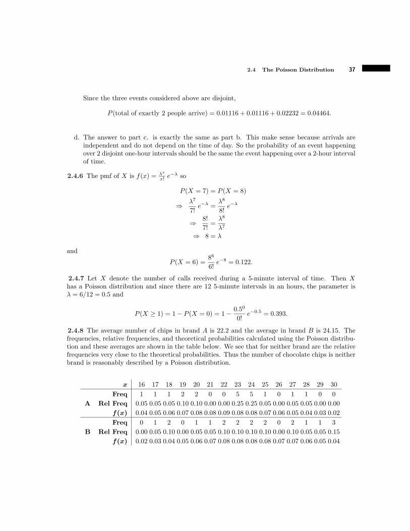
Since the three events considered above are disjoint,
P (total of exactly 2 people arrive) = 0.01116 + 0.01116 + 0.02232 = 0.04464.
d. The answer to part c. is exactly the same as part b. This make sense because arrivals areindependent and do not depend on the time of day. So the probability of an event happeningover 2 disjoint one-hour intervals should be the same the event happening over a 2-hour intervalof time.
2.4.6 The pmf of X is f(x) = "x
x! e!" so
P (X = 7) = P (X = 8)
% "7
7!e!" =
"8
8!e!"
% 8!
7!=
"8
"7
% 8 = "
and
P (X = 6) =86
6!e!8 = 0.122.
2.4.7 Let X denote the number of calls received during a 5-minute interval of time. Then Xhas a Poisson distribution and since there are 12 5-minute intervals in an hours, the parameter is" = 6/12 = 0.5 and
P (X " 1) = 1# P (X = 0) = 1# 0.50
0!e!0.5 = 0.393.
2.4.8 The average number of chips in brand A is 22.2 and the average in brand B is 24.15. Thefrequencies, relative frequencies, and theoretical probabilities calculated using the Poisson distribu-tion and these averages are shown in the table below. We see that for neither brand are the relativefrequencies very close to the theoretical probabilities. Thus the number of chocolate chips is neitherbrand is reasonably described by a Poisson distribution.
x 16 17 18 19 20 21 22 23 24 25 26 27 28 29 30
Freq 1 1 1 2 2 0 0 5 5 1 0 1 1 0 0
A Rel Freq 0.05 0.05 0.05 0.10 0.10 0.00 0.00 0.25 0.25 0.05 0.00 0.05 0.05 0.00 0.00
f(x) 0.04 0.05 0.06 0.07 0.08 0.08 0.09 0.08 0.08 0.07 0.06 0.05 0.04 0.03 0.02
Freq 0 1 2 0 1 1 2 2 2 2 0 2 1 1 3
B Rel Freq 0.00 0.05 0.10 0.00 0.05 0.05 0.10 0.10 0.10 0.10 0.00 0.10 0.05 0.05 0.15
f(x) 0.02 0.03 0.04 0.05 0.06 0.07 0.08 0.08 0.08 0.08 0.07 0.07 0.06 0.05 0.04

38 CHAPTER 2 Discrete Random Variables
2.4.9 The total number of knots observed is 0(28)+1(56)+· · ·+7(1) = 399. Since there were a totalof 200 boards, the average number of knots on a board is " = 399/200 $ 2. The frequencies, relativefrequencies, and theoretical probabilities calculated using the Poisson distribution with " = 2 areshown in the table below. We see that the relative frequencies are generally close to the theoreticalprobabilities. This indicates that the number of knots on a board is reasonably described by aPoisson distribution.
x 0 1 2 3 4 5 6 7
Freq 28 56 51 35 19 7 3 1
Rel Freq 0.14 0.28 0.26 0.18 0.10 0.04 0.02 0.01
f(x) 0.135 0.271 0.271 0.180 0.090 0.036 0.012 0.003
2.4.10 Since there are 100 small squares and a total of 30 dots, the average number of dots ina square is " = 30/100 = 0.3. The frequencies, relative frequencies, and theoretical probabilitiescalculated using the Poisson distribution with " = 0.3 are shown in the table below. We see thatthe relative frequencies are generally close to the theoretical probabilities. This indicates that thenumber of dots in a randomly chosen small square is reasonably described by a Poisson distribution.
x 0 1 2 3
Freq 72 26 2 3
Rel Freq 0.72 0.26 0.02 0.03
f(x) 0.741 0.222 0.033 0.003
2.4.11 Let X denote the number of winners out of 2000 tickets. Then X is b(2000, 0.001) and ap-proximately Poisson with parameter " = 2000(0.001) = 2. Notice that the rule-of-thumb conditionsare met, so the Poisson distribution o!ers a reasonable approximation.
a. P (X = 1) $ 21
1! e!2 = 0.271
b. P (4 ! X ! 6) $ 24
4! e!2 + 25
5! e!2 + 26
6! e!2 = 0.138
c. P (X < 3) $ 20
0! e!2 + 21
1! e!2 + 22
2! e!2 = 0.677
2.4.12 Let X denote the number of students out of 200 that get the flu. Then assuming the 4% ratehas not changed, X is b(200, 0.04) and approximately Poisson with parameter " = 200(0.04) = 8.Notice that the rule-of-thumb conditions are met, so the Poisson distribution o!ers a reasonableapproximation. Thus
P (X ! 2) $ 80
0!e!8 +
81
1!e!8 +
82
2!e!8 = 0.0138.
Since this probability is small, it appears that the assumption of a 4% rate is incorrect. Thus itappears the vaccine program has been e!ective.

2.4 The Poisson Distribution 39
2.4.13 Let X denote the number of cars that arrive at the toll booth in a one-minute interval oftime. Then X is Poisson with parameter " = 4 so the probability that exactly 10 cars arrive in aone-minute interval of time is
P (X = 10) =410
10!e!4 = 0.00529.
Now let Y denote the number of one-minute intervals of time out of 1000 in which exactly 10 carsarrive. Then Y is b(1000, 0.00529) and approximately Poisson with parameter " = 1000(0.00529) =5.292. Notice that the rule-of-thumb conditions are met, so the Poisson distribution o!ers a reason-able approximation of probabilities of Y . Then the probability that exactly 10 cars arrive in 8 outof 1000 di!erent one-minute intervals of time is
P (Y = 8) $ 5.2928
8!e!5.292 = 0.0767.
2.4.14 The total area occupied by the cow paties is 20, 000(0.5) = 10, 000 ft2. Thus the probabilitythat a single step hits a patty is 10, 000/(1000 · 1000) = 0.01. Let X denote the number of stepsout of 400 that hit a patty. Then X is b(400, 0.01) and approximately Poisson with parameter" = 400(0.01) = 4. Notice that the rule-of-thumb conditions are met, so the Poisson distributiono!ers a reasonable approximation. Thus
P (X " 1) = 1# P (X = 0) $ 1# 40
0!e!4 = 0.982.
2.4.15 Let X have a Poisson distribution with parameter ".
a. Note that for x = 1, 2, . . .,
P (X = x)
P (X = x# 1)=
"x
x! e!"
"x!1
(x!1)! e!"
="x
x!· (x# 1)!
"x!1
="
x.
b. If P (X = x) " P (X = x# 1), then by part a.,
1 ! P (X = x)
P (X = x# 1)=
"
x% x ! ".
c. By part b., P (X = x) " P (X = x # 1) for all x ! ". By a similar argument, we can showthat P (X = x) ! P (X = x# 1) for all x > ". Let f(x) denote the pmf of X and -". denotethe greatest integer less than or equal to ". The above arguments show that
f(0) ! · · · f (-". # 1) ! f (-".) > f (-".+ 1) " · · ·
Thus f attains its maximum value at X = -"., and by definition, the mode of X is -"..

40 CHAPTER 2 Discrete Random Variables
2.4.16 Let X denote the number of calls received in a one-hour interval of time. Then X has aPoisson distribution with parameter " = 8.4.
a. By part c. of exercise 2.4.15, the mode of this distribution is -8.4. = 8. This is the most likelynumber of calls received in an hour.
b. By part a. of exercise 2.4.15,
P (X = 8)
P (X = 7)=
8
8= 1 % P (X = 8) = P (X = 7).
showing that receiving 8 calls in an hour is just as likely as receiving 7 calls.
2.5 Mean and Variance
2.5.1
a. µ = 0(0.1) + · · ·+ 4(0.1) = 2.3,
#2 = (0# 2.3)2(0.1) + · · ·+ (4# 2.3)2(0.1) = 1.21,
# =/1.21 = 1.1
b. µ = #2(1/16) + · · ·+ 15(1/16) = 6,
#2 = (#2# 6)2(1/16) + · · ·+ (15# 6)2(1/16) = 112/3 = 37.33,
# =/112/3 = 6.11
c. µ = 3(1) = 3,
#2 = (3# 3)2(1) = 0,
# =/0 = 0
d. The values of the pmf are f(0) = 1/4, f(1) = 1/2, and f(2) = 1/4 so that
µ = 1(1/2) + 2(1/4) = 1,
#2 = (0# 1)2(1/4) + (1# 1)2(1/2) + (2# 1)2(1/4) = 1/2,
# =/1/2 = 0.707
2.5.2
a. The pmf is shown in the table below.
x 0 1 2 3 4
y -1 2 5 8 11
f(y) 0.1 0.1 0.3 0.4 0.1
b. µ = #1(0.1) + · · ·+ 11(0.1) = 5.9c. We see that E(Y ) = 3E(X)# 1.

2.5 Mean and Variance 41
2.5.3 The volumes of the boxes are 3 ft3, 21 ft3, and 60 ft3, so the mean volume is 3(0.35) +21(0.45) + 60(0.2) = 22.5 ft3.
2.5.4 Note that X has a uniform distribution with range R = {1, . . . , 9}, so E(X) = (9+1)/2 = 5and V ar(X) = (92 # 1)/12 = 20/3.
2.5.5 To find the mean, we need to find the parameter ". Let X denote the number of yellowcandies in a bag and f(x) denote its pmf We are told that P (X = 0) = 0.0183. Thus
f(0) ="0
0!e!" = 0.0183 % " = # ln 0.0183 $ 4
Thus the mean number of yellow candies in a bag is 4.
2.5.6 Suppose X is b(5, 0.20).
a. The pmf is given in the table below.
x 0 1 2 3 4 5
f(x) 0.3277 0.4096 0.2048 0.0512 0.0064 0.0003
b. µ = 0(0.3277) + · · ·+ 5(0.0003) = 1, #2 = (0# 1)2(0.3277) + · · ·+ (5# 1)2(0.0003) = 0.8c. Note that µ = 5(0.2) = np and #2 = 5(0.2)(0.8) = np(1# p).
2.5.7 The probability of getting a heart on either selection is 1/4. The probability of getting0 hearts is (3/4)(3/4) = 9/16, the probability of getting 1 heart is 2(1/4)(3/4) = 3/8, and theprobability of getting 2 hearts is (1/4)(1/4) = 1/16. Let X denote the number of hearts selected.The pmf of X is given in the table below.
x 0 1 2
f(x) 9/16 3/8 1/16
Thus the mean and variance of the number of hearts selected are
µ = 0(9/16) + 1(3/8) + 2(1/16) = 1/2 and
#2 = (0# 1/2)2(9/16) + (1# 1/2)2(3/8) + (2# 1/2)2(1/16) = 3/8.
2.5.8 The pmf of X is given in the table below.
x 0 1
f(x) 1# p p
Then E(X) = 0(1# p) + 1(p) = p and V ar(X) = (0# p)2(1# p) + (1# p)2(p) = p (1# p).
42 CHAPTER 2 Discrete Random Variables
2.5.9 The probability that X takes values “close” to 5 is large, so it has a relatively small standarddeviation. The probability that Z takes values “far” from 5 is large, so it has a relatively largestandard deviation. Z can take values “close” to 5 and “far” from 5 with relatively equal probability,so its standard deviation is somewhere between that of X and Z.
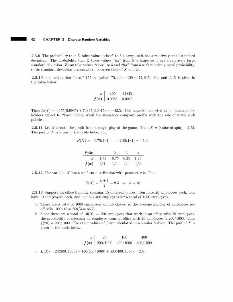
2.5.10 The male either “loses” 155 or “gains” 75, 000 # 155 = 74, 845. The pmf of X is given inthe table below.
x -155 74845
f(x) 0.9985 0.0015
Then E(X) = #155(0.9985) + 74845(0.0015) = #42.5. This negative expected value means policyholders expect to “lose” money while the insurance company profits with the sale of many suchpolicies.
2.5.11 Let X denote the profit from a single play of the game. Then X = (value of spin) # 2.75.The pmf of X is given in the table below and
E(X) = #1.75(1/4) + · · · 1.25(1/4) = #1/4.
Spin 1 2 3 4
x -1.75 -0.75 0.25 1.25
f(x) 1/4 1/4 1/4 1/4
2.5.12 The variable X has a uniform distribution with parameter k. Then
E(X) =k + 1
2= 9.5 % k = 18.
2.5.13 Suppose an o"ce building contains 15 di!erent o"ces. Ten have 20 employees each, fourhave 100 employees each, and one has 400 employees for a total of 1000 employees.
a. There are a total of 1000 employees and 15 o"ces, so the average number of employees pero"ce is 1000/15 = 200/3 = 66.7.
b. Since there are a total of 10(20) = 200 employees that work in an o"ce with 20 employees,the probability of selecting an employee from an o"ce with 20 employees is 200/1000. Thusf(20) = 200/1000. The other values of f are calculated in a similar fashion. The pmf of X isgiven in the table below.
x 20 100 400
f(x) 200/1000 400/1000 400/1000
c. E(X) = 20(200/1000) + 100(400/1000) + 400(400/1000) = 204.

2.5 Mean and Variance 43
2.5.14 The expected value of X is
E(X) =$%
x=1
x · 6
!2x2=
6
!2
$%
x=1
1
x.
But this is a p-series with p = 1 which diverges. Thus this expected value does not exist.
2.5.15 Using the identity$.
n=1nxn!1 = x
(1!x)2 for |x| < 1, the expected value of T is
E(T ) =$%
t=1
t · 1
10
#9
10
$t!1
=1
10
$%
t=1
t
#9
10
$t!1
=1
10· 9/10
(1# 9/10)2= 9.
2.5.16 Suppose it costs $n to play the game, and let X denote the “profit” from one play of thegame. Then X = (result from die)# n. The pmf of X is given in the table below.
Die 1 2 3
x 1# n 2# n 3# n
f(x) 3/6 2/6 1/6
ThenE(X) = (1# n)(3/6) + (2# n)(2/6) + (3# n)(1/6) = (10# 6n)/6.
For this to equal 0, we need n = 10/6 $ 1.67. Thus a “fair” price for the game is $1.67.
2.5.17
a. The game lasts n flips only if the first n # 1 flips are heads and the nth flip is tails. Theprobability of this is (1/2)n!1(1/2) = 1/2n. The pmf of X is given in the table below.
n 1 2 3 4
x 20 21 22 23
f(x) 1/2 1/22 1/23 1/24
b. You win less than $25 if the game lasts 4 flips or fewer. Thus
P (X ! 25) =1
2+ · · ·+ 1
24= 0.9375,
meaning we are very likely to lose money on this game so we would not want to play the game.
c. Note
E(X) = 201
2+ 21
1
22+ 22
1
23+ · · · =
$%
n=1
2n!1 1
2n=
$%
n=1
1
2.
But this series diverges to infinity, so E(X) does not exist. This means the game has aninfinite expected value.
44 CHAPTER 2 Discrete Random Variables
d. Since the expected value of the game is so large, we might be willing to play the game regardlessof the price. This does not agree with the answer in part b.
2.6 Functions of a Random Variable
2.6.1 E(X) = 0(1/4) + · · ·+ 3(1/4) = 13/8
E,X2-= 02(1/4) + · · ·+ 32(1/4) = 31/8
V ar(X) = 31/8# (13/8)2 = 79/64
E,X2 + 3X + 1
-= E
,X2-+ 3E(X) + 1 = 31/8 + 3(13/8) + 1 = 39/4
E,/
X + 5-=
/0 + 5(1/4) + · · ·+
/3 + 5(1/4) = 2.564
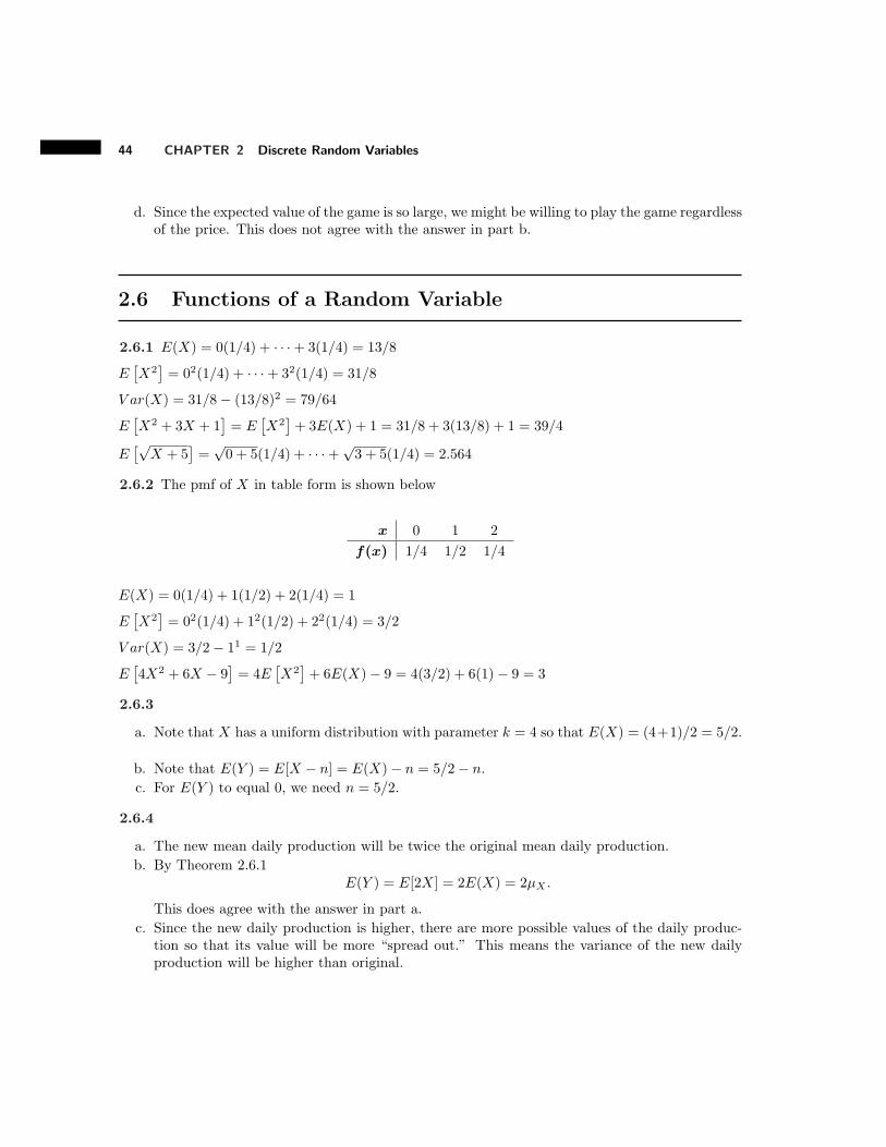
2.6.2 The pmf of X in table form is shown below
x 0 1 2
f(x) 1/4 1/2 1/4
E(X) = 0(1/4) + 1(1/2) + 2(1/4) = 1
E,X2-= 02(1/4) + 12(1/2) + 22(1/4) = 3/2
V ar(X) = 3/2# 11 = 1/2
E,4X2 + 6X # 9
-= 4E
,X2-+ 6E(X)# 9 = 4(3/2) + 6(1)# 9 = 3
2.6.3
a. Note that X has a uniform distribution with parameter k = 4 so that E(X) = (4+1)/2 = 5/2.
b. Note that E(Y ) = E[X # n] = E(X)# n = 5/2# n.c. For E(Y ) to equal 0, we need n = 5/2.
2.6.4
a. The new mean daily production will be twice the original mean daily production.b. By Theorem 2.6.1
E(Y ) = E[2X] = 2E(X) = 2µX .
This does agree with the answer in part a.c. Since the new daily production is higher, there are more possible values of the daily produc-
tion so that its value will be more “spread out.” This means the variance of the new dailyproduction will be higher than original.

2.6 Functions of a Random Variable 45
d. By Theorem 2.6.2V ar(Y ) = V ar[2X] = 22V ar(X) = 4#2
X .
This shows that the new variance is four times the old variance which agrees with the answerto part c.
2.6.5 Let µX = E(X). By Theorem 2.6.1, E[aX] = aE(X) = aµX , and by the definition ofvariance,
V ar[aX] = E0(aX # aµX)2
1= E
0a2 (X # µX)2
1
= a2E0(X # µX)2
1= a2V ar(X).
2.6.6 Since X takes on only one value, its pmf is f(x) = 1 for x = b. Thus E(X) = b and
V ar(X) = E,(X # b)2
-= (b# b)2(1) = 0.
2.6.7
a. The range of Y is R = {a, a+ 1, . . . , k + a# 1}. Since each value of X is equally likely, eachvalue of Y is also equally likely and the pmf of Y is f(y) = 1/k for all y , R.
b. Note that
E(Y ) = E [X + a# 1] = E(X) + a# 1 =k + 1
2+ a# 1
=k + 1 + 2a# 2
2=
a+ (k + a# 1)
2=
a+ b
2.
2.6.8 Note that by exercise 2.6.7, E(X) = (5 + 11)/2 = 8 so that
E(Y ) = E [120X # 200] = 120E(X)# 200 = 120(8)# 200 = 760.
2.6.9 Note that µX and #2X are constants. So by linearity properties of expected value,
E(Y ) = E
2X # µX
#X
3=
1
#X[E(X)# E (µX)] =
1
#X(µX # µX) = 0
and by the definition of #X ,
V ar(Y ) = E,(Y # 0)2
-= E
*#X # µX
#X
$2+=
1
#2X
E0(X # µX)2
1=
1
#2X
#2X = 1.
2.6.10
a. 5 = E[X # 5] = E(X)# 5 % E(X) = 10b. 30 = E
,(X # 5)2
-= E
,X2-# 10E(X) + 25 = E
,X2-# 75 % E
,X2-= 105
c. V ar(X) = E,X2-# [E(X)]2 = 105# 102 = 5
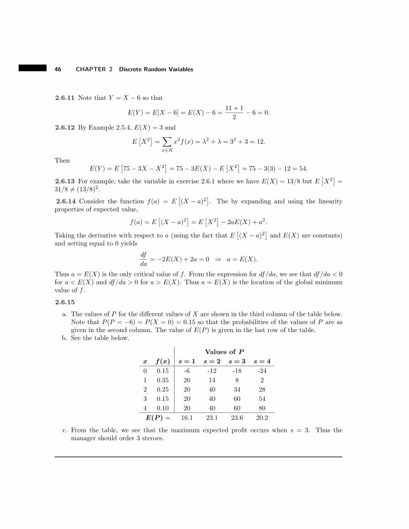
46 CHAPTER 2 Discrete Random Variables
2.6.11 Note that Y = X # 6 so that
E(Y ) = E[X # 6] = E(X)# 6 =11 + 1
2# 6 = 0.
2.6.12 By Example 2.5.4, E(X) = 3 and
E,X2-=%
x#R
x2f(x) = "2 + " = 32 + 3 = 12.
ThenE(Y ) = E
,75# 3X #X2
-= 75# 3E(X)# E
,X2-= 75# 3(3)# 12 = 54.
2.6.13 For example, take the variable in exercise 2.6.1 where we have E(X) = 13/8 but E,X2-=
31/8 += (13/8)2.
2.6.14 Consider the function f(a) = E,(X # a)2
-. The by expanding and using the linearity
properties of expected value,
f(a) = E,(X # a)2
-= E
,X2-# 2aE(X) + a2.
Taking the derivative with respect to a (using the fact that E,(X # a)2
-and E(X) are constants)
and setting equal to 0 yields
df
da= #2E(X) + 2a = 0 % a = E(X).
Thus a = E(X) is the only critical value of f . From the expression for df/da, we see that df/da < 0for a < E(X) and df/da > 0 for a > E(X). Thus a = E(X) is the location of the global minimumvalue of f .
2.6.15
a. The values of P for the di!erent values of X are shown in the third column of the table below.Note that P (P = #6) = P (X = 0) = 0.15 so that the probabilities of the values of P are asgiven in the second column. The value of E(P ) is given in the last row of the table.
b. See the table below.
Values of P
x f(x) s = 1 s = 2 s = 3 s = 4
0 0.15 -6 -12 -18 -24
1 0.35 20 14 8 2
2 0.25 20 40 34 28
3 0.15 20 40 60 54
4 0.10 20 40 60 80
E(P ) = 16.1 23.1 23.6 20.2
c. From the table, we see that the maximum expected profit occurs when s = 3. Thus themanager should order 3 steroes.

2.7 The Moment-Generating Function 47
2.7 The Moment-Generating Function
2.7.1 In each part below, the mgf for a discrete random variable X is given. For each, describe thepmf of X in table form, find M %(t) and M %%(t), and use these derivatives to calculate µ and #2.
a. The pmf is given in the table below.
x -1 3 4
f(x) 1/5 2/5 2/5
Now,
M %(t) = #1
5e!t +
6
5e3t +
8
5e4t and M %%(t) =
1
5e!t +
18
5e3t +
32
5e4t
so that
µ = M %(0) = 13/5 and #2 = M %%(0)# [M %(0)]2= 51/5# (13/5)2 = 86/25.
b. The pmf is given in the table below.
x 1 2 3 4 5
f(x) 0.2 0.2 0.2 0.2 0.2
Now,
M %(t) =5%
x=1
x(0.2)etx and M %%(t) =5%
x=1
x2(0.2)etx
so thatµ = M %(0) = 3 and #2 = M %%(0)# [M %(0)]
2= 11# (3)2 = 2.
2.7.2 Comparing M(t) = (0.25 + 0.75et)25
to the mgf in Example 2.7.3, we see that this is the mgfof a random variable that is b(25, 0.75).
2.7.3 By the definition of a mgf, M(0) = E,e0·X
-= E[1] = 1.
2.7.4 By the definition of the mgf,
M(t) = E,etX-= et(0)p0(1# p)1!0 + et(1)p1(1# p)1!1 = (1# p) + p et.
ThenM %(t) = p et and M %%(t) = p et
so that
E(X) = M %(0) = p and V ar(X) = M %%(0)# [M %(0)]2= p# p2 = p(1# p).

48 CHAPTER 2 Discrete Random Variables
2.7.5 By the rule for the derivative of the natural logarithm and the quotient rule,
R%(t) =M %(t)
M(t)and R%%(t) =
M(t)M %%(t)#M %(t)M %(t)
[M(t)]2
so that
R%(0) =M %(0)
M(0)=
µ
1= µ and R%%(0) =
M(0)M %%(0)#M %(0)M %(0)
[M(0)]2
=M %%(0)# [M %(0)]2
12= #2.
2.7.6 By the definition of E(X),
E(X) =$%
x=1
xa
x2= a
$%
x=1
1
x.
But this is a divergent p-series, so E(X) does not exist. If such a variable without an expected valuehad a mgf, then by the second part of Theorem 2.7.1, the expected value would exist and equalM %(0). But this is a contradiction. So a variable without an expected value cannot have a mgf
2.7.7 By definition of the mgf and linearity properties of expected value,
MY (t) = E,eY t-= E
0e(aX+b)t
1= E
0e(at)Xebt
1= ebtE
0e(at)X
1.
But E,e(at)X
-= MX(at) so that MY (t) = ebtMX(at) as desired.
2.7.8 By exercise 2.7.7, the mgf of Y = 2X + 4 is
MY (t) = e4tMX(2t) = e4t!0.5 + 0.3e2t + 0.2e6t
"= 0.5e4t + 0.3e6t + 0.2e10t.
2.7.9 By exercise 2.7.7, the mgf of Y = aX + b is MY (t) = ebtMX(at) so that
M %Y (t) = b ebtMX(at) + a ebtM %
X(at),
M %%Y (t) = b2 ebtMX(at) + 2ab ebtM %
X(at) + a2 ebtM %%X(at),
E(Y ) = M %Y (0) = b e0MX(0) + a e0M %
X(0) = b+ aE(X), and
V ar(Y ) = M %%Y (0)# [M %
Y (0)]2= b2 e0MX(0) + 2ab e0M %
X(0) + a2 e0M %%X(0)# [b+ aE(X)]2
= b2 + 2abE(X) + a2M %%X(0)# b2 # 2abE(X)# a2E(X)
= a2 [M %%X(0)# E(X)]
= a2V ar(X).
2.7.10 Let MX(t) = [ q + p et]ndenote the mgf of X. By exercise 2.7.7, the mgf of F = n #X is
MF (t) = entMX(#t) so that
MF (t) = entMX(#t) = ent,q + p e!t
-n=,et!q + p e!t
"-n=,p+ q et
-n.
This is the mgf of a random variable that is b(n, q).

2.7 The Moment-Generating Function 49
2.7.11
a. X is b(50, 0.0956) and E(X) = 50(0.0956) = 4.78.b. Note that T = 50 + 10X so that E(T ) = 50 + 10E(X) = 97.8.c. By combining samples, the lab expects to run about 100 tests. If they tested each individual
sample, they would have to run exactly 500 tests. So they are eliminating about 400 tests bycombining samples.
d. In general, E(T ) = 50 + 10E(X). For E(T ) to be less than 500, we need E(X) < 45. Nowlet p1 denote the probability that a combined sample tests positive. Then E(X) = 50p1. ForE(X) to be less than 45, we need p1 < 45/50 = 0.9. Generalizing the results of Exercise1.7.10, the probability that a combined sample tests positive is p1 = 1 # (1 # p)10. Thus weneed
1# (1# p)10 < 0.9 % p < 0.206.
Thus the method of testing combined samples saves work for p < 0.206.
2.7.12 By the definition of the mgf,
M(t) =,eXt-=
$%
x=1
extqx!1p =$%
x=1
etp!q et"x!1
.
Now, this is a geometric series which converges if |etq| < 1 % t < ln(1/q) so that
M(t) =p et
1# qetfor t < ln
#1
q
$.
Then, using the quotient rule and after algebraic simplification,
M %(t) =p et
(1# qet)2and M %%(t) =
p et (1 + qet)
(1# qet)3.
Then using the fact that 1# q = p, we get
E(X) = M %(0) =p e0
(1# qe0)2=
p
(1# q)2=
1
p, and
V ar(Y ) = M %%(0)# [M %(0)]2=
p e0!1 + qe0
"
(1# qe0)3##1
p
$2
=p (1 + q)
p3# 1
p2=
q
p2.
2.7.13 Note that
M %(t) = r
#p et
1# qet
$r!14(1# qet) p et # p et (#q et)
(1# qet)2
5
= r
#p et
1# qet
$r!14
p et
(1# qet)2
5
= r
#p et
1# qet
$r #1
1# qet
$.

50 CHAPTER 2 Discrete Random Variables
Then using the fact that 1# q = p, we get
E(X) = M %(0) = r
#p
1# q
$r # 1
1# q
$=
r
p.
2.7.14 The pmf of X is f(x) = "x
x! e!". Then by the definition of the mgf and the Taylor series
e"et
=$.x=0
("et)x
x! ,
M(t) = E,eXt-=
$%
x=0
ext"x
x!e!" = e!"
$%
x=0
("et)x
x!= e!"e"e
t
= e"(et!1).
2.7.15 Note that
M %(t) = e"(et!1) = e"(e
t!1) !"et"= "et+"(et!1) and
M %%(t) = "et+"(et!1) !1 + "et"
so that
E(X) = M %(0) = "e0+"(e0!1) = ", and
V ar(Y ) = M %%Y (0)# [M %
Y (0)]2= "e0+"(e0!1) !1 + "e0
"# "2 = "(1 + ")# "2 = ".
These derivatives were much easier to calculate than manipulating the infinite series in Example2.5.4.
2.7.16
a. Assuming the claim is true,X is b(100, 0.2) so that µ = 100(0.2) = 20 and # =/100(0.2)(0.8) =
4.
b. The “usual” minimum value is 20#2(4) = 12 and the “usual” maximum value is 20+2(4) = 28.
c. Since X = 10 is less than the “usual” minimum value, it is considered “unusual.” Thisindicates the claim may be incorrect.
2.7.17 The pmf of a random variable X with a Poisson distribution with parameter " is f(x) ="x
x! e!". Using the Taylor series e"t =
$.x=0
("t)x
x! , the probability-generating function is
P (t) =$%
x=0
"x
x!e!" tx = e!"
$%
x=0
("t)x
x!= e!"e"t = e"(t!1).
Note that this Taylor series converges for all t, so P (t) is defined for all t. Then
P %(t) = " e"(t!1) % E(X) = P %(1) = " e"(1!1) = ".

2.7 The Moment-Generating Function 51
2.7.18 The pmf of a random variable X that is b(n, p) is f(x) =!nx
"pxqn!x for x = 0, 1, . . . , n.
Using the binomial theorem (a+ b)n =n.
x=0
!nx
"an!xbx, the probability-generating function is
P (t) =n%
x=0
#n
x
$pxqn!xtx =
n%
x=0
#n
x
$(p t)xqn!x = (q + p t)n.
Note that this series is finite, so it converges for all t. Then using the fact that q + p = 1,
P %(t) = n(q + p t)n!1p % E(X) = P %(1) = n(q + p)n!1p = np.
2.7.19 The pmf of a random variable X with a geometric distribution is f(x) = qx!1p for x =1, 2, . . . where 0 ! p ! 1 and q = 1# p. Then
P (t) =$%
x=1
qx!1p tx =p
q
$%
x=1
(q t)(q t)x!1.
But this is a geometric series which converges if |q t| < 1 % |t| < 1/q. For |t| < 1/q,
P (t) =p
q
#q t
1# t
$=
p t
1# q t.
Then using the quotient rule,
P %(t) =p
(1# q t)2% E(X) = P %(1) =
p
(1# q)2=
1
p.

52 CHAPTER 2 Discrete Random Variables

Chapter 3
Continuous Random Variables
3.1 Introduction
3.2 Definitions
3.2.1
a. Note that (1# x)4 " 0 for all x, so f(x) " 0 for all x in its domain. Also,
6 $
!$f(x) dx =
6 1
05(1# x)4dx = #(1# x)5
7710= 0 + 1 = 1.
Thus the first two requirements for a pdf are met.b. The graph of the pdf is shown in the left half of Figure 3.1.c. The cdf is F (x) =
8 x!$ f(t) dt =
8 x0 5(1# t)4dt = #(1 # t)5 + 1 for 0 < x ! 1. The graph of
the cdf is shown in the right half of Figure 3.1.
d. P (0 < X ! 0.5) =8 0.50 5(1# x)4dx = 0.96875, P (X ! 0) = 0, P (X > 0.25) =
8 10.25 5(1# x)4dx $
0.2373
3.2.2
a. Note that all values of f(x) are non-negative, so f(x) " 0 for all x in its domain. Also,6 $
!$f(x) dx = 0.25(0.5) + 0.15(2) + 0.35(1) + 0.25(0.9) = 1.
Thus the first two requirements for a pdf are met.
53

54 CHAPTER 3 Continuous Random Variables
0
1
2
3
4
5
6
0 0.2 0.4 0.6 0.8 1
f(x)
x
Graph of p.d.f.
0
0.2
0.4
0.6
0.8
1
1.2
0 0.2 0.4 0.6 0.8 1
F(x)
x
Graph of c.d.f.
Figure 3.1
0
0.5
1
1.5
2
2.5
0 0.2 0.4 0.6 0.8 1
f(x)
x
Graph of p.d.f.
0
0.2
0.4
0.6
0.8
1
1.2
0 0.2 0.4 0.6 0.8 1
F(x)
x
Graph of c.d.f.
Figure 3.2
b. The graph of the pdf is shown in the left half of Figure 3.2.
c. From the graph of the pdf, we see that for 0 < x ! 0.25, F (x) = 0.5x. For 0.25 < x ! 0.4,F (x) = 0.5(0.25)+2(x# 0.25) = #0.375+2x. The calculations for other intervals are similar.The cdf as a piecewise function is shown below. The graph of the cdf is shown in the righthalf of Figure 3.2.
F (x) =
9::::::::;
::::::::<
0 x ! 0
0.5x 0 < x ! 0.25
#0.375 + 2x 0.25 < x ! 0.4
0.025 + x 0.4 < x ! 0.75
0.1 + 0.9x 0.75 < x ! 1
1 x > 1
d. P (0 < X ! 0.5) = 0.5(0.25) + 2(0.15) + 1(0.1) = 0.525, P (X ! 0) = 0, P (X > 0.25) =1# 0.5(0.25) = 0.875
3.2.3
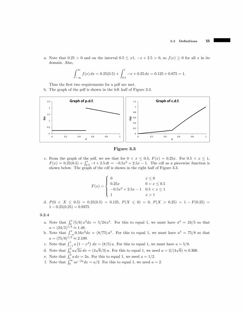
3.2 Definitions 55
a. Note that 0.25 > 0 and on the interval 0.5 ! x1, #x + 2.5 > 0, so f(x) " 0 for all x in itsdomain. Also,
6 $
!$f(x) dx = 0.25(0.5) +
6 1
0.5#x+ 0.25 dx = 0.125 + 0.875 = 1.
Thus the first two requirements for a pdf are met.b. The graph of the pdf is shown in the left half of Figure 3.3.
0
0.5
1
1.5
2
2.5
0 0.2 0.4 0.6 0.8 1
f(x)
x
Graph of p.d.f.
0
0.2
0.4
0.6
0.8
1
1.2
0 0.2 0.4 0.6 0.8 1
F(x)
x
Graph of c.d.f.
Figure 3.3
c. From the graph of the pdf, we see that for 0 < x ! 0.5, F (x) = 0.25x. For 0.5 < x ! 1,F (x) = 0.25(0.5) +
8 x0.5 #t+ 2.5 dt = #0.5x2 + 2.5x # 1. The cdf as a piecewise function is
shown below. The graph of the cdf is shown in the right half of Figure 3.3.
F (x) =
9:::;
:::<
0 x ! 0
0.25x 0 < x ! 0.5
#0.5x2 + 2.5x# 1 0.5 < x ! 1
1 x > 1
d. P (0 < X ! 0.5) = 0.25(0.5) = 0.125, P (X ! 0) = 0, P (X > 0.25) = 1 # F (0.25) =1# 0.25(0.25) = 0.9375
3.2.4
a. Note that8 a0 (5/6)x3dx = 5/24 a4. For this to equal 1, we must have a4 = 24/5 so that
a = (24/5)1/4 $ 1.48.b. Note that
8 a!a 0.16x
2dx = (8/75) a3. For this to equal 1, we must have a3 = 75/8 so that
a = (75/8)1/3 $ 2.109.
c. Note that8 1!1 a
!1# x4
"dx = (8/5) a. For this to equal 1, we must have a = 5/8.
d. Note that8 20 a
/3x dx = (4
/6/3) a. For this to equal 1, we need a = 3/(4
/6) $ 0.306.
e. Note that8 31 a dx = 2a. For this to equal 1, we need a = 1/2.
f. Note that8$0 ae!2xdx = a/2. For this to equal 1, we need a = 2.
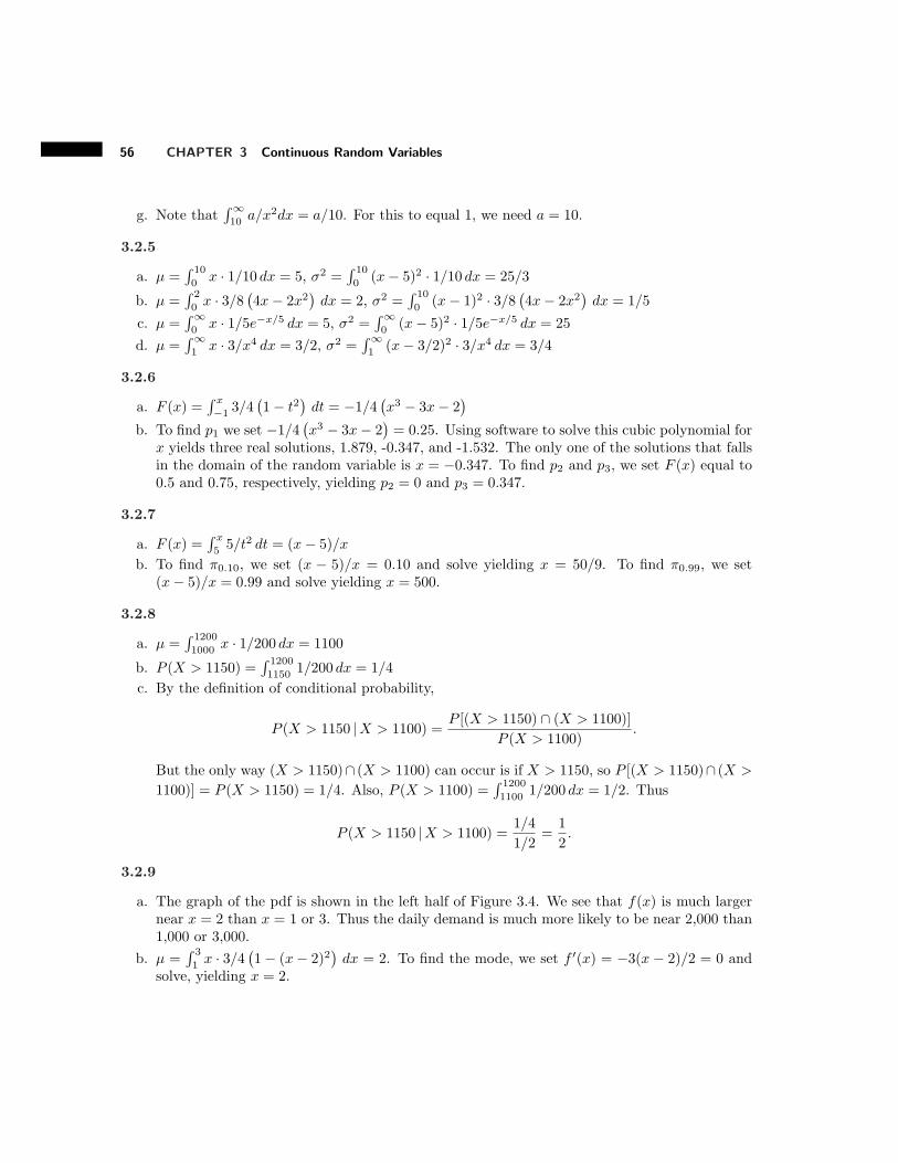
56 CHAPTER 3 Continuous Random Variables
g. Note that8$10 a/x2dx = a/10. For this to equal 1, we need a = 10.
3.2.5
a. µ =8 100 x · 1/10 dx = 5, #2 =
8 100 (x# 5)2 · 1/10 dx = 25/3
b. µ =8 20 x · 3/8
!4x# 2x2
"dx = 2, #2 =
8 100 (x# 1)2 · 3/8
!4x# 2x2
"dx = 1/5
c. µ =8$0 x · 1/5e!x/5 dx = 5, #2 =
8$0 (x# 5)2 · 1/5e!x/5 dx = 25
d. µ =8$1 x · 3/x4 dx = 3/2, #2 =
8$1 (x# 3/2)2 · 3/x4 dx = 3/4
3.2.6
a. F (x) =8 x!1 3/4
!1# t2
"dt = #1/4
!x3 # 3x# 2
"
b. To find p1 we set #1/4!x3 # 3x# 2
"= 0.25. Using software to solve this cubic polynomial for
x yields three real solutions, 1.879, -0.347, and -1.532. The only one of the solutions that fallsin the domain of the random variable is x = #0.347. To find p2 and p3, we set F (x) equal to0.5 and 0.75, respectively, yielding p2 = 0 and p3 = 0.347.
3.2.7
a. F (x) =8 x5 5/t2 dt = (x# 5)/x
b. To find !0.10, we set (x # 5)/x = 0.10 and solve yielding x = 50/9. To find !0.99, we set(x# 5)/x = 0.99 and solve yielding x = 500.
3.2.8
a. µ =8 12001000 x · 1/200 dx = 1100
b. P (X > 1150) =8 12001150 1/200 dx = 1/4
c. By the definition of conditional probability,
P (X > 1150 |X > 1100) =P [(X > 1150) ' (X > 1100)]
P (X > 1100).
But the only way (X > 1150)' (X > 1100) can occur is if X > 1150, so P [(X > 1150)' (X >
1100)] = P (X > 1150) = 1/4. Also, P (X > 1100) =8 12001100 1/200 dx = 1/2. Thus
P (X > 1150 |X > 1100) =1/4
1/2=
1
2.
3.2.9
a. The graph of the pdf is shown in the left half of Figure 3.4. We see that f(x) is much largernear x = 2 than x = 1 or 3. Thus the daily demand is much more likely to be near 2,000 than1,000 or 3,000.
b. µ =8 31 x · 3/4
!1# (x# 2)2
"dx = 2. To find the mode, we set f %(x) = #3(x # 2)/2 = 0 and
solve, yielding x = 2.
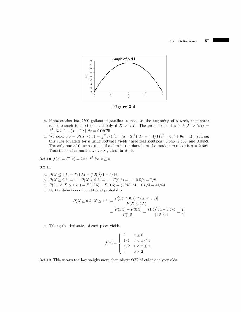
3.2 Definitions 57
0
0.1
0.2
0.3
0.4
0.5
0.6
0.7
0.8
1 1.5 2 2.5 3
f(x)
x
Graph of p.d.f.
Figure 3.4
c. If the station has 2700 gallons of gasoline in stock at the beginning of a week, then thereis not enough to meet demand only if X > 2.7. The probably of this is P (X > 2.7) =8 32.7 3/4
!1# (x# 2)2
"dx = 0.06075.
d. We need 0.9 = P (X < a) =8 a1 3/4
!1# (x# 2)2
"dx = #1/4
!a3 # 6a2 + 9a# 4
". Solving
this cubi equation for a using software yields three real solutions: 3.346, 2.608, and 0.0458.The only one of these solutions that lies in the domain of the random variable is a = 2.608.Thus the station must have 2608 gallons in stock.
3.2.10 f(x) = F %(x) = 2x e!x2
for x " 0
3.2.11
a. P (X ! 1.5) = F (1.5) = (1.5)2/4 = 9/16b. P (X " 0.5) = 1# P (X < 0.5) = 1# F (0.5) = 1# 0.5/4 = 7/8c. P (0.5 < X ! 1.75) = F (1.75)# F (0.5) = (1.75)2/4# 0.5/4 = 41/64d. By the definition of conditional probability,
P (X " 0.5 |X ! 1.5) =P [(X " 0.5) ' (X ! 1.5)]
P (X ! 1.5)
=F (1.5)# F (0.5)
F (1.5)=
(1.5)2/4# 0.5/4
(1.5)2/4=
7
9.
e. Taking the derivative of each piece yields
f(x) =
9:::;
:::<
0 x ! 0
1/4 0 < x ! 1
x/2 1 < x ! 2
0 x > 2
3.2.12 This means the boy weighs more than about 90% of other one-year olds.

58 CHAPTER 3 Continuous Random Variables
3.2.13 For t += 0, M(t) =8 41 ext · 1/3 dx =
!e4t # et
"/(3t). For t = 0, M(0) =
8 41 ex0 · 1/3 dx = 1.
3.2.14 Note that M(t) =8$0 exte!x dx =
8$0 e(t!1)x dx. But the exponent is non-negative for
t " 1 which would mean that the integral does not converge. Thus the integral converges, and M(t)exists only for t < 1. For t < 1, this integral converges to 1/(1# t).
3.2.15 By defintion and properties of expected value, M(0) = E,e0x-= E(1) = 1.
3.2.16 By defintion, #2 =8$!$ (x# µ)2f(x) dx. But (x # µ)2 " 0 and by definition of the pdf,
f(x) " 0 for all x. Thus the integrand is non-negative for all x. By properties of the definiteintegral, the value of this integral, assuming it exists, will be non-negative.
3.2.17 By defintion,
P=x0 #
$
2< X < x0 +
$
2
>=
6 x0+#/2
x0!#/2f(x) dx
But since f is continuous on [x0 # $/2, x0 + $/2], by the mean value theorem for integrals, thereexists an x1 , [x0 # $/2, x0 + $/2] such that the integral equals $ · f (x1). But $ is “small” so that[x0 # $/2, x0 + $/2] is “narrow.” Thus x1 is “close” to x0 and f (x1) $ f (x0). Therefore,
P=x0 #
$
2< X < x0 +
$
2
>= $ · f (x1) $ $ · f (x0) .
3.2.18
a. Tyson has a positive probability of parking any distance from the door. Since he looks for aspot close to the door, XT may have a relatively large probability of being small. But sincehe sometimes has to park far away, XT may have a relatively large probability of being large.Kylie only parks far away, so XK is small with probability 0. Based on these arguments,Possible graphs of the pdf’s are shown in Figure 3.5.
f(x)
x (Distance from front door)
Graph of p.d.f. of XT
f(x)
x (Distance from front door)
Graph of p.d.f. of XK
Figure 3.5
b. The mean of XK is probably larger than the mean of XT since Tyson sometimes parks closeto the door while Kylie never does. The variance of XT is probably larger than the varianceof XK since XT can take on a wider range of values thatn XK .

3.3 The Uniform and Exponential Distributions 59
c. Since Kylie always parks in roughly the same spot everyday, it takes her about the sameamount of time to walk from her car to the front door everyday so that the range of YK isnarrow. This is not the case for Tyson. Some days he may have a short distance to walk andsome days he has a long distance to walk. So the variance of YT is probably larger than thevariance of YK .
d. Since it takes Kylie roughly the same amount of time to reach the front door everyday, shewill have about the same amount of free-time before school everyday. Tyson will have a lot oftime on some days, and not as much on other days.
3.3 The Uniform and Exponential Distributions
3.3.1
a. This does not have a uniform distribution because the dart is more likely to lad “far” fromthe center than “near” the center.
b. Since the students are instructed to randomly cut the string, it is reasonable to assume thatX is uniform with a = 0 and b = 6.
c. The student is more likely to arrive “close” to the class start time than a long time before orafter the start time. So X is more likely to take values close to 0 than other values. Thus isit not reasonable to assume that X has a uniform distribution.
d. Since they agree to meet sometime between 6:00 and 6:15 PM with no “target” time, it isreasonable to assume that X is uniform with a = 0 and b = 15.
e. Since they agree to meet at 6:00 PM, it is more likely she will arrive “close” to 6:00 than along time before or after 6:00. So X is more likely to take values close to 0 than any othervalues. Thus is it not reasonable to assume that X has a uniform distribution.
3.3.2 We know from the text that E(X) = (a+ b)/2 so that
V ar(X) =
6 b
a
#x# a+ b
2
$2 1
b# adx
=1
3(b# a)
#x# a+ b
2
$377777
x=b
x=a
=1
3(b# a)
*##a+ b
2
$3
##a# b
2
$3+
=1
3(b# a)
*#b# a
2
$3
+
#b# a
2
$3+
=1
3(b# a)
#2(b# a)3
23
$
=(b# a)2
12.

60 CHAPTER 3 Continuous Random Variables
Also, for t += 0,
M(t) =
6 b
aetx
1
b# adx =
1
t(b# a)etx7777x=b
x=a
=etb # eta
t(b# a).
3.3.3
a. E(X) = (25 + 15)/2 = 20b. V ar(X) = (25# 15)2/12 = 25/3c. P (18 < X < 23) = (23# 18)/(25# 15) = 1/2d. P (12 < X < 18) = (18# 15)/(25# 15) = 3/10
3.3.4
a. P (4X + 2 < 4) = P (X < 1/2) = 1/2,b. P (3 < 4X + 2 < 5) = P (1/4 < X < 3/4) = 1/2,
3.3.5 By subtracting c and dividing by d# c, we get
P (c+ 0.5 < X · (d# c) + c < c+ 1.5) = P
#0.5
d# c< X <
1.5
d# c
$=
1
d# c
(note that d# c > 1.5 so that 1.5/(d# c) < 1). Using the same algebra, we get
2P (c < X · (d# c) + c < c+ 0.5) = 2P
#0 < X <
0.5
d# c
$= 2
#0.5
d# c
$=
1
d# c.
Thus these two probabilities are indeed equal.
3.3.6 Since #2 ! X ! 2, P (|X| > 1) = P [(#2 < X < #1) ( (1 < X < 2)] = P (#2 < X <#1) + P (1 < X < 2) = 1/4 + 1/4 = 1/2.
3.3.7
a. Note that P (X < d) = d!ab!a . Setting this equal to 0.75 and solving for d yields d = 0.75b+0.25a.
b. Note that P (c < X) = b!cb!a . Setting this equal to 0.90 and solving for c yields c = 0.9a+0.1b.
c. Note that since 0 < c < b!a2 , a+b
2 # c > a and a+b2 + c < b so that
P
#a+ b
2# c < X <
a+ b
2+ c
$=
2c
b# a.
Setting this equal to 0.6 and solving for c yields c = 0.3(b# a).d. Note that P (c < X < d) = d!c
b!a . Setting this equal to 0.3 yields d# c = 0.3(b# a). But thereare an infinite number of values of d and c in the interval (a, b) that solve this equation.
3.3.8 The pdf of X is f(x) = 1/4 for 15 < x < 19 and 0 otherwise. The engineer mistakely sub-tracted 16 and 14 and then multiplied by 1/4 obtaining 1/2. To correctly calculate the probability,we need to note that P (14 < X < 16) = P (14 < X < 15) = 1/4.

3.3 The Uniform and Exponential Distributions 61
3.3.9
a. Let X denote the time (in minutes) past 6:00 AM the passenger arrives. Then X is U(0, 40).Since the train arrives at 6:00, 6:20, and 6:40, the passenger will have to wait less than 5minutes if 15 < X ! 20 or 35 < X ! 40 so that
P (waiting longer than 5 min) = P [(15 < X ! 20) ( (35 < X ! 40)]
= P (15 < X ! 20) + P (35 < X ! 40)
= 5/40 + 5/40 = 1/4.
b. The passenger will have to wait more than 10 minutes if 0 < X < 10 or 20 < X < 30. Thishas probability of 10/40 + 10/40 = 1/2.
3.3.10 Let X denote the time (in minutes) past 9:00 AM the call arrives. Then X is U(0, 60) sothat P (20 < X < 45) = 5/60 = 5/12.
3.3.11 Let X denote the time (in hours) between the arrivals of the calls. Since the number ofcalls received in an hour is described by a Poisson distribution with parameter " = 4, X has anexponential distribution with " = 4 so that P (X > 20/60) = e!4(1/3) = 0.264.
3.3.12 Note that since E(X) = 0.5, the X has parameter " = 1/0.5 = 2. The dart will hit thebullseye if X is less than the radius of the bullseye so that P (hitting the bullseye) = P (X < 5/16) =1# e!2(5/16) = 0.465.
3.3.13
a. By the definition of conditional probability,
P (X > 2 + 1 |X > 1) =P [(X > 2 + 1) ' (X > 1)]
P (X > 1)=
P (X > 3)
P (X > 1)
=e!2(3)
e!2(2)= e!2(2) = P (X > 2).
b. By the definition of conditional probability,
P (X > a+ b |X > b) =P [(X > a+ b) ' (X > b)]
P (X > b)=
P (X > a+ b)
P (X > b)
=e!"(a+b)
e!"(b)= e!"(a)) = P (X > a).
3.3.14
a. Since X is exponentially distributed with parameter " = 0.001, P (X > 200) = e!0.001(200) =0.819.

62 CHAPTER 3 Continuous Random Variables
b. Using the results from exercise 3.3.13, we get
P (X > 1100 |X > 900) = P (X > 200 + 900 |X > 900) = P (X > 200) = 0.819.
c. The results from part b. mean that the probability the bulb lasts at least another 200 hoursafter it has lasted 900 hours (call this probability p1) is equal to the probably that a brandnew bulb lasts at least 200 hours (call this probability p2). This does not seem reasonable. Itis more reasonable to believe that p1 should be less than p2. Thus the assumption that X hasan exponential distribution does not seem reasonable.
3.3.15
a. To find !0.25, we set F (x) = 1# e!1/4x = 0.25 and solve for x, yielding !0.25 = 1.15.
b. To find !0.95, we set F (x) = 1# e!0.1x = 0.95 and solve for x, yielding !0.95 = 29.96.
c. To find !p, we set F (x) = 1# e!"x = p and solve for x, yielding !p = ln(1# p)/(#").
3.3.16 Note that the cdf of X is F (x) = (x# a)/(b# a) for a < x < b.
a. To find !0.12, we set F (x) = (x# 0)/(1# 0) = 0.12 and solve for x, yielding !0.12 = 0.12.
b. To find !0.99, we set F (x) = (x+8)/(15.5+ 8) = 0.99 and solve for x, yielding !0.99 = 15.265.
c. To find !p, we set F (x) = (x# a)/(b# a) = p and solve for x, yielding !p = p(b# a) + a.
3.3.17 To find the median of an exponential distribution, we set F (x) = 1# e!"x = 0.5 and solvefor x, yielding m = ln(0.5)/(#").
To find the median of a uniform distribution, we set F (x) = (x# a)/(b# a) = 0.5 and solve for x,yielding m = 0.5(b# a) + a.
3.3.18 The calculations are summarized in the table below and the relative frequency histogram isshown in Figure 3.6. We see that the relative frequencies are close to the theoretical probabilitiesand the histogram is “flat.” This means that it is reasonable to assume that X is U(5, 20).
Interval (5, 8] (8, 11] (11, 14] (14, 17] (17, 20]
Freq 6 7 6 7 4
Rel Freq 0.20 0.23 0.20 0.23 0.13
Theo Prob 0.2 0.2 0.2 0.2 0.2
3.3.19 The mean of the data is x = 5.15 so if X has an exponential distribution, then its parameter" $ 1/5.15 = 0.194. The calculations are summarized in the table below and the relative frequencyhistogram is shown in Figure 3.7. We see that the relative frequencies are not close to the theoreticalprobabilities and the histogram does not have the shape of an exponential density curve. This meansthat it is not reasonable to assume that X has an exponential distribution.

3.3 The Uniform and Exponential Distributions 63
0
0.05
0.1
0.15
0.2
0.25
6.5 9.5 12.5 15.5 18.5R
el F
req
Gallons
Figure 3.6
Interval (0, 2] (2, 4] (4, 6] (6, 8] (8, 10] (10, 12]
Freq 1 8 13 5 2 1
Rel Freq 0.03 0.27 0.43 0.17 0.07 0.03
Theo Prob 0.32 0.22 0.15 0.10 0.07 0.05
00.050.10.150.20.250.30.350.40.450.5
1 3 5 7 9 11
Rel
Fre
q
Time
Figure 3.7
3.3.20
a. To find To find the skewness of the exponential distribution, first note that µ = # = 1/".Next note that
M %%%(t) =d
dtM %%(t) =
d
dt
#2"
("# t)3
$=
6"
("# t)4
so that E,X3-= M %%%(0) = 6/"3 and
%1 =6/"3 # 3(1/")(1/")2 # (1/")3
(1/")3=
2/"3
(1/")3= 2.

64 CHAPTER 3 Continuous Random Variables
b. To find the skewness of the uniform distribution, we have µ = (a+ b)/2 and #2 = (b# a)2/12so that
%1 = E
?
@4X # (a+ b)/2/
(b# a)2/12
53A
B =
#12
(b# a)2
$3/2
E
*#X # a+ b
2
$3+.
Now by definition of the expected value of a function of a random variable and elementarycalculus,
E
*#X # a+ b
2
$3+=
6 b
a
#X # a+ b
2
$3 1
b# adx = 0.
Thus the skewness is %1 = 0.
3.3.21 We have µ = # = 1/". By the results of the calculations immediately following Example3.3.5, E
,X2-= M %%(0) = 2/"2. By the solution to exercise 3.3.20, E
,X3-= M %%%(0) = 6/"3. Also,
using the results of this solution,
M %%%%(t) =d
dtM %%%(t) =
d
dt
#6"
("# t)4
$=
24"
("# t)5
so that E,X4-= M %%%%(0) = 24/"4. Thus
%2 =24/"4 # 4(1/")
!6/"3
"+ 2(1/")2
!2/"2
"+ 5(1/")4
(1/")4# 3 =
9/"4
(1/")4# 3 = 6.
3.4 The Normal Distribution
Note: All probabilities were found using Table C.1.
3.4.1
a. P (Z > 1.78) = 1# 0.9625 = 0.0375b. P (#1.54 < Z ! 0.98) = 0.8365# 0.0618 = 0.7747c. P (|Z| > 2.5) = P [(Z < #2.5) ( (Z > 2.5)] = 2(0.0062) = 0.0124d. P (Z2+1 < 2.6) = P (Z2 < 1.6) = P (|Z| <
/1.6) = P (#1.26 < Z < 1.26) = 0.8962#0.1038 =
0.7924
3.4.2
a. P (X > 13.4) = P [Z > (13.4# 12)/1.4] = P (Z > 1) = 1# 0.8413 = 0.1587b. P (10.5 < X ! 14.5) = P [(10.5 # 12)/1.4 < Z ! (14.5 # 12)/1.4] = P (#1.07 < Z ! 1.79) =
0.9633# 0.1423 = 0.8210c. P (|X # 12| > 0.9) = P [(X # 12 < #0.9) ( (X # 12 > 0.9)] = P [(X < 11.1) ( (X > 12.9)] =
P ((Z < #0.64) ( (Z > 0.64)] = 0.2611 + (1# 0.7389) = 0.5222

3.4 The Normal Distribution 65
d. P (X2 + 10 < 110) = P (|X| < 10) = P (#10 < X < 10) = P (#15.71 < Z < #1.43) =0.0764# 0.0001 = 0.0763
e. P (X > 14 |X > 13.4) = P [(X>14)&(X>13.4)]P (X>13.4) = P (X>14)
P (X>13.4) =P (Z>1.43)P (Z>1) = 1!0.9236
1!0.8413 = 0.4814
3.4.3
a. Note that P (150 < X < 190) = P (#0.76 < Z < 0.62) = 0.7324 # 0.2236 = 0.5088. Thusabout 50.88% of people weigh between 150 and 190 pounds.
b. From Table C.1, we see that P (Z < 1.645) $ 0.95. To find !0.95, we then solve 1.645 =(x# 172)/29 for x yielding !0.45 = 168.4.
c. From Table C.1, we see that P (Z < #0.125) $ 0.45. To find !0.45, we then solve #0.125 =(x# 172)/29 for x yielding !0.95 = 219.7.
3.4.4 Note that if x = µ+a# where a is any number, then the z-score of x is z = (µ+a##µ)/# = a.We use this formula to calculate the following probabilities:
a. P (µ# # < X ! µ+ #) = P (#1 < Z ! 1) = 0.8413# 0.1587 = 0.6826 $ 0.68b. P (µ# 2# < X ! µ+ 2#) = P (#2 < Z ! 2) = 0.9772# 0.0228 = 0.9544 $ 0.95c. P (µ# 3# < X ! µ+ 3#) = P (#3 < Z ! 3) = 0.9987# 0.0013 = 0.9974 $ 0.997
3.4.5
a. Packages between 31.4 and 33.6 ounces are within one standard deviation of the mean, soabout 68% of packages fall within this range.
b. Packages between 30.3 and 34.7 ounces are within two standard deviations of the mean, soabout 95% of packages fall within this range.
c. Packages between 29.2 and 35.8 ounces are within three standard deviations of the mean, soabout 99.7% of packages fall within this range.
3.4.6 The emperical rule says that P (µ## < X ! µ+#) $ 0.68. This means that P (X ! µ+#) $0.68 + 0.5(1 # 0.68) = 0.84. But by definition, !0.84 is a number such that P (X ! !0.84) = 0.84.This shows that !0.84 $ µ+ #. By similar arguments, !0.975 $ µ+ 2# and !0.999 $ µ+ 3#.
3.4.7 In general, to find a number c > 0 such that P (#c < Z ! c) = p, we look through TableC.1 for a number c such that P (#c < Z) = 0.5(1 # p). This yields the solutions: a. c = 1.645, b.c = 1.96, c. c = 2.575.
3.4.8 Let X denote the actual amount spent on gasoline. Then X is N!185, 102
"so that
P (X > 200) = P (Z > (200# 185)/10) = P (Z > 1.5) = 1# 0.9332 = 0.0668.
Since this probability is small, the budgeted amount seems reasonable.
3.4.9 Let X denote the actual diameter of a randomly selected bolt. Then X is N!3.002, 0.0022
".
A bolt is accepted if 2.995 < X < 3.005 so that
P (A bolt is scrapped) = 1# P (A bolt is accepted)
= 1# P (2.995 < X < 3.005) = 1# P (#3.5 < Z < 1.5)
= 1# (0.9332# 0.0001) = 0.0669.
This means tha about 6.69% of all bolts will be scrapped.

66 CHAPTER 3 Continuous Random Variables
3.4.10 We need to find µ such that P (X < 12) = 0.015. Examining Table C.1, we see thatthe corresponding z-score is -2.17. Thus we need #2.17 = (12 # µ)/0.1. Solving this for µ yieldsµ = 12.217.
3.4.11 Note that
P (125 < Y ! 175) = P!125 < eX ! 175
"
= P (! 125 < X ! ln 175)
= P (#0.17 < Z < 0.16) = 0.5636# 0.4325 = 0.1311
3.4.12 The calculations are summarized in the table below and the relative frequency histogram isshown in Figure 3.8. We see that the relative frequencies are close to the theoretical probabilitiesand the histogram resembles the shape of a bell-curve. This means that it is reasonable to assumethat the height has a normal distribution.
Interval (#0, 61] (61, 63] (63, 65] (65, 67] (67, 0)
Freq 3 6 11 8 2
Rel Freq 0.100 0.200 0.367 0.267 0.067
Theo Prob 0.149 0.256 0.307 0.201 0.087
00.050.10.150.20.250.30.350.4
60 62 64 66 68
Rel
Fre
q
Height
Figure 3.8
3.4.13 The mean of a normally distributed random variable equals the horizontal location of thepeak of the bell-curve. Based on this, we see that Y has the largest mean and X has the smallest.The variance is determined by the shape of the bell-curve. The shorter and “fatter” the curve is, thehigher the variance. Based on this, we see that Z has the largest variance and X has the smallest.
3.4.14 First note that from the text, we have
E!X2"= M %%(0) = #2 + µ2 = 11 + 62 = 37.
Now, the length of one piece of spaghetti is X and the length of the other piece is 10 #X so thatthe area of the rectangle is A = X(10#X) = 10X #X2. Then by properties of expected value,
E(A) = E,10X #X2
-= 10E(X)# E
!X2"= 10(6)# 37 = 23.
3.4 The Normal Distribution 67
3.4.15
a. Note that f(#z) = 1'2!
e!(!z)2/2 = 1'2!
e!z2/2 = f(z).
b. Note that
f(µ# h) =1
#/2!
e!(µ!h!µ)2/(2$2) =1
#/2!
e!(!h)2/(2$2) =1
#/2!
e!h2/(2$2) and
f(µ+ h) =1
#/2!
e!(µ+h!µ)2/(2$2) =1
#/2!
e!h2/(2$2).
Thus f(µ# h) = f(µ+ h) as desired.
c. By definition, the median of a random variable X that is N!µ, #2
"is a number m such
that P (X < m) = 0.5. From Table C.1, we see that the corresponding z-score is 0 so that0 = (m#µ)/#. Solving this for m, we get m = µ. Thus the median of the normal distributionis µ.
d. The mode is a value of x for which f(x) is maximized. We have
d
dxf(x) =
1
#/2!
e!(x!µ)2/(2$2)##2(x# µ)
2#2
$.
Setting this equal to 0 and solving for x yields x = µ. Since the sign of f %(x) is determinedby the sign of the fraction on the right-end, we see that f %(x) > 0 for x < µ and f %(x) < 0 forx > µ. Thus by the first-derivative test, µ is the location of a local maximum. This provesthat µ is the mode of the normal distribution.
e. As shown in part d., the maximum value of f(x) occurs at x = µ. But f(µ) = 1/!#/2!".
This is the maximum value of f(x).
3.4.16 The mgf of X is MX(t) = expCµt+ $2
2 t2D. By exercise 2.7.7, the mgf of Z = X!µ
$ =1$ X + !µ
$ is
MZ(t) = exp
E#µ
#t
FMX
#1
#t
$
= exp
E#µ
#t
Fexp
Gµ
#1
#t
$+
#2
2
#1
#t
$2H
= exp
G#µ
#t+ µ
#1
#t
$+
#2
2
#1
#t
$2H
= exp
Et2
2
F.
But this is the mgf of a random variable with a standard normal distribution. Thus Z has a standardnormal distribution which proves Theorem 3.4.1.
68 CHAPTER 3 Continuous Random Variables
3.4.17 Note that
df
dx=
1
#/2!
e!(x!µ)2/(2$2)##2(x# µ)
2#2
$and
d2f
dx2=
1
#/2!
e!(x!µ)2/(2$2)
*##2(x# µ)
2#2
$2
+
##2
2#2
$+
The sign of d2fdx2 is determined by the expression in the square brackets. Simplifying this we get
*##2(x# µ)
2#2
$2
+
##2
2#2
$+=
(x# µ)2 # #2
#4.
Setting this equal to 0 yields (x # µ)2 = #2 which has solutions x = µ ± #. A quick check of the
signs shows that d2fdx2 > 0 for x < µ # # and x > µ + # and that d2f
dx2 < 0 for µ # # < x < µ + #.
Thus d2fdx2 changes signs at x = µ± #.
3.4.18 First note that
M %%(t) = et2/2!1 + t2
",
M %%%(t) = et2/2!t3 + 3t
", and
M %%%%(t) = et2/2!t4 + 6t2 + 3
"
so that E,X2-= M %%(0) = 1, E
,X3-= M %%%(0) = 0, and E
,X4-= M %%%%(0) = 3. Thus the skewness
is
%1 =E,X3-# 3µ#2 # µ3
#3=
0# 3(0)(1)# 03
13= 0
and the kurtosis is
%2 =E,X4-# 4µE
,X3-+ 2µ2E
,X2-+ 5µ4
#4# 3 =
3# 4(0)(0) + 2(0)2(1) + 5(0)4
14# 3 = 0.
3.4.19 Plugging z = 0.1236 into this formula yields P (Z ! 0.1236) $ 0.54917.
3.4.20 By basic algebra and properties of limits, we have
limz"$
P=Z > z +
a
z
>
P (Z > z)= lim
z"$
1# #=z +
a
z
>
1# #(z)
= limz"$
1
(z # a/z)/2!
e!(z!a/z)2/2
1
z/2!
e!z2/2
= limz"$
z
z # a/ze!a e!a2/(2z2)
= e!a.

3.5 Functions of Continuous Random Variables 69
3.5 Functions of Continuous Random Variables
3.5.1 First note that Y " (b# a) · 0 + a = a and Y ! (b# a) · 1 + a = b, so a ! Y ! b. Now,
F (y) = P (Y ! y) = P [(b# a)X + a ! y] = P
#X ! y # a
b# a
$
but 0 ! y # a
b# a! 1, so P
#X ! y # a
b# a
$=
y # a
b# a. Thus
f(y) =d
dyF (y) =
d
dy
#y # a
b# a
$=
1
b# a
which shows that Y is U(a, b).
3.5.2 First note that since 0 < X < 1, 0 < Y < 1. Then for 0 < y < 1,
F (y) = P (Y ! y) = P!X2 ! y
"= P (X ! /
y) =
6 'y
02x dx = y.
Thus f(y) = F %(y) = 1. Therefore, Y is U(0, 1).
3.5.3 First note that X > 0 and Y > 0. Then for y > 0,
F (y) = P (Y ! y) = P!X2 ! y
"= P (X ! /
y) =
6 'y
0
x
4e!x/2 dx
and
f(y) =dF
dy=
/y
4e!
'y/2
#1
2y!1/2
$=
1
8e!
'y/2.
3.5.4 First note that a < X < b and a2 ! Y ! b2. Then for a2 ! y ! b2
F (y) = P (Y ! y) = P!X2 ! y
"= P (X ! /
y) =
6 'y
0
1
b# adx
and
f(y) =dF
dy=
1
b# a
#1
2y!1/2
$=
1
2/y(b# a)
.
3.5.5 The area is A = X2 by exercise 3.5.4, the pdf of A is 12'a(3!2)
so that
P (5 < A < 6) =
6 6
5
1
2/ada =
/6#
/5 $ 0.213.

70 CHAPTER 3 Continuous Random Variables
3.5.6 First note that since 0 < X < 1, #1 < Y < 1. Then for #1 < y < 1,
F (y) = P (Y ! y) = P!(1# 2X)3 ! y
"= P
#X " 1# y1/3
2
$=
6 1
(1!y1/3)/23(1# 2x)2 dx
and
f(y) =dF
dy= #3
21# 2
#1# y1/3
2
$32·21
2
##1
3y!2/3
$3=
1
2.
Thus Y is U(#1, 1).
3.5.7 First note that since #4 ! X ! 5, 0 ! Y ! 25. Then
F (y) = P (Y ! y) = P!X2 ! y
"= P (|X| ! /
y) = P (#/y ! X ! /
y) .
Now, if 0 ! y ! 16, then #/y " #4 so that
P (#/y ! X ! /
y) =2/y
9.
If 16 < y ! 25, then #/y < #4 so that
P (#/y ! X ! /
y) = P (#4 ! X ! /y) =
/y + 4
9.
Thus we have
F (y) =
G2/y/9 0 ! y ! 16
(/y + 4)/9 16 < y ! 25
Since f(y) = dFdy , we have
f(y) =
G1/(9
/y) 0 ! y ! 16
1/(18/y) 16 < y ! 25
3.5.8 First note that since #1 ! X ! 5, 0 ! Y ! 25. Then
F (y) = P (Y ! y) = P!X2 ! y
"= P (|X| ! /
y) = P (#/y ! X ! /
y) .
Now, if 0 ! y ! 1, then #/y " #1 so that
P (#/y ! X ! /
y) =
6 'y
!'y
x2
42dx =
y3/2
63.
If 1 < y ! 25, then #/y < #1 so that
P (#/y ! X ! /
y) =
6 'y
!1
x2
42dx =
y3/2 + 1
126.

3.5 Functions of Continuous Random Variables 71
Thus we have
F (y) =
Gy3/2/63 0 ! y ! 11!y3/2 + 1
"/126 1 < y ! 25
Since f(y) = dFdy , we have
f(y) =
G /y/42 0 ! y ! 1
/y/84 1 < y ! 25
3.5.9 The pdf of X is f(x) =1/2!
e!x2/2 and the cdf of Y is
F (y) = P (Y ! y) = P!X2 ! y
"= P (#/
y ! X ! /y) =
6 'y
!'y
1/2!
e!x2/2dx.
So by the fundamental theorem of calculus,
f(y) =d
dy
6 'y
!'y
1/2!
e!x2/2dx
=1/2!
2e!y/2
#1
2y!1/2
$# e!y/2
##1
2y!1/2
$3
=1/2!y
e!y/2.
3.5.10
a. Let Z = 1# Y . Then since 0 ! Y ! 1, 0 ! Z ! 1. Then the cdf of Z is
F (z) = P (0 ! Z ! z) = P (0 ! 1# Y ! z) = P (1# z ! Y ! 1) = z.
Thus the pdf of Z is ddz (z) = 1 which shows that Z = 1# Y is U(0, 1).
b. The arguments of ln in both formulas are values of variables that are U(0, 1). Thus bothformulas will generate values of a random variable with the same distribution, exponential inthis case.
3.5.11 Note that since Y = eX , Y > 0. Then for any y > 0, the cdf of Y is
F (y) = P (Y ! y) = P!eX ! y
"= P (X ! ln y) =
6 ln y
!$
1
#/2!
e!(x!µ)2/(2$2) dx
and
f(y) =dF
dy=
1
#/2!
e!(ln y!µ)2/(2$2)#1
y
$.

72 CHAPTER 3 Continuous Random Variables
3.5.12 First note that Y does have the range (0, 1) since if we choose any number p between 0 and1, then Y can equal p since the equation p = 1/((1 + e!x) has the solution x = #ln(1/p# 1). Now,the cdf of Y is
F (y) = P (Y ! y) = P
#1
1 + e!X! y
$= P
2X " ln
#1
y# 1
$3=
6 $
ln(1/y!1)
e!x
(1 + e!x)2dx
and the pdf is
f(y) =dF
dy= # e! ln(1/y!1)
!1 + e! ln(1/y!1)
"2
##1/y2
1/y # 1
$
= # (1/y # 1)!1
(1 + (1/y # 1)!1)2
##1/y2
1/y # 1
$
= # (1/y # 1)!1
#(1/y)2
(1/y # 1)2
$#
#1/y2
1/y # 1
$
= # (1/y # 1)
(1/y)2
##1/y2
1/y # 1
$
= 1.
Thus Y is U(0, 1).
3.5.13 First consider the case where a > 0. The cdf of Y is
FY (y) = P (Y ! y) = P (aX + b ! y) = P
#X ! y # b
a
$=
6 (y!b)/a
!$fX(x) dx
and since |a| = a, the pdf is
fY (y) =dF
dy= fX
#y # b
a
$#1
a
$=
1
|a|fX#y # b
a
$.
If a < 0, when we derive the cdf, we reverse the inequality when dividing by the negative numbera and get the cdf
FY (y) = P
#X " y # b
a
$=
6 $
(y!b)/afX(x) dx
and since |a| = #a, the pdf is
fY (y) =dF
dy= #fX
#y # b
a
$#1
a
$=
1
|a|fX#y # b
a
$.
This establishes the result.

3.6 Joint Distributions 73
3.5.14 The pdf of X is
fX(x) =1
#/2!
exp
E#(x# µ)2
2#2
F.
By exercise 3.5.13, the pdf of Y = aX + b is
fY (y) =1
|a|1
#/2!
exp
G# ((y # b)/a# µ)2
2#2
H
=1
(|a|#)/2!
exp
G# (y # (aµ+ b))2
2(a#)2
H.
But since/(a#)2 = |a|#, this pdf is that of a variable that is N
!aµ+ b, (a#)2
".
3.5.15 First note that by the definition of a cdf, 0 < F (x) < 1 so that 0 < Y < 1. The cdf of Y is
FY (y) = P (Y ! y) = P (FX(X) ! y).
Now let c be the unique number between a and b such that FX(c) = y. Since FX is continuous andstrictly increasing, such a unique c exists. Then
P (FX(X) ! y) = P (X ! c) = FX(c) = y.
Thus FY (y) = y and the pdf of Y is fY (y) = 1 which proves that Y is U(0, 1).
3.5.16 Results will vary, but the histogram should indicate the numbers have a uniform distribution.
3.5.17
a. F (x) =8 x0
12'tdt =
/x for 0 < x < 1
b. To find the inverse cdf, we set y = F (x) and solve for x yielding x = y2. Thus F!1(y) = y2.
3.5.18
a. F (x) =8 x0 2(1# t) dt = #x2 + 2x for 0 < x < 1
b. To find the inverse cdf, we set y = F (x) obtaining 0 = #x2 + 2x# y. Solving for x using thequadratic formula yields x = 1 ±
/1# y. Since x must be between 0 and 1, the only one of
these solutions that makes sense is x = 1#/1# y. Thus F!1(y) = 1#
/1# y.
3.6 Joint Distributions
3.6.1
a. The outcomes are shown in the table below.

74 CHAPTER 3 Continuous Random Variables
First Cube
Second Cube R1 R2 R3 B1 B2
R1 - R2R1 R3R1 B1R1 B2R1
R2 R1R2 - R3R2 B1R2 B2R2
R3 R1R3 R2R3 - B1R3 B2R3
B1 R1B1 R2B1 R3B1 - B2B1
B2 R1B2 R2B2 R3B2 B1B2 -
b. The joint and marginal pmf’s are shown below.
x
f(x, y) 0 1 2 P (Y = y)
0 0 0 6/20 6/20
y 1 0 12/20 0 12/20
2 2/20 0 0 2/20
P (X = x) 2/20 12/20 6/20
c. Note that P (X + Y " 2) = 1 since X + Y must equal 2. Values of X and Y that satisfy theinequality 2X # Y ! 3 are (1, 1) and (0, 2) so that P (2X # Y ! 3) = 12/20 + 2/20 = 7/10
3.6.2
a. The joint and marginal pmf’s are shown below.
x
f(x, y) 1 2 3 4 P (Y = y)
1 1/16 0 0 0 1/16
y 2 1/16 2/16 0 0 3/16
3 1/16 1/16 3/16 0 5/16
4 1/16 1/16 1/16 4/16 7/16
P (X = x) 4/16 4/16 4/16 4/16
b. P (X + Y = 4) = 0 + 2/16 + 1/16 = 3/16 and P (X " Y ) = 1/16 + 2/16 + 3/16 + 4/16 = 5/8.
3.6.3
a. Note that everything in the joint pmf is positive, so f(x, y) " 0 for all x and y in the range.Also, %%
(x, y)#R
f(x, y) = 4/39 + 5/39 + 6/39 + 7/39 + 8/39 + 9/39 = 1.
Thus both properties are satisfied.

3.6 Joint Distributions 75
b. The marginal pmf’s are
fX(x) =3%
y=1
3x+ y
39=
3x+ 1
39+
3x+ 2
39+
3x+ 3
39=
3x+ 2
13and
fY (y) =2%
x=1
3x+ y
39=
3(1) + y
39+
3(2) + y
39=
9 + 2y
39
X and Y are not independent since 3x+213 · 9+2y
39 += 3x+y39
c. Note
P (Y " X) =2%
x=1
3%
y=x
3x+ y
39
=3(1) + 1
39+
3(1) + 2
39+
3(1) + 3
39+
3(2) + 2
39+
3(2) + 3
39=
32
39,
P (X + 1 ! Y ) =2%
x=1
3%
y=x+1
3x+ y
39=
3(1) + 2
39+
3(1) + 3
39+
3(2) + 3
39=
20
39, and
P!X2 ! Y 2
"= P (X ! Y ) =
32
39
3.6.4
a. The marginal pdf of both variables is 1/2, so the joint pdf is f(x, y) = 1/4.
b. Note
P (Y ! X) =
6 1
!1
6 x
!1
1
4dy dx =
1
2,
P (Y ! |X|) =6 0
!1
6 !x
!1
1
4dydx+
6 1
0
6 x
!1
1
4dy dx =
3
8+
3
8=
3
4and
P!X2 + Y 2 ! 1
"=
66
R
1
4dy dx =
!
4where R is a circle with radius 1
3.6.5
a. In the example, we calculated the probability that the man has to wait longer than five minutesis 2/9. By identical calculations, the probability that the woman has to wait longer than fiveminutes is also 2/9. Since the arrivals are idependent, the probability that the first to arrivehas to wait longer than five minutes is 2/9 + 2/9 = 4/9.
b. For the man to wait longer than ten minutes, he cannot arrive any later than 6:05, so
P (Y > X + 10) =
6 5
0
6 15
x+10
#1
15
$2
dy dx =1
18.

76 CHAPTER 3 Continuous Random Variables
c. If the woman arrives before the man, then Y < X and
P (Y < X) =
6 15
0
6 x
0
#1
15
$2
dy dx =1
2.
d. This scenario is almost identical to that in the example, except the marginal pdf’s are 1/30and the joint pdf is (1/30)2. Also, if the man waits longer than 5 minutes, he cannot arriveany later than 6:25 so that
P (Y > X + 5) =
6 25
0
6 30
x+5
#1
30
$2
dy dx =25
72.
3.6.6
a. The graphs are shown in Figure 3.9. We see that the man is more likely to arrive closer to6:15 than 6:00 while the opposite is true for the woman.
0
0.02
0.04
0.06
0.08
0.1
0.12
0.14
0 5 10 15
f X(x)
x
Man
0
0.02
0.04
0.06
0.08
0.1
0.12
0.14
0 5 10 15
f Y(y)
y
Woman
Figure 3.9
b. The joint pdf is the product of the marginal pdf’s, so the probability that the man has to waitmore than five minutes for the woman to arrive is
P (Y > X + 5) =
6 10
0
6 15
x+5
#2
225x
$·## 2
225y +
2
15
$dy dx =
8
243.
3.6.7 The marginal pdf’s are
fX(x) =
6 1
0(x+ 0.5)(y + 0.5) dy = x+ 0.5 and
fY (y) =
6 1
0(x+ 0.5)(y + 0.5) dx = y + 0.5
Since the product of the marginal pdf’s equals the joint pdf, X and Y are independent.
3.6.8
3.6 Joint Distributions 77
a. Notice that everything in the joint pdf is positive, so f(x, y) " 0 for all x and y. Also, usingelementary calculus, we can verify that
6 1
0
6 1
0
24
11
=x2 +
xy
2
>dy dx = 1.
b. The marginal pdf’s are
fX(x) =
6 1
0
24
11
=x2 +
xy
2
>dy =
6x(4x+ 1)
11and
fY (y) =
6 1
0
24
11
=x2 +
xy
2
>dx =
2x(4x+ 1)
11
c. Note
P (Y > X) =
6 1
0
6 1
x
24
11
=x2 +
xy
2
>dy dx =
7
22.
3.6.9
a. The marginal pdf’s are
fX(x) =
6 1
06xy2 dy = 2x and
fY (y) =
6 1
06xy2 dx = 3y2
b. Note that fX(x)fY (y) = 2x!3y2"= 6xy2 = f(x, y) which proves that X and Y are indepen-
dent.c. Note
P (X + Y < 1) = P (Y < 1#X) =
6 1
0
6 1!x
06xy2 dy dx =
1
10.
3.6.10
a. The marginal pdf’s are
fX(x) =
6 x
0
1
2dy =
x
2and
fY (y) =
6 1
y
1
2dx =
2# y
2
b. Note that fX(x)fY (y) =x2
! 2!y2
"+= 1
2 = f(x, y) which proves that X and Y are dependent.c. Note
P (Y < X/2) =
6 1
0
6 x/2
0
1
2dy dx =
1
2.

78 CHAPTER 3 Continuous Random Variables
3.6.11
a. Note that both X and Y take values of 1, 2, and 3 with equal probability. The marginaldistributions are shown in the table below.
x, y 1 2 3
fX(x) 1/3 1/3 1/3
fY (y) 1/3 1/3 1/3
b. Note that X and Y must have the same value. The joint distribution is shown in the tablebelow.
x
f(x, y) 1 2 3
1 1/3 0 0
y 2 0 1/3 0
3 0 0 1/3
c. Note that f(1, 1) = 1/3 += fX(1)fY (1) = (1/3)(1/3) = 1/9. Thus X and Y are not indepen-dent.
d. For any outcome of a random experiment, a random variable takes exactly one value. Thus,if we know the value of X, then we already know the value of X, so that X and X are notindependent.
3.6.12 The marginal pdf’s are all 1 so that the joint pdf is 1 and
P (X " Y Z) =
6 1
0
6 1
0
6 1
yz1 dx dy dz =
3
4.
3.6.13 Note that
P=x0 #
$
2< X < x0 +
$
2, y0 #
$
2< Y < y0 +
$
2
>=
66
Rf(x, y) dy dx
where R is the square x0 # #2 < y < x0 +
#2 , y0 #
#2 < y < y0 +
#2 on the x# y plane. Geometrically,
this double integral can be thought of as the volume of a 3-dimensional region bounded above by thecurve z = f(x, y) and whose base is the square R. The area of this square is $2. Since $ is a smallnumber, the height of the region is approximately f (x0, y0), the height at the center point of regionR. Thus the volume of this region, and the value of the probability, is approximately $2 · f (x0, y0).
3.6.14
a. Since both X and Y are U(0, 1) and are independent, their joint pdf if f(x, y) = 1, so anyprobability involving X and Y is simply the area of the region of interest. Drawing the regiony ! 0.5x inside the rectangle 0 ! y ! 1, 0 ! x ! 1 yields a right-triangle with vertices of(0, 0), (1, 0), and (1, 0.5). The area of this triangle is 1/2 · (1) · (1/2) = 1/4.
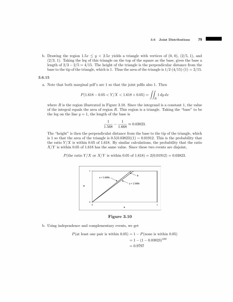
3.6 Joint Distributions 79
b. Drawing the region 1.5x ! y < 2.5x yields a triangle with vertices of (0, 0), (2/5, 1), and(2/3, 1). Taking the leg of this triangle on the top of the square as the base, gives the base alength of 2/3# 2/5 = 4/15. The height of the triangle is the perpendicular distance from thebase to the tip of the triangle, which is 1. Thus the area of the triangle is 1/2·(4/15)·(1) = 2/15.
3.6.15
a. Note that both marginal pdf’s are 1 so that the joint pdfis also 1. Then
P (1.618# 0.05 < Y/X < 1.618 + 0.05) =
66
R1 dy dx
where R is the region illustrated in Figure 3.10. Since the integrand is a constant 1, the valueof the integral equals the area of region R. This region is a triangle. Taking the “base” to bethe leg on the line y = 1, the length of the base is
1
1.568# 1
1.668$ 0.03823.
The “height” is then the perpendiculat distance from the base to the tip of the triangle, whichis 1 so that the area of the triangle is 0.5(0.03823)(1) = 0.01912. This is the probability thatthe ratio Y/X is within 0.05 of 1.618. By similar calculations, the probability that the ratioX/Y is within 0.05 of 1.618 has the same value. Since these two events are disjoint,
P (the ratio Y/X or X/Y is within 0.05 of 1.618) = 2(0.01912) = 0.03823.
0
1
0 1
y
x
y = 1.568x
y = 1.668xR
Figure 3.10
b. Using independence and complementary events, we get
P (at least one pair is within 0.05) = 1# P (none is within 0.05)
= 1# (1# 0.03823)100
= 0.9797

80 CHAPTER 3 Continuous Random Variables
c. Since the probability in part b. is so large, finding at least one pair of measurements that is“close” to the Golden Ratio is not unusual, even if the measurements are independent. Thismakes the claim somewhat questionable.
3.7 Functions of Independent Random Variables
3.7.1 By the definition of the expected value of a function of random variables, the expected valuesare
a. E [X + Y ] =
6 1
0
6 1
0(x+ y)6xy2 dy dx = 17/12,
b. E [X] =
6 1
0
6 1
0x6xy2 dy dx = 2/3,
c. E [Y ] =
6 1
0
6 1
0y6xy2 dy dx = 3/4, and
d. E,X2 + Y
-=
6 1
0
6 1
0
!x2 + y
"6xy2 dy dx = 5/4.
3.7.2 By the definition of the expected value of a function of random variables, the expected valuesare
a. E [2X + Y ] =
6 2
0
6 x
0(2x+ y)(1/2) dy dx = 10/3,
b. E,3X2 + Y 3
-=
6 2
0
6 x
0
!3x2 + y3
"(1/2) dy dx = 34/5, and
c. E [|Y #X|] = E [X # Y ] =
6 2
0
6 x
0(x# y)(1/2) dy dx = 2/3 since X > Y.
3.7.3 We the region 0 ! x ! 15, 0 ! y ! 15 into two sub-regions as shown in Figure 3.11. So that
E [|X # Y |] =6 15
0
6 x
0(x# y)(1/15)2 dy dx+
6 15
0
6 15
x(y # x)(1/15)2 dy dx = 75/2 + 5/2 = 5
3.7.4 The marginal pdf’s are fX(x) = 1/8 and fY (y) = 1/10 so that the joint pdf is 1/80 and
E,X2Y + 3
-=
6 10
2
6 20
10
!x2y + 3
"(1/80) dy dx = 623.
3.7.5 The joint pdf of X and $ is
f(x, &) = fX(x)f!(&) =4
!, 0 < x < 1/2, 0 < & < !/2.
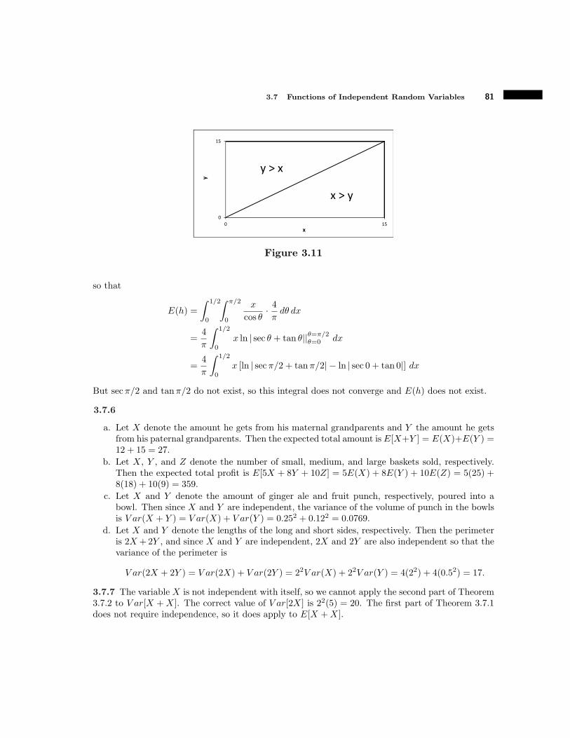
3.7 Functions of Independent Random Variables 81
0
15
0 15
y
x
x > y
y > x
Figure 3.11
so that
E(h) =
6 1/2
0
6 !/2
0
x
cos &· 4!d& dx
=4
!
6 1/2
0x ln | sec & + tan &||%=!/2
%=0 dx
=4
!
6 1/2
0x [ln | sec!/2 + tan!/2|# ln | sec 0 + tan 0|] dx
But sec!/2 and tan!/2 do not exist, so this integral does not converge and E(h) does not exist.
3.7.6
a. Let X denote the amount he gets from his maternal grandparents and Y the amount he getsfrom his paternal grandparents. Then the expected total amount is E[X+Y ] = E(X)+E(Y ) =12 + 15 = 27.
b. Let X, Y , and Z denote the number of small, medium, and large baskets sold, respectively.Then the expected total profit is E[5X + 8Y + 10Z] = 5E(X) + 8E(Y ) + 10E(Z) = 5(25) +8(18) + 10(9) = 359.
c. Let X and Y denote the amount of ginger ale and fruit punch, respectively, poured into abowl. Then since X and Y are independent, the variance of the volume of punch in the bowlsis V ar(X + Y ) = V ar(X) + V ar(Y ) = 0.252 + 0.122 = 0.0769.
d. Let X and Y denote the lengths of the long and short sides, respectively. Then the perimeteris 2X +2Y , and since X and Y are independent, 2X and 2Y are also independent so that thevariance of the perimeter is
V ar(2X + 2Y ) = V ar(2X) + V ar(2Y ) = 22V ar(X) + 22V ar(Y ) = 4(22) + 4(0.52) = 17.
3.7.7 The variable X is not independent with itself, so we cannot apply the second part of Theorem3.7.2 to V ar[X +X]. The correct value of V ar[2X] is 22(5) = 20. The first part of Theorem 3.7.1does not require independence, so it does apply to E[X +X].
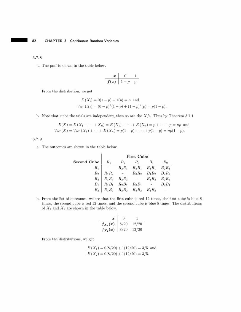
82 CHAPTER 3 Continuous Random Variables
3.7.8
a. The pmf is shown in the table below.
x 0 1
f(x) 1# p p
From the distribution, we get
E (Xi) = 0(1# p) + 1(p) = p and
V ar (Xi) = (0# p)2(1# p) + (1# p)2(p) = p(1# p).
b. Note that since the trials are independent, then so are the Xi’s. Thus by Theorem 3.7.1,
E(X) = E (X1 + · · ·+Xn) = E (X1) + · · ·+ E (Xn) = p+ · · ·+ p = np and
V ar(X) = V ar (X1) + · · ·+ E (Xn) = p(1# p) + · · ·+ p(1# p) = np(1# p).
3.7.9
a. The outcomes are shown in the table below.
First Cube
Second Cube R1 R2 R3 B1 B2
R1 - R2R1 R3R1 B1R1 B2R1
R2 R1R2 - R3R2 B1R2 B2R2
R3 R1R3 R2R3 - B1R3 B2R3
B1 R1B1 R2B1 R3B1 - B2B1
B2 R1B2 R2B2 R3B2 B1B2 -
b. From the list of outcomes, we see that the first cube is red 12 times, the first cube is blue 8times, the second cube is red 12 times, and the second cube is blue 8 times. The distributionsof X1 and X2 are shown in the table below.
x 0 1
fX1(x) 8/20 12/20
fX2(x) 8/20 12/20
From the distributions, we get
E (X1) = 0(8/20) + 1(12/20) = 3/5 and
E (X2) = 0(8/20) + 1(12/20) = 3/5.

3.7 Functions of Independent Random Variables 83
c. Note thatE(X) = E (X1 +X2) = E (X1) + E (X2) = 3/5 + 3/5 = 6/5.
d. The correct formula is E(X) = nN1/ (N1 +N2).
3.7.10 Note that P (X > Y ) = P (X # Y > 0). But the variable X # Y is
N!965# 995, 192 + 312
"= N(#30, 1322)
so that
P (X # Y > 0) = P
#Z >
0# (#30)/1322
$= P (Z > 0.83) = 0.2033.
3.7.11
a. Let Yi denote the weight of the ith “3-pound” package selected, i = 1, 2. Then each Yi isN!3.11, 0.092
". Then with Xi as defined in the example, we want to find
P (X1 + · · ·+X6 > Y1 + Y2) = P (X1 + · · ·+X6 # Y1 # Y2 > 0).
But this random variable is
N!6(1.05)# 2(3.11), 6(0.052) + 2(#1)2(0.092)
"= N(0.08, 0.0312)
so that
P (X1 + · · ·+X6 # Y1 # Y2 > 0) = P
#Z >
0# 0.08/0.0312
$= P (Z > #0.45) = 0.6736.
b. Generalizing the calculations in part a., the variable T1 # T2 is
N!3n(1.05)# n(3.11), 3n(0.052) + n(#1)2(0.092)
"= N(0.04n, 0.0156n)
so that
P (T1 # T2 > 0) = P
#Z >
0# 0.04n/0.0156n
$$ P (Z > #0.32
/n).
c. As n 1 0, #0.32/n 1 #0 so that P (Z > #0.32
/n) 1 1. They would want to buy the
1-pound packages.d. Generalizing the calculations in part b., the variable T1 # T2 is
N!3nµX # nµY , 3n#
2X + n#2
Y
"
so that
P (T1 # T2 > 0) = P
4Z >
0# (3nµX # nµY )/3n#2
X + n#2Y
5
The value of this probability is broken down into three cases:
84 CHAPTER 3 Continuous Random Variables
(a) If 3µX = µY , then this z-score is 0 so the probability is 0.5.
(b) If 3µX > µY , then this z-score is negative, so the probability 1 1 as n 1 0.
(c) If 3µX < µY , then this z-score is positive, so the probability 1 0 as n 1 0.
3.7.12 Let Y denote the weight of the “3-pound” package. Then the weight of one of the bagsmade from this package is Y/3. If X denotes the weight of a randomly chosen “1-pound” package,we want to find P (Y/3 > X) = P (Y # 3X > 0). The distributions of X and Y are as given inExample 3.7.6 so that the distribution of Y # 3X is
N!1(3.11)# 3(1.05), 12(0.092) + (#3)2(0.052)+
"= N(#0.04, 0.0306)
and P (Y # 3X > 0) = P (Z > 0.23) = 0.4090.
3.7.13
a. The three packages do not have to weigh the same. Denoting the total weight as X1+X2+X3
allows the packages to have di!erent weights, but the same distribution. Denoting the totalweight as 3X means that the total weight is 3 times the weight of one package, implying thepackages all weigh the same.
b. The variance of 3X is 32(0.052) = 0.0225 while the variance of X1 +X2 +X3 is 12 · 0.052 +12(0.052)+12(0.052) = 0.0075. Thus the variance of 3X is three times as large as the varianceof X1 +X2 +X3.
c. Since 3X and X1 + X2 + X3 do not have the same variance, they do not have the samedistribution.
3.7.14 Note that P (W > 90) = P [(X + Y )/2 > 90] = P (X + Y > 180). But the variable X + Y is
N!85 + 80, 42 + 52
"= N(165, 41)
and P (X + Y > 180) = P (Z > 2.34) = 0.0096
3.7.15 Let Xi denote the length of the ith movie. Then the total length of the n movies isT = Xi + · · ·Xn. But each Xi is N
!110, 152
"so that the distribution of T is N
!110n, 152n
"and
P (T > 8 hours) = P (T > 480 min) = P
#Z >
480# 110n
15/n
$.
From Table C.1, we see that P (Z > #1.645) $ 0.95. Thus we need
480# 110n
15/n
< #1.645 % 110n# 24.675/n# 480 > 0.
Solving this inequality with the quadratic formula yields/n > 2.204 which means n > 4.85. Thus
he must rent at least 5 movies.
3.7.16 Since X and Y are independent, Theorem 3.7.5 tells us that X2 and Y 2 are also independentrandom variables. Then by Theorem 3.7.2,
V ar,X2 + Y 2
-= V ar
,X2-+ V ar
,Y 2-= 2 + 3 = 5.

3.8 The Central Limit Theorem 85
3.8 The Central Limit Theorem
3.8.1 Note that the sample mean X12 is N(0.920, 0.003/12) = N(0.920, 0.00025)
a. P!X12 < 0.915
"= P (Z < #0.32) = 0.3745
b. P!0.915 < X12 < 0.922
"= P (#0.32 < Z < 0.13) = 0.5517# 0.3745 = 0.1772
c. The sample mean being less than 0.920 simply means that when you add all the masses anddivide by 12, the result is less than 0.920. It does not mean that all the masses are less than0.920
3.8.2 Let X denote the IQ score of a randomly chosen person. Then X is N!100, 152
".
a. P (X > 110) = P (Z > 0.67) = 0.2514b. The sample mean X25 is N
!100, 152/25
"= N(100, 9) so that
P!X25 > 110
"= P (Z > 3.33) = 0.0004.
3.8.3 The sample mean X45 is N!16, 0.082/48
"= N(16, 0.000133) so that
P!X48 > 16.04
"= P (Z > 3.46) = 0.0003.
Since this probability is so small, the observed sample mean of x = 16.04 is very unlike to haveoccurred if µ = 16. This indicates that µ is probably greater than 16 meaning the bottles are filledwith an amount greater than 16.00 oz.
3.8.4 Since X is b(500, 1/5), the population mean and variance are µ = 500(1/5) = 100 and #2 =500(1/5)(4/5) = 80. Thus the sample mean X50 is approximately N (100, 80/50) = N(100, 1.6) sothat
P!X50 < 99
"$ P (Z < #0.79) = 0.2148.
3.8.5 Scores on a certain standardized test have a normal distribution with mean of µ = 1515 andvariance of #2 = 3002. A random sample of n scores is selected.
a. Note that Xn is N(1515, 3002/n). The calculations of the probabilities are summarized in thetable below.
n V ar!Xn
"z1 z2 P
!1510 < Xn < 1520
"
5 18000 -0.04 0.04 0.0320
50 1800 -0.12 0.12 0.0956
250 360 -0.26 0.26 0.2052
500 180 -0.37 0.37 0.2886
5000 18 -1.18 1.18 0.7620
b. The probability gets larger.c. Based on these calculations, it appears that lim
n"$P!µ# ' < Xn < µ+ '
"= 1.

86 CHAPTER 3 Continuous Random Variables
3.8.6 Note that Xn is N(172, 292/n). Then
P!Xn > 3500/n
"= P
#Z >
3500/n# 172
29//n
$.
From Table C.1, we see that P (Z > 2.325) $ 0.01. Thus we need
3500/n# 172
29//n
> 2.325 % 0 > 172n+ 67.425/n# 3500
This inequality is quadratic in/n. Solving this using the quadratic formula yields
/n < 4.319
so that n < 18.65. This means the largest value of n is 18. (Note: Another way to solve thisproblem is to calculate P
!Xn > 3500/n
"for di!erent values of n and find the largest such that the
probability is less than 0.01.)
3.8.7
a. Based on the given assumptions, X109 is N(98.6, 0.062/109) = N(98.6, 0.000033) so that
P!X109 < 98.3
"= P (Z < #9090) = 0.0000.
b. Since this probability is so small, the assumption that the mean body temperature of thepopulation of healthy adults is 98.6 (F is probably not correct.
3.8.8
a. Since Xn is approximately N!µ, #2/n
", its mgf is approximately
MX(t) = exp
Gµt+
!#2/n
"t2
2
H
By exercise 2.7.7, the mgf of Y = Xn # µ is approximately
MX(t) = exp {#µt} expGµt+
!#2/n
"t2
2
H= exp
G!#2/n
"t2
2
H
But this is the mgf of a random variable that is N!0, #2/n
". Thus Y approximately has this
distribution.b. Note that
P!µ# ' < Xn < µ+ '
"= P
!#' < Xn # µ < '
".
But by part a., the variable Xn # µ is approximately N!0, #2/n
"so that
P!#' < Xn # µ < '
"$ P
##'
#//n< Z <
'
#//n
$= P
##/n'
#< Z <
/n'
#
$.
As n 1 0, #/n'/# 1 #0 and
/n'/# 1 0 so that
P
##/n'
#< Z <
/n'
#
$1 1.

3.8 The Central Limit Theorem 87
3.8.9 We want to find P!#10 < X100 # µ < 10
". By exercise 3.8.8, the variable X100 # µ is
approximately N(0, 3252/100) = N(0, 1056.25) so that
P!#10 < X100 # µ < 10
"= P (#0.31 < Z < 0.31) = 0.2434.
3.8.10 We want to find n such that P!#50 < Xn # µ < 5
"" 0.95. By exercise 3.8.8, the variable
Xn # µ is approximately N(0, 3252/n) so that
P!#50 < Xn # µ < 50
"=
##50
325//n< Z <
50
325//n
$.
From Table C.1, we see that P (#1.96 < Z < 1.96) = 0.95. Thus we need
50
325//n> 1.96 % n > 162.3.
Thus the researcher needs a sample size of at least 163.
3.8.11
a. By section 3.3, the mean and variance are µ = #2 = 1. A typical graph of the exponential pdfis given in that section. This distribution is not anywhere “close” to normal.
b. The marginal pdf’s are fX1((x1) = e!x1 and fX2((x2) = e!x2 . Since X1 and X2 are indepen-dent, the joint pdf is f (x1, x2) = e!x1!x2 .
c. Note that since X2 < 1/2, and X1 and X2 cannot be negative, neither variable can be largerthan 1. Thus
P!X2 < 1/2
"= P [(X1 +X2) /2 < 1/2]
= P [X2 < 1#X1]
=
6 1
0
6 1!x1
0e!x1!x2 dx2 dx1 $ 0.2642
d. According to the central limit theorem, X2 is approximately N(1, 1/2) so that
P!X2 < 1/2
"$ P (Z < #0.71) = 0.2389.
This estimate is rather poor with a relative error of about 9.6%. This estimate is poor becausethe population distribution is not “close” to normal and the sample size is very small.
3.8.12 By the central limit theorem, Xn is approximately N!µX , #2
X/n"and Yn is approximately
N!µY ,#2
Y /n". By Theorem 3.7.4, the variable Dn = Xn # Yn is then approximately
N!µX # µY , 1
2#2X/n+ (#1)2#2
Y /n"= N
!µX # µY ,
!#2X + #2
Y
"/n".

88 CHAPTER 3 Continuous Random Variables
3.8.13 Let X30 and Y30 denote the sample means of the men and women, respectively. By exercise3.8.12, the variable Xn # Yn is approximately
N!69# 63.6,
!2.82/n+ 2.52
"/30"= N(5.4, 0.4697)
so thatP!5.25 < Xn # Yn < 5.75
"$ P (#0.22 < Z < 0.51) = 0.2821
3.8.14
a. limN"$
#1# n# 1
N # 1
$= 1
b. This limit tells us that the finite population correction is not necessary when n is very smallin comparison to the population size.
3.9 The Gamma and Related Distributions
3.9.1
a. W has a gamma distribution with parameters r = 2 and " = 10/60 = 1/6 so that its pdf is
f(w) =((1/6)2
(2# 1)!w2!1 e!(1/6)w =
w e!w/6
36for w > 0,
its mean is µ = 2/(1/6) = 12, and its variance is #2 = 2/(1/6)2 = 72.b. If the second call arrives before 8:15 AM, then W < 15, so
P (W < 15) =
6 15
0
w e!w/6
36dw = 0.7127.
c. If r = 8, then the pdf is
f(w) =((1/6)8
(8# 1)!w8!1 e!(1/6)w =
w7 e!w/6
68 · 7! for w > 0,
so that
P (W < 45) =
6 45
0
w7 e!w/6
68 · 7! dw = 0.4754.
3.9.2 Let W denote the wait time (in hours) until the second replacement of the batteries. ThenW has a gamma distribution with parameters r = 2 and " = 1/10 so that its pdf is
f(w) =((1/10)2
(2# 1)!w2!1 e!(1/10)w =
w e!w/10
100for w > 0.

3.9 The Gamma and Related Distributions 89
Now, the two sets of batteries last the entire trip if the time until the second replacement is greaterthan eight hours. Thus we need to know P (W > 8), so
P (W > 8) = 1# P (W < 8) = 1#6 8
0
w e!w/10
100dw = 0.8088.
3.9.3 By definition,
%(0.75) =
6 $
0y0.75!1 e!y dy $ 1.225.
Then, %(1.75) $ 0.75(1.225) = 0.919 and %(2.75) $ 1.75(0.919) = 1.608
3.9.4 a. P (X ! 25) = 0.95 b. P (X > 7.261) = 0.05 c. P (5.229 < X ! 8.547) = 0.09
3.9.5 LetW denote the wait time until the 10th customer arrives. ThenW has a gamma distributionwith parameters r = 10 and " = 1/2. But this is the same as a chi-square distribution with n = 20degrees of freedom. Thus using Table C.4, we find that
P (W < 34.17) = 0.975
.
3.9.6
a. P (T ! 2.447) = 0.975 b. P (T > 3.143) = 0.01
c. P (#1.943 < T ! 1.943) = 0.9 d. P (#3.707 < T ! 1.943) = 0.945
3.9.7 Notice that in f(t), the Student-t pdf, the only place t appears is in the denominator as t2.Replacing t with #t will not change the value of this term. So f(t) = f(#t) for any number ofdegrees of freedom n.
3.9.8 Note that by equation (3.7)
T 2 =Z2
C/n(3.1)
But Z2 is (2(1) and C is (2(n) so that T 2 fits the definition of a variable that has an F distributionwith 1 and n degrees of freedom as given in equation (3.8).
3.9.9
a. The graph is shown in Figure 3.12. We see that this is the same as a U(0, 1) distribution.b. The graphs are shown in Figure 3.12.c. If X has a beta distribution with a = 5 and b = 1, then its pdf is
f(x) =%(5 + 1)
%(5)%(1)x5!1(1# x)1!1 =
5!
4! · 0! x4(1# x)0 = 5x4
so that
P (X > 0.5) =
6 1
0.55x4 dx = 31/32 = 0.96875

90 CHAPTER 3 Continuous Random Variables
0
0.5
1
1.5
2
2.5
3
0 0.2 0.4 0.6 0.8 1
y
x
a = 1, b = 3
a = 2, b = 5
a = 2, b = 2
a = 1, b = 1
Figure 3.12
3.9.10 By the definition of expected value,
E(X) =
6 $
0xk
"
=x"
>k!1e!(x/")k dx =
6 $
0
x
"e!(x/")kk
=x"
>k!1dx.
Now let y = (x/")k. Then when x = 0, y = 0; when x 1 0, y 1 0;
dy = k=x"
>k!1 1
"dx and
x
"= y1/k.
By substitution and the definition of %(t),
E(X) = "
6 $
0y1/k e!y dy = "
6 $
0y(1+1/k)!1 e!y dy = "% (1 + 1/k) .
3.9.11 The (2 distribution is a special case of the gamma distribution where " = 1/2 and r = n/2.Thus
E(X) =r
"=
n/2
1/2= n.
3.9.12 The mgf of X is MX(t) = (1 # 2t)!n/2 and the mgf of Y is MY (t) = (1 # 2t)!m/2. ByTheorem 3.7.3, the mgf of W is
MW (t) = MX(t) ·MY (t) = (1# 2t)!n/2 · (1# 2t)!m/2 = (1# 2t)(!n!m)/2.
But this is the mgf of a random variable that is (2(n+m). Thus W has this distribution.
3.9.13 We let W = W1 +W2 + · · · +Wn as in Example 3.9.2 where each Wi has an exponentialdistribution with parameter ". By the calculations immediately following Example 3.3.5, the mgf ofeach Wi is "/("# t) for t < ". By Theorem 3.7.3, since these n variables are mutually independent,the mgf of W is the product of their mgf’s so that
MW (t) =
#"
"# t
$n
for t < ".

3.9 The Gamma and Related Distributions 91
3.9.14 By the definition of the m.g.f, the mgf of a random variable W with a gamma distributionand parameters " and r is
MW (t) = E,eWt
-=
6 $
0ewt "r
%(r)wr!1 e!"w dw =
"r
%(r)
6 $
0wr!1 e(t!")w dw.
Notice that for this integral to converge, we need t # " < 0 % t < ". Now let y = (" # t)w.Then when w = 0, y = 0; when w 1 0, y 1 0 (since "# t > 0);
w =y
"# tand dw =
dy
"# t.
By substitution and the definition of %(t),
MW (t) ="r
%(r)
6 $
0wr!1 e(t!")w dw
="r
%(r)
6 $
0
yr!1
("# t)r!1e!y dy
"# t
="r
%(r)("# t)r
6 $
0yr!1 e!y dy
="r
%(r)("# t)r%(r)
="r
("# t)rfor t < ".
3.9.15 a. P (F ! 1.88) = 0.975 b. P (F > 2.12) = 0.01 c. P (1.70 ! F ! 2.12) = 0.04
3.9.16 a. P (F > 4.95) = 0.05 b. P (F ! 10.67) = 0.99 c. P (F > 10.67(F ! 4.95) = 0.01+0.95 =0.96
3.9.17 In Figure 3.22, we see that the density curve is very tall over the interval (0.5, 1.5] but veryshort over (2, 4]. Geometrically, we also see that there is more area under the curve over the firstinterval than the second. Thus P (0.5 < F ! 1.5) > P (2 < F ! 4).
3.9.18 By definition of the F -distribution with n and d degrees of freedom, U is (2(n) and V is(2(d) and they are independent. Then
1
F=
V/d
U/n
so that 1/F has an F -distribution with d and n degrees of freedom by definition.
3.9.19
a. Let u =/
2! so that/
2du = y!1/2dy and
%
#1
2
$=
6 $
0y!1/2e!ydy =
6 $
0
/2e!u2/2du = 2
/!
6 $
0
1/2!
e!u2/2du
= 2/! · 1
2=
/!.

92 CHAPTER 3 Continuous Random Variables
b. From exercise 3.5.9, the pdf of X is
f(x) =1/2!x
e!x/2.
But the pdf of a gamma distribution with " = r = 1/2 is
f(x) =(1/2)1/2
%(1/2)x!1/2 e!x/2 =
(1/2)1/2/!
x!1/2 e!x/2 =1/2!x
e!x/2
which is the same as the pdf of X. Thus X has a gamma distribution with " = r = 1/2. Sincethis is the case, the mgf of X is
M(t) = (1# t/(1/2))!1/2 = (1# 2t)!1/2.
c. By Theorem 3.7.5, the variables Y 21 , Y
22 , . . . , Y
2n are independent. Thus X is the sum of
independent random variables, each with mgf M(t) = (1# 2t)!1/2. Hence by Theorem 3.7.3,the mgf of X is
MX(t) = (1# 2t)!1/2 · · · (1# 2t)!1/2
& '( )n times
= (1# 2t)!n/2.
d. The mgf in part c. is exactly that of a random variable with a gamma distribution with" = 1/2 and r = n/2. Thus X has the pdf given in Theorem 3.9.1.
3.10 Approximating the Binomial Distribution
3.10.1 People often travel in groups, such as families, and thus arrive together. So the arrivals arenot mutually independent, but independence is a reasonable simplifying assumption.
3.10.2 Let Y be N(950(0.35), 950(0.35)(1# 0.35)) = N(332.5, 216.125).
a. P (310 ! X ! 350) $ P (310 # 0.5 < Y ! 350 + 0.5) = P (#1.56 < Z ! 1.22) = 0.8888 #0.0594 = 0.8294
b. P (X ! 315) $ P (Y ! 315 + 0.5) = P (Z ! #1.16) = 0.1230
c. P (340 ! X) $ P (340# 0.5 < Y ) = P (0.48 < Z) = 0.3156
3.10.3 Suppose X is b(75, 0.02).
a. Note that np = 1.5 and n(1 # p) = 73.5. Since np < 5, the rule-of-thumb indicates that wecannot use equation (3.9) to approximate values of the probability of X.
b. Using software, P (X ! 1) = 0.5561.

3.10 Approximating the Binomial Distribution 93
c. Let Y be N(75(0.02), 75(0.02)(1# 0.02)) = N(1.5, 1.47). Then according to equation (3.9),
P (X ! 1) $ P (Y ! 1 + 0.5) = P (Z ! 0) = 0.5.
This approximation has a relative error of 0.0561/0.5561 $ 10%, so this is not a good approx-imation.
3.10.4 Let X denote the number of gamblers out of 5,000 that win. Then X is b(5, 000, 1/38). LetY be N(5000(1/38), 5000(1/38)(1 # 1/38)) = N(131.58, 128.12). Then the probability that morethan 140 of them win is
P (140 < X) = P (141 ! X) $ P (141# 0.5 < Y ) = P (0.79 < Z) = 0.2148.
3.10.5
a. Let X denote the number of voters out of 825 that actually did vote for the proposition. ThenX is b(825, 0.4). Let Y be N(825(0.4), 825(0.4)(1#0.4)) = N(330, 198). Then the probabilitythat more than 429 of them actually did vote for the proposition is
P (429 < X) = P (430 ! X) $ P (430# 0.5 < Y ) = P (7.07 < Z) = 0.0000.
b. The fact that this probability is so small indicates that observing 429 or more that actuallydid vote for the proposition is extremely unusual, assuming the people are being honest. Thissuggests that people are not honestly responding to the survey.
3.10.6 Let X denote the number of points selected such that x ! y out of 500. Figure 3.13 showsthe rectangle 0 ! x ! 1, 0 ! y ! 2 and the portion in which x ! y. We see that the total areaof the region is 2 and the area of the portion in which x ! y is 2 # (1/2)(1)(1) = 3/2. Thus theprobability of selecting a point such that x ! y is (3/2)/2 = 3/4. This means that X is b(500, 0.75).Let Y be N(500(0.75), 500(0.75)(1# 0.75)) = N(375, 93.75). Then the probability that for 365 ormore of these points, x ! y, is
P (365 ! X) $ P (365# 0.5 < Y ) = P (#1.08 < Z) = 0.8599.
3.10.7 Let X denote the number of students out of n that regularly use credit cards. Then X isb(n, 0.25). Let Y be N(n(0.25), n(0.25)(1 # 0.25)) = N(0.25n, 0.1875n). We want to find n suchthat
0.95 < P (50 ! X) $ P (50# 0.5 < Y ) = P
#49.5# 0.25n/
0.1875n< Z
$.
From Table C.1, we see that P (#1.645 < Z) $ 0.95. Thus we want
49.5# 0.25n/0.1875n
< #1.645 % 0 < 0.25n# 0.7123/n# 49.5.
This inequality is quadratic in/n. Solving it with the quadratic formula yields
/n > 15.57 so that
n > 242.4. Thus the researcher needs a sample size of at least 243.

94 CHAPTER 3 Continuous Random Variables
0
1
2
0 1
y
x
x < y
Figure 3.13
3.10.8
a. Note that X is b(n, 1/2) so that µ = n/2 and #2 = n/4.b. Note that
P
#7777X
n# 1
2
7777 < $
$= P
=777X # n
2
777 < n$>
> 1# n/4
(n$)2by Chevyshev’s inequality
= 1# 1
4n$2.
c. By elementary calculus, limn"$!1# 1
4n#2
"= 1. Note that X/n is the relative frequency
of tails and |X/n # 1/2| is the di!erence between the relative frequency and the theoreticalprobability and $ is an upper bound on this di!erence. The fact that this limit equals 1 meansthat we can make this di!erence as small as we want, with probability as close to 1 as we want,by choosing a large enough value of n. In simpler terms, this means that as n gets larger, therelative frequency gets closer to the theoretical probability.
Chapter 4
Statistics
4.1 What is Statistics?
4.1.1
a. Population - All voters in the city, Sample - 50 voters. This is biased because not everyone inthe city lives in a house with a 3-car garage, so the sample is not representative of the entirepopulation.
b. Population - All students at the university, Sample - Students in the 4 classes. This is biasedbecause the sample includes only math students, so the sample is not representative of theentire population.
c. Population - All students at the university, Sample - 50 students selected from the studentdirectory. This is not biased because the students were randomly selected from the population.
d. Populations - All potatoes of the 3 varieties, Samples - 3 bags of potatoes. These samplesare biased because the samples are not randomly chosen from the respective populations. Allpotatoes in a single bag probably came from the same crop, so they are not representative oftheir population.
e. Population - All fellow students, Sample - 15 friends. This is biased because he asked only hisfriends, so the sample is not representative of the entire population.
f. Population - All fiber optic cable manufactured in a day, Sample - Selected pieces of cable.This is not biased because the pieces are selected throughout the day.
4.1.2
a. Statistic - The biologist surely did not observe all the ghost crabs on the beach.b. Parameter - All the names in the book were surveyed.
95

96 CHAPTER 4 Statistics
c. Parameter - All of the records were surveyed.d. Statistic - The mother surely did not observe all of the teenagers in the mall.e. Statistic - The o"cer surely did not survey every mile of highway in the region. The percentage
is based on what was actually observed.
4.1.3 a. Quantitative, continuous; b. Qualitative; c. Quantitative, discrete; d. Quantitative,continuous; e. Quantitative, discrete
4.1.4 a. Discrete, b. Continuous, c. Continuous, d. Discrete, e. Continuous
4.1.5 a. Nominal, b. Interval, c. Ratio, d. Ratio, e. Ordinal
4.1.6 a. Ratio, b. Nominal, c. Interval, d. Nominal, e. Interval
4.1.7 a. Observational, b. Experiment, c. Experiment, d. Observational, e. Experiment
4.1.8 a. Convenience, b. Systematic, c. Voluntary response, d. Cluster, e. Stratified
4.1.9
a. A drug may work better for some types of cancer than others. The factor of type of cancerneeds to be accounted for.
b. The individual professors could influence homework scores, so there are nuisance variables notaccounted for.
c. One factor not accounted for is the surface area of the parachute.d. The researcher needs to take into account lifestyle, income, diet, and other habits when trying
to determine “causes” of good health.e. Di!erent gardners grow tomatoes in di!erent ways. Factors such as amount of irrigation,
amount and type of fertilizer, soil type, and others are di!erent from gardner to gardner.These factors need to be accounted for.
4.1.10
a. Since all the candies are mixed, this is a simple random sample.
b. Since the row is randomly chosen, the sample is random. But only groups of students who sitin the same row can be selected, so the sample is not a simple random sample.
c. Since the people are randomly chosen and the population is half male and half female, everymember has an equal probability of being selected so the sample is random. However, wecould not, for instance, get a sample of 25 males and 75 females, so the sample is not a simplerandom sample.
d. There is nothing random about this sample at all, so it is neither a random sample nor asimple random sample.
4.1.11 No. Temperatures are at the interval level of measurement. Although there is a zero startingpoint, 0(F does not mean no temperature, so ratios such as “twice as hot” are meaningless.
4.1.12 Label the dice as first, second, and third. Roll the 3 dice. The number on the first die givesthe room number, the second die gives the row number, and the third gives the student number.Repeat this 20 times.
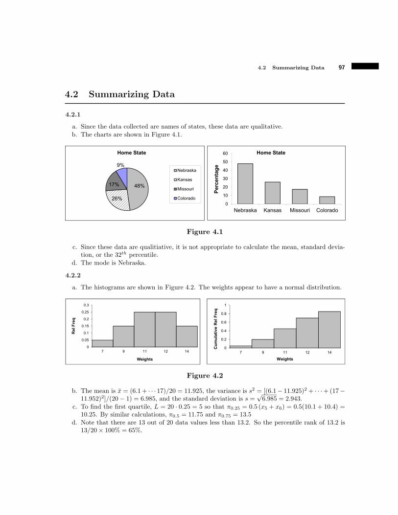
4.2 Summarizing Data 97
4.2 Summarizing Data
4.2.1
a. Since the data collected are names of states, these data are qualitative.b. The charts are shown in Figure 4.1.
48%
26%
17%
9%
Home State
Nebraska
Kansas
Missouri
Colorado0
10
20
30
40
50
60
Nebraska Kansas Missouri ColoradoPe
rcen
tage
Home State
Figure 4.1
c. Since these data are qualitiative, it is not appropriate to calculate the mean, standard devia-tion, or the 32th percentile.
d. The mode is Nebraska.
4.2.2
a. The histograms are shown in Figure 4.2. The weights appear to have a normal distribution.
0
0.05
0.1
0.15
0.2
0.25
0.3
7 9 11 12 14
Rel
Fre
q
Weights
0
0.2
0.4
0.6
0.8
1
7 9 11 12 14
Cum
ulat
ive
Rel
Fre
q
Weights
Figure 4.2
b. The mean is x = (6.1+ · · · 17)/20 = 11.925, the variance is s2 = [(6.1# 11.925)2 + · · ·+ (17#11.952)2]/(20# 1) = 6.985, and the standard deviation is s =
/6.985 = 2.943.
c. To find the first quartile, L = 20 · 0.25 = 5 so that !0.25 = 0.5 (x5 + x6) = 0.5(10.1 + 10.4) =10.25. By similar calculations, !0.5 = 11.75 and !0.75 = 13.5
d. Note that there are 13 out of 20 data values less than 13.2. So the percentile rank of 13.2 is13/20& 100% = 65%.

98 CHAPTER 4 Statistics
4.2.3
a. The mean is x = (0.783 + · · · 0.976)/30 = 0.890, the variance is s2 = [(0.783 # 0.89)2 +· · · (0.976# 0.89)2]/(30# 1) = 0.00208, and the standard deviation is s =
/0.00208 = 0.0456
b. The histograms are shown in Figure 4.3. The weights appear to have a normal distribution.
00.050.1
0.150.2
0.250.3
0.35
0.78 0.81 0.84 0.87 0.90 0.93 0.96 0.99
Rel F
req
Weights
0
0.2
0.4
0.6
0.8
1
1.2
0.78 0.81 0.84 0.87 0.90 0.93 0.96 0.99
Cum
ulat
ive
Rel F
req
Weights
Figure 4.3
4.2.4
a. The mean is x = (2.09 + · · · 3.26)/30 = 2.621, the variance is s2 = [(2.08 # 2.621)2 + · · · +(3.26# 2.621)2]/(30# 1) = 0.0858, and the standard deviation is s =
/0.0858 = 0.2930.
b. The histograms are shown in Figure 4.4. The percent shrink appears to have a normal distri-bution.
00.050.1
0.150.2
0.250.3
0.350.4
0.450.5
2.13 2.38 2.63 2.88 3.13 3.38
Rel F
req
Percent Shrink
0
0.2
0.4
0.6
0.8
1
1.2
2.13 2.38 2.63 2.88 3.13 3.38
Cum
ulat
ive
Rel F
req
Percent Shrink
Figure 4.4
c. By part a., µ $ x = 2.621 and # $ s = 0.293 so that the range is approximately
(2.621# 3(0.293), 2.621 + 3(0.293)) % (1.742, 3.5) .
d. Yes, the range in part c. falls between 1% and 4%.
4.2.5
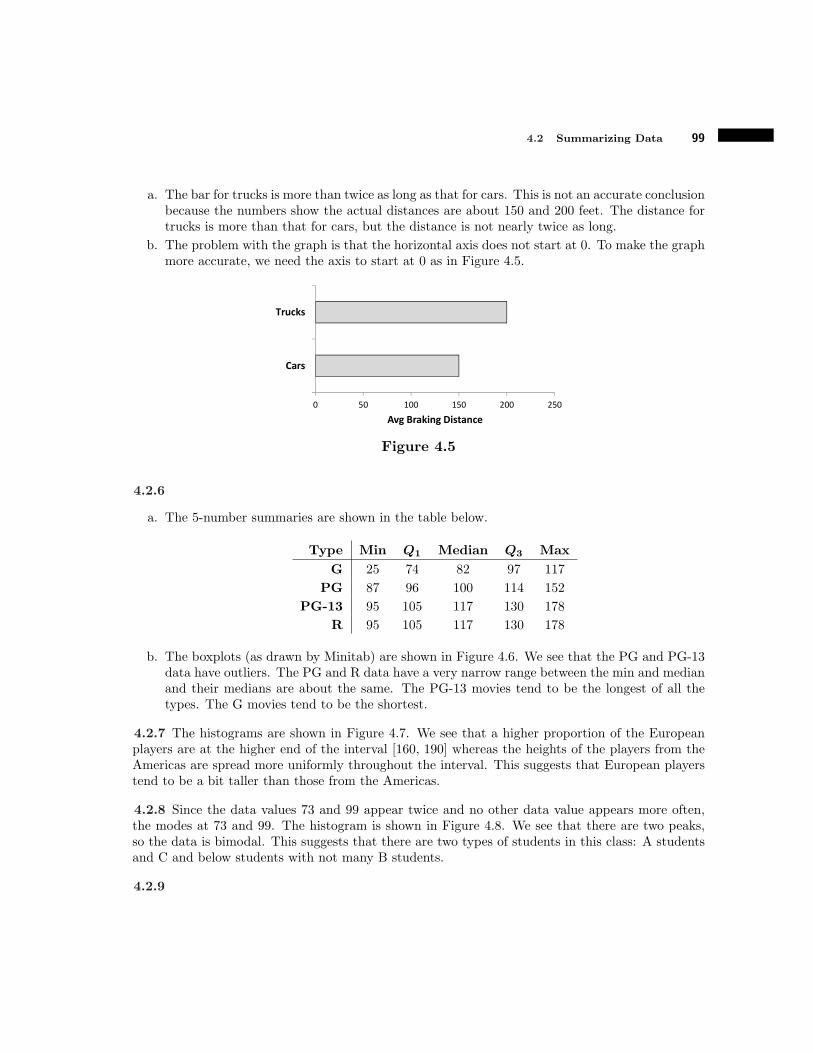
4.2 Summarizing Data 99
a. The bar for trucks is more than twice as long as that for cars. This is not an accurate conclusionbecause the numbers show the actual distances are about 150 and 200 feet. The distance fortrucks is more than that for cars, but the distance is not nearly twice as long.
b. The problem with the graph is that the horizontal axis does not start at 0. To make the graphmore accurate, we need the axis to start at 0 as in Figure 4.5.
0 50 100 150 200 250
Cars
Trucks
Avg Braking Distance
Figure 4.5
4.2.6
a. The 5-number summaries are shown in the table below.
Type Min Q1 Median Q3 Max
G 25 74 82 97 117
PG 87 96 100 114 152
PG-13 95 105 117 130 178
R 95 105 117 130 178
b. The boxplots (as drawn by Minitab) are shown in Figure 4.6. We see that the PG and PG-13data have outliers. The PG and R data have a very narrow range between the min and medianand their medians are about the same. The PG-13 movies tend to be the longest of all thetypes. The G movies tend to be the shortest.
4.2.7 The histograms are shown in Figure 4.7. We see that a higher proportion of the Europeanplayers are at the higher end of the interval [160, 190] whereas the heights of the players from theAmericas are spread more uniformly throughout the interval. This suggests that European playerstend to be a bit taller than those from the Americas.
4.2.8 Since the data values 73 and 99 appear twice and no other data value appears more often,the modes at 73 and 99. The histogram is shown in Figure 4.8. We see that there are two peaks,so the data is bimodal. This suggests that there are two types of students in this class: A studentsand C and below students with not many B students.
4.2.9

100 CHAPTER 4 Statistics
Dat
a
RPG-13PGG
200
150
100
50
Boxplot of G, PG, PG-13, R
Figure 4.6
0
0.1
0.2
0.3
0.4
0.5
167.5 172.5 177.5 182.5 187.5
Rel F
req
Height of European Players
0
0.1
0.2
0.3
0.4
0.5
167.5 172.5 177.5 182.5 187.5
Rel F
req
Height of Players from the Americas
Figure 4.7
0
0.1
0.2
0.3
0.4
55.0 65.0 75.0 85.0 95.0
Rel F
req
Score
Figure 4.8
a. Yes. If a set of data contains negative values, then it is possible for the mean to be negative.
b. No. Since the variance is the sum of squares, it can never be negative.
c. Yes. Consider the data set {#1, 0, 1}. Its mean is 0 and its variance is 1, so it is possible thatthe variance can be larger than the mean.
d. No. By definition !0.25 is a value that is greater than about 25% of the data values while !0.75

4.2 Summarizing Data 101
is greater than about 50%. So !0.25 cannot be larger than !0.75. They could be eqaul if thedata set contains some repeated data values.
e. No. Consider the data set {1, 2, 3, 10}. The mean is 4 which is greater than more than halfthe data values.
f. No. Consider the data set {1, 1, 1, 1}. The mean is 1 which is not greater than any of thedata values.
4.2.10
a. The min and max of this data are 0 and 7.3, so midrange = (7.3# 0)/2 = 3.65.b. The median is 1.8. This is much less than the midrange.c. The phrase “in the middle, halfway between the min and max“ is describing the midrange.
4.2.11 If x is a value of a normally distributed random variable with mean µ and standard deviation#, in section 3.4 we defined the z-score of x to be z = (x # µ)/#. Now, if x is a data value from aset of data with mean x and standard deviation s, we define the z-score of x to be
z =x# x
s.
The z-score is a measure of how far x is from the mean.
a. If x > x, then x # x > 0 so that z > 0 since s > 0. A similar argument shows that if x < x,then z < 0
b. If x = (x+ n · s) where n is any number, then
z =x# x
s=
(x+ n · s)# x
s=
n · ss
= n.
If x1 is “further” from the mean than x2, then we could say x1 = x+n1 · s and x1 = x+n2 · sfor some numbers n1 and n2 such that |n1| > |n2| so that how does the the magnitude of thez-score of x1 is greater than that of x2?
c. Bob’s z-score is z = (80 # 90)/5 = #2 and Joe’s is z = (50 # 55)/10 = #0.5. Since Joe’sz-score is smaller in magnitude, Joe’s test score is relatively closer to the mean than Bob’stest score. So Joe did relatively better.
4.2.12 We can freely choose 4 of the data values. Let S denote the sum of these values. The lastdata value, call it x must be chosen such that x = (S + x)/5 = 3.2. There is only one solution tothis equation, so there is only one possible value for x. In general, if we want a sample of n datavalues with a specified mean, we can freely choose n# 1 of them.
4.2.13
a. The histograms are shown in Figure 4.9.b. We see that Class 1 has many data values equal to the mean and not many very far from
the mean, so it’s standard deviation, or “average distance from the mean,” is relatively small.Class 2 exhibits the exact opposite, so its standard deviation is relatively large. Class 3 hassome data values close to the mean and some far from the mean, so its standard deviation isbetween that of classes 1 and 3.

102 CHAPTER 4 Statistics
0
0.1
0.2
0.3
0.4
0.5
2 3 4 5 6 7
Rel F
req
Score
Class 1
0
0.1
0.2
0.3
2 3 4 5 6 7
Rel F
req
Score
Class 2
0
0.1
0.2
0.3
0.4
0.5
2 3 4 5 6 7
Rel F
req
Score
Class 3
Figure 4.9
c. The sample standard deviations are Class 1: 1.095, Class 2: 1.67, Class 3: 1.26. This agreeswith the conclusions in part b.
4.2.14 The mean, median, mode and skewness of the data sets are summarized in the table below,and the histograms are shown in Figure 4.10. We see that set 1 is skewed right, set 2 is symmetric,and set 3 is skewed left. Skewed right corresponds to a positive skewness, skewed left to a negativeskewness, and symmetric to a skewness of 0.
Mean Median Mode Skewness
Set 1 2.91 3 2 0.86
Set 2 5 5 5 0
Set 3 5 5 6 -1.45
4.2.15
a. The calculations of the sample kurtoses are summarized in the table below. Note that n = 11for each data set. The histograms are shown in Figure 4.11.
x.
(xi ! x)4.
(xi ! x)2 Kurtosis
Set 1 5 2 2 5.00
Set 2 4 36 12 0.42
Set 3 3 198 30 -0.13
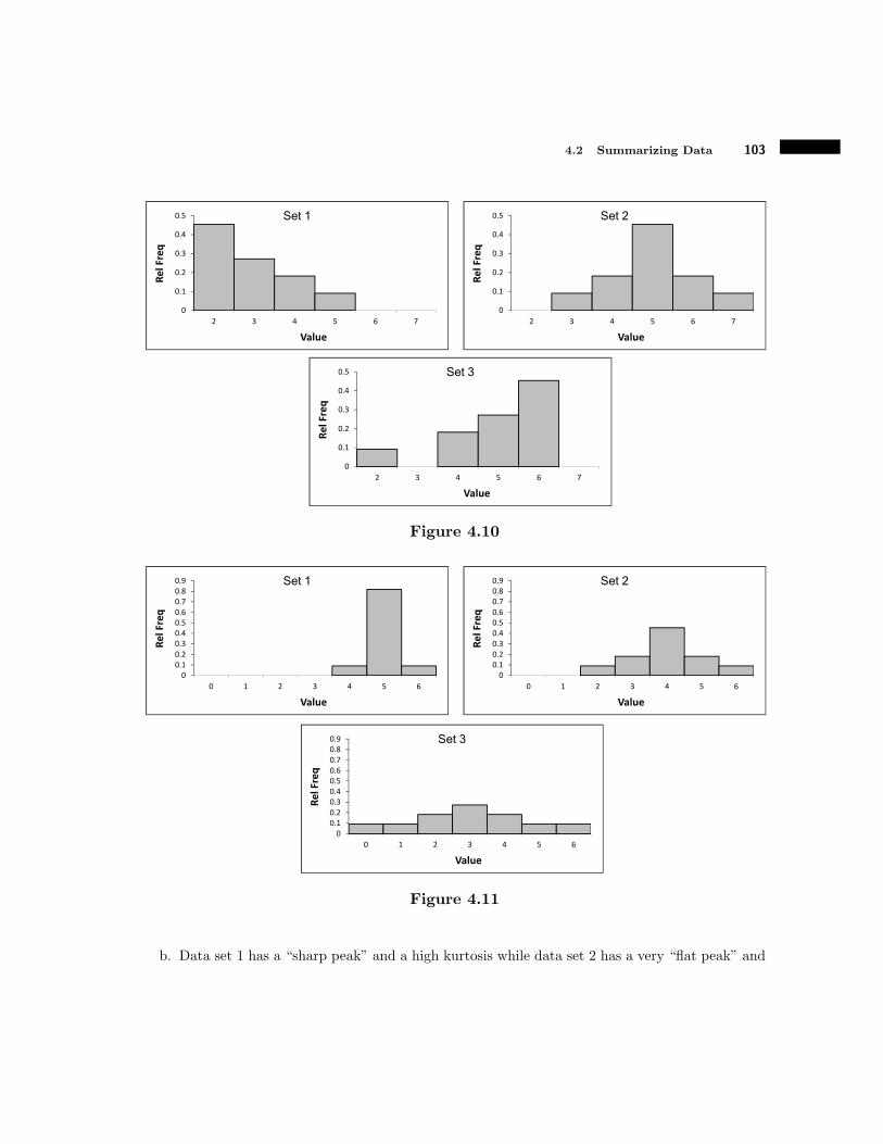
4.2 Summarizing Data 103
0
0.1
0.2
0.3
0.4
0.5
2 3 4 5 6 7
Rel F
req
Value
Set 1
0
0.1
0.2
0.3
0.4
0.5
2 3 4 5 6 7
Rel F
req
Value
Set 2
0
0.1
0.2
0.3
0.4
0.5
2 3 4 5 6 7
Rel F
req
Value
Set 3
Figure 4.10
00.10.20.30.40.50.60.70.80.9
0 1 2 3 4 5 6
Rel F
req
Value
Set 1
00.10.20.30.40.50.60.70.80.9
0 1 2 3 4 5 6
Rel F
req
Value
Set 2
00.10.20.30.40.50.60.70.80.9
0 1 2 3 4 5 6
Rel F
req
Value
Set 3
Figure 4.11
b. Data set 1 has a “sharp peak” and a high kurtosis while data set 2 has a very “flat peak” and
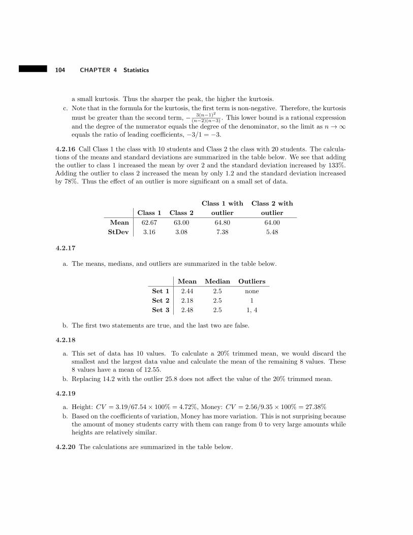
104 CHAPTER 4 Statistics
a small kurtosis. Thus the sharper the peak, the higher the kurtosis.
c. Note that in the formula for the kurtosis, the first term is non-negative. Therefore, the kurtosis
must be greater than the second term, # 3(n!1)2
(n!2)(n!3) . This lower bound is a rational expressionand the degree of the numerator equals the degree of the denominator, so the limit as n 1 0equals the ratio of leading coe"cients, #3/1 = #3.
4.2.16 Call Class 1 the class with 10 students and Class 2 the class with 20 students. The calcula-tions of the means and standard deviations are summarized in the table below. We see that addingthe outlier to class 1 increased the mean by over 2 and the standard deviation increased by 133%.Adding the outlier to class 2 increased the mean by only 1.2 and the standard deviation increasedby 78%. Thus the e!ect of an outlier is more significant on a small set of data.
Class 1 with Class 2 with
Class 1 Class 2 outlier outlier
Mean 62.67 63.00 64.80 64.00
StDev 3.16 3.08 7.38 5.48
4.2.17
a. The means, medians, and outliers are summarized in the table below.
Mean Median Outliers
Set 1 2.44 2.5 none
Set 2 2.18 2.5 1
Set 3 2.48 2.5 1, 4
b. The first two statements are true, and the last two are false.
4.2.18
a. This set of data has 10 values. To calculate a 20% trimmed mean, we would discard thesmallest and the largest data value and calculate the mean of the remaining 8 values. These8 values have a mean of 12.55.
b. Replacing 14.2 with the outlier 25.8 does not a!ect the value of the 20% trimmed mean.
4.2.19
a. Height: CV = 3.19/67.54& 100% = 4.72%, Money: CV = 2.56/9.35& 100% = 27.38%
b. Based on the coe"cients of variation, Money has more variation. This is not surprising becausethe amount of money students carry with them can range from 0 to very large amounts whileheights are relatively similar.
4.2.20 The calculations are summarized in the table below.

4.2 Summarizing Data 105
x f f · x f · x2
11 1 11 121
12 1 12 144 x = 115 (201) = 13.4
13 5 65 845
14 7 98 1372 s =I
15(2707)!2012
15(15!1) = 0.986
15 1 15 225
Sum = 15 201 2707
4.2.21 The calculations are summarized in the table below. The estimate of x is 0.1 units high andthe estimate of s is 0.01 units high, so these are very good estimates.
x f f · x f · x2
0.5 10 5 2.5
1.5 7 10.5 15.75 x = 130 (63) = 2.1
2.5 6 15 37.5
3.5 3 10.5 36.75 s =I
30(219.5)!632
30(30!1) = 1.73
4.5 2 9 40.5
5.5 1 5.5 30.25
6.5 0 0 0
7.5 1 7.5 56.25
Sum = 30 63 219.5
4.2.22 If x1 = x2 = . . . = xn, let x denote this common value. Then
x =1
n
%xi =
1
n
%x =
1
n(nx) = x and
s =
J1
n# 1
%(xi # x)2 =
J1
n# 1
%(x# x)2 = 0.

106 CHAPTER 4 Statistics
4.2.23 Note that
s2 =1
n# 1
%(xi # x)2
=1
n# 1
%#xi #
1
n
%xi
$2
=1
n# 1
%2xi
2 # 2
nxi
=%xi
>+
1
n2
=%xi
>23
=1
n# 1
2%!xi
2"# 2
n
=%xi
>=%xi
>+
n
n2
=%xi
>23
=1
n# 1
2%!xi
2"# 1
n
=%xi
>23
=n.!
xi2"# (.
xi)2
n(n# 1).
4.3 Maximum Likelihood Estimates
4.3.1 The MLE of " is x = (3 + 6 + 5)/3 = 14/3.
4.3.2 The likelihood function is
L(p) = f(2) · f(5) · f(6)= p(1# p)2!1 · p(1# p)5!1 · p(1# p)6!1
= p3(1# p)11.
Then
L%(p) = 3p2(1# p)11 + p3(11)(1# p)10(#1)
= p2(1# p)10(3# 14p).
Setting this derivative equal to 0 and solving yields p = 0, 3/14, 1. Since L(0) = L(1) = 0, the MLEis p = 3/14.
4.3.3 The likelihood function is
L(&) = f(0.8) · f(1.5) · f(2.3)
=3(0.8)2
&3e!(0.8/%)3 · 3(1.5)
2
&3e!(1.5/%)3 · 3(2.3)
2
&3e!(2.3/%)3
=205.6752
&9e!16.054/%3

4.3 Maximum Likelihood Estimates 107
Then
L%(&) = 205.6752!#9&!10
"e!16.054/%3
+205.6752
&9e!16.054/%3 ,
#16.054!#3&!4
"-
=e!16.054/%3
&10!#1851.0768 + 9905.729&!3
".
Setting this derivative equal to 0 and solving yields & $ 1.749. Thus the MLE is & = 1.749.
4.3.4 The likelihood function is
L(&) = f(1.8) · f(5.2) · f(9.6) = 1
&· 1&· 1&=
1
&3.
Since L(&) is a decreasing function, L is maximized when & is as small as possible. Since everyobserved value of X must be less than &, the smallest possible value of &, based on the sample, is9.6. Thus the MLE of & is & = 9.6.
4.3.5 The likelihood function is
L(p) = f (y1) · · · f (y1)
= py1(1# p)1!y1 · · · py2(1# p)1!y2
= P (y1+···+yn)(1# p)n!(y1+···+yn)
= pk(1# p)n!k.
Then
L%(p) = kpk!1(1# p)n!k + pk(n# k)(1# p)n!k!1(#1)
= pk!1(1# p)n!k!1(k # pn).
Setting this derivative equal to 0 and solving yields p = k/n. Thus the MLE is p = k/n.
4.3.6 Note that since X is b(n, p), E(X) = np. Then since n is a constant,
E=Y>= E
2X
n
3=
1
nE(X) =
1
n(np) = p.
Thus P is an unbiased estimator of p by definition.
4.3.7 From Example 4.3.2, we see that the likelihood function is
L(") = "ne!"!
xi
where the sum is take from i = 1 to n. Taking the natural logarithm of this yields
ln [L(")] = ln ("n) + ln=e!"
!xi
>
= n ln(")# "%
xi.

108 CHAPTER 4 Statistics
Taking the derivative with respect to " yields
d
d"ln [L(")] =
n
"#%
xi.
Setting this equal to 0 and solving for " yields " = n/.
xi = 1/x. Thus the MLE of " is " = 1/x.
4.3.8 From Example 4.3.4, the natural logarithm of the likelihood function is
ln [L(µ, &)] = #n
2ln(2!&) +
k
&.
where & = #2 and k = # 12
.ni=1 (xi # µ)2. Taking the partial derivative with respect to µ yields
)
)µ[ln (L(µ, &))] = 0 +
1
&
)k
)µ.
Now,
)k
)µ= #1
2
n%
i=1
2 (xi # µ) (#1) =
4n%
i=1
xi
5# nµ.
For &&µ [ln (L(µ, &))] to equal 0, we must have (
.ni=1 xi)# nµ = 0. Solving this for µ yields
µ =
.ni=1 xi
n= x.
Thus the MLE of µ is the sample mean x.
4.3.9 Note that since each Xi has the same distribution as X, Var(X) = #2 = E0(Xi # µ)2
1for
each i. Thus by linearity properties of the expected value, we have
E=&2>= E
*1
n
n%
i=1
(Xi # µ)2+
=1
n
n%
i=1
E (Xi # µ)2
=1
n
n%
i=1
#2
=1
n
!n#2
"
= #2.
Thus &2 is an unbiased estimator of #2 by definition.

4.4 Sampling Distributions 109
4.4 Sampling Distributions
4.4.1
a. p = 296/500 = 0.592b. Assuming p = 0.5, then in n = 500 trials, P is approximately N(0.5, 0.5(1 # 0.5)/500) =
N(0.5, 0.0005) so that
P=P > 0.592
>$ P
#Z >
0.592# 0.5/0.0005
$= P (Z > 4.11) = 0.0000.
c. Since the probability in part b. is so small, it suggests the assumption that p = 0.5 is notvalid.
4.4.2
a. Assuming µ = 98.6 and # = 0.58, the central limit theorem says that X110 is approximatelyN!98.6, 0.582/110
"= N(98.6, 0.00306) so that
P!X110 ! 98.1
"$ P
#Z ! 98.1# 98.6/
0.00306
$= P (Z ! #9.04) = 0.0000.
b. Since the probability in part b. is so small, it suggests that the average body temperature isnot 98.6 (F?
4.4.3
a. Since X is b(n, p), V ar(X) = np (1# p) so that
V ar=P>= V ar
#X
n
$=
1
n2V ar(X) =
1
n2np (1# p) =
p (1# p)
n.
b. As n 1 0, V ar=P>1 0.
c. Interpretating variance as a measure of how “spread out” the values of a random variable are,we see that as n 1 0, the value of P is typically closer to p.
d. A larger sample size would typically yield a better estimate of p since a larger sample size
results in a smaller value of V ar=P>.
4.4.4
a. Let Xi, i = 1, . . . , n denote n independently selected values from this population. Then eachXi has mean µ and variance #2 so that
V ar!Xn
"= V ar
#.ni=1 Xi
n
$=
1
n2
!n#2
"=
#2
n.

110 CHAPTER 4 Statistics
b. As n 1 0, V ar!Xn
"1 0.
c. Interpretating variance as a measure of how “spread out” the values of a random variable are,we see that as n 1 0, the value of Xn is typically closer to µ.
d. A larger sample size would typically yield a better estimate of µ since a larger sample sizeresults in a smaller value of V ar
!Xn
".
e. If #2 were “large,” then V ar!Xn
"would be large. This means it is less likely that the value of
Xn is “close” to µ as if #2 were “small.” This means that a sample mean is a better estimateof µ when #2 is “small” than when #2 is “large.”
f. If #2 = 0, then V ar!Xn
"= 0. This means that every value of Xn would equal µ so that a
sample mean would be a perfect estimate of µ.
4.4.5
a. If n = 25 and p = 0.85, then P is approximately N(0.85, 0.85(1#0.85)/25) = N(0.85, 0.0051)so that
P=P > 0.95
>$ P
#Z >
0.95# 0.85/0.0051
$= P (Z > 1.40) = 0.0808.
b. When n = 25, 50, 100, and 200, V ar=P>= 0.0051, 0.00255, 0.001275, and 0.0006375, respec-
tively. Calculating P=P < 0.75
>as in part a., we get probabilities of 0.0808, 0.0239, 0.0026,
and 0.0000, respectively.
c. Note that 0.75 is “far” from the population proportion. In part b., we see that as n gets larger,the probability that the sample proportion is less than 0.75 (i.e. that the sample proportionis “far” from the population proportion) gets smaller. This is true in general.
4.4.6
a. The values of s2 calculated using this alternative formula are shown in the table below.
Sample x s2 s
2 2 2 0 0
2 3 2.5 0.25 0.5
2 9 5.5 12.25 3.5
3 2 2.5 0.25 0.5
3 3 3 0 0
3 9 6 9 3
9 2 5.5 12.25 3.5
9 3 6 9 3
9 9 9 0 0
Mean = 4.778 1.556
b. The mean of the nine “sample variances” is 4.778. This does not equal #2 = 86/9 = 9.556.

4.4 Sampling Distributions 111
c. This formula for sample variance result in a biased estimator of #2. It appears under-estimate#2.
d. The “sample standard deviations” are shown in the table above.
e. The mean of the nine “sample standard deviations” is 1.556. This results in an even morebiased estimate of # = 3.0912.
4.4.7
a. The range of values of X is 9# 2 = 7 and the median of X is 3.
b. The sample ranges and medians are shown in the table below.
Sample Range Median
2 2 0 2
2 3 1 2.5
2 9 7 5.5
3 2 1 2.5
3 3 0 3
3 9 6 6
9 2 7 5.5
9 3 6 6
9 9 0 9
Mean = 3.111 4.667
c. The mean of the sample ranges is 3.11 and the mean of the medians is 4.667. This shows thatthe sample range is a biased estimator of the population range and the sample median is abiased estimator of the population median.
d. Based on these results, a sample range is not a good estimate of a population range and asample median is not a good estimate of the population median.
4.4.8
a. The population MAD is
Population MAD =1
3[|2# 14/3|+ |3# 14/3|+ |9# 14/3|] = 26/38.667.
b. The sample MAD’s are shown in the table below.

112 CHAPTER 4 Statistics
Sample x MAD
2 2 2 0
2 3 2.5 0.5
2 9 5.5 3.5
3 2 2.5 0.5
3 3 3 0
3 9 6 3
9 2 5.5 3.5
9 3 6 3
9 9 9 0
Mean = 4.667 1.556
c. The mean of the 9 sample MAD’s os 1.556 which is much smaller than the population MAD.
d. Based on this result, a sample MAD is not a good estimate of the population MAD.
4.5 Confidence Intervals for a Proportion
4.5.1 The approximate values of z' and z'/2 are summarized in the table below.
! 0.4 0.3 0.005
z! 0.255 0.525 2.575
z!/2 0.84 1.035 2.81
4.5.2 0.65# 0.02 ! p ! 0.65 + 0.02 % 0.63 ! p ! 0.67
4.5.3 This statement means that the true proportion could be somewhere between 0.03 and 0.88which does not narrow down the range of possible values of the proportion very much.
4.5.4 The sample proportion is in the middle of the confidence interval, so p = (0.444+0.222)/2 =0.333 and the margin of error is half the width of the interval, so E = (0.444 # 0.222)/2 = 0.111.Thus an equivalent form of the confidence interval is 0.333± 0.111.
4.5.5 This is not a random sample of all college students who use credit cards so this data cannotbe used to construct a valid confidence interval.
4.5.6 The parameter is
p = The proportion of all college students who are left-handed.

4.5 Confidence Intervals for a Proportion 113
We have n = 87, and the sample proportion is p = 12/87 $ 0.1379. At the 90% confidence level,* = 0.10, so the critical value is z0.10/2 = 1.645, the margin of error is
E = 1.645
J0.1379(1# 0.1379)
87$ 0.0608,
and the confidence interval is
0.1379# 0.0608 ! p ! 0.521 + 0.0608 % 0.0771 ! p ! 0.1987.
Since this confidence interval contains 0.10, the belief that about 10% of the population are left-handed appears to be reasonable.
4.5.7 The parameter is
p = The proportion of all students who think they look more like their father.
We have n = 100, and the sample proportion is p = 71/100 = 0.71. At the 99% confidence level,* = 0.01, so the critical value is z0.01/2 = 2.576, the margin of error is
E = 2.576
J0.71(1# 0.71)
100$ 0.1168,
and the confidence interval is
0.71# 0.1168 ! p ! 0.71 + 0.1168 % 0.5932 ! p ! 0.8268.
Since 0.5 is less than the lower limit of this confidence interval, the claim appears to be valid.
4.5.8 For all the confidence intervals, n = 735 and p = 383/735 = 0.521. The calculations aresummarized in the table below. We see that as the confidence level increases, the margin of errorand the width of the confidence interval also increase.
C.V. E Confidence Interval
80% C.L. 1.282 0.024 0.497 ! p ! 0.545
90% C.L. 1.645 0.030 0.491 ! p ! 0.551
99% C.L. 2.576 0.047 0.474 ! p ! 0.568
4.5.9 For all the confidence intervals, p = 0.64 and the critical value is z0.05/2 = 1.96. Thecalculations are summarized in the table below. We see that as the sample size increases, themargin of error and the width of the confidence interval decrease. This means that as n increases,the quality of p as as estimate of p improves.
n E Confidence Interval
100 0.094 0.546 ! p ! 0.734
200 0.067 0.573 ! p ! 0.707
500 0.042 0.598 ! p ! 0.682

114 CHAPTER 4 Statistics
4.5.10
a. The parameter is
p = The proportion of all adults that are “pro-choice.”
We have n = 1002, and the sample proportion is p = 531/1000 = 0.531. At the 90% confidencelevel, * = 0.10, so the critical value is z0.10/2 = 1.645, the margin of error is
E = 1.645
J0.531(1# 0.531)
1000$ 0.0260,
and the confidence interval is
0.531# 0.0260 ! p ! 0.531 + 0.0260 % 0.505 ! p ! 0.557.
Since 0.5 is less than the lower limit of this confidence interval, it appear that a majority are“pro-choice.”
b. At the 99% confidence level, the critical value is z0.01/2 = 2.576. Redoing the calculations as inpart a. yields E = 0.0406 and the confidence interval 0.4904 ! p ! 0.5716. Since this intervalcontains 0.5, we conclude that it is possible that p < 0.5 which is a di!erent conclusion thanin part a.
4.5.11
a. The parameter is
p = The proportion of all readers who like the new design.
We have n = 540, and the sample proportion is p = 309/500 = 0.618. At the 90% confidencelevel, * = 0.10, so the critical value is z0.10/2 = 1.645, the margin of error is
E = 1.645
J0.618(1# 0.618)
500$ 0.0253,
and the confidence interval is
0.618# 0.0253 ! p ! 0.618 + 0.0253 % 0.5927 ! p ! 0.6433.
b. Since 0.5 is less than the lower limit of this confidence interval, it appear that most readerslike the new design.
c. This is a “voluntary response” sample. Most times samples like this consist mostly of peoplewith very strong opinions, so this is not a random sample. Since it is a bad sample, we mustquestion the conclusion.
4.5.12

4.5 Confidence Intervals for a Proportion 115
a. The parameter is
p = The proportion of all flips of a coin that the student correctly predicts.
We have n = 75, and the sample proportion is p = 43/75 = 0.5733. At the 95% confidencelevel, * = 0.05, so the critical value is z0.05/2 = 1.96, the margin of error is
E = 1.96
J0.5733(1# 0.5733)
75$ 0.1119,
and the confidence interval is
0.5733# 0.1119 ! p ! 0.5733 + 0.1119 % 0.4614 ! p ! 0.6852.
b. Since this interval contains 0.5, it does not appear that p is significantly di!erent from 0.5.Thus the results could have happened by chance, so the student’s claim does not appear tobe valid.
4.5.13
a. The parameter is
p = The proportion of all voters who support the candidate.
We have n = 500, and the sample proportion is p = 0.54. At the 95% confidence level,* = 0.05, so the critical value is z0.05/2 = 1.96, the margin of error is
E = 1.96
J0.54(1# 0.54)
500$ 0.0437,
and the confidence interval is
0.54# 0.0437 ! p ! 0.54 + 0.0437 % 0.4963 ! p ! 0.5837.
b. Using similar calculations as in part a., with n = 1000 and p = 0.54, we get E = 0.03089 anda confidence interval of 0.509 ! p ! 0.571. Notice that the margin of error decreased by about0.013 and that now this lower limit is greater than 0.5. Thus we are more confident that thecandidate has a majority support.
c. With n = 2000 and p = 0.54, we get E = 0.02184 and a confidence interval of 0.5186 ! p !0.56184. Notice that the margin of error decreased by about 0.011, less than the decrease frompart a. to part b. So the additional cost of surveying another 1000 voters probably was notworth it.
4.5.14

116 CHAPTER 4 Statistics
a. The parameter is
p = The proportion of all voters who say they voted for the proposition.
We have n = 825, and the sample proportion is p = 429/825 = 0.52. At the 99% confidencelevel, * = 0.01, so the critical value is z0.01/2 = 2.576, the margin of error is
E = 2.576
J0.52(1# 0.52)
825$ 0.0448,
and the confidence interval is
0.52# 0.0448 ! p ! 0.52 + 0.0448 % 0.4752 ! p ! 0.5648.
b. The lower limit of the interval is much larger than 0.4 which suggests that much more than40% of voters say they voted for the proposition. This suggests the voters are not being honestand saying they voted for it when they actually did not.
4.5.15
a. The parameter is
p = The proportion of all essays that are graded within two days.
We have n = 200, and the sample proportion is p = 168/200 = 0.84. At the 99% confidencelevel, * = 0.01, so the critical value is z0.01 = 2.326, the margin of error is
E = 2.326
J0.84(1# 0.84)
200$ 0.0603,
and the confidence interval is
0.84# 0.0603 ! p ! 1 % 0.7797 ! p ! 1.
b. Since this lower limit is greater than 0.75, the confidence interval does support the professor’sclaim.
4.5.16 The parameter is
p = The proportion of all new-born piglets that are female.
We have n = 201, and the sample proportion is p = 90/201 = 0.4478. At the 90% confidence level,* = 0.10, so the critical value is z0.10 = 1.282, the margin of error is
E = 1.282
J0.4478(1# 0.4478)
201$ 0.0450,

4.5 Confidence Intervals for a Proportion 117
and the confidence interval is
0 ! p ! 0.4478 + 0.0450 % 0 ! p ! 0.4928.
Since this upper limit is less than 0.5, it does appear that less than half of all new-born piglets arefemale.
4.5.17 Since we are using a 90% confidence level, the probability that a randomly selected samplewill yield a confidence interval that contains the true value of p is 0.9. Let X denote the number ofintervals out of the 50 that contain the true value of p. Then X is b(50, 0.9) so that using softwarewe get
P (X " 46) = P (X = 46) + · · ·+ P (X = 50) = 0.4311.
4.5.18 Note that by multiplying by/p (1# p)/n we get
#z'/2 ! P # p/p (1# p)/n
! z'/2 % #z'/2
Jp (1# p)
n! P # p ! z'/2
Jp (1# p)
n
then subtracting P we get
#P # z'/2
Jp (1# p)
n! #p ! #P + z'/2
Jp (1# p)
n
and finally multiplying by -1 and reversing the inequalities we get
P # z'/2
Jp (1# p)
n! p ! P + z'/2
Jp (1# p)
n.
4.5.19
a. At the 95% confidence level, the critical value is z0.05/2 = 1.96. For the adjusted Wald methodwith x = 20 and n = 50,
p =20 + 2
40 + 4= 0.4074, and E = 1.96
J0.4074 (1# 0.4074)
50 + 4= 0.1311
and the confidence interval is
0.4074# 0.1311 ! p ! 0.4074 + 0.1311 % 0.2763 ! p ! 0.5385.
b. For the Wilson Score method, p = 20/50 = 0.4 and the confidence interval is
0.4 + 1.962
2(50) ± 1.96
J0.4(1!0.4)+ 1.962
4(50
50
1 + 1.962
50
% 0.2761 ! p ! 0.5388
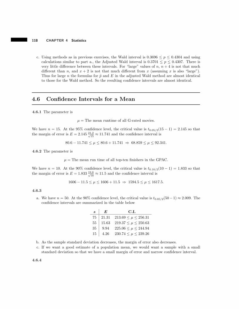
118 CHAPTER 4 Statistics
c. Using methods as in previous exercises, the Wald interval is 0.3696 ! p ! 0.4304 and usingcalculations similar to part a., the Adjusted Wald interval is 0.3701 ! p ! 0.4307. There isvery little di!erence between these intervals. For “large” values of n, n + 4 is not that muchdi!erent than n, and x + 2 is not that much di!erent from x (assuming x is also “large”).Thus for large n the formulas for p and E in the adjusted Wald method are almost identicalto those for the Wald method. So the resulting confidence intervals are almost identical.
4.6 Confidence Intervals for a Mean
4.6.1 The parameter is
µ = The mean runtime of all G-rated movies.
We have n = 15. At the 95% confidence level, the critical value is t0.05/2(15 # 1) = 2.145 so thatthe margin of error is E = 2.145 21.2'
15$ 11.741 and the confidence interval is
80.6# 11.741 ! µ ! 80.6 + 11.741 % 68.859 ! µ ! 92.341.
4.6.2 The parameter is
µ = The mean run time of all top-ten finishers in the GPAC.
We have n = 10. At the 90% confidence level, the critical value is t0.10/2(10 # 1) = 1.833 so thatthe margin of error is E = 1.833 19.8'
10$ 11.5 and the confidence interval is
1606# 11.5 ! µ ! 1606 + 11.5 % 1594.5 ! µ ! 1617.5.
4.6.3
a. We have n = 50. At the 90% confidence level, the critical value is t0.05/2(50# 1) $ 2.009. Theconfidence intervals are summarized in the table below
s E C.I.
75 21.31 213.69 ! µ ! 256.31
55 15.63 219.37 ! µ ! 250.63
35 9.94 225.06 ! µ ! 244.94
15 4.26 230.74 ! µ ! 239.26
b. As the sample standard deviation decreases, the margin of error also decreases.c. If we want a good estimate of a population mean, we would want a sample with a small
standard deviation so that we have a small margin of error and narrow confidence interval.
4.6.4

4.6 Confidence Intervals for a Mean 119
a. Note that since # and z'/2 are fixed values,
limn"$
E = limn"$
z'/2#/n= 0.
b. A larger sample size provides a better estimate of µ since the margin of error is smaller.
4.6.5
a. The parameter is
µ = The mean ratio (overall height)/(navel height of all students at the university.
We have n = 39. At the 99% confidence level, the critical value is t0.01/2(39 # 1) $ 2.704 sothat the margin of error is E = 2.704 0.0474'
39$ 0.0205 and the confidence interval is
1.6494# 0.0205 ! µ ! 1.6494 + 0.0205 % 1.6289 ! µ ! 1.6699.
b. Since this interval contains 1.6494, the results do support the claim.c. These results cannot be used to make any conclusion about the mean ratio of all people in the
world because the sample is not a random sample of people from all over the world.
4.6.6
a. The calculations of the confidence intervals are summarized in the table below.
x s n C.V. E C.I.
BN Sodium 137.79 60.69 74 1.665 11.75 126.04 ! µ ! 149.54
Gen Sodium 158.22 73.3 62 1.671 15.56 142.66 ! µ ! 173.78
BN Sugar 7.77 3.36 74 1.665 0.65 7.12 ! µ ! 8.42
Gen Sugar 7.48 4.49 62 1.671 0.95 6.53 ! µ ! 8.43
b. The intervals for sodium overlap, and so do the intervals for sugar. So there does not appearto be a significant di!erence between the brands.
4.6.7
a. The calculations of the confidence intervals are summarized in the table below.
x s n C.V. E C.I.
Buttered 81.75 32.8976 4 3.182 52.34 29.41 ! µ ! 134.09
Kettle 29.5 19.0875 4 3.182 30.37 #0.87 ! µ ! 59.87
b. Since these intervals overlap, there does not appear to be a significant di!erence between thesetwo population means.

120 CHAPTER 4 Statistics
4.6.8
a. The calculations of the confidence intervals are summarized in the table below.
x s n C.V. E Confidence Interval
Tan 2.511 0.268 30 2.042 0.1 2.41 ! µ ! 2.61
Black 2.621 0.293 30 2.042 0.11 2.51 ! µ ! 2.73
b. Since these intervals overlap, there does not appear to be a significant di!erence between thesetwo population means.
4.6.9 Note that by multiplying by #//n we get
#z'/2 ! Xn # µ
#//n
! z'/2 % #z'/2#/n! Xn # µ ! z'/2
#/n,
then subtracting Xn we get
#Xn # z'/2#/n! #µ ! #Xn + z'/2
#/n,
and multiplying by -1 and reversing the inequalities we get
Xn # z'/2#/n! µ ! Xn + z'/2
#/n.
4.6.10
a. The parameter isµ = The mean height of all supermodels.
We have n = 9. At the 99% confidence level, the critical value is t0.01(9# 1) = 2.896 so thatthe margin of error is E = 2.896 1.4'
9$ 1.35 and the confidence interval is
70.3# 1.35 ! µ < 0 % 68.95 ! µ < 0.
b. The lower confidence interval limit is much greater than 63.5. This suggests that supermodelsare taller than typical women.
4.6.11
a. The parameter is
µ = The mean number of times students call home each week.
We have n = 150. At the 90% confidence level, the critical value is t0.10/2(150# 1) $ 2.351 sothat the margin of error is E = 1.655 1.85'
150$ 0.250. The finite population correction factor is
C =
J650# 150
650# 1$ 0.878,

4.7 Confidence Intervals for a Variance 121
and the confidence interval is
2.3# 0.878(0.25) ! µ ! 2.3 + 0.878(0.25) % 2.081 ! µ ! 2.520.
b. The calculations of the confidence intervals are summarized in the table below. The confidenceinterval for µ1 is narrower than the interval for µ2 this suggests that 10 is probably a slightlybetter estimate of µ1 than µ2.
x s n N C.V. E C C.I.
Pop 1 10 1 100 200 1.66 0.17 0.70888 9.88 ! µ1 ! 10.12
Pop 2 10 1 100 5000000 1.66 0.17 0.99999 9.83 ! µ2 ! 10.17
c. If n is fixed, then limN"$ C = limN"$
JN # n
N # 1= 1. This mean that when the population
size is very large, the correction factor will not significantly change the confidence interval, sothe factor is not necessary.
d. When n = N , C = 0. This means that x is a perfect estimate of µ.
4.6.12 a. We have UCL: y = 62.1 + 3(0.813)//5 = 63.19 and LCL: y = 62.1 # 3(0.813)/
/5 =
61.01 and the center line is y = 62.1. The control chart is shown in Figure 4.12.
61
61
62
62
63
63
64
64
0 1 2 3 4 5 6 7
Sam
ple
Mea
n
Day
Control Chart
Figure 4.12
b. From the control chart, we see that one sample mean is above the UCL, so the process is notin statistical control.
4.7 Confidence Intervals for a Variance
122 CHAPTER 4 Statistics
4.7.1 The parameter is
#2 = The variance of the tensil strength of this type of steel sheet.
We have n = 26. At the 90% confidence level the critical values are
a = (21!0.1/2(26# 1) = 14.61 and b = (2
0.1/2(26# 1) = 37.65.
so that the confidence interval estimate of #2 is
(26# 1)2.41
37.65! #2 ! (26# 1)2.41
14.61% 1.600 ! #2 ! 4.124.
4.7.2 The parameter is
# = The standard deviation of the average velocity of all baseballs hit with a metal bat.
We have n = 26. At the 95% confidence level the critical values are
a = (21!0.05/2(26# 1) = 13.12 and b = (2
0.05/2(26# 1) = 40.65.
so that the confidence interval estimate of #2 is
(26# 1)15.582
40.65! #2 ! (26# 1)15.582
13.12% 149.3 ! #2 ! 462.5
and the confidence interval of # is 12.22 ! # ! 21.51.
4.7.3 The parameter is
# = The standard deviation of the mass of all such candies.
From the data we have n = 17 and s = 0.0509. At the 99% confidence level the critical values are
a = (21!0.01/2(17# 1) = 5.142 and b = (2
0.01/2(17# 1) = 34.27.
so that the confidence interval estimate of #2 is
(17# 1)0.05092
34.27! #2 ! (17# 1)0.05092
5.142% 0.0012 ! #2 ! 0.0081
and the confidence interval of # is 0.0348 ! # ! 0.0898.
4.7.4 The parameter is
#2 = The variance of the lengths of all such bolts.
We have n = 50 and s2 = 0.0023. At the 99% confidence level the critical value for an intervalgiving an upper bound on #2 is
a = (21!0.01(50# 1) $ 29.71

4.7 Confidence Intervals for a Variance 123
so that a one-sided confidence interval estimate of #2 is
0 ! #2 ! (50# 1)0.0023
29.71% 0 ! #2 ! 0.0038
Since this upper limis is less than 0.004, it appears that the manufacturing process meets thespecifications.
4.7.5 The calculations of the confidence intervals are summarized in the table below. Since theseintervals overlap, there does not appear to be a significant di!erence between the variances of thesetwo populations.
s2 n a b C.I.
Male 35.05 18 8.672 27.59 21.60 ! #2M ! 68.71
Female 18.40 8 2.167 14.07 9.15 ! #2F ! 59.44
4.7.6 Suppose a random sample of size n = 10 is taken from a normally distributed populationwith variance #2 = 1.5.
a. As shown in the hint, P!S2 ! 2.446
"$ P (C ! 14.68) where C is (2(9). Examining Table
C.4, we see that (20.1(9) = 14.68. This means that P (C ! 14.68) = 1 # 0.1 = 0.9. Thus
P!S2 ! 2.446
"$ 0.9.
b. By similar arguments as in part a., the event S2 ! 0.83955 corresponds to the event C ! (31#1)(0.83955)/1.5 = 16.791 where C is (2(31#1). Examining Table C.4, we see that (2
0.975(30) =16.79. This means that P (C ! 16.97) = 1# 0.975 = 0.025. Thus P
!S2 ! 0.83955
"$ 0.025.
4.7.7 A confidence interval estimate of #2 is not symmetric around s2, meaning s2 is not halfwaybetween the upper and lower limits. So it is not appropriate to express such a confidence intervalin the form s2 ± E where E is half the width of the confidence interval.
4.7.8 By taking the recriprocal and reversing the inequalities, we get
a ! (n# 1)S2
#2! b % 1
b! #2
(n# 1)S2! 1
a.
Then multiplying by (n# 1)S2 yields
(n# 1)S2
b! #2 ! (n# 1)S2
a.
4.7.9
a. For * = 0.05 and r = 100, z0.5/2 = 1.96,
a $ 1
2
0#1.96 +
/2(100)# 1
12= 73.77, b $ 1
2
01.96 +
/2(100)# 1
12= 129.07
From Table C.4, we find that the exact values of a and b are a = (21!0.5/2(100) = 74.22
and b = (20.05/2(100) = 129.6. The relative errors are |73.77 # 74.22|/74.22 = 0.006 and
|129.07# 129.6|/129.6 = 0.004. These relative errors are extremely small, so the estimates arevery good.

124 CHAPTER 4 Statistics
b. For * = 0.01 and r = 15, z0.01/2 = 2.576,
a $ 1
2
0#2.576 +
/2(15)# 1
12= 3.949, b $ 1
2
02.576 +
/2(15)# 1
12= 31.682
From Table C.4, we find that the exact values of a and b are a = (21!0.01/2(15) = 4.601
and b = (20.01/2(15) = 32.80. The relative errors are |3.949 # 4.601|/4.601 = 0.1417 and
|31.682 # 32.80|/32.80 = 0.0341. These relative errors are much larger than in part a. Thissuggests that the approximation is better for larger values of r.
c. For * = 0.1 and r = 150, z0.1/2 = 1.645,
a $ 1
2
0#1.645 +
/2(150)# 1
12= 122.4, b $ 1
2
01.645 +
/2(150)# 1
12= 179.3
so that the confidence interval estimate of #2 is
(150# 1)2.36
179.3! #2 ! (150# 1)2.36
122.4% 1.961 ! #2 ! 2.873
4.7.10 The calculations are summarized in the table below. We see that s2p = 0.1773/14 = 0.01266
and sp =/0.01266 = 0.11253.
Day s2i ni (ni ! 1) s2i ni ! 1
1 0.0085 5 0.0339 4
2 0.0065 3 0.0131 2
3 0.0235 4 0.0704 3
4 0.0265 2 0.0265 1
5 0.0084 5 0.0335 4
Sum = 0.1773 14
4.8 Confidence Intervals for Di!erences
4.8.1 The parameters are
p1 = the proportion of all plain M&M’s that are blue, and
p2 = the proportion of all peanut M&M’s that are blue.
We have p1 = 62/419 $ 0.148 and p2 = 31/142 $ 0.218 so that p1 # p2 = #0.07 and
p =
J0.148 (1# 0.148)
419+
0.218 (1# 0.218)
142$ 0.0387.
4.8 Confidence Intervals for Di!erences 125
At the 95% confidence level, z0.05/2 = 1.96 so that the margin of error is E = (0.0387)1.96 $ 0.0759and the confidence interval is
#0.07# 0.0759 ! (p1 # p2) ! #0.07 + 0.0759 % #0.1459 ! (p1 # p2) ! 0.0059.
Since this interval contains 0, it appears that the two types of M&M’s contain approximately thesame proportion of blue candies.
4.8.2 The parameters are
p1 = the proportion of all patients given the medication that experience drowsiness, and
p2 = the proportion of all patients given a placebo that experience drowsiness.
We have p1 = 39/1500 = 0.026 and p2 = 19/1550 $ 0.0123 so that p1 # p2 = 0.0137 and
p =
J0.026 (1# 0.026)
1500+
0.0123 (1# 0.0123)
1550$ 0.00497.
At the 95% confidence level, z0.05/2 = 1.96 so that the margin of error is E = (0.00497)1.96 $ 0.00974and the confidence interval is
0.0137# 0.00974 ! (p1 # p2) ! 0.0137 + 0.00974 % 0.00396 ! (p1 # p2) ! 0.0234.
Since the lower limit of this interval is positive, it suggests that the di!erence is positive so thatthose who receive the medicine appear to have a higher proportion of drowsiness. However, theupper limit is 0.0234 suggesting that the di!erence is very small. Because these proportions are solow, drowsiness is not a major concern.
4.8.3 The parameters are defined in the exercise. We have p1 = 228/(228 + 255) = 0.472 andp2 = 503/(503 + 495) $ 0.504 so that p1 # p2 = #0.032 and
p =
J0.472 (1# 0.472)
483+
0.504 (1# 0.504)
998$ 0.0277.
At the 95% confidence level, z0.05/2 = 1.96 so that the margin of error is E = (0.0277)1.96 $ 0.0543and the confidence interval is
#0.032# 0.0543 ! (p1 # p2) ! #0.032 + 0.0543 % #0.0863 ! (p1 # p2) ! 0.0223.
Because this interval contains 0, there does not appear to be much di!erence between morning andevening in terms of the proportion of male users.
4.8.4 The parameters are
p1 = the proportion of all residents living near the location that are in favor, and
p2 = the proportion of all residents living far from the location that are in favor.

126 CHAPTER 4 Statistics
a. We have p1 = 94/125 = 0.752 and p2 = 108/135 = 0.8 so that p1 # p2 = #0.048. Thisdi!erence is small, so there does not appear to be much di!erence.
b. We have
p =
J0.752 (1# 0.752)
125+
0.8 (1# 0.8)
135$ 0.0517.
At the 95% confidence level, z0.05/2 = 1.96 so that the margin of error is E = (0.0517)1.96 $0.101 and the confidence interval is
#0.048# 0.101 ! (p1 # p2) ! #0.048 + 0.101 % #0.149 ! (p1 # p2) ! 0.053.
Because this interval contains 0, there does not appear to be much di!erence between the twogroups of citizens?
c. Let p = the proportion of all residents that are in favor. Combining the samples into one largesample, we get p = (94 + 108)/(125 + 135) = 0.777 and the margin of error is
E = 1.96
J0.777(1# 0.777)
125 + 135$ 0.0506,
and the confidence interval is
0.777# 0.0506 ! p ! 0.777 + 0.0506 % 0.726 ! p ! 0.828.
Since this lower limit is greater than 0.7, it appears that there is at least 70% support.
4.8.5 Since proportions are between 0 and 1, the largest di!erence between two proportions occurswhen one is 1 and the other is 0 which results in a di!erence of absolute value 1. The smallestdi!erence occurs when the two are equal, resulting in a di!erence of 0.
4.8.6 The parameters are
µ1 = the mean volume of all bottles of the first brand, and
µ2 = the mean volume of all bottles of the second brand.
We have n1 = 4, x1 = 510.75, s1 = 1.25, n2 = 4, x2 = 505, s2 = 0.816 , x1 # x2 = 5.75. The pooledstandard deviation is
sp =
J(4# 1)1.252 + (4# 1)0.8162
4 + 4# 2= 1.0555.
At the 95% confidence level, the critical value is t0.05/2(4 + 4 # 2) = 2.447 so that the margin of
error is E = 1.0555(2.447)/
1/4 + 1/4 = 1.826 and the confidence interval is
5.75# 1.826 ! (µ1 # µ2) ! 5.75 + 1.826 % 3.924 ! (µ1 # µ2) ! 7.576.
Since the lower limit is positive, it suggests that there is a significant di!erence between the popu-lation means.

4.8 Confidence Intervals for Di!erences 127
4.8.7 The parameters are
µ1 = the mean average velocity of all balls hit with a metal bat, and
µ2 = the mean average velocity of all balls hit with a wood bat.
We have n1 = 30, x1 = 95.83, s1 = 15.678, n2 = 30, x2 = 81.16, s2 = 10.279 , x1 # x2 = 14.67. Thedegrees of freedom are
r =
=15.6782
30 + 10.2792
30
>2
130!1
!15.6782
30
"2+ 1
30!1
!10.2792
30
"2 = 50.04
so that at the 95% confidence level, the critical value is t0.05/2(50) = 2.009 so that the margin of
error is E = 2.009/
15.6782/30 + 10.2792/30 = 6.877 and the confidence interval is
14.67# 6.877 ! (µ1 # µ2) ! 14.67 + 6.877 % 7.793 ! (µ1 # µ2) ! 21.547.
Since this interval contains 10, the claim that baseballs hit with metal bats travel on average about10 mph fasterappears to be reasonable.
4.8.8 A biologist wants to compare the mean weight of bluegill and the mean weight of catfish ina lake. She captures 23 bluegill and records a mean weight of 1.25 lb with a standard deviation of0.15 lb. She also captures 18 catfish and records a mean of 4.36 lb with a standard deviation of 1.02lb. Assume that the weights of both populations are normally distributed.
a. The sample standard deviations are quite a bit di!erent, so it is not reasonable to assume thepopulation variances are equal.
b. The parameters are
µ1 = the mean weight of all bluegill in the lake, and
µ2 = the mean weight of all catfish in the lake.
We have n1 = 23, x1 = 1.25, s1 = 0.15, n2 = 18, x2 = 4.36, s2 = 1.02 , x1 # x2 = #3.11. Thedegrees of freedom are
r =
=0.152
23 + 1.022
18
>2
123!1
!0.152
23
"2+ 1
18!1
#1.022
18
$2 = 17.58
so that at the 95% confidence level, the critical value is t0.05/2(17) = 2.110 so that the margin
of error is E = 2.110/
0.152/23 + 1.022/18 = 0.511 and the confidence interval is
#3.11# 0.511 ! (µ1 # µ2) ! #3.11 + 0.511 % #3.621 ! (µ1 # µ2) ! #2.599.

128 CHAPTER 4 Statistics
4.8.9 he parameters are
µ1 = the mean GPA of all education majors at the university, and
µ2 = the mean GPA of all non-education majors at the university.
We have n1 = 47, x1 = 3.46, s1 = 0.336, n2 = 53, x2 = 3.38, s2 = 0.449 , x1 # x2 = 0.08.The calculations of the confidence intervals are summarized in the table below. We see that theseconfidence intervals are all very similar. Since they all contain 0, there does not appear to bemuch di!erence between the mean GPA’s of education and non-education majors at this university.However, 0 is near the left end of each interval, so it might be that the education majors have aslightly higher mean GPA.
df C.V. sp E C.I.
Z-interval - 1.960 - 0.1544 #0.0744 ! (µ1 # µ2) ! 0.2344
Equal Var 98 1.984 0.400 0.159 #0.0790 ! (µ1 # µ2) ! 0.2390
Non Equal Var 95.4 1.985 - 0.1564 #0.0764 ! (µ1 # µ2) ! 0.2364
4.8.10 The parameters are
µ1 = the mean run time of all AA batteries of brand A, and
µ2 = the mean run time of all AA batteries of brand B.
a. From the data, we have n1 = 5, x1 = 667, s1 = 38.09, n2 = 5, x2 = 719.4, s2 = 120.8 ,x1 # x2 = #52.4. The degrees of freedom are
r =
=38.092
5 + 120.82
5
>2
15!1
!38.092
5
"2+ 1
5!1
#120.82
5
$2 = 4.79
so that at the 95% confidence level, the critical value is t0.05/2(4) = 2.776 so that the margin
of error is E = 2.776/38.092/5 + 120.82/5 = 157.2 and the confidence interval is
#52.4# 157.2 ! (µ1 # µ2) ! #52.4 + 157.2 % #209.6 ! (µ1 # µ2) ! 104.8.
b. Using software, the critical value is t0.05/2(4.79) = 2.605 yielding E = 147.6 and a confidenceinterval of [#200, 95.2].
c. The di!erence between the intervals is due to the fact that when calculating by hand, werounded r down from 4.79 to 4 to find the critical value whereas the software did not round itdown. Since r is so small, this creates a relatively large di!erence between the critical valuesused in parts a. and b.

4.8 Confidence Intervals for Di!erences 129
4.8.11 The parameters are
µ1 = the mean number of chocolate chips in all cookies of brand A, and
µ2 = the mean number of chocolate chips in all cookies of brand B.
From the data, we have n1 = 20, x1 = 22.2, s1 = 3.222, n2 = 20, x2 = 24.15, s2 = 4.133 ,x1 # x2 = #1.95. The pooled standard deviation is
sp =
J(20# 1)3.2222 + (20# 1)4.1332
20 + 20# 2= 3.706.
At the 90% confidence level, the critical value is t0.1/2(20 + 20 # 2) $ 1.684 so that the margin of
error is E = 3.706(1.684)/
1/20 + 1/20 = 1.974 and the confidence interval is
#1.95# 1.974 ! (µ1 # µ2) ! #1.95 + 1.974 % #3.924 ! (µ1 # µ2) ! 0.024.
Since this interval contains 0, there does not appear to be a significant di!erence between the brands.However, 0 is very near the upper limit, so brand B could contain more.
4.8.12 The parameters are
µ1 = the mean time for all male students, and
µ2 = the mean time for all female students.
From the data, we have n1 = 15, x1 = 28.373, s1 = 11.228, n2 = 15, x2 = 29.953, s2 = 7.448 ,x1 # x2 = #1.58. The pooled standard deviation is
sp =
J(15# 1)11.2282 + (15# 1)7.4482
15 + 15# 2= 9.527.
At the 95% confidence level, the critical value is t0.05/2(15 + 15# 2) = 2.048 so that the margin of
error is E = 9.527(2.048)/
1/15 + 1/15 = 7.125 and the confidence interval is
#1.58# 7.125 ! (µ1 # µ2) ! #1.58 + 7.125 % #8.705 ! (µ1 # µ2) ! 5.545.
Since this interval contains 0, there does not appear to be a significant di!erence between theabilities of males and females to estimate when 30 seconds has passed.
4.8.13 The parameter is
µd = The mean di!erence (first error - second error) of all students.
The values of the di!erences in the sample are shown in the table below. We have n = 18, x = 0.3611,and s = 4.92. At the 95% confidence level, the critical value is t0.05/2(18 # 1) = 2.110 so that themargin of error is E = 2.110 4.92'
18= 2.447 and the confidence interval is
0.3611# 2.447 ! µd ! 0.3611 + 2.447 % #2.086 ! µd ! 2.808.
Since the confidence interval contains 0, the second error does not appear to be smaller than thefirst, on average.
130 CHAPTER 4 Statistics
First Error 2 2 9 4 6 3 15 2 1.5 2 0 5 1 2 2 5 10 4
Second Error 7 1 2 2 2 9 5 3 10 7 5 2 3 2 0 1 5 3
Di!erence -5 1 7 2 4 -6 10 -1 -8.5 -5 -5 3 -2 0 2 4 5 1
4.8.14 The parameter is
µd = The mean di!erence (before - after) of all athletes who took this training program.
The values of the di!erences in the sample are shown in the table below. We have n = 8, x = 1.613,and s = 1.131. At the 95% confidence level, the critical value is t0.05/2(8 # 1) = 2.365 so that themargin of error is E = 2.365 1.131'
8= 0.946 and the confidence interval is
1.613# 0.946 ! µd ! 1.613 + 0.946 % 0.667 ! µd ! 2.559.
Since the lower limit is positive, it appears that the training program does have a significant e!ecton track times.
Before 53.8 54.2 52.9 53 55.1 58.2 56.7 52
After 52.7 53.8 51.1 52.7 54.2 55.4 53.3 49.8
Di!erence 1.1 0.4 1.8 0.3 0.9 2.8 3.4 2.2
4.8.15 The parameter is
µd = The mean di!erence (with - withou) of all athletes.
The values of the di!erences in the sample are shown in the table below. We have n = 10, x = 0.6,and s = 1.075. At the 95% confidence level, the critical value is t0.05/2(10# 1) = 2.262 so that themargin of error is E = 2.262 1.075'
10= 0.769 and the confidence interval is
0.6# 0.769 ! µd ! 0.6 + 0.769 % #0.169 ! µd ! 1.369.
Since this interval contains 0, it does not appear that shoes significantly a!ect vertical jump height.
With 15.5 18.5 22.5 17.5 16.5 17.5 20.5 15.5 19.5 18.5
Without 15.5 17.5 22.5 15.5 15.5 18.5 21.5 14.5 17.5 17.5
Di!erence 0 1 0 2 1 -1 -1 1 2 1
4.8.16
a. We havd n1 = n2 = 10 so that by this alternative formula, r = 9 so that the critical valueis t0.05/2(9) = 2.262 and the margin of error is E = 2.262
/6.52/10 + 4.52/10 = 5.655. This
yields the confidence interval #4.355 ! µ1 # µ2 ! 6.955.b. In part a., we have a much smaller degrees of freedom and a wider confidence interval than in
the example.

4.8 Confidence Intervals for Di!erences 131
c. Without loss of generality, we assume that n1 " n2. To simplify notation, let a = s21/n21 and
b = s22/n22 so that
r =(a+ b)2
a2
n1 # 1+
b2
n2 # 1
=(n2 # 1) (a+ b)2#n2 # 1
n1 # 1
$a2 + b2
by multiplying byn2 # 1
n2 # 1
" (n2 # 1) (a+ b)2
a2 + b2since
n2 # 1
n1 # 1! 1
"(n2 # 1)
!a2 + b2
"
a2 + b2since (a+ b)2 > a2 + b2
= n2 # 1
Thus r " n2 # 1. Since n2 # 1 ! n1 # 1, r is greater than the smaller of n1 # 1 and n2 # 1.d. Using a smaller value of r yields a larger critical value and a wider confidence interval. This
means that more than 100(1 # *)% of confidence intervals would contain the true value of(µ1 # µ2).
4.8.17
a. If r increases, the critical value gets smaller.b. The confidence interval would be narrower.c. Rounding down gives a wider confidence interval which mean we are more confident that the
interval contains the true value of the di!erence. It is better to be more confident than lessconfident.
4.8.18
a. The parameters are defined in the exercise. We have p1 = 19/175 = 0.109 and p2 = 6/154 =0.0390 so that p1 # p2 = 0.07. We have
p =
J0.109 (1# 0.109)
175+
0.0390 (1# 0.0390)
154$ 0.0283.
At the 95% confidence level, z0.05 = 1.645 so that the margin of error is E = 0.0283(1.645) =0.0465 and the confidence interval is
0.07# 0.0465 ! (p1 # p2) ! 1 % 0.0235 ! (p1 # p2) ! 1.
b. Since this lower limit is greater than 0.02, it appears that the percentage of defects has beenreduced by at least two percentage points.

132 CHAPTER 4 Statistics
4.8.19 The parameters are defined in the exercise. We have n1 = 27 x1 = 600, s1 = 80, n2 = 25,x2 = 533, s2 = 118 , x1 # x2 = 67. The pooled standard deviation is
sp =
J(27# 1)802 + (25# 1)1182
27 + 25# 2= 100.06.
At the 95% confidence level, the critical value is t0.05(27 + 25 # 2) = 1.676 so that the margin oferror is E = 100.06(1.676)
/1/27 + 1/25 = 46.55 and the confidence interval is
67# 46.55 ! (µ1 # µ2) < 0 % 20.45 ! (µ1 # µ2) < 0.
Since this lower limit is greater than 20, it appears that the score increase by at least 20 points, sothe data do support the claim.
4.9 Sample Size
4.9.1 Starting with E = z'/2/p (1# p) /n, we square both sides, multiply by n, and divide by E
to get n = z2'/2p (1# p) /E2.
4.9.2 We have p = 0.75, E = 0.015, and z0.10/2 = 1.645 so that
n =1.6452(0.75) (1# 0.75)
0.0152= 2255.02.
Thus they must survey at least 2256 students.
4.9.3 We have p = 0.5, E = 0.04, and z0.05/2 = 1.96 so that
n =1.962(0.5) (1# 0.5)
0.042= 600.25.
Thus they must survey at least 601 voters.
4.9.4 Consider the function f(x) = x(1 # x) = x # x2 over the interval 0 ! x ! 1. Thenf %(x) = 1 # 2x. Setting f % equal to 0 yields x = 1/2. Then f(0) = f(1) = 0 and f(1/2) = 1/4.Thus the maximum value of f is 1/4 so that x(1# x) ! 1/4 for all x between 0 and 1. Changing xto p, we get p (1# p) ! 1/4 for all values of p between 0 and 1.
4.9.5 We have E = 0.25 and z0.1/2 = 1.645. Taking 1.3 as an estimate of # we get a necessarysample size of
n =1.6452(1.32)
0.252= 73.2
so that we need a total of 74. Since we have already sampled 15, we need an additional 59 fish.
4.9.6
4.9 Sample Size 133
a. We have E = 0.02 and z0.05/2 = 1.96. Taking 0.2 as an estimate of # we get a necessarysample size of
n =1.962(0.22)
0.022= 384.2
so that we need to sample at least 385 batteries.
b. The parameter isµ = The mean life-span of the new batteries.
We have n = 400. At the 95% confidence level, the critical value is t0.05/2(400# 1) $ 1.966 sothat the margin of error is E = 1.966 0.18'
400$ 0.01769 and the confidence interval is
9.05# 0.01769 ! µ ! 9.05 + 0.01769 % 9.032 ! µ ! 9.068.
Since this lower limit is greater than 8.9, it appears that the mean life span has increased.
4.9.7 A student would like to estimate the mean GPA of all education majors at a large university.She believes that most of the GPA’s will lie between 2.5 and 3.8.
a. According to equation (4.10), # $ (3.8# 2.5)/4 = 0.325.
b. We have E = 0.1 and z0.01/2 = 2.576 so that
n =2.5762(0.3252)
0.12= 70.04.
Thus she needs to survey at least 71 students.
4.9.8 We have E = 0.1# and z0.1/2 = 1.645 so that
n =1.6452#2
(0.1#)2= 270.6. (4.1)
Thus the sample size needs to be at least 271.
4.9.9 The population of professors is probably more homogeneous than the general population.This means that the variance of the population of professors is probably less than 152. This meansthat the sample size calculated in Example 4.9.3 is probably larger than needed.
4.9.10
a. Using E = 0.02 and p = 0.5, we get necessary sample sizes of 80%: 1027, 90%: 1692, 95%:2401, and 99%: 4148.
b. As the confidence level increases, the necessary sample size also increases.
c. Using z0.05/2 = 1.96 and p = 0.5, we get necessary sample sizes of E = 0.015: 4269, E = 0.01:9604, E = 0.005: 38416
d. As the margin of error decreases, the necessary sample size increases.
4.9.11

134 CHAPTER 4 Statistics
a. We have p = 0.5, E = 0.01, and z0.01/2 = 2.576 so that
n =2.5762(0.5) (1# 0.5)
0.012= 16590.
b. They can lower their confidence level or increase the desired margin of error.
4.9.12
a. With E = 0.1 at the 95% confidence level, the sample size is n = 1.962p (1# p) /0.12 =384.16p (1# p). Now consider the function f(x) = 38.016x(1# x) = 384.16
!x# x2
"over the
interval 0 ! x ! 1. Then f %(x) = 384.16(1# 2x). Setting f % equal to 0 yields x = 1/2. Thenf(0) = f(1) = 0 and f(1/2) = 96.04. Thus f is maximized at x = 1/2. This means that thelargest sample size occurs when p = 0.5.
b. Using the same arguments as in part a., we get that the largest sample size occurs whenp = 0.5.
c. Since a larger random sample will always give a smaller margin of error, when in doubt, wewould prefer to use a larger sample size than a smaller one. Using p = 0.5 gives us the samplesize at least as large as we need to achieve the desired margin of error.
4.9.13 We need to find the smallest value of n such that (n # 1)!1a # 1
b
"< 1.52 where a =
(20.975(n# 1) and b = (2
0.025(n# 1). The calculations in the following table show that the necessarysample size is n = 21.
n a = "20.975(n! 1) b = "2
0.025(n! 1) (n! 1)!1a! 1
b
"
18 7.5642 30.1910 1.6844
19 8.2307 31.5264 1.6160
20 8.9065 32.8523 1.5549
21 9.5908 34.1696 1.5000
4.9.14
a. We have N = 1000, n = 100, p = 65/100 = 0.65 and z0.1/2 = 1.645 so that the margin of erroris
E = 1.645
K0.65 (1# 0.65)
100
#1000# 100
1000# 1
$= 0.0745 (4.2)
and the confidence interval is
0.65# 0.0745 ! p ! 0.65 + 0.0745 % 0.5755 ! p ! 0.7245.
b. Using N = 800, E = 0.05, and p = 0.5, we get
k =1.6452(0.5) (1# 0.5)
0.052= 270.6 % n =
270.6
1 + 270.6!1800
= 203.

4.9 Sample Size 135
c. Note that k does not depend on N , so k = 270.6 for every value of N . The values of n aresummarized in the table below. We see that as N gets larger, n gets closer to k
N 2,000 5,000 10,000 100,000 1,000,000
n 239 257 264 270 271
d. The sample size given by formula (4.7) is the same as k. The sample size for a small populationgiven by formula (4.12) is less than k because the denominator is greater than 1. Thus usingformula (4.7) for a small population gives us an over-estimate of the necessary sample size.
e. This “finite population correction” is a rational expression in N where the degree of thenumerator equals the degree of the denominator. Thus the limit as N 1 0 equals the ratio ofthe leading coe"cients, 1/1 = 1. This means that as the population gets larger, the correctionterm is not needed.
4.9.15
a. We begin by dividing both sides by z'/2, squaring both sides, and adding the fractions on theright-hand side to get #
E
z'/2
$2
=p1 (1# p1) + p2 (1# p2)
n.
Taking the reciprocal of both sides and multiplying by [p1 (1# p1) + p2 (1# p2)] yields
n ==z'/2
E
>2[p1 (1# p1) + p2 (1# p2)] .
b. Using E = 0.04, p1 = p2 = 0.5, and z0.05/2 = 1.96, we get
n =
#1.96
0.04
$2
[0.5 (1# 0.5) + 0.5 (1# 0.5)] = 1200.5
so that the necessary sample size is 1201.
4.9.16
a. We begin by dividing both sides by z'/2, squaring both sides, and adding the fractions on theright-hand side to get #
E
z'/2
$2
=#21 + #2
2
n
Taking the reciprocal of both sides and multiplying by!#21 + #2
2
"yields
n ==z'/2
E
>2 !#21 + #2
2
".

136 CHAPTER 4 Statistics
b. Using E = 0.75, #21 = 1.5, #2
2 = 5.6, and z0.01/2 = 2.576, we get
n =
#2.576
0.75
$2
(1.5 + 5.6) = 83.8
so that the necessary sample size is 84.
4.10 Assessing Normality
4.10.1 Replacing yk with y and xk with x, we see that these points satisfy the relation y =(x# x) /s = (1/s)x# x/s. But s and x/s are constant for a given set of data, so the relation is ofthe form y = mx + b where m and b are constants. Graphically, this relationship forms a straightline.
4.10.2 The calculations and quantile plot are shown in Figure 4.13. The dots do not lie very closeto the straight line, so it is not reasonable to assume the population is normally distributed.
k x Percentile z-score
1 52.3 0.0833 -1.3830
2 56.8 0.1667 -0.9674
3 57.8 0.2500 -0.6745
4 60.7 0.3333 -0.4307
5 70.9 0.4167 -0.2104
6 89.9 0.5000 0.0000
7 91.7 0.5833 0.2104
8 92.6 0.6667 0.4307
9 92.7 0.7500 0.6745
10 92.8 0.8333 0.9674
11 93.9 0.9167 1.3830
x = 77.46
s = 17.59
-2
-2
-1
-1
0
1
1
2
2
50 60 70 80 90 100
z-sc
ore
Exam Score
Quantile Plot
Figure 4.13
4.10.3 The calculations and quantile plot are shown in Figure 4.14. The dots exhibit a pattern, soit is not reasonable to assume the population is normally distributed.

4.10 Assessing Normality 137
k x Percentile z-score
1 0 0.0526 -1.6199
2 1 0.1053 -1.2521
3 1.5 0.1579 -1.0031
4 2 0.2105 -0.8046
5 2 0.2632 -0.6336
6 2 0.3158 -0.4795
7 2 0.3684 -0.3360
8 2 0.4211 -0.1992
9 2 0.4737 -0.0660
10 3 0.5263 0.0660
11 4 0.5789 0.1992
12 4 0.6316 0.3360
13 5 0.6842 0.4795
14 5 0.7368 0.6336
15 6 0.7895 0.8046
16 9 0.8421 1.0031
17 10 0.8947 1.2521
18 15 0.9474 1.6199
x = 4.194
s = 3.785
-2-2-1-101122334
-1 1 3 5 7 9 11 13 15
z-sc
ore
Error
Quantile Plot
Figure 4.14
-2
-2
-1
-1
0
1
1
2
2
3
0.72 0.74 0.76 0.78 0.8 0.82 0.84 0.86 0.88
z-sc
ore
Proportion of Butterfat
Quantile Plot
Figure 4.15

138 CHAPTER 4 Statistics
4.10.4 The quantile plot is shown in Figure 4.15. The dots lie close to the straight line and do notexhibit any pattern, so it is reasonable to assume the population is normally distributed.
4.10.5 The quantile plots are shown in Figure 4.16. The normality of the name brand and genericB times are somewhat questionable. However, the dots do not lie that far from the line to rejectnormality. So it appears to be reasonable to assume that all three populations are normal.
-2
-2
-1
-1
0
1
1
2
800 850 900 950 1000 1050 1100 1150 1200
z-sc
ore
Minutes
Quantile Plot of Name Brand
-2
-1
-1
0
1
1
2
2
600 620 640 660 680 700 720 740z-
scor
e
Minutes
Quantile Plot of Generic A
-2
-1
-1
0
1
1
2
2
550 650 750 850 950
z-sc
ore
Minutes
Quantile Plot of Generic B
Figure 4.16
4.10.6 The quantile plots are shown in Figure 4.17. It appears reasonable to assume that brand Bis normal. For brand A, the numerous data values of 23 and 24 cause us to question the assumptionof normality, but the assumption does not appear to be too unreasonable.
4.10.7 The quantile plots are shown in Figure 4.18. The assumptions of normality appear reasonablefor both populations.
4.10.8 The quantile plot is shown in Figure 4.19. The assumption of normality appears to bereasonable.
4.10.9 The calculations and probability plot are shown in Figure 4.20. We see that the dots do lienear the straight line. Thus the population appears to have an exponential distribution.

4.10 Assessing Normality 139
-2
-2
-1
-1
0
1
1
2
2
15 17 19 21 23 25 27 29
z-sc
ore
Number of Chocolate Chips
Quantile Plot of Brand A
-2
-2
-1
-1
0
1
1
2
2
15 17 19 21 23 25 27 29 31
z-sc
ore
Number of Chocolate Chips
Quantile Plot of Brand B
Figure 4.17
-2-2
-1-1
01
1
22
3
15 20 25 30 35 40 45 50 55
z-sc
ore
Times
Quantile Plot of Males
-2
-2
-1
-1
0
1
1
2
2
15 20 25 30 35 40 45
z-sc
ore
Times
Quantile Plot of Females
Figure 4.18
-2
-2
-1
-1
0
1
1
2
2
3
-10 -5 0 5 10
z-sc
ore
Errors
Quantile Plot
Figure 4.19

140 CHAPTER 4 Statistics
k x pk #k
1 0.1 0.0625 0.1291
2 0.2 0.1250 0.2671
3 0.3 0.1875 0.4153
4 0.5 0.2500 0.5754
5 0.7 0.3125 0.7494
6 1.2 0.3750 0.9400
7 1.7 0.4375 1.1507
8 1.7 0.5000 1.3863
9 2.1 0.5625 1.6534
10 2.2 0.6250 1.9617
11 2.5 0.6875 2.3263
12 2.9 0.7500 2.7726
13 3.4 0.8125 3.3480
14 4.5 0.8750 4.1589
15 5.5 0.9375 5.5452
0
1
2
3
4
5
6
7
0 1 2 3 4 5 6
π
x
Probability Plot
Figure 4.20
Chapter 5
Hypothesis Testing
5.1 Introduction
5.1.1 The claim is made about the population of all kindergarten students. In order to prove herclaim, she would need to weigh every kindergarten student. She does not do this. She weighs onlya sample of students. The sample mean of x = 48.6 is only an estimate of the population mean sheis making a claim about.
5.1.2 This is the correct conclusion because she is making a claim about only those candies inthe particular bag. She weighs every candy so the mean of 0.048 is the exact value of what she ismaking a claim about.
5.1.3 A sample proportion less than 0.5 cannot support a claim that a population proportion isgreater than 0.5. So no hypothesis test is needed.
5.1.4
a. p = proportion of all citizens of the United States that own a homeb. p= proportion of all introduction to statistics students that spend more than one hour studying
for their tests.c. µ = mean IQ score of all professorsd. # = standard deviation of all scores on the SATe. µ = mean weight of all 12 oz packages of shredded cheddar cheese
5.1.5
a. z0.10 = 1.282, (#0, #1.282], P-value = P (Z ! #1.24) = 0.1075, do not reject H0
b. z0.05/2 = 1.960, (#0, #1.960] ( [1.960, 0), P-value = 2 · P (Z > 2.67) = 0.0076, reject H0
141

142 CHAPTER 5 Hypothesis Testing
c. z0.01 = 2.326, [2.326, 0), P-value = P (Z > 0.87) = 0.1922, do not reject H0
5.1.6
a. There is su"cient evidence to reject the claim.b. The data do not support the claim.c. The data support the claim.
5.1.7 The claim is that p < 0.75 so that the hypotheses are
H0 : p = 0.75, H1 : p < 0.75.
P-value = P (Z ! #2.77) = 0.0028 < 0.10 so we reject H0 and conclude that the data support theclaim. Supporting the claim that p < 0.75 does not contradict the original conclusion of rejectingthe claim that p = 0.75. There would be a contradiction if we supported both claims.
5.1.8
a. Since the numerator is p# p0, if z < 0, then p0 is larger.b. In this case they are equal.c. The P-value in a left-tail test is P (Z ! z). If this probability is greater than 0.5, then z must
be positive. By the reasoning in part a., this means that p is larger.d. First assume the test statistic z is negative. Then P-value = 2 · P (Z ! z) > 0.5. This means
that P (Z ! z) > 0.25. By examining the z-score table, we see this is true for approximatelyz > #0.675. By similar arguments, if z is positive, then z < 0.675. Therefore, #0.675 < z <0.675.
e. No. A P-value is a probability. Probabilities must be between 0 and 1.f. The P-value was probably given in scientific notation and the student missed the power of 10.
Rounded to 4 decimal places, the P-value is probably 0.0000.
5.1.9
a. The respective values of z are 0.283, -0.566, 2.828, -3.677, and 0 .b. If p > p0, then z > 0. If p < p0, then z < 0. If p = p0, then z = 0. If p is further in value from
p0, then z gets larger in absolute value.
5.2 Testing Claims about a proportion
5.2.1 Let p = the proportion of all users of the allergy medicine that experience drowsiness. Theclaim is that p < 0.10 and the hypothesess are
H0 : p = 0.10, H1 : p < 0.10.
5.2 Testing Claims about a proportion 143
We have n = 75, p = 3/75 = 0.04, and z = 0.4!0.5/0.5(1!0.5)/75
= #1.73. At the 0.05 significance
level, the critical value is z0.05 = 1.645 and the critical region is (#0, #1.645]. Also, P-value= P (Z ! #1.73) = 0.0418. At the 0.05 significance level, we reject H0 and conclude that the datasupport the claim. At the 0.01 significance level, the critical region is (#0, #2.326] so that wewould not reject H0. The di!erent significance level yields a di!erent conclusion.
5.2.2
a. Let p = the proportion of all consumers who prefer the Better Bread company’s classic whitebread over their main competitor’s. The claim is that p > 0.75 and the hypothesess are
H0 : p = 0.75, H1 : p > 0.75.
We have n = 150, p = 115/150 = 0.767, and z = 0.767!0.75/0.75(1!0.75)/150
= 0.48. At the 0.05
significance level, the critical value is z0.05 = 1.645 and the critical region is [1.645, 0). Also,P-value = P (Z > 0.48) = 0.3156. At the 0.05 significance level, we do not reject H0 andconclude that the data do not support the claim.
b. If p0 = 0.70, we have z = 1.78 and P-value = 0.0375. So we reject H0 and conclude that thedata support the claim.
c. Our hypothesis tests support the second claim, not the first. So it would be more accurate toclaim “More than 70% prefer our bread.”
5.2.3 Let p = the proportion of all voters in the 2006 Nebraska governor’s election that were age65 and oler. The claim is that p < 0.25 and the hypothesess are
H0 : p = 0.25, H1 : p < 0.25.
We have n = 1008, p = 0.24, and z = 0.24!0.25/0.25(1!0.25)/1008
= #0.73. At the 0.05 significance level,
the critical value is z0.05 = 1.645 and the critical region is [#0, #1.645]. Also, P-value = P (Z <#0.73) = 0.2327. We do not reject H0 and conclude that the data do not support the claim. Thusit would not be appropriate to include this statement in the article.
5.2.4 Let p = the proportion of all cereals that are high-sugar. The claim is that p > 0.5 and thehypothesess are
H0 : p = 0.5, H1 : p > 0.5.
We have n = 120, p = 70/120 = 0.583, and z = 0.583!0.5/0.5(1!0.5)/120
= 1.82. At the 0.05 significance
level, the critical value is z0.05 = 1.645 and the critical region is [1.645, 0). Also, P-value = P (Z >1.82) = 0.0344. We reject H0 and conclude that the data support the claim.
5.2.5 Let p = the proportion of all ghost crabs with a larger left claw. The claim is that p > 0.5and the hypothesess are
144 CHAPTER 5 Hypothesis Testing
H0 : p = 0.5, H1 : p > 0.5.
We have n = 72, p = 41/72 = 0.569, and z = 0.569!0.5/0.5(1!0.5)/72
= 1.18. At the 0.05 significance level,
the critical value is z0.05 = 1.645 and the critical region is [1.645, 0). Also, P-value = P (Z >1.18) = 0.119. We do not reject H0 and conclude that the data do not support the claim. Basedon this conclusion, it does not appear that ghost crabs have a genetic disposition to having a largerleft claw.
5.2.6 Let p = the proportion of all pool balls that are pocketed behind the rack. The claim is thatp > 0.5 and the hypothesess are
H0 : p = 0.5, H1 : p > 0.5.
We have n = 130, p = 75/130 = 0.577, and z = 0.577!0.5/0.5(1!0.5)/130
= 1.75. At the 0.05 significance
level, the critical value is z0.05 = 1.645 and the critical region is [1.645, 0). Also, P-value = P (Z >1.75) = 0.0401. We reject H0 and conclude that the data support the claim.
5.2.7 Let p = the proportion of all fired FBS coaches that had a winning percentage less than0.500. The claim is that p > 0.5 and the hypothesess are
H0 : p = 0.5, H1 : p > 0.5.
We have n = 39, p = 30/39 = 0.770, and z = 0.770!0.5/0.5(1!0.5)/39
= 3.36. At the 0.05 significance level,
the critical value is z0.05 = 1.645 and the critical region is [1.645, 0). Also, P-value = P (Z >3.36) = 0.0004. We reject H0 and conclude that the data support the claim. This result suggeststhat most coaches who get fired have a losing record. It does not establish a cause-and-e!ectrelationship.
5.2.8 Let p = the proportion of all spins of a penny that land tails up. The claim is that p = 0.5and the hypothesess are
H0 : p = 0.5, H1 : p += 0.5.
We have n = 500, p = 296/500 = 0.592, and z = 0.592!0.5/0.5(1!0.5)/500
= 4.11. At the 0.05 significance
level, the critical value is z0.05/2 = 1.96 and the critical region is (#0, #1.96] ( [1.96, 0). Also,P-value = 2 · P (Z > 4.11) = 0.0000. We reject H0 and conclude that the data support the claim.This suggests that spinning a penny does not produce the same results as flipping a penny.
5.2.9 Let p = the proportion of all ice-cream eating students who choose vanilla over chocolate ortwist. The claim is that p > 0.5 and the hypothesess are
H0 : p = 0.5, H1 : p > 0.5.
5.2 Testing Claims about a proportion 145
We have n = 56, p = 35/56 = 0.625, and z = 0.625!0.5/0.5(1!0.5)/56
= 1.87. At the 0.05 significance level,
the critical value is z0.05 = 1.645 and the critical region is [1.645, 0). Also, P-value = P (Z >1.87) = 0.0307. We reject H0 and conclude that the data support the claim.
5.2.10 Let p = the proportion of all babies born that are girls. The claim is that p = 0.5 and thehypothesess are
H0 : p = 0.5, H1 : p += 0.5.
We have n = 3465, p = 1712/3465 = 0.494, and z = 0.494!0.5/0.5(1!0.5)/3465
= #0.70. At the 0.05
significance level, the critical value is z0.05/2 = 1.96 and the critical region is (#0, #1.96]([1.96, 0).Also, P-value = 2 · P (Z ! #0.70) = 0.4840. We do not reject H0 and conclude that there is notsu"cient evidence to reject the claim. Thus our assumption that P (girl) = P (boy) = 0.5 appearsto be reasonable.
5.2.11 Let p = the proportion of red and blue candies that are red. The claim is that p > 0.5 andthe hypothesess are
H0 : p = 0.5, H1 : p > 0.5.
We have n = 120, p = 65/120 = 0.542, and z = 0.542!0.5/0.5(1!0.5)/120
= 0.91. At the 0.05 significance
level, the critical value is z0.05 = 1.645 and the critical region is [1.645, 0). Also, P-value = P (Z >0.91) = 0.1814. We do not reject H0 and conclude that the data do not support the claim.
5.2.12
a. Let p = the proportion of all car crashes that occur within 5 miles of the home of the driver.The claim is that p < 0.25 and the hypothesess are
H0 : p = 0.25, H1 : p < 0.25.
We have n = 120, p = 62/120 = 0.517, and z = 0.517!0.25/0.25(1!0.25)/120
= 6.75. At the 0.05
significance level, the critical value is z0.05 = 1.645 and the critical region is (#0, #1.645].Also, P-value = P (Z < 6.75) = 1. We do not reject H0 and conclude that the data do notsupport the claim. The claim it not at all reasonable.
b. Since the sample proportion is greater than 0.25, there is no way the data could support theclaim.
5.2.13
a. The test statistics are z = 0.89, 1.26, 1.55, 1.78, 2, respectively. The corresponding P-valuesare 0.1867, 0.1038, 0.0606, 0.0375, 0.0228. For the first 3 values of n, we do not reject H0
while we do reject H0 for the last 2 values.b. limn"$ z = 0, limn"$(P-value) = 0

146 CHAPTER 5 Hypothesis Testing
c. Larger values of n give smaller P-values, so we would be more confident in rejecting H0 andsupporting the claim.for larger values of n.
5.2.14
a. Using software, P (X ! 37) = 0.028732. This exact P-value is slightly higher than the approx-imate value found in the example, but it does not change the conclusion.
b. Using software, if X is b(0.3, 350), then P (X " 120) = 0.04666. To find the approximate P-value, p = 120/350 = 0.343 so that z = 0.343!0.3/
0.3(1!0.3)/350= 1.75 and P-value = P (Z > 1.75) =
0.0401. The exact P-value is slightly higher than the approximate, but not enough to changethe conclusion.
c. Using software, if X is b(100, 0.3), then p1 = P (X ! 24) = 0.11357. Values of P (X " x)for di!erent values of x are shown in the table below. We see that the closest probability lessthan 0.11357 is 0.07988. Thus x2 = 37 and the exact P-value is 0.11357 + 0.07988 = 0.19345.
x 35 36 37 38 39
P (X " x) 0.16286 0.11608 0.07988 0.05305 0.03398
5.2.15 The polling results example is a two-tail test, so we calculate a two-sided confidence interval.We have n = 350, p = 0.686, and the critical value is z0.10/2 = 1.645 so that the margin of error is
E = 1.645
J0.686 (1# 0.686)
350= 0.041
and the confidence interval is 0.686 # 0.041 ! p ! 0.686 + 0.041 % 0.645 ! p ! 0.727. Thisconfidence interval does not contain 0.75, so we reject H0 which is the same conclusion as in theexample.
The M&M example is a left-tail test, so we calculate a one-sided confidence interval that gives anupper bound on p. We have n = 195, p = 0.190, and the critical value is z0.05 = 1.645 so that themargin of error is
E = 1.645
J0.190 (1# 0.190)
195= 0.046
and the confidence interval is 0 ! p ! 0.190 + 0.046 % 0 ! p ! 0.236. This confidence intervaldoes not contain 0.25 so we reject H0 which is the same conclusion as in the example.
5.2.16
a. We have n = 100, p0 = 0.45, and the critical z-value is z0.05 = 1.645. The critical value of p is
p = 1.645/0.45 (1# 0.45) /100 + 0.45 = 0.5318.
We would reject H0 if p > 0.5318. Now, P is approximately N(0.6, 0.6(1 # 0.6)/100) =
N(0.6, 0.0024), so the power of the test is P=P > 0.5318
>$ P (Z > #1.39) = 0.9177. This
is a higher power than when p0 = 0.5 and suggests that as p0 gets further in value from p, thepower increases.

5.3 Testing Claims about a Mean 147
b. With p0 = 0.5 and n = 500, the critical value of p is
p = 1.645/0.5 (1# 0.5) /500 + 0.5 = 0.5368.
Now, P is approximately N(0.6, 0.6(1# 0.6)/500) = N(0.6, 0.00048), so the power of the test
is P=P > 0.5368
>$ P (Z > #2.88) = 0.9980. This is a higher power than when p0 = 0.5 and
n = 100 and suggests that as n gets larger, the power increases.
c. With p0 = 0.5, n = 100, and * = 0.2, the critical z-value is z0.2 = 0.842. The critical value ofp is
p = 0.842/0.5 (1# 0.5) /100 + 0.5 = 0.5421.
Now, P has the same distribution as in part a., so the power of the test is P=P > 0.421
>$
P (Z > #1.18) = 0.8810. This is a higher power than when /alpha = 0.05 as in the exampleand suggests that as * gets larger, the power increases.
5.2.17 We have n = 200, p0 = 0.30, p = 0.20, and the critical z-value is #z0.01 = #2.326. Thecritical value of p is
p = #2.326/
0.3 (1# 0.3) /200 + 0.3 = 0.2246.
We would rejectH0 if p < 0.2246. Now, P is approximatelyN(0.2, 0.2(1#0.2)/200) = N(0.2, 0.0008),
so the power of the test is P=P < 0.2246
>$ P (Z < 0.87) = 0.8078.
5.2.18 We have n = 150, p0 = 0.75, p = 0.70, and the critical z-value is #z0.05 = #1.645. Thecritical value of p is
p = #1.645/0.75 (1# 0.75) /150 + 0.75 = 0.6918.
We would rejectH0 if p < 0.6918. Now, P is approximatelyN(0.7, 0.7(1#0.7)/150) = N(0.7, 0.0014),
so the power of the test is P=P < 0.6918
>$ P (Z < #0.22) = 0.4129. This is a higher power than
in the example, so this test would be more likely to detect the change.
5.3 Testing Claims about a Mean
5.3.1
a. Between 0.025 and 0.05
b. Between 0.05 and 0.10
c. Greater than 0.10
5.3.2 The claim is about the mean weight of all 12 oz packages of shredded cheddar, not just the36 in the sample. The sample mean is an estimate of the population mean. These two means arenot the same thing.

148 CHAPTER 5 Hypothesis Testing
5.3.3 Let µ = the mean reading at the freezing point of water of all thermometers from the assemblyline. The claim is µ = 0 and the hypotheses are
H0 : µ = 0, H1 : µ += 0.
We have # = 1, n = 75, and x = 0.12 so the test statistic is z = 0.12!01/
'75
= 1.04. At the 0.05
significance level, the critical value is z0.05/2 = 1.96 and the critical region is (#0, #1.96]([1.96, 0).Also, P-value = 2 · P (Z > 1.04) = 0.2984. We do not reject H0 and conclude that there is notsu"cient evidence to reject the claim. Thus it appears that these thermometers do give a readingof 0 (C, on average.
5.3.4 Let µ = the mean square footage of all homes within a five-mile radius of this lake. Theclaim is µ > 1931 and the hypotheses are
H0 : µ = 1931, H1 : µ > 1931.
We have s = 856.8, n = 30, and x = 2421.7 so the test statistic is t = 2421.7!1931856.8/
'30
= 3.137. At the
0.05 significance level, the critical value is t0.05(29) = 1.699 and the critical region is [1.699, 0).Using software, P-value = P (T > 3.137) = 0.0019. We reject H0 and conclude that the data supportthe claim. Thus it appears that homes around this lake tend to be larger than a typical home.
5.3.5 Let µ = the mean weight loss of all people on this program. The claim is µ < 0 and thehypotheses are
H0 : µ = 0, H1 : µ < 0.
We have s = 10.3, n = 50, and x = #7.7 so the test statistic is z = !7.7!010.3/
'50
= #5.29. At the 0.05
significance level, the critical value is z0.05 = 1.645 and the critical region is (#0, #1.645]. Also,P-value = P (Z < #5.29) = 0.0000. We reject H0 and conclude that the data support the claim.Thus it appears that the program is e!ective.
5.3.6 Let µ = the mean height of all division I o!ensive linemen. The claim is µ > 76 and thehypotheses are
H0 : µ = 76, H1 : µ > 76.
We have s = 2.115, n = 40, and x = 76.875 so the test statistic is t = 76.875!762.115/
'40
= 2.62. At the 0.05
significance level, the critical value is t0.05(39) $ 1.684 and the critical region is [1.684, 0). Usingsoftware, P-value = P (T > 2.62) = 0.0062. We reject H0 and conclude that the data support theclaim.
5.3.7 Let µ = the mean mass of water in all bottles of this brand. The claim is µ > 500 and thehypotheses are

5.3 Testing Claims about a Mean 149
H0 : µ = 500, H1 : µ > 500.
From the data, we have s = 0.816, n = 4, and x = 505 so the test statistic is t = 505!5000.816/
'4= 12.25. At
the 0.05 significance level, the critical value is t0.05(3) = 2.353 and the critical region is [2.353, 0).Using software, P-value = P (T > 2.62) = 0.0006. We reject H0 and conclude that the data supportthe claim. Thus it appears that the bottles are not under-filled on average.
5.3.8
a. The quantile plot is shown in Figure 5.1. It appears that the population is normally distributed.
-2
-2
-1
-1
0
1
1
2
2
1930 1940 1950 1960 1970 1980 1990 2000 2010
z-sc
ore
Year
Quantile Plot
Figure 5.1
b. Since the population appears to be normally distributed and the books were randomly selected,the requirements are met. Let µ = the mean copyright data of all of the library’s books onmedicine. The claim is µ < 1975 and the hypotheses are
H0 : µ = 1975, H1 : µ < 1975.
From the data, we have s = 22.3977, n = 10, and x = 1967.1 so the test statistic is t =1967.1!197522.3977/
'10
= #1.12. At the 0.05 significance level, the critical value is t0.05(9) $ 1.833 and
the critical region is (#0, #1.833]. Using software, P-value = P (T < #1.12) = 0.1459. Wedo not reject H0 and conclude that the data do not support the claim.
5.3.9
a. The percentage savings are 41.8, 68.9, 56.2, 57.6, -4.7, 16.8, 18.3, 22.3, 56.7, and 36.2.b. Let µ = the mean percentage savings. The claim is µ > 20 and the hypotheses are
H0 : µ = 20, H1 : µ > 20.
From the calculated percentage savings, we have s = 23.417, n = 10, and x = 37.01 so the teststatistic is t = 37.01!20
23.417/'10
= 2.30. At the 0.05 significance level, the critical value is t0.05(9) =
1.833 and the critical region is [1.833, 0). Using software, P-value = P (T > 2.30) = 0.0235.We reject H0 and conclude that the data support the claim. Thus it appears that purchasinggeneric products results in substantial savings on average.

150 CHAPTER 5 Hypothesis Testing
5.3.10 The proportions of pages in each magazine containing only advertisements are 0.379, 0.338,0.337, 0.391, 0.386, 0.374, 0.299, 0.236, 0.341, 0.224, 0.224, 0.18, and 0.176. Let µ = the meanproportions of pages containing only advertisements. The claim is µ > 0.25 and the hypotheses are
H0 : µ = 0.25, H1 : µ > 0.25.
From the calculated proportions, we have s = 0.08026, n = 13, and x = 0.2988 so the test statisticis t = 0.2988!0.25
0.08026/'13
= 2.19. At the 0.05 significance level, the critical value is t0.05(12) = 1.782 and
the critical region is [1.782, 0). Using software, P-value = P (T > 2.19) = 0.0245. We reject H0
and conclude that the data support the claim.
5.3.11 The population in the claim is the starters on that one team. He measured all members ofthis population, so the mean of 66.4 is the population mean he is making a claim about. This thispopulation mean is greater than 64, the claim is proven and there is no need to do a hypothesistest.
5.3.12 As n gets larger, the critical t-values get closer to the critical z-values. Thus for “large” n,the critical regions in both the Z- and T -tests are almost identical. Since the z test statistic with# replaced by s is identical to t test statistic, both tests will almost certainly yield the same resultwhen n is “large.”
5.3.13
a. The test statistic is calculated with the formula z = 12.05!12s/
'50
. The values of z, the P-values,
and the final conclusions at the 95% and 99% confidence levels are shown in the table below.
s 0.5 0.2 0.1
z 0.71 1.77 3.54
P-value 0.2389 0.0384 0.0001
95% not support support support
99% not support not support support
b. lims"0 z = 0 and lims"0 (P-value) = 0.c. We would be more confident that the sample data support the claim if s were small because
for smaller values of s we get smaller P-values and we would be more confident in rejectingH0 and supporting the claim.
5.3.14
a. The test statistics for the given values of µ0 are 7.61, 5.71, 3.86, and 1.9. In each case, wewould reject H0 at the 95% confidence level and conclude that the data support the claim.
b. Because the sample size is so large, x is an estremely good estimate of µ. Therefore, we cansay with great certainty that µ is very close to 15.05. We don’t need any hypothesis test toconfirm this.

5.4 Comparing Two Proportions 151
5.3.15 The formula for the test statistic is x!40s/
'n. Removing the large outlier would decrease the
values of x making the value of the numerator in this formula larger in absolute value. This wouldalso decrease s so that the denominator in this formula would be smaller. Assuming n is “large” sothat n is not that much di!erent from n # 1, the test statistic would be larger in absolute value.This would decrease the area to the left of the test statistic, making the P-value smaller.
5.3.16
a. The test statistic has the same value as in the example, z = 2. At the 0.05 significancelevel, the critical value is z0.05 = 1.645 and the critical region is [1.645, 0). Also, P-value= P (Z > 2.00) = 0.0228. We reject H0 and conclude that the data support the claim. Thisis the same conclusion as in the example.
b. For both the Z- and T -tests, the value of the test statistic is 105!10015/
'36
= 2. The results of both
tests are summarized the table below. We see that for the T -test we do not reject H0 whilewe get the opposite result from the Z-test. Thus these tests do not give the same result.
Critical value Critical region P-value
T-test t0.05/2(35) = 2.030 (#0, #2.030] ( [2.030, 0) 2 · P (T > 2) = 0.0533
Z-test z0.05/2 = 1.960 (#0, #1.960] ( [1.960, 0) 2 · P (Z > 2) = 0.0456
5.3.17 We have µ = 10, # = 1, µ0 = 10.5, and n = 15. The critical value is #z0.05 = #1.645 sothat the critical value of x is
10.5# 1.6451/15
= 10.075
We will reject H0 if X < 10.075. Now, X is approximately N (10, 1/15) so that the power of thetest is
P!X < 10.075
"= P (Z < 0.29) = 0.6141.
5.4 Comparing Two Proportions
5.4.1 The 2-proportion Z-test is used to compare proportions from two independent populations. Inthis scenario, we have only one population, the candy. We could rewrite this claim as “the proportionof the candy that is red is greater than 0.5.” Thus we see that this is really a 1-proportion test.
5.4.2 The parameters are
p1 = The proportion of all athletes that take naps on a regular basis, and
p2 = The proportion of all non-athletes that take naps on a regular basis.
The claim is that p1 > p2 and the hypotheses are
H0 : p1 = p2 H1 : p1 > p2.

152 CHAPTER 5 Hypothesis Testing
We have p1 = 0.72, n1 = 75, x1 = 0.72(75) = 54, p2 = 0.70, n2 = 80, and x2 = 0.70(80) = 56 sothat p = 54+56
75+80 = 0.7097 and the test statistic is
z =0.72# 0.70/
0.7097 (1# 0.7097) (1/75 + 1/80)= 0.27.
At the 0.05 significance level, the critical value is z0.05 = 1.645 and the critical region is [1.645, 0).Also, P-value = P (Z > 0.27) = 0.3936. We do not reject H0 and conclude that the data do notsupport the claim. Based on this result, it does not appear that athletes take naps more often thannon-athletes.
5.4.3 The claim is that p1 = p2 and the hypotheses are
H0 : p1 = p2 H1 : p1 += p2.
We have n1 = 228 + 255 = 483, x1 = 228, p1 = 228/483 = 0.472, n2 = 503 + 495 = 998, x2 = 503,p2 = 503/998 = 0.504, so that p = 228+503
483+998 = 0.4936 and the test statistic is
z =0.472# 0.504/
0.4936 (1# 0.4936) (1/483 + 1/998)= #1.15.
At the 0.05 significance level, the critical value is z0.05/2 = 1.96 and the critical region is (#0, #1.96]([1.96, 0). Also, P-value = 2 · P (Z < #1.15) = 0.2502. We do not reject H0 and conclude thatthere is not su"cient evidence to reject the claim. Based on this result, there does not appear tobe much di!erence between morning and evening in terms of the proportion of male users.
5.4.4 The parameters are
p1 = The proportion of tails when spinning new quarters, and
p2 = The proportion of tails when spinning old quarters.
The claim is that p1 > p2 and the hypotheses are
H0 : p1 = p2 H1 : p1 > p2.
We have n1 = 296 + 304 = 600, x1 = 304, p1 = 304/600 = 0.507, n2 = 351 + 249 = 600, x2 = 249,p2 = 249/600 = 0.415, so that p = 304+249
600+600 = 0.4608 and the test statistic is
z =0.507# 0.415/
0.4608 (1# 0.4608) (1/600 + 1/600)= 3.20.
At the 0.05 significance level, the critical value is z0.05 = 1.645 and the critical region is [1.645, 0).Also, P-value = P (Z > 3.20) = 0.0007. We reject H0 and conclude that the data support the claim.Based on this result, there does appear to be a significant di!erence between old and new quarterswhen spinning them.

5.4 Comparing Two Proportions 153
5.4.5 The parameters are
p1 = The proportion of blondes who prefer blondes, and
p2 = The proportion of brunettes who prefer brunettes.
The claim is that p1 = p2 and the hypotheses are
H0 : p1 = p2 H1 : p1 += p2.
We have n1 = 21 + 7 + 2 + 7 = 37, x1 = 21, p1 = 21/37 = 0.5676, n2 = 12 + 32 + 1 + 16 = 61,x2 = 32, p2 = 32/61 = 0.5246, so that p = 21+32
37+61 = 0.5408 and the test statistic is
z =0.5676# 0.5246/
0.5408 (1# 0.5408) (1/37 + 1/61)= 0.41.
At the 0.05 significance level, the critical value is z0.05/2 = 1.96 and the critical region is (#0, #1.96]([1.96, 0). Also, P-value = 2 · P (Z > 0.41) = 0.6818. We do not reject H0 and conclude that thereis not su"cient evidence to reject the claim. Based on this result, it appears that students typicallyprefer members of the opposite sex with the same hair color as themselves.
5.4.6 In both parts a. and b., the parameters are
p1 = The proportion of patients given a placebo who had a heart attack, and
p2 = The proportion of patients given the medicine who had a heart attack.
The claim is that p1 = p2 and the hypotheses are
H0 : p1 = p2 H1 : p1 += p2.
a. We have n1 = 75, x1 = 1, p1 = 1/75, n2 = 70, x2 = 5, p2 = 5/70, so that p = 1+575+70 = 0.0414
and the test statistic is
z =1/75# 5/70/
0.0414 (1# 0.0414) (1/75 + 1/70)= #1.75.
At the 0.05 significance level, the critical value is z0.05/2 = 1.96 and the critical region is(#0, #1.96] ( [1.96, 0). Also, P-value = 2 · P (Z ! #1.75) = 0.0802. We do not reject H0
and conclude that there is not su"cient evidence to reject the claim. Thus there does there notappear to be a “statistically significant” di!erence between the two medicines. This in-and-ofitself does not mean mean the new medicine is safe.
b. With n2 = 73 and x2 = 8, we have p = 0.0588 and z = #2.49. The critical region is the sameas in part a. and P-value = 2 · P (Z ! #2.49) = 0.0128. We reject H0 and conclude thatthere is su"cient evidence to reject the claim. Now there does appear to be a “statisticallysignificant” di!erence between the two medicines.

154 CHAPTER 5 Hypothesis Testing
5.4.7
a. The parameters are
p1 = The proportion of small tumors successfully treated by treatment A, and
p2 = The proportion of small tumors successfully treated by treatment B.
The claim is that p1 > p2 and the hypotheses are
H0 : p1 = p2 H1 : p1 > p2.
We have n1 = 90, x1 = 84, p1 = 84/90 = 0.9333, n2 = 260, x2 = 224, p2 = 224/260 = 0.8615,so that p = 84+224
90+260 = 0.88 and the test statistic is
z =0.9333# 0.8615/
0.88 (1# 0.88) (1/90 + 1/260)= 1.81.
At the 0.2 significance level, the critical value is z0.2 = 0.842 and the critical region is[0.842, 0). Also, P-value = P (Z > 1.81) = 0.0351. We reject H0 and conclude that thedata support the claim.
b. The parameters are the same as in part a. with “small” replaced with “large.” The hypothesesare the same. We have n1 = 250, x1 = 180, p1 = 180/250 = 0.72, n2 = 85, x2 = 54,p2 = 54/85 = 0.635, so that p = 180+54
250+85 = 0.6985 and the test statistic is
z =0.72# 0.635/
0.6985 (1# 0.6985) (1/250 + 1/85)= 1.47.
The critical region is the same as part a. and P-value = P (Z > 1.47) = 0.0708. We rejectH0 and conclude that the data support the claim. Since we supported both claims, it appearsthat treatment A is better.
c. The parameters are the same as in part a. with “small” replaced with “all.” The claim andalternative hypothesis are p1 < p2. We have n1 = 340, x1 = 264, p1 = 264/340 = 0.7765,n2 = 345, x2 = 278, p2 = 278/345 = 0.8058, so that p = 264+278
340+345 = 0.7912 and the teststatistic is
z =0.7765# 0.8058/
0.7912 (1# 0.7912) (1/340 + 1/345)= #0.94.
The critical region is (#0, #0.842] and P-value = P (Z ! #0.94) = 0.1736. We reject H0 andconclude that the data support the claim. This suggests that treatment B is better overallwhich seems to contradict the conclusion in part b.
5.4.8 The parameters are pA, pB , and pC , the proportion of patients given medication A, B, orC, respectively, who experience drowsiness. In all parts, at the 0.05 significance level, the criticalregion is (#0, #1.96] ( [1.96, 0) and and n1 = n2 = 100.
a. The claim is pA = pB so that x1 = 12, x2 = 18. This yields the test statistic z = #1.19 andP-value = 0.2340. Thus we do not reject H0 and conclude that there is not a “statisticallysignificant” di!erence between medications A and B.

5.4 Comparing Two Proportions 155
b. The claim is pB = pC so that x1 = 18, x2 = 24. This yields the test statistic z = #1.04 andP-value = 0.2984. Thus we do not reject H0 and conclude that there is not a “statisticallysignificant” di!erence between medications B and C.
c. The claim is pA = pC so that x1 = 12, x2 = 24. This yields the test statistic z = #2.21 andP-value = 0.0272. Thus we reject H0 and conclude that there is a “statistically significant”di!erence between medications A and C.
d. Our calculations so that medication A is “not significantly di!erent” from B and B is “notsignificantly di!erent” from C, but that A is “significantly di!erent” from C. Therefore, therelation of “not significantly di!erent” is not transitive.
5.4.9 At the 90% confidence level, the critical value is z0.1/2 = 1.645. In both parts, the parametersare
p1 = The proportion of females who regularly wear seat belts, and
p2 = The proportion of males who regularly wear seat belts.
a. The calculations of each confidence interval are shown in the table below. We see that theseintervals overlap, so we informally conclude that there does not appear to be a statisticallysignificant di!erence between these two populations.
n x p E C.I.
Females 150 90 0.6 0.0658 0.534 < p1 < 0.666
Males 150 75 0.5 0.0672 0.433 < p2 < 0.567
b. The claim is that p1 = p2 and the alternative hypothesis is H1 : p1 += p2. For this test, thetest statistic is z = 1.74 , the critical region is (#0, #1.645] ( [1.645, 0), and P-value =0.0818. We do not reject H0 and conclude that there is not a statistically significant di!erencebetween these two populations. This is the same conclusion reached in part a.
5.4.10 In both parts, the parameters are
p1 = The proportion of suburban families that do at least one load of laundry a day, and
p2 = The proportion of rural families that do at least one load of laundry a day.
a. The claim and alternative hypothesis are p1 > p2. We have x1 = 550, n1 = 2200, x2 = 450,and n2 = 2000. This yields a test statistic of z = 1.90 and P-value = 0.0287. The criticalregion at the 95% confidence level is [1.645, 0). We reject H0 and conclude that there is a“statistically significant” di!erence between the two populations.
b. Using formulas from section 4.8, the margin of error for the confidence interval is E = 0.02537and the confidence interval is 0 < p1 # p2 < 0.05074. This shows that the di!erence in theproportions is at most about 0.05, so there is not much practical di!erence.

156 CHAPTER 5 Hypothesis Testing
5.4.11 We have n1 = 350, x1 = 252, p1 = 252/350 = 0.72, n2 = 400, x2 = 220, p2 = 220/400 =0.55, and c = 0.1 so that the test statistic is
z =(0.72# 0.55)# 0.1J
0.72 (1# 0.72)
350+
0.55 (1# 0.55)
400
= 2.03.
At the 95% confidence level, the critical region is [1.645, 0) and P-value = P (Z > 2.03) = 0.0212.We reject H0 and conclude that the data support the claim.
5.4.12 We have n1 = 13 + 21 = 34, x1 = 21, p1 = 21/34 = 0.6177, n2 = 67 + 19 = 86, x2 = 19,p2 = 19/86 = 0.2209, and c = 0.2 so that the test statistic is
z =(0.6177# 0.2209)# 0.2J
0.6177 (1# 0.6177)
34+
0.2209 (1# 0.2209)
86
= 2.08.
At the 95% confidence level, the critical region is [1.645, 0) and P-value = P (Z > 2.08) = 0.0188.We reject H0 and conclude that the data support the claim.
5.5 Comparing Two Variances
5.5.1 The parameter are
#21 = The variance of all weights before retooling, and
#22 = The variance of all weights after retooling.
The claim is #21 > #2
2 , and the hypotheses are
H0 : #21 = #2
2 , H1 : #21 > #2
2 .
The test statistic is f = 1.242
0.542 = 5.27. At the 0.05 significance level, the critical value is f0.05(40, 60) =1.59 and the critical region is [1.59, 0). The P-value is the area to the right of f = 5.27, which isapproximately 0. Thus we reject H0 and conclude that the data support the claim. The retoolingappears to have worked.
5.5.2 The parameters are
#21 = The variance of all white wines, and
#22 = The variance of all red wines.
The claim is #21 = #2
2 , and the hypotheses are

5.5 Comparing Two Variances 157
H0 : #21 = #2
2 , H1 : #21 += #2
2 .
The test statistic is f = 1.552
1.242 = 1.56. At the 0.05 significance level, the critical value is f0.05/2(30, 32) $2.07 and the critical region is (#0, #2.07] ( [2.07, 0). The P-value is twice the area to the rightof f = 1.56, which is approximately 0.219 found using software. Thus we do not reject H0 andconclude that there is not su"cient evidence to reject the claim.
5.5.3 The parameters are
#21 = The variance of the GPA’s of all non-education majors, and
#22 = The variance of the GPA’s of all education majors.
The claim is #21 > #2
2 , and the hypotheses are
H0 : #21 = #2
2 , H1 : #21 > #2
2 .
The test statistic is f = 0.4492
0.3362 = 1.79. At the 0.05 significance level, the critical value is f0.05(52, 46) $1.64 and the critical region is [1.64, 0). The P-value is the area to the right of f = 1.79, which isapproximately 0.0232 found using software. Thus we reject H0 and conclude that the data supportthe claim.
5.5.4 The parameters are
#21 = The variance of the weights of all catfish in the lake, and
#22 = The variance of the weights of all bluegill in the lake.
The claim is #21 = #2
2 , and the hypotheses are
H0 : #21 = #2
2 , H1 : #21 += #2
2 .
The test statistic is f = 1.022
0.152 = 46.24. At the 0.05 significance level, the critical value is f0.05/2(17, 22) $2.46 and the critical region is (#0, #2.46] ( [2.46, 0). The P-value is twice the area to the rightof f = 46.24, which is approximately 0. Thus we reject H0 and conclude that there is su"cientevidence to reject the claim.
5.5.5
a. fR = f0.025(7, 12) = 3.61, fL = 1/f0.025(12, 7) = 1/4.67 = 0.214b. fR = f0.025(9, 20) = 2.84, fL = 1/f0.025(20, 9) = 1/3.67 = 0.272c. fR = f0.025(30, 60) = 1.82, fL = 1/f0.025(60, 30) = 1/1.94 = 0.515d. As the sample sizes get larger, fr gets smaller and fL gets larger, so they are closer together.
This means the confidence interval gets narrower which means that s21/s22 is a better estimate
of of #21/#
22 .
5.5.6
158 CHAPTER 5 Hypothesis Testing
a. The parameters are
#21 = The variance of the sodium content of all generic cereals, and
#22 = The variance of the sodium content of all brand-name cereals.
Now, fR = f0.025(61, 73) $ 1.67, and fL = 1/f0.025(73, 61) $ 1/1.67 = 0.599 so that anapproximate 95% confidence interval estimate of #2
1/#22 is
21
1.67· 73.30
2
60.692,
1
0.599· 73.30
2
60.692
3= [0.873, 2.436]
Using software to get more accurate values of fR and fL yields the confidence interval [0.903, 2.373].Since this interval contains 1, there does not appear to be a significant di!erence between thepopulation variances.
b. The claim is #21 = #2
2 , and the alternative hypothesis is H1 : #21 += #2
2 . The test statistic is
f = 73.32
60.692 = 1.459. At the 0.05 significance level, the critical value is f0.05/2(61, 73) $ 1.67and the critical region is (#0, #1.67] ( [1.67, 0). The P-value is twice the area to the rightof f = 1.459, which is approximately 0.1222. Thus we do not reject H0 and conclude thatthere is not su"cient evidence to reject the claim of equal variances. This agrees with theconclusion in part a.
5.5.7
a. The parameters are
#21 = The variance of the masses of all peanut M&M’s, and
#22 = The variance of the masses of all regular M&M’s.
Now, fR = f0.025(30, 30) = 2.07, and fL = 1/f0.025(30, 30) = 1/2.07 = 0.483 so that a 95%confidence interval estimate of #2
1/#22 is
21
2.07· 0.30772
2
0.049822,
1
0.483· 0.30772
2
0.049822
3= [18.43, 78.97]
Since this interval contains 50, there is not su"cient evidence to reject the claim that thevariance of the peanut M&M’s is about 50 times as large as that of the regular M&M’s.
b. If n1 = n2 = 201, then fR = f0.025(200, 200) = 1.32, and fL = 1/1.32 = 0.758 so that theconfidence interval is [28.90, 50.34]. This confidence interval is narrower than that in part a.
5.5.8 The parameters are
#21 = The variance of the times of all males, and
#22 = The variance of the times of all females.
The claim is #21 = #2
2 , and the hypotheses are

5.6 Comparing Two Means 159
H0 : #21 = #2
2 , H1 : #21 += #2
2 .
From the data we get n1 = n2 = 15, s1 = 11.228, and s2 = 7.448. The test statistic is f =11.2282
7.4482 = 2.27. At the 0.05 significance level, the critical value is f0.05/2(14, 14) $ 2.86 and thecritical region is (#0, #2.86] ( [2.86, 0). The P-value is twice the area to the right of f = 2.274,which is approximately 0.137. Thus we do not reject H0 and conclude that there is not su"cientevidence to reject the claim. Thus it appears the assumption of equal variances is reasonable.
5.5.9 The parameters and summary statistics are the same as in exercise 5.5.8. Then, fR =f0.025(14, 14) $ 2.86, and fL = 1/f0.025(14, 14) $ 1/2.86 = 0.350 so that an approximate 95%confidence interval estimate of #2
1/#22 is
21
2.86· 11.228
2
7.4482,
1
0.483· 11.228
2
7.4482
3= [0.795, 6.500]
Using software to get more accurate values of fR and fL yields the confidence interval [0.763, 6.769].
5.5.10 The parameters are
#21 = The variance of the masses of all red candies, and
#22 = The variance of the masses of all blue candies.
The claim is #21 = #2
2 , and the hypotheses are
H0 : #21 = #2
2 , H1 : #21 += #2
2 .
From the data we get n1 = n2 = 13, s1 = 0.02238, and s2 = 0.01896. The test statistic isf = 0.022382
0.018962 = 1.393. At the 0.10 significance level, the critical value is f0.10/2(12, 12) = 2.69and the critical region is (#0, #2.69] ( [2.69, 0). The P-value is twice the area to the right off = 1.393, which is approximately 0.5748.
5.5.11 The parameters and summary statistics are the same as in exercise 5.5.10. Then, fR =f0.05(12, 12) = 2.69, and fL = 1/f0.05(12, 12) = 1/2.69 = 0.372 so that a 90% confidence intervalestimate of #2
1/#22 is
21
2.69· 0.02238
2
0.018962,
1
0.372· 0.02238
2
0.018962
3= [0.518, 3.748].
5.6 Comparing Two Means
5.6.1 The parameters are
µ1 = The mean GPA of all education majors at the university, and
µ2 = The mean GPA of all non-education majors at the university.
The claim is µ1 # µ2 > 0, so we test the hypotheses
160 CHAPTER 5 Hypothesis Testing
H0 : µ1 # µ2 = 0, H1 : µ1 # µ2 > 0.
We have x1 = 3.46, n1 = 47, s1 = 0.336, x2 = 3.38, n2 = 53, and s2 = 0.449 so the test statistic is
z =(3.46# 3.38)# 0/
0.3362/47 + 0.4492/53= 1.02.
At the 0.05 significance level, the critical value is z0.05 = 1.645 and the critical region is [1.645, 0).Also, P-value = P (Z > 1.02) = 0.1539. Thus we do not reject H0 and conclude that the data donot support the claim.
5.6.2 The parameters are
µ1 = The mean percent alcohol of all red wines, and
µ2 = The mean percent alcohol of all white wines.
The claim is µ1 # µ2 > 1, so we test the hypotheses
H0 : µ1 # µ2 = 1, H1 : µ1 # µ2 > 1.
We have x1 = 12.91, n1 = 31, s1 = 1.24, x2 = 11.30, n2 = 33, and s2 = 1.55 so the test statistic is
z =(12.91# 11.3)# 1/1.242/31 + 1.552/33
= 1.74.
At the 0.05 significance level, the critical value is z0.05 = 1.645 and the critical region is [1.645, 0).Also, P-value = P (Z > 1.74) = 0.0409. Thus we reject H0 and conclude that the data support theclaim.
5.6.3 The parameters are
µ1 = The mean mood score of all students before chapel, and
µ2 = The mean mood score of all students after chapel.
The claim is µ1 # µ2 = 0, so we test the hypotheses
H0 : µ1 # µ2 = 0, H1 : µ1 # µ2 = 0.
We have x1 = 6.7, n1 = 30, s1 = 2.23, x2 = 6.67, n2 = 30, and s2 = 2.14 so
sp =
K(30# 1) 2.232 + (30# 1) 2.142
30 + 30# 2= 2.185 and t =
(6.7# 6.67)# 0
2.185/1/30 + 1/30
= 0.053.
At the 0.05 significance level, the critical value is t0.05/2(30 + 30# 2) $ 2 and the critical region is(#0, #2] ( [2, 0). Also, P-value = 2 · P (T > 0.053) = 0.958, found using software. Thus we donot reject H0 and conclude that there is not su"cient evidence to reject the claim. Thus there donot appear to be a significant di!erence between the moods before and after chapel.

5.6 Comparing Two Means 161
5.6.4 The parameters are
µ1 = The mean volume of all bottles of brand A, and
µ2 = The mean volume of all bottles of brand B .
The claim is µ1 # µ2 > 5, so we test the hypotheses
H0 : µ1 # µ2 = 5, H1 : µ1 # µ2 > 5.
We have x1 = 510.75, n1 = 4, s1 = 1.25, x2 = 505, n2 = 4, and s2 = 0.816 so
sp =
K(4# 1) 1.252 + (4# 1) 0.8162
4 + 4# 2= 1.0555 and t =
(510.75# 505)# 5
1.0555/
1/4 + 1/4= 1.00.
At the 0.05 significance level, the critical value is t0.05(4 + 4# 2) = 1.943 and the critical region is[1.943, 0). Also, P-value = P (T > 1.00) = 0.178, found using software. Thus we do not reject H0
and conclude that the data do not support the claim.
5.6.5 The parameters are
µ1 = The mean number of items correctly recalled by all boys, and
µ2 = The mean number of items correctly recalled by all girls.
The claim is µ1 # µ2 = 0, so we test the hypotheses
H0 : µ1 # µ2 = 0, H1 : µ1 # µ2 += 0.
We have x1 = 9.35, n1 = 40, s1 = 1.61, x2 = 10.13, n2 = 40, and s2 = 1.44 so
sp =
K(40# 1) 1.612 + (40# 1) 1.442
40 + 40# 2= 1.527 and t =
(9.35# 10.13)# 0
1.527/1/40 + 1/40
= #2.28.
At the 0.05 significance level, the critical value is t0.05/2(40+ 40# 2) $ 1.990 and the critical regionis (#0, #1.990] ( [1.990, 0). Also, P-value = 2 · P (T ! #2.28) = 0.0253, found using software.Thus we reject H0 and conclude that there is su"cient evidence to reject the claim. Thus theredoes appear to be a significant di!erence between the mean recall of boys and girls.
5.6.6 The parameters are
µ1 = The mean average velocity for baseballs hit with a metal bat, and
µ2 = The mean average velocity for baseballs hit with a wood bat.
The claim is µ1 # µ2 > 8, so we test the hypotheses
162 CHAPTER 5 Hypothesis Testing
H0 : µ1 # µ2 = 8, H1 : µ1 # µ2 > 8.
We have x1 = 95.83, n1 = 30, s1 = 15.678, x2 = 81.16, n2 = 30, and s2 = 10.279 so the test statisticand degrees of freedom are
t =(95.83# 81.16)# 8/
15.6782/30 + 10.2792/30= 1.95 and r =
=15.6782
30 + 10.2792
30
>2
130!1
!15.6782
30
"2+ 1
30!1
!10.2792
30
"2 = 50.04
At the 0.05 significance level, the critical value is t0.05(50) = 1.676 and the critical region is[1.676, 0). Also, P-value = P (T > 1.95) = 0.0284, found using software. Thus we reject H0
and conclude that the data support the claim.
5.6.7
a. The parameters are
µ1 = The mean height of all European players, and
µ2 = The mean height of all players from the Americas.
The claim is µ1 # µ2 > 0, so we test the hypotheses
H0 : µ1 # µ2 = 0, H1 : µ1 # µ2 > 0.
We have x1 = 181.26, n1 = 61, s1 = 5.69, x2 = 179.83, n2 = 69, and s2 = 7.19 so the teststatistic and degrees of freedom are
(181.26# 179.83)# 0/5.692/61 + 7.192/69
= 1.26 and r =
=5.692
61 + 7.192
69
>2
161!1
!5.692
61
"2+ 1
69!1
!7.192
69
"2 = 126.5
The P-value for the Z-test is 2 · P (Z > 1.26) = 0.2076 and the P-value for the T -test is2 · P (T > 1.26) = 0.2100, found using software, where T has 126 degrees of freedom.
b. There is very little di!erence between the P-values. This suggests that if we have large samplesizes, it does not really matter which test we use.
5.6.8 The parameters are
µ1 = The mean output of all Vestas, and
µ2 = The mean output of all Micons.
The claim is µ1 # µ2 > 700, so we test the hypotheses
H0 : µ1 # µ2 = 700, H1 : µ1 # µ2 > 700.

5.6 Comparing Two Means 163
We have x1 = 1019.22, n1 = 9, s1 = 9.54, x2 = 301.7, n2 = 27, and s2 = 10.5, so
sp =
K(9# 1) 9.542 + (27# 1) 10.52
9 + 27# 2= 10.282 and t =
(1019.22# 301.7)# 700
10.282/
1/27 + 1/9= 4.43.
At the 0.05 significance level, the critical value is t0.05(9 + 27 # 2) $ 1.690 and the critical regionis [1.690, 0). Also, P-value = P (T > 4.43) $ 0, found using software. Thus we reject H0 andconclude that the data support the claim.
5.6.9 The parameters are
µ1 = The mean mass of all peanut M&M’s, and
µ2 = The mean mass of all regular M&M’s.
The claim is µ1 # µ2 > 1.25, so we test the hypotheses
H0 : µ1 # µ2 = 1.25, H1 : µ1 # µ2 > 1.25.
We have x1 = 2.370, n1 = 30, s1 = 0.3077, x2 = 0.8889, n2 = 30, and s2 = 0.0498 so the teststatistic and degrees of freedom are
t =(2.370# 0.8889)# 1.25/0.307722/30 + 0.049822/30
= 4.061, r =
=0.30772
30 + 0.04982
30
>2
130!1
!0.30772
30
"2+ 1
30!1
!0.04982
30
"2 = 30.519
At the 0.05 significance level, the critical value is t0.05(30) = 1.697 and the critical region is[1.697, 0). Also, P-value = P (T > 4.061) = 0.0002, found using software. Thus we reject H0
and conclude that the data support the claim.
5.6.10 The parameters are
µ1 = The mean percent of shrink of all tan tanks, and
µ2 = The mean percent of shrink of all black tanks.
The claim is µ1 # µ2 = 0, so we test the hypotheses
H0 : µ1 # µ2 = 0, H1 : µ1 # µ2 += 0.
From the data, we have x1 = 2.5113, n1 = 30, s1 = 0.2676, x2 = 2.6207, n2 = 30, and s2 = 0.2930so
sp =
K(30# 1) 0.26762 + (30# 1) 0.29302
30 + 30# 2= 0.2806, t =
(2.5113# 2.6207)# 0
0.2806/1/30 + 1/30
= #1.51.
At the 0.05 significance level, the critical value is t0.05/2(30 + 30# 2) $ 2 and the critical region is(#0, #2] ( [2, 0). Also, P-value = 2 · P (T ! #1.51) = 0.1365, found using software. Thus we donot reject H0 and conclude that there is not su"cient evidence to reject the claim. Thus the colorof the tank does not appear to a!ect the percent of shrink.

164 CHAPTER 5 Hypothesis Testing
5.6.11 The parameters are
µ1 = The mean minimum sentence for prisoners age 25 and under, and
µ2 = The minimum sentence for prisoners over age 25.
The claim is µ1 # µ2 < 0, so we test the hypotheses
H0 : µ1 # µ2 = 0, H1 : µ1 # µ2 < 0.
From the data, we have x1 = 4.2109, n1 = 32, s1 = 3.9036, x2 = 8.7813, n2 = 32, and s2 = 8.1507so the test statistic and degrees of freedom are
t =(4.2109# 8.7813)# 0/3.90362/30 + 0.049822/30
= #2.86, r =
=3.90362
32 + 8.15072
32
>2
132!1
!3.90362
32
"2+ 1
32!1
#8.15072
32
$2 = 44.51
At the 0.05 significance level, the critical value is #t0.05(44) $ #1.679 and the critical region is(#0, #1.679]. Also, P-value = P (T ! #2.86) = 0.0032, found using software. Thus we reject H0
and conclude that the data support the claim. Thus the color of the tank does not appear to a!ectthe percent of shrink.
5.6.12 The parameters are
µ1 = The mean age of mothers who had their first child prior to 1993, and
µ2 = The mean age of mothers who had their first child in 1993 or later.
The claim is µ1 # µ2 < 0, so we test the hypotheses
H0 : µ1 # µ2 = 0, H1 : µ1 # µ2 < 0.
From the data we have x1 = 23.182, n1 = 33, s1 = 3.687, x2 = 25.455, n2 = 33, and s2 = 4.796 sothe test statistic is
z =(23.182# 25.455)# 0/3.6872/33 + 4.7962/33
= #2.15.
At the 0.05 significance level, the critical value is #z0.05 = #1.645 and the critical region is(#0, #1.645]. Also, P-value = P (Z < #2.15) = 0.0158. Thus we reject H0 and conclude that thedata support the claim. Based on this result, it does appear that mothers now are having their firstchild at an older age.
5.6.13 The quantile plot is shown in Figure 5.2. Based on this plot, it does appear reasonable toassume that the population of di!erences is normally distributed.
5.6.14 The n = 8 di!erences are shown in the table below. The mean and standard deviation ofthese di!erences are x = 1.6125 and s = 1.1307.
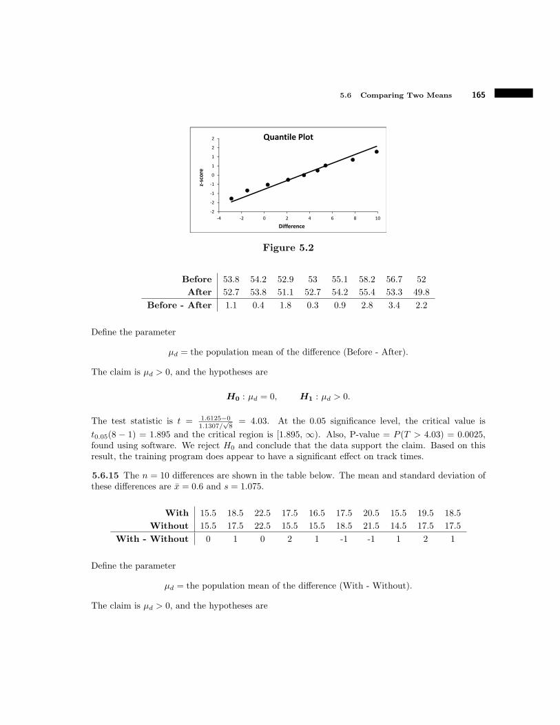
5.6 Comparing Two Means 165
-2
-2
-1
-1
0
1
1
2
2
-4 -2 0 2 4 6 8 10
z-sc
ore
Difference
Quantile Plot
Figure 5.2
Before 53.8 54.2 52.9 53 55.1 58.2 56.7 52
After 52.7 53.8 51.1 52.7 54.2 55.4 53.3 49.8
Before - After 1.1 0.4 1.8 0.3 0.9 2.8 3.4 2.2
Define the parameter
µd = the population mean of the di!erence (Before - After).
The claim is µd > 0, and the hypotheses are
H0 : µd = 0, H1 : µd > 0.
The test statistic is t = 1.6125!01.1307/
'8
= 4.03. At the 0.05 significance level, the critical value is
t0.05(8 # 1) = 1.895 and the critical region is [1.895, 0). Also, P-value = P (T > 4.03) = 0.0025,found using software. We reject H0 and conclude that the data support the claim. Based on thisresult, the training program does appear to have a significant e!ect on track times.
5.6.15 The n = 10 di!erences are shown in the table below. The mean and standard deviation ofthese di!erences are x = 0.6 and s = 1.075.
With 15.5 18.5 22.5 17.5 16.5 17.5 20.5 15.5 19.5 18.5
Without 15.5 17.5 22.5 15.5 15.5 18.5 21.5 14.5 17.5 17.5
With - Without 0 1 0 2 1 -1 -1 1 2 1
Define the parameter
µd = the population mean of the di!erence (With - Without).
The claim is µd > 0, and the hypotheses are

166 CHAPTER 5 Hypothesis Testing
H0 : µd = 0, H1 : µd > 0.
The test statistic is t = 0.6!01.075/
'10
= 1.76. At the 0.05 significance level, the critical value is
t0.05(10 # 1) = 1.833 and the critical region is [1.833, 0). Also, P-value = P (T > 1.76) = 0.0561,found using software. We do not reject H0 and conclude that the data do not support the claim.Based on this result, shoes do not appear to have a significant a!ect at the 0.05 significance level.
5.6.16 The n = 12 di!erences are shown in the table below. The mean and standard deviation ofthese di!erences are x = 0.4083 and s = 0.4562.
Reported 67 73 67.5 70 68 70 71 68 67.5 66 70 71.5
Measured 66.3 72.8 68 69.4 67.3 70.2 70.9 67.6 67.1 65.3 68.8 70.9
Reported - Measured 0.7 0.2 -0.5 0.6 0.7 -0.2 0.1 0.4 0.4 0.7 1.2 0.6
Define the parameter
µd = the population mean of the di!erence (Reported - Measured).
The claim is µd > 0, and the hypotheses are
H0 : µd = 0, H1 : µd > 0.
The test statistic is t = 0.4083!00.4562/
'12
= 3.10. At the 0.05 significance level, the critical value is
t0.05(12 # 1) = 1.796 and the critical region is [1.796, 0). Also, P-value = P (T > 3.10) = 0.0051,found using software. We reject H0 and conclude that the data support the claim. Students mayhave just been rounding up to the next whole number.
5.6.17 The n = 6 di!erences are shown in the table below. The mean and standard deviation ofthese di!erences are x = #0.8833 and s = 0.9948.
Bi-metallic 87.5 82.9 59.2 49.2 42.7 32.9
Infrared 88.7 83.7 61.9 49.1 43.1 33.2
Bi-metallic - Infrared -1.2 -0.8 -2.7 0.1 -0.4 -0.3
Define the parameter
µd = the population mean of the di!erence (Bi-metallic - Infared).
We test the claim µd = 0, and the hypotheses are
H0 : µd = 0, H1 : µd += 0.

5.6 Comparing Two Means 167
The test statistic is t = !0.8833!00.9948/
'6
= #2.17. At the 0.05 significance level, the critical value is
t0.05/2(6#1) = 2.571 and the critical region is (#0, #2.571]( [2.571, 0). Also, P-value = 2 ·P (T <#2.17) = 0.0821, found using software. We do not reject H0 and conclude that there is not su"cientevidence to reject the claim. Thus there does not appear to be a significant di!erence between thetemperature readings of the two types of thermometers.
5.6.18 The parameters are
µ1 = The mean amount of sodium in all generic cereals, and
µ2 = The mean amount of sodium in all brand-name cereals.
a. Since both sample sizes are greater than 30, we construct Z-intervals. The calculations aresummarized in the table below. Since these intervals overlap, there does not appear to be asignificant di!erence between the population means.
n x s E C.I.
Generic 62 158.22 73.30 15.31 142.91 < µ1 < 173.5
Brand-name 74 137.79 60.69 11.6 126.19 < µ2 < 149.39
b. Since both sample sizes are greater than 30, we perform a Z-test with the alternative hypothesisH1 : µ1 # µ2 += 0. The test statistic is
z =(158.22# 137.79)# 0/73.32/62 + 60.692/74
= 1.75.
At the 0.10 significance level, the critical value is z0.10 = 1.282 and the critical region is(#0, #1.282]( [1.282, 0). Also, P-value = 2 ·P (Z > 1.75) = 0.0802. Thus we reject H0 andconclude that there is su"cient evidence to reject the claim. Thus there does appear to be adi!erence between these two population means. This is a di!erent conclusion reached than inpart a.
5.6.19
a. Quantile plots of the data are shown in Figure 5.3. Based on these plots, it appears that bothpopulations are normally distributed.
b. These data have the same summary statistics as in exercise 5.5.10, so we come to the sameconclusion as in that exercise: There is not su"cient evidence to reject the claim of equalpopulation variances.
c. The parameters are
µ1 = The mean mass of all blue candies, and
µ2 = The mean mass of all red candies.
The claim is µ1 # µ2 > 0, so we test the hypotheses

168 CHAPTER 5 Hypothesis Testing
-2
-2
-1
-1
0
1
1
2
2
0.74 0.76 0.78 0.8 0.82 0.84 0.86
z-sc
ore
Mass
Quantile Plot for Red
-3-2
-2-1
-1
01
12
2
0.85 0.86 0.87 0.88 0.89 0.9 0.91 0.92 0.93 0.94
z-sc
ore
Mass
Quantile Plot for Blue
Figure 5.3
H0 : µ1 # µ2 = 0, H1 : µ1 # µ2 > 0.
From the data we get n1 = n2 = 13, x1 = 0.8935, s1 = 0.0190, x2 = 0.8022, and s2 = 0.0224so
sp =
J(13# 1) 0.0192 + (13# 1) 0.02242
13 + 13# 2= 0.0207, t =
(0.8935# 0.8022)# 0
0.0207/1/13 + 1/13
= 11.24.
At the 95% confidence level, the critical value is t0.05(13 + 13 # 2) = 1.711 and the criticalregion is [1.711, 0). Also, P-value = P (T > 11.24) = 0.000. Thus we reject H0 and concludethat the data support the claim.
5.6.20 From the data, we get m1 = 7.77 and m2 = 8.15. The transformed values are shown in thetable below.
Sample 1 5.66 6.62 6.76 7.58 7.66 7.77 7.95 8.38 8.38 8.05 9.13
|x!m1| 2.11 1.15 1.01 0.19 0.11 0 0.18 0.61 0.61 0.73 1.36
Sample 2 7.41 7.62 7.63 7.73 7.84 8.15 8.26 8.27 8.46 8.54 8.75
|x!m2| 0.74 0.53 0.52 0.42 0.31 0 0.11 0.12 0.31 0.39 0.6
The parameters are
µ1 = The mean of the transformed values in the first population, and
µ2 = The mean of the transformed values in the second population.
The claim is µ1 # µ2 = 0, so we test the hypotheses
H0 : µ1 # µ2 = 0, H1 : µ1 # µ2 += 0.