BASICS ON BASES:BASICS ON BASES:

AA--GG--TT--C AS WORDSC AS WORDS

582606 Introduction to Bioinformatics, Autumn 2009 10. Sept / 1

Sirkka-Liisa Varvio

The bases Adenine, Guanine, Thymine, and Cytosine formchemical pairs A-T and C-G DNA double helix

This lecture approaches the DNA-world by considering words, short stringsof letters drawn from an alphabet, which in the case DNA is the set of lettersA-G-T-C forming k-words or k- tuples (k is the word length).

DNA sequences from different regions of a genome differ by their k-tuplecontent and different organisms differ as well.

We take a look at computational issues on words, how to count words andhow words can be located along a string.

Word distribution description includes probabilistic modelling.

Some statistics used to describe word frequencies.

Sirkka-Liisa Varvio

582606 Introduction to Bioinformatics, Autumn 2009 10. Sept / 2

Next week lectures:

The biological perspective on DNA-world and A-G-T-C.

Flow of biological information, DNA, RNA, proteins

Next week also Biology for methodological scientists: The reading group inMeilahti campus starts (Wednesday, see the calendar and course list).

In the the wet-lab biology course, Measurement techniques, you extractDNA from yourselves in Wednesday 23. September.

3

A cell of an organism contains DNA-molecules,organized into chromosomes

Organism #base pairs #chromosomes

Escherichia coli (bacterium) 4x106 1Saccharomyces cerevisiae (yeast) 1.35x107 17Drosophila melanogaster (insect) 1.65x108 4Homo sapiens (human) 2.9x109 23Zea mays (corn / maize) 5.0x109 10

582606 Introduction to Bioinformatics, Autumn 2009 10. Sept / 3

Sirkka-Liisa Varvio

4

DNA codes for proteins

• The DNA-code A-G-T-C throughRNA-code, A-G-U-C, codes for 20different amino acids.

• Trinucleotides (triplets) allow 43 =64 possible trinucleotides.

• Triplets are also called codons.

582606 Introduction to Bioinformatics, Autumn 2009 10. Sept / 4

Sirkka-Liisa Varvio

5

DNA makes new copies of itself, replicates

• In this process, mistakes can occur.

• The cell repair machinery may, or may not, correct the mistakes.

• Mistakes can be moved on as mutations.

• This in one (simple) mechanism that generates differences to DNA-differences between organisms.

• This is can be considered as a string manipulation issue

582606 Introduction to Bioinformatics, Autumn 2009 10. Sept / 5

Sirkka-Liisa Varvio

6

Biological string manipulation

• One type of a mutation is deletion: removal of one or more contiguousbases (substring)– …TTGATCA… => …TTTCA…

• Another type is and insertion: insertion of a substring– …GGCTAG… => …GGTCAACTAG…

• Point mutation: substitution of a base– …ACGGCT… => …ACGCCT…

582606 Introduction to Bioinformatics, Autumn 2009 10. Sept / 6

Sirkka-Liisa Varvio

7

1 atgagccaag ttccgaacaa ggattcgcgg ggaggataga tcagcgcccg agaggggtga61 gtcggtaaag agcattggaa cgtcggagat acaactccca agaaggaaaa aagagaaagc

121 aagaagcgga tgaatttccc cataacgcca gtgaaactct aggaagggga aagagggaag181 gtggaagaga aggaggcggg cctcccgatc cgaggggccc ggcggccaag tttggaggac241 actccggccc gaagggttga gagtacccca gagggaggaa gccacacgga gtagaacaga301 gaaatcacct ccagaggacc ccttcagcga acagagagcg catcgcgaga gggagtagac361 catagcgata ggaggggatg ctaggagttg ggggagaccg aagcgaggag gaaagcaaag421 agagcagcgg ggctagcagg tgggtgttcc gccccccgag aggggacgag tgaggcttat481 cccggggaac tcgacttatc gtccccacat agcagactcc cggaccccct ttcaaagtga541 ccgagggggg tgactttgaa cattggggac cagtggagcc atgggatgct cctcccgatt601 ccgcccaagc tccttccccc caagggtcgc ccaggaatgg cgggacccca ctctgcaggg661 tccgcgttcc atcctttctt acctgatggc cggcatggtc ccagcctcct cgctggcgcc721 ggctgggcaa cattccgagg ggaccgtccc ctcggtaatg gcgaatggga cccacaaatc781 tctctagctt cccagagaga agcgagagaa aagtggctct cccttagcca tccgagtgga841 cgtgcgtcct ccttcggatg cccaggtcgg accgcgagga ggtggagatg ccatgccgac901 ccgaagagga aagaaggacg cgagacgcaa acctgcgagt ggaaacccgc tttattcact961 ggggtcgaca actctgggga gaggagggag ggtcggctgg gaagagtata tcctatggga

1021 atccctggct tccccttatg tccagtccct ccccggtccg agtaaagggg gactccggga1081 ctccttgcat gctggggacg aagccgcccc cgggcgctcc cctcgttcca ccttcgaggg1141 ggttcacacc cccaacctgc gggccggcta ttcttctttc ccttctctcg tcttcctcgg1201 tcaacctcct aagttcctct tcctcctcct tgctgaggtt ctttcccccc gccgatagct1261 gctttctctt gttctcgagg gccttccttc gtcggtgatc ctgcctctcc ttgtcggtga1321 atcctcccct ggaaggcctc ttcctaggtc cggagtctac ttccatctgg tccgttcggg1381 ccctcttcgc cgggggagcc ccctctccat ccttatcttt ctttccgaga attcctttga1441 tgtttcccag ccagggatgt tcatcctcaa gtttcttgat tttcttctta accttccgga1501 ggtctctctc gagttcctct aacttctttc ttccgctcac ccactgctcg agaacctctt1561 ctctcccccc gcggtttttc cttccttcgg gccggctcat cttcgactag aggcgacggt1621 cctcagtact cttactcttt tctgtaaaga ggagactgct ggccctgtcg cccaagttcg1681 ag

Given a DNA sequence, we might ask a number of questions

What sort of statistics should be used to describe the sequence?

What sort of organism did this sequence come from?

Does the description of this sequence differ fromthe description of other DNA in the organism?

What sort of sequence is this? What does it do?

582606 Introduction to Bioinformatics, Autumn 2009 10. Sept / 7

From: Esa Pitkänen

8

Biological words

• We can try to answer questions like these by considering the words in asequence

• A k-word (or a k-tuple) is a string of length k drawn from some alphabet

• A DNA k-word is a string of length k that consists of letters A, C, G, T– 1-words: individual nucleotides (bases)– 2-words: dinucleotides (AA, AC, AG, AT, CA, ...)– 3-words: codons (AAA, AAC, …)– 4-words and beyond

582606 Introduction to Bioinformatics, Autumn 2009 10. Sept / 8

From: Esa Pitkänen

9

1-words: base composition

• Typically DNA exists as duplex molecule (two complementary strands)

5’-GGATCGAAGCTAAGGGCT-3’3’-CCTAGCTTCGATTCCCGA-5’

Top strand: 7 G, 3 C, 5 A, 3 TBottom strand: 3 G, 7 C, 3 A, 5 TDuplex molecule: 10 G, 10 C, 8 A, 8 TBase frequencies: 10/36 10/36 8/36 8/36

fr(G + C) = 20/36, fr(A + T) = 1 – fr(G + C) = 16/36

These are somethingwe can determineexperimentally.

582606 Introduction to Bioinformatics, Autumn 2009 10. Sept / 9

From: Esa Pitkänen

10

G+C content

• fr(G + C), or G+C content is a simple statistics for describing genomes

• Notice that one value is enough characterise fr(A), fr(C), fr(G) and fr(T) forduplex DNA

• Is G+C content (= base composition) able to tell the difference betweengenomes of different organisms?

– Simple computational experiment, if we have the genome sequencesunder study (-> exercises)

582606 Introduction to Bioinformatics, Autumn 2009 10. Sept / 10

From: Esa Pitkänen

11

G+C content for various organisms

Bacteria• Mycoplasma genitalium 31.6%• Escherichia coli K-12 50.7%• Pseudomonas aeruginosa PAO1 66.4%• Pyrococcus abyssi 44.6%• Thermoplasma volcanium 39.9%worm• Caenorhabditis elegans 36%plant• Arabidopsis thaliana 35%human• Homo sapiens 41%

582606 Introduction to Bioinformatics, Autumn 2009 10. Sept / 11

From: Esa Pitkänen

12

Base frequencies in duplex molecules

• Consider a DNA sequence generated randomly, with probability of eachletter being independent of position in sequence

• You could expect to find a uniform distribution of bases in genomes…

• This is not, however, the case in genomes, especially in bacteria

– This phenomenon is called GC skew

5’-...GGATCGAAGCTAAGGGCT...-3’3’-...CCTAGCTTCGATTCCCGA...-5’

582606 Introduction to Bioinformatics, Autumn 2009 10. Sept / 12

From: Esa Pitkänen

13

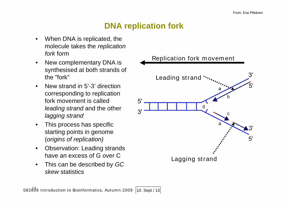
DNA replication fork• When DNA is replicated, the

molecule takes the replicationfork form

• New complementary DNA issynthesised at both strands ofthe ”fork”

• New strand in 5’-3’ directioncorresponding to replicationfork movement is calledleading strand and the otherlagging strand

• This process has specificstarting points in genome(origins of replication)

• Observation: Leading strandshave an excess of G over C

• This can be described by GCskew statistics

Leading strand

Lagging strand

Replication fork movement

582606 Introduction to Bioinformatics, Autumn 2009 10. Sept / 13

From: Esa Pitkänen

14

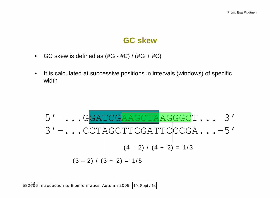
GC skew

• GC skew is defined as (#G - #C) / (#G + #C)

• It is calculated at successive positions in intervals (windows) of specificwidth

5’-...GGATCGAAGCTAAGGGCT...-3’3’-...CCTAGCTTCGATTCCCGA...-5’

(3 – 2) / (3 + 2) = 1/5

(4 – 2) / (4 + 2) = 1/3

582606 Introduction to Bioinformatics, Autumn 2009 10. Sept / 14

From: Esa Pitkänen

15

• G-C content & GC skewstatistics can bedisplayed with a circulargenome map

Chromosome map of S. dysenteriae, the nine ringsdescribe different properties of the genomehttp://www.mgc.ac.cn/ShiBASE/circular_Sd197.htm

G-C content & GC skew

G+C content

GC skew

(10kb window size)

582606 Introduction to Bioinformatics, Autumn 2009 10. Sept / 1

From: Esa Pitkänen

16

GC skew• GC skew often

changes sign atorigins and terminiof replication

G+C content

GC skew

(10kb window size)

Nie et al., BMC Genomics, 2006582606 Introduction to Bioinformatics, Autumn 2009 10. Sept / 16

From: Esa Pitkänen

17

2-words: dinucleotides

• Let’s consider a sequence L1,L2,...,Ln where each letter Li is drawn from theDNA alphabet {A, C, G, T}

• We have 16 possible dinucleotides lili+1: AA, AC, AG, ..., TG, TT.

582606 Introduction to Bioinformatics, Autumn 2009 10. Sept / 17

From: Esa Pitkänen

18

i.i.d. model for nucleotides

• Assume that bases– occur independently of each other– bases at each position are identically distributed

• Probability of the base A, C, G, T occuring is pA, pC, pG, pT, respectively– For example, we could use pA=pC=pG=pT=0.25 or estimate the values

from known genome data

• Probability of lili+1 is then PliPli+1

– For example, P(TG) = pT pG

582606 Introduction to Bioinformatics, Autumn 2009 10. Sept / 18

From: Esa Pitkänen

What is i.i.d ?

In probability theory and statistics asequence or other collection of randomvariables is

independent and identically distributed(i.i.d.) if each random variable has the sameprobability distribution as the others and allare mutually independent.

19

2-words: is what we see surprising?

• We can test whether a sequence is ”unexpected”, for example, with a 2 test

• Test statistic for a particular dinucleotide r1r2 is 2 = (O – E)2 / E where– O is the observed number of dinucleotide r1r2– E is the expected number of dinucleotide r1r2– E = (n – 1)pr1pr2 under i.i.d. model

• Basic idea: high values of 2 indicate deviation from the model– Actual procedure is more detailed -> basic statistics courses

582606 Introduction to Bioinformatics, Autumn 2009 10. Sept / 19

From: Esa Pitkänen

20

Refining the i.i.d. model

• i.i.d. model describes some organisms well but fails to characterise manyothers

• We can refine the model by having the DNA letter at some position dependon letters at preceding positions

…TCGTGACGCCG ?

Sequence context toconsider

582606 Introduction to Bioinformatics, Autumn 2009 10. Sept / 20

From: Esa Pitkänen

21

First-order Markov chains

• Lets assume that in sequence X the letter at position t, Xt, depends only onthe previous letter Xt-1 (first-order markov chain)

• Probability of letter j occuring at position t given Xt-1 = i: pij = P(Xt = j | Xt-1 = i)

• We consider homogeneous Markov chains: probability pij is independent ofposition t

…TCGTGACGCCG ?

Xt

Xt-1

582606 Introduction to Bioinformatics, Autumn 2009 10. Sept / 21

From: Esa Pitkänen

22

Estimating pij

• We can estimate probabilities pij (”the probability that j follows i”) fromobserved dinucleotide frequencies

A C G TA pAA pAC pAG pATC pCA pCC pCG pCTG pGA pGC pGG pGTT pTA pTC pTG pTT

Frequencyof dinucleotide ATin sequence

…the values pAA, pAC, ..., pTG, pTT sum to 1

+ + + Base frequencyfr(C)

582606 Introduction to Bioinformatics, Autumn 2009 10. Sept / 22

From: Esa Pitkänen

23

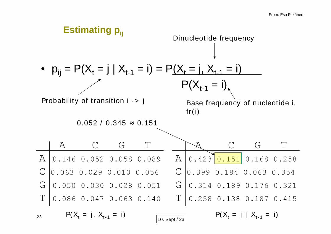
Estimating pij

• pij = P(Xt = j | Xt-1 = i) = P(Xt = j, Xt-1 = i)P(Xt-1 = i)

Probability of transition i -> j

Dinucleotide frequency

Base frequency of nucleotide i,fr(i)

A C G TA 0.146 0.052 0.058 0.089

C 0.063 0.029 0.010 0.056

G 0.050 0.030 0.028 0.051

T 0.086 0.047 0.063 0.140

P(Xt = j, Xt-1 = i)

A C G TA 0.423 0.151 0.168 0.258

C 0.399 0.184 0.063 0.354

G 0.314 0.189 0.176 0.321

T 0.258 0.138 0.187 0.415

P(Xt = j | Xt-1 = i)

0.052 / 0.345 0.151

10. Sept / 23

From: Esa Pitkänen

24

Simulating a DNA sequence

• From a transition matrix, it is easy to generate a DNA sequence of length n:– First, choose the starting base randomly according to the base

frequency distribution– Then, choose next base according to the distribution P(xt | xt-1) until n

bases have been chosen

A C G TA 0.423 0.151 0.168 0.258

C 0.399 0.184 0.063 0.354

G 0.314 0.189 0.176 0.321

T 0.258 0.138 0.187 0.415

P(Xt = j | Xt-1 = i)

T T C T T C AA

582606 Introduction to Bioinformatics, Autumn 2009 10. Sept / 24

From: Esa Pitkänen

25

ttcttcaaaataaggatagtgattcttattggcttaagggataacaatttagatcttttttcatgaatcatgtatgtcaacgttaaaagttgaactgcaataagttcttacacacgattgtttatctgcgtgcgaagcatttcactacatttgccgatgcagccaaaagtatttaacatttggtaaacaaattgacttaaatcgcgcacttagagtttgacgtttcatagttgatgcgtgtctaacaattacttttagttttttaaatgcgtttgtctacaatcattaatcagctctggaaaaacattaatgcatttaaaccacaatggataattagttacttattttaaaattcacaaagtaattattcgaatagtgccctaagagagtactggggttaatggcaaagaaaattactgtagtgaagattaagcctgttattatcacctgggtactctggtgaatgcacataagcaaatgctacttcagtgtcaaagcaaaaaaatttactgataggactaaaaaccctttatttttagaatttgtaaaaatgtgacctcttgcttataacatcatatttattgggtcgttctaggacactgtgattgccttctaactcttatttagcaaaaaattgtcatagctttgaggtcagacaaacaagtgaatggaagacagaaaaagctcagcctagaattagcatgttttgagtggggaattacttggttaactaaagtgttcatgactgttcagcatatgattgttggtgagcactacaaagatagaagagttaaactaggtagtggtgatttcgctaacacagttttcatacaagttctattttctcaatggttttggataagaaaacagcaaacaaatttagtattattttcctagtaaaaagcaaacatcaaggagaaattggaagctgcttgttcagtttgcattaaattaaaaatttatttgaagtattcgagcaatgttgacagtctgcgttcttcaaataagcagcaaatcccctcaaaattgggcaaaaacctaccctggcttctttttaaaaaaccaagaaaagtcctatataagcaacaaatttcaaaccttttgttaaaaattctgctgctgaataaataggcattacagcaatgcaattaggtgcaaaaaaggccatcctctttctttttttgtacaattgttcaagcaactttgaatttgcagattttaacccactgtctatatgggacttcgaattaaattgactggtctgcatcacaaatttcaactgcccaatgtaatcatattctagagtattaaaaatacaaaaagtacaattagttatgcccattggcctggcaatttatttactccactttccacgttttggggatattttaacttgaatagttcacaatcaaaacataggaaggatctactgctaaaagcaaaagcgtattggaatgataaaaaactttgatgtttaaaaaactacaaccttaatgaattaaagttgaaaaaatattcaaaaaaagaaattcagttcttggcgagtaatatttttgatgtttgagatcagggttacaaaataagtgcatgagattaactcttcaaatataaactgatttaagtgtatttgctaataacattttcgaaaaggaatattatggtaagaattcataaaaatgtttaatactgatacaactttcttttatatcctccatttggccagaatactgttgcacacaactaattggaaaaaaaatagaacgggtcaatctcagtgggaggagaagaaaaaagttggtgcaggaaatagtttctactaacctggtataaaaacatcaagtaacattcaaattgcaaatgaaaactaaccgatctaagcattgattgatttttctcatgcctttcgcctagttttaataaacgcgccccaactctcatcttcggttcaaatgatctattgtatttatgcactaacgtgcttttatgttagcatttttcaccctgaagttccgagtcattggcgtcactcacaaatgacattacaatttttctatgttttgttctgttgagtcaaagtgcatgcctacaattctttcttatatagaactagacaaaatagaaaaaggcacttttggagtctgaatgtcccttagtttcaaaaaggaaattgttgaattttttgtggttagttaaattttgaacaaactagtatagtggtgacaaacgatcaccttgagtcggtgactataaaagaaaaaggagattaaaaatacctgcggtgccacattttttgttacgggcatttaaggtttgcatgtgttgagcaattgaaacctacaactcaataagtcatgttaagtcacttctttgaaaaaaaaaaagaccctttaagcaagctc

.

582606 Introduction to Bioinformatics, Autumn 2009 10. Sept / 25

From: Esa Pitkänen

Now we can quickly generate sequences of arbitrarylength...

26

Results from simulating a DNA sequence

aa 0.145 0.146ac 0.050 0.052ag 0.055 0.058at 0.092 0.089ca 0.065 0.063cc 0.028 0.029cg 0.011 0.010ct 0.058 0.056ga 0.048 0.050gc 0.032 0.030gg 0.029 0.028gt 0.050 0.051ta 0.084 0.086tc 0.052 0.047tg 0.064 0.063tt 0.138 0.0140

Dinucleotide frequenciesSimulated Observed

n = 10000

582606 Introduction to Bioinformatics, Autumn 2009 10. Sept / 26

From: Esa Pitkänen

27

Simulating a DNA sequence

ttcttcaaaataaggatagtgattcttattggcttaagggataacaatttagatcttttttcatgaatcatgtatgtcaacgttaaaagttgaactgcaataagttcttacacacgattgtttatctgcgtgcgaagcatttcactacatttgccgatgcagccaaaagtatttaacatttggtaaacaaattgacttaaatcgcgcacttagagtttgacgtttcatagttgatgcgtgtctaacaattacttttagttttttaaatgcgtttgtctacaatcattaatcagctctggaaaaacattaatgcatttaaaccacaatggataattagttacttattttaaaattcacaaagtaattattcgaatagtgccctaagagagtactggggttaatggcaaagaaaattactgtagtgaagattaagcctgttattatcacctgggtactctggtgaatgcacataagcaaatgctacttcagtgtcaaagcaaaaaaatttactgataggactaaaaaccctttatttttagaatttgtaaaaatgtgacctcttgcttataacatcatatttattgggtcgttctaggacactgtgattgccttctaactcttatttagcaaaaaattgtcatagctttgaggtcagacaaacaagtgaatggaagacagaaaaagctcagcctagaattagcatgttttgagtggggaattacttggttaactaaagtgttcatgactgttcagcatatgattgttggtgagcactacaaagatagaagagttaaactaggtagtggtgatttcgctaacacagttttcatacaagttctattttctcaatggttttggataagaaaacagcaaacaaatttagtattattttcctagtaaaaagcaaacatcaaggagaaattggaagctgcttgttcagtttgcattaaattaaaaatttatttgaagtattcgagcaatgttgacagtctgcgttcttcaaataagcagcaaatcccctcaaaattgggcaaaaacctaccctggcttctttttaaaaaaccaagaaaagtcctatataagcaacaaatttcaaaccttttgttaaaaattctgctgctgaataaataggcattacagcaatgcaattaggtgcaaaaaaggccatcctctttctttttttgtacaattgttcaagcaactttgaatttgcagattttaacccactgtctatatgggacttcgaattaaattgactggtctgcatcacaaatttcaactgcccaatgtaatcatattctagagtattaaaaatacaaaaagtacaattagttatgcccattggcctggcaatttatttactccactttccacgttttggggatattttaacttgaatagttcacaatcaaaacataggaaggatctactgctaaaagcaaaagcgtattggaatgataaaaaactttgatgtttaaaaaactacaaccttaatgaattaaagttgaaaaaatattcaaaaaaagaaattcagttcttggcgagtaatatttttgatgtttgagatcagggttacaaaataagtgcatgagattaactcttcaaatataaactgatttaagtgtatttgctaataacattttcgaaaaggaatattatggtaagaattcataaaaatgtttaatactgatacaactttcttttatatcctccatttggccagaatactgttgcacacaactaattggaaaaaaaatagaacgggtcaatctcagtgggaggagaagaaaaaagttggtgcaggaaatagtttctactaacctggtataaaaacatcaagtaacattcaaattgcaaatgaaaactaaccgatctaagcattgattgatttttctcatgcctttcgcctagttttaataaacgcgccccaactctcatcttcggttcaaatgatctattgtatttatgcactaacgtgcttttatgttagcatttttcaccctgaagttccgagtcattggcgtcactcacaaatgacattacaatttttctatgttttgttctgttgagtcaaagtgcatgcctacaattctttcttatatagaactagacaaaatagaaaaaggcacttttggagtctgaatgtcccttagtttcaaaaaggaaattgttgaattttttgtggttagttaaattttgaacaaactagtatagtggtgacaaacgatcaccttgagtcggtgactataaaagaaaaaggagattaaaaatacctgcggtgccacattttttgttacgggcatttaaggtttgcatgtgttgagcaattgaaacctacaactcaataagtcatgttaagtcacttctttgaaaaaaaaaaagaccctttaagcaagctc

• The model is able to generate correct proportions of 1- and 2-words ingenomes...

• ...but fails with k=3 and beyond.

582606 Introduction to Bioinformatics, Autumn 2009 10. Sept /27

From: Esa Pitkänen

28

3-words: codons

• We can extend the previous method to 3-words

• k=3 is an important case in study of DNA sequences because of geneticcode

5’ 3’

3’ 5’

… a t g a g t g g a …

… t a c t c a c c t …

a u g a g u g g a ...

M S G …

582606 Introduction to Bioinformatics, Autumn 2009 10. Sept / 28

From: Esa Pitkänen

29

3-word probabilities

• Let’s again assume a sequence L of independent bases

• Probability of 3-word r1r2r3 at position i,i+1,i+2 in sequence L is

P(Li = r1, Li+1 = r2, Li+2 = r3) =

P(Li = r1)P(Li+1 = r2)P(Li+2 = r3)

582606 Introduction to Bioinformatics, Autumn 2009 10. Sept / 29

From: Esa Pitkänen

30

3-words in Escherichia coli genome

AAA 108924 0.02348 0.01492AAC 82582 0.01780 0.01541AAG 63369 0.01366 0.01537AAT 82995 0.01789 0.01490ACA 58637 0.01264 0.01541ACC 74897 0.01614 0.01591ACG 73263 0.01579 0.01588ACT 49865 0.01075 0.01539AGA 56621 0.01220 0.01537AGC 80860 0.01743 0.01588AGG 50624 0.01091 0.01584AGT 49772 0.01073 0.01536ATA 63697 0.01373 0.01490ATC 86486 0.01864 0.01539ATG 76238 0.01643 0.01536ATT 83398 0.01797 0.01489

CAA 76614 0.01651 0.01541CAC 66751 0.01439 0.01591CAG 104799 0.02259 0.01588CAT 76985 0.01659 0.01539CCA 86436 0.01863 0.01591CCC 47775 0.01030 0.01643CCG 87036 0.01876 0.01640CCT 50426 0.01087 0.01589CGA 70938 0.01529 0.01588CGC 115695 0.02494 0.01640CGG 86877 0.01872 0.01636CGT 73160 0.01577 0.01586CTA 26764 0.00577 0.01539CTC 42733 0.00921 0.01589CTG 102909 0.02218 0.01586CTT 63655 0.01372 0.01537

Word Count Observed Expected Word Count Observed Expected

582606 Introduction to Bioinformatics, Autumn 2009 10. Sept / 30

From: Esa Pitkänen

31

2nd order Markov Chains• Markov chains readily generalise to higher orders• In 2nd order markov chain, position t depends on positions t-1 and t-2• Transition matrix:

A C G TAAACAGATCA...

582606 Introduction to Bioinformatics, Autumn 2009 10. Sept / 31

From: Esa Pitkänen

32

Codon Adaptation Index (CAI)

• Observation: cells prefer certain codons over others in highly expressedgenes– Gene expression: DNA is transcribed into RNA (and possibly translated

into protein)• CAI is a statistic used to compare the distribution of codons

observed with the preferred codons for highly expressed genes

Phe TTT 0.493 0.551 0.291TTC 0.507 0.449 0.709

Ala GCT 0.246 0.145 0.275GCC 0.254 0.276 0.164GCA 0.246 0.196 0.240GCG 0.254 0.382 0.323

Asn AAT 0.493 0.409 0.172AAC 0.507 0.591 0.828

Aminoacid Codon Predicted Gene class I Gene class II

Highlyexpressed

Moderatelyexpressed

Codon frequencies for some genes in E. coli582606 Introduction to Bioinformatics, Autumn 2009 10. Sept / 32

From: Esa Pitkänen

33

Codon Adaptation Index (CAI)• Consider an amino acid sequence X = x1x2...xn

• Let pk be the probability that codon k is used in highly expressed genes

• Let qk be the highest probability that a codon coding for the same aminoacid as codon k has

– For example, if codon k is ”GCC”, the corresponding amino acid isAlanine (see genetic code table; also GCT, GCA, GCG code forAlanine)

– Assume that pGCC = 0.164, pGCT = 0.275, pGCA = 0.240, pGCG = 0.323

– Now qGCC = qGCT = qGCA = qGCG = 0.323

582606 Introduction to Bioinformatics, Autumn 2009 10. Sept / 33

From: Esa Pitkänen

34

Codon Adaptation Index (CAI)

• CAI is defined as

• CAI can be given also in log-odds form:

log(CAI) = (1/n) log(pk / qk)

CAI = ( pk / qk )k=1

n 1/n

k=1

n

582606 Introduction to Bioinformatics, Autumn 2009 10. Sept / 34

From: Esa Pitkänen

35

CAI: example with an E. coli gene

M A L T K A E M S E Y L …ATG GCG CTT ACA AAA GCT GAA ATG TCA GAA TAT CTG1.00 0.47 0.02 0.45 0.80 0.47 0.79 1.00 0.43 0.79 0.19 0.02

0.06 0.02 0.47 0.20 0.06 0.21 0.32 0.21 0.81 0.020.28 0.04 0.04 0.28 0.03 0.040.20 0.03 0.05 0.20 0.01 0.03

0.01 0.04 0.010.89 0.18 0.89

ATG GCT TTA ACT AAA GCT GAA ATG TCT GAA TAT TTAGCC TTG ACC AAG GCC GAG TCC GAG TAC TTGGCA CTT ACA GCA TCA CTTGCG CTC ACG GCG TCG CTC

CTA AGT CTACTG AGC CTG

1.00 0.20 0.04 0.04 0.80 0.47 0.79 1.00 0.03 0.79 0.19 0.89…1.00 0.47 0.89 0.47 0.80 0.47 0.79 1.00 0.43 0.79 0.81 0.89

1/n

qkpk

582606 Introduction to Bioinformatics, Autumn 2009 10. Sept / 35

From: Esa Pitkänen

36

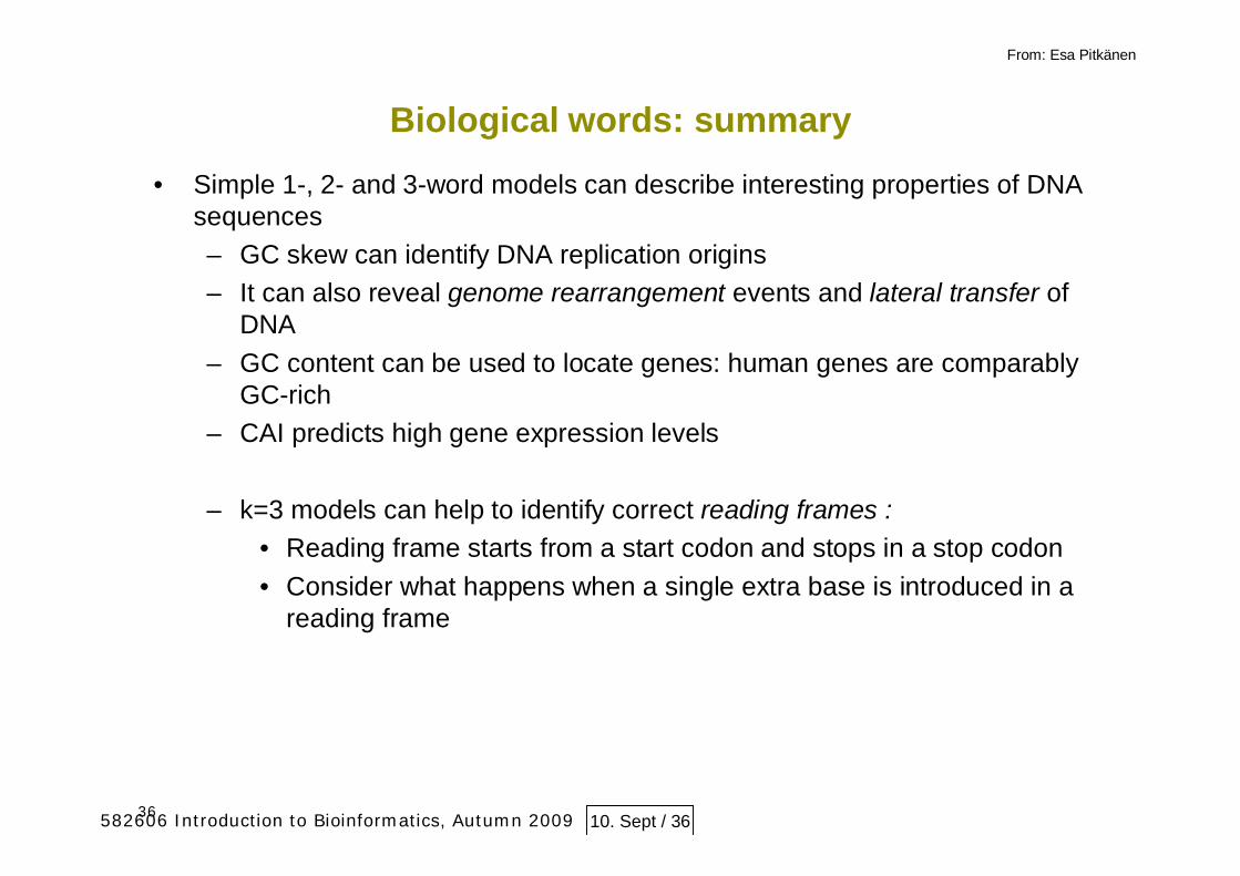
Biological words: summary

• Simple 1-, 2- and 3-word models can describe interesting properties of DNAsequences– GC skew can identify DNA replication origins– It can also reveal genome rearrangement events and lateral transfer of

DNA– GC content can be used to locate genes: human genes are comparably

GC-rich– CAI predicts high gene expression levels

– k=3 models can help to identify correct reading frames :• Reading frame starts from a start codon and stops in a stop codon• Consider what happens when a single extra base is introduced in a

reading frame

582606 Introduction to Bioinformatics, Autumn 2009 10. Sept / 36

From: Esa Pitkänen

37

Note on programming languages

• Working with probability distributions is straightforward with R.

• You can use R in Computer science classrooms Linux systems

• Python works too!

582606 Introduction to Bioinformatics, Autumn 2009 10. Sept / 37

From: Esa Pitkänen

38

#!/usr/bin/env python

import sys, random

n = int(sys.argv[1])

tm = {'a' : {'a' : 0.423, 'c' : 0.151, 'g' : 0.168, 't' : 0.258},'c' : {'a' : 0.399, 'c' : 0.184, 'g' : 0.063, 't' : 0.354},'g' : {'a' : 0.314, 'c' : 0.189, 'g' : 0.176, 't' : 0.321},'t' : {'a' : 0.258, 'c' : 0.138, 'g' : 0.187, 't' : 0.415}}

pi = {'a' : 0.345, 'c' : 0.158, 'g' : 0.159, 't' : 0.337}

def choose(dist):r = random.random()sum = 0.0keys = dist.keys()for k in keys:

sum += dist[k]if sum > r:

return kreturn keys[-1]

c = choose(pi)for i in range(n - 1):

sys.stdout.write(c)c = choose(tm[c])

sys.stdout.write(c)sys.stdout.write("\n")

Example Python code for generatingDNA sequences with first-orderMarkov chains.

Function choose(), returns a key (here ’a’, ’c’, ’g’ or’t’) of the dictionary ’dist’ chosen randomlyaccording to probabilities in dictionary values.

Choose the first letter, then choosenext letter according to P(xt | xt-1).

Transition matrixtm and initialdistribution pi.

Initialisation: use packages ’sys’ and ’random’,read sequence length from input.

10. Sept / 38

From Esa Pitkänen

582606 Introduction to Bioinformatics, Autumn 2009 10. Sept / 39

BASICS ON BIOLOGICAL DATABASESBASICS ON BIOLOGICAL DATABASES

Sirkka-Liisa Varvio

Storage of information

Sources of data

Go to: http://www.ncbi.nlm.nih.gov/

Have a look, what kind of databases

Familiarize yourself, at least, with PubMed, visit alsoOMIM

40

FASTA formatthe basic format – and an important practical concept

.

>Hepatitis delta virus, complete genomeatgagccaagttccgaacaaggattcgcggggaggatagatcagcgcccgagaggggtgagtcggtaaagagcattggaacgtcggagatacaactcccaagaaggaaaaaagagaaagcaagaagcggatgaatttccccataacgccagtgaaactctaggaaggggaaagagggaaggtggaagagaaggaggcgggcctcccgatccgaggggcccggcggccaagtttggaggacactccggcccgaagggttgagagtaccccagagggaggaagccacacggagtagaacagagaaatcacctccagaggaccccttcagcgaacagagagcgcatcgcgagagggagtagaccatagcgataggaggggatgctaggagttgggggagaccgaagcgaggaggaaagcaaagagagcagcggggctagcaggtgggtgttccgccccccgagaggggacgagtgaggcttatcccggggaactcgacttatcgtccccacatagcagactcccggaccccctttcaaagtga…

Header line,begins with >

582606 Introduction to Bioinformatics, Autumn 2009 10. Sept / 40