Basin Principles of Thermal Analysis for Semiconductor Systems · 4 Thermal Analysis of Semiconductor Systems Freescale Semiconductor, Inc. 2.2. Basic Principles The basic principles

Freescale Semiconductor, Inc.

White Paper

Thermal Analysis of Semiconductor Systems

Designing a cost competitive power electronics system requires careful

consideration of the thermal domain as well as the electrical domain.

Over designing the system adds unnecessary cost and weight; under

designing the system may lead to overheating and even system failure.

Finding an optimized solution requires a good understanding of how to

predict the operating temperatures of the system’s power components

and how the heat generated by those components affects neighboring

devices, such as capacitors and microcontrollers.

No single thermal analysis tool or technique works best in all

situations. Good thermal assessments require a combination of

analytical calculations using thermal specifications, empirical analysis

and thermal modeling. The art of thermal analysis involves using all

available tools to support each other and validate their conclusions.

This white paper first presents the basic principles of thermal systems

and then describes some of the techniques and tools needed to

complete such an analysis. Power devices and low lead count

packages are the primary focus, but the concepts herein are general

and can be applied to lower power components and higher lead count

devices such as microcontrollers.

Contents

1 Introduction ................................................................................................................................ 2

2 Definitions and Basic Principles ................................................................................................. 3

2.1 Definitions ............................................................................................................................ 3

2.2 Basic Principles ................................................................................................................... 3

2.3 Transient Thermal Response ............................................................................................... 5

2.4 Convection and Radiation ................................................................................................... 6

3 Differences between Electrical and Thermal Domains .............................................................. 8

4 Thermal Rating ........................................................................................................................... 9

4.1 Thermal Resistance Ratings ................................................................................................ 9

4.2 JEDEC Test Methods and Ratings .................................................................................... 10

4.3 Thermally Enhanced Circuit Boards .................................................................................. 12

4.4 Transient Thermal Response Ratings ................................................................................ 15

5 Ramifications of High Operating Temperature ......................................................................... 18

6 Thermal Circuits ....................................................................................................................... 20

7 Thermal Modeling Software ..................................................................................................... 24

7.1 Uses of Thermal Modeling Software ................................................................................. 24

7.2 Thermal Modeling Software Options ................................................................................. 26

8 Empirical Analysis Techniques ................................................................................................. 28

9 Optimizing the Thermal Environment ....................................................................................... 30

10 Appendices............................................................................................................................. 32

10.1 Appendix A—List of JESD51 Series Publications ........................................................... 32

10.2 Appendix B—Thermal Properties of Common Semiconductor Packaging Materials .... 33

11 References.............................................................................................................................. 34

1 Introduction

3Thermal Analysis of Semiconductor SystemsFreescale Semiconductor, Inc.

2 Definitions and Basic Principles

The term “Junction Temperature”The term junction temperature became commonplace in the early

days of semiconductor thermal analysis when bipolar transistors and

rectifiers were the prominent power technologies. Presently the term is

reused for all power devices, including gate isolated devices like power

MOSFETs and IGBTs.

Using the concept “junction temperature” assumes that the die’s

temperature is uniform across its top surface. This simplification

ignores the fact that x-axis and y-axis thermal gradients always exist

and can be large during high power conditions or when a single die has

multiple heat sources. Analyzing gradients at the die level almost always

requires modeling tools or very special empirical techniques.

Most of the die’s thickness is to provide mechanical support for the

very thin layer of active components on its surface. For most thermal

analysis purposes, the electrical components on the die reside at the

chip’s surface. Except for pulse widths in the range of hundreds of

microseconds or less, it is safe to assume that the power is generated

at the die’s surface.

2.1. DefinitionsA good way to begin a study of a domain is to familiarize oneself

with its definitions, nomenclature and notations. The terms used for

thermal analysis vary somewhat throughout the industry. Some of

the most commonly used thermal definitions and notations are:

TA Temperature at reference point “A”

TJ Junction temperature, often assumed to be

constant across the die surface

TC or TCase Package temperature at the interface between the

package and its heatsink; should be the hottest

spot on the package surface and in the dominant

thermal path

ΔTAB Temperature difference between reference points

“A” and “B”,

q Heat transfer per unit time (Watts)

PD Power dissipation, source of heat flux (Watts)

H Heat flux, rate of heat flow across a unit area (J·m-2·s-1)

RQAB Thermal resistance between reference points “A” and

“B”, or RTHAB

RQJMA Junction to moving air ambient thermal resistance

RQJC Junction to case thermal resistance of a packaged

component from the surface of its silicon to its

thermal tab, or RTHJC

RQJA Junction to ambient thermal resistance, or RTHJA

CQAB Thermal capacitance between reference points “A”

and “B”, or CTHAB

ºC or K Degrees Celsius or degrees Kelvin

ZQAB Transient thermal impedance between reference

points “A” and “B”, or ZTHAB

4 Freescale Semiconductor, Inc.Thermal Analysis of Semiconductor Systems

2.2. Basic PrinciplesThe basic principles of thermal analysis are similar to those in the

electrical domain. Understanding one domain simplifies the task

of becoming proficient in the other. This is especially clear when

we consider thermal conduction. The two other thermal transport

mechanisms are discussed later.

Each domain has a “through” and an “across” variable, as shown in

Figure 1 and Table 1. The through variable can be thought of as the

parameter that flows from one reference point to another. Current is

the through variable for the electrical domain and power is the through

variable in the thermal domain.

The across variable can be thought of as the variable that forces

the flow of current or heat. In each domain the forcing function is a

difference in potential; in one domain it’s temperature and in the other

it’s voltage.

Both systems have a resistance that impedes the flow of the through

variable.

Given the duality of the two systems, it is no surprise that the

fundamental equations of the domains are similar. This is illustrated

most clearly when we see that each system has an “Ohm’s Law”, as is

shown in Table 1.

Figure 1—Fundamental Relationships in the Electrical and Thermal Domains


Table 1—Basic Relationships in the Electrical and Thermal Domains

Electrical Domain Thermal Domain

Variable Symbol Units Variable Symbol Units

Through Variable Current I Amperes or Coulombs/s Power or Heat Flux PD Watts or Joules/s

Across Variable Voltage V Volts Temperature T ºC or K

Resistance Electrical Resistance R Ohms Thermal Resistance RQAB ºC/W or K/W

Capacitance Electrical Capacitance C Farads or Coulombs/V Thermal Capacitance CQ

Joules/ºC

“Ohm’s Law” ΔVAB = VA – VB = I * RAB

ΔTAB = TA – TB = PD * RQAB

(derived from Fourier’s Law)

From the relationships above,

ΔTJA = (TJ – TA) = PD RQJA

we can easily derive the often used equation for estimating junction

temperature:

TJ = TA + (PD RQJA) (Eq. 1)

For example, let’s assume that:

RQJA = 30ºC/W

PD = 2.0W

TA = 75ºC

Then, by substitution:

TJ = TA + (PD RQJA)

TJ = 75ºC + (2.0W * 30ºC/W)

TJ = 75ºC + 60ºC

TJ = 135ºC

A cautionary note is in order here. The thermal conductivities of some materials vary significantly with temperature. Silicon’s conductivity, for example, falls by about half over the min-max operating temperature range of semiconductor devices. If the die’s thermal resistance is a significant portion of the thermal stackup, then this temperature dependency needs to be included in the analysis.

2.3. Transient Thermal ResponseOf course, the duality extends to transient as well as steady state conditions. The existence of capacitance in both domains results in thermal RC responses like those we are familiar with in the electrical domain. The basic relationships follow.

Thermal time constant is equal to the thermal R-C product, that is:

tQ = R

Q C

Q (Eq. 2)

Thermal capacitance is a function of the temperature rise associated with

a given quantity of applied energy. The equation for thermal capacitance

is:

CQ = q t/ΔT (Eq. 3)

where:

q = heat transfer per second (J/s)

t = time (s)

ΔT = the temperature increase (ºC)

Thermal capacitance is also a function of mechanical properties. It is

the product of a material’s specific heat, density, and volume:

CQ = c d V (Eq. 4)

where:

c = specific heat (J kg-1 K-1)

d = density (kg/m3)

V = volume (m3)

Furthermore, the temperature of a thermal RC network responds to a

step input of power according to:

ΔTAB = RQAB PD (1 - e(-t/t)) (Eq. 5)


2.4. Convection and RadiationConduction is only one of three possible thermal transport

mechanisms. In addition to conduction, the other mechanisms are

radiation and convection. In fact, these other transport mechanisms

often become the predominant ones as heat exits a module.

Radiation and convection are clearly more complex thermal transport

mechanisms than conduction, and we will see that in their governing

equations. Consider first convection, which occurs when a solid

surface is in contact with a gas or liquid at a different temperature. The

fluid’s viscosity, buoyancy, specific heat and density affect the heat

transfer rate from the solid’s surface to the fluid. The surface’s area and

its orientation (i.e., horizontal or vertical) as well as the shape of the

volume in which the fluid is free to circulate are additional factors. And,

having the greatest effect is whether the system uses forced air (fan

cooling) or natural convection.

Although convective behavior is quite complex, its descriptive equation

is relatively simple and can be expressed as:

q = k A ΔT (Eq. 6)

where:

q = heat transferred per unit time (J/s)

k (or h) = convective heat transfer coefficient of the process

(W m-2 ºC-1)

A = heat transfer area of the surface (m2)

ΔT = temperature difference between the surface and the bulk

fluid (ºC)

The convection coefficient, k, can be determined empirically, or it can

be derived from some thermal modeling programs. It changes, for

example, with air speed when a fan is used, with module orientation or

with fluid viscosity.

Radiation is a completely different process and augments the other

two transport mechanisms. Quantifying heat transferred by radiation

is complicated by the fact that a surface receives as well as emits

radiated heat from its environment. “Gray Body” (vs. “Black Body”)

radiation is the more general condition and its governing formula is:

q = e s A (Th4 - Tc

4) (Eq. 7)

where:

q = heat transfer per unit time (W)

e = emissivity of the object (one for a black body)

s = Stefan-Boltzmann constant = 5.6703*10-8 (W m-2 K-4)

A = area of the object (m2)

Th = hot body absolute temperature (K)

Tc = cold surroundings absolute temperature (K)

Exercising Equation 7 shows that for geometries and temperatures

typical of semiconductor packages, radiation is not a primary transport

mechanism. But at the module level, because of the much larger

surface area and the heat transfer’s dependence on the 4th power

of temperature, radiation can play a much more important role.

Nevertheless, for larger objects thermal radiation is often accounted for

by including its effect in a general thermal resistance value. But since

radiation is a strong function of temperature, this practice is acceptable

only over a modest range of module and ambient temperatures or

when the module and ambient temperatures are nearly the same.

Applying three different and sometimes complex thermal transport

mechanisms to a complex thermal circuit creates a system that cannot

be evaluated by simple and inexpensive tools. Often the only feasible

approach is to model a thermal circuit with tools created for that

purpose and validate that model with empirical testing.


Considering how the electrical and thermal domains differ is a good

way to avoid some common misconceptions and misunderstandings.

One key difference between the domains is that in the electrical

domain the current is constrained to flow within specific circuit

elements, whereas in the thermal domain heat flow is more diffuse,

emanating from the heat source in three dimensions by any or all of

the three thermal transport mechanisms. In electrical circuit analysis

current is limited to defined current paths and that allows us to use

lumped circuit elements, such as resistors, capacitors, etc. But in

the thermal domain the thermal path is not so constrained, so using

lumped elements is not as appropriate. Even in relatively simple

mechanical systems, defining lumped thermal components is often an

exercise in estimation, intuition and tradeoffs. We want to use lumped

elements to model our thermal systems, but we must remember that to

do so we’ve made many simplifying assumptions.

A second major difference is that coupling between elements is usually

a more prominent behavior in the thermal domain. Isolating devices in

electrical circuits is usually easier than isolating elements in thermal

networks. Therefore, good thermal models usually employ thermal

coupling elements, while many electrical circuits do not require them.

The tools to model complex systems are quite different between

the domains. Electrical circuit analysis tools, such as SPICE, can be

used for thermal circuits of lumped elements, but such tools are not

appropriate for assessing how heat flows in a complex mechanical

assembly.

The test and evaluation tools differ as well. You can’t clamp a “heat flux

meter” around a thermal element to monitor how much power passes

through it. For thermal analysis infrared cameras and thermocouples

replace oscilloscopes and voltage probes.

Even though the domains have their differences, they are likely to

be interdependent. A prime example is the temperature dependence

of a power MOSFET’s on-resistance, which increases by 70 to 100

percent as the temperature increases from 25ºC to 150ºC. The higher

on-resistance increases power dissipation, which elevates temperature,

which increases on-resistance, and so on.

3 Differences between Electrical and Thermal Domains

4 Thermal Ratings4.1. Thermal Resistance RatingsNow let’s investigate how these basic thermal relationships affect manufacturers’ thermal resistance specifications. For a given package style, for example the SOIC, thermal performance can vary substantially depending on the package’s internal construction and how the system extracts heat from the package leads or its body. Figure 2 shows that the standard SOIC’s leadframe floats within the package’s mold compound, so there is no direct low impedance thermal path from the die to that package’s surface. Heat generated in the die readily travels into the leadframe, but then it struggles to move through the mold compound to the package surface and through the wirebonds to its leads. Even though heat travels only a short distance, the package’s thermal resistance is high due to the mold compound’s high thermal

resistivity and the wirebonds’ very small cross sectional area.

The portion of the leadframe on which the die is placed is called

the “die paddle,” or “flag.” The package’s thermal performance can

be enhanced substantially by improving the thermal path from the

paddle to the package’s surface. One way to do this is to stamp the

leadframe so that some of the leads are directly connected to the die

paddle (flag). This allows heat to flow relatively unimpeded through the

“thermally enhanced” leads and onto the PCB. Another approach is

to expose the die paddle at the bottom (or top) of the package. This

structure yields a much more direct thermal path and vastly improves

the device’s thermal performance.

Since the primary thermal path differs with modifications in the

package construction, each variation merits its own thermal reference

points and, therefore, its unique thermal resistance specifications.

Table 2 contains thermal resistance ratings of two devices with

essentially the same die. Both use a version of the 32-lead, fine-pitch,

wide-body SOIC. One version has an enhanced leadframe (the two

centermost leads on each side of the package are directly connected

to the die pad), and the other has an exposed pad on the IC’s belly.

Their internal construction and how they are typically mounted on a

PCB are shown in Figure 3.

Leadframe Exposed PadStandard SOICThermally Enhanced

Figure 2—Cross Sections of standard and exposed pad SOICs


Table 2—Typical Thermal Resistance Specifications

Thermal Ratings Symbol Value Unit

Standard32 lead SOIC Case 1324-02

Exposed pad32 lead SOIC Case 1437-02

Thermal Resistance Junction to Case Junction to Lead Junction to Ambient

RQJC

RQJL

RQJA

-1870

1.2-

71ºC/W

For the standard SOIC the primary path for heat flux is laterally through

the wirebonds and the mold compound, into the leads and then

vertically into the board. For the exposed pad package the path is

much more direct; heat passes vertically through a broad cross section

from the top of the die through the silicon, through the die attach

material, through a leadframe and another solder layer then into the

circuit board. The difference in thermal paths between the two options

is in the tens of ºC/W.

However, the alert reader will note that the junction to ambient thermal

resistances of the two SOIC package options is essentially the same

even though one is clearly thermally superior. How is this possible? The

reason is that each device is characterized on a worst case board, that

is, one that has minimum heatsinking on the board. Without measures

to disperse heat, the advantage of the exposed pad package is lost.

But the important point here is that each device merits its own thermal

rating based on its primary thermal path. The standard SOIC merits

a junction-to-lead specification, whereas the exposed pad device

requires a junction-to-case rating. Junction-to-case ratings, therefore,

are most appropriate for devices whose primary thermal path is

through an exposed thermal tab, not through the leads. The moral of

the story is that the user should carefully note the reference points

used for a device’s thermal resistance specifications and correctly

apply those specifications to the application.

Semiconductor manufacturers are adept at specifying their devices’

thermal performance. But users want more. They want to know

what performance they can expect when the device is used as

intended, that is, mounted to a board and possibly attached to a

heatsink. Unfortunately, thermal performance depends strongly on

how the device is mounted and used, and there is a vast array of

possibilities. So there is no single set of test conditions for a universally

applicable characterization. In order to provide some characterization,

manufacturers specify thermal behavior for worst case mounting

conditions or conditions typical of the application. Users must relate

the test data and specifications to their particular thermal environment.

Figure 3—Cross Sections of standard and exposed pad SOICs

Standard

Optimum Tlead

reference

Some leads may beattached to the leadframe

Exposed Pad

Optimum Tcase

reference point

circuit board


4.2. JEDEC Test Methods and Ratings JEDEC Solid State Technology Association (once known as the

Joint Electron Device Engineering Council) is the semiconductor

engineering standardization body of the Electronics Industries Alliance

(EIA). They have published thermal characterization test methods and

standards that apply to a wide variety of semiconductor packages,

mountings and usages. The recommendations in their JESD51

series of publications underpin many of the manufacturers’ thermal

specifications. A list of the JESD51 publications is provided in

Appendix A

Among their many contributions, several stand out for the thermal

characterization of power electronic devices:

1. Created a standard for electrically measuring thermal resistance

using a temperature sensitive parameter (TSP). This method can

be used to determine steady state behavior or transient response.

(JESD51-1)

2. Defined a test method for J-A measurement for still air. This

method tests the device on a PCB suspended in a one cubic foot

chamber, shown in Figure 4. (JESD51-2)

3. Identified and standardized the thermally relevant features of circuit

boards used in J-A characterization. Defined features including

board material, dimensions, trace design, via features, etc., as

shown in Figure 5. (JESD51-3)

4. Defined standards for forced convection testing (moving air)

and standardized the term ΘJMA, junction to moving air thermal

resistance. (JESD51-6)

5. Specified standards for “low” and “high” thermal conductivity

boards. Popularized usage of the terms “1s” and “2s2p” printed

circuit boards. (JESD51-3, 7)

Figure 5 shows the PCB layout of a low thermal conductivity board.

The intent is to characterize the J-A resistance under conditions of a

worst case layout.

The 1s board has signal traces on the component side of the board,

70µm copper thickness and no internal power or ground planes. The

JEDEC specification contains details of the board size and thickness,

trace width and length, etc. The board is allowed to have some traces

on the second side, but only if they are outside the fan-out area of the

topside traces.

The 2s2p board has 70µm signal traces on the component side of the

board and two internal planes with 35µm copper.

6. Created specifications for thermally enhanced circuit boards.

(JESD51-7)

7. Specified thermocouple probe placement to match a particular test

method and specification.

8. Standardized the terms for YJT (Psi-junction to top of package)

and YJB (Psi-junction to board) to estimate the junction

temperature based on the temperature at the top of the package.

These are “thermal characterization parameters” and not true

thermal resistances. (JESD51-2, 8, 10, 12)

From JESD51-12 we read, “YJB is the junction to board thermal

characterization parameter where TBoard is the temperature measured

on or near the component lead.” And, “Thermal characterization

parameters are not thermal resistances. This is because when the

parameter is measured, the component power is flowing out of the

component through multiple paths.”

9. Posted usage guidelines and identified limitations of applying

thermal specifications to actual thermal systems. (JESD51-12)

3 8 .1 m m , 3 8 .1 m m

2 5 m m

2 .5 4 m m

Figure 5—JEDEC specified PCB for J-A thermal characterization

Thermocouple

Support Tube

12 inches 12 inches

Edge

Connector

DeviceUnder Test

Non-

conductivesupport

Non-conductivebase

TestChamber

12 inches

Figure 4—Test chamber as recommended in JESD51-2


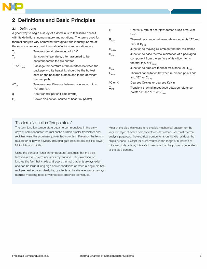
4.3. Thermally Enhanced Circuit BoardsSome commonly used techniques to improve thermal performance are

not addressed in the JEDEC51 specifications. As illustrated in Figure

6, dedicated copper islands may be placed near heat generating

components to conduct heat from the IC and to convect and radiate

heat from the PCB’s surface. Also, designers may attach a heatsink to

the backside of the PCB or even the top of the package. PCB traces

that conduct high current to power devices are commonly made as

large as allowable so as to minimize ohmic heating and enhance heat

flow. Heat generating devices are sometimes placed near other cooler

components, such as connectors, transformers or capacitors,

to improve dispersion. Modules designed for high power may very well

have heavy copper cladding with vias to the back of the board or to

internal copper planes. These measures and others can yield thermal

resistances substantially lower than those obtained from the JEDEC

specified tests.

The board illustrated in Figure 6 shows how a PCB might be modified

to reduce thermal impedance. To help users optimize thermal layouts,

many manufacturers specify thermal resistance with such thermally

enhanced boards. These ratings usually include a curve of thermal

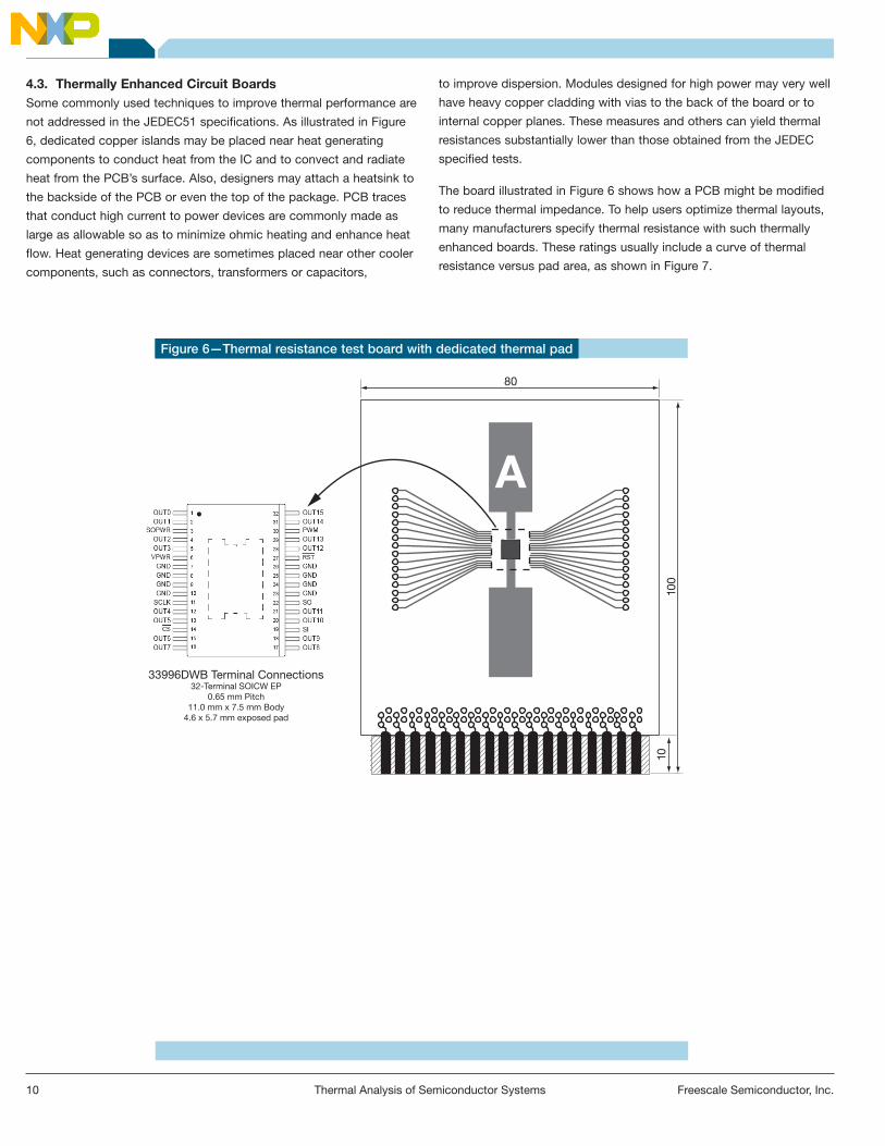
resistance versus pad area, as shown in Figure 7.

Figure 6—Thermal resistance test board with dedicated thermal pad

A

33996DWB Terminal Connections32-Terminal SOICW EP

0.65 mm Pitch11.0 mm x 7.5 mm Body

4.6 x 5.7 mm exposed pad

80

100

10


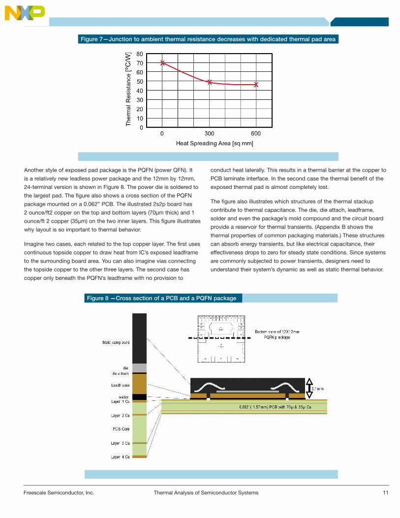
Another style of exposed pad package is the PQFN (power QFN). It

is a relatively new leadless power package and the 12mm by 12mm,

24-terminal version is shown in Figure 8. The power die is soldered to

the largest pad. The figure also shows a cross section of the PQFN

package mounted on a 0.062” PCB. The illustrated 2s2p board has

2 ounce/ft2 copper on the top and bottom layers (70µm thick) and 1

ounce/ft 2 copper (35µm) on the two inner layers. This figure illustrates

why layout is so important to thermal behavior.

Imagine two cases, each related to the top copper layer. The first uses

continuous topside copper to draw heat from IC’s exposed leadframe

to the surrounding board area. You can also imagine vias connecting

the topside copper to the other three layers. The second case has

copper only beneath the PQFN’s leadframe with no provision to

conduct heat laterally. This results in a thermal barrier at the copper to

PCB laminate interface. In the second case the thermal benefit of the

exposed thermal pad is almost completely lost.

The figure also illustrates which structures of the thermal stackup

contribute to thermal capacitance. The die, die attach, leadframe,

solder and even the package’s mold compound and the circuit board

provide a reservoir for thermal transients. (Appendix B shows the

thermal properties of common packaging materials.) These structures

can absorb energy transients, but like electrical capacitance, their

effectiveness drops to zero for steady state conditions. Since systems

are commonly subjected to power transients, designers need to

understand their system’s dynamic as well as static thermal behavior.

Figure 7—Junction to ambient thermal resistance decreases with dedicated thermal pad area

Figure 8 —Cross section of a PCB and a PQFN package


4.4. Transient Thermal Response RatingsIn many systems the worst case conditions occur during a transient

condition, such as when inrush current flows into a cold lamp filament,

startup or stall currents appear in a motor or a short circuit causes fault

current. The duration of such a transient could very well be far shorter

than the system’s thermal time constant, especially since we often

use intelligent power devices to manage such events. If the system is

designed to meet worst case transient conditions for an unnecessarily

long time, the system will be over designed. Knowing how the system

responds to thermal transients helps the designer size components

and provide adequate, but not unnecessary, heatsinking.

When you include characterization in the time domain to the many

possible ways to characterize a device in steady state, the possible

options are too large to manage. To provide the most universally

useful data, the industry has adopted and promoted a concept called

“transient thermal response.”

Transient thermal response is a device’s or a system’s thermal

response to a step input of power. Note that the step input starts at

zero power, steps to some amplitude, then remains at that amplitude

forever. A transient thermal response curve is a plot of the junction

temperature rise as a function of time. As such, the curve incorporates

the thermal effects of a device’s entire structure. Manufacturers usually

create these curves empirically, but they can create them with models

as well.

Each point on the curve shows the die’s maximum temperature versus

how long the power pulse has been present. Transient response curves

can be referenced to case or ambient temperature.

It is important to note that the specific shape of the power pulse used

in the characterization may not match the shape of the pulse of interest

in the application. Therefore, it is important to remember what the

thermal response curves represent and to use them accordingly.

Figure 9 shows the transient thermal response curve of a transistor in a

28-pin SOIC. The far right side of the curve shows the device’s steady

state thermal resistance. In this case the three possible values are for

variously sized thermal pads.

Figure 9—Transient thermal response curve

0.001 0.01 0.1 1.0 10 100 1000

1.0

10

100

0.1

Single Pulse Width, tp (seconds)

Z JC

[K /W]

TJ initial

TJ peak

Pulse Width

PD

Minimum footprint A = 300mm 2

A = 600mm 2

Transient Thermal Response [C/W]


At narrow pulse widths the thermal impedance is far less than its

steady state value. For example, at one millisecond (ms) the thermal

impedance is only 0.2ºC/W, about 100 times less than the steady state

RQJA value.

Near the center of the graph the three curves diverge, implying that

for transients of less than one or two seconds in duration the device’s

heatsinking does not affect the peak temperature. Of course, this

is true because the heat wave front begins to exit the package after

those narrow pulse durations.

Part of the beauty of the transient thermal response curves is their

ease of use. Replacing RQJA with Z

QJA in the basic thermal equation we

get:

TJpk = TA + (PD ZQJA) (Eq. 8)

Now let’s assume that a system experiences a power transient with the

following characteristics and ambient temperature:

Power pulse width, tp = 1ms

PD = 50W

TA = 75ºC

From Figure 9 we can estimate ZQJA for a 1ms pulse width:

ZQJA @ 1ms = 0.2ºC/W

then,

ΔTJApk = (TJpk – TA) = PD ZQJA

TJpk = TA + (PD ZQJA)

TJpk = 75ºC + (50W * 0.2ºC/W)

TJpk = 75ºC + 10ºC

TJpk = 85ºC

To clarify understanding further and illustrate the importance of using

such curves properly, consider the initial junction temperature of this

example. It was not explicitly defined, but the use of the method sets

its value. Transient response curves apply only to systems that have

no initial power dissipation and that are thermally at equilibrium at time

zero. Therefore, in this example the initial junction temperature must be

the ambient temperature, or 75ºC.

Clever ways have been devised to use the transient response curves

for repetitive pulses of the same magnitude, alternate pulse shapes

and pulse trains of varying pulse widths and magnitudes. The basic

concept used to achieve the broader usage is the “Superposition

Principle.” This principle states that for linear systems the net effect

of several phenomena can be found by summing the individual effects

of the several phenomena. References 1, 2 and 8 explain these

techniques in detail.

5 Ramifications of High Operating TemperatureMotivation to conduct thermal assessments arises from an

understanding of how high operating temperature affects circuit

assemblies and their reliability. Some of the effects are well known;

others are much more subtle. Only a few can be briefly

mentioned here.

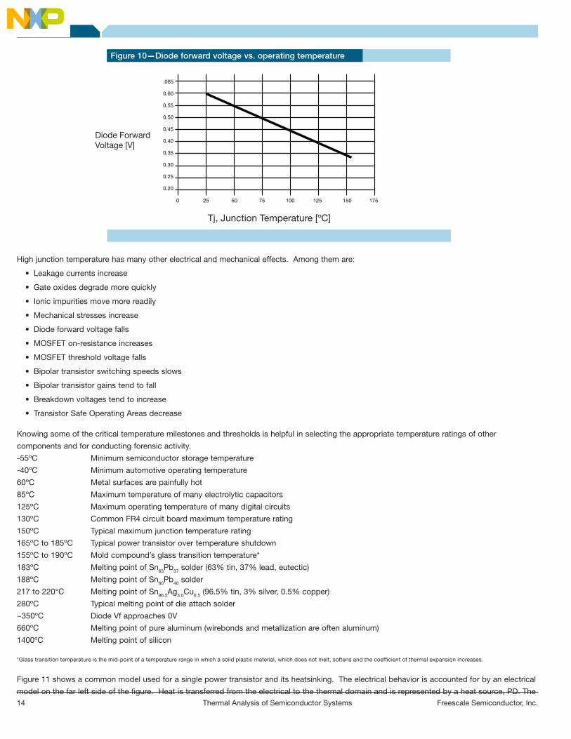
One interesting effect relates to all P-N junctions on a die. A graph

of diode forward voltage, Vf, as a function of temperature is shown

in Figure 10. It contains no surprises, showing the well-known and

well-behaved decrease in diode forward voltage with increasing

temperature. Extrapolating the curve to an even higher temperature

reveals that the forward voltage approaches 0V at about 325ºC.

The same relationship applies to the base-emitter junctions of a

device’s bipolar transistors, whether they are parasitic or not. The

result is that at a very high temperature even modest base-emitter

voltage can begin to turn on a transistor even though its base drive

circuit is trying to keep the BJT off. A similar phenomenon occurs

with MOSFETs because their gate-source threshold voltages fall with

temperature. Consequently, if a severe electrical transient generates a

hotspot, a BJT or MOSFET could reach a point of uncontrolled turn on.

Its temperature may continue to increase, and permanent damage

may ensue.


High junction temperature has many other electrical and mechanical effects. Among them are:

• Leakagecurrentsincrease

• Gateoxidesdegrademorequickly

• Ionicimpuritiesmovemorereadily

• Mechanicalstressesincrease

• Diodeforwardvoltagefalls

• MOSFETon-resistanceincreases

• MOSFETthresholdvoltagefalls

• Bipolartransistorswitchingspeedsslows

• Bipolartransistorgainstendtofall

• Breakdownvoltagestendtoincrease

• TransistorSafeOperatingAreasdecrease

Knowing some of the critical temperature milestones and thresholds is helpful in selecting the appropriate temperature ratings of other

components and for conducting forensic activity.

-55ºC Minimum semiconductor storage temperature

-40ºC Minimum automotive operating temperature

60ºC Metal surfaces are painfully hot

85ºC Maximum temperature of many electrolytic capacitors

125ºC Maximum operating temperature of many digital circuits

130ºC Common FR4 circuit board maximum temperature rating

150ºC Typical maximum junction temperature rating

165ºC to 185ºC Typical power transistor over temperature shutdown

155ºC to 190ºC Mold compound’s glass transition temperature*

183ºC Melting point of Sn63Pb37 solder (63% tin, 37% lead, eutectic)

188ºC Melting point of Sn60Pb40 solder

217 to 220°C Melting point of Sn96.5Ag3.0Cu0.5 (96.5% tin, 3% silver, 0.5% copper)

280ºC Typical melting point of die attach solder

~350ºC Diode Vf approaches 0V

660ºC Melting point of pure aluminum (wirebonds and metallization are often aluminum)

1400ºC Melting point of silicon

*Glass transition temperature is the mid-point of a temperature range in which a solid plastic material, which does not melt, softens and the coefficient of thermal expansion increases.

Figure 11 shows a common model used for a single power transistor and its heatsinking. The electrical behavior is accounted for by an electrical

model on the far left side of the figure. Heat is transferred from the electrical to the thermal domain and is represented by a heat source, PD. The

Figure 10—Diode forward voltage vs. operating temperature

.065

0.60

0.55

0.50

0.45

0.40

0.35

0.30

0.25

0.20

Tj, Junction Temperature [ºC]

0 25 50 75 100 125 150 175

Diode Forward Voltage [V]


symbol for the electrical current source is reused in the thermal domain

to denote the through variable. The heat source feeds successive RC

networks that model the behavior of the actual mechanical assembly.

Figure 11 shows three RC pairs, but a larger number could be used

to more accurately model a complex system, or a smaller number

could be used for a simple thermal network. The values of the R’s

and C’s can be estimated using the system’s material properties and

physical dimensions, or they can be extracted from empirical tests.

For example, when the system is powered and is in steady state, the

thermal resistances can easily be derived from the power dissipation

and the temperatures at the three thermal nodes. Characterizing the

transient response requires monitoring temperature response to a step

input of power.

A good engineer will want to consider several aspects of this

representation. First is the meaning of the reference, or ground,

connection in the thermal domain. Since it is a node within the

thermal domain, it is an across variable and must represent some

reference temperature. There are two natural choices for this reference

temperature: ambient temperature or absolute zero. A simple

representation is to use absolute zero as the reference temperature

then use a temperature source for ambient temperature.

The second consideration is how to terminate the thermal

capacitances. The representation in Figure 11 connects the capacitor

to the reference terminal. However, a circuit with an equivalent thermal

response can be created with each of the capacitors in parallel with

their respective thermal resistors. Some tools used to extract the RC

thermal “ladder” more readily provide a circuit with the capacitors

in parallel with the resistors. Either capacitor arrangement suffices if

the capacitor values are selected accordingly. The disadvantage of

the parallel RC configuration is that the capacitance values do not

directly relate to the system’s physical features, that is, they cannot be

calculated from the material’s density, capacity and volume.

The model shown in Figure 11 is of a single transistor and

consequently lacks any provision for thermal coupling between

neighboring components. For circuits with multiple power dissipating

elements the components in Figure 11 are replicated for each heat

generating device, and thermal coupling resistors are placed between

each combination of nodes. Obviously, the thermal schematic

becomes more complex, but perhaps worse, the values of the new

components must be determined, most commonly through empirical

testing.

The thermal circuit shown in Figure 12 is a popular way of roughly

assessing multiple device behavior within a module. This method is not

used for transient conditions, so Figure 12 does not include thermal

capacitors. Each power dissipating device is treated independently of

the others and is assigned a junction to ambient thermal resistance

based on datasheet characterization and allotted circuit board area.

The designer estimates the module’s internal air temperature rise

above ambient based on experience and adjusted to account for

the module’s size and its other thermally significant features. Finally,

device junction temperatures are estimated from the device’s RQJA, its

power dissipation and the module’s internal air temperature, which is

the “ambient” temperature for the power device.

This method has the following three key weaknesses:

Figure 11—Electrical and Thermal Domain Circuits

6 Thermal Circuits

Rthj-cPd

Tjunction

Cthj-c

Rthc-hs

Cthc-hs

Rthhs-a

Cthhs-a AmbientTemperature

TcasePowerTransistor

Theatsink

ThermalDomain

ElectricalDomain

Device Device toHeatsink

Heatsink toAmbient


1. It does not account for thermal coupling between devices on the

PCB. For this method devices affect one another only through their

effect on the internal ambient temperature.

2. It assumes a constant internal air temperature even though we

know “ambient” temperature within a module varies substantially

with distance from the heat sources. Figure 13 illustrates the

difficulty of selecting a single value for internal “ambient”

temperature.

3. Conditions existing in a module differ considerably from the

conditions used to specify the rated junction to ambient thermal

resistance. The PCB’s thermal characteristics differ and module’s

small volume constricts the flow of convective currents.

In spite of its clear drawbacks, this method is popular because it

quickly yields a rough estimate of operating temperature.

Other approaches are used, but all have limitations because each

inherently attempts to simplify a complex thermal circuit using a few

Figure 12—Popular thermal model for a module with multiple power devices

Figure 13—Thermal gradients within a module.

Module Housing

Power Gene rating Devices

internal “ ambient” tempe rature

Ta = 85ºC


lumped components. One alternate approach accounts for thermal

coupling between devices and is practical for systems with up to four

or five power devices. The improved accuracy comes at the cost of

additional empirical characterization and the need to solve several

or even many simultaneous equations. As the number of power

components increases, this rapidly becomes more difficult.

The first step of this method is to measure the junction to ambient

thermal resistance of each device when all other devices are not

generating power. Such a direct measurement gives the designer

an accurate value for the thermal resistance of that device in that

application. As a check, the calculated value should be compared to

the thermal resistance specifications.

The next step is to determine how each device heats its neighbors,

that is, the thermal coupling coefficients between devices. Use either

a thermal mock-up or a module prototype to determine these thermal

coupling factors. You can determine the coupling factors by powering

only a single device and measuring the temperature rise at every other

critical device. The coupling coefficient is the ratio of the induced

temperature rise in the unpowered device and temperature rise in the

powered device caused by self heating.

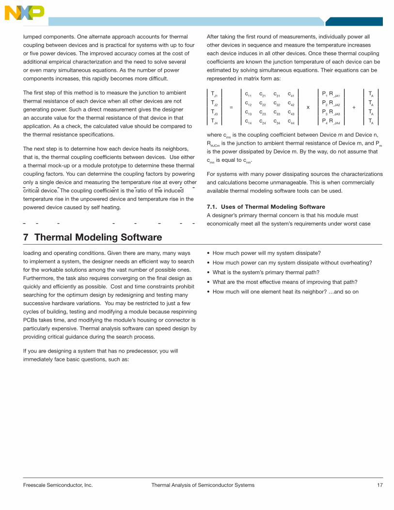
After taking the first round of measurements, individually power all

other devices in sequence and measure the temperature increases

each device induces in all other devices. Once these thermal coupling

coefficients are known the junction temperature of each device can be

estimated by solving simultaneous equations. Their equations can be

represented in matrix form as:

TJ1

=

c11 c21 c31 c41

x

P1 R_JA1

+

TA

TJ2 c12 c22 c32 c42 P2 R_JA2 TA

TJ3 c13 c23 c33 c43 P3 R_JA3 TA

TJ4 c14 c24 c34 c44 P4 R_JA4 TA

where cmn is the coupling coefficient between Device m and Device n,

RQJCm is the junction to ambient thermal resistance of Device m, and Pm

is the power dissipated by Device m. By the way, do not assume that

cmn is equal to cnm.

For systems with many power dissipating sources the characterizations

and calculations become unmanageable. This is when commercially

available thermal modeling software tools can be used.

7.1. Uses of Thermal Modeling SoftwareA designer’s primary thermal concern is that his module must

economically meet all the system’s requirements under worst case

7 Thermal Modeling Softwareloading and operating conditions. Given there are many, many ways

to implement a system, the designer needs an efficient way to search

for the workable solutions among the vast number of possible ones.

Furthermore, the task also requires converging on the final design as

quickly and efficiently as possible. Cost and time constraints prohibit

searching for the optimum design by redesigning and testing many

successive hardware variations. You may be restricted to just a few

cycles of building, testing and modifying a module because respinning

PCBs takes time, and modifying the module’s housing or connector is

particularly expensive. Thermal analysis software can speed design by

providing critical guidance during the search process.

If you are designing a system that has no predecessor, you will

immediately face basic questions, such as:

• Howmuchpowerwillmysystemdissipate?

• Howmuchpowercanmysystemdissipatewithoutoverheating?

• Whatisthesystem’sprimarythermalpath?

• Whatarethemosteffectivemeansofimprovingthatpath?

• Howmuchwilloneelementheatitsneighbor?…andsoon


Three analysis tools can be used in combination to answer these and

other questions:

1. Analysis using manufacturers’ thermal ratings and characterizations

2. Empirical testing of a prototype or of a thermal mock-up

3. Thermal modeling

Before using a set of thermal modeling tools, it’s appropriate to

consider the purpose of the modeling, the characterization data

available to support those models and what a particular software tool

can and cannot provide. These are some of the best uses of thermal

analysis software:

Provide tradeoff assessments before any hardware is built A model of a proposed implementation is a fast and low-cost way of

assessing if that implementation can potentially meet the system’s

requirements. However, you should expect that a first pass thermal

model will likely require refinements or even major revisions after you

compare the model’s simulation results to empirical test results of

actual hardware.

Uncover poorly understood thermal phenomenaAfter you decide on the first pass hardware, based on an initial thermal

model, the next steps are to build the hardware, characterize it and

compare empirical test results to the model’s predictions. Implicit in

this discovery process is that the designer must calibrate and validate

the model by empirically testing hardware.

More than likely there will be mismatches between the empirical and

modeled results. These incongruities identify thermal behaviors that

were not modeled properly, most likely because they were poorly

understood, thought to be unimportant or simply overlooked. Perhaps

the best use of modeling is to identify critical module characteristics

that were misrepresented in the model and to use that information to

improve your understanding of the module.

A calibrated thermal model speeds developmentOnce a thermal model is calibrated it becomes a powerful tool to

explore potential variations in the next layout iteration. Altering the

model and rerunning simulations is usually much faster and less

expensive than modifying the layout and retesting the hardware.

Once you create a validated thermal model it can, of course, be used

as a starting point for future modules of similar design.

A model can be used to assess test conditions that are difficult to createTesting a module under some conditions is difficult or impractical. In

these cases a calibrated thermal model can be used instead.

Testing under worst case conditions is a good example of a set of

system conditions that are difficult to create. Let’s assume that you

would like to test the system with power transistors that have worst

case on resistances. You are not likely to find such devices for

empirical testing, but modifying the transistor’s power dissipation in the

model is easy. Or, you may have hardware limitations, such as oven

volume or temperature range, that prohibit certain tests. These could

be explored in the simulated domain instead.

Thermal models accurately simulate behavior of simple structures A thermal model of a simple structure can be quite accurate because

we can precisely describe simple structures mathematically. This

strength of thermal modeling gives it a special advantage for simple

structures that are difficult to empirically test, such as a power die

on a leadframe. Empirical testing is not likely to help map junction

temperature variations across a die, especially during transients. A

calibrated model is a handy tool for these situations.

Thermal models provide a means to estimate a system’s response to power transients A system’s worst case operating conditions are often transient, so

dynamic conditions often dictate the system’s required capability. It’s

difficult enough to envision how heat flows in a system under steady

state conditions let alone estimating how temperatures change during

a transient condition. Models can provide badly needed guidance in

these situations. Some allow you to create movies of the temperature

during transients, providing the designer with a more intuitive sense of

how the system is performing.


7.2. Thermal Modeling Software OptionsThere are quite a few commercially available thermal modeling software

packages. Each package claims its niche. Whether you are selecting

a package or using one that your company already has, it is good to

understand how they differ. Some of the differentiating features are:

• Cost,includinghardwareandmaintenancefees

• Simulationspeed

• Trainingrequiredforcompetency

• Abilitytomodelallthreemodesofheattransfer,whichfor

convection requires the ability to model fluid flow

• Abilitytomodelresponsestotimevaryingpowerwaveforms

• AbilitytoimportfilesfromotherCADpackages

• Methodofmanagingboundaryconditions

• Abilitytouseamulti-levelnestedmesh

• Abilitytolinkthermalmodelstomodelsinotherdomains(e.g.,

electrical models)

• Inclusionofasoftwarelibrarythatcontainscommonthermal

elements, such as heatsinks, enclosures, PCBs, etc.

• Abilitytoviewandexportasimulation’sresults

• Customersupport,includingtechnicalliterature

• Numericalmethodusedtosolvethegoverning

mathematical equations

A program’s numerical method, the last item in the above list, is the

most fundamental feature of each program. The numerical method is

the means by which the software resolves the governing

mathematical equations.

Numerical methods used in thermal analysis software include the

Boundary Element Method, Finite Difference Method, Finite Element

Method and Finite Volume Method. The latter is the method most often

used in computational fluid dynamics (CFD) software.

The particular numerical method a program uses makes it more or

less suitable for specific modeling tasks. The most obvious example

is CFD software. Like all viable thermal analysis software, it accounts

for conduction and radiation. But CFD also predicts fluid flow, which

is necessary to model convection. Therefore, if convection is a primary

transport method in your systems, you will likely require CFD software.

ANSYS is one well known CFD thermal analysis software supplier that

offers CFX, Fluent, Iceboard and Icepak. Flomerics is another well

respected vendor and provides Flowtherm, which is the simulation

software used to create the image in Figure 13. CFD programs provide

the ability to view and export images of fluid speed and direction. This

feature helps to clearly illustrate the size and effectiveness of thermal

plumes, which are likely to form above hot surfaces.

When convection is not a significant thermal transport mechanism, a

program capable of modeling fluid flow is not necessary. An example

of such a system is a semiconductor package mounted to a heatsink

that is at a fixed or known temperature. A software package optimized

for conductivity might simulate faster or give more accurate results,

such as one using the Boundary Element Method. Instead of breaking

the modeled volume into a mesh of much smaller units, the BEM

creates a mesh on the surface of a solid. From the conditions at the

surface, it predicts the temperature and heat flux within the solid.

Because the BEM does not discretize the volume, it does not suffer

from the problems associated with having a mesh size that is too small

(excessively long simulation times) or too large (reduced accuracy). For

simple structures, such as a die in a package, the BEM is a fast and

accurate numerical method. Freescale engineers have successfully

used Rebeca 3D, a BEM package supplied by Epsilon Ingénierie, to

evaluate hotspot temperature of power die in a multi-die package.

Even the most sophisticated thermal analysis software package is

not a panacea. Obviously, the quality of its predictions depends on

the model’s inputs, such as the system’s physical dimensions and

material properties. The results also improve with the detail included

in the model, but the simulation times increase accordingly. Therefore,

regardless of which modeling software is used, to obtain the most

value from a simulation you should carefully discuss the system’s

pertinent features with the engineer creating the model, including: the

mechanical features of the system; heat source sizes and locations;

potential thermal paths; all material characteristics; system orientation;

physical boundary to be modeled, etc. The engineer creating the

model should carefully explain the simplifying assumptions he/she

plans to make.

Appendix B contains a table of thermal properties of materials used in

typical semiconductor packages.


The tools used for empirical thermal analysis are fairly well known.

The most common tool, of course, is the thermocouple. A few

guidelines to their use are:

1. Make sure your thermocouple type (J, K, T or E) matches your

meter setting.

2. Use small gauge thermocouple wires. This reduces the heatsinking

effect the leads have on the device under test.

3. Monitor as many points as practical to improve your overall

understanding of the circuit and to enhance your chance of

detecting unexpected hot spots.

4. Place probes at nodes as close as practical to the die of interest.

This measurement location need not be in the primary thermal

path. For instance, the temperature at the top of the package or

at an exposed tab may be very close to the die temperature even

though the measurement location is not in the primary

thermal path.

Infrared scanning is a very helpful technique because it provides

information about the entire scanned area. Discovering unexpected

hot spots, such as undersized PCB traces or connector pins, with

an infrared scan is not uncommon. This can be very helpful during

prototyping where assembly problems might otherwise go unnoticed. A

disadvantage of thermal imaging is that the camera must have access

to the device or PCB under test. Opening a module to provide such

access significantly alters the behavior you are trying to measure.

Handheld, infrared, contactless thermometers are inexpensive and

easy-to-use tools for taking spot measurements.

It’s possible to measure a device’s junction temperature by monitoring

a temperature sensitive parameter (TSP) of one of its components. A

diode’s forward voltage, Vf, is one the most commonly used TSPs, and

diodes may be readily accessible as ESD structures on a logic pin, for

example. The body diode of a power MOSFET is another often used

component, but using that diode requires reversing the current in the

MOSFET, which requires a bit of circuit gymnastics. Over temperature

shutdown (if available), MOSFET on-resistance and MOSFET

breakdown voltage are also options. Using a TSP requires establishing

the TSP’s variation over temperature, which must be done at near

zero power.

When making thermal resistance measurements, you should try to

use power levels that will generate easily measurable temperature

increases. A larger junction to ambient temperature differential

increases the quantity you are attempting to measure (temperature rise)

relative to any potential measurement errors in the system.

A common system requirement is that a module must operate at a

certain ambient temperature in still air. These conditions sound simple

enough to create, but the high test temperature will require an oven

and an oven often uses circulating air to control the temperature. Its

fan ensures the oven’s air is not still. To circumvent this problem

you can place a box in the oven and place the module in that box.

Of course, the box reduces the air speed around the module. With

this arrangement the oven temperature can be adjusted to attain the

specified “ambient” temperature in the box.

If you are designing a system that has a predecessor, use data from

that module as a starting point. If the system has no predecessor, then

consider building a thermal mock-up that will mimic the final module’s

behavior. Such a mock-up might have little or no electrical similarity

to the intended module, but it should have mechanical and thermal

similarity. Because an electrical circuit does not have to be built,

programmed and debugged, you might be able to create a thermal

prototype of your module very quickly to assess total module power

budget, thermal coupling, affects in changes to the primary thermal

path, etc.

Finally, plan to use empirical testing in conjunction with thermal

resistance ratings and thermal models to enhance your understanding

of the system.

8 Empirical Analysis Techniques


There are many ways to reduce the operating temperature of

semiconductor devices. Some of the techniques add little or no

additional cost to the module. Below are some suggestions:

Reduce the module’s or IC’s thermal load.The most direct way to deal with excessive heat is to not generate it in

the first place. Portions of the circuit may be turned off. Load shedding

(if allowed), careful fault management, using oversized power

transistors or using ICs with power saving features are some of the

ways to cut

a module’s total dissipation. Carefully defining the module’s worst case

operating conditions is sometimes the most effective way to reduce

power dissipation.

Reduce thermal impedance in the IC’s immediate vicinity. Semiconductor die are quite small compared to the size of a typical

module, and this results in very high heat flux in the die, the package

and its immediate vicinity. Therefore, thermal resistance encountered

early in the thermal path causes a large temperature gradient. That is

why temperature often falls rapidly as you move from the die into its

package and then into rest of the system. The most effective place

to focus resources to reduce thermal resistance is where the thermal

gradient is highest. So, be especially mindful of how the package is

attached to the PCB or heatsink and how thermal energy is transferred

and spread in that area. Spreading the heat at the beginning of the

thermal path not only reduces the thermal resistance near the IC, but it

also provides a broader area to further disseminate the heat. Reducing

the thermal impedance close to the die and package is mandatory for

good thermal performance.

Use a continuous low impedance path from the IC to ambient.Around the IC, provide an uninterrupted copper path to a large pad to

radiate heat, a heatsink, the module’s harness, etc. Any small break

in low impedance material is highly detrimental. Provide redundant

thermal paths where possible.

Increase the surface area from which the heat exits the module.Ultimately, some surface will radiate the module’s heat or disperse it

by convection. Use all available features, such as the harness as well

as the housing. The utility of the harness depends on the number and

gauges of its wires, its insulation, its own ohmic losses and how well

heat can flow from the PCB through the connector and into

the harness.

Separate heat generating components.Place heat generating components as far apart as possible to reduce

thermal coupling effects. The thermal gradient is high near a power

dissipating device, so even small amounts of separation help reduce

thermal coupling.

Use thick copper cladding, if allowable. The cross sectional area of a trace is quite small and can constrict

heat flow. Using heavier copper cladding reduces this effect. However,

if fine pitch ICs are used on the board, using heavier copper cladding

may violate manufacturing guidelines.

Beware of PCB trace and connector pin heating.Modern power electronics devices can have very low on-resistances.

It’s quite possible that the PCB traces and connector pins that feed

current to these devices contribute more ohmic losses to the system

than the power transistors do. Such heating may be avoidable if

traces are upsized. Reducing trace ohmic losses may be the least

expensive way to reduce the module’s total power dissipation. Trace

width calculators, which also predict trace temperature rise, are readily

available on the internet.

Consider the effects of PCB and module orientation.Heat convection is more efficient for a vertically mounted board.

Remember that components above heat producing devices run hotter

than those below.

If the board is to be horizontally mounted, place heat generating

devices on the PCB’s topside, if possible. A thermal plume forms more

readily on a board’s topside and it helps disperse heat.

9 Optimizing the Thermal Environment


Take advantage of thermal capacitance, if possible.Worst case conditions are often briefer than the module’s thermal time

constant. Upon a change in operating conditions, a module can easily

take more than 10 minutes to stabilize thermally. The system may be

able to store the energy from the worst case conditions in the module’s

thermal capacitance. Heat sinks, heavy copper and multi-layered

boards all add to the module’s thermal capacitance.

Remember, too, that even when a device is mounted to a worst case

board, the device itself has some ability to absorb energy. If a device

has fast fault detection circuitry, it may be able to absorb the energy

and manage the fault without harm to the device, the PCB or the load.

Expect surprises. Because we have a limited innate ability to sense thermal phenomena,

we lack an intuitive feel for how thermal systems behave. This makes

it advisable to monitor temperature at many points on a PCB or, better

yet, photograph the module, its PCB, and its harness with an infrared

camera. Any unexpected temperatures you find point you to aspects

of the thermal circuit that you do not completely understand. Finding

these surprises provides valuable clues that can lead to a better

understanding of the module’s thermal behavior.

10 Appendices10.1. Appendix A—List of JESD51 Series Publications

JESD51 “Methodology for the Thermal Measurement of Component Packages (Single Semiconductor Device)”

JESD51-1 “Integrated Circuit Thermal Measurement Method—Electrical Test Method (Single Semiconductor Device)”

JESD51-2 “Integrated Circuit Thermal Test Method Environmental Conditions—Natural Convection (Still Air)”

JESD51-3 “Low Effective Thermal Conductivity Test Board for Leaded Surface Mount Packages”

JESD51-4 “Thermal Test Chip Guideline (Wire Bond Type Chip)”

JESD51-5 “Extension of Thermal Test Board Standards for Packages with Direct Thermal Attachment Mechanisms”

JESD51-6 “Integrated Circuit Thermal Test Method Environmental Conditions—Forced Convection (Moving Air) ”

JESD51-7 “High Effective Thermal Conductivity Test Board for Leaded Surface Mount Packages”

JESD51-8 “Integrated Circuit Thermal Test Method Environmental Conditions—Junction-to-Board”

JESD51-9 “Test Boards for Area Array Surface Mount Package Thermal Measurements”

JESD51-10 “Test Boards for Through-Hole Perimeter Leaded Package Thermal Measurements”

JEDEC51-12 “Guidelines for Reporting and Using Electronic Package Thermal Information”

10.2. Appendix B—Thermal Properties of Common Semiconductor Packaging Materials

Material Conductivity K Relative Conductivity

Thermal Capacity CP Density Volumetric Heat

Capacity

Relative Volumetric Heat

Capacity

(W/m K) – (J/kg K) (kg/m3) (J/K m3) –

Epoxy Mold Compound 0.72 0.00200 794 2020 1603880 0.4748

Silicon (at 25C) 148 0.41111 712 2328.9 1658177 0.4908

SnPb Solder 50 0.13889 150 8500 1275000 0.3774

Silver Filled Die Attach 2.09 0.00581 714 3560 2541840 0.7524

CU Lead Frame 360 1.00000 380 8890 3378200 1.0000

FR-4 0.35 0.00097 878.6 1938 1702727 0.5040

Air 0.03 0.00008 1007 1.16 1170 0.0003

Values may vary with specific type of material, temperature


11 References1. “MC33742DW Thermal Datasheet,” Freescale Semiconductor, April 2007, http://www.freescale.com

2. “MC33996 Datasheet”, Freescale Semiconductor, June 2007, http://www.freescale.com

3. Roger Stout, “Linear Superposition Speeds Thermal Modeling”, Part 1, pp20-25, Power Electronics Technology, January 2007

4. Roger Stout, “Linear Superposition Speeds Thermal Modeling”, Part 2, pp28-33, Power Electronics Technology, February 2007

5. T. Hopkins, et al, “Designing with Thermal Impedance”, SGS-Thompson Application Note AN261/0189, reprinted from Semitherm

Proceeding 1988

6. “Understanding the JEDEC Integrated Thermal Test Standards”, Advanced Thermal Solutions, Inc., http://www.QATS.com

7. JESD51-1 through JESD51-12 specifications, JEDEC Solid State Technology Association, http://www.jedec.org

8. REBECA-3D, http://www.rebeca3d.com

9. Roehr, Bill and Bryce Shiner, “Transient Thermal Resistance - General Data and Its Use,” AN569 in Motorola Power Applications

Manual, 1990, pp. 23-38 or http://www.bychoice.com/motorolaApps.htm

10. R. Behee, “Introduction to Thermal Modeling Using SINDA/G,” Network Analysis, Inc., http://www.sinda.com

11. “Thermocouples – An Introduction”, Omega Engineering website, http://www.omega.com

12. PCB Trace Width Calculator, http://circuitcalculator.com/wordpress/2006/01/31/pcb-trace-width-calculator/

13. “Important Questions to Ask When Evaluating Thermal Analysis Software for Electronics”, Stokes Research Institute,

http://www.stokes.ie/pdf/Questionnaire.pdf

14. M. Goosey and M. Poole, “An Introduction to High Performance Laminates and the Importance of Using Chemical Processes

in PCB Fabrication”, Rohm and Haas Electronic Materials, http://electronicmaterials.rohmhaas.com

Home Page:www.freescale.com

Power Architecture Information:www.freescale.com/powerarchitecture

e-mail:[email protected]

USA/Europe or Locations Not Listed:Freescale SemiconductorTechnical Information Center, CH3701300 N. Alma School RoadChandler, Arizona [email protected]

Europe, Middle East, and Africa:Freescale Halbleiter Deutschland GmbHTechnical Information CenterSchatzbogen 781829 Muenchen, Germany+44 1296 380 456 (English)+46 8 52200080 (English)+49 89 92103 559 (German)+33 1 69 35 48 48 (French)[email protected]

Japan:Freescale Semiconductor Japan Ltd.HeadquartersARCO Tower 15F1-8-1, Shimo-Meguro, Meguro-ku,Tokyo 153-0064, Japan0120 191014+81 3 5437 [email protected]

Asia/Pacific:Freescale Semiconductor Hong Kong Ltd.Technical Information Center2 Dai King StreetTai Po Industrial Estate,Tai Po, N.T., Hong Kong+800 2666 [email protected]

For Literature Requests Only:Freescale SemiconductorLiterature Distribution CenterP.O. Box 5405Denver, Colorado 802171-800-441-2447303-675-2140Fax: [email protected]

Information in this document is provided solely to enable system and software implementers to use Freescale Semiconductor products. There are no express or implied copyright license granted hereunder to design or fabricate any integrated circuits or integrated circuits based on the information in this document.

Freescale Semiconductor reserves the right to make changes without further notice to any products herein. Freescale Semiconductor makes no warranty, representation or guarantee regarding the suitability of its products for any particular purpose, nor does Freescale Semiconductor assume any liability arising out of the application or use of any product or circuit, and specifically disclaims any and all liability, including without limitation consequential or incidental damages. “Typical” parameters which may be provided in Freescale Semiconductor data sheets and/or specifications can and do vary in different applications and actual performance may vary over time. All operating parameters, including “Typicals” must be validated for each customer application by customer’s technical experts. Freescale Semiconductor does not convey any license under its patent rights nor the rights of others. Freescale Semiconductor products are not designed, intended, or authorized for use as components in systems intended for surgical implant into the body, or other applications intended to support or sustain life, or for any other application in which the failure of the Freescale Semiconductor product could create a situation where personal injury or death may occur. Should Buyer purchase or use Freescale Semiconductor products for any such unintended or unauthorized application, Buyer shall indemnify and hold Freescale Semiconductor and its officers, employees, subsidiaries, affiliates, and distributors harmless against all claims, costs, damages, and expenses, and reasonable attorney fees arising out of, directly or indirectly, any claim of personal injury or death associated with such unintended or unauthorized use, even if such claim alleges that Freescale Semiconductor was negligent regarding the design or manufacture of the part.

How to Reach Us:

Learn More: For current information about Freescale products and documentation, please visit www.freescale.com.

Freescale and the Freescale logo are trademarks or registered trademarks of Freescale Semiconductor, Inc. in the U.S. and other countries. All other product or service names are the property of their respective owners. © Freescale Semiconductor, Inc. 2008Document Number: BASICTHERMALWP/ REV 0

Documents

Basin Principles of Thermal Analysis for Semiconductor Systems · 4 Thermal Analysis of Semiconductor Systems Freescale Semiconductor, Inc. 2.2. Basic Principles The basic principles