Lecture Notes

Basismodul Experimentalphysik

Physics of Nanostructures

Summer Term 2017

Katharina Broch

Monika Fleischer

Dieter Kolle

Frank Schreiber

Universitat Tubingen

Preface

Nanoscience has developed into a fascinating, important, dynamic, and rather broadsubject. In fact, it is not easy to find a definition of nanoscience which is universally ac-cepted, in contrast to many other branches of science. Along with that comes the obser-vation that the books published so far with titles involving some form of “nanoscience”differ very strongly in scope and level, from a more technological perspective and focuson, e.g., lithographic structures to a rather lifescience-oriented approach covering themany exciting opportunities arising from, e.g., high-resolution (physical) characteriza-tion methods in biology.

The present lecture notes are written from a more physics-related perspective andtry to systematically address the question what happens to condensed matter if itis ”constrained” in at least one direction, i.e. if the dimensions are reduced from 3D(bulk) to 2D (thin films), 1D (nanowires), 0D (quantum dots or nanoparticles), or other,possibly rather complex structures with at least one dimension in the nanometer range.Also, if the dimensions of a sample are reduced such that it consists of only a few atoms,there is an obvious natural connection to the molecular world. Indeed, an importanttrend is the merging of (classical) condensed matter with molecular materials.

Current research offers plenty of examples for areas related to nanoscience defined inthis spirit. The enormous amount of work on graphene and related 2D-materials, whichreceived a further boost by the 2010 Nobel prize in physics (Geim and Novoselov),is just one example. Others concern magnetism in reduced dimensions, also withsome connections to the Nobel prize (Grunberg and Fert, 2007), molecular magnets,the growing field of nanooptics and plasmonics, or organic and molecular electronics(relating to the Nobel prize for Heeger, MacDiarmid, and Hideki Shirakawa, 2000).Also what may be considered almost “traditional” semiconductor electronics, with allthe consumer electronics and optoelectronics determining so much of our everyday life,is essentially a form of nanoscience, for which the ultimate limits are a very fundamentalscientific question. An important role in this context is being played by the developmentof experimental tools, from lithographic methods to very targeted and specific chemicalpreparation routes of nanoparticles and complex hybrid structures to characterizationtools such as scanning probe microscopies and optical microscopy beyond the resolutionlimit (see Nobel prize for Moerner, Betzig, and Hell, 2014), to ever-improving X-raysources for nanodiffraction and more sensitive spectroscopic methods, with improvedspace and time resolution. At the same time, theoretical methods to calculate theproperties of novel materials and novel structures are improving, including in particularthe computing power - which itself is actually a result of nanotechnology!

The lecture notes are organized such that after a general introduction we first presentissues related to preparation and characterization of thin films and nanostructures.

3

4

After that, we present chapters on specific properties of these materials, i.e. electronic,mechanical, optical, and magnetic properties. We would like to stress, though, thatthe order of the individual chapters may be chosen differently in a practical lecturecourse. In our experience it works also well to first present chapters on, e.g. transportand explain the preparation and characterization later. The individual chapters areintentionally written such that they can be taught collectively in a course, but indifferent order and also independently.

The authors

Tubingen, April 2017

Contents

1 Introduction 1

1.1 What is nanoscience ? . . . . . . . . . . . . . . . . . . . . . . . . . . . 1

1.2 What is different on the nanoscale ? . . . . . . . . . . . . . . . . . . . . 1

1.3 Why is nanoscience interesting? . . . . . . . . . . . . . . . . . . . . . . 8

1.4 What are the fundamental questions in nanoscience ? . . . . . . . . . . 9

1.4.1 Implications of the existence of a surface . . . . . . . . . . . . . 10

1.4.2 Implications of reduced size on phase transitions . . . . . . . . . 10

1.5 What are the limits of nanoscience ? . . . . . . . . . . . . . . . . . . . 11

1.6 Scope and structure of these lecture notes . . . . . . . . . . . . . . . . 11

1.7 List of Original Literature . . . . . . . . . . . . . . . . . . . . . . . . . 11

Appendix 13

A.1 Density of states (DOS) as a function of dimension d for a dipsersionω(kn) . . . . . . . . . . . . . . . . . . . . . . . . . . . . . . . . . . . . . 13

5

6 CONTENTS

Chapter 1

Introduction

1.1 What is nanoscience ?

There are different definitions of nanoscience. For the purpose of these lecture notes,we shall simply include everything concerned with objects which are on the nanoscale(nm) in at least one dimension. This explicitly includes thin films, which are “nano”obviously only in one dimension, i.e. their thickness. Other examples include systemsnanostructured in some form (lithography or otherwise) in all three spatial dimensionsor nanoparticles etc.

In this context, while “nano” suggests simply the comparison with ≈ 1 nanometer, themore appropriate question defining the subject of these lecture notes is:

Does a given sample with a given shape or morphology and given dimensions (i.e. size)and a given material exhibit properties which in some form differ from the correspond-ing bulk system, i.e. the unconfined and infinitely extended system ?

This will be a key point in these lecture notes.

1.2 What is different on the nanoscale ?

Considering that what is commonly taught in many condensed matter lectures andtextbooks assumes a translationally invariant, infinitely extended crystal, it is notsurprising that if this key assumption is given up, new properties and fundamentallynew effects arise. We may try to categorize these in the following, but to some degree,they are interconnected, of course, such as the finite dimensions of a sample and thepresence of a surface or interface.

1. Broken translational symmetry at surfaces and interfaces:Lattice sites with reduced coordination number and with different bonds, lead-ing frequently to a different geometric structure (e.g., surface reconstruction orrelaxation) and a different local electronic structure, both with respect to theground state as well as to the excited state. Some of these points are at the

1

2 Chapter 1 Introduction

heart of surface science, which is less in the focus of these lecture notes, butwe shall nevertheless emphasize their importance, e.g., in the context of surfacechemistry and catalysis with significantly different reactivities of these differentlycoordinated atoms. Others have a direct impact on not only the surface, butthe behavior of the entire system, such as, e.g. the frequently enhanced magneticmoment per atom in magnetic nanoparticles.

2. Effect of reduced dimensions on the density of states (DOS):This a rather fundamental and general effect, which is found even if the electronicor geometric structure at the surface is not altered. It concerns both the electronicDOS as well as the DOS of bosonic excitations. As the calculations further belowshow, the scaling with dimensions is similar, but the physics affected by them isdifferent.

(a) Density of states for electrons in reduced dimensions:

Generally, the energy dependence of the electronic DOS is different for dif-ferent dimensions, with far-reaching consequences for essentially all physicalproperties.

Also, the assumption of quasi-continuous energy levels is not necessarilyvalid anymore. For instance, in a metallic nm-size particle the energy dif-ference ∆E between different quantum states of the conduction electrons(with wave vector k) becomes significant compared to, e.g., the thermal en-ergy or possibly the Zeeman energy in an external field; see, e.g., for thefree-electron gas (in a cube of side length L, with electron mass m):∆k = 2π/L → ∆E = (~∆k)2/2m = (h/L)2/2m ≈ 1.5 eV/L2(nm2)

(b) Density of states for phonons, magnons, or other bosonic quasi-particles inreduced dimensions:

Even if the dispersion relation is not changed, the integral over all exci-tations including Bose-Einstein statistics is changed by the dimensionality,which in turn changes the collective behavior. This can lead to entirelynew phenomena such as the absence of ordering, and in particular entirelydifferent temperature dependences. This discussion can be rather involved,such as, e.g., the work of the 2016 Nobel laureates in physics, J. MichaelKosterlitz, F. Duncan M. Haldane, and David J. Thouless, amongst others.

3. Confinement effects:A key point for nano-effects to occur is that the dimensions - or at least one - arenano-sized. This means we have to compare the size Lobject of the object underinvestigation to characteristic length scales Leffect of a given effect of interest inorder to evaluate whether or not we expect nano-size-driven effects. Generally, weexpect confinement effects for Lobject < Leffect. Note that this argument wouldstill hold even if there were no changes at the surface and no dimensionalityeffects on the DOS, i.e. even if the mechanisms explained above were for somereason not operational. Therefore, the confinement argument is an independentand additional mechanism for nano-sized objects to behave differently.

There are, of course, many different relevant length scales, so that a sample maybe “nano” for some effects and not for others. We shall mention here only a fewexamples:

1.2 What is different on the nanoscale ? 3

(a) The Fermi wavelength λF = 2π (3π2n)−1/3

with the electron density n.Note that λF ∝ n−1/3, so that it is much larger in semiconductors (∼ 100 nm)than in metals (∼ 0.1 nm).

(b) The spatial extension of a exciton (bound electron-hole pair), which is muchlarger than the lattice parameter for a Wannier-Mott exciton typical forSi or GaAs; from this perspective, one would expect confinement and thusnano-science effects to set in already well above atomic length scales.

(c) The exchange length in ferromagnets lex, which is ≈ 1 ... 100 nm dependingon the material. The comparison to the size of, e.g., a magnetic nanoparticleis important for the question whether or not the system is expected to be asingle-domain ferromagnet or possibly superparamagnetic.

Furthermore, there are a number of miscellaneous other issues, which are not easilyassigned to one of the above categories, but can nevertheless be significant. We shallmention that frequently the relative contribution of thermal fluctuations is stronger forsmaller samples, with possible impact on the dynamical properties. Likewise, also therelative contribution of defects can be higher.

A. Fraction of atoms at the surface for a nano-sized sample

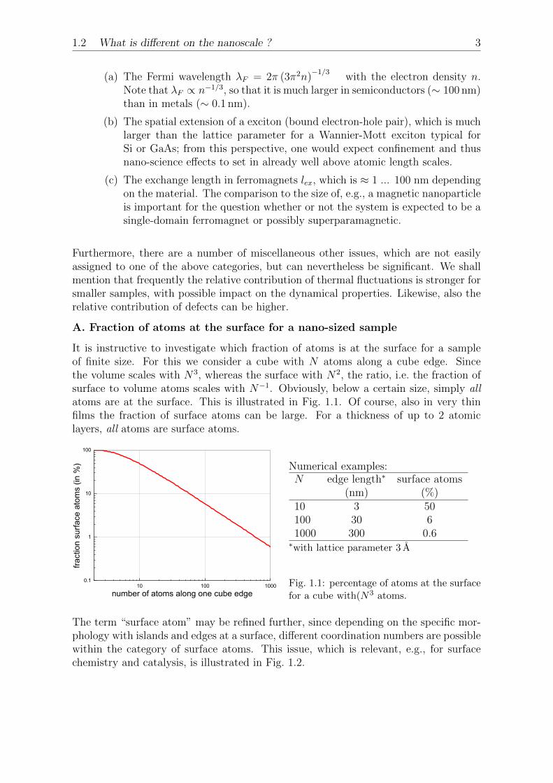
It is instructive to investigate which fraction of atoms is at the surface for a sampleof finite size. For this we consider a cube with N atoms along a cube edge. Sincethe volume scales with N3, whereas the surface with N2, the ratio, i.e. the fraction ofsurface to volume atoms scales with N−1. Obviously, below a certain size, simply allatoms are at the surface. This is illustrated in Fig. 1.1. Of course, also in very thinfilms the fraction of surface atoms can be large. For a thickness of up to 2 atomiclayers, all atoms are surface atoms.

10 100 10000.1

1

10

100

fract

ion

surfa

ce a

tom

s (in

%)

number of atoms along one cube edge

Numerical examples:N edge length∗ surface atoms

(nm) (%)10 3 50100 30 61000 300 0.6∗with lattice parameter 3 A

Fig. 1.1: percentage of atoms at the surfacefor a cube with(N3 atoms.

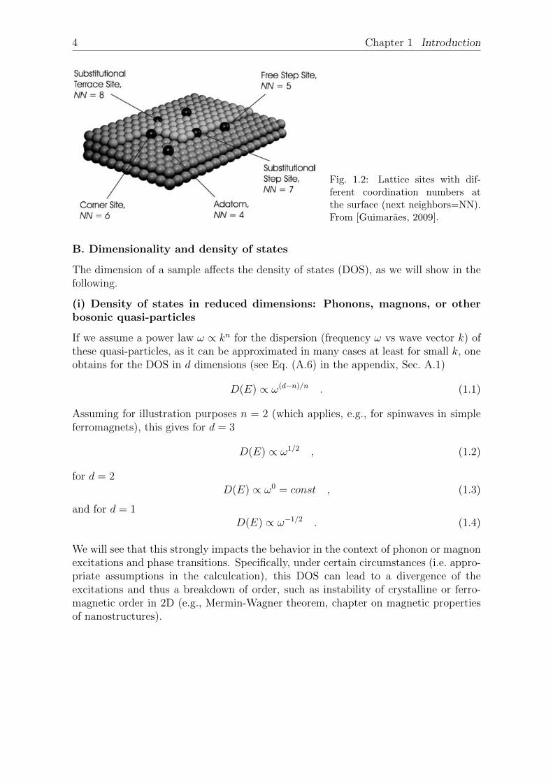
The term “surface atom” may be refined further, since depending on the specific mor-phology with islands and edges at a surface, different coordination numbers are possiblewithin the category of surface atoms. This issue, which is relevant, e.g., for surfacechemistry and catalysis, is illustrated in Fig. 1.2.

4 Chapter 1 Introduction14 1 The Basis of Nanomagnetism

Fig. 1.7. Atomic sites on a thin film showing the different coordination numbers. The numberNN of nearest neighbors of the atoms on the surface (adatom, NN = 4), atom near a step(NN = 5), atom in the step (NN = 7) and finally, a substitutional atom at the surface (NN = 8).(Reprinted with permission from [22])

the same number of nearest neighbors as in the macroscopic sample, but there, ofcourse, they will have a different neighborhood, formed of atoms A and B.

The atoms at the boundary of the sample, e.g., at the interface sample–vacuumare surrounded by a smaller number of neighbors: they may have one neighbor less,two less, and so on. These surface atoms may be at a plane surface, at the cornerof a step, or inside a step. An illustration of these different surroundings is given inFig. 1.7. The figure shows atoms on different locations of the same surface, atomswith 4, 5, 6, 7, and 8 near neighbor atoms.

In general, the electronic structure of the atoms with a smaller coordination num-ber is different from that of the atoms in the bulk. The density of states shows that thereduction in the coordination number results in a narrowing of the electronic bands(e.g., [5]). This effect is illustrated in Fig. 1.8, with densities of states of bulk metalscompared to those of atoms on a (100) surface. For Fe, Co, and Ni, the (100) surfaceatoms exhibit narrower density of states curves, compared to those of bulk samplesof the same materials.

The increasing orbital contribution to the magnetic moment with decreasing di-mensionality is made evident from measurements made on Co in Pt, as illustrated onTable 1.4; the increase in anisotropy energy is also apparent.

The atoms located on the interfaces also have the point symmetry at their sitesreduced, an effect that leads to level splitting and modification of the magnitude ofthe atomic magnetic moments. In Fe thin films in contact with Cu, Pd, and Ag, forexample, the Fe atoms exhibit enhanced magnetic moments (e.g., [24]).

The magnetic properties of atoms in interfaces are also affected by the presenceof defects and impurities, such as adsorbates; strain may also change these properties,and modify the lattice parameters.

Fig. 1.2: Lattice sites with dif-ferent coordination numbers atthe surface (next neighbors=NN).From [Guimaraes, 2009].

B. Dimensionality and density of states

The dimension of a sample affects the density of states (DOS), as we will show in thefollowing.

(i) Density of states in reduced dimensions: Phonons, magnons, or otherbosonic quasi-particles

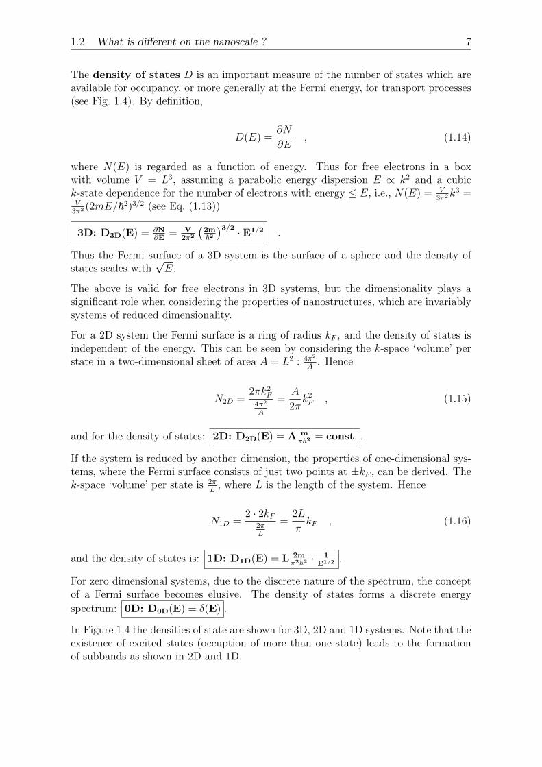
If we assume a power law ω ∝ kn for the dispersion (frequency ω vs wave vector k) ofthese quasi-particles, as it can be approximated in many cases at least for small k, oneobtains for the DOS in d dimensions (see Eq. (A.6) in the appendix, Sec. A.1)

D(E) ∝ ω(d−n)/n . (1.1)

Assuming for illustration purposes n = 2 (which applies, e.g., for spinwaves in simpleferromagnets), this gives for d = 3

D(E) ∝ ω1/2 , (1.2)

for d = 2D(E) ∝ ω0 = const , (1.3)

and for d = 1D(E) ∝ ω−1/2 . (1.4)

We will see that this strongly impacts the behavior in the context of phonon or magnonexcitations and phase transitions. Specifically, under certain circumstances (i.e. appro-priate assumptions in the calculcation), this DOS can lead to a divergence of theexcitations and thus a breakdown of order, such as instability of crystalline or ferro-magnetic order in 2D (e.g., Mermin-Wagner theorem, chapter on magnetic propertiesof nanostructures).

1.2 What is different on the nanoscale ? 5

(ii) Density of states in reduced dimensions: Electrons

Similar to bosonic quasi-particles, also the density of states as a function of energyD(E)for the free electron gas changes fundamentally upon reduction of the dimensionality orthe size of the sample (see the chapter on electronic properties of nanostructures or thecalculation below). Since many physical properties of condensed matter are directlyrelated toD(E), such as the Pauli magnetic susceptibility, the electronic contribution tothe specific heat, etc., we reproduce the explicit calculation also for electrons, althoughthe arguments (and also the power laws) for the DOS itself are the same as above forbosons, assuming n = 2, i.e. the quadratic dispersion of free electrons. Obviously, forresulting statistical mechanics calculations eventually the different quantum statisticswould enter, thus breaking the analogy for observables.

We consider (quasi-)free electrons. Although the influence of a periodic potential incrystalline materials and the resulting band-structure forms the basis for an under-standing of the electronic properties, we can often neglect the details of such band-structures, and indeed any anisotropy of the relevant band-structure, by using an ap-propriate effective mass (and still locally an approximately quadratic dispersion).

For non-interacting fermions (electrons) – ignoring Coulomb interactions by assumingscreening within the neutral crystal – confined within a volume given by the spatialextent of the confining crystal, the Hamiltonian is given by

HΨ = − ~2

2m∇2Ψ(r) = EΨ(r) , (1.5)

under the constraint that the electrons are confined to a box, which for simplicity isassumed to be a cube of side length L and volume V = L3.

The obvious boundary condition is Ψ = 0 ∀ r ∈ ∂V , but is often considered unsatis-factory since the solutions are standing waves, and electronic transport is more easilyconsidered with eigenstates which are travelling waves. It is therefore more convenientto use the so-called Born-von Karman boundary conditions

Ψ(x+ L, y, z) = Ψ(x, y, z) (1.6)

Ψ(x, y + L, z) = Ψ(x, y, z) (1.7)

Ψ(x, y, z + L) = Ψ(x, y, z) (1.8)

to remove the surface. For the solution to be confined within the box, appropriatenormalisation is required. The solution

Ψk(r) =1√V

exp(ik · r) (1.9)

is already normalised to a volume V and is characterised by the quantum number k.The energy eigenvalue is

E(k) =~2k2

2m(k = |k|) . (1.10)

6 Chapter 1 Introduction

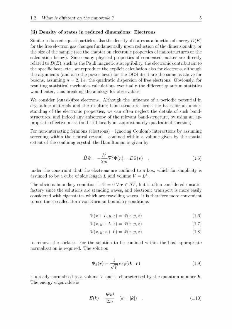
Fig. 1.3: The allowed k-states areequally spaced in all 3 directions,and the volume per state is (8π

3

V ).

With the quantum number k, Ψk(r) is also an eigenstate of the momentum operatorp = ~

i∇r and pΨ = ~kΨ, thus all eigenstates have a well-defined momentum p = ~k

or velocity v = ~k/m. The only constraint upon the allowed values of k is given bythe above boundary conditions:

eikxL = eikyL = eikzL = 1 (k = (kx, ky, kz)) . (1.11)

The allowed values of k are given by

kx =2πnxL

; ky =2πnyL

; kz =2πnzL

(nx, ny, nzinteger) (1.12)

The allowed k-states are equally spaced in all 3 directions, and the volume per state is(8π

3

V) (see Fig. 1.3). The result (8π

3

V) holds also for Lx 6= Ly 6= Lz where the spacing of

the k-states is no longer equidistant.

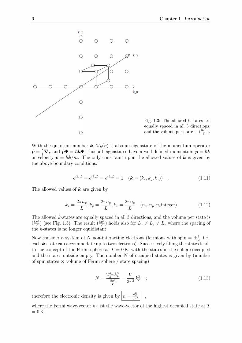
Now consider a system of N non-interacting electrons (fermions with spin = ±12, i.e.,

each k-state can accommodate up to two electrons). Successively filling the states leadsto the concept of the Fermi sphere at T = 0 K, with the states in the sphere occupiedand the states outside empty. The number N of occupied states is given by (numberof spin states × volume of Fermi sphere / state spacing)

N =243πk3F8π3

V

=V

3π2k3F ; (1.13)

therefore the electronic density is given by n =k3F3π2 ,

where the Fermi wave-vector kF ist the wave-vector of the highest occupied state at T= 0 K.

1.2 What is different on the nanoscale ? 7

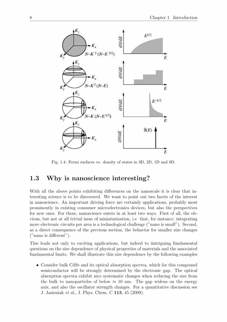
The density of states D is an important measure of the number of states which areavailable for occupancy, or more generally at the Fermi energy, for transport processes(see Fig. 1.4). By definition,

D(E) =∂N

∂E, (1.14)

where N(E) is regarded as a function of energy. Thus for free electrons in a boxwith volume V = L3, assuming a parabolic energy dispersion E ∝ k2 and a cubick-state dependence for the number of electrons with energy ≤ E, i.e., N(E) = V

3π2k3 =

V3π2 (2mE/~2)3/2 (see Eq. (1.13))

3D: D3D(E) = ∂N∂E

= V2π2

(2m~2)3/2 · E1/2 .

Thus the Fermi surface of a 3D system is the surface of a sphere and the density ofstates scales with

√E.

The above is valid for free electrons in 3D systems, but the dimensionality plays asignificant role when considering the properties of nanostructures, which are invariablysystems of reduced dimensionality.

For a 2D system the Fermi surface is a ring of radius kF , and the density of states isindependent of the energy. This can be seen by considering the k-space ‘volume’ perstate in a two-dimensional sheet of area A = L2 : 4π2

A. Hence

N2D =2πk2F4π2

A

=A

2πk2F , (1.15)

and for the density of states: 2D: D2D(E) = A mπ~2 = const. .

If the system is reduced by another dimension, the properties of one-dimensional sys-tems, where the Fermi surface consists of just two points at ±kF , can be derived. Thek-space ‘volume’ per state is 2π

L, where L is the length of the system. Hence

N1D =2 · 2kF

2πL

=2L

πkF , (1.16)

and the density of states is: 1D: D1D(E) = L 2mπ2~2 ·

1E1/2 .

For zero dimensional systems, due to the discrete nature of the spectrum, the conceptof a Fermi surface becomes elusive. The density of states forms a discrete energy

spectrum: 0D: D0D(E) = δ(E) .

In Figure 1.4 the densities of state are shown for 3D, 2D and 1D systems. Note that theexistence of excited states (occuption of more than one state) leads to the formationof subbands as shown in 2D and 1D.

8 Chapter 1 Introduction

Fig. 1.4: Fermi surfaces vs. density of states in 3D, 2D, 1D and 0D.

1.3 Why is nanoscience interesting?

With all the above points exhibiting differences on the nanoscale it is clear that in-teresting science is to be discovered. We want to point out two facets of the interestin nanoscience. An important driving force are certainly applications, probably mostprominently in existing consumer microelectronics devices, but also the perspectivesfor new ones. For these, nanoscience enters in at least two ways. First of all, the ob-vious, but not at all trivial issue of miniaturization, i.e that, for instance, integratingmore electronic circuits per area is a technological challenge (”nano is small”). Second,as a direct consequence of the previous section, the behavior for smaller size changes(”nano is different”).

This leads not only to exciting applications, but indeed to iintriguing fundamentalquestions on the size dependence of physical properties of materials and the associatedfundamental limits. We shall illustrate this size dependence by the following examples

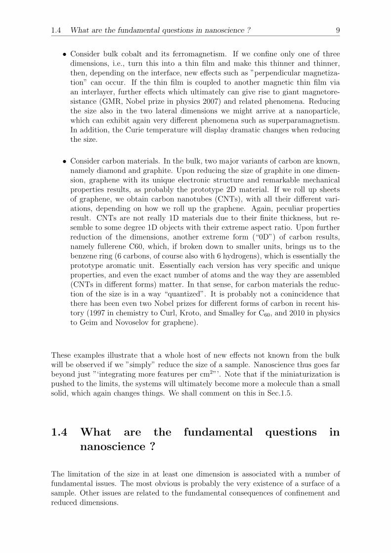
• Consider bulk CdSe and its optical absorption spectra, which for this compoundsemiconductor will be strongly determined by the electronic gap. The opticalabsorption spectra exhibit nice systematic changes when reducing the size fromthe bulk to nanoparticles of below ≈ 10 nm. The gap widens on the energyaxis, and also the oscillator strength changes. For a quantitative discussion seeJ. Jasieniak et al., J. Phys. Chem. C 113, 45 (2009).

1.4 What are the fundamental questions in nanoscience ? 9

• Consider bulk cobalt and its ferromagnetism. If we confine only one of threedimensions, i.e., turn this into a thin film and make this thinner and thinner,then, depending on the interface, new effects such as ”perpendicular magnetiza-tion” can occur. If the thin film is coupled to another magnetic thin film viaan interlayer, further effects which ultimately can give rise to giant magnetore-sistance (GMR, Nobel prize in physics 2007) and related phenomena. Reducingthe size also in the two lateral dimensions we might arrive at a nanoparticle,which can exhibit again very different phenomena such as superparamagnetism.In addition, the Curie temperature will display dramatic changes when reducingthe size.

• Consider carbon materials. In the bulk, two major variants of carbon are known,namely diamond and graphite. Upon reducing the size of graphite in one dimen-sion, graphene with its unique electronic structure and remarkable mechanicalproperties results, as probably the prototype 2D material. If we roll up sheetsof graphene, we obtain carbon nanotubes (CNTs), with all their different vari-ations, depending on how we roll up the graphene. Again, peculiar propertiesresult. CNTs are not really 1D materials due to their finite thickness, but re-semble to some degree 1D objects with their extreme aspect ratio. Upon furtherreduction of the dimensions, another extreme form (“0D”) of carbon results,namely fullerene C60, which, if broken down to smaller units, brings us to thebenzene ring (6 carbons, of course also with 6 hydrogens), which is essentially theprototype aromatic unit. Essentially each version has very specific and uniqueproperties, and even the exact number of atoms and the way they are assembled(CNTs in different forms) matter. In that sense, for carbon materials the reduc-tion of the size is in a way “quantized”. It is probably not a conincidence thatthere has been even two Nobel prizes for different forms of carbon in recent his-tory (1997 in chemistry to Curl, Kroto, and Smalley for C60, and 2010 in physicsto Geim and Novoselov for graphene).

These examples illustrate that a whole host of new effects not known from the bulkwill be observed if we ”simply” reduce the size of a sample. Nanoscience thus goes farbeyond just ”‘integrating more features per cm2”’. Note that if the miniaturization ispushed to the limits, the systems will ultimately become more a molecule than a smallsolid, which again changes things. We shall comment on this in Sec.1.5.

1.4 What are the fundamental questions in

nanoscience ?

The limitation of the size in at least one dimension is associated with a number offundamental issues. The most obvious is probably the very existence of a surface of asample. Other issues are related to the fundamental consequences of confinement andreduced dimensions.

10 Chapter 1 Introduction

1.4.1 Implications of the existence of a surface

There are several issues for which the existence of a surface, i.e. the most obviousmanifestations of the finite size of an object, introduces substantial changes or is, infact, the reason for the very occurence of an effect in the first place.

• The existence of a surface is associated with a surface energy, which, inter aliahas an impact on equilibrium shapes of nanoobjects and nanostructures.

• Enhanced reactivity at a surface, including typically unwanted reactions, such ascorrosion

• Catalysis of gas phase species induced by a surface

• ...

1.4.2 Implications of reduced size on phase transitions

The reduction of the size or the dimensions can have profound implications on phasetransitions. This is obviously a very fundamental subject with far-reaching implica-tions. Its in-depth discussion is also rather involved and connected to the work of the2016 Nobel laureates in physics, J. Michael Kosterlitz, F. Duncan M. Haldane, andDavid J. Thouless, amongst others (see also the chapter on magnetism). The reducedsize or dimensionality can change the absolute scale of the transition, i.e., the transitiontemperature TC = TC(size), as well as the nature of the transition.

This is easily illustrated using the above considerations for the density of states ofbosonic excitations, e.g., magnons for ferromagnetic materials (see chapter on mag-netism for details).

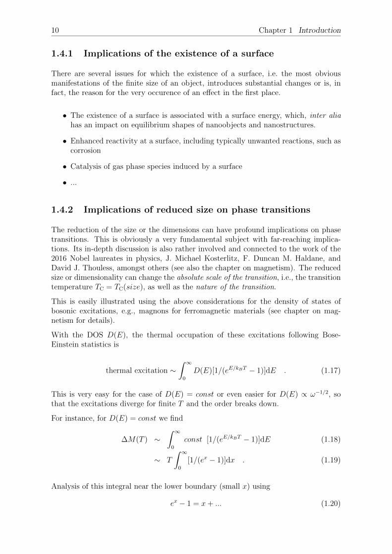
With the DOS D(E), the thermal occupation of these excitations following Bose-Einstein statistics is

thermal excitation ∼∫ ∞0

D(E)[1/(eE/kBT − 1)]dE . (1.17)

This is very easy for the case of D(E) = const or even easier for D(E) ∝ ω−1/2, sothat the excitations diverge for finite T and the order breaks down.

For instance, for D(E) = const we find

∆M(T ) ∼∫ ∞0

const [1/(eE/kBT − 1)]dE (1.18)

∼ T

∫ ∞0

[1/(ex − 1)]dx . (1.19)

Analysis of this integral near the lower boundary (small x) using

ex − 1 = x+ ... (1.20)

1.5 What are the limits of nanoscience ? 11

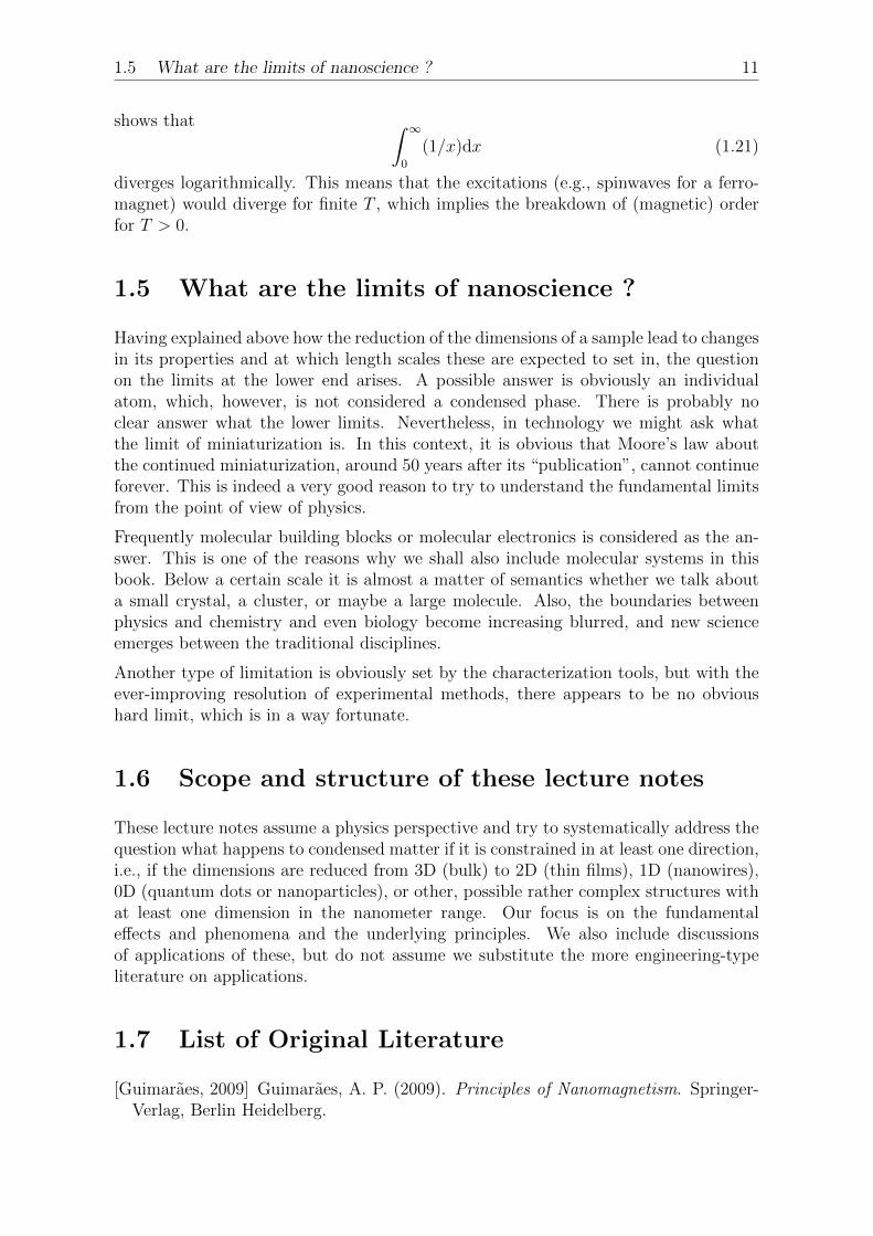
shows that ∫ ∞0

(1/x)dx (1.21)

diverges logarithmically. This means that the excitations (e.g., spinwaves for a ferro-magnet) would diverge for finite T , which implies the breakdown of (magnetic) orderfor T > 0.

1.5 What are the limits of nanoscience ?

Having explained above how the reduction of the dimensions of a sample lead to changesin its properties and at which length scales these are expected to set in, the questionon the limits at the lower end arises. A possible answer is obviously an individualatom, which, however, is not considered a condensed phase. There is probably noclear answer what the lower limits. Nevertheless, in technology we might ask whatthe limit of miniaturization is. In this context, it is obvious that Moore’s law aboutthe continued miniaturization, around 50 years after its “publication”, cannot continueforever. This is indeed a very good reason to try to understand the fundamental limitsfrom the point of view of physics.

Frequently molecular building blocks or molecular electronics is considered as the an-swer. This is one of the reasons why we shall also include molecular systems in thisbook. Below a certain scale it is almost a matter of semantics whether we talk abouta small crystal, a cluster, or maybe a large molecule. Also, the boundaries betweenphysics and chemistry and even biology become increasing blurred, and new scienceemerges between the traditional disciplines.

Another type of limitation is obviously set by the characterization tools, but with theever-improving resolution of experimental methods, there appears to be no obvioushard limit, which is in a way fortunate.

1.6 Scope and structure of these lecture notes

These lecture notes assume a physics perspective and try to systematically address thequestion what happens to condensed matter if it is constrained in at least one direction,i.e., if the dimensions are reduced from 3D (bulk) to 2D (thin films), 1D (nanowires),0D (quantum dots or nanoparticles), or other, possible rather complex structures withat least one dimension in the nanometer range. Our focus is on the fundamentaleffects and phenomena and the underlying principles. We also include discussionsof applications of these, but do not assume we substitute the more engineering-typeliterature on applications.

1.7 List of Original Literature

[Guimaraes, 2009] Guimaraes, A. P. (2009). Principles of Nanomagnetism. Springer-Verlag, Berlin Heidelberg.

12 LIST OF ORIGINAL LITERATURE

Appendix

A.1 Density of states (DOS) as a function of di-

mension d for a dipsersion ω(kn)

The important point to realise here is that the DOS D(E) depends on the dimen-sionality of the system. Let us consider the general case of excitations with energy E(frequency ω) and wave vector k, with a dispersion

E ∼ kn (A.1)

and a volume element in d-dimensional k space ∼ kd−1dk.

Using the above dispersion we write

kd−1 ∼ Ed−1/n (A.2)

Usingdk = (dk/dE)dE (A.3)

we have(dk/dE) ∼ k−nk ∼ E−1E1/n (A.4)

Thus, the volume element in k space (kd−1dk) is expressed using the volume elementin energy space

E(d−n)/ndE (A.5)

and the density of states is written as

D(E) ∼ E(d−n)/n (A.6)

13