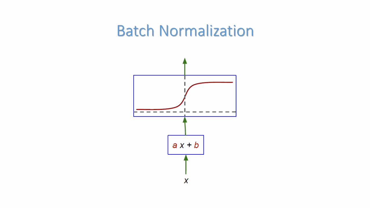
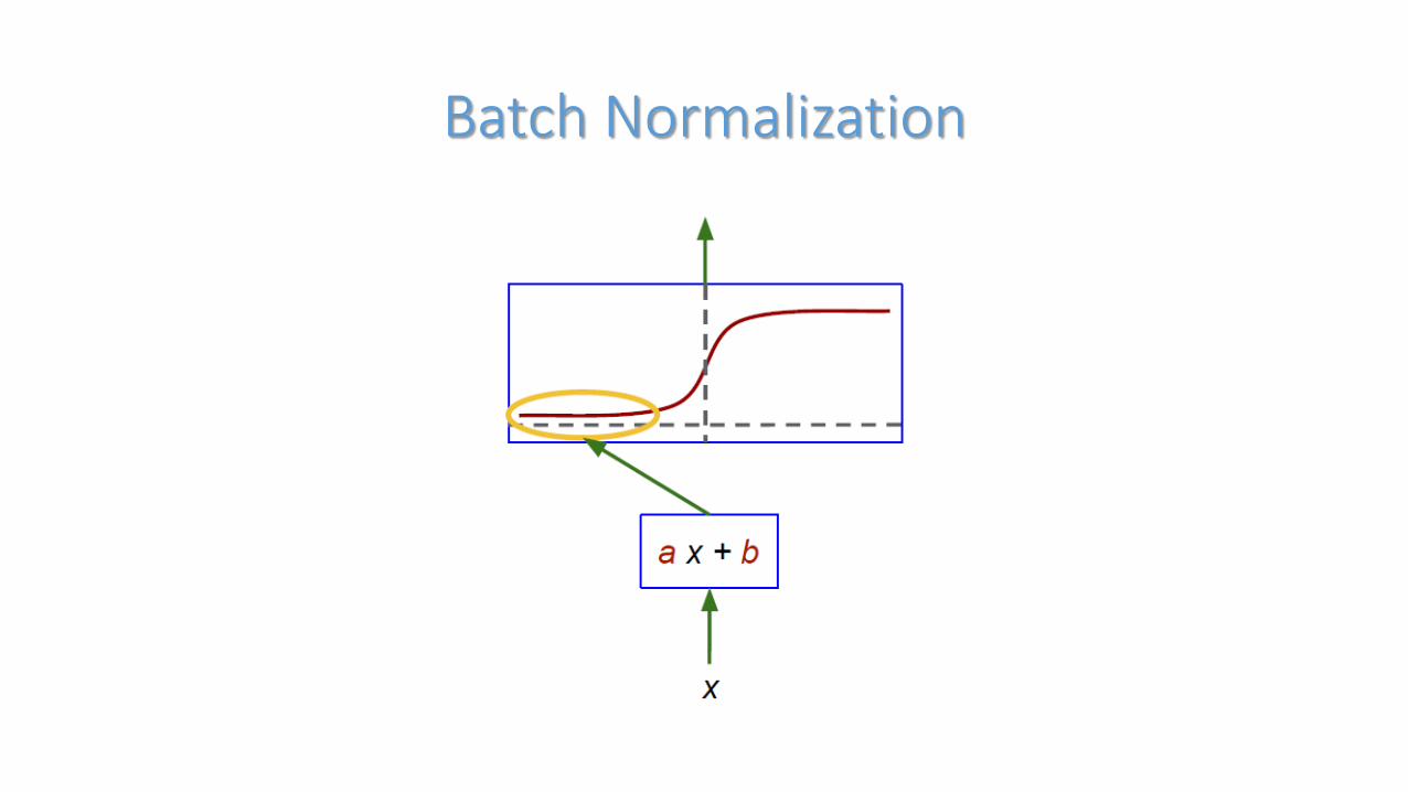
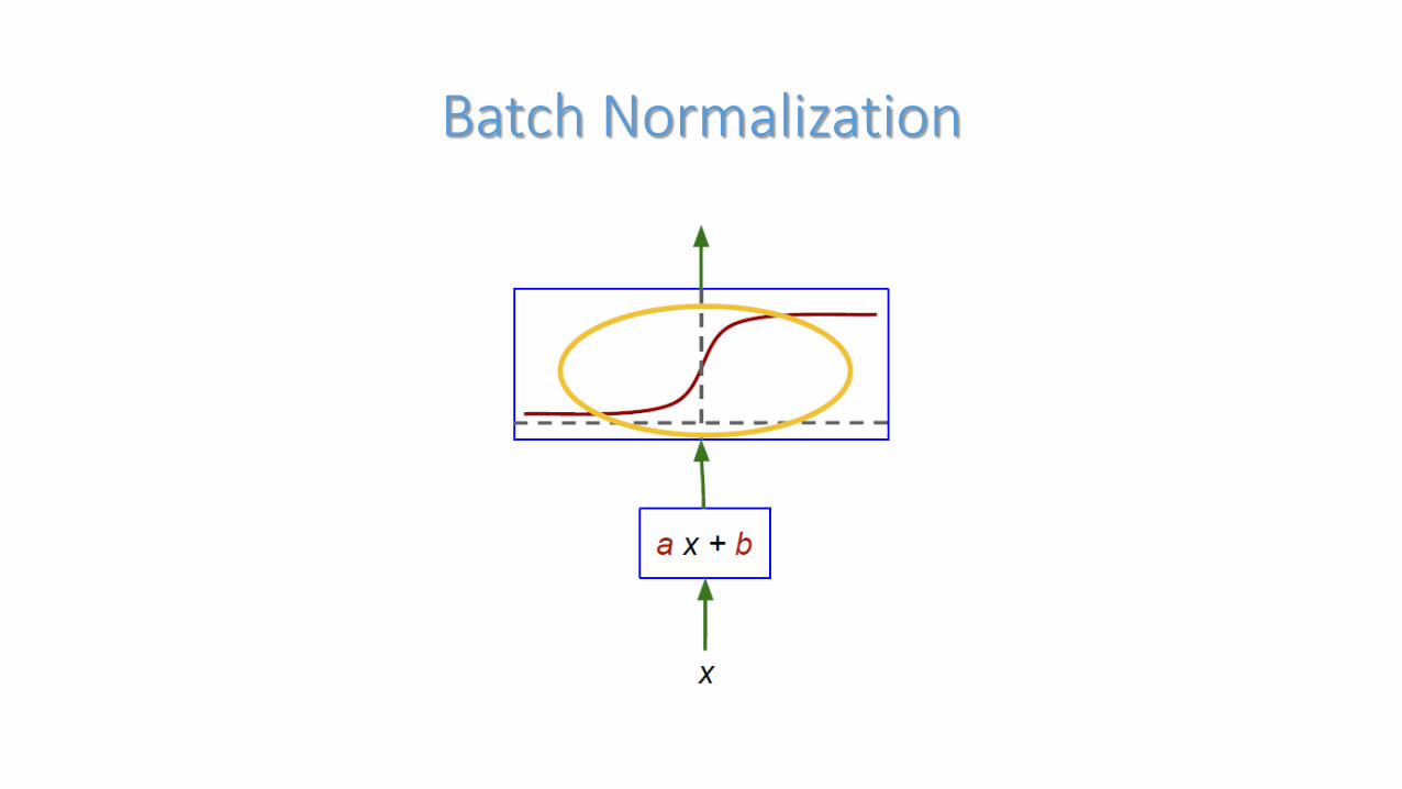
Batch Normalization

Slide modified from Sergey Ioffe , with permission

Slides based on

Batch Normalization: Accelerating Deep Network Training by Reducing Internal Covariate Shift

By Sergey Ioffe and Christian Szegedy

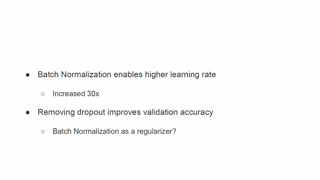
Batch Normalization

Batch Normalization

Batch Normalization

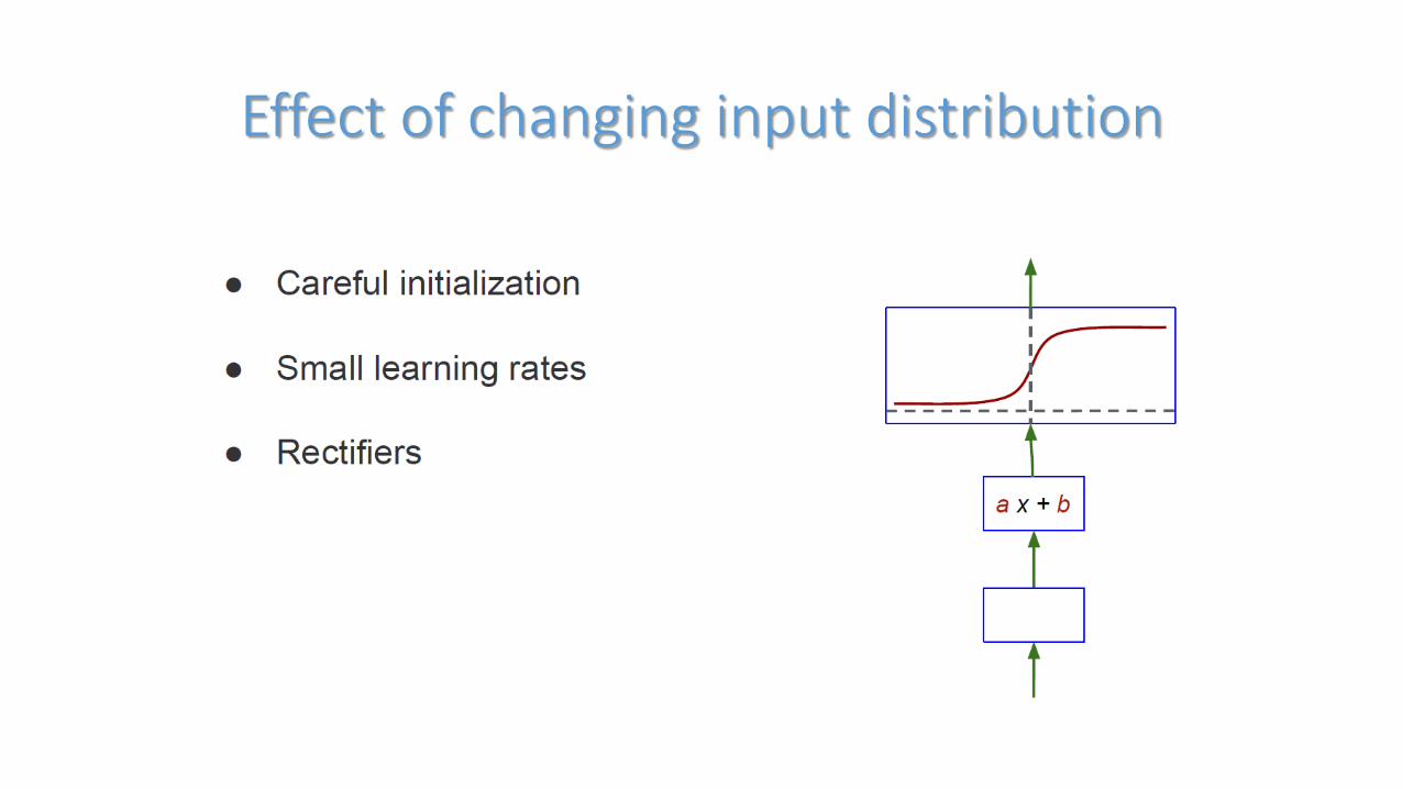
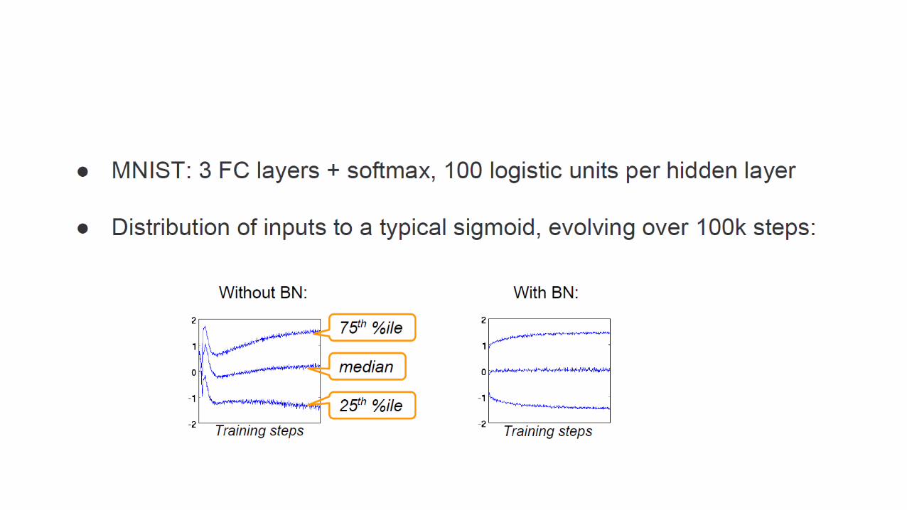
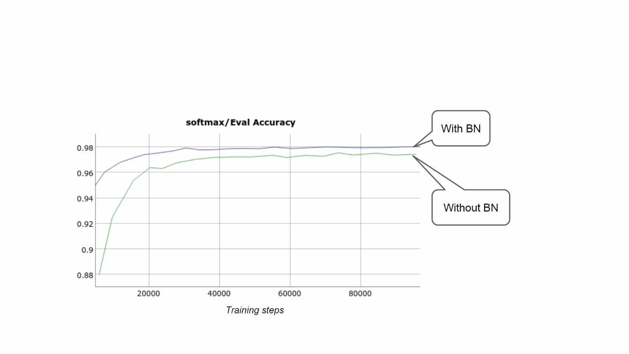
Effect of changing input distribution

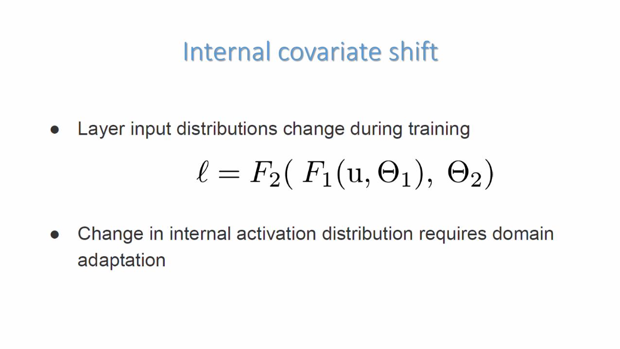
Internal covariate shift

• Some slides courtesy of Aref Jafari

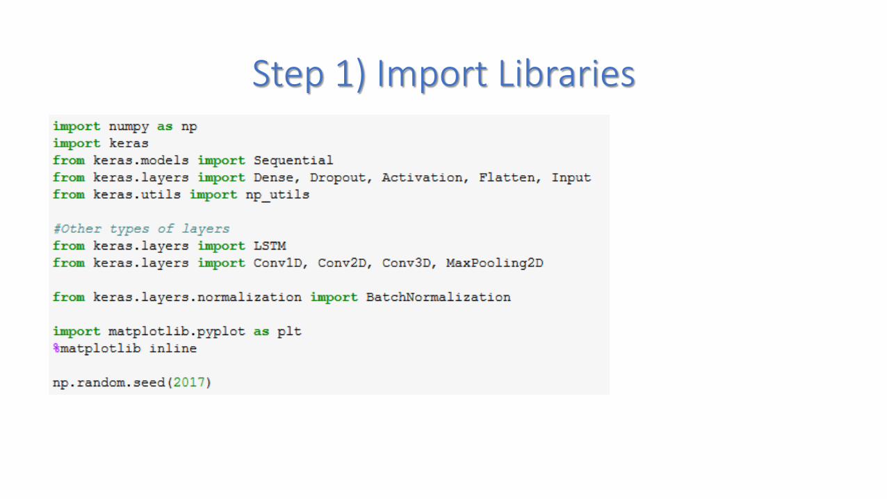
Step 1) Import Libraries

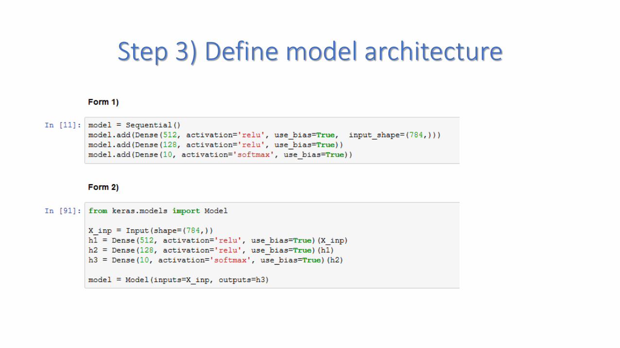
Step 3) Define model architecture

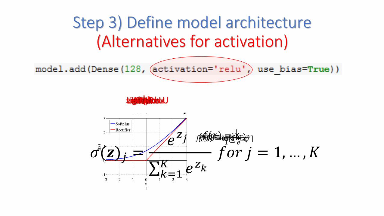
Step 3) Define model architecture(Alternatives for activation)

linear

𝑓 𝑥 = 𝑥

sigmoid

𝑓 𝑥 =1

1 − 𝑒−𝑥

tanh

𝑓 𝑥 = tanh(𝑥)

LeakyReLUrelu

𝑓 𝑥 = max(0, 𝑥)

softplus

𝑓 𝑥 = ln[1 + 𝑒𝑥]

𝜎(𝒛)𝑗 =𝑒𝑧𝑗

𝑘=1𝐾 𝑒𝑧𝑘

𝑓𝑜𝑟 𝑗 = 1,… , 𝐾

softmax

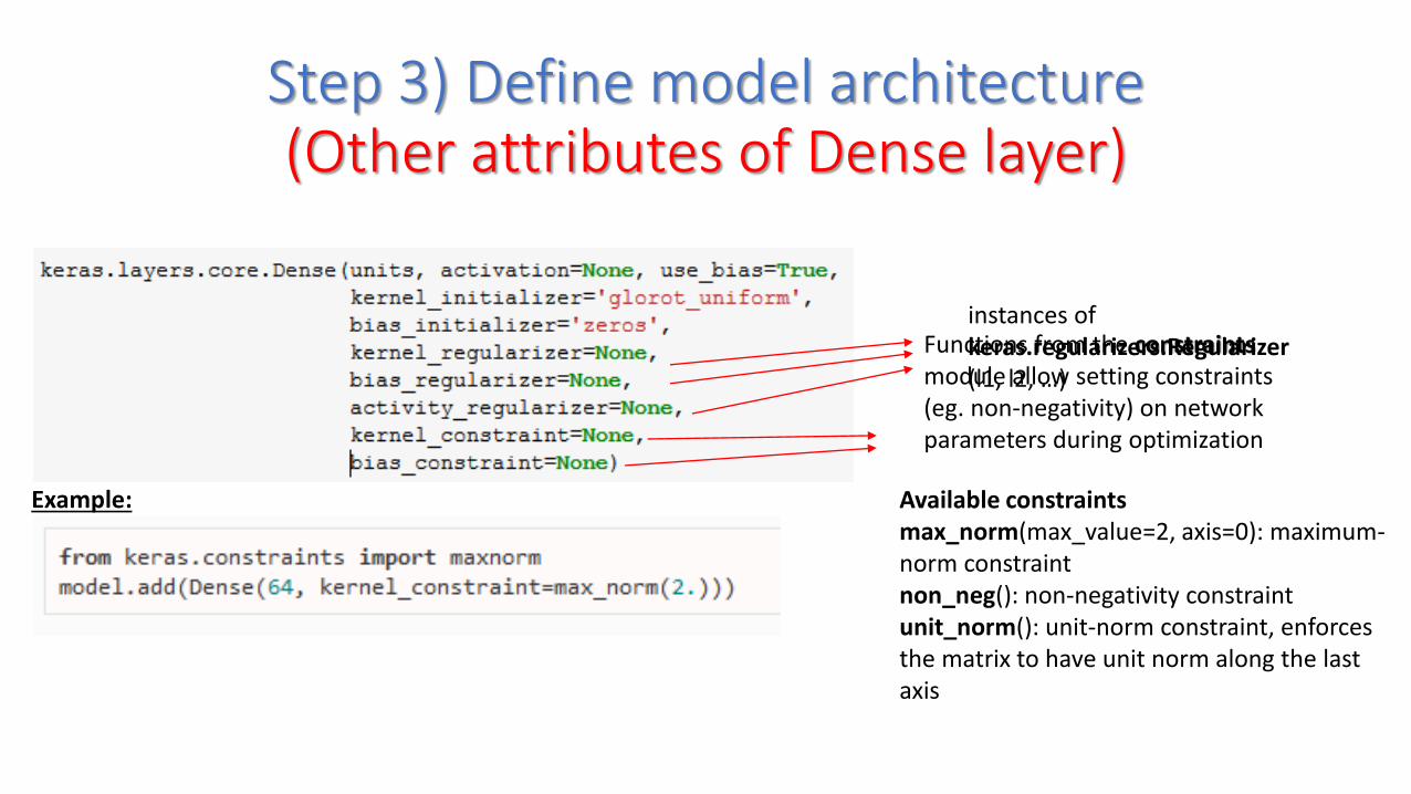
Step 3) Define model architecture(Other attributes of Dense layer)

instances of keras.regularizers.Regularizer(l1, l2, …)

Example:

Functions from the constraintsmodule allow setting constraints (eg. non-negativity) on network parameters during optimization

Available constraintsmax_norm(max_value=2, axis=0): maximum-norm constraintnon_neg(): non-negativity constraintunit_norm(): unit-norm constraint, enforces the matrix to have unit norm along the last axis

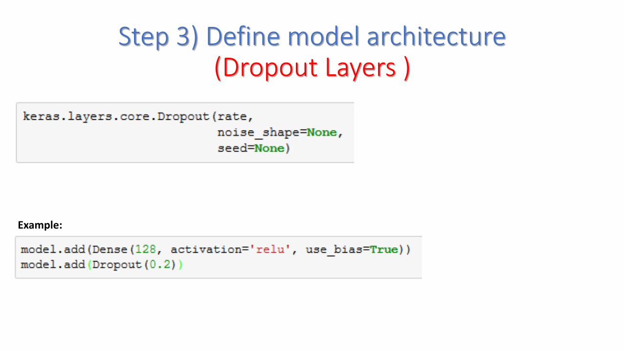
Step 3) Define model architecture(Dropout Layers )

Example:

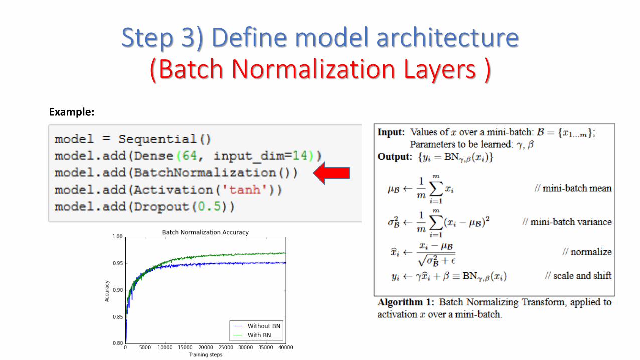
Step 3) Define model architecture(Batch Normalization Layers )

Example:

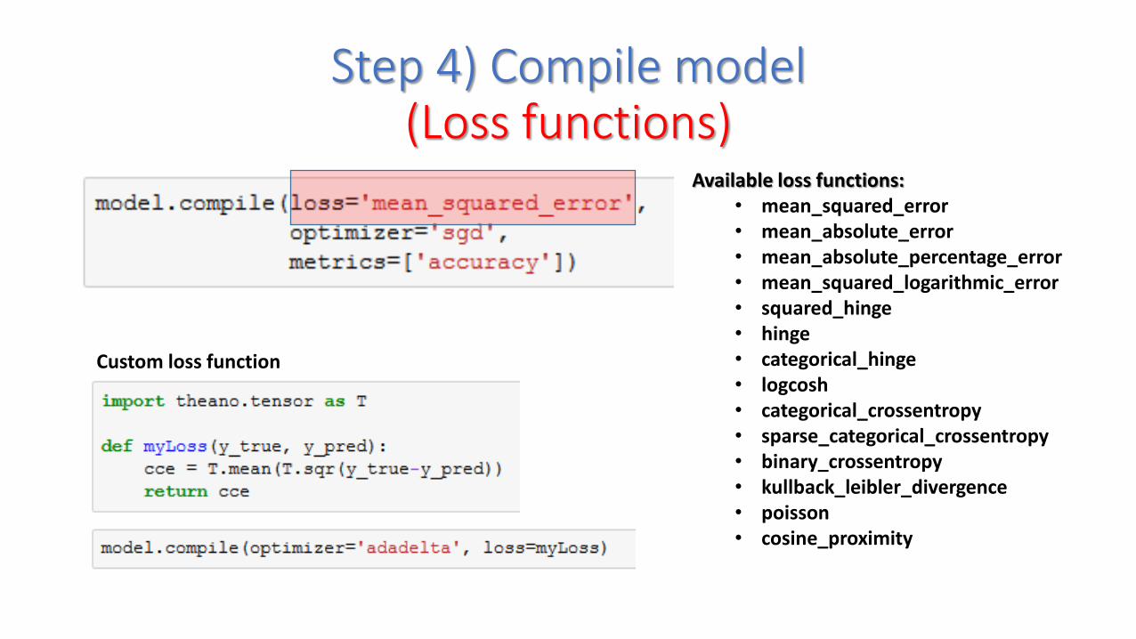
Step 4) Compile model(Loss functions)

Available loss functions:• mean_squared_error• mean_absolute_error• mean_absolute_percentage_error• mean_squared_logarithmic_error• squared_hinge• hinge• categorical_hinge• logcosh• categorical_crossentropy• sparse_categorical_crossentropy• binary_crossentropy• kullback_leibler_divergence• poisson• cosine_proximity

Custom loss function

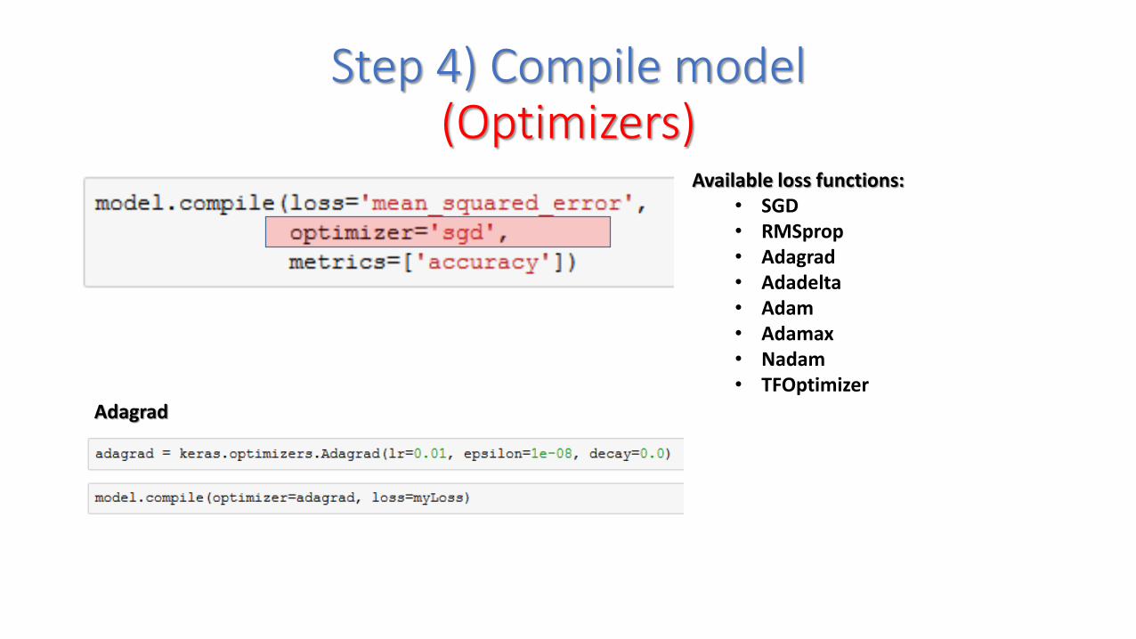
Step 4) Compile model(Optimizers)

Available loss functions:• SGD• RMSprop• Adagrad• Adadelta• Adam• Adamax• Nadam• TFOptimizer

Adagrad

Deep Learning

Convolutional Neural Network (CNNs)

Slides are partially based on Book, Deep Learning

by Bengio, Goodfellow, and Aaron Courville, 2015

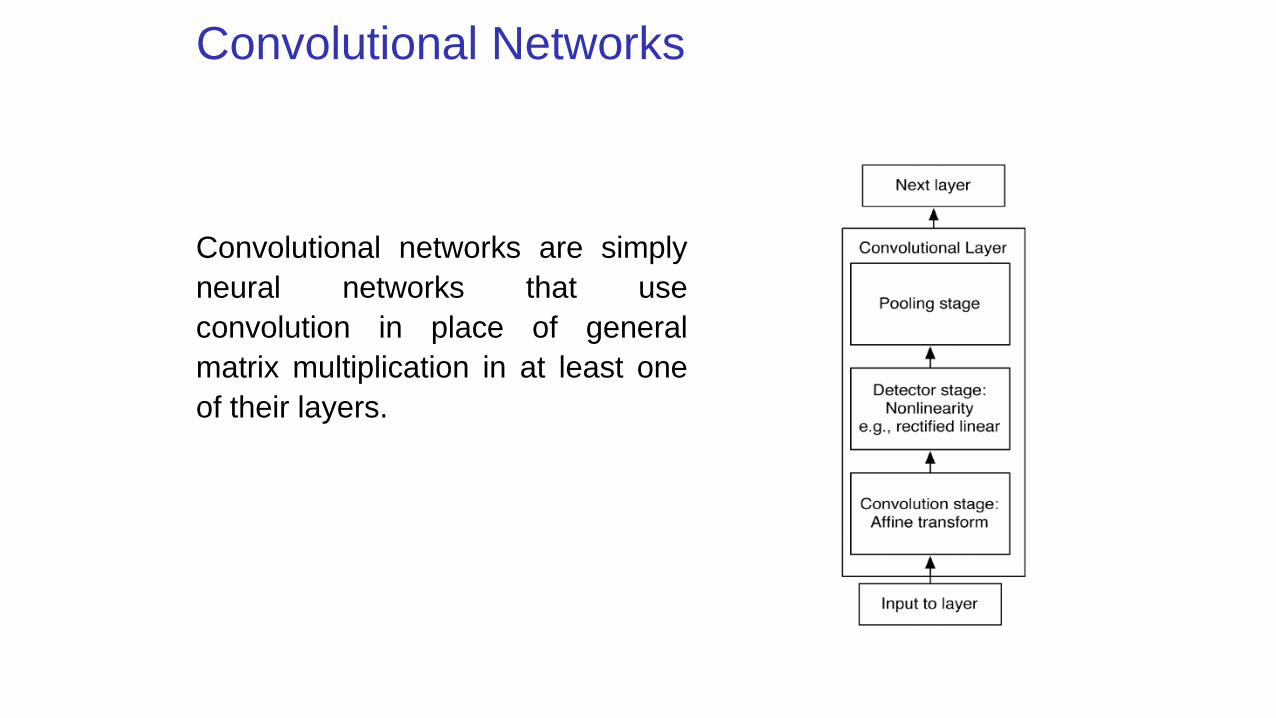
Convolutional Networks

Convolutional networks are simply

neural networks that use

convolution in place of general

matrix multiplication in at least one

of their layers.

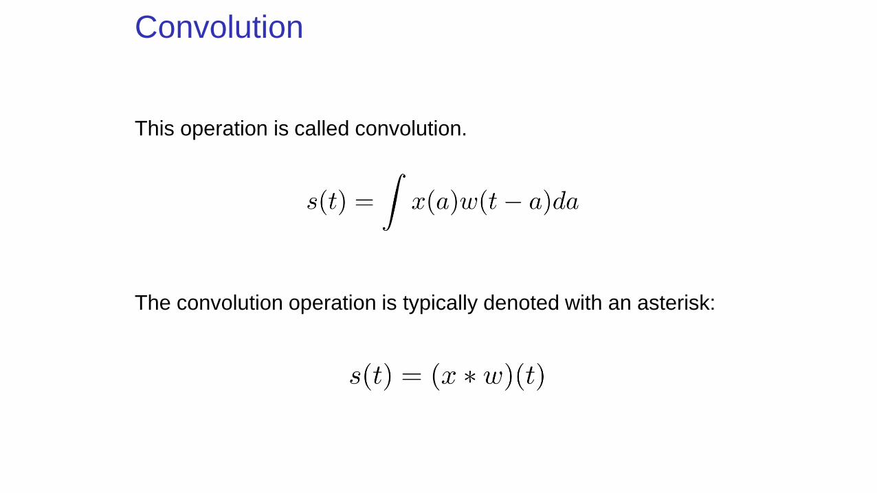
Convolution

This operation is called convolution.

The convolution operation is typically denoted with an asterisk:

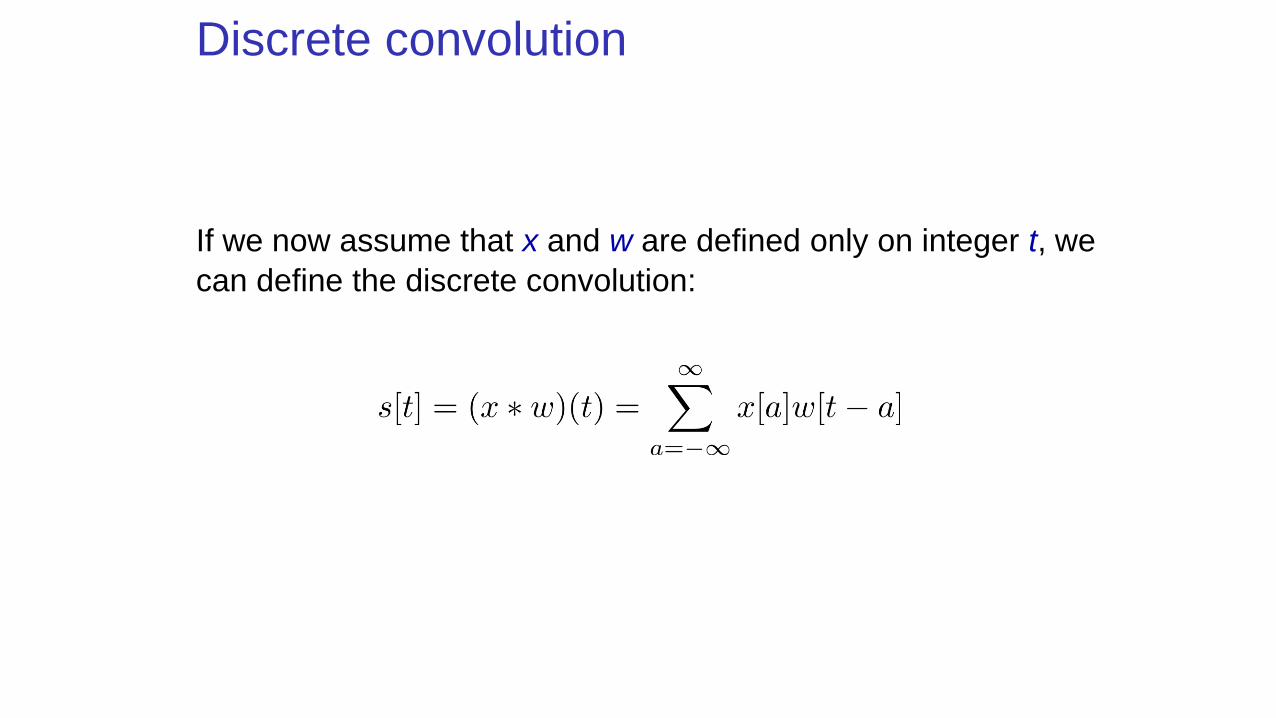
Discrete convolution

If we now assume that x and w are defined only on integer t, we

can define the discrete convolution:

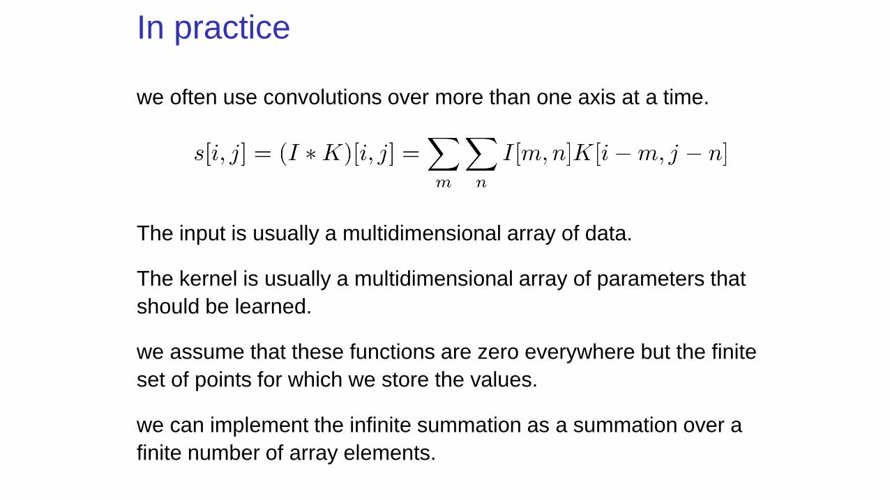
In practice

we often use convolutions over more than one axis at a time.

The input is usually a multidimensional array of data.

The kernel is usually a multidimensional array of parameters that

should be learned.

we assume that these functions are zero everywhere but the finite

set of points for which we store the values.

we can implement the infinite summation as a summation over a

finite number of array elements.

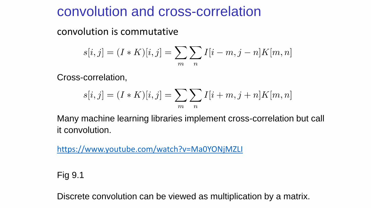
convolution and cross-correlation

convolution is commutative

Cross-correlation,

Many machine learning libraries implement cross-correlation but call

it convolution.

https://www.youtube.com/watch?v=Ma0YONjMZLI

Fig 9.1

Discrete convolution can be viewed as multiplication by a matrix.

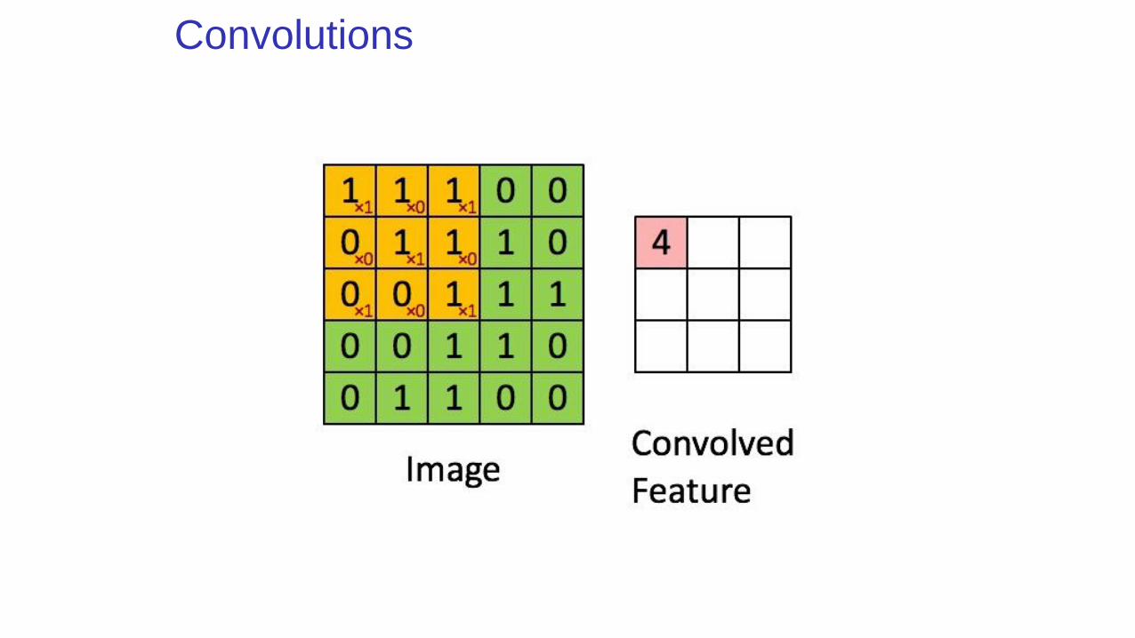
Convolutions

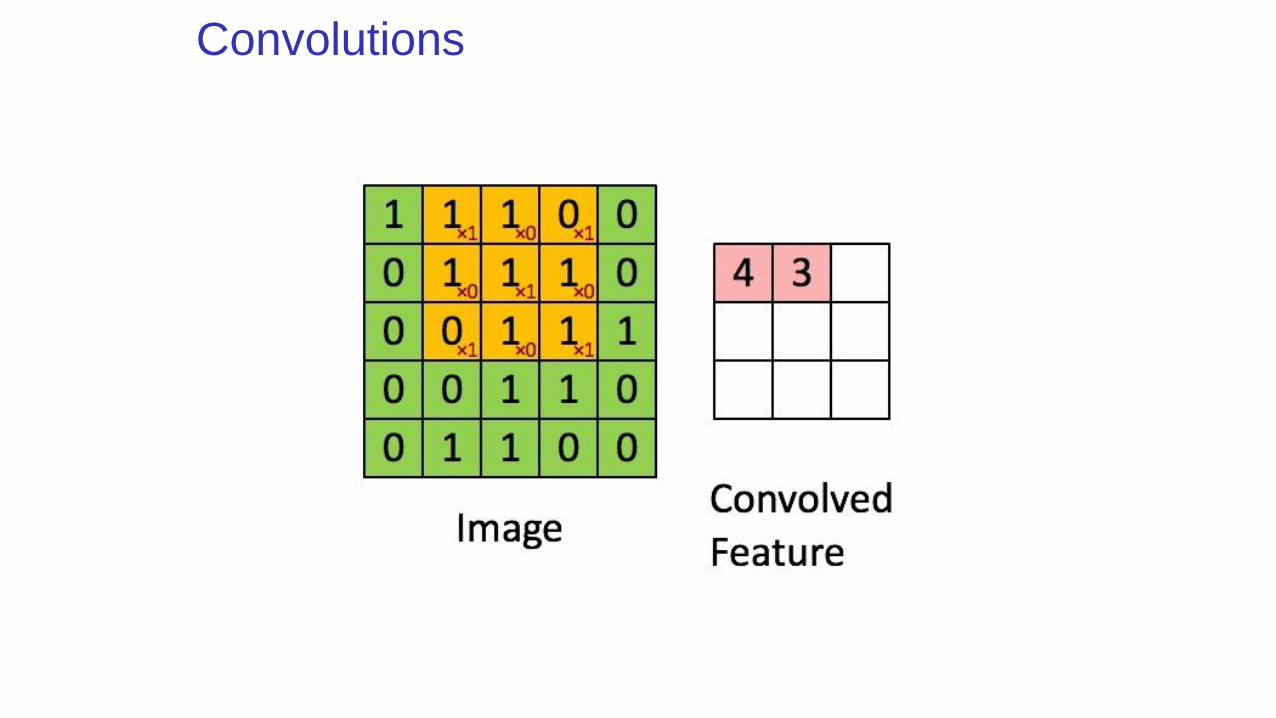
Convolutions

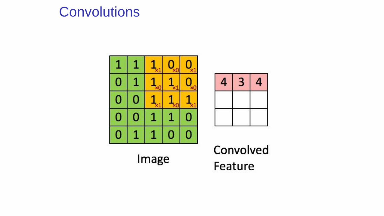
Convolutions

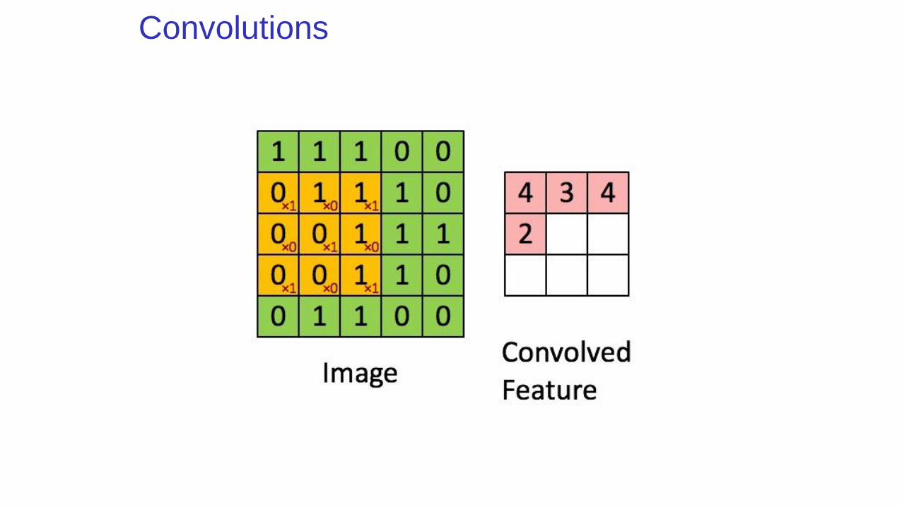
Convolutions

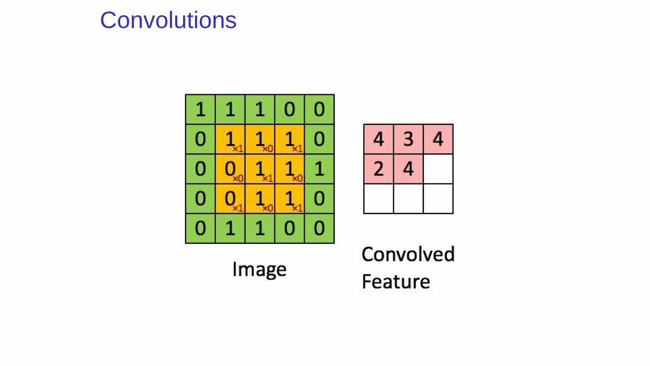
Convolutions

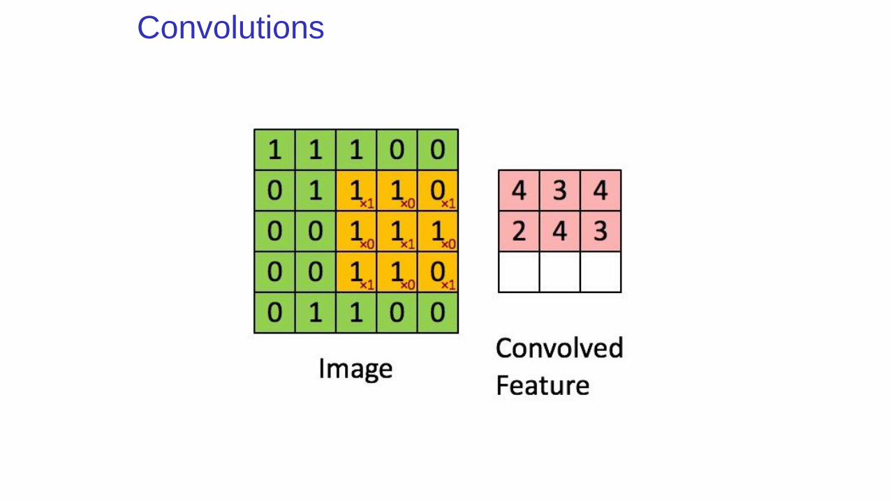
Convolutions

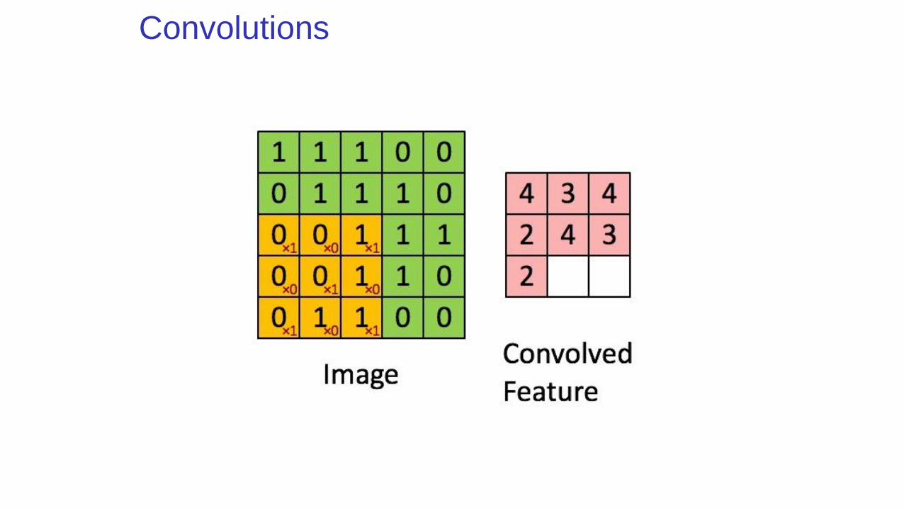
Convolutions

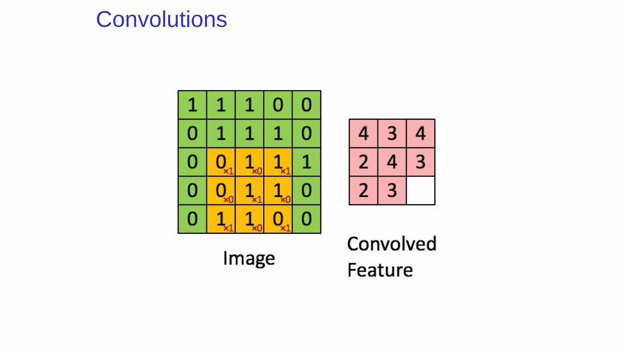
Convolutions

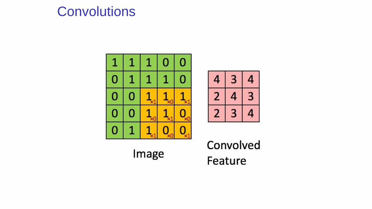
Convolutions

Sparse interactions

In feed forward neural network every output unit interacts with every input unit.

Convolutional networks, typically have sparse connectivity ( sparse weights)

This is accomplished by making the kernel smaller than the input

Sparse interactions

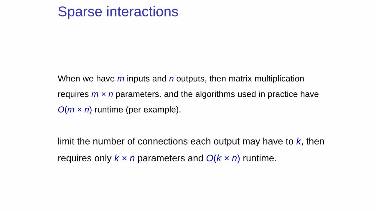
When we have m inputs and n outputs, then matrix multiplication

requires m × n parameters. and the algorithms used in practice have

O(m × n) runtime (per example).

limit the number of connections each output may have to k, then

requires only k × n parameters and O(k × n) runtime.

Parameter sharing

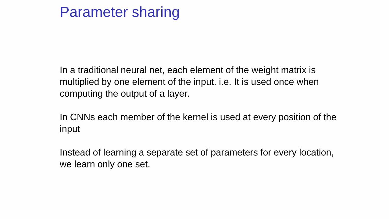
In a traditional neural net, each element of the weight matrix is

multiplied by one element of the input. i.e. It is used once when

computing the output of a layer.

In CNNs each member of the kernel is used at every position of the

input

Instead of learning a separate set of parameters for every location,

we learn only one set.

Equivariance

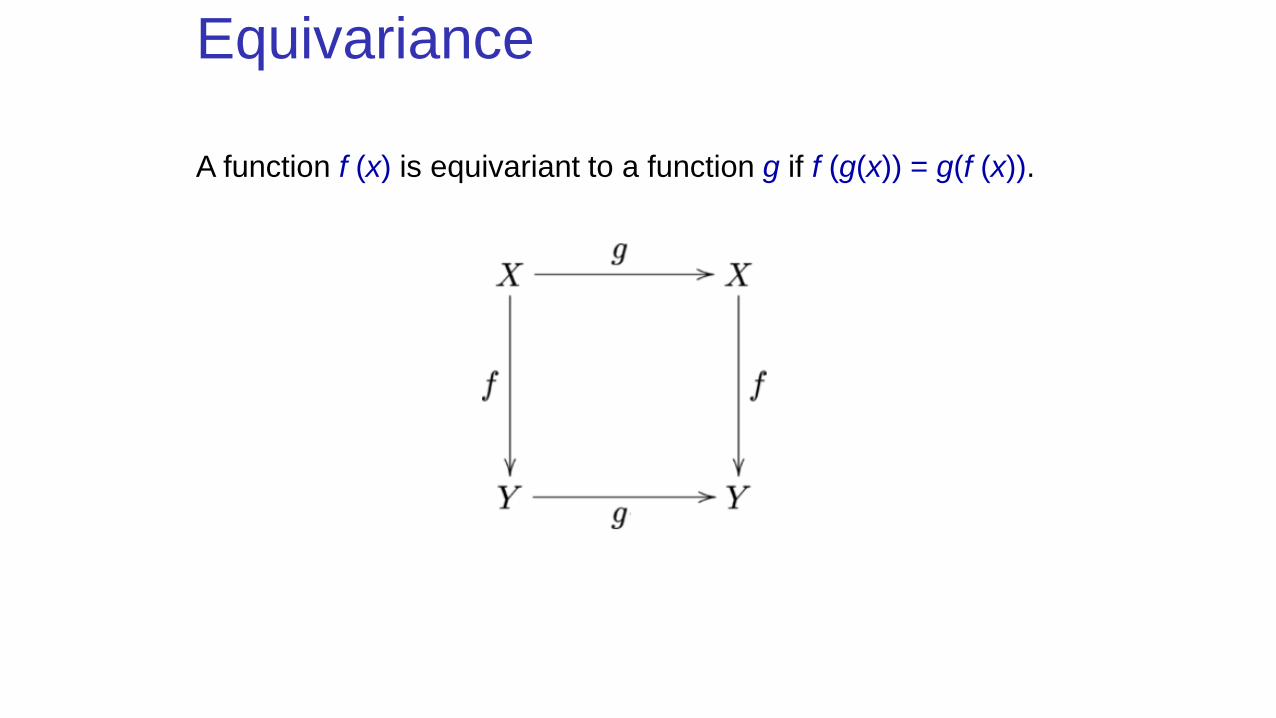
A function f (x) is equivariant to a function g if f (g(x)) = g(f (x)).

Equivariance

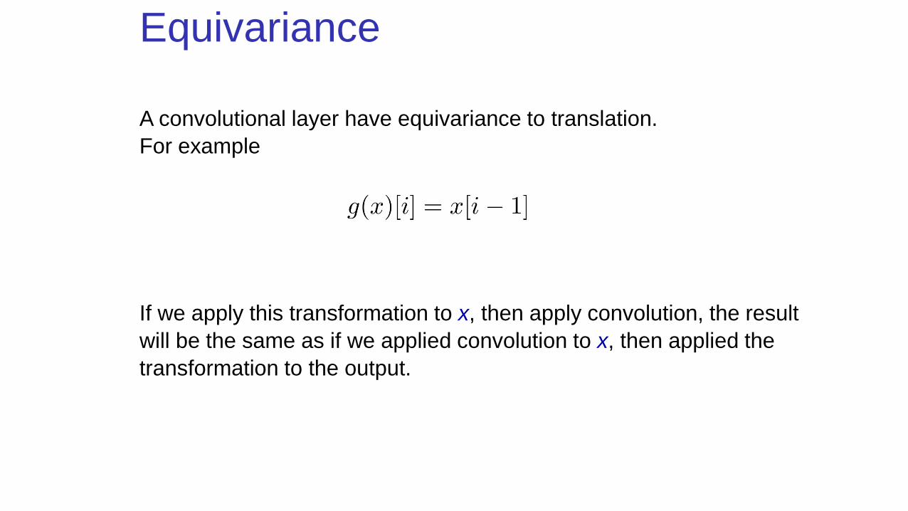
A convolutional layer have equivariance to translation.

For example

If we apply this transformation to x, then apply convolution, the result

will be the same as if we applied convolution to x, then applied the

transformation to the output.

Equivariance

For images, convolution creates a 2-D map of where certain features

appear in the input.

Note that convolution is not equivariant to some other

transformations, such as changes in the scale or rotation of an

image.

Convolutional Networks

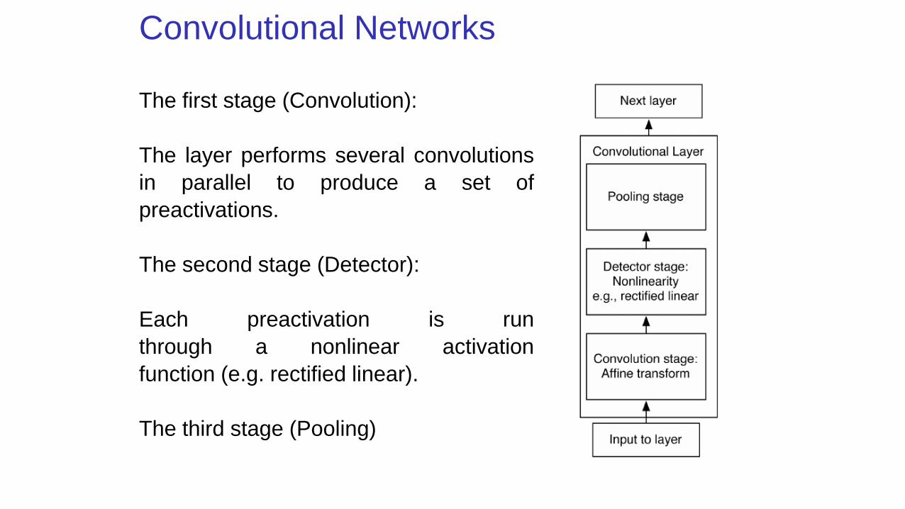
The first stage (Convolution):

The layer performs several convolutions

in parallel to produce a set of

preactivations.

The second stage (Detector):

Each preactivation is run

through a nonlinear activation

function (e.g. rectified linear).

The third stage (Pooling)

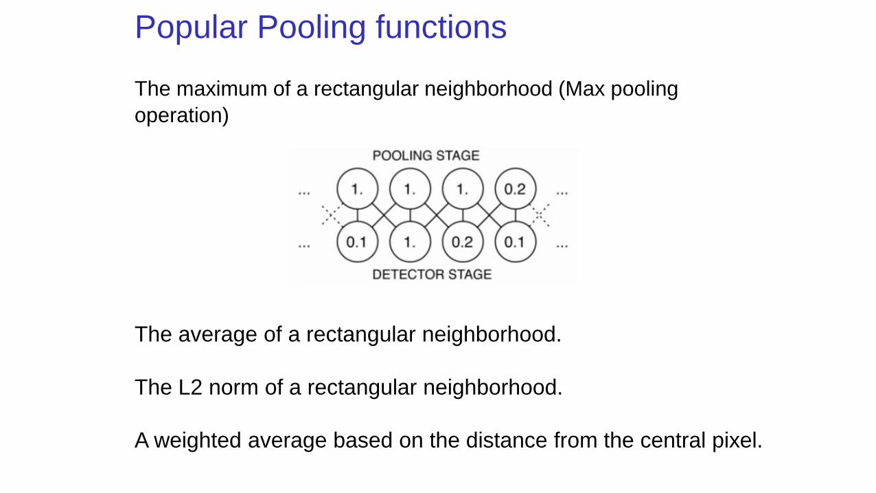
Popular Pooling functions

The maximum of a rectangular neighborhood (Max pooling

operation)

The average of a rectangular neighborhood.

The L2 norm of a rectangular neighborhood.

A weighted average based on the distance from the central pixel.

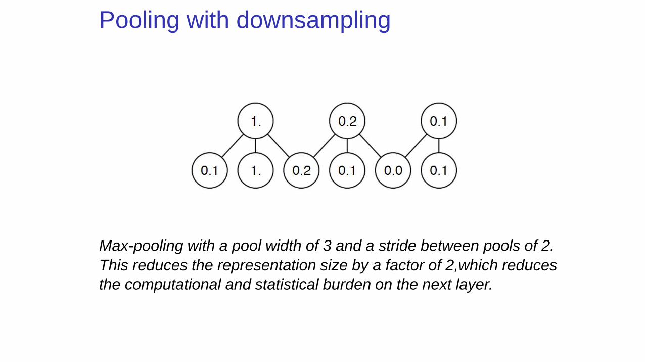
Pooling with downsampling

Max-pooling with a pool width of 3 and a stride between pools of 2.

This reduces the representation size by a factor of 2,which reduces

the computational and statistical burden on the next layer.