Batch Splitting in an Assembly Scheduling Environment

Satyaki Ghosh Dastidar • Rakesh Nagi1

420 Bell Hall, Department of Industrial Engineering, University at Buffalo (SUNY),Buffalo, NY 14260, USA.

This paper presents mathematical models and algorithms for a production scheduling prob-lem with batch splitting of assembly operations. The operation precedence is representedin an operations network, and the operations at any particular workcenter are split intosuitable batch sizes on the available identical parallel processors for faster completion. Thesolution methodology comprises of a batch splitting algorithm followed by a batch schedul-ing algorithm. The batch splitting algorithm is developed based on a preemptive schedulingalgorithm after incorporating non-zero setup times. The batch scheduling algorithm is basedon a Critical Path algorithm for an operations network. The mathematical model also con-siders movesizes for batches which determine the threshold for the batch size that needsto be built up before it can be transferred for the successor operation. The computationalresults for different problem sizes show that the proposed solution scheme can satisfactorilysolve this complex scheduling problem for cases where the standard solvers fail to generatesolutions within practical time limits. Moreover, there is a significant reduction in makespandue to batch splitting.

Keywords: Batch Splitting, Assembly Scheduling, Movesize.

1. Introduction

The primary focus of most manufacturing enterprises in recent times has been on customer

needs. This has resulted in a shift from the conventional strategy of mass production to

batch production. Due to continuously varying customer demands, products are being man-

ufactured in small batches and the diversity of the product mix has made the production

planning and scheduling more complex. In the current competitive environment, more and

more emphasis is being placed on the reduction of lead time, production and setup costs,

and timely delivery. Although there have been advances in production control techniques,

for a multi-stage manufacturing environment, Materials Requirements Planning (MRP) con-

tinues to remain popular in industry. However, MRP generally does not consider capacity

constraints and assumes fixed production lead times that are not realistic. One can minimize

1Author for correspondence. E-mail: nagi@buffalo.edu; Tel: 1-716-645-2357 x 2103; Fax: 1-716-645-3302.

1

the makespan by creating sub-lots and by overlapping the operations using frequent mate-

rial movement. This process is known as lot-splitting or lot-streaming and is also helpful in

reducing the total lead time and the total Work-In-Process (WIP).

2. Literature Review

A classical approach in production planning and scheduling is to derive a Master Production

Schedule (MPS). The release dates are then calculated and a schedule is planned from the

bill-of-material (BOM) of the MRP module. Dauzere-Peres and Lasserre (1994) show that

in a job shop environment, the knowledge of detailed constraints in the MPS module is very

limited and hence it might lead to unachievable production plans. In a multi-stage production

environment, the lead times are retrieved or computed for all the items which are then used

by MRP to determine the start dates for manufacturing shop orders. These schedules are

frequently infeasible due to the assumed lead times. Traditional MRP, as described by

Orlicky (1975), assumes that once a batch is started on a workcenter, the entire batch is

completed before any part of it is sent to the next workcenter. With the creation of sub-lots

we can overlap operations. The sub-lots are transported for the next operation (usually to

the next workcenter) while the remainder of the batch is being processed. This process of

creating sub-lots and overlapping the operations is called lot streaming. This is helpful in

reducing the total lead time and the total WIP. Lot splitting is a complex problem where a

setup is required every time a lot is split among the functionally identical processors. Lot

splitting can also help reduce the total lead time due to parallelism. However, in presence

of non-zero setup times, the lot splitting strategy can increase the makespan due to the

additional setup time for every such lots being created. Judicious lot-splitting is essential

due to the increase in work content, but potential of significant reduction in lead times and

inventory.

Ongoing research in the area of lot-splitting indicates that the popularity of lot-splitting

has grown following the success of cellular manufacturing. Several types of lot-splitting

schemes have been described in the literature. Graves and Kostreva (1986) gave the notion

of “overlapping operations” in MRP. They derive the optimal sizes for lot transfers of the

overlapping operations by considering a generic two-workstation segment of a manufacturing

system. They solve for the optimal production batch size, the optimal transfer batch size, and

the integral multiple relating these. Jacobs and Bragg (1988) proposed that transfer batch

2

sizes be integral multiples of the production batch sizes. Baker and Pyke (1990) considered

two cases of lot splitting: (i) Preemption (interrupt production run for a more urgent job);

and (ii) Lot Streaming (overlapping operations). They presented a solution algorithm for the

lot streaming problem with two sub lots. Kropp and Smunt (1990) presented some optimal

and heuristic models for lot-splitting in a flow shop environment (single job) using a quadratic

programming approach. Wagner and Ragatz (1994) determined the impact of lot splitting

on due date performance (open job shop environment). They used simulation experiments to

draw their conclusions. They showed that the lot-splitting impact improved monotonically

with decreasing transfer batch size. Agrawal et al. (2000) incorporates movesizes in their

formulation. Movesizes determine the threshold for the batch size that needs to be built up

before it can be transferred for the successor operation.

The current use of MRP systems in a multi-stage, multi-product production environment

is not focused on the need for lot sizing at each level of the component BOM. MRP ignores

the detailed shop floor capacity and usually assumes fixed lead time which might not be

feasible. The lot-sizing formulations can be extended for batch splitting due to similarity

in objectives (set up and inventory costs). In addition, batch splitting helps reduce the

makespan. Baker and Trietsch (1993) demonstrate some basic techniques for lot streaming

in different production scheduling environments. Botsali (1999) has classified the various

lot streaming techniques used in production scheduling. Yavuz (1999) presents a fairly

exhaustive review of the performance various scheduling models and algorithms with batch

splitting and lot-sizing for the production scheduling problems.

The various batch splitting (lot streaming) models and algorithms in the literature con-

sider the effect of sublots on the makespan. The effect of transfer sizes (movesizes), batch

splitting (lot streaming) and batch overlapping has been studied to some extent. Several

algorithms have been proposed to decide on the batch splitting strategies. Most of these

models emphasize on batch-splitting strategies based on various heuristic approaches with-

out proper focus on the analytical modeling. There seems to be no proper mathematical

model that incorporates batch splitting and movesizes along with non-zero setup times, in

an integrated manner. Consequently, there seems to be a lack of easy-to-implement algo-

rithms that address and solve the integrated batch-splitting and batch-scheduling problem

along with realistic scheduling constraints like transfer sizes and non-zero setup times. This

constitutes the focus and contribution of this paper.

3

3. Problem Description and Formulation

This section presents the preliminaries of representing assembly operations and two mathe-

matical programming models that represent batch splitting without consideration of move ize

and with its consideration. Lastly, with the help of an illustrative example, we demonstrate

the application of these formulations and the benefit of their respective strategies.

3.1 Network Representation of Precedence Relationships

A precedence network represents the precedence relationships among operations, for each

end item, can be obtained from the BOM and part routings (Agrawal et al., 1996). Each

manufactured part is assumed to have a unique sequence of operations (routing) required to

process it.

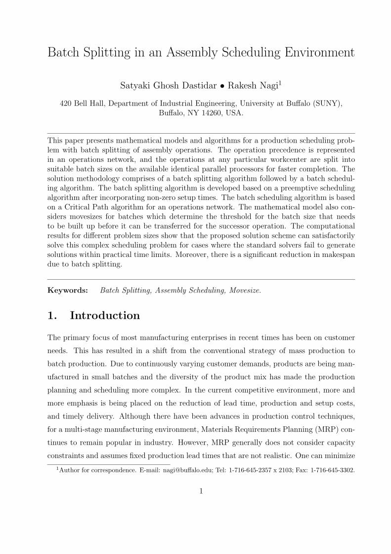
Figure 1 shows a typical BOM structure for a part A. The routing information for manu-

factured or assembled parts is shown in Table 1. For simplicity, we assume that manufactured

parts A, B, C and D each have one operation in their routings, while E, F and G each have

two operations in their routings.

Part: C

Type: MakeQty: 10Part: D

Part: AQty: 1

Type: Assembly

Qty: 1 Qty: 1 Qty: 1Part: H

Type: Purchase Type: Purchase Type: Purchase

Part: I Part: J

Part: E Part: F Part: GQty: 1 Qty: 1 Qty: 1

Type: Make Type: Make Type: Make

Qty: 10Part: B

Type: MakeQty: 10

Type: Make

Figure 1: Bill-of-Materials (BOM) of the final product A.

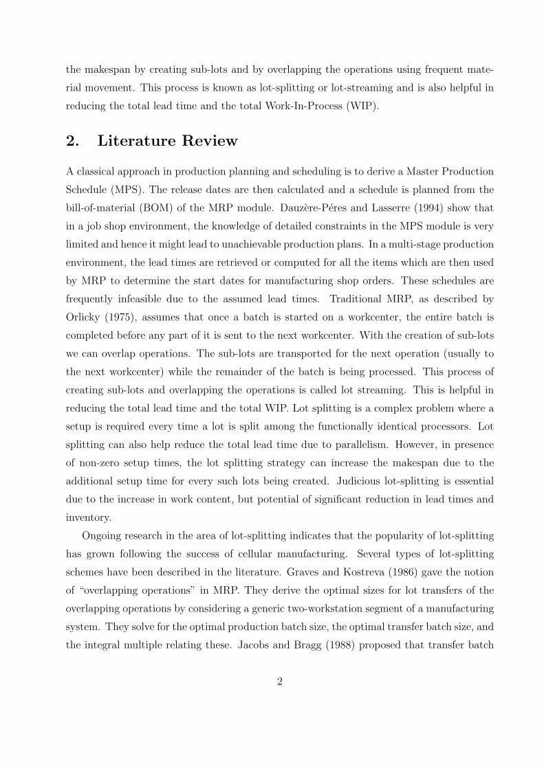
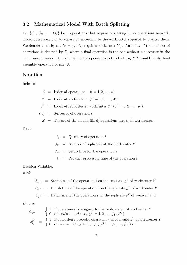
Figure 2 combines the BOM and the routing information to obtain the precedence net-

work of operations corresponding to part A. This operations network forms the basis of the

two mathematical programming models presented in the following. They attempt to mini-

mize the production makespan with judicious batch splitting of operations (without or with

consideration of move size). The assumption we follow is that a batch of operations would

at most be split among the multiple machines/replicates of the required workcenter. We do

4

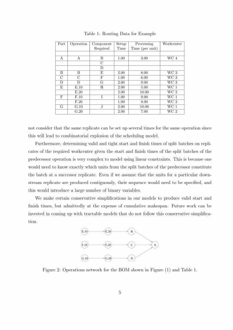
Table 1: Routing Data for Example

Part Operation Component Setup Processing WorkcenterRequired Time Time (per unit)

A A B 1.00 3.00 WC 4CD

B B E 2.00 8.00 WC 3C C F 1.00 6.00 WC 3D D G 2.00 9.00 WC 3E E.10 H 2.00 5.00 WC 1

E.20 2.00 10.00 WC 2F F.10 I 1.00 9.00 WC 1

F.20 1.00 8.00 WC 2G G.10 J 2.00 10.00 WC 1

G.20 2.00 7.00 WC 2

not consider that the same replicate can be set up several times for the same operation since

this will lead to combinatorial explosion of the scheduling model.

Furthermore, determining valid and tight start and finish times of split batches on repli-

cates of the required workcenter given the start and finish times of the split batches of the

predecessor operation is very complex to model using linear constraints. This is because one

would need to know exactly which units from the split batches of the predecessor constitute

the batch at a successor replicate. Even if we assume that the units for a particular down-

stream replicate are produced contiguously, their sequence would need to be specified, and

this would introduce a large number of binary variables.

We make certain conservative simplifications in our models to produce valid start and

finish times, but admittedly at the expense of cumulative makespan. Future work can be

invested in coming up with tractable models that do not follow this conservative simplifica-

tion.

D

A

B

G.20

F.20

E.20

CF.10

E.10

G.10

Figure 2: Operations network for the BOM shown in Figure (1) and Table 1.

5

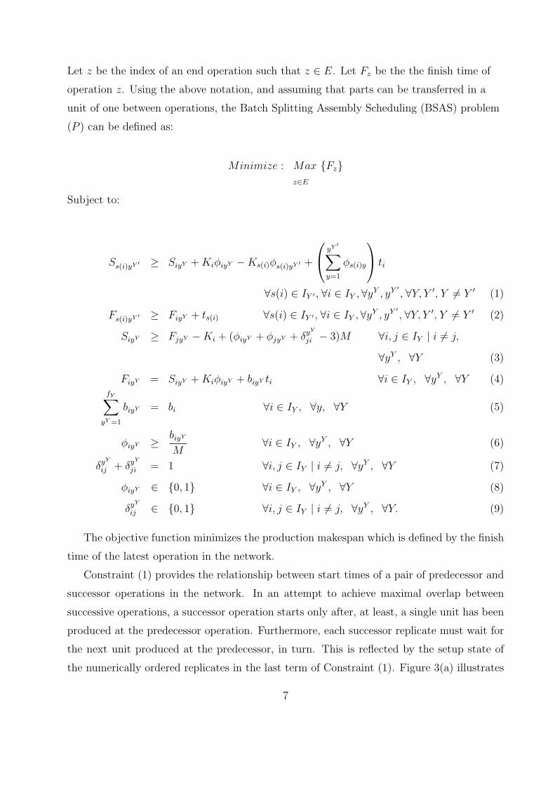
3.2 Mathematical Model With Batch Splitting

Let {O1, O2, . . . , On} be n operations that require processing in an operations network.

These operations can be separated according to the workcenter required to process them.

We denote these by set IY = {j: Oj requires workcenter Y }. An index of the final set of

operations is denoted by E, where a final operation is the one without a successor in the

operations network. For example, in the operations network of Fig. 2 E would be the final

assembly operation of part A.

Notation

Indexes:

i = Index of operations (i = 1, 2, . . . , n)

Y = Index of workcenters (Y = 1, 2, . . . ,W )

yY = Index of replicates at workcenter Y (yY = 1, 2, . . . , fY )

s(i) = Successor of operation i

E = The set of the all end (final) operations across all workcenters

Data:

bi = Quantity of operation i

fY = Number of replicates at the workcenter Y

Ki = Setup time for the operation i

ti = Per unit processing time of the operation i

Decision Variables:

Real:

SiyY = Start time of the operation i on the replicate yY of workcenter Y

FiyY = Finish time of the operation i on the replicate yY of workcenter Y

biyY = Batch size for the operation i on the replicate yY of workcenter Y

Binary:

φiyY =

{

1 if operation i is assigned to the replicate yY of workcenter Y

0 otherwise (∀i ∈ IY , yY = 1, 2, . . . , fY ,∀Y )

δyY

ij =

{

1 if operation i precedes operation j at replicate yY of workcenter Y

0 otherwise (∀i, j ∈ IY , i 6= j, yY = 1, 2, . . . , fY ,∀Y )

6

Let z be the index of an end operation such that z ∈ E. Let Fz be the the finish time of

operation z. Using the above notation, and assuming that parts can be transferred in a

unit of one between operations, the Batch Splitting Assembly Scheduling (BSAS) problem

(P ) can be defined as:

Minimize : Max {Fz}

z∈E

Subject to:

Ss(i)yY ′ ≥ SiyY + KiφiyY − Ks(i)φs(i)yY ′ +

yY′

∑

y=1

φs(i)y

ti

∀s(i) ∈ IY ′ , ∀i ∈ IY ,∀yY , yY ′

, ∀Y, Y ′, Y 6= Y ′ (1)

Fs(i)yY ′ ≥ FiyY + ts(i) ∀s(i) ∈ IY ′ , ∀i ∈ IY ,∀yY , yY ′

, ∀Y, Y ′, Y 6= Y ′ (2)

SiyY ≥ FjyY − Ki + (φiyY + φjyY + δyY

ji − 3)M ∀i, j ∈ IY | i 6= j,

∀yY , ∀Y (3)

FiyY = SiyY + KiφiyY + biyY ti ∀i ∈ IY , ∀yY , ∀Y (4)fY∑

yY =1

biyY = bi ∀i ∈ IY , ∀y, ∀Y (5)

φiyY ≥biyY

M∀i ∈ IY , ∀yY , ∀Y (6)

δyY

ij + δyY

ji = 1 ∀i, j ∈ IY | i 6= j, ∀yY , ∀Y (7)

φiyY ∈ {0, 1} ∀i ∈ IY , ∀yY , ∀Y (8)

δyY

ij ∈ {0, 1} ∀i, j ∈ IY | i 6= j, ∀yY , ∀Y. (9)

The objective function minimizes the production makespan which is defined by the finish

time of the latest operation in the network.

Constraint (1) provides the relationship between start times of a pair of predecessor and

successor operations in the network. In an attempt to achieve maximal overlap between

successive operations, a successor operation starts only after, at least, a single unit has been

produced at the predecessor operation. Furthermore, each successor replicate must wait for

the next unit produced at the predecessor, in turn. This is reflected by the setup state of

the numerically ordered replicates in the last term of Constraint (1). Figure 3(a) illustrates

7

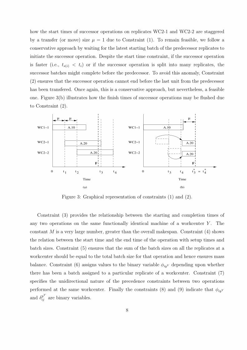
how the start times of successor operations on replicates WC2-1 and WC2-2 are staggered

by a transfer (or move) size µ = 1 due to Constraint (1). To remain feasible, we follow a

conservative approach by waiting for the latest starting batch of the predecessor replicates to

initiate the successor operation. Despite the start time constraint, if the successor operation

is faster (i.e., ts(i) < ti) or if the successor operation is split into many replicates, the

successor batches might complete before the predecessor. To avoid this anomaly, Constraint

(2) ensures that the successor operation cannot end before the last unit from the predecessor

has been transfered. Once again, this is a conservative approach, but nevertheless, a feasible

one. Figure 3(b) illustrates how the finish times of successor operations may be flushed due

to Constraint (2).

WC1−1

WC2−1

WC2−2

A.10

µ µ

WC2−1

WC1−1

WC2−2

Time

(b)(a)

FF

= **

A.20

A.20

µ

A.20

A.20

A.10

00

Time

4t3t3t 4t4t3t2t1t

Figure 3: Graphical representation of constraints (1) and (2).

Constraint (3) provides the relationship between the starting and completion times of

any two operations on the same functionally identical machine of a workcenter Y . The

constant M is a very large number, greater than the overall makespan. Constraint (4) shows

the relation between the start time and the end time of the operation with setup times and

batch sizes. Constraint (5) ensures that the sum of the batch sizes on all the replicates at a

workcenter should be equal to the total batch size for that operation and hence ensures mass

balance. Constraint (6) assigns values to the binary variable φiyY depending upon whether

there has been a batch assigned to a particular replicate of a workcenter. Constraint (7)

specifies the unidirectional nature of the precedence constraints between two operations

performed at the same workcenter. Finally the constraints (8) and (9) indicate that φiyY

and δyY

ij are binary variables.

8

3.3 Mathematical Model With Batch Splitting and Movesize

To avoid excessive material handling costs, or for the purpose of unitizing, often a minimum

movesize is established. The movesize µ is defined as the threshold size (quantity) for an

operation that needs to be processed before it can be transferred for the successor operation.

In this section we discuss how to revise the BSAS problem to incorporate movesize along

with batch splitting. The BSAS problem with movesize (BSASM) is developed and the

resulting problem (P1) is defined as:

Minimize : Max {Fz}

z∈E

Subject to:

Ss(i)yY ′ ≥ SiyY + KiφiyY − Ks(i)φs(i)yY ′ + µ

yY′

∑

y=1

φs(i)y

ti

∀s(i) ∈ IY ′ , ∀i ∈ IY ,∀yY , yY ′

, ∀Y, Y ′, Y 6= Y ′ (10)

Fs(i)yY ′ ≥ FiyY + µts(i) ∀s(i) ∈ IY ′ , ∀i ∈ IY ,∀yY , yY ′

, ∀Y, Y ′, Y 6= Y ′ (11)

(3), (4), (5), (6), (7), (8), and (9).

As before, the objective function minimizes the production makespan. Constraints (10)

and (11) are similar to the constraints (1) and (2), respectively, except that they incorporate

the movesize µ in the determination of start and finish times.

3.4 Illustrative Example

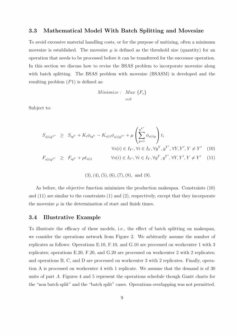
To illustrate the efficacy of these models, i.e., the effect of batch splitting on makespan,

we consider the operations network from Figure 2. We arbitrarily assume the number of

replicates as follows: Operations E.10, F.10, and G.10 are processed on workcenter 1 with 3

replicates; operations E.20, F.20, and G.20 are processed on workcenter 2 with 2 replicates;

and operations B, C, and D are processed on workcenter 3 with 2 replicates. Finally, opera-

tion A is processed on workcenter 4 with 1 replicate. We assume that the demand is of 30

units of part A. Figures 4 and 5 represent the operations schedule though Gantt charts for

the “non batch split” and the “batch split” cases. Operations overlapping was not permitted.

9

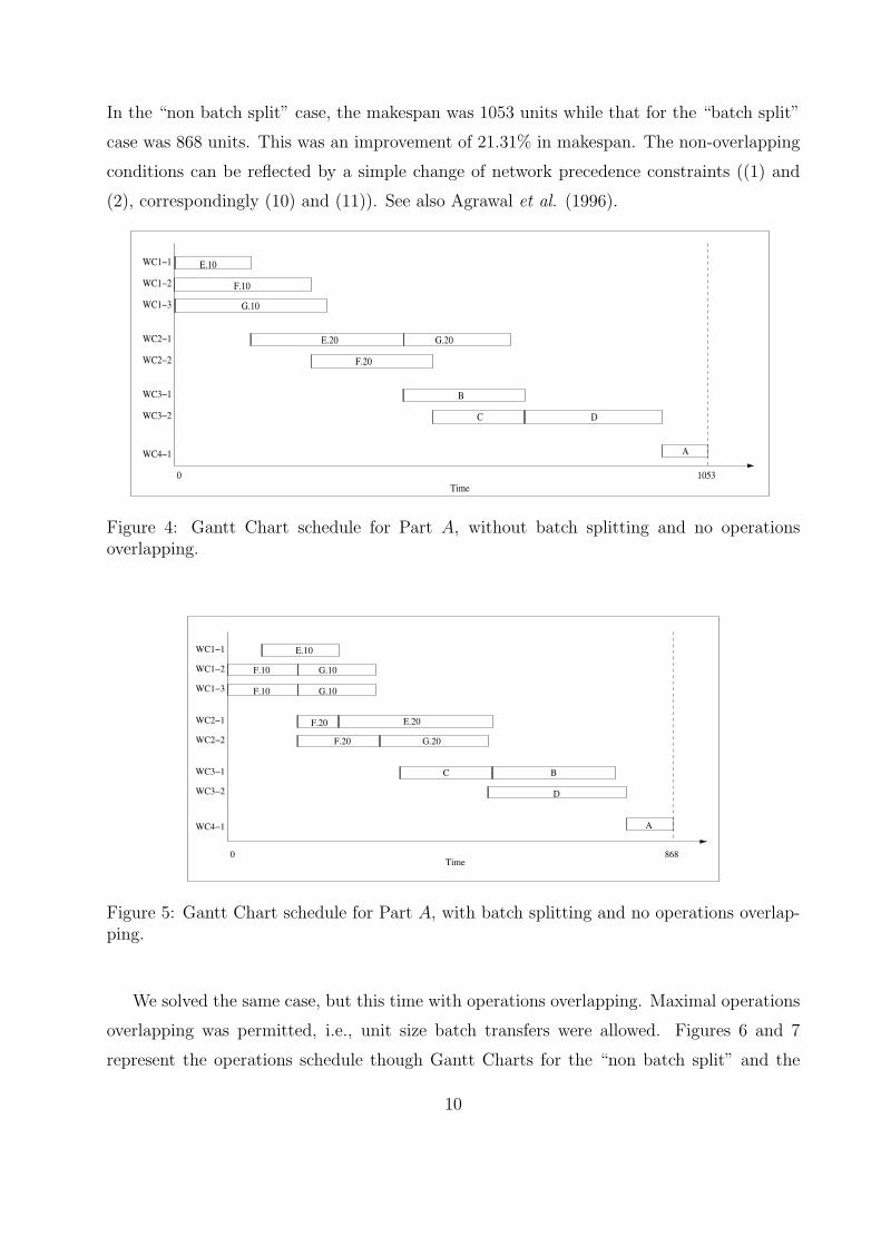
In the “non batch split” case, the makespan was 1053 units while that for the “batch split”

case was 868 units. This was an improvement of 21.31% in makespan. The non-overlapping

conditions can be reflected by a simple change of network precedence constraints ((1) and

(2), correspondingly (10) and (11)). See also Agrawal et al. (1996).

E.10

F.10

G.10

WC1−1

WC1−2

WC1−3

WC2−1

WC2−2

WC3−1

WC3−2

0

WC4−1

Time

G.20

F.20

1053

E.20

B

C D

A

Figure 4: Gantt Chart schedule for Part A, without batch splitting and no operationsoverlapping.

WC1−1

WC1−2

WC1−3

WC2−1

WC2−2

WC3−1

WC3−2

F.10 G.10

G.10F.10

0Time

F.20

WC4−1

E.10

868

A

B

D

G.20

E.20

C

F.20

Figure 5: Gantt Chart schedule for Part A, with batch splitting and no operations overlap-ping.

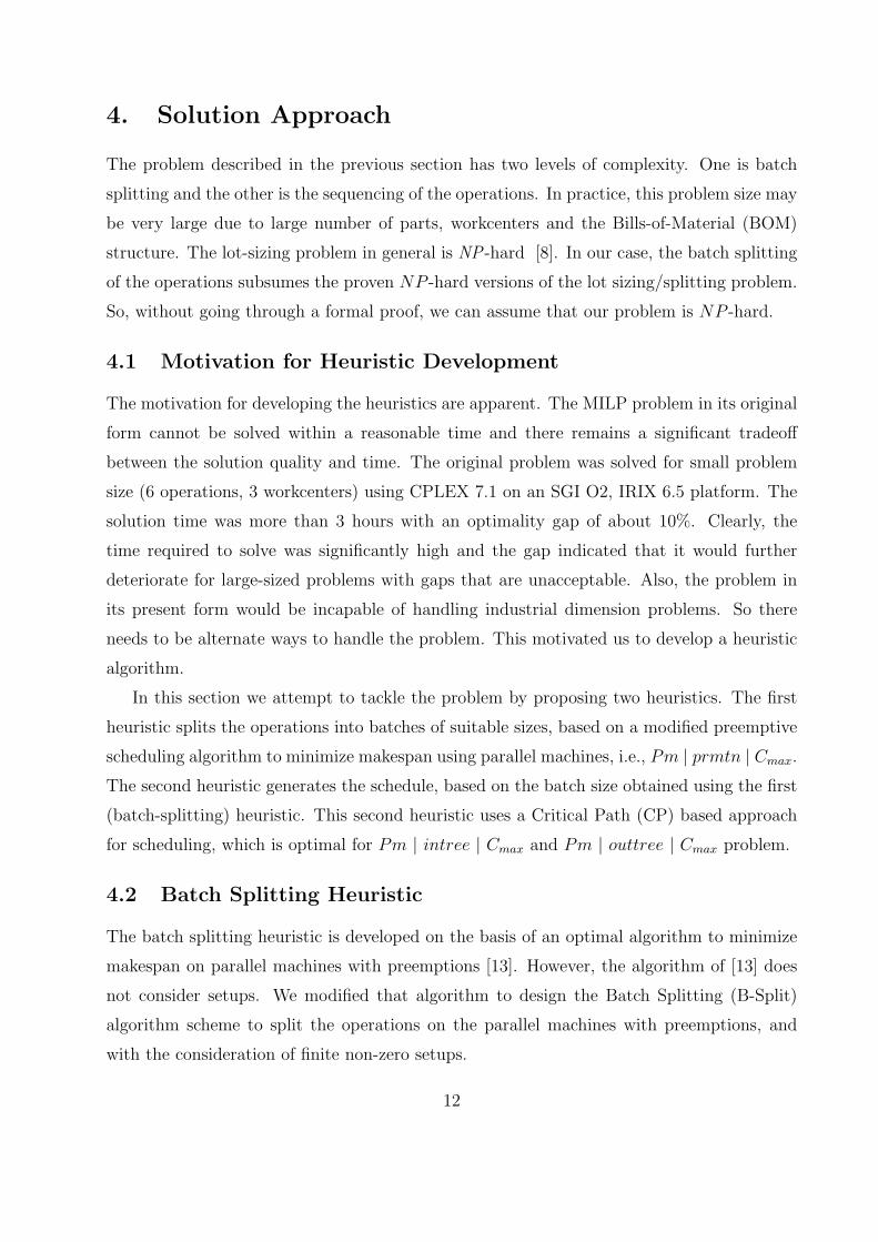
We solved the same case, but this time with operations overlapping. Maximal operations

overlapping was permitted, i.e., unit size batch transfers were allowed. Figures 6 and 7

represent the operations schedule though Gantt Charts for the “non batch split” and the

10

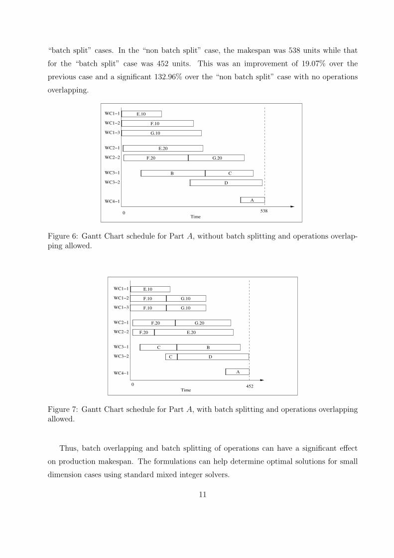
“batch split” cases. In the “non batch split” case, the makespan was 538 units while that

for the “batch split” case was 452 units. This was an improvement of 19.07% over the

previous case and a significant 132.96% over the “non batch split” case with no operations

overlapping.

WC1−1

WC1−2

WC1−3

WC2−1

WC2−2

WC3−1

WC3−2

F.10

G.10

F.20

0

WC4−1

G.20

Time

538

A

D

CB

E.20

E.10

Figure 6: Gantt Chart schedule for Part A, without batch splitting and operations overlap-ping allowed.

WC1−1

WC1−2

WC1−3

WC2−1

WC2−2

WC3−1

WC3−2

E.10

F.10

F.10

WC4−1

0

B

Time

F.20 G.20

D

F.20 E.20

G.10

G.10

452

A

C

C

Figure 7: Gantt Chart schedule for Part A, with batch splitting and operations overlappingallowed.

Thus, batch overlapping and batch splitting of operations can have a significant effect

on production makespan. The formulations can help determine optimal solutions for small

dimension cases using standard mixed integer solvers.

11

4. Solution Approach

The problem described in the previous section has two levels of complexity. One is batch

splitting and the other is the sequencing of the operations. In practice, this problem size may

be very large due to large number of parts, workcenters and the Bills-of-Material (BOM)

structure. The lot-sizing problem in general is NP -hard [8]. In our case, the batch splitting

of the operations subsumes the proven NP -hard versions of the lot sizing/splitting problem.

So, without going through a formal proof, we can assume that our problem is NP -hard.

4.1 Motivation for Heuristic Development

The motivation for developing the heuristics are apparent. The MILP problem in its original

form cannot be solved within a reasonable time and there remains a significant tradeoff

between the solution quality and time. The original problem was solved for small problem

size (6 operations, 3 workcenters) using CPLEX 7.1 on an SGI O2, IRIX 6.5 platform. The

solution time was more than 3 hours with an optimality gap of about 10%. Clearly, the

time required to solve was significantly high and the gap indicated that it would further

deteriorate for large-sized problems with gaps that are unacceptable. Also, the problem in

its present form would be incapable of handling industrial dimension problems. So there

needs to be alternate ways to handle the problem. This motivated us to develop a heuristic

algorithm.

In this section we attempt to tackle the problem by proposing two heuristics. The first

heuristic splits the operations into batches of suitable sizes, based on a modified preemptive

scheduling algorithm to minimize makespan using parallel machines, i.e., Pm | prmtn | Cmax.

The second heuristic generates the schedule, based on the batch size obtained using the first

(batch-splitting) heuristic. This second heuristic uses a Critical Path (CP) based approach

for scheduling, which is optimal for Pm | intree | Cmax and Pm | outtree | Cmax problem.

4.2 Batch Splitting Heuristic

The batch splitting heuristic is developed on the basis of an optimal algorithm to minimize

makespan on parallel machines with preemptions [13]. However, the algorithm of [13] does

not consider setups. We modified that algorithm to design the Batch Splitting (B-Split)

algorithm scheme to split the operations on the parallel machines with preemptions, and

with the consideration of finite non-zero setups.

12

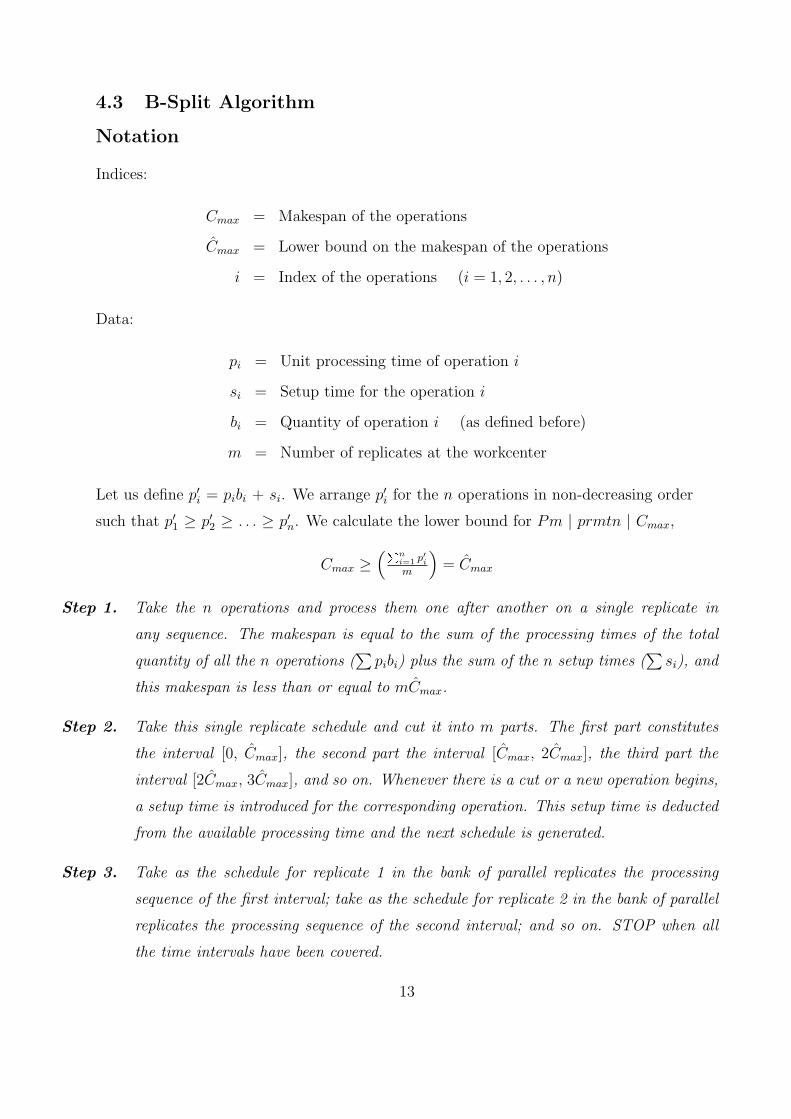
4.3 B-Split Algorithm

Notation

Indices:

Cmax = Makespan of the operations

Cmax = Lower bound on the makespan of the operations

i = Index of the operations (i = 1, 2, . . . , n)

Data:

pi = Unit processing time of operation i

si = Setup time for the operation i

bi = Quantity of operation i (as defined before)

m = Number of replicates at the workcenter

Let us define p′i = pibi + si. We arrange p′i for the n operations in non-decreasing order

such that p′1 ≥ p′2 ≥ . . . ≥ p′n. We calculate the lower bound for Pm | prmtn | Cmax,

Cmax ≥(P

n

i=1p′

i

m

)

= Cmax

Step 1. Take the n operations and process them one after another on a single replicate in

any sequence. The makespan is equal to the sum of the processing times of the total

quantity of all the n operations (∑

pibi) plus the sum of the n setup times (∑

si), and

this makespan is less than or equal to mCmax.

Step 2. Take this single replicate schedule and cut it into m parts. The first part constitutes

the interval [0, Cmax], the second part the interval [Cmax, 2Cmax], the third part the

interval [2Cmax, 3Cmax], and so on. Whenever there is a cut or a new operation begins,

a setup time is introduced for the corresponding operation. This setup time is deducted

from the available processing time and the next schedule is generated.

Step 3. Take as the schedule for replicate 1 in the bank of parallel replicates the processing

sequence of the first interval; take as the schedule for replicate 2 in the bank of parallel

replicates the processing sequence of the second interval; and so on. STOP when all

the time intervals have been covered.

13

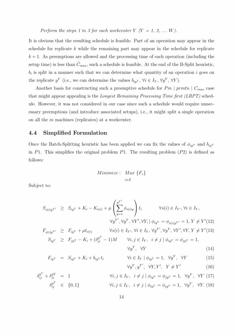
Perform the steps 1 to 3 for each workcenter Y (Y = 1, 2, . . . W ).

It is obvious that the resulting schedule is feasible. Part of an operation may appear in the

schedule for replicate k while the remaining part may appear in the schedule for replicate

k + 1. As preemptions are allowed and the processing time of each operation (including the

setup time) is less than Cmax, such a schedule is feasible. At the end of the B-Split heuristic,

bi is split in a manner such that we can determine what quantity of an operation i goes on

the replicate yY (i.e., we can determine the values biyY , ∀i ∈ IY , ∀yY , ∀Y ).

Another basis for constructing such a preemptive schedule for Pm | prmtn | Cmax case

that might appear appealing is the Longest Remaining Processing Time first (LRPT) sched-

ule. However, it was not considered in our case since such a schedule would require unnec-

essary preemptions (and introduce associated setups), i.e., it might split a single operation

on all the m machines (replicates) at a workcenter.

4.4 Simplified Formulation

Once the Batch-Splitting heuristic has been applied we can fix the values of φiyY and biyY

in P1. This simplifies the original problem P1. The resulting problem (P2) is defined as

follows:

Minimize : Max {Fz}

z∈E

Subject to:

Ss(i)yY ′ ≥ SiyY + Ki − Ks(i) + µ

yY′

∑

y=1

φs(i)y

ti ∀s(i) ∈ IY ′ , ∀i ∈ IY ,

∀yY ′

,∀yY , ∀Y ′,∀Y, | φiyY = φs(i)yY ′ = 1, Y 6= Y ′(12)

Fs(i)yY ′ ≥ FiyY + µts(i) ∀s(i) ∈ IY ′ , ∀i ∈ IY , ∀yY ′

,∀yY , ∀Y ′,∀Y, Y 6= Y ′(13)

SiyY ≥ FjyY − Ki + (δyY

ji − 1)M ∀i, j ∈ IY , i 6= j | φiyY = φjyY = 1,

∀yY , ∀Y (14)

FiyY = SiyY + Ki + biyY ti ∀i ∈ IY | φiyY = 1, ∀yY , ∀Y (15)

∀yY , yY ′

, ∀Y, Y ′, Y 6= Y ′ (16)

δyY

ij + δyYji = 1 ∀i, j ∈ IY , i 6= j | φiyY = φjyY = 1, ∀yY , ∀Y (17)

δyY

ij ∈ {0, 1} ∀i, j ∈ IY , i 6= j | φiyY = φjyY = 1, ∀yY , ∀Y. (18)

14

This is a much simpler formulation that P1. The objective function minimizes the production

makespan. Constraints (12), (13), (14), (15), (17), and (18) have the same significance as

constraints (10), (11), (3), (4), (7), and (9) respectively. The computational results in Section

5 indicate that P2 takes significantly less computational time than P1 and P .

4.5 Batch Scheduling Heuristic

The Batch-Splitting heuristic fixes the values of φiyY and biyY and generates a much sim-

pler formulation P2. However, the binary variables δyY

ij still make P2 intractable for large

industrial-sized problems. The Batch Scheduling heuristic determines the schedule based on

the results obtained from the Batch-Splitting heuristic. We develop the (B-Sched) algorithm

to incorporate this heuristic.

4.6 B-Sched Algorithm

The Critical Path approach is optimal for Pm | intree | Cmax and Pm | outtree | Cmax (See

Pinedo, 2002). The operations network generated after applying the B-Split algorithm is

equivalent to Pm | tree | Cmax. This critical path based procedure has shown to provide

good results for different versions of the assembly scheduling problem (see, Agrawal et al.,

1996, Anwar and Nagi, 1997, 1998). We developed the B-Sched algorithm based on the

Critical Path approach to schedule the operations. The algorithm is presented as follows:

Step 1. Do a “forward pass” in an uncapacitated sense to determine the Early Finish times of

the operations such that the network constraints (12) and (13) are satisfied.

Step 3. Sort the operations according to the ascending order of the Early Finish times at the

final node (set of end operations).

Step 4. Set the finish times of all the end operations (z ∈ E) to the Early Finish time of the

latest end operations (i.e., the Early Finish time of the entire network).

Step 5. Do a “backward pass” in a capacitated sense to determine the final schedule such that

the constraints (12), (13) and (14) are satisfied. STOP.

The “forward pass” method used here is exactly the same as that used in the Critical Path

Method (CPM) [14]. The critical path of the operations network represents the time required

for the completion of the latest finishing operation in the network assuming infinite resources.

15

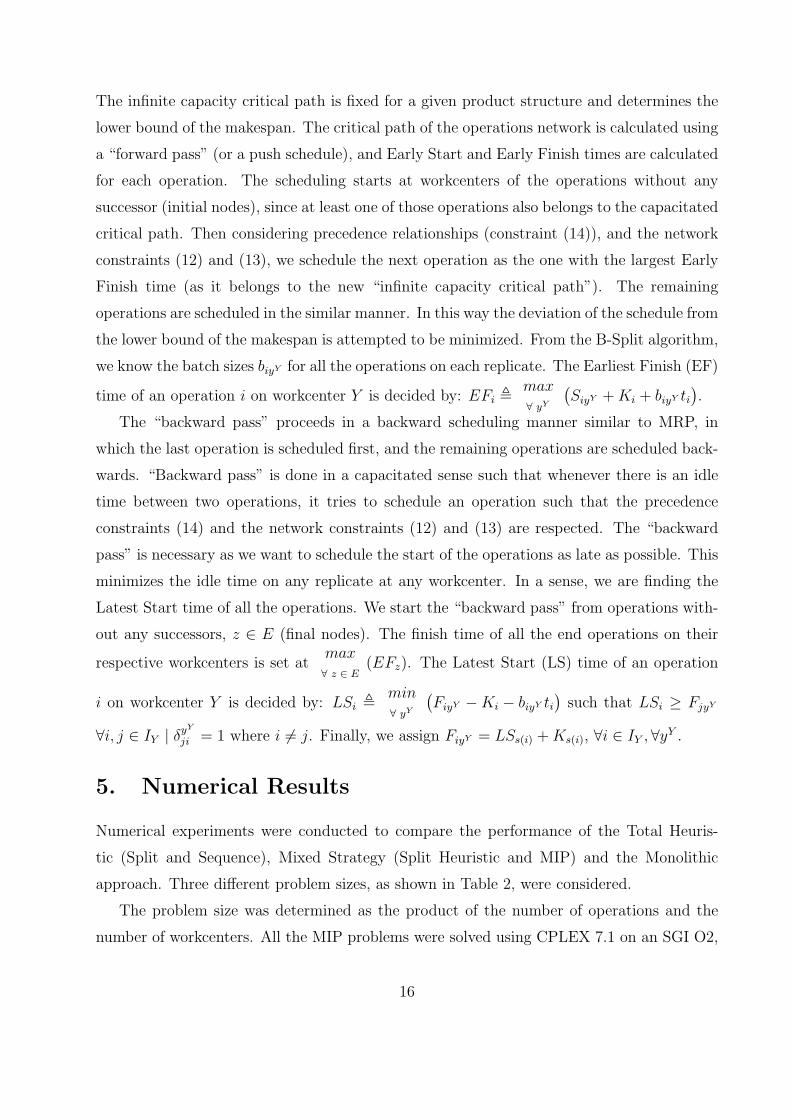
The infinite capacity critical path is fixed for a given product structure and determines the

lower bound of the makespan. The critical path of the operations network is calculated using

a “forward pass” (or a push schedule), and Early Start and Early Finish times are calculated

for each operation. The scheduling starts at workcenters of the operations without any

successor (initial nodes), since at least one of those operations also belongs to the capacitated

critical path. Then considering precedence relationships (constraint (14)), and the network

constraints (12) and (13), we schedule the next operation as the one with the largest Early

Finish time (as it belongs to the new “infinite capacity critical path”). The remaining

operations are scheduled in the similar manner. In this way the deviation of the schedule from

the lower bound of the makespan is attempted to be minimized. From the B-Split algorithm,

we know the batch sizes biyY for all the operations on each replicate. The Earliest Finish (EF)

time of an operation i on workcenter Y is decided by: EFi ,max

∀ yY

(

SiyY + Ki + biyY ti)

.

The “backward pass” proceeds in a backward scheduling manner similar to MRP, in

which the last operation is scheduled first, and the remaining operations are scheduled back-

wards. “Backward pass” is done in a capacitated sense such that whenever there is an idle

time between two operations, it tries to schedule an operation such that the precedence

constraints (14) and the network constraints (12) and (13) are respected. The “backward

pass” is necessary as we want to schedule the start of the operations as late as possible. This

minimizes the idle time on any replicate at any workcenter. In a sense, we are finding the

Latest Start time of all the operations. We start the “backward pass” from operations with-

out any successors, z ∈ E (final nodes). The finish time of all the end operations on their

respective workcenters is set atmax

∀ z ∈ E(EFz). The Latest Start (LS) time of an operation

i on workcenter Y is decided by: LSi ,min

∀ yY

(

FiyY − Ki − biyY ti)

such that LSi ≥ FjyY

∀i, j ∈ IY | δyY

ji = 1 where i 6= j. Finally, we assign FiyY = LSs(i) + Ks(i), ∀i ∈ IY ,∀yY .

5. Numerical Results

Numerical experiments were conducted to compare the performance of the Total Heuris-

tic (Split and Sequence), Mixed Strategy (Split Heuristic and MIP) and the Monolithic

approach. Three different problem sizes, as shown in Table 2, were considered.

The problem size was determined as the product of the number of operations and the

number of workcenters. All the MIP problems were solved using CPLEX 7.1 on an SGI O2,

16

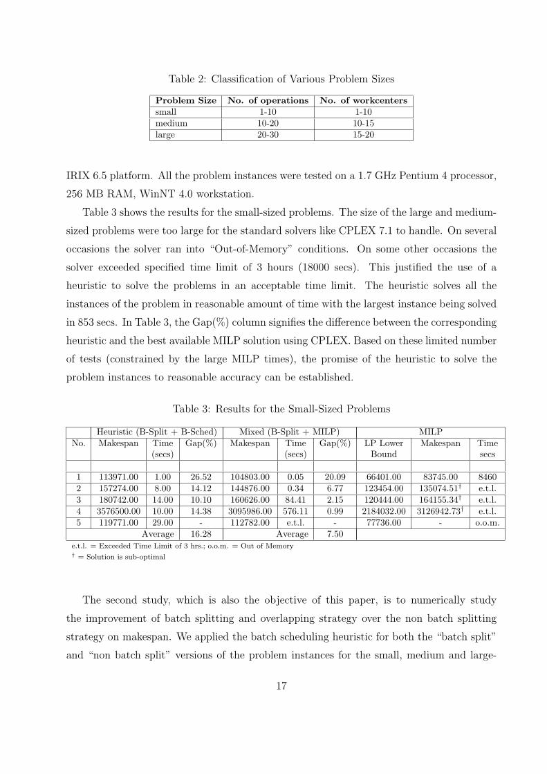
Table 2: Classification of Various Problem Sizes

Problem Size No. of operations No. of workcenters

small 1-10 1-10medium 10-20 10-15large 20-30 15-20

IRIX 6.5 platform. All the problem instances were tested on a 1.7 GHz Pentium 4 processor,

256 MB RAM, WinNT 4.0 workstation.

Table 3 shows the results for the small-sized problems. The size of the large and medium-

sized problems were too large for the standard solvers like CPLEX 7.1 to handle. On several

occasions the solver ran into “Out-of-Memory” conditions. On some other occasions the

solver exceeded specified time limit of 3 hours (18000 secs). This justified the use of a

heuristic to solve the problems in an acceptable time limit. The heuristic solves all the

instances of the problem in reasonable amount of time with the largest instance being solved

in 853 secs. In Table 3, the Gap(%) column signifies the difference between the corresponding

heuristic and the best available MILP solution using CPLEX. Based on these limited number

of tests (constrained by the large MILP times), the promise of the heuristic to solve the

problem instances to reasonable accuracy can be established.

Table 3: Results for the Small-Sized Problems

Heuristic (B-Split + B-Sched) Mixed (B-Split + MILP) MILPNo. Makespan Time Gap(%) Makespan Time Gap(%) LP Lower Makespan Time

(secs) (secs) Bound secs

1 113971.00 1.00 26.52 104803.00 0.05 20.09 66401.00 83745.00 84602 157274.00 8.00 14.12 144876.00 0.34 6.77 123454.00 135074.51† e.t.l.3 180742.00 14.00 10.10 160626.00 84.41 2.15 120444.00 164155.34† e.t.l.4 3576500.00 10.00 14.38 3095986.00 576.11 0.99 2184032.00 3126942.73† e.t.l.5 119771.00 29.00 - 112782.00 e.t.l. - 77736.00 - o.o.m.

Average 16.28 Average 7.50e.t.l. = Exceeded Time Limit of 3 hrs.; o.o.m. = Out of Memory† = Solution is sub-optimal

The second study, which is also the objective of this paper, is to numerically study

the improvement of batch splitting and overlapping strategy over the non batch splitting

strategy on makespan. We applied the batch scheduling heuristic for both the “batch split”

and “non batch split” versions of the problem instances for the small, medium and large-

17

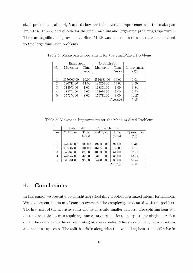
sized problems. Tables 4, 5 and 6 show that the average improvements in the makespan

are 5.15%, 16.22% and 21.80% for the small, medium and large-sized problems, respectively.

These are significant improvements. Since MILP was not used in these tests, we could afford

to test large dimension problems.

Table 4: Makespan Improvement for the Small-Sized Problems

Batch Split No Batch SplitNo. Makespan Time Makespan Time Improvement

(secs) (secs) (%)

1 3576500.00 10.00 3576681.00 10.00 0.012 180742.00 14.00 185254.00 14.00 2.503 113971.00 1.00 118351.00 1.00 3.844 119771.00 9.00 128074.00 9.00 6.935 157274.00 8.00 179711.00 8.00 14.27

Average 5.15

Table 5: Makespan Improvement for the Medium Sized Problems

Batch Split No Batch SplitNo. Makespan Time Makespan Time Improvement

(secs) (secs) (%)

1 454365.00 108.00 492102.00 92.00 8.312 418807.00 101.00 461340.00 102.00 10.163 358438.00 83.00 403163.00 51.00 12.484 752557.00 32.00 931210.00 33.00 23.745 667931.00 93.00 844405.00 80.00 26.42

Average 16.22

6. Conclusions

In this paper, we present a batch splitting scheduling problem as a mixed integer formulation.

We also present heuristic schemes to overcome the complexity associated with the problem.

The first part of the heuristic splits the batches into smaller batches. The splitting heuristic

does not split the batches requiring unnecessary preemptions, i.e., splitting a single operation

on all the available machines (replicates) at a workcenter. This automatically reduces setups

and hence setup costs. The split heuristic along with the scheduling heuristic is effective in

18

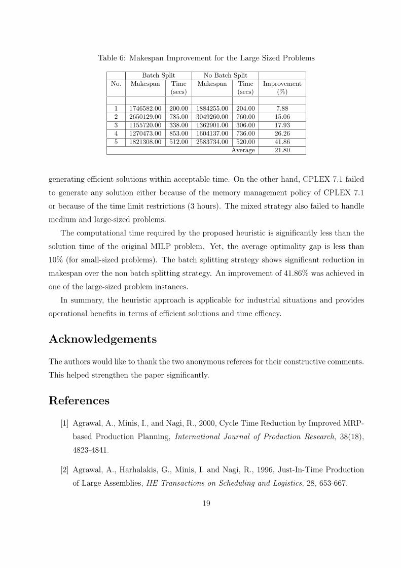
Table 6: Makespan Improvement for the Large Sized Problems

Batch Split No Batch SplitNo. Makespan Time Makespan Time Improvement

(secs) (secs) (%)

1 1746582.00 200.00 1884255.00 204.00 7.882 2650129.00 785.00 3049260.00 760.00 15.063 1155720.00 338.00 1362901.00 306.00 17.934 1270473.00 853.00 1604137.00 736.00 26.265 1821308.00 512.00 2583734.00 520.00 41.86

Average 21.80

generating efficient solutions within acceptable time. On the other hand, CPLEX 7.1 failed

to generate any solution either because of the memory management policy of CPLEX 7.1

or because of the time limit restrictions (3 hours). The mixed strategy also failed to handle

medium and large-sized problems.

The computational time required by the proposed heuristic is significantly less than the

solution time of the original MILP problem. Yet, the average optimality gap is less than

10% (for small-sized problems). The batch splitting strategy shows significant reduction in

makespan over the non batch splitting strategy. An improvement of 41.86% was achieved in

one of the large-sized problem instances.

In summary, the heuristic approach is applicable for industrial situations and provides

operational benefits in terms of efficient solutions and time efficacy.

Acknowledgements

The authors would like to thank the two anonymous referees for their constructive comments.

This helped strengthen the paper significantly.

References

[1] Agrawal, A., Minis, I., and Nagi, R., 2000, Cycle Time Reduction by Improved MRP-

based Production Planning, International Journal of Production Research, 38(18),

4823-4841.

[2] Agrawal, A., Harhalakis, G., Minis, I. and Nagi, R., 1996, Just-In-Time Production

of Large Assemblies, IIE Transactions on Scheduling and Logistics, 28, 653-667.

19

[3] Anwar, M.F. and Nagi, R., 1997, Integrated Lot-sizing and Scheduling for Just-In-

Time Production of Complex Assemblies with Finite Set-ups, International Journal

of Production Research, 35(5), 1447-1470.

[4] Anwar, M.F. and Nagi, R., 1998, Integrated Scheduling of Material Handling and

Manufacturing Activities for Just-In-Time Production of Complex Assemblies, Inter-

national Journal of Production Research, 36(3), 653-681.

[5] Baker, K.R., and Pyke, D.F., 1990, Solution Procedures for the Lot Streaming Prob-

lem, Decision Sciences, 21(3), 457-492.

[6] Botsali, A.R., 1999, Lot Streaming Techniques, Technical Note.

[7] Dauzere-Peres, S., and Lasserre, J.B., 1994, Integration of Planning and Scheduling

Decisions in a Job-Shop, European Journal of Operations Research, 75, 413-426.

[8] Florian, M., Lenstra, J.K., and Rinnooy Kan H.G., 1980, Deterministic Production

Planning: Algorithms and Complexity, Management Science, 26(7), 669-679.

[9] Graves, S.C., and Kostreva, M.M., 1986, Overlapping Operations in Material Re-

quirements Planning, Journal of Operations Management, 6(3), 283-294.

[10] Jacobs, F.R., and Bragg, D.J., 1988, Repetitive Lots: Flow-Time Reduction Through

Sequencing and Dynamic Batch Sizing, Decision Sciences, 19, 281-294.

[11] Kropp, D.H., and Smunt, T.L., 1990, Optimal and Heuristic Models for Lot Splitting

in a Flow Shop, Decision Sciences, 21, 691-709.

[12] Orlicky, J., 1975, Materials Requirement Planning, (McGraw Hill, NY).

[13] Pinedo, M., 2002, Scheduling: Theory, Algorithms, and Systems, 2nd ed., (Prentice

Hall, Englewood Cliffs, NJ), 106-107.

[14] Taha, H.A. 1996, Operations Research: An Introduction, 6th ed., (Prentice Hall,

Upper Saddle River, NJ).

[15] Trietsch, D., and Baker, K.R., 1993, Basic Techniques for Lot Streaming, Operations

Research, 41(6), 1065-1076.

20

[16] Wagner, B., and Ragatz, G., 1994, The Impact on Lot Splitting on Due Date Perfor-

mance, Journal of Operations Management, 12(1), 13-26.

[17] Yavuz, S., 1999, Scheduling with Batching and Lot-sizing, Bilkent University, Tech-

nical Note.

21