Battery Cell Temperature Estimation Model andCost Analysis of a Grid-Connected PV-BESS Plant

Md Mehedi Hasan∗, S. Ali Pourmousav† and Tapan K. Saha‡School of Information Technology and Electrical Engineering, The University of Queensland, Australia

Email: ∗mdmehedi.hasan@uq.edu.au, †a.pour@uq.edu.au, ‡saha@itee.uq.edu.au

Abstract—Battery cell temperature is an important factor inbattery capacity degradation, performance, and safety. Elevatedbattery cell temperature, due to intense battery operation withhigh charging-discharging current and ambient temperature,accelerates battery capacity degradation as well as causingextra cooling cost. Therefore, it is indispensable to estimatebattery cell temperature accurately for optimal BESS operationconsidering capacity degradation and its associated costs. Themain objectives of this paper are to propose a linear model toestimate battery cell temperature using Autoregressive IntegratedMoving Average with eXogenous variables (ARIMAX) consid-ering strongly correlated independent variables and propose acost function of PV plant with and without battery operation.The simulation results using field data show high accuracy ofthe proposed temperature estimation model without consideringthe complex thermal dynamics of the entire system. In addition,comprehensive cost functions are developed to show the benefitof integrating battery storage into a PV plant and determineinfluential factors to consider in any optimal battery operationsystems.

Index Terms—Battery cell temperature, degradation, ARI-MAX, cost analysis, PV plant, BESS

I. INTRODUCTION

With the growth of large-scale photovoltaic (PV) and windplants all over the world, the battery energy storage system(BESS) has become popular. BESS is essential for storingexcess renewable generation when it is available and utilising itefficiently and economically during peak hours. It also plays avital role in compensating the variability of renewable genera-tion [1]. While technological improvement and cost reductionof electrochemical storage devices are taking place, batterydegradation remains a big concern for the wide applicationof BESS [2]. To that end, an effective energy managementsystem (EMS) is needed to operate battery in an optimal wayby considering degradation and its associated costs. This canreduce unnecessary battery operation, which is responsible forhigher degradation. To design a reliable EMS, it is importantto derive a cost function for BESS operation considering allassociated costs such as degradation and cooling costs. It helpsto extend battery lifetime, which will economically benefit theentire system operation.

Battery capacity degrades due to charging-discharging op-erations as well as during idle condition [3], [4]. Amongvarious responsible factors for battery capacity degradation,battery cell temperature has a crucial impact on accelerat-ing battery capacity reduction [5]. In [6], it is shown that

every 10◦C battery cell temperature rise doubles the batterydegradation. Accumulated heat generated by large-scale BESSplaced in a confined container increases room temperature,which accelerates cooling system operation to keep the roomtemperature at an acceptable range. As a result, the elevatedbattery temperature increases operational cost for renewableplants with BESS. This way, it is essential to estimate batterytemperature evolution with respect to battery operation andambient temperature to have a better understanding of theincurred cost.

While a significant number of research studies has beenconducted on thermal management of battery in electric ve-hicles (EVs) and plug-in hybrid electric vehicles (PHEVs) byproposing general models of battery thermal behaviour [7],[8], no such research has been conducted using linear mod-elling approach to estimate thermal behaviour of utility-scaleBESS in connection with a grid-integrated renewable powerplant. Detailed thermodynamic modelling to determine thermalbehaviour of a single battery module is not feasible for large-scale BESS, where complex thermal interactions betweenthousands of battery cells are involved. This type of thermalmodelling with intensive measurements and computationalefforts, as suggested in [9], is not practicable for the EMS inutility-scale BESS because of the cost and scalability issues.Moreover, to the best of our knowledge, a comprehensive costfunction for utility-scale BESS, including influential factorssuch as battery capacity degradation, cooling system operationand battery operational costs related to BESS operation, hasnot been reported in the literature.

In this paper, a data-driven battery cell temperature esti-mation model is proposed for a 600kW/760kWh BESS in a3.275 MWp PV plant, located at the University of Queensland(UQ) Gatton campus, using a widely accepted linear statisticalforecasting method, ARIMAX [10], [11], [12], which canbe conveniently integrated with EMSs. A data-driven methoddoes not require the physical dynamics of the BESS andthermal interactions between effective parameters. Instead,only historical data is needed to estimate future battery celltemperature. In addition, the proposed cost function in thisstudy estimates total plant cost/benefit by considering batterycapacity degradation, cooling cost, imported/exported energyfrom/to the grid, exported PV energy to the grid based inFeed-in-Tariff (FiT), and demand charge. A linear degradationmodel is adapted to calculate battery ageing. A comparisonstudy has also been presented in this study to evaluate the total

1

cost of plant operation with and without BESS in a grid-tiedPV plant. Actual field data from the UQ PV-BESS plant is usedfor modelling and evaluating the proposed methodologies.Extensive simulation results show the high accuracy of theproposed temperature model and prove the necessity of suchmodels for optimal BESS operation.

The rest of the paper is organised as follows: Section IIpresents ARIMAX modelling for battery cell temperatureestimation. Section III explains the cost formulations of PVplant with and without BESS. Section IV presents simulationstudy based on field data. Finally, the paper is concluded inSection V and future work is outlined.

II. BATTERY CELL TEMPERATURE MODELLING

In this study, ARIMAX is used to estimate battery celltemperature as a linear model. It is a powerful tool to outlinethe dynamics of a time series. The ARIMAX concept isproposed over ARIMA as a multivariate method that caninclude independent variables, which are important in thebattery cell temperature model. In ARIMA, only dependentvariable is regressed on its own lagged values (i.e., AR terms),error values generated in previous time steps by the model (i.e.,MA terms) and the number of nonseasonal differences neededfor stationarity of time-series data. In addition to ARIMA,ARIMAX model takes the impact of exogenous variablesinto account. In this study, the charging-discharging currentof the battery and ambient temperature are considered as theexternal variables to estimate dependent variable, i.e., batterycell temperature, more accurately [3]. ARIMAX model can bemathematically represented as,yt = βxt +φ1yt-1 + ...+φpyt-p− θ1zt-1− · · · − θqzt-q + zt (1)

where yt represents dependent variable based on differencingof time series data; yt is the dependent variable denoting actualtime series; xt represents exogenous inputs at time t and β isthe coefficient of exogenous inputs; zt represents the forecasterrors; and φp and θq are the estimated coefficients of therespective variables. t denotes the time-step of the series.

The proposed model is classified as ARIMAX(p,d,q) model.There are three main parameters, namely p, d and q, to be setto determine the model. p is the number of auto-regressiveterms, d is the number of nonseasonal differences needed forconverting the non-stationary time-series to a stationary one,and q denotes the number of lagged forecast errors.

The identification of the model is performed in three steps.First step is to analyse the trend of time series to determinewhether transformation is needed. In order to check the sta-tionarity of the time series, statistical analysis will be carriedout. Two tests are used in this study to check the stationarityof the time series:

• Augmented dickey fuller (ADF) unit root testing is cho-sen to examines the null hypothesis of a unit root [13].

• KwiatkowskiPhillips-Schmidt-Shin (KPSS) test is uti-lized to determine the stationarity of a time series arounda mean or a linear trend [14].

Both tests collectively indicate the stationarity of a time serieswhen existence of a unit root is rejected by ADF test and the

mean/trend-stationarity of the time series is not rejected byKPSS test.

Second step is to find the best order of the auto-regressivemodel for estimating the battery cell temperature. An auto-regressive model predicts the dependent variable (i.e., batterycell temperature), where specific lagged values of the depen-dent variables are used as predictor variables. Partial autocor-relation function (PACF) is used to identify the order of theautorcorrelation or AR(p) model [15]. The other componentof ARIMAX is the moving average (MA) with the order of q.In a time series model, a moving average term is a past errormultiplied by a coefficient. Autocorrelation function (ACF)is used to determine the order (q) of MA model [15]. Thesemethods will be used in Section IV for modelling using actualdata.

Third step is to build the model using training dataset afteridentifying the p, d and q order. The coefficients of the modelare identified during the training process. The trained modelis then tested with a completely separate set of independentdata (called test data), which has not being used during thetraining process, to evaluate the performance of the model. Inorder to quantify the accuracy of the battery cell temperatureprediction, Root Mean Squared Error (RMSE), given in (2),is used as a standard measure.

RMSE =

√∑Ni=1 (Tai

− Tmi)2

N(2)

where Tai , Tmi and N represent time series of actual batterycell temperature, predicted battery cell temperature using ARI-MAX model, and the total number of samples, respectively.

III. COST FUNCTION DEVELOPMENT

A comprehensive cost assessment considering the mosteffective parameters is able to render an opportunity to de-velop a cost function for the entire plant. Dominant factorssuch as battery degradation cost due to cycling and calendarageing, cost of the cooling system, and the cost associatedwith charging-discharging operations of BESS have taken intoaccount to develop a complete cost function for the plant.Appropriate formulation is derived for plant operation costwith and without BESS for comparison purposes, which helpsto identify the effectiveness of the BESS integration in theplant. Such a comparison using simulation results will showthe necessity of optimally operating battery to avoid theunnecessary cost. In this study, we run our study on a PVplant. However, the same methodology can be used for otherrenewable-based plants.

A.PV plant cost with and without BESS

In this section, the plant operation costs with and without theBESS will be formulated step-by-step. The cost functions aredeveloped based on the UQ Gatton plant in Australia, whichhas a local grid-connected BESS of Li-Polymer batteries [16].The primary objectives of the plant are to fulfil campuselectricity requirements and reduce demand charge.

2

1)Total cost function with BESS: Although BESS is pri-marily integrated into the PV plant to store excess PV energyand utilise the energy when grid price is high, its continuousoperation in the plant causes extra cost. The dominant costfactors for operating a BESS are the cost associated withbattery degradation, cooling system operation, and importingpower from the grid to charge the BESS.

Fig. 1: Cost-benefit of the entire PV-BESS plant

Fig. 1 shows the daily cost-benefit associated with BESSoperation in the plant. Continuous battery operation in charg-ing and discharging modes as well as idle situation areresponsible for battery degradation. Moreover, elevated tem-perature created by battery cell and ambient temperature in theconfined BESS room accelerates the cooling system operationto maintain the room temperature within an acceptable range.Although a significant benefit is experienced by dischargingoperation of the BESS during peak hours, battery charging bythe grid and avoiding selling excess PV generation to the gridat FiT price (yellow area in Fig. 1) will add to the overall costof the system. As per operational rules, the BESS chargingfrom the grid only takes place during the off-peak time,when the price is relatively lower. In addition, BESS will becharged by the excess PV power, if available. Therefore, thisis considered as a cost in PV plant operation with BESS. Thetotal PV plant cost, i.e., CostWB, on a daily basis is calculatedusing Eq. (3), where the cost associated with dominant factorsare considered.CostWB = CostDailyDeg +CostDTC +CostDI +CostCFiT (3)

where CostDailyDeg refers to the total cost associated withdegradation; CostDTC and CostDI represent the cost of coolingsystem operation and imported grid-energy to charge theBESS, respectively. CostCFiT is the cost of charging the BESSwith excess PV energy in terms of opportunity loss to exportenergy to the grid at FiT rate.

Fig. 2: Cost-benefit of the PV plant without BESS

2)Total Cost of PV Plant Without BESS: PV plant withoutBESS is only able to export energy to the grid at FiT.

Due to unavailability of PV generation or storage duringevening peak, the plant is unable to reduce the peak demand.Consequently, the demand charge cost1 (shown in Fig. 2).Therefore, extra cost occurs for the PV plant without BESS.The total daily cost for PV plant without BESS, i.e., CostWOB,is estimated using Eq. (4).

CostWOB = CostDE + CostDC − FiTBenefit (4)where CostDE and CostDC are the cost of energy and demandcharge during peak hours, respectively. FiTBenefit refers to thebenefit from exporting PV energy to the grid.

B.Battery Degradation Cost

Degradation of a battery is a continuous process, whereseveral factors affect degradation at the same time. A batteryundergoes charge and discharge as well as idle situationthroughout its lifetime. Therefore, both processes (i.e., cyclingand calendar ageing processes) continuously drive batteryageing. A simplified linear cyclic and calendar ageing modelsare formulated in this study to quantify the degradation of theBESS. Accordingly, a cost function is developed to quantifythe cost of degradation on a daily basis. The hourly degrada-tion cost is calculated using Eq. (5).

CostDEG = CostBESS × (DEGCyclic +DEGCalendar) (5)where CostDEG presents the total degradation cost;DEGCyclic and DEGCalendar represent the degradationof BESS because of cyclic and calendar ageingmechanisms, respectively. The total cost of BESS iscalculated considering energy and power costs, i.e.,CostBESS = CkWh($)× Ecap(kWh) + CkW($)× Pcap(kW ).Here, the BESS rated power and energy capacity is representedby Ecap(kWh) and Pcap(kW ), respectively and prices perkWh and kW are denoted by CkWh and CkW.

1)Cyclic Ageing: Degradation of a battery for cyclic ageingmechanism during a specific time is quantified with respect tothe energy throughput for that time interval, and the entireenergy throughput of the BESS throughout its lifetime, givenin DEGCyclic = ETh/BLT. Here, ETh and BLT are represent-ing the total energy throughput for a given time interval andthe total BESS energy throughput until it reaches its end oflife (EoL), respectively. Charging and discharging activitiesof BESS are observed using Eq. (6) for each time-interval toquantify the energy throughput.

ETh = ηCH

t∑j=1

Pj,CH × h+ ηDCH

t∑j=1

| Pj,DCH | ×h (6)

where ETh is the total energy throughput; ηCH and ηDCH rep-resent the efficiency of charging and discharging operations,respectively; and Pj,CH and Pj,DCH are the real power in kWfor charging and discharging operations, respectively. Totalenergy throughput of the BESS is calculated using Eq. (7),which considers the battery’s EoL, total rated cycle number

1It is the cost of a single monthly peak demand that should be paid alongsideenergy cost. It is calculated by averaging the measured instantaneous powerin pre-defined intervals.

3

at the rated depth of discharge (DoD), and the rated energycapacity of the BESS.

BLT = 2×DoDR×ηCH

ηDCH×Ecap×

NR∑j=0

(1+EoL− 1

NR×j) (7)

where BLT is the total kWh throughput energy of the batteryover its lifetime. DoDR represents the rated DoD for theBESS; Ecap is the actual energy capacity of the BESS at thebeginning of its operation in the field; and NR is the ratedbattery cycles.

2)Calendar Ageing: Calendar ageing is estimated by count-ing the number of idle hours experienced by the BESS and thetotal calendar life of the battery, as given in DEGCalendar =TIdle/TLife. Here, TIdle and TLife are the time in which batteryis idle within a specific period of time and the entire calendarlife of the BESS, respectively. Hourly idle time during a dayis calculated using, TIdle =

∑tj=1 Sj × h. Here, Sj is the

ON/OFF status of the battery; TIdle represents the accumulatedidle time of the battery until time t. The status of the batteryis counted and accumulated for a certain period of time as perrequirement. The battery is considered OFF when Pj,CH = 0and Pj,DCH = 0 at a given time. Otherwise, battery is underoperation, i.e., ON.

The total battery calendar life is calculated using TLife =365 × 24 × TRATED, where TRATED is the rated calendarlife of the battery in year. Hourly quantified degradationachieved from the aforementioned equations is calculated ona daily basis by observing degradation for 24 hours. Thetotal degradation cost on daily basis can be calculated as:CostDailyDeg(t) =

∑24j=1 CostDEG,j .

C.Cooling Cost

The active cooling system at the UQ Gatton plant consistsof rack fans and air-conditioning unit with 7.7kW coolingcapacity, which is dedicated to keeping the confined storageroom temperature at an acceptable range. 85% of power isconsumed by compressor unit rated at 2.3kW, compared tothe condenser-evaporator fans rated at 0.43kW. The powerconsumption by rack fans is 0.36kW.

Operation of each cooling unit is controlled by certainrules, given in Eq. (8), which shows the type of operationin different thermal conditions. Minute-by-minute temperaturevalues are considered to calculate the total energy consumptionand associated cost by the cooling systems.

CCool(T ) =

CF , TR < 23◦C

CCOM + CF , TR ≥ 23◦C

CCOM + CF + CRF , (TC ≥ 29◦C) ∧ (TR ≥ 23◦C)

CF + CRF , (TC ≥ 29◦C) ∧ (TR < 23◦C)(8)

where CCool represents the hourly cooling cost; TR and TCrefer to the battery room temperature and average battery celltemperature, respectively. CCOM, CF and CRF are the costfunction of each cooling systems’ component, namely com-pressor, fan of air-conditioning unit, and rack fans on top ofeach battery bank, respectively. Daily cooling cost is calculatedusing CostDTC =

∑t=24n=1 CCool(n), where CostDTC refers to

the total daily energy cost of cooling system operation. Due to

different energy tariff during a day, shown in (9), hourly costis calculated using hourly energy consumption, by differentcooling system units.

τ(t) =

{6.545¢/kWh, t ∈ [11PM, 12AM), (12AM, 7AM ]

11.78¢/kWh, t ∈ [7AM, 11PM ](9)

where τ(t) represents the local time-of-use (TOU) tariffthroughout a day.D.Demand Charge

The demand charge is calculated based on the maxi-mum apparent power (kVA). kVA is calculated for each30 minutes period using, kVA =

√(kW)2 + (kVAr)2. The

maximum kVA demand is estimated for each billing period(30 days). Therefore, the recorded peak value is used forthe entire month’s demand charge calculation, CostMDC =kVAMaximum× (σDUoS +σTUoS), where CostMDC represents thedemand charge for monthly billing period; σDUoS and σTUoSdenote distribution use of system (DUoS) and transmission useof system (TUoS) charges (σDUoS = $12.49/kV A/month andσTUoS = $1.169/kV A/month) per month, respectively.

As demand charge is calculated based on 30-day period,daily demand charge cost, i.e., CostDC, is calculated bymultiplying the cost of demand charge per kVA per monthby the peak monthly power demand.E.Cost of imported energy from the grid and demand charge

CostDI =∑5

n=1EC(t) × τ(t) is utilised to calculatethe daily cost associated with the grid imported energy forcharging the BESS. Here, CostDI is the total daily cost ofimported energy from the grid. Hourly imported grid energy isrepresented by EC. The BESS is charged by the grid between1st and 5th hours of each day.

The BESS is playing a vital role by reducing peak loadduring discharging. In the absence of the BESS, PV plant willneed to buy the energy from the grid with the peak-periodtariff. The cost associated with the energy is calculated usingCostDE =

∑23n=18ED(t)× τ(t), where CostDE represents the

total daily cost of energy that is purchased from the grid duringpeak demand. The BESS is discharged between 18th and 23th

hours of each day for peak shaving, when the grid energy costis more and peak demand is more prone to happen. The hourlyenergy by discharging the BESS is represented by ED.F.FiT Benefit

The benefit obtained by the FiT scheme is calculated basedon the PV generated energy that is exported to the grid.The cost of charging the BESS with PV energy, CostCFitis calculated using CostCFiT(t) = PCPV(t) × h × ξFiT andFiTBenefit(t) = PEPV(t) × h × ξFiT is used to find out thecost of the exported PV energy. Here, PCPV and PEPV are thePV generated power for charging and exporting to the grid,respectively; and ξFiT = 2.356¢/kWh refers to FiT rate.

IV. SIMULATION STUDY

In this study, a significant number of data, that coversnumerous plausible combinations of charging-discharging and

4

ambient temperature operations, is used to establish the batterycell temperature model and cost analysis for the PV plant.◦ Data Selection for ARIMAX Model:

• To train the ARIMAX model, 12 months equivalent datawith 1-minute sampling rate from 1st April 2016 to31st March 2017 have been selected, which consists of516,960 samples (359 days).

• To evaluate the ARIMAX model, a separate 30 days oftest data is used from 1st April 2017 to 31st October 2017.

◦ Data Selection for Cost Analysis:• 13 months data, sampled every 1 minute, from 1st April

2016 to 30th September 2017 have been selected for thispurpose. Also, 13 days of data with seasonal differencesare selected to assess seasonality impact on the PV plant.

• 1 day with the highest peak demand from each billingperiod is selected for demand charge calculation for theentire billing period.

A.ARIMAX Estimation Model OutcomesAs mentioned in section II, PACF, ADF-KPSS and ACF

tests are used to find the best order of p, d and q, respectively,prior to modelling.

Stationarity of the time series is checked using ADF andKPSS tests. The p-value was about zero, which is far below0.05 (for 95% confidence interval). It gives the indication ofrejecting the null hypothesis, that is not having a unit root inthe time series. In addition, KPSS test fails to reject the nullhypothesis with a p-value less than 0.01 and test critical valuesof 0.347, 0.462 and 0.744 for 10%, 5% and 1% confidenceintervals, respectively. The test critical values are more thanthe test statistic value, 0.0733. Therefore, it can be concludedthat the time series data is stationary; hence, differencing thetime series data is not required. Therefore, the order of I(d)will be 0 or I(0).

-1-0.5

0 0.5

1

0 10 20 30 40 50 60

lag

ACF for AvgTemperature_B1_R1

+- 1.96/T^0.5

-1-0.5

0 0.5

1

0 10 20 30 40 50 60

Lag

PACF for AvgTemperature_B1_R1

+- 1.96/T^0.5

-0.5

PACF

Fig. 3: PACF plot for the training data setFig. 3 shows the PACF values for different lags of data.

An approximate test that a given partial correlation is zero (ata 95% significance level) is given by comparing the samplepartial autocorrelations against the critical region with upperand lower limits given by ±1.96/

√T , where T is the number

of samples of the time series. There is a cut-off experiencedafter the lag 26, which suggests an AR model with order of26, i.e. AR(26).

-1-0.5

0 0.5

1

0 10 20 30 40 50 60

Lag

ACF for AvgTemperature_B1_R1

+- 1.96/T^0.5

-1-0.5

0 0.5

1

0 10 20 30 40 50 60

lag

PACF for AvgTemperature_B1_R1

+- 1.96/T^0.5

ACF

Fig. 4: ACF plot for the training data setFig. 4 shows the autocorrelation values of different lags.

It shows that there is no cut-off, where the peak of the

autocorrelation value for lag falls below the critical region. Thevalue remains almost the same even after 60 lags. It, therefore,indicates the order of the MA model at 0 or MA(0).

From the above analysis with trained data, the order ofmodel is found to be ARIMAX(26,0,0). This means that thebest model has 26st order of autoregressive model with 0 ordermoving average and non-seasonality time-series data.

Training data is used for modelling, and the hourly-averagedRMSE histogram of the 30 days of estimation using test datais shown in Fig. 5. It shows that the majority of the hourlyestimation (63.61%) yields equal or below 1◦C of RMSE.Only 14.86% of hourly estimation renders RMSE beyond2◦C. It can be observed from the figure that 129 hours ofestimation yield only 0.21◦C to 0.4◦C RMSE. Most of thehourly estimation errors are within 0.01◦C and 1.19◦C RMSErange, which suggests an accurate estimation of the batterycell temperature.

Fig. 5: Histogram of hourly RMSE of battery cell temperature for 30test days using ARIMAX model

B.Cost Analysis

Fig. 6 to Fig. 8 show the total operational cost of the plantand comparison between PV plant with and without BESS for13 selected days of the equivalent number of month.

80.84

54.04

62.5263.82

81.24

77.9377.32

82.79

62.82

76.5285.68

73.73

84.08

0

10

20

30

40

50

60

70

80

90

0

20

40

60

80

100

120

140

160

1 2 3 4 5 6 7 8 9 10 11 12 13

%

CO

ST (

$)

DAYBESS Grid-Charging Cost Cooling Cost

BESS Degradation Cost Degradation Cost Percentage (%)

Fig. 6: Daily cost associated with BESS operation in the plant

Fig. 6 presents the daily cost of each dominant factor foroperating the BESS. It is clear from the figure that the coolingcost has less impact on daily total cost compared to the batterydegradation and charging cost from the grid. The cooling costhas 5.6% impact on the total cost on average, where the gridcharging and degradation costs are responsible for 20.3% and74.1% of the total daily cost on average, respectively. Also,the variation in the cooling cost is strongly correlated with theBESS cell temperature and seasonality. There are five days inwhich the degradation cost is more than 80% of the total dailycost associated with the BESS in the plant because of highercharge-discharge operations and temperature.

5

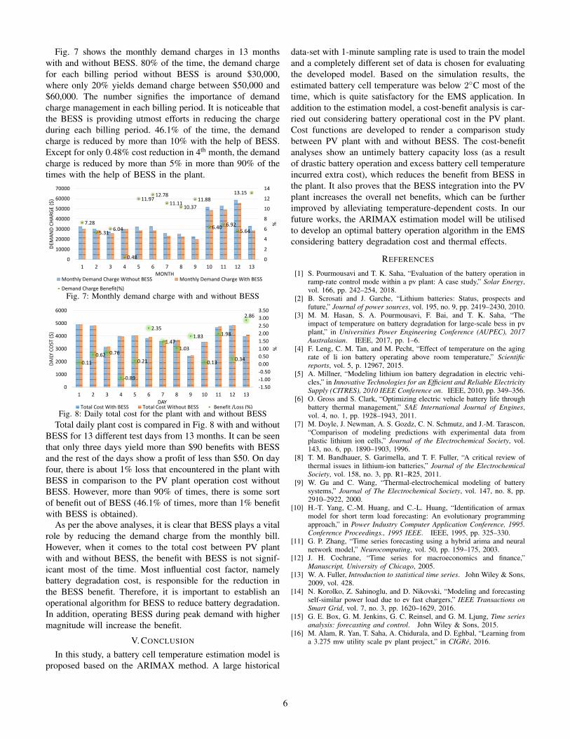
Fig. 7 shows the monthly demand charges in 13 monthswith and without BESS. 80% of the time, the demand chargefor each billing period without BESS is around $30,000,where only 20% yields demand charge between $50,000 and$60,000. The number signifies the importance of demandcharge management in each billing period. It is noticeable thatthe BESS is providing utmost efforts in reducing the chargeduring each billing period. 46.1% of the time, the demandcharge is reduced by more than 10% with the help of BESS.Except for only 0.48% cost reduction in 4th month, the demandcharge is reduced by more than 5% in more than 90% of thetimes with the help of BESS in the plant.

7.28

5.316.04

0.48

11.9712.78

11.1110.37

11.88

6.40 6.925.64

13.15

0

2

4

6

8

10

12

14

0

10000

20000

30000

40000

50000

60000

70000

1 2 3 4 5 6 7 8 9 10 11 12 13

%

DEM

AN

D C

HA

RG

E ($

)

MONTHMonthly Demand Charge Without BESS Monthly Demand Charge With BESS

Demand Charge Benefit(%)

Fig. 7: Monthly demand charge with and without BESS

0.11

0.62 0.76

-0.89

0.21

2.35

1.471.03

1.83

0.13

1.98

0.34

2.86

-1.50

-1.00

-0.50

0.00

0.50

1.00

1.50

2.00

2.50

3.00

3.50

0

1000

2000

3000

4000

5000

6000

1 2 3 4 5 6 7 8 9 10 11 12 13

%

DA

ILY

CO

ST (

$)

DAYTotal Cost With BESS Total Cost Without BESS Benefit /Loss (%)

Fig. 8: Daily total cost for the plant with and without BESSTotal daily plant cost is compared in Fig. 8 with and without

BESS for 13 different test days from 13 months. It can be seenthat only three days yield more than $90 benefits with BESSand the rest of the days show a profit of less than $50. On dayfour, there is about 1% loss that encountered in the plant withBESS in comparison to the PV plant operation cost withoutBESS. However, more than 90% of times, there is some sortof benefit out of BESS (46.1% of times, more than 1% benefitwith BESS is obtained).

As per the above analyses, it is clear that BESS plays a vitalrole by reducing the demand charge from the monthly bill.However, when it comes to the total cost between PV plantwith and without BESS, the benefit with BESS is not signif-icant most of the time. Most influential cost factor, namelybattery degradation cost, is responsible for the reduction inthe BESS benefit. Therefore, it is important to establish anoperational algorithm for BESS to reduce battery degradation.In addition, operating BESS during peak demand with highermagnitude will increase the benefit.

V. CONCLUSION

In this study, a battery cell temperature estimation model isproposed based on the ARIMAX method. A large historical

data-set with 1-minute sampling rate is used to train the modeland a completely different set of data is chosen for evaluatingthe developed model. Based on the simulation results, theestimated battery cell temperature was below 2◦C most of thetime, which is quite satisfactory for the EMS application. Inaddition to the estimation model, a cost-benefit analysis is car-ried out considering battery operational cost in the PV plant.Cost functions are developed to render a comparison studybetween PV plant with and without BESS. The cost-benefitanalyses show an untimely battery capacity loss (as a resultof drastic battery operation and excess battery cell temperatureincurred extra cost), which reduces the benefit from BESS inthe plant. It also proves that the BESS integration into the PVplant increases the overall net benefits, which can be furtherimproved by alleviating temperature-dependent costs. In ourfuture works, the ARIMAX estimation model will be utilisedto develop an optimal battery operation algorithm in the EMSconsidering battery degradation cost and thermal effects.

REFERENCES

[1] S. Pourmousavi and T. K. Saha, “Evaluation of the battery operation inramp-rate control mode within a pv plant: A case study,” Solar Energy,vol. 166, pp. 242–254, 2018.

[2] B. Scrosati and J. Garche, “Lithium batteries: Status, prospects andfuture,” Journal of power sources, vol. 195, no. 9, pp. 2419–2430, 2010.

[3] M. M. Hasan, S. A. Pourmousavi, F. Bai, and T. K. Saha, “Theimpact of temperature on battery degradation for large-scale bess in pvplant,” in Universities Power Engineering Conference (AUPEC), 2017Australasian. IEEE, 2017, pp. 1–6.

[4] F. Leng, C. M. Tan, and M. Pecht, “Effect of temperature on the agingrate of li ion battery operating above room temperature,” Scientificreports, vol. 5, p. 12967, 2015.

[5] A. Millner, “Modeling lithium ion battery degradation in electric vehi-cles,” in Innovative Technologies for an Efficient and Reliable ElectricitySupply (CITRES), 2010 IEEE Conference on. IEEE, 2010, pp. 349–356.

[6] O. Gross and S. Clark, “Optimizing electric vehicle battery life throughbattery thermal management,” SAE International Journal of Engines,vol. 4, no. 1, pp. 1928–1943, 2011.

[7] M. Doyle, J. Newman, A. S. Gozdz, C. N. Schmutz, and J.-M. Tarascon,“Comparison of modeling predictions with experimental data fromplastic lithium ion cells,” Journal of the Electrochemical Society, vol.143, no. 6, pp. 1890–1903, 1996.

[8] T. M. Bandhauer, S. Garimella, and T. F. Fuller, “A critical review ofthermal issues in lithium-ion batteries,” Journal of the ElectrochemicalSociety, vol. 158, no. 3, pp. R1–R25, 2011.

[9] W. Gu and C. Wang, “Thermal-electrochemical modeling of batterysystems,” Journal of The Electrochemical Society, vol. 147, no. 8, pp.2910–2922, 2000.

[10] H.-T. Yang, C.-M. Huang, and C.-L. Huang, “Identification of armaxmodel for short term load forecasting: An evolutionary programmingapproach,” in Power Industry Computer Application Conference, 1995.Conference Proceedings., 1995 IEEE. IEEE, 1995, pp. 325–330.

[11] G. P. Zhang, “Time series forecasting using a hybrid arima and neuralnetwork model,” Neurocomputing, vol. 50, pp. 159–175, 2003.

[12] J. H. Cochrane, “Time series for macroeconomics and finance,”Manuscript, University of Chicago, 2005.

[13] W. A. Fuller, Introduction to statistical time series. John Wiley & Sons,2009, vol. 428.

[14] N. Korolko, Z. Sahinoglu, and D. Nikovski, “Modeling and forecastingself-similar power load due to ev fast chargers,” IEEE Transactions onSmart Grid, vol. 7, no. 3, pp. 1620–1629, 2016.

[15] G. E. Box, G. M. Jenkins, G. C. Reinsel, and G. M. Ljung, Time seriesanalysis: forecasting and control. John Wiley & Sons, 2015.

[16] M. Alam, R. Yan, T. Saha, A. Chidurala, and D. Eghbal, “Learning froma 3.275 mw utility scale pv plant project,” in CIGRe, 2016.

6