Bayesian analysis of outlier problems using the Gibbs samplerbctill/papers/mocap/Verdinelli_Wasserman_1991.pdf · Statistics and Computing (1991) 1, 105-117 Bayesian analysis of outlier

Statistics and Computing (1991) 1, 105 -117

Bayesian analysis of outlier problems using the Gibbs sampler

I S A B E L L A V E R D I N E L L I 1'2 and L A R R Y W A S S E R M A N 2

1Department of Statistics, University of Rome, Piazzale A. Moro 5,00185 Rome, Italy 2Department of Statistics, Carnegie Mellon University, Pittsburgh, Pennsylvania 15213, USA

Received September 1990 and accepted November 1990

We consider the Bayesian analysis of outlier models. We show that the Gibbs sampler brings considerable conceptual and computational simplicity to the problem of calculating posterior marginals. Although other techniques for finding posterior marginals are available, the Gibbs sampling approach is notable for its ease of implementation. Allowing the probability of an outlier to he unknown introduces an extra parameter into the model but this turns out to involve only minor modification to the algorithm. We illustrate these ideas using a contaminated Gaussian distribution, a t-distribution, a contaminated binomial model and logistic regression.

Keywords: Contaminated normal, Gibbs sampling, Monte Carlo, outliers, posterior marginals

1. Introduction

Calculating posterior marginals for an outlier model typically involves difficult computations. The simplest example of this type of model is a finite mixture of normal distributions. Box and Tiao (1968), Guttman et al (1978), Abra- ham and Box (1978), Freeman (1980), Pettit and Smith (1984; 1985) and Titterington et al (1985) consider such models. All these authors comment on the computational problems in dealing with these models. For example, Freeman (1980), commenting on the work of Box and Tiao, Abraham and Box, Guttman et al, says that 'all three models can only be used with small sample sizes unless a maximum of two outliers is contemplated'.

We will show how for such models, Bayesian statistical analysis is simple using a Monte Carlo technique known as the Gibbs sampler (Geman and Geman, 1984; Tanner and Wong, 1987; Gelfand and Smith, 1990). Furthermore, we shall be able to carry out a fully Bayesian analysis. That is, we shall not assume that the number of outliers, or the probability that an observation is an outlier, is known. These simplifications are not needed when using the Gibbs algorithm.

An outlier is usually defined to be an observation that does not come from the assumed model or an extreme observation that is far away from the rest of the observations. Giving a precise definition to the concept of an

0960-3174/91 $03.00 + .12 �9 1991 Chapman & Hall

outlier is difficult since the notion of an 'extreme observation' is subtle. We shall not attempt a rigorous definition here. We refer the reader to Pettit and Smith (1985) for a discussion. An alternative view is presented in Chaloner and Brant (1988).

The simplest, and perhaps most studied, case is the normal model with mean # and variance o-:. To allow for the possibility of outliers, the model is enhanced so that the density for the observation Yi is of the form

f (Y i ]Iz, o-2, (., Ai ) =(1 - c)q~(y i I k t, 0 "2) +edp(y i ]# -}-Ai, 0 "2)

Here, ~b(y I/z, o-z) is the normal density with mean/z and variance a 2, and E ~ [0, 1] is the probability that the ith observation is from a normal model whose location is shifted by a factor Ai. This is known as the contaminated (location-shift) normal. Even if e is assumed known, this model is cumbersome since the analysis depends on the number of outliers in the model. Guttman et al (1978) assume that the number of outliers k is known and, further, that each subset of k observations is equally likely to be a set of outliers. Even so, the computations are still difficult.

Usually, the posterior marginal for # is the main con~ cern. Typically, we would also like to compute, for each observation, the posterior probability of that observation being an outlier. To be realistic, we should treat e as unknown as well. Doing so increases the dimension of the

106 Verdinelli and Wasserman

problem. Furthermore, the likelihood is difficult to work with since it is the product of mixtures. This makes finding posterior probabilities considerably more difficult. We shall see that the problem is well suited to the Gibbs sampler. Our main point is not that other techniques will not work, but that the Gibbs sampler brings striking conceptual simplicity to the computations. It is simplicity, not efficiency, that is the biggest obstacle to the implementation of Bayesian methods and this paper attempts to show how successful the Gibbs sampler is for obtaining such simplicity.

The reason why the Gibbs sampler brings such simplicity to outlier problems is that the Gibbs sampler operates by iterating two different stages of calculations. In the first stage, we assume we know which observations are outliers. This allows us to correct the outliers, and then we sample from the posterior using the corrected data. In the second stage, we assume that we know the true parameter values and, for each observation, we compute the posterior probability that the observation is an outlier. This is simple since the parameters are assumed to be known. Alternat- ing the two stages will eventually allow us to draw a sample from the posterior distribution. The details will be made clear in what follows. The important point is that the Gibbs sampler divides a difficult problem into a set of simpler problems.

The outline of this paper is as follows. Section 2 gives a brief description of the Gibbs sampler. In Section 3 we treat the contaminated normal location-scale problem. In Section 4, we consider using the student t-distribution as a model for the sampling distribution. This distribution has been suggested as an alternative to the contaminated normal as a way of modeling the fact that extreme observations are possible (Fraser, 1979; West, 1987; Lange et al, 1989).

Dealing with outliers in binomial problems (Winkler and Gaba, 1990) is also manageable, as we show in Section 5. We extend this to binomial regression (Pregibon, 1981; 1982; Copas, 1988) as well. Copas notes that, at most, a profile likelihood for each observation being an outlier is the best that can be obtained from the likelihood analysis. Here, we obtain the posterior probability that each observation is an outlier.

Section 6 contains a discussion of the results and indi- cates how the methods described in this paper can easily be generalized to handle regression problems and to handle outliers in other models such as exponential distributions (Pettit, 1988).

2. Gibbs sampling

In this section we give a short description of the Gibbs sampling algorithm, as considered in Gelfand and Smith (1990). What follows is the most basic form of the al-

gorithm, and we do not examine all possible variations. More details can be found in Gelfand and Smith (1990). The algorithm is intimately related to the notion of data augmentation and substitution sampling (Tanner and Wong, 1987).

We consider, for illustration, the case of three parameters only (01, 02, 03), and we assume that the three full conditional posterior distributions f l (011 02, 03, y), f2(02101,03, y) and f3(03101, 02, y) are available, meaning only that random samples can be drawn from them. Here, y denotes a vector (y~, Y2 . . . . . Yn) of n observations. I f f . is known in closed form and is a familiar distribution, then standard routines are available for drawing random numbers f r o m f . If fl , say, is not available in closed form, then one can obtain f l up to a proportionality constant by evaluating the product of the likelihood and the prior over a grid of values for 01, with 02, 03 and y fixed. Then, standard numerical techniques can be used to generate an observation from fl without renormalizing the product of the likelihood and prior. This is straightforward since 01 is one-dimensional. The simplest technique is probably the rejection sampling method (DeVroye, 1986). In its crudest form, one samples x uniformly on the support of f l (assuming the support is compact) and then samples w uniformly from 0 to m, where m is the maximum of k(O0. Here, k(O~) is the un-normalized product of the likelihood and prior (with 02, 03 and y fixed) so that f l = k/~ k. If w <- k(x) we keep x, otherwise we throw away x and draw a new x and a new w. We continue until we keep an x. The value that results is a random draw from f l . This can be a very inefficient way to generate random draws from f~ and many refinements are possible to make the process more efficient.

The Gibbs sampler is a simple way to generate observations from the joint posterior distribution so that the posterior marginal densities f(O~ l Y), f(o2 l Y) and f(03 l Y) can be estimated. To describe the algorithm, we begin by considering R groups of arbitrary starting values for the three parameters 0;, i = 1, 2, 3:

{(01) 1 (02)01 (03)1}, {(01) 2 (02) 2(03) 2} . . . . .

r . . . , {(01)0 (02)~) ( 3)0}, {(0l)g (02)g (03)0 R}

From each of these R groups of starting values we generate S sets of random numbers drawn from the conditional posterior distributions above. More specifically, consider the rth group-- the first set of random numbers, {(01)~, (02)~, (03) ] }, is obtained as follows:

(0~)~ is drawn from fl(O~](02)~, (03)~,y)

(02)] is drawn from f2(02[(0~)~1, (03)~, y)

(03)4 is drawn from f3(031(0~)~, (02)],y)

The second set of random numbers, {(01)~, (02)~, (03)~}, is

Bayesian analysis o f outlier problems using the Gibbs sampler 107

obtained as follows:

(0,)i is drawn from f~(01 [(02)~, (03)~, y)

(02)~ is drawn from f~(021 0 r , ( 1)2, (03)'1 Y) (03)~ is drawn f r o m f3(031(01)~, (02)-~ , y)

The procedure is repeated S times to generate the following collection of random numbers:

(01)~ (02)~ (03)~ (01)i (0~)i (0~)i

(01)~ (0~); (03);

(0~)~ (0s (03)~ The above step is repeated for r = 1 . . . . , R following R collections of S sets of random

(0,)I (0~)~ O3)I (01)~ (0~)~ (03)~

(01) ~ (0;)~ (03)~ i

(01)I (0s (0 )i

to obtain the numbers:

(01)~. (0~)~ (0!)~ r

(01) ft. (0;)~ (03)ffl'''"

(01)

(01)~ (0~)~ (03)~ (01)I (02)i (03)I

(01): (0;): (0;):

(01)~ (02)~ (03)~

(01)f (02)f (03)f[ (oi)~ (o~)f (o~)#

I It can be shown (Geman and Geman, 1984) that { (0 , ,02 ,03)~ , . . . , (01 ,02 ,03)~ , . . . , (01 ,02 ,03)~} is a sample of size R drawn from a c.d.f. Fs that converges, for large S, to the joint posterior distribution of (01, 02, 03) l Y" This sample will be used to estimate the posterior marginals. It may not be obvious to the reader that by drawing iteratively from conditionals we end up with a sample from the joint distribution. None the less, this is indeed what happens (see the aforementioned references for details).

The convergence of the algorithm is discussed in Gelfand and Smith (1990). Various techniques have been developed to check the convergence to the marginal distributions (see, for example, Zeger and Karim, 1991; Carlin et al, 1991). This remains an area of active research. Our experience suggests that R should be fairly large but that S need not be large. All the examples in this paper were done with S = 15. Typically, we found setting R to 200 or 400 to be sufficient. We judged this visually by repeating the entire process three times and then plotting the estimated marginals. For the last example of Section 5 we used R = 1000. Also, it is worth pointing out that the size of the resulting sample can be increased by including the

last j values {(0i)~_j+ 1, (Oi)"s /+2 . . . . , (0i)~}. This results in a final sample of size jR. Although the elements of the sample are not independent, the ergodic convergence of the process guarantees that we can still use this sample to estimate the posterior marginals. We did not use this technique in this paper.

Two methods can be used to estimate the posterior marginals from the samples. If the conditional posterior distributions are in closed form, then we estimate the density f(O 1 l Y), say, by f(O, I Y) where

1 R 0 r 0 r f(Ol ]y) --- ~r~=lfl(01 I( 2) s , ( 3 ) s , Y)

~Eoz,%ly(fj(O, [02, 03, Y))

= f ffl(OllO2,03,Y)f(O2,03lY)dO2dO~=f(OllY) If, instead, the conditional distributions are not specified in a closed form, f(011Y) is estimated from the sample

0 1 {( 1)s . . . . . (0l)~} using a kernel estimator (Tapia and Thompson, 1978). An alternative to the kernel estimator is to use the above formula by evaluating the product of the likelihood and prior over a grid of values of 0 l and normalizing this product by way of a one-dimensional integration. We are currently investigating this approach.

It is often the case that some of the parameters are conditionally independent. For example, it may turn out that f(O 1102, 03, y) does not depend on 02, say. This usually simplifies the procedure. Zeger and Karim (1989) discuss a simple graphical method for quickly identifying these instances of conditional independence.

3. The normal location-scale problem

We begin by considering the usual Gaussian location-scale problem. Let y = (Yl . . . . , y,) be a sample with density

f ( Yi [#, a2, E, Ai ) = (1 - E)dp( y i 112, 0"2) + (-q}( Yi It 2 + Ai, 0"2)

It is convenient to re-express the model as follows. Let 6 = (61 . . . . ,6 , ) be independent Bernoulli trials with success probability E, and let A = ( A 1 , . . . , A,). Then,

Yi l #, a2, A, 6 ,-~ N(12 + 6eA~, ~2)

Note that each Yi is conditionally independent of e. First, consider the case where E is known. We use the standard conjugate priors for p and 0"2. That is, we assume that 12 ~ N(O, v 2) and that 0"2 has an inverted )~2 distribution with parameters v and 2. We also consider the A,.s to be independent, each with a N(0, z z) prior distribution.

T o employ the Gibbs sampler we choose R arbitrary starting values for the 2 + 2 n parameters 12~,a~, (0i)~, (A;)~, (i = 1 . . . . , n; r = 1, . . . , R). To generate the random numbers, we need the densities f1(12 ] y , a 2, 6, A, E),

108 Verd ine l l i a n d W a s s e r m a n

fz(c~2ly, g ,&A,c ) , f3(~ly,#,0.2, A, 0 and f 4 ( A l y , ~ , o 2, ~, e) where it is understood that f3 is a probability mass function. We now derive these conditional distributions.

First, note that conditional on the data and the other parameters, both # and 0.2 are independent of E. In order to obtain the distribution of # [0.z ~, A, y we consider y* = (y* . . . . , y*) where y * = y ~ - fi~A~. Thus, y* is iden- tical to the original data except that the outliers have been corrected by subtracting off the location shift A~. This correction is possible since both A and ~ are known at this step. Now, the y* s are independent samples from a N(#, 0.2) distribution, with 0.2 known. Thus, the formula for updating a conjugate prior (DeGroot, 1970) can be used and we have that # [y, 0.z ,& A is N(a, b) where a = { O / v 2 + n ~ * / 0 . 2 } { 1 / v 2 + n / 0 . z } -~, b - l = 1 / v 2 + n / 0 . 2,

and )7" is the average of the y* s. Standard routines can be used to generate the random draw of/~.

A similar argument is used for fz. We find y* and then employ the update formula for 0 .2 with # known. Thus, 0.2]y, #, ~, A has an inverted Z 2 distribution. Specifically, ( n s 2 + v2)/0. 2 has a )~2 distribution with n + v degrees of freedom, where s 2 = E ( y * - #)2/n.

Now consider f3. It is easy to see that, conditional on the data and the other parameters, each 6i is an independent Bernoulli trial with success probability

(o(( y~ - # - A~) /0.)e

P' = (o((y~ - # - A~) /0.)E + (o((y i -- #)/0.)(1 -- E)

where ~b(.) -= ~b(-[0, 1) is the density function for a standard normal distribution.

Finally consider f4. The Ags are conditionally independent given #, 0., e, ~, y. We derive the conditional distribution for Ai. If 6 ;= 1, then y~-~t is a sample from a N(A~,0. 2) distribution. Again, the standard conjugate update shows that Ag I Y, #, 0.2, 6~ = 1, E has a N(c, d)

distribution where

(y, - #)/0.~ C =

1/z 2 + 1/0. 2

d - 1 = 1/~ 2 + 1/0. 2

If, instead, 6i = 0, then we have no information on Az (that is, the likelihood for A~ is fiat) so that the conditional distribution A~ty, #, a z, 6~ = O, e is simply its prior distribution, namely, N(0, "c:). If one wanted to use an im- proper prior for A , this could be approximated in the algorithm by using a large value for z.

The Gibbs sampler can now be easily implemented. Standard routines can be used to generate random numbers from the required distributions. The procedure is repeated S times, resulting at the Sth step in samples

u i , . . . , . g

(0.2) 1 (0.2) g S , ' ' ' '

( 3 , ) ~ , . . . , ( 6 ; ) ~ , f o r i = l . . . . . n

( A ; ) ~ , . . . , ( A , ) s R, f o r i = l . . . . . n

The posterior marginal for/~ may be estimated as

1 R

f(~ ly) -- ~ , 0(# I a- br)

where

oIv 2 + ny* l (a2 )9 a, = 1/v2 + n/(0.2)r ~

b 7 ~ = 1/v 2 + n/(0.2)~s

y . = y , - O,)~s (Ai)~s

Similarly, the posterior probability that Yi is an outlier is estimated by

1 n e ~ b ( ( y * - # ~ - ( A i ) ~ ) / ( a ) ~ )

3r 2 = ~ ed~((y* - #~s - (AYs)/(a)~s) + (1 - c)4((y* - g~)/(a)~)

The posterior for a is of less interest and we do not bother to estimate it.

As an example, we used the infamous Darwin data (Fisher, 1960). The data consist of 15 height differences of cross- and self-fertilized plants. The two smallest observations ( - 6 7 and -48 ) are usually regarded as possible outliers. We used E = 0.05 and v = z = 1000. This value of e is typically regarded as being reasonable for these data (Box and Tiao, 1968). The large values of v and z are used to reproduce the usual fiat priors used in this problem. Similarly, we take v - - 0 to produce the non-informative prior for a. But note that using informative priors does not make the calculations any more difficult. We used R = 200 and S = 15. For the purposes of illustration, we repeated our entire analysis three times to expose the variability of the procedure.

The estimated posteriors for # and a are plotted in Figs l a and lb. When feasible, the plots include the three estimated posteriors corresponding to the three repeated runs. In some cases, such as Fig. lb, it is difficult to distinguish the different runs by eye, so the results of only one run are displayed. An informal graphical inspection of the three densities in the plot suggests that the process has converged. Larger values of R can be used to reduce the variability even further. If the possibility of outliers is excluded by setting E = 0, the posterior for # will have a mode at 20.933 (Box and Tiao, 1968). Allowing for out- tiers causes the posterior to be shifted to the right so that the effect of the two extreme observations has been down- weighted (for similar analyses, see Box and Tiao, 1968; Abraham and Box, 1978). The two smallest observations are regarded as outliers in this data set and indeed, we see that the smallest observation (y = - 6 7 ) has a posterior probability of almost 0.40 of being an outlier, while the second smallest observation (y = - 4 8 ) has a posterior probability of slightly over 0.20 of being an outlier. The

B a y e s i a n ana lys i s o f out l ier p r o b l e m s us ing the Gibbs s a m p l e r 109

~o ( :3

o

i t

/ /

/

r

I I I I f I I

0 10 20 30 40 50 60

POSTERIOR MARGINAL FOR ,u

Fig. la. Posterior marginals for It based on a contaminated Nor- mal model with E = O.05 for the Darwin data, Each o f the three curves corresponds to a complete run o f the Gibbs sampler.

remainder of the observations have relatively small posterior probabilities of being outliers, with the largest being the last observation (y = 75), with probability 0.075. Note that the posterior probability that a subset of observations are outliers can be estimated by counting the proportion of the corresponding fit s that were ls on the sample from the Gibbs algorithm. In particular, to estimate the probability that there are no outliers, we need only count the proportion of times that all 6is were 0s. This turned out to be 0.435. Also, the probability that there were one, two, three or four outliers is 0335, 0.180, 0.035 and 0.015, respectively. The program to carry out these calculations is very simple and was implemented in New S (Becker et al, 1988).

We now consider the case where ~ is unknown. To our knowledge, this case has not been treated before. We are thus adding another parameter to the model. Using the Gibbs sampler, this turns out to be extremely simple as well. The densities f l , f2, f3 and f4 remain unchanged since they are conditional on E. But we need a fifth conditional posterior, namely, the distribution for e conditional on the data and the rest of the parameters. We take ~ to have a

c O

r cl -

o rr rr ~ 7 r I I -

I I I I I I I

-60 -40 -20 0 20 40 60 80

b POSTERIOR PROBABILITY THAT EACH OBSERVATION IS AN OUTLIER

Fig, lb. Posterior marginal probability that each observation is an outlier based on a contaminated Normal model with ~ = O.05 for the Darwin data.

beta(p1, P2) prior distribution. A flat prior is not appropriate, for, presumably, we would not be conducting the experiment if there were an exceedingly large probability of many outliers. As mentioned before, several authors have considered a value of 0.05 to be reasonable for E (Box and Tiao, 1968). We thus take the mean of the prior for E to be 0.05. It seems reasonable to asst~me that an observation has less than half a chance of being an outlier with high probability. If we assume that P(E < 0.5) = 0.99, then this implies that pl = 0.1842 and P2 = 3.5. Now, since we are conditioning on 6, this posterior is straightforward. It is readily seen that the conditional distribution for e depends only on 6. Let k be the number of 6;s that are equal to one. Then we simply have a binomial experiment with k successes and a beta prior. Hence the required density is beta(p~ + k, P2 + n - k). Again, we can generate random numbers from this distribution using standard routines. The posterior marginal for E is estimated by

1 R f(~ [y) = ~ ~. B(p~ + k(r), P2 + n - k(r))


,:5

o

o d

..... f~S �9

i p i

0 10 20 30 40 50 60

POSTERIOR MARGINAL FOR/t

Q

CO

r

O i

0.0 0.2

l

0.4 0.6 0.8 1.0

a POSTERIOR MARGINAL FOR s

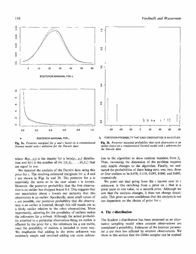
Fig. 2a. Posterior marginal for I ~ and E based on a contaminated Normal model with c unknown for the Darwin data.

o

0o ,:5

o

<5

o d

b rT ~ r T TT I I I I I t I

-60 -40 -20 0 20 40 60 80


Fig. 2b. Posterior marginal probability that each observation is an outlier based on a contaminated Normal model with E unknown for the Darwin data.

where B(pl, P2) is the density for a beta(p1, P2) distribution and k(r) is the number of the {( 1)s , - . (6,)~} that are equal to one.

We repeated the analysis of the Darwin data using this prior for ~. The resulting estimated marginals for #, 6 and c are shown in Figs 2a and 2b. The posterior for /~ is essentially the same as in the case where e is known. However, the posterior probability that the first observation is an outlier has dropped below 0.4. This suggests that our uncertainty about e lowers our certainty that this observation is an outlier. Specifically, since small values of E are possible, our posterior probability that the observation is an outlier is lowered, though this still stands out as a likely outlier relative to the other observations. More importantly, allowing for the possibility of outliers makes the inferences for # robust. Although the actual probability attached to a particular observation being an outlier is affected by the prior for e, the inferences for # are stable, once the possibility of outliers is included in some way. We emphasize that adding in the extra unknown was extremely simple and involved adding one extra subrou-

tine to the algorithm to draw random numbers from fs- Thus, increasing the dimension of the problem requires only simple changes to the algorithm. Finally, we estimated the probabilities of there being zero, one, two, three or four outliers to be 0.670, 0.110, 0.095, 0.060, and 0.045, respectively.

We point out that going from the c known case to c unknown, is like switching from a prior on E that is a point mass at one value, to a smooth prior. Although we saw that the analysis changes, it does not change drasti- cally. This gives us some confidence that the analysis is not too dependent on the choice of prior for E.

4. The t-distribution

The Student t-distribution has been proposed as an alternative sampling model when extreme observations are considered a possibility. Estimates of the location parameter # are then less affected by extreme observations. We show in this section that the Gibbs sampler can be applied

Bayesian analysis of outlier problems using the Gibbs sampler 111

for finding the marginal posterior for # in this case. Thus, we assume that the density for Yi is

~ + 1

f(Yi I#, a2, ~) oc " + a 2

It is convenient to introduce, for each observation, an extra parameter We such that

Y i I # , 0"2 ' ;Vi ~ N(#, a2W~ -x)

and to assume that the W,.s are independently distributed as gamma random variables with parameters (a/2, a/2). It is straightforward to see that the marginal distribution for each observation

[#, a 2, ~z) = f f (y , ]#, aT-, Wi)f(W z f (y , I a) dW,

is then a t-distribution with a degrees of freedom. In this way, we have simply rewritten the t-distribution as a mixture of normals introducing n extra parameters W,.. Note that each Ye is conditionally independent of a given Wi. Distributions other than the Student t can be expressed as a mixture of normals (see, for example, West, 1987). Hence, it is trivial to adapt the methods in this section to deal with any scale mixture of normals simply by replacing the gamma distribution with the required mixing distribution. The Gibbs sampler can thus be used to develop a complete Bayesian analysis for a large class of models.

The set of parameters that we are going to consider here is {p, 0.2, W, a} where W = (Wi, W7-, . . . , IV,). Let us assume, at first, that ~ is known and let the prior distributions for # and 0"7- be, as in Section 3, normal and inverted chi-squared. Values for e in the range of 1 to 7 have been cited as being reasonable (see Fraser, 1979, p. 37; Lange et al, 1989). For now, we shall take e = 3. The conditional posterior distributions required to implement the Gibbs algorithm can be readily derived. That is, it can be seen through successive application of the conjugate update formulas, together with the fact that Yi ]#, 0.7-, W; has a N(p, o -2 W,7 l) distribution, that # [0 -2, W, y,-~N(a, b), where

O/vT- + (:~ yi w,)#rT- a =

U--7- § ( ~ W i ) o . --2

1 Y~W,. b - ~ = ~ + a2

Further, we obtain that o-21/~, W, y has an inverted chi- squared distribution. More precisely:

Z IV/(yi -- #) 2 + v2 2

0.2 X n + v

Also, we have the W/.s are conditionally independent and W~t:t , o-7-,y is a gamma distribution with parameters (a + 1)/2 and [(y~ - #)2/0.7- + ~]/2.

g <5

oJ ,q o

,5

o o

/

I I I I I

0 10 20 30 40

I I 50 60

POSTERIOR MARGINAL FOR ,u

Fig. 3. Posterior marginal for # based on a t distribution with three degrees of freedom for the Darwin data.

Therefore, all the required conditional posterior distributions are available analytically and, as described in Section 2, we proceed generating random numbers from these distributions using standard routines. After S iterations of the algorithm we obtain samples of size R for the n + 2 parameters considered.

In particular, the marginal posterior density for ~t for the Darwin data, shown in Fig. 3, has been estimated from the samples (0.2)~, . . . , ( a 2 ) } , . . . , (a2)g and (Wi) ~ . . . . , ( W , ) s . . . . . W R r ( i )s , for i = 1,2 . . . . , n b y

1 R 1 R f (# lY) =-'~r~lf(# ](O'2)s, (W)~, y) = ~ Z ~b(p lar, br)

-- r = l

where

O/v 2 + ( z y,(Wi)D/(~7-)r~ a r - - V - -2 _[_ ( ~ r - -2 r (W,-) s)(~ ),

b ; 1 = ~ + Y, (Wi)~ (GT-)}

We found that the estimates based on R -- 200 were not as

112 Verdine l l i a n d W a s s e r m a n

stable as in the contaminated normal case. The estimates in Fig. 3 are based on R --400.

So far, the shape parameter a has been considered as known. It is far more realistic to assume that a is unknown. We now proceed with a regarded as an unknown parameter.

As e varies from 1 to oe the class of t-distributions varies from the Cauchy to the normal. It is convenient to define /3 = 1/e and we use a beta distribution for/3 with parameters 1.75 and 2.5. In this way, the mode of/3 is 1/3. Also we have that P{1/3 </3 < 1/2} = 0.26, P{/3 > 1/3} = 0.6, P{f i < 1/10} = 0.06. We tried to choose a prior that reflected a fair amount of uncertainty about/3, that had a mode at a reasonable value (/3 = 1/3) and not too much probability near normality. We do not claim that this is an optimum prior in any sense. An interesting topic for luther research is to determine reasonable prior distributions for parameters that index outlier models. One referee suggested putting a point mass on the normal model (/3 = 0). This would especially be appropriate if one were interested in computing a Bayes factor for the hypothesis that the

normal model is correct. However, since our goal is to protect us from outliers by allowing for the possibility of extreme observations, rather than model identification, we feel that the prior we have chosen is sufficient.

This is a case in which the conditional posterior distribution of/3 is not in closed form. In fact, a prior for/3, or a, cannot be expressed within a conjugate family; hence we only have the kernel of the distribution:

f(/3 l W, ~, a, y) =f(/3 [VO ocf(/3) f i f ( W i 1/3) i = l

OC ~ ~ - ( 1 / - / 2 ~ n i = l fi W/~ exp - - ~ i=1 ~ ~Vi

Here, f(/3) is the prior density for /3. Note that we are dealing here with the distribution of/3 conditional on W, since the introduction of the new variables Wi s makes the model for the data independent of the shape parameter 1//3. In other words, /3 is only influenced by W and the effect of the data on/3 is through W.

Random numbers can be drawn from f(/3 Iw) using the rejection method (Section 2). Then the marginal posterior

o

E ,5

o c5

\

/ / i

/

I I I t L I

0 10 20 30 40 50 60

a POSTERIOR MARGINAL FOR #

Fig. 4a. Posterior marginal for # based on a t distribution with degrees o f freedom ct unknown for the Darwin data.

ot O

O _

d

~3

O

f,

I

I / /

I 2 c5

!

I I I I t I I L

-6 -4 -2 0 2 4 6

b POSTERIOR MARGINAL FOR ALPHA IN LOGIT SCALE:

Fig. 4b. Posterior marginal for logit([1) based on a t distribution with degrees of freedom ot unknown for the Darwin data where a = 1/[1.


distribution can be estimated from the sample by a kernel density estimator. The marginal for # is plotted in Fig. 4a using R = 400. We see that the marginal for # is not greatly affected by our uncertainty about/?. We have also obtained the posterior for/~ using a kernel density estimator; see Fig. 4b. As expected, this posterior is very similar to the prior since it requires a large amount of data to learn about tail thickness. The reason for including/? as an unknown parameter is not to learn about/~, but rather to lead to a more honest analysis for p.

It is interesting to consider a different parameterization for the shape parameter. Let 7 = log(/~/(1-/~)) be the logit of /L When 7 ~ - oc the sampling distribution is normal and when ~---, + oo the sampling distribution is Cauchy. The origin corresponds to e = 2. This suggests that values usually employed, namely around e = 2 and c~ = 3 are, in some sense, mid-way between the normal and the Cauchy distributions.

5. B inomia l mode l s

Winkler and Gaba (1990) considered the following problem. We sample w = ( w ~ , . . . , w~) where each wi is an independent Bernoulli trial with success probability p. Then, each wi is either switched or not switched, where the switching takes place with probability E. That is, we ob- serve y~ where, conditional on w~, y~=(1-cS~)w~+ 6 i (1 -w~) and each 6e is a Bernoulli trial with success probability e. We let 6 = (6~ . . . . . 6,). This may be viewed as a binomial version of the outlier problem. In this case, an outlier is simply a Bernoulli observation that has been switched. The posterior marginals for p and E are derived in Winkler and Gaba (1990). As in the Gaussian case, the computations are not simple. We point out that p and e are not identifiable in this model. We will be using proper priors, however, so that the posterior marginals are well defined. In this situation, the prior information is quite important.

To use the Gibbs sampler, we need f ( p [ E , y , 6), f(EIp, y, 6) and f(6~lp, E, y). Following Winkler and Gaba (1990) we use a beta(s,/~) prior f o rp and a beta(a, b) prior for e. We now derive the three required conditional posterior distributions.

Consider p[e, y, 6. Since 6 is given, we can define the corrected data vector w = (w~ . . . . , w~) where w e = ( 1 - 6 ~ ) y e + f ~ ( 1 - y z ) . Then, w is a vector of Bernoulli observations so that the required conditional posterior is beta(e + Z we,/~ + n - Z wi). Similarly, E ]p, y, 6 has a beta(a + Z 6i, b + n - lg 6~) distribution. Finally, it is easy to see that fig [p, e, y is Bernoulli with success probability q~ where

ep ~t( 1 -- p) 1 ,'i q~ - epW~(1 _p)~-w~ + (1 -- e)pY~(1 --p)~ Y~

It is straightforward to generate the required random numbers. After S iterations, this leads to samples

pL...

6 i . , f i r ( i ) s , . . ( i)s, i = l , . . . , n

The estimates of the posterior marginals are thus

f ( P lY) = -k r21= n e -J[- ~i (wi)rs' ~ "~ Fl -- ~i (wi)rs '

f(EIy)= B a+ r ~ I " '

and

1 R -P(cSi -- I I Y) -- ~ r~1

e(p}) (w~)~(l __p~)l -- (w i)r S

E(p~) (w,)~(l -p~)~-('~,)~ § I - E)(p~)y,(I -p"s) ~ --Yl

We applied this to a data set involving self reported delinquent behaviour (Gould, 1969) as analysed by Win- kler and Gaba. Of 104 college students who were asked if they had beaten someone up, 21 said they had. Here, Yi = 1 corresponds to an affirmative response. Based on information from Clark and Tifft (1966), Winkler and Gaba proposed a beta(2, 8) distribution for p and a beta(2, 18) distribution for r The resulting posteriors for p and E, based on R- -400 , are shown in Fig. 5. The posteriors are the same as those displayed in Winkler and Gaba (1990). The probability that Ye is an outlier is 0.35 if y ; - -1 and is 0.01 if y ; - -0 . It could be agreed that the outlier model should be expanded to allow a probability q of a 1 being switched to a 0 and a probability r of a 0 being switched to a 1. It is obvious how to generalize the Gibbs sampler to deal with this case; the calculations are not any more difficult. We shall not pursue these details here.

We now consider the more interesting case where a regressor x is available. Specifically, suppose that each w; is Bernoulli with success probability

exp(e § ~Xi) p~ (~,/~) =

1 + exp(e +/~x;)

where e and/~ are unknown regression parameters and x~ is the observed value of some predictor variable x. This is the standard logistic regression model (McCullagh and Nelder, 1989, p. 108).

The problem of outliers in logistic regression is dealt with in Pregibon (1981; 1982) and Copas (1988). In his discussion of Copas, O'Hagan (1988) suggests that a Bayesian approach is possible, though he acknowledges the heavy computational burden that this entails. And Davison (1988), discussing the same paper, shows that Laplace's method of approximating integrals can be used to approximate the predictive probability of an observa-


tNi

A Z

ft f/

i

0.0 0.1 0.2

~J c5

POSTERIOR MARGINAL FOR p

o

o ,5

o. o

0.3 0.4 0

i i

5 10 15 20 25 30

MARGINAL POSTERIOR FOR a

0

\

\

i i

0.0 0.1 0.2 0.3 0.4

a POSTERIOR MARGINAL FOR E

F i g . 5 . P o s t e r i o r m a r g i n a l s f o r p a n d e f o r the B i n o m i a l m o d e l .

o

i i i

-1.0 -0.5 0.0 0.5

MARGINAL POSTERIOR FOR b

tion given the rest of the data and thus he obtains a Bayesian method for identifying suspicious observations. Here, as in the previous cases, we consider a completely Bayesian approach. As before, we assume that there is a probability e that w i is switched to 1 - w~. More formally, we assume that y~ = (1 - ~ i ) w i ~- (~i (1 - w i ) where S~ is Bernoulli with success probability E. This is the model used by Copas (1988). Ekholm and Palmgren (1982) and Palm- gren and Ekholm (1987) propose more general models for contaminated binary data. We shall not pursue those models here, though it should be possible to extend our methods to deal with those models.

The likelihood function based on the uncontaminated data w is

L.(~ , /~ , E) = I-I p,(~, fl)w'( 1 - p i ( ce, fl))l-w, i

Convenient conjugate priors do not exist for this model. This does not present a serious problem for our analysis. To sample from the col lition~l "~" utions we resort to

the rejection method described in Section 2. We now describe the process in more detail. We took E to be a priori independent of c~ and/~ with a B(a, b) distribution. We let

and/~ have an arbitrary prior density denoted by rc(~,/3). First we consider f ( ~ I fl, E, 3, y, x). Let w; = (1 - 6t)yi+

6i (1 - y i ) . The posterior conditional for ~ is proportional to L,,(~, fl, e)n(~, fl, E) where fl and e are fixed. We draw a random ~ from this distribution using the rejection method described in Section 2. The method for drawing fl is the same.

We can find f(E [ ~,/~, 3, y, x) in closed form. First note that E is conditionally independent of ~, /~, y and x. Let k = Z 6g. Then obviously, the conditional distribution for E is B(a +k , b + n - k ) .

Finally, consider ~ [~,//, E, y, x. Each 6i is Bernoulli with success probability

Ep] - y i ( l - p i ) y'

Ep~-Y'(1 -p,)Y' + (1 - QpY'(I _ p ; ) l - y ,

where Pi --Pi (~,/~).


i'M

d

g d

0

0 d

/ ; / /

0 5 10 15 20 25 30 0.0

MARGINAL~POSTERIOR FOR

0.2 0.4 0.6 0.8 1.0

MARGINAL POSTERIOR FOR E

0 ,::5

i i r

-1.0 -0.5 0.0 0.5

a MARGINAL POSTERIOR FOR /~

Fig. 6a. Posterior marginals for ~ and fl for the Challenger data.

C~ .c

CO c5

~O c5

c5

CM

c5

O c5

T I , , . . . .

i r

55 60 65 70 75 80


Fig. 6b. Posterior marginals for E and posterior marginal probabi- ity that each observation is an outlier.]'or the Challenger data.

We illustrate the method with data from Dalai et al (1989). They analysed data on 23 launches of the space shuttle to estimate the probability of an O-ring failure on the day the space shuttle Challenger was launched. The data we used was a binary outcome, indicating an incident with the O-rings (erosion or blowby) and the regressor was joint temperature. Following Dalai et al, we used a logistic model but we allowed for outliers. We used uniform priors for a and/Y and a beta(0.1842, 3.5) prior for c as in Section 3. Posterior marginals were estimated from the samples by kernel density estimation, as suggested in Gelfand and Smith (1990). Because we relied on kernel density estimators, we increased R to 1000 but kept S = 15. We used FORTRAN since S was too slow in this case.

The estimated posteriors are in Figs. 6a and 6b. The O-ring failure at 75~ is an outlier with probability 0.22. This is consistent with the Dalai et al analysis. Similarly, the failures at 70~ each have probability 0.14 of being outliers. The failure of 63~ has probability 0.05 of being an outlier. While this is not very large, it is interesting to

note that the Dalai et al analysis does not seem to flag the observations at 63~ at all. This may be a masking effect. As O'Hagan (1988) remarks, masking is not a problem in the Bayesian approach since we are computing the marginal probability that each observation is an outlier. This averages over the possibilities that there are simulta- neously other outliers.

6. Discussion

Our emphasis has been on demonstrating the simplicity of the Gibbs sampling approach to the computation of posterior marginals in outlier problems. Other approaches may well provide faster, more efficient routines for doing the same task, but what the Gibbs approach has to offer is greater flexibility and less programming effort. That is, less computer efficiency is traded for more human efficiency.

The conceptual simplicity of the approach makes it easy to write the necessary programs and, having written the programs, it is easy to change them to handle new


problems. For example, to go from ~ known to e unknown in the e contamination model, we needed only add one new subroutine, namely a routine to draw from the conditional distribution for c. In S, this involved adding one new function of four lines of code. Similarly, to replace the t-distribution with a different mixture of normals would involve replacing the gamma function with the appropriate mixing distribution. Thus, one small part of the program would be modified: instead of drawing random gammas we would draw from a different distribution.

The methods in Section 3 and 4 can easily be extended to the regression case. Instead of drawing p from a normal distribution, for example, we would draw fl from a multi- variable normal distribution, where • = ( i l l , . . . , tip) are the regression parameters. Similarly, the other conditional distributions would be adapted in the obvious way. In the case of logistic regression, sampling from the posterior conditionals of the regressors i l l , . . - , tip would best be done one at a time. But the sampling method would be exactly the same as that used in Section 5 so we would essentially just repeat that part of the program p times. The point is that increasing the dimension of the problem increases the execution time of the program but it does not increase the complexity of the program. There is no need to deal with high-dimensional grids, for example. In a sense, the Gibbs sampler replaces a difficult high-dimensional problem with a series of simple one-dimensional problems.

It is easy to adapt the Gibbs sampler to deal with outliers for other sampling models. For example, Pettit (1988) considers sampling from an exponential when outliers are possible. He derives an insightful approximation to find the Bayes factor for a particular observation being an outlier. Using the Gibbs sampler for this problem is essentially the same as the contaminated normal case in Section 3. In particular, at most steps in the algorithm, we are conditioning on the vector ~ = (61, . . . , fin) that tells us which observations are outliers so that the outliers can be corrected and the usual Bayesian conjugate distributions can be used. And the distribution of 6 given the other parameters is straightforward. Thus, a fully Bayesian analysis is possible and the posterior probability that a particular observation is an outlier can be estimated, as can the posterior probability that a set of observations is an outlier.

Acknowledgments

We are grateful to Rob Kass for suggesting that we apply these methods to the t-distribution and for many other useful discussions. We also thank Brad Carlin, Nick Pol- son, Joel Greenhouse and two referees for helpful com- ments. This work was completed while the first author was visiting the Department of Statistics at Carnegie Mellon

University and was partially supported by the Italian Research Council (CNR). The second author was supported by the Natural Sciences and Engineering Research Council of Canada.

References

Abraham, B. and Box, G. E. P. (1978) Linear models and spurious observations. Applied Statistics, 27, 13!-138.

Becker, R. A., Chambers, J. M. and Wilks, A. R. (1988) The New S Language, Wadsworth, Pacific Grove, California.

Box, G. E. P. and Tiao, G. C. (1968) A Bayesian approach to some outlier problems. Biometrika, 55, 119-129.

Carlin, B., Gelfand, A. E. and Smith, A. F. M. (1989) Hier- archical Bayes analysis of change point problems. To appear in Applied Statistics.

Chaloner, K. and Brant, R. (1988) A Bayesian approach to outlier detection and residual analysis. Biometrika, 75, 651- 660.

Clark, J. P. and Tifft, L. L. (1966) Polygraph and interview validation of s~lf reported deviant behavior. American Soci- ological Review, 31, 516-523.

Copas, J. B. (1988) Binary regression models for contaminated models. Journal of the Royal Statistical Society Series B, 50, 225 -265.

Dalai, S. R., Fowlkes, E. B. and Hoadley, B. (1969) Risk analysis of the space shuttle: pre-Challenger prediction of failure. Journal of the American Statistical Association, 84, 945 -957.

Davison, A. C. (1988) Discussion on Copas. Journal of the Royal Statistical Society Series B, 50, 258-259.

DeGroot, M. H. (1970) Optimal Statistical Decisions. McGraw- Hill, New York.

DeVroye, L. (1986) Non-uniform Random Variate Generation. Springer-Verlag, New York.

Ekholm, A. and Palmgren, J. (1982) A model for a binary response with misclassification. GLIM-82: Proceedings of the International Conference on Generalized Linear Models, R. Gilchrist (Ed), Springer-Verlag, Heidelberg, pp. 128-43.

Fisher, R. A. (1960) The Design of Experiments (7th edn), Oliver and Boyd, Edinburgh.

Fraser, D. A. S. (1979) Inference and Linear Models, McGraw- Hill, New York.

Freeman, P. R. (1980) On the number of outliers in data from a linear model, in Bayesian Statistics, Proceedings of the First International Meeting held in Valencia (Spain), J. M. Bernardo, M. H. DeGroot, D. V. Lindley and A. F. M. Smith (eds), 347-382.

Gelfand, A. E. and Smith, A. F. M. (1990) Sampling based approaches to calculating marginal densities. Journal of the American Statistical Association.

German, S. and Geman, D. (1984) Stochastic relaxation, Gibbs distributions and the Bayesian restoration of images. IEEE Transactions on Pattern Analysis and Machine Intelligence, 6, 721-741.

Gould, L. L. (1969) Who defines delinquency: A comparison of self-reported and officially reported indices of delinquency for three racial groups. Social Problems, 16, 325-336.


Guttman, I., Dutter, R. and Freeman, P. (1978) Care and handling of univariate outliers in the general linear model to detect spuriosity--a Bayesian approach. Technometrics, 20, 187- 194.

Lange, K. L., Little, R. J. A. an d Taylor, J. M. G. (1989) Robust statistical modeling using the t distribution. Journal of the American Statistical Association, 84, 881-896.

McCullagh, P. and Nelder, J. A. (1989) Generalized Linear Models (2nd edn), Chapman and Hall, London.

O'Hagan, A. (1988) Discussion on Copas. Journal of the Royal Statistical Society Series B, 50, 259.

Palmgren, J. and Ekholm, A. (1987) Exponential family nonlinear models for categorical data with error of observation. Appl. Stochast. Model Data Anal., 3, 111-124.

Pettit, L. I. (1988) Bayes methods for outliers in exponential samples. Journal of the Royal Statistical Society Series B, 50, 371-380.

Pettit, L. I. and Smith, A. F. M. (1984) Bulletin of the International Statistical Institute: Proceedings of the 44th session, 292-306.

Pettit, L. I. and Smith, A. F. M. (1985) Outliers and influential observations in linear models, in Bayesian Statistics 2, J. M. Bernardo, M. H. DeGroot, D. V. Lindley and A. F. M. Smith (eds), North-Holland, Amsterdam, pp. 473-494.

Pregibon, D. (1981) Logistic regression diagnostics. Ann. Statist. 9, 705-724.

Pregibon, D. (1982) Resistant fits for some commonly used logistic models with medical applications. Biometrics, 38, 485 -498.

Tanner, M. and Wong, W. (1987) The calculation of posterior distributions by data augmentation (with discussion). Journal of the American Statistical Association, 82, 528- 550.

Tapia, R. A. and Thompson, J. R. (1978) Nonparametric Proba- bility Density Estimation, Johns Hopkins University Press, Baltimore, Maryland.

Yitterington, D. M., Smith, A. F. M. and Makov, U. E. (1985) Statistical Analysis of Finite Mixture Distributions, Wiley, New York.

West, M. (1984) Outlier models and prior distributions in Bayesian linear regression. J. R. Statist. B., 46, 431-439.

West, M. (1987) On scale mixtures of normal distributions. Biometrika, 74, 646-648.

Winkler, R. L. and Gaba, A. (1990) Inference with imperfect sampling from a Bernoulli process, in Bayesian and Likeli- hood Methods in Statistics and Econometrics, S. Geisser, J. S. Hodges, S. J. Press and A. Zellner (eds), North-Holland, Amsterdam.

Zeger, S. L. and Karim, M. R. (1991) Generalized linear models with random effects: a Gibbs sampling approach. Journal of the American Statistical Association, 86, 79-86.

Documents

Bayesian analysis of outlier problems using the Gibbs samplerbctill/papers/mocap/Verdinelli_Wasserman_1991.pdf · Statistics and Computing (1991) 1, 105-117 Bayesian analysis of outlier