Bayesian approaches to multiple sources of evidence and ... · Bayesian approaches to multiple sources of evidence and uncertainty in complex cost-e ectiveness modelling ... Simulation:

Bayesian approaches to multiple sources of evidence

and uncertainty in complex cost-effectiveness

modelling

David J Spiegelhalter ∗ Nicola G Best †‡§

November 1, 2002

Abstract

Increasingly complex models are being used to evaluate the cost-effectiveness of medicalinterventions. We describe the multiple sources of uncertainty that are relevant to suchmodels, and their relation to either probabilistic or deterministic sensitivity analysis. ABayesian approach appears natural in this context. We explore how sensitivity analysis topatient heterogeneity and parameter uncertainty can be simultaneously investigated, andillustrate the necessary computation when expected costs and benefits can be calculated inclosed form, such as in discrete-time discrete-state Markov models. Information about pa-rameters can either be expressed as a prior distribution, or derived as a posterior distributiongiven a generalised synthesis of available data in which multiple sources of evidence can bedifferentially weighted according to their assumed quality. The resulting joint posterior dis-tributions on costs and benefits can then provide inferences on incremental cost-effectiveness,best presented as posterior distributions over net-benefit and cost-effectiveness acceptabilitycurves. These ideas are illustrated with a detailed running example concerning the cost-effectiveness of hip prostheses in different age-sex subgroups. All computations are carriedout using freely available software for conducting Markov chain Monte Carlo analysis.

Keywords: deterministic sensitivity analysis; evidence synthesis; generalised meta-analysis;Markov Chain Monte Carlo simulation; probabilistic sensitivity analysis; WinBUGS;

1 Introduction

It is being increasingly recognised that rational health-care policy can use cost-effectivenessanalysis to inform decisions. It is also clear that multiple sources of uncertainty should be

∗MRC Biostatistics Unit, Institute of Public Health, Robinson Way, Cambridge CB2 2SR, UK: [email protected]

†Dept Epidemiology and Public Health, Imperial College School of Medicine at St Mary’s, Norfolk Place,London W2 1PG, UK: e-mail [email protected]; tel 020 7594 3320; fax 020 7402 2150

‡To whom correspondence should be addressed§Partially supported by MRC Career Establishment Grant (G9803841)

1

Bayesian cost-effectiveness modelling 2

acknowledged, and in this paper we bring together four diverse but converging themes into acommon framework:

1. complex cost-effectiveness models, in particular discrete-state discrete-time Markov mod-els, which are being increasingly used to make predictions of the consequences of a par-ticular intervention;

2. probabilistic sensitivity analysis in cost-effectiveness, in which distributions are put overuncertain parameters;

3. Bayesian approaches to cost-effectiveness, in particular using Markov chain Monte Carlo(MCMC) methods, to incorporate evidence from a single source (e.g. data arising from aclinical trial), with appropriate propagation of parameter uncertainty;

4. the synthesis of evidence from multiple sources in a form of generalised meta-analysis.There will usually be insufficient randomised evidence to fully inform a model that takesinto account long-term consequences of an intervention. A generalised synthesis wouldallow the use of evidence from studies of different designs, possibly including the contro-versial practice of combining randomised and non-randomised evidence.

The combined literature on these topics is becoming large and only selected references will beprovided. Of particular note, however, is the review by Briggs [1] which introduces many ofthe issues in this paper in a non-technical style. We also note the special issue on Bayesianmethods of the International Journal of Health Technology Assessment in Health Care whichfeatures many relevant articles [2].

The structure of the paper is as follows. Section 2 describes a general framework for describingand handling uncertainty in complex cost-effectiveness models, closely related to the categorisa-tion suggested by the US Panel on Cost-Effectiveness [3], while Section 3 introduces the problemof making predictions using discrete-time cost-effectiveness models allowing for heterogeneouspopulations. Closed-form and simulation solutions are described, and illustrated in Section 4with a reworking of an example concerning hip replacements. Probabilistic sensitivity analysisis described in Section 5 and illustrated with our running example, emphasising the computa-tions necessary to produce a decomposition of total variance into components attributable toheterogeneity and parameter uncertainty. Section 6 discusses the integration of evidence frommultiple sources, including randomised, single cohort and registry data. In synthesising thisevidence we include the option of formally downweighting potentially biased studies; the degreeof downweighting is a judgement that should be subject to sensitivity analysis. The Bayesianprobability model then results in a posterior distribution for the unknown parameters. Thisdistribution then feeds into the probabilistic sensitivity analysis that underlies the incrementalcost-effectiveness analysis described in Section 7. Finally, in Section 8 we draw some conclusionsconcerning the potential for Bayesian approaches in this context.

Each stage of this process is illustrated using the hip replacement example, and all computationsare carried out using the freely available software Winbugs[4] [5]. We hope that the provision ofcode (available on www.mrc-bsu.cam.ac.uk/bugs/examples) will help practitioners to explorethe potential of these methods.


2 Levels of uncertainty and their role in sensitivity analysis

Approaches to uncertainty in cost-effectiveness analysis have been extensively reviewed byBriggs and Gray [6], who emphasise the distinction between conducting ‘deterministic’ sen-sitivity analysis in which inputs to the model are systematically varied within a reasonablerange, and ‘probabilistic’ sensitivity analysis in which the relative plausibility of unknown pa-rameters is taken into account.

We now relate these different approaches to sensitivity analysis to different sources of uncer-tainty, relating our structure to the taxonomy described by Briggs [1] and the US Panel onCost-Effectiveness [3].

1. Chance variability: this is the unavoidable within-individual predictive uncertainty con-cerning their specific outcomes, or, equivalently, random variability in outcomes betweenhomogeneous individuals. We are usually not interested in this ‘first-order’ uncertainty[1] since our focus is on the expected outcomes in homogeneous populations, but we shallillustrate its calculation in Sections 3.2 and 4.3.

2. Heterogeneity: this source concerns between-individual variability in their expected out-comes, either due to a) identifiable sub-groups of individuals with characteristics such asage, sex and other covariates, or b) unmeasurable differences (latent variables). These aretermed ‘patient characteristics’ by Briggs [1]. We shall generally want to use determinis-tic sensitivity analysis to see how expected outcomes vary between identifiable subgroups,possibly followed by probabilistic averaging over population subgroups according to theirincidence.

3. Parameter uncertainty: this concerns within-model uncertainty as to the appropriatevalues for parameters. Parameters can be separated into

(a) states-of-the-world, which could, in theory, be measured precisely if sufficient evi-dence were available, for example risks, disease incidences and so on: these have alsobeen termed ‘parameters that could be sampled’ [1]. These can have distributionsplaced on them, corresponding to the ‘second-order’ uncertainty used in risk analysis[7], and so be subject to probabilistic sensitivity analysis.

(b) assumptions, which are quantitative judgements placed in the model which can onlybe made precise through consensus agreement, for example discount rates. Thesecan be considered as one source of ‘methodological uncertainty’ [1], and sensitivity toassumptions can only be carried out deterministically by re-running analyses underdifferent scenarios.

The appropriate category for a quantity is not always clear. For example, whether valuesplaced on quality-of-life scales are states-of-the-world or assumptions is a controversialpoint, and costs might also be placed in either category. If the costs are based on explicitdata then we may be able to judge the error associated with the mean costs: note thatfor both quality-of-life measures and costs it is the uncertainty about the mean value that


is of interest, not the variation in the patient population, which one might expect to beconsiderable.

4. ‘Ignorance’: this describes our basic lack of knowledge concerning the appropriate qual-itative structure of the model, for example, the dependence of the hazard rates on back-ground factors and history. This is also a component of ‘methodological uncertainty’ [1].Sensitivity analysis takes the form of running through alternative models (determinis-tic), although there is an argument that model structure can itself be considered as anunknown state-of-the-world and be subject to probabilistic sensitivity analysis [8].

In this paper we shall primarily be concerned with probabilistic sensitivity analysis, althoughwe will also illustrate deterministic sensitivity analysis with respect to parameter assumptions.

3 Cost and effectiveness modelling allowing for chance variation

and patient heterogeneity

3.1 Discrete-time discrete-state Markov models

Discrete-time discrete-state Markov models comprise a common framework for predicting costsand benefits over time. These models assume that in each ‘cycle’ an individual is in one of afinite set of states, and that the chance of entering a new state at the end of the cycle doesnot depend on what path the individual took to their current state (although may dependon the cycle and other developing risk factors). There are obviously many extensions to thisreasonably flexible framework [9] [10].

We shall first formally describe the generic structure of the model for a single homogeneousset of patients with common parameters. Assume a discrete-time model comprising T cycleslabelled t = 1, ..., T . Assume that within each cycle t a patient remains in one of K states,and that all transitions occur at the start of each cycle. The probability distribution at thestart of the first cycle t = 1 is represented by the row-vector π1, and we assume a transitionmatrix Λt whose i, jth element is the probability of moving from state i to state j betweencycle t − 1 and t: thus the probability, for example, of being in state j during the second cycleis

∑

i π1iΛ2,ij . Hence the marginal probability distribution πt during cycle t > 1 obeys therecursive relationship

πt = πt−1Λt. (1)

Suppose the cost, at current prices, of spending a cycle in state k is ck, k = 1, .., K and thereis a fixed entry cost c0. It is standard practice in economic evaluations to discount costs thatoccur in future years, at rate 100δc% (say) per cycle. Then the total cost acquired by eachpatient in the population is expected to be

E [C] = c0 +T

∑

t=1

πtc′

(1 + δc)t−1(2)


Similarly if the benefits of being in each state are given by a row vector b, discounted at rate100δb% per cycle, the total expected benefit for each patient is

E [B] =T

∑

t=1

πtb′

(1 + δb)t−1(3)

We note that different types of benefit may be reported, for example both life expectancy andquality-adjusted life-years.

Suppose there are S discrete subgroups labelled by s. The model described above can clearlybe extended to allow, say, for different transition matrices within subgroups by extending thenotation to Λst .

3.2 Making predictions in cost-effectiveness models

Let θ represent state-of-the-world parameters in a cost-effectiveness model, say π1 and Λt, andlet X be an unknown generic outcome of interest, whether a cost or a benefit, taking on a valuex. Suppose, for a specified value of θ and subgroup s, we can specify a predictive distributionp(x|s, θ), the chance variability between future patients (Section 2). Our primary interest isin E(X|s, θ) =

∫

xp(x|s, θ)dx = msθ, the expected outcome in this homogeneous population.There are two means of determining expected costs and benefits:

1. Closed form: For the discrete-time, discrete-state Markov model described above, theexpectations msθ are available in closed form, given by Eqn. (2) for costs and Eqn. (3) forbenefits.

2. Simulation: If we are using a more complex model, such as a continuous time formulation,then it may be necessary to simulate from p(x|s, θ) and use the sample mean of thesimulations as an estimate of msθ. This does have the advantage of additionally givingthe whole distribution p(x|s, θ), and in particular Var(X|s, θ) = vsθ among the population.This ‘first-order simulation’ approach is illustrated by Briggs [1] and has been exploitedin the context of evaluating screening interventions using the term ‘micro-simulation’ [11].

For example, if we wished to explore this approach for the model described in Section 3.1,then we could simulate a sequence of indicator arrays (representing the state of the nth

simulated patient at time t) as multinomial variables with order 1: i.e.

y(n)1 ∼ Multinomial(π1, 1)

y(n)t ∼ Multinomial (y

(n)(t−1)Λt, 1), t = 2, ..., T (4)

Substituting y(n)t for πt in Eqn. (2) and Eqn. (3) will give the total cost C(n) and benefit

B(n) for the nth simulated patient, and averaging over patients (i.e. over iterations n =

1, ..., N) gives Monte Carlo estimates of the required expectations m[C]sθ and m

[B]sθ . We

may also calculate the variances of C(n) and B(n) across iterations to obtain Monte Carlo

estimates of v[C]sθ and v

[B]sθ — that is, the variability of each outcome due to chance.


4 Illustrative example: Cost-effectiveness analysis of hip re-

placement prostheses

Our running example will concern the choice of prosthesis in total hip replacement: this isa very common orthopaedic procedure with a substantial potential benefit in terms of painrelief and improved physical function. However, there is a wide range of products availableand being used, with limited evidence of their relative effectiveness, particularly in terms oftheir revision rates for different subpopulations. Since prostheses vary considerably in cost, theNational Institute of Clinical Evidence for England and Wales (NICE) has issued guidance as tothe cost-effectiveness of different types of prostheses [12], making substantial use of a previousanalysis presented by Fitzpatrick and colleagues [13].

Here we use a model for outcome following hip replacement based on that of Fitzpatrick [13]to illustrate a structured approach to the various sources of uncertainty, and use evidence onrelative revision rates for different protheses quoted in the NICE appraisal [12] to carry outan incremental cost-effectiveness analysis. However, our purpose is in developing statisticalmethodology, and so our results should not be taken as contributing in any way to guidance asto an appropriate prosthesis: we refer to other publications for detailed discussion of both theclinical and economic issues [13][14] [15].

4.1 Statistical model

Our model for predicting costs and benefits following hip replacement is a discrete-time, discrete-state Markov model. The first cycle (t=1) is assumed to start immediately following the primarytotal hip replacement (THR) operation; patients may either die at operation or post-operatively,in which case they enter state 5 (death), otherwise they remain in state 1. In subsequent cycles,surviving patients remain in state 1 until they either die from other causes (progress to state 5)or their hip replacement fails and they require a revision THR operation. Patients undergoing arevision operation enter one of two states depending on whether they die post-operation (state2) or survive (state 3). Surviving patients progress to state 4 (successful revision THR) inthe following cycle, unless they die from other causes (progress to state 5). Patients in state4 remain there until they either die from other causes (state 5) or require another revisionTHR operation, in which case they progress back to states 2 or 3 as before. We also assumea transition from state 2 to state 5 in the cycle following operative death after a revisionTHR. This is slightly artificial but is necessary to avoid multiple-counting of revision costs(see Eqn. (2)) if patients were to remain in state 2. Figure 1 illustrates the various states andpossible transitions between states.

Transitions between states are defined over a time frame (cycle length) of one year. The vectorof state probabilities in cycle t = 1 is π1 = (1 − λop, 0, 0, 0, λop). We then consider a further59 cycles of the model, chosen to ensure that patients in the youngest age group at t = 1should have died by the end of the full 60 cycles (years). The transition probability matrix fort = 2, ..., 60 is given below, where Λt,jk is the probability of being in state j in year t − 1 and


Post-op survival after revision THR

(state 3)

Death (state 5)

Operative death after revision THR (state 2)

Successful revision THR

(state 4)

Primary THR(state 1)

Figure 1: Markov model for outcomes following primary total hip replacement.

moving to state k at the start of year t; λop is the operative mortality rate; γt is the hazardfor revision in year t; λt is the mortality rate t years after primary operation; and ρ is there-revision rate which is assumed constant.

Λ=

1−γt−λt λopγt (1 − λop)γt 0 λt

0 0 0 0 1

0 0 0 1−λt λt

0 ρλop ρ(1 − λop) 1−ρ−λt λt

0 0 0 0 1

4.2 Parameters of the model

We follow Fitzpatrick [13] in adopting the widely-used Charnley prosthesis as a baseline analysis,assumed to have a constant post-operative mortality rate, λop = 0.01, and a constant re-revisionrate, ρ = 0.04. We also assume a linearly increasing revision hazard γt = h(t − 1) (i.e. noreplacements in first year), but unlike Fitzpatrick [13], we allow the annual increment h todepend on the age and sex of the patient. On the basis of revision rates for the Charnleyprostheses in the Swedish hip replacement register [16], and assuming higher revision rates formen and younger people [17], we take h = 0.0022 for men < 65 years, h = 0.0017 for women< 65 years, h = 0.0016 for men ≥ 65 years and h = 0.0012 for women ≥ 65 years. Finally weassume that patients surviving THR operations have the same mortality rates as the generalpopulation, and use the national age- and sex-specific rates published by the UK Office forNational Statistics [12] and reproduced in Table 1 here. Also shown in Table 1 is the age-sexdistribution of patients receiving primary THR using the Charnley prosthesis in the UK [12].These data will be used in analyses allowing for patient heterogeneity (Section 5.1).


Table 1: Age- and sex-specific mortality rates, and age- and sex-distribution of patients receivingprimary THR in the UK.

Mortality rate % of THR recipients

Men Women Men Women

< 45 0.0017 0.0011 2% 2%

45-54 0.0044 0.0028 3% 4%

55-64 0.0138 0.0081 7% 10%

65-74 0.0379 0.0220 13% 22%

75-84 0.0912 0.0578 10% 26%

>84 0.1958 0.1503 0% 1%

4.3 Costs and benefits

Estimates of the costs of a primary and revision THR operation using the Charnley prosthesiswere obtained from Fitzpatrick [13]. For a typical patient, primary THR costs are CP = £4052,and revision THR costs are CR = £5290, and we use an annual discount rate for costs occurringin future years of δc = 6% per annum.

Health-related quality of life (HRQL) is measured by quality adjusted life-years (QALYs) basedon the degree of severity of pain patients would be likely to experience in different states ofthe model. Based on results from a Canadian study [18], Fitzpatrick [13] assign values v1=1,v2=0.69, v3=0.38 and v4=0.19 for the HRQL of patients experiencing no, mild, moderate orsevere pain, respectively. They then assume that after a successful THR operation, 80% ofpatients experience no pain and 20% experience mild pain. For patients whose hip replacementsfail, they assume that 15% experience severe pain and 85% experience moderate pain in theyear preceding the year of the revision operation, with a 50-50 split between those experiencingmoderate pain and severe pain in the year of operation. We therefore calculate QALYs for eachstate in our Markov model as follows

QALY1 = 0.8v1 + 0.2v2 = .938

QALY2 = 0 + 1.06 × (0.85v3 + 0.14v4 − 0.8v1 − 0.2v2) = −.622

QALY3 = (v3 + v4)/2 + 1.06 × (0.85v3 + 0.15v4 − 0.8v1 − 0.2v2) = −.337

QALY4 = 0.8v1 + 0.2v2 = .938

QALY5 = 0

We note the somewhat anomalous negative values for states 2 and 3, which represent a sub-traction of quality from the preceding year for patients requiring a revision operation. As forcosts, we discount QALYs (and also, life expectancy) in future years at a rate of δb =6% perannum: we note that a different discount rate for benefits and costs may be a more reasonableassumption [1] and we investigate sensitivity to this in Section 7.2.

The top section of Table 2 gives the expected costs and benefits for each subgroup, calculatedboth in closed form and via Monte Carlo simulation. Monte Carlo estimates of the chance


variability are expressed by the sampling standard deviations of these costs and benefits. Thesimulation-based estimates of the expectations agree well with the exact results within each sub-group, and the standard deviations show substantial variability between the outcomes attainedby individual patients. While the expected costs are reasonably constant across subgroups,there is clear heterogeneity in expected benefits.

From now on we will calculate all expectations msθ in closed form, and so ignore the ‘first-order’chance variability.

5 Probabilistic sensitivity analysis

In Section 2 we identified two sources of uncertainty to which probabilistic sensitivity analysismight be applied: population heterogeneity and parameter uncertainty. We shall consider eachin turn and then their simultaneous analysis.

5.1 Sensitivity to patient heterogeneity for fixed parameters θ

Suppose we desired an overall measure of cost-effectiveness across an entire population, butwith a summary of the variability due to patient heterogeneity. We are willing at this stage toconsider the parameters θ of the model to be known. Allowing s to have a distribution p(s|θ)provides

Es|θ[msθ] = mθ

Vars|θ[msθ] = vθ

where Es|θ represents an expectation with respect to the distribution of s for fixed θ. Thus mθ

and vθ are the mean and variance of the expected outcomes over the sub-populations, for fixedθ. If msθ is available in closed form for each of a finite set of subgroups, then mθ and vθ maybe obtained by direct calculation.

Example: For the hip prosthesis example, the sub-populations S comprise the age-sex groupsshown in Table 1. Calculation of mθ and vθ can then be done by computing the weighted meanand variance of either the closed form or the Monte Carlo expectations for each subgroup,where the weights are given by the subgroup percentages in Table 1. The final three rowsof Table 2 give, respectively, mθ,

√vθ and the coefficient of variation

√vθ/mθ for each of the

three outcomes of interest; these summarize the expected costs and benefits of THR and theirvariability across patient subgroups. As informally noted before, these measures emphasisethe reasonable consistency of costs but the substantial variability of benefits across populationsubgroups.

5.2 Sensitivity to uncertain parameters for a fixed patient subgroup s

We now consider a contrasting situation in which we are concerned with individual subgroupsbut wish to summarise the consequences of parameter uncertainty. Allowing θ to have distri-


Table 2: Expected costs and benefits of THR for patient subgroups with fixed parameters calcu-lated both exactly and using Monte Carlo simulation, and (bottom three rows) overall, allowingfor subgroup heterogeneity with fixed parameters. The third column for each outcome givesthe sampling standard deviation in that outcome, estimated using Monte Carlo integration.

Costs Life Expectancy QALYS

(£) (years)

Exact Monte Carlo Exact Monte Carlo Exact Monte Carlo

Subgroup m[C]sθ m

[C]sθ

√

v[C]sθ m

[L]sθ m

[L]sθ

√

v[L]sθ m

[Q]sθ m

[Q]sθ

√

v[Q]sθg

Men

35-44 yrs 5,781 5,793 1,892 14.5 14.5 2.9 13.2 13.2 2.6

45-54 yrs 5,417 5,435 1,889 12.7 12.7 3.4 11.6 11.6 3.0

55-64 yrs 4,989 4,974 1,659 10.3 10.3 3.7 9.5 9.5 3.3

65-74 yrs 4,466 4,454 1,211 7.7 7.7 3.5 7.2 7.2 3.2

75-84 yrs 4,263 4,250 905 5.4 5.4 3.0 5.0 5.1 2.8

>84 yrs 4,193 4,203 806 4.1 4.1 3.0 3.8 3.9 2.7

Women

35-44 yrs 5,626 5,641 1,835 15.1 15.2 2.6 13.8 13.8 2.4

45-54 yrs 5,350 5,346 1,765 13.7 13.7 3.0 12.5 12.6 2.8

55-64 yrs 5,002 5,020 1,666 11.6 11.6 3.6 10.7 10.7 3.2

65-74 yrs 4,487 4,484 1,242 9.1 9.0 3.7 8.4 8.4 3.4

75-84 yrs 4,282 4,277 955 6.5 6.4 3.3 6.0 6.0 3.1

>84 yrs 4,212 4,209 812 5.0 5.0 3.4 4.6 4.6 3.2

Exact Monte Carlo Exact Monte Carlo Exact Monte Carlo

Overall

Mean, mθ 4,603 4,600 8.7 8.7 8.0 8.0

SD,√

vθ 403 409 2.6 2.6 2.3 2.3

CV =√

vθ/mθ 0.09 0.09 0.30 0.30 0.29 0.29


bution p(θ|s) within each subgroup s provides

Eθ|s[msθ] = ms

Varθ|s[msθ] = vs

where Eθ|s represents an expectation with respect to the distribution of θ for a given subgroup s.Thus ms and vs are the mean and variance of the expected outcomes for specific sub-populationsallowing for uncertainty in θ.

Assuming msθ is available in closed form, ms and vs can be estimated by simulating values of θfrom p(θ|s), evaluating msθ and taking the sample mean and variance over θ. This is a naturalapplication of Monte Carlo methods to deal with ‘second-order uncertainty’ in homogeneouspopulations, which has become a standard tool in risk analysis. It is implementable as macrosfor Excel, either from commercial software such as @RISK [19] and Crystal Ball [20], or self-written. Here, however, we use the freely available Winbugs software [4] in order to facilitateextensions to include evidence synthesis (Section 6).

Application of these techniques to our example is described in Sections 5.3 and 5.4 and shownin Table 3.

5.3 Joint sensitivity to uncertain parameters and heterogeneity

When we wish to simultaneously investigate sensitivity to both heterogeneity and parameteruncertainty, then we need to consider the joint distribution p(s, θ) which provides summarystatistics

Esθ[msθ] = m

Varsθ[msθ] = v. (5)

that quantify the expectation and variance of the outcome over patient subgroups and plausibleparameter values.

The overall summaries m and v can be obtained in two ways, corresponding to expressing p(s, θ)as p(s|θ)p(θ) or as p(θ|s)p(s).

1. We might condition on the parameters and average over the subgroups with respect top(s|θ) (as in Section 5.1) followed by simulating from the uncertain p(θ). This is perhapsa natural order when the behaviour of individual subgroups is considered unimportant.We then obtain from standard identities

m = Eθ

[

Es|θ[msθ]]

= Eθ[mθ]

v = Eθ

[

Vars|θ[msθ]]

+ Varθ

[

Es|θ[msθ]]

= Eθ[vθ] + Varθ[mθ] = vH1 + vP1. (6)

The latter can be considered as a decomposition of the total variance v in expectedoutcome into two components corresponding to patient heterogeneity (vH1) and parameteruncertainty (vP1) respectively. Since we are assuming mθ and vθ can be obtained in closedform, the decomposition can be obtained using Monte Carlo estimates of the requiredquantities.


2. When individual subgroups are of more importance, it is natural to first condition on thesubgroups and simulate parameters from p(θ|s) (as in Section 5.2) followed by averagingwith respect to p(s). We then obtain

m = Es

[

Eθ|s[mθ|s]]

= Es[ms]

v = Es

[

Varθ|s[mθ|s]]

+ Vars

[

Eθ|s[mθ|s]]

= Es[vs] + Vars[ms] = vP2 + vH2. (7)

This final decomposition of the total variance v in expected outcome into componentscorresponding to parameter uncertainty (vP ) and heterogeneity (vH) is illustrated in Sec-tion 5.4. Making our standard assumptions, ms and vs may be obtained from Monte Carloestimates, while vP and vH are calculated directly from the ms and vs using the discreteprior p(s). Thus the percentage of variability due to the two sources can be calculated.

The second approach would appear to be most commonly relevant although we illustrate bothapproaches in our example below.

5.4 Example: sensitivity to heterogeneity and parameter uncertainty

One relevant state-of-the-world parameter in our model for prognosis following THR is therevision hazard h. It may be reasonable to assume uncertainty of ± 50% about our assumedrevision hazards (which we now denote h0) for each age and sex group. This gives an approxi-mate 95% interval of (h0t/1.5, h0t×1.5) for the revision hazard, which we represent as a normaldistribution for the log hazard

log h ∼ N(log h0, 0.22). (8)

The top part of Table 3 gives the expectation ms and standard deviation√

vs of the costs andbenefits for each subgroup, allowing for uncertainty in the revision hazard (Section 5.2). Thebottom two panels of this table give the overall expectation and variance of each outcome acrosssubgroups and the hazard distribution, evaluated using, respectively, Eqn. (6) and Eqn. (7), andtaking both p(s) and p(s|θ) equal to the age-sex distribution provided in Table 1.

It is clear that even considerable uncertainty about revision hazard rates has little influence onlife-expectancy or QALYS, but does lead to substantial sensitivity on costs. When combinedwith the influence of heterogeneity, parameter uncertainty is only responsible for 6.5% or lessof the total variance for costs and less than 0.01% of the total variance for benefits.

5.5 If closed form expectations are not available

Although not relevant to our example, it is important to realise that closed-form expectationsmay not be available in more complex models and a micro-simulation approach may be neces-sary (Section 3.2) in which individual patient outcomes are simulated. We briefly discuss thenecessary computations, assuming a single subgroup (no heterogeneity).


Table 3: Expectation and standard deviation of costs and benefits of THR for patient subgroupsallowing for parameter uncertainty, and (bottom two panels) overall, allowing for parameteruncertainty and patient heterogeneity.

Costs Life Expt. QALYS

(£) (years)

Subgroup m[C]s

√

v[C]s m

[L]s

√

v[L]s m

[Q]s

√

v[Q]s

Men

35-44 yrs 5,787 231 14.5 0.0052 13.2 0.060

45-54 yrs 5,425 202 12.7 0.0037 11.6 0.052

55-64 yrs 4,997 152 10.3 0.0021 9.5 0.038

65-74 yrs 4,472 75 7.7 0.0008 7.2 0.019

75-84 yrs 4,266 40 5.4 0.0003 5.0 0.010

>84 yrs 4,196 27 4.1 0.0002 3.8 0.007

Women

35-44 yrs 5,636 218 15.1 0.0052 13.8 0.057

45-54 yrs 5,359 194 13.7 0.0038 12.5 0.050

55-64 yrs 5,010 154 11.7 0.0024 10.7 0.039

65-74 yrs 4,493 79 9.1 0.0010 8.4 0.020

75-84 yrs 4,285 44 6.5 0.0004 6.0 0.011

>84 yrs 4,215 31 5.0 0.0003 4.6 0.008

Overall (using p(s, θ) = p(s|θ)p(θ))

Overall expectation m 4,609 8.7 8.0

Var. due to uncertainty, vP1 = Varθ[mθ] 1,013 0.0000002 0.00006

Var. due to heterogeneity, vH1 = Eθ[vθ] 174,400 6.7 5.5

Total variance v1 = vP1 + vH1 175,413 6.7000002 5.50006

% variance due to heterogeneity 99.4% 99.9% 99.9%

Overall (using p(s, θ) = p(θ|s)p(s))

Overall expectation m 4,609 8.7 8.0

Var. due to uncertainty, vP2 = Es[vs] 11,473 0.000003 0.0007

Var. due to heterogeneity, vH2 = Vars[ms] 163,953 6.7 5.5

Total variance v2 = vP2 + vH2 175,426 6.700003 5.5007

% variance due to heterogeneity 93.5% 99.9% 99.9%


A time-consuming nested simulation procedure [21] is required. A value θj for θ is simulatedfrom p(θ), followed by simulation of M (where M is large) values of the outcome X j

1 , ..., XjM

conditional on θj . The sample mean XjM and variance V j

M are stored. Over many simulationsof θ, monitoring any Xi will provide the overall expectation m and variance v for a singleindividual, although the variance combines both parameter uncertainty and chance variabilityand will generally be of little interest. Monitoring XM and VM will, however, allow estimationof the components of the overall variability, since Varθ[XM ] ≈ vH will estimate variabilitydue to parameter uncertainty, while Eθ[VM ] gives that due to chance variability. However,this technique will be laborious, particularly when heterogeneity is present. See Cronin andcolleagues [11] for an application.

6 Integrating evidence with the model

6.1 Generalised meta-analysis of evidence

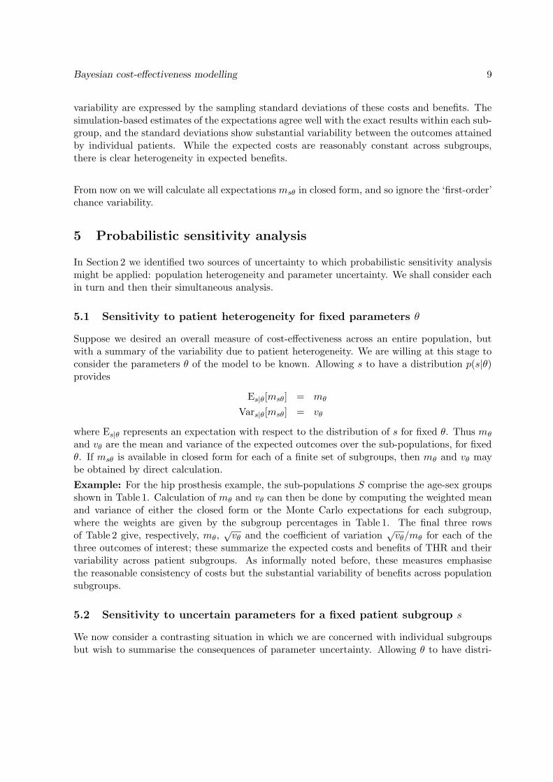
Up until now we have assumed that any available evidence (e.g. on the revision hazard) canbe summarised as a prior distribution whose influence is assessed by propagating uncertaintythrough the model using ‘forward’ Monte Carlo methods. This two-stage process can be in-tegrated into a single analysis in which the posterior distribution arising from a data-analysisfeeds directly into the cost-effectiveness without an intermediate summary step. This corre-sponds to a full Bayesian probability model and requires Markov chain Monte Carlo rather thansimply Monte Carlo techniques, since in effect the evidence from the data has to be propagated‘backwards’ in order to give the uncertainty on the parameters, and then ‘forwards’ throughthe cost-effectiveness model: a schematic representation is shown in Fig. 2.

O’Hagan and colleagues have illustrated this technique for evidence from a single trial and asimple cost-effectiveness model [22] [23] [24], while Fryback and colleagues [25] provide a furtherexample of a posterior distribution being used as a direct input to probabilistic sensitivityanalysis. The potential advantages of this integrated approach over the two-stage process arediscussed in Section 6.3.

The common situation in which evidence is available from a variety of sources demands a morechallenging statistical analysis. If the evidence comprises a set of similar trials then a standardBayesian random effects meta-analysis may be sufficient [26] [27]. In more complex situationsthere will be multiple studies with relevance to the quantities in question but which may sufferfrom a range of potential inadequacies, such as being based on different populations, havingnon-randomised control groups, outcomes measured on different scales, and so on. Formalcombination of such disparate sources is fraught with methodological problems but has beenstudied under a range of labels. Cross-design synthesis [28] is a general term for pooling evidencefrom different study designs, while the Confidence Profile Method of Eddy and colleagues [29]explicitly models a range of internal and external biases that a study may exhibit. It is naturalto extend Bayesian random effects modelling to allow variance components corresponding todifferent study designs (i.e. assuming study-types are ‘exchangeable’) resulting in hierarchical


Unknownparameters

evidenceAvailable Cost−

modeleffectiveness

Predictions

interventionof effect of

Figure 2: A schematic graph showing the dependence of both available evidence and futurepredictions on unknown parameters. After taking into account the available evidence, initialprior opinions on the parameters are revised by Bayes theorem to posterior distributions, theeffects of which are propagated through the cost-effectiveness model in order to make predic-tions. An integrated Bayesian approach ensures that the full joint uncertainty concerning theparameters is taken into account.

models with a study-type ‘level’: examples include pooling randomised and non-randomisedstudies on breast cancer screening [30], and pooling open and closed trial designs [31] [32].

There are clearly a number of issues in carrying out such potentially controversial modelling,such as when to judge studies or study-types ‘exchangeable’, how to put appropriate priordistributions on variance components, and how to carry out sensitivity analyses.

We shall consider as an illustration a somewhat simple formulation of such a model. Supposewe have a set of studies that are each intending to estimate a single parameter δ but, due todifferences in populations studied and so on, any particular study (if carried out meticulously)would in fact be estimating a biased parameter δ + δh. Here δh is the ‘external bias’, and astandard random effects formulation might then assume δh ∼ N(0, σ2

h) (note that the meanwould not necessarily be 0 if we suspected systematic bias in one direction). However, supposedue to quality limitations there is additional ‘internal bias’ in the study, so that the trueparameter being estimated is δ + δh + δb. Then we might assume δb ∼ N(0, σ2

b ) if we did notsuspect the internal bias would favour one or other treatment. Overall, we are left with arandom effects model in which, for study i, the data is estimating a parameter

δi ∼ N(δ, σ2h + σ2

bi)

∼ N(δ, σ2h/qi)

where qi = σ2h/(σ2

bi + σ2h) can be considered the ‘quality-weight’ for each study, being

the proportion of between-study variability unrelated to internal biasing factors. Thus a high-quality randomised trial might have q = 1, while a non-randomised study may be downweighted


by assigning q = 0.1.

Estimates or prior distributions of the between-study variance σ2h and the quality weights qi

might be obtained from a possible combination of empirical random-effects analyses of RCTs ofthis intervention, historical ‘similar’ case studies, and judgement. Of course, sensitivity analysisto a range of assumptions about the quality weights can be carried out, as illustrated in thefollowing example.

6.2 Example: evidence synthesis for comparison of revision rates

In order to illustrate the trade-off between increased costs and benefits, we shall compare thecost-effectiveness of the Charnley prosthesis with a hypothetical alternative cemented prosthesescosting an extra £350 but with some evidence for lower revision rates. We assume that all othercosts (operating staff/theatre costs, length on hospital stay, X-rays etc.) are the same for bothprosthesis types, and that the same method of QALY assessment is applicable for both typesof prosthesis.

For illustration, we assume that the revision hazard for our hypothetical alternative is similar tothat for the Stanmore prostheses (a popular alternative to the Charnley in practice). Evidenceon the relative revision hazards for the two prostheses is limited. The report by NICE on cost-effectiveness of different prostheses for THR [12] cites three sources providing direct comparisonsbetween Charnley and Stanmore revision rates:

1. The Swedish Hip Registry [17] provides non-randomised data submitted from all hospitalsin Sweden from 1979, with record linkage to further procedures and death. Nine-yearfollow-up results are used for around 30,000 Charnley and Stanmore prostheses.

2. A UK Randomised Controlled Trial (RCT) [33] randomised around 400 patients to Charn-ley or Stanmore and reported a mean follow-up of 6.5 years.

3. A Case Series [34] of around 1200 patients in a single hospital with a mean follow-up of8 years.

The available evidence from these three sources on revision hazards for Charnley and Stanmoreprostheses is summarised in Table 4.

We assume the following model for pooling evidence on the revision hazard ratio for Stanmoreversus Charnley prostheses. Let Nik and rik denote the total number of patients receiving pros-thesis i (1=Charnley, 2=Stanmore) in study k, and the number requiring a revision operation,respectively. We assume rik is binomially distributed with proportion pik, Hik is the cumulativehazard up to the mean follow-up, so that log(− log(1−pik)) = log Hik. Assuming a proportionalhazards model, with hazard ratio HRk for Stanmore versus Charnley prostheses, leads to thefollowing likelihood:

rik ∼ Binomial(pik, Nik), i = 1, 2

log(− log(1 − p1k)) = log H1k


Table 4: Summary of evidence on revision hazards for Charnley and Stanmore prostheses:hazard ratios < 1 are in favour of Stanmore.

Charnley Stanmore Estimated

Number of Revision Number of Revision Hazard Ratio

Source patients rate patients rate (HR) (95% int.)

Fixed effects model

Registry 28,525 5.9% 865 3.2% 0.55 (0.37–0.77)

RCT 200 3.5% 213 4.0% 1.34 (0.45–3.46)

Case Series 208 16.00% 982 7.00% 0.44 (0.28–0.66)

Common effect model

.52 (0.39–0.67)

Quality weights [Registry, RCT, Case Series] Random effects model

[1, 1 ,1] 0.54 (0.37–0.78)

[0.5, 1, 0.2] 0.61 (0.36–0.98)

[0.1, 1, 0.05] 0.82 (0.36–1.67)

log(− log(1 − p2k)) = log H2k = log H1k + log HRk

Placing uniform prior distributions over log H1k and HRk gives the ‘fixed effects’ estimates ofthe hazard ratio for each source shown in first three rows of Table 4, revealing reasonable concor-dance between the non-randomised studies but with the randomised trial showing some evidenceagainst the Stanmore. Forcing a common hazard ratio leads to the registry overwhelming theother sources (row 4 of Table 4).

The random-effects analysis with quality weights described in Section 6.1 leads to the model

log HRk ∼ N(log HR,σ2

h

qk

)

where HR is the overall estimate of the revision hazard ratio pooled across studies.

Three studies do not provide sufficient evidence to accurately estimate the between-study stan-dard deviation σh, and so substantial prior judgement is necessary. We would expect consider-able heterogeneity in revision rates between studies, even if they are internally unbiased, and soassume σh has a normal distribution with mean 0.2 and standard deviation 0.05, correspond-ing to expecting ±50% variability in true hazard ratios between studies, with 95% uncertaintylimits of 20%–80% variability. The results of a random-effects analysis with all quality weightsassumed to be 1 are shown in row 5 of Table 4, again showing the domination of the registrydata.

Our knowledge of the potential biases of registries and case series suggest downweighting thenon-randomised evidence. As a baseline assumption for the quality weights we take qk equal to


0.5, 1.0 and 0.2, respectively, for the registry, RCT and case series studies. This corresponds toassuming that ‘bias’ in the registry and case series studies leads to a 2-fold or 5-fold increase inthe revision rate variance, respectively, over and above the between-study variability expectedfor RCTs. Row 6 of Table 4 shows that the hazard ratio is still estimated in favour of theStanmore but that the 95% interval now only just excludes 1. As a further sensitivity analysiswe take qk equal to 0.1, 1.0 and 0.05, respectively, which leads to an equivocal result withsubstantial uncertainty (final row of Table 4).

6.3 Comparison of integrated Bayesian and two-stage approach

The ‘integrated’ approach to evidence synthesis and cost-effectiveness analysis simultaneouslyderives the joint posterior distribution of all unknown parameters from a Bayesian probabilitymodel, and propagates the effects of the resulting uncertainty through the predictive modelunderlying the cost-effectiveness analysis. In contrast, the ‘two-stage’ approach would firstcarry out the evidence synthesis, summarising the joint posterior distribution parametrically,and then in a separate analysis use this as a prior distribution in a probabilistic sensitivityanalysis in the cost-effectiveness model.

Advantages of the integrated approach include the following. First, there is no need to as-sume parametric distributional shapes for the posterior probability distributions, which maybe important for inferences for smaller samples. Second, and perhaps most important, the ap-propriate probabilistic dependence between unknown quantities is propagated [35], rather thanassuming either independence or being forced into, for example, multivariate normality. Thiscan be particularly vital when propagating inferences which are likely to be strongly correlated,say when considering both baseline levels and treatment differences estimated from the samestudies.

Disadvantages of the integrated approach is its additional complexity, and the need for fullMarkov chain Monte Carlo software. The ‘two-stage’ approach, in contrast, might be imple-mented in a combination of standard statistical and spreadsheet programs.

7 Incremental cost-effectiveness

7.1 Theory

Suppose we have cost-effectiveness models for two interventions. For fixed parameter values,let the expected outcomes for intervention i = 1, 2 decompose into expected costs and benefits

mθi= (m

[C]θi , m

[B]θi ). Then the incremental expected costs and benefits of intervention 2 over

intervention 1 are ICθ = m[C]θ2 −m

[C]θ1 and IBθ = m

[B]θ2 −m

[B]θ1 . Many authors [36] [37] [38] [22] [39]

[25] have argued that statements of cost-effectiveness should be based on the joint distributionof ICθ and IBθ with respect to p(θ), the joint distribution for all uncertain parameters inthe models. In particular, a plot of the joint distribution of ICθ and IBθ can be particularlyinformative.

A traditional summary of the comparison between two treatments is the incremental cost-


effectiveness ratio (ICER) ICθ/ IBθ which, for fixed θ, is the expected additional cost per unitadditional benefit. However, when uncertainty about θ is acknowledged, inference on the ICERis hampered by the possibility that IBθ=0, and hence the ICER is infinite. A solution is to usethe concepts of ‘net benefit’ and ‘cost-effectiveness acceptability curves’.

For example, suppose K is a given threshold cost per unit benefit, in that the health careprovider is willing to pay up to K for an additional unit of benefit. Then, for fixed parametersθ, the net benefit from the new intervention is

βθ(K) = K IBθ − ICθ.

The distribution of βθ(K) for fixed K provides a variety of summary measures [23]. For example,Eθ[βθ(K)] is the expected net benefit, and Claxton [40] argues that intervention 2 should bechosen if this expectation is positive, without regard to ‘statistical significance’. Perhaps amore flexible approach is to calculate Q(K) = pθ[βθ(K) > 0], and plot this against K toproduce a cost-effectiveness acceptability curve (CEAC). Further discussion and examples ofthese concepts have been provided by others [36] [37] [38] [22] [39] [25].

7.2 Example: Comparative cost-effectiveness analysis of two different hip

prostheses

We now compare expected costs and benefits by running the Markov model for each of theCharnley and Stanmore prostheses, with appropriate allowance for uncertainty and heterogene-ity. As before we assume the distribution given in Eqn. (8) for the Charnley prosthesis hazard(now denoted h1); for the hypothetical alternative prosthesis we estimate the revision hazard ash2 = h1 ×HR, where the hazard ratio HR is estimated simultaneously with the Markov modelusing the model for evidence synthesis based on comparison of Charnley and Stanmore revisionrates described in Section 6.2.

Table 5 summarizes the expectation and variability due to parameter uncertainty of the incre-

mental costs (ICθ = m[C]θ2 − m

[C]θ1 ) and quality of life benefits (IQθ = m

[Q]θ2 − m

[Q]θ1 ) of using the

alternative prosthesis rather than the Charnley both for specific patient subgroups and alsoaveraged over all patients. Note that similar summaries are possible for life expectancy. Table 5also gives the median of the distribution of the incremental cost-effectiveness ratio (ICER =ICθ / IQθ): note the preceding discussion on the difficulty of giving interval estimates for thisquantity when IQθ=0 is a plausible value. The additional benefit from the alternative pros-theses clearly decreases with increasing age, while the expected cost changes from favouringthe alternative to favouring Charnley with increasing age. This leads to a negative ICER foryounger ages.

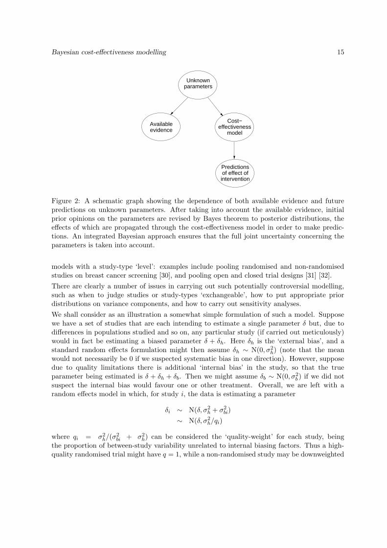
The full joint distribution of ICθ and IQθ is shown in Fig. 3 for each subgroup and averagedover all patients. Values within the bottom right quadrant indicate both lower cost and greaterbenefit arising from the alternative prosthesis, and hence a strictly dominating intervention.The diagonal dashed line in each plot indicates the pairs of values of ICθ and IQθ yieldinga zero expected net benefit for Stanmore if the health care provider is willing to pay up to


Table 5: Summary of results of comparative analysis of cost-effectiveness for a hypotheticalalternative versus the Charnley prostheses, using quality weights of [.5, 1, .2] for weighting theregistry, RCT and case study evidence respectively.

ICθ (£) IQθ (QALYs) ICER

Subgroup mean sd mean sd median Q(6,000) Q(10,000)

Men

35-44 yrs −90 256 0.136 0.063 −846 0.92 0.94

45-54 yrs −28 216 0.113 0.053 −457 0.91 0.93

55-64 yrs 71 156 0.081 0.038 581 0.87 0.92

65-74 yrs 216 75 0.038 0.018 5,190 0.55 0.77

75-84 yrs 279 40 0.020 0.009 13,220 0.04 0.26

>84 yrs 303 26 0.013 0.006 21,830 0.00 0.02

Women

35-44 yrs −63 238 0.127 0.059 −691 0.91 0.94

45-54 yrs −14 206 0.109 0.051 −349 0.90 0.93

55-64 yrs 66 161 0.083 0.039 537 0.87 0.92

65-74 yrs 209 79 0.040 0.019 4,710 0.60 0.80

75-84 yrs 274 43 0.021 0.010 12,030 0.07 0.34

>84 yrs 297 28 0.015 0.007 18,790 0.00 0.06

Overall 183 90 0.048 0.022 3,246 0.73 0.85


K = £6, 000 for each additional QALY of benefit (i.e. βθ(6, 000) = 0); the proportion ofpoints in the joint distribution below this line represents the probability of cost-effectivenessfor the alternative prosthesis for K = £6, 000 (i.e. Q(6,000) = pθ[βθ(6, 000) > 0]). Likewise,the diagonal dotted line represents pairs of values (ICθ, IQθ) yielding a zero expected netbenefit for K = £10, 000 (i.e. βθ(10, 000) = 0), and the proportion of points below the dottedline correspond to Q(10,000), the probability of cost-effectiveness for the alternative prosthesisat £10, 000 per QALY. The cost-effectiveness probabilities Q(6,000) and Q(10,000) for eachsubgroup and averaged over all subgroups are summarized in the final two columns of Table 5.

We see that, for K = £10, 000, the probability that the alternative prothesis is the cost-effectiveoption is around 80% or more for both men and women under 75, but declines rapidly thereafter.For K = £6, 000 the threshold is around 65 years.

Fig. 4 shows Q(K), the probability of cost-effectiveness for the alternative prosthesis if thehealth care provider is willing to pay up to £K for each additional QALY of benefit, plottedagainst K for each subgroup and averaged over all subgroups. The solid line is based on theresults of the analysis reported above; the other curves in each plot indicate the sensitivity of thecost-effectiveness probabilities to various model assumptions. Specifically, we have re-run themodel using downweighted evidence from the non-RCT studies on the revision hazard ratio forStanmore versus Charnley. This was achieved by using quality weights qs equal to 0.1, 1.0 and0.05, respectively, for the registry, RCT and case series studies. Sensitivity to the assumptionthat benefits are to be discounted by δb=6% per annum was also examined, by re-running themodels using a reduced health discount rate of 1.5% per annum.

The results indicate that cost-effectiveness depends strongly on age (and to a lesser extenton sex), which suggests that economic evaluations should be made separately for the differentsubgroups. However, there is considerable sensitivity to the choice of quality weights used inthe evidence synthesis, with further downweighting of the non-randomised evidence leading toconsistently lower cost-effectiveness probabilities for the alternative prothesis in all age andsex groups: the probability of cost-effectiveness does not rise above 75% for any value of Kconsidered. This is to be expected, since the RCT provided less favourable evidence of reducedrevision rates for the alternative prothesis than did the non-randomised studies. Sensitivity tothe health discount rate is not particularly strong in general, but is more apparent for older agegroups.

It is of interest to compare the two-stage approach, which separates the data analysis andevidence synthesis from the cost-effectiveness analysis, to the integrated approach describedabove (Section 6.3). We applied the two-stage approach using the 3 data sources (Registry, RCTand Case Series) to estimate the revision hazard for Charnley (rather than using the values forh derived in Section 4.2) as well as the hazard ratio. Independent normal distributions werethen assumed for the log hazard for Charnley and for the log hazard ratio. The results werevirtually identical to the integrated analysis - the posterior standard deviations are about 1-2%smaller under the two-stage approach and the CEA curves were very similar. The correlationbetween the log hazard for Charnley and the hazard ratio is also quite small (about -0.15) inthe model, which would explain the similar results from the two approaches.


8 Conclusions

In this paper we have attempted to explore a range of concerns that arise in cost-effectivenessmodelling, but acknowledge that there are a number of issues that we have passed over. Inparticular, we have not explored the sensitivity of the conclusions to ‘ignorance’ about thestructure of the appropriate model as discussed in Section 2: alternative models that could beused in this context include survival-type models with competing risks. It is vital to admit thateven a reasonably complex model, such as that investigated in our example, cannot be assumedto be realistic and must be subject to careful criticism [41] [42].

As attempts are made towards evidence-based health policy in both clinical and public-healthcontexts, models will inevitably become more complex and, while the methods described in thispaper may appear complicated, we feel that techniques such as these may well become common-place in the future. If decisions made with the help of such analyses are to be truly accountable,it is important that the models and methods are transparent, easily updatable, and can be runby many parties in order to check sensitivity. Models implememented in spreadsheet programshave some of these characteristics, although personal experience suggests that such programsare very clumsy in handling multi-dimensional arrays, and their expressions of complex for-mulae are quite opaque. Thus the supposed transparency of popular spreadsheet programsmay be somewhat illusory, and we feel that user-friendly Bayesian simulation programs couldcontribute substantially to the field.

The hip replacement data and Winbugs code to fit each of the models discussed here areavailable from www.mrc-bsu.cam.ac.uk/bugs/examples.

Acknowledgements We are very grateful to Andy Briggs and Mark Sculpher for providingtheir original model and for helpful discussions, and to Andrew Thomas for rapidly adaptingthe Winbugs program to be able to handle complex logical dependencies.


..

.

..

...

.. .

.

.

.

.

..

..

.. .

...

..

.

.....

...

.

...

.

.

... .

.

..

. ...

.

... ..

.

...

..

.

...

.

.

.

..

.

...

.. .

..

.

....

.....

...

. .

..

...

..

.

.

.

. ..

.. .

..

..

....

..

.

..

.

.

..

.

...

.

..

.

.. ...

.

.

.

.

..

..

..

.

.. ...

.

.

..

..

.

...

.

..

.

.

.

... ..

.

.

.

.. ..

....

.

..

.... .

.

.

.

. .

....... .

.

...

..

.. .

.

.

.

....

.....

.

...

.

...

..

..

.

.

....

..

.

.

.

..

.. ..

...

..

..

..

..

..

.

..

..

..

..

.. .

....

..

..

.

..

..

..

....

..

.

.

..

. .

.

..

...

.

.

.

.

. . ...

.

...

.

.....

.

..

.. ..

.

.

..

..

.

..

.

..

..

.

.

..

.

.

.....

.

..

..

.

.

...

...

.

..

.

..

.

.

..

..

. .

..

....

..

. .

.

..

..

.

.

. ..

...

.

.

.....

....

...

..

.

.. .

...

.. .

.

..

...

..

... .

.

..

.

....

..

......

.

.

..... .

..

.

.. .

...

.

..

. .

.

.

..

..

..

.

..

..

..

..

.

.

.

.

..

.

..

.

... ..

.

.

.

.

..

..

.

.

. ..

...

.

..

.

. .....

.

.

....... ..

.

.

....

..

.

.

.

. ..

.

. ..

.

. ..

..

..

.

..

.

..

...

..

..

.

.

...

..

..

...

.

..

.

.. ..

... .

...

. ...

.

.

.. ..

.

..

.

..

...

. ...

..

.

.

..

...

..

.

..

...

.

.

...

..

.

..

.

..

.

... .

..

..

.

..

..

.

.

..

..

....

.

..

.

.

..

.

.

..

..

.

....

.

.

...

..

.

.

.

..

..

.

..

. .

.

..

......

.

.

.

..

...

.

..

...

.

..

.

...

..

..

..

.

.

..

.

.

... .

..

.

...

.

.

.

..

..

.. .

.. .

...

... .

.

.

.. ..

.. .

.

..

......

..

. ...

.

..

..

.

...

.. ..

...

.

...

....

..

..

.

.

.

.. .

.

..

...

..

.

..

.

...

..

.

..

.. .

.

.

. ..

...

..

.

.

.

..

...

...

...

... .

.

..

.

.

..

.

.

.

..

.

...

..

.

.

...

...

.

. .

. .

.

.

.

..

.

..

..

.

...

.... .

.

.

.

.

.

..

.....

...

.. ...

..

QALY increment

Cos

t inc

rem

ent

-0.1 0.1 0.2 0.3

-100

0-5

0050

010

00

Women, <45 yrs

...

....

. ....

.

.

..

...

... .

.

.

...... ..

...

.

....

.

...

.

..

.

... .

.

.. .

...

...

..

..

..

..

.

..

..

..

...

..

..

...

. .

..

..

..

..

. .

..

....

.

.

.. ..

......

. . ..

. .

.. ..

.

..

. ........

..

..

..

.

.

.

..

...

.

......

.

...

..

. .. .

..

..

..

.. ..

..

..

...

....

.

...

.....

.

.

..

. . ..

. ....

.

.. ..

.. .

.

..

... .

.... .

.

.

..

......

. .

.

..

.

..

..

..

.

..

...

...

..

.

.. . .

.

...

.....

.. .

.

.. .. .

...

.

.. .

....

...

...

..

..

..

..

.

..

...

.

..

.

..

..

.

..

..

.

. ...

...

..

.. ..

....

.

. ..

...

...

.

.

.

.

.

.....

...

.

. .

.. .

. .

. ..

..

.

..

.

...

. ..

.

..

.. ..

.

...

.

..

. ..

. ...

...

.

.

... .

.

....

...

. .

.

...

. ...

..

...

.. .

..

....

...

.

... ..

.

... .

.

..

.

... ...

..

.

....

..

.. .

..

.

...

..

...

....

.

.

.

.

..

... .

.

..

.

. .. ..

..

.. ..

..

. .

. ..

. ...

...

..

....

.

.

. . .....

...

.

....

..

.

.

.

. ..

.

...

..

.. .

...

.

..

.

..

....

..

..

.

. ...

...

...

.

..

.

. ...

.

..

....

.... .

.. ... .

...

..

...

......

.

.

..

.... .

.

..

...

.

.

.

..

...

..

.

..

...

. .

.. ..

..

..

.

...

.

..

... ..

...

.

..

.

.

...

.

.

.. ..

.

.

...

..

.

..

..

...

..

...

... . ...

.

..

.

..

....

.

.

.. ..

...

..

.. ...

.

.

. . . .

..

...

.

..

.

...

.

.

.

..

..

...

. . ....

. . . ..

.

.. ..

....

. ......

...

. ....

...

.

.. .. ...

..

..

...

... .......

..

...

.

... ..

.

..

..

.

..

.

...

..

...

.

.

. ..

...

..

.

.

.

..

..

.

...

. .......

....

..

..

..

.

.

...

...

.

..

..

.

..

. ...

..

.

....

....

..

......

..

.

.

.

..

....

... . ... .

...

QALY increment

Cos

t inc

rem

ent

-0.1 0.1 0.2 0.3

-100

0-5

0050

010

00

Women, 45-54 yrs

. .....

....

.

.

.

.

.

....

...

...

..

... ..... .

.... ....

..

.. .

. ...

..

....

.

...

... .

..

..

...

.... . ..

..

. ...

.

.

. ... ...

..

..

...

...

.

.

.. ..

.....

.. ...

...

..

..

.

.....

......

. ..

..

..

..

. ...

.

.

...

.

.

.

.. ..

..

..

.

..

..

. ... . ....

....

....

.

..

.... .

.

.

.

. .... ..

...

... ..

...... .

. .. .

..... .

. ..... .... .

.

.

.. ..

...

.

....

..

.. ..

..

...

.

..

...

...

.

.....

..

.... ... .

.

..

.....

....

..

.

...

.

...

...

.

..

.. ..

.....

..

. ..

......

. ...

... ..

..

.

..

.

..

.

..

.

.

.

.....

..

.

.

.....

. ... .

..

..

.

.

.... .

..

... . . .

...

..

..

..

..

. ..

. ..

..

. .. ..

. ....

..

..

.

.... .... .

...

. ..

.

...

..

...

..

...

.....

.

...

...

....

..

.. ..

...

...

. ..

.. .

..

.... .

... . ..

.

.. ...

.

..

.

.... .

..

....

..

.....

... .

.... .

.. .

..

... ..

... .... ....

..

..

....

..

.......

....

..

.

..

.... .

. ..

....

...

..

..

..

....

..

...

.. .

..

....

..

.. ..

..

.

...

..

.. ..

...

.

. .

....

..

...

...

.

..

...

.

..

.

..

.

.....

. ..

..

..

..

.

. .

.

.. .. ..

.. .

.

..

.

.....

.

..

...

.

...

..

..

.. ..

....

. ..

..

.. ....

..

.

.

....

..

.

... .

..

...

.. .

..

..

..

. ...

... .

..

.

...

.. .

..

..

. . .. . .

...

. .. ..

.

.. ..

.. .

.

.....

. ..

.....

.

...

..

..

.

... ..

...

....

. . . ... .

.

..

....

.

.... .

...

..

....

.. ......

.

.

.. .

..

.

..

..

..

..

..

...

.. .... ..

...

.

..

..

..

..

...

...

.

..

.. .

..

.....

. .. .. .

.. ... ....

...

..

.

.

.

... .....

....

..

...

QALY increment

Cos

t inc

rem

ent

-0.1 0.1 0.2 0.3

-100

0-5

0050

010

00

Women, 55-64 yrs

... .... .......

........ ..

.. ............ ... ... ...

.. . ... .... ...

.......

... .

...

.. .. . ..

. .. .. ..

... .. ...

. ...

. ..

....

.... ...

.. .

.. ......

... .. ...

. .. ..... .. ..

.

... .....

..

.....

.. ... .. ..

...

..

.... .........

.....

........

..

. .....

........ .... ....

. ....

........ .. . .... .

..

..

..... .

. .. .......

.... .. .... .

...

..... . ..

.... .. ....

.

... .... ..

.. .

...

.

...

....

. ...

..... .

........

..

..........

....

...

......

....... ... . .....

.....

.. ...

.. ..

. ....

.. .. .... ... .

.......

... .. ......

........

.

.. ........

...........

...

.....

....... .

.. ....... ..

..

... ....

...

.....

.... .

...

.... ...

. . .. . .. ....

..

.. .. .. .

... .... ..

..... .... .........

. ...

..

. . ..

.. . ..

........ .

. .. .

. ..

. . ... . ...

. . .. ..

... ..........

... ...... ...

..

.. ......

......

...

.. .

.. .

....... .... ...

... ....

.. ......

..... ..... ... ..... .. ..

..

...

... ..

......

.. .

...

..

.. ... .. .

... . .......

..

......

... ... . ........ ..

..

. ....... ....

.... .....

. .... ......

..... ... . ... ....

.........

... ...

.. . . .. ..

......

...... .. ...

.. ..

....

.. ... .

...

... .

. ...... ..

.

......

... .

... ...

...

... .....

........ ..

.... .

....

.. .

....

... ... ..

... .

... ... .......

..

. . .

.. ....... ......

QALY increment

Cos

t inc

rem

ent

-0.1 0.1 0.2 0.3

-100

0-5

0050

010

00

Women, 65-74 yrs

........... ............... ...... ... ... ........

... ................ ......... ............................... ........ ......... . ...... ............ ................. ... ..... ........

....... .......... .

.........

. .. .......... ... ............. ................ .. ...... ... ..

........

. .. ......... ...... . .

........... .

....... ..... ... .

...... ... .. ............ ......

.... ........ ...... ...

. ......... ...........

.. ......... ..... .. ..... ...... ....... .. ........... .......... ....

........

. .......

..... .... .... ... ...

......... . ..... .....

..... ........... .... .... ......... .... ...... ..... ..... ........ .... .......

.. ........... .. ...

... ..................... ... ........... ..

.... ........... .. .........

.. ............. .......... .......... . ......

.. ....... .... . .......

.. .... .......... ... ............ .......

...... .... ......... .....

...... .... .... .....

........ ........ .... ... .......... ....... .... .. .... .......... ........

...... ..... .....

. ..... .......

.... ..... . .......... ........ .......... .....

....

..... .. ........ .... ..... ...... .... ................ . .

QALY increment

Cos

t inc

rem

ent

-0.1 0.1 0.2 0.3

-100

0-5

0050

010

00

Women, 75-84 yrs

... ........... .... ................... .... ........ .... ............. .................... ..... ............ ........................... ............................................. .................. ........

........ ................

..... ................ ........... ........................................ ................ ........ .... ...... ............................... .... ......... ..... ............................. .................... .........

. ............ ...... ...... ...... .............................. ...................... ................ ........................................

.............. ...... ..... ............. ... ...

...... .....................

. .......................... ............ ........ ................ ...... .... ... ...................................

............ ........... ............. .........

...................... ... ............................................. .... .......................

. ... ..... ........... ........................... ........

....... ..... .............

................ ...

QALY increment

Cos

t inc

rem

ent

-0.1 0.1 0.2 0.3

-100

0-5

0050

010

00

Women, >84 yrs

..

.

...

.. ..

.

.

.

.

.

..

..

...

.. .

..

.

....

.

..

.

.

...

.

.

... .

.

..

.. ..

.

...

..

.

. ..

..

.

...

.

.

.

..

.

...

...

.

..

..

..

... ..

.

..

..

..

...

...

.

.

....

... .

. .

....

..

.

..

..

... .

.

...

..

.

..

...

.

.

.

.

.

....

.

.

.... .

.

..

..

.

... ..

.

.

.

.... ..

..

.

....

.. .

.

.

.

..

.....

.

.

..

....

....

.

....

.

.. .

.

.

.

....

.. .. .

.

. ..

.. .

.. .

..

.

.

. .

.

.

...

.

.

..

.

.

..

..

.

.

.

..

..

..

...

..

..

...

.

.

..

..

..

..

.

. .

..

..

..

....

..

.

.

..

..

.

..

...

.

.

.

.

....

.

..

..

.

...

. .

.

...

. ...

.

..

..

..

.

.

..

..

.

..

.

.

.

.

.. ..

.

. .

....

..

....

.

..

.

..

.

...

..

.

.

.

.... .

.

. ..

.

..

..

.

....

...

.

.

..

...

. ...

..

.

..

.

.. .

....

..

.

. .

..

...

. ..

.

.

. .

..

.

..

..

.......

.

.

.... .

..

..

.... .

..

.

. .

.

...

..

..

.

..

...

....

..

.

.

..

..

.

. .

...

...

.

.

.

..

..

. ..

.. .. .

..

...

..

.

.

.

. ...

....

...

.. ... .

.

.

.

. ..

.

..

..

....

.

..

.

.

.

.

.

....

..

.. ..

.

..

..

..

...

.

..

...

.

..

. . .

.

... .

.

..

..

....

. .

.

..

...

..

. .. .

.

.

..

...

..

.

...

..

.

.

.

..

...

..

.

.

..

.. ..

..

..

.

.

..

.

.

..

.

..

...

.

.

..

.

.

.

.

.

.

..

..

.

...

..

.

...

..

.

.

...

...

.

.

. .

..

..

...

..

..

.

..

...

.

.

.

...

.

..

...

...

.

.

..

.. ..

..

..

. .

..

.

.. .

.

.

.

..

.

..

. .. . .

..

.. .. ..

.

.. .

.

.

..

...

..

..

.

...

... .. .

. .

.

. ..

..

...

...

.

.

...... .

.

..

.

.

.

.

..

.

.

..

..

..

...

.

. ..

..

.

..

.. .

.

.

. ..

..

.

.

.

.

.

.

..

..

.

...

.... .

. ..

....

..

.

.

.

..

.

. ..

..

.

.

...

...

.

..

.

...

.

.. .

.

...

.

..

...

...

.

.

.

.

.

..

. ... ..

....

.. .

.

.

QALY increment

Cos

t inc

rem

ent

-0.1 0.1 0.2 0.3

-100

0-5

0050

010

00

Men, <45 yrs

..

.

....

. ...

.

.

.

.. ....

....

.

..

.

....

..

...

...

..

....

..

.

....

.

..

.

...

...

..

..

..

..

.

. .

.

...

...

..

...

.

.....

...

.

..

..

..

.

...

.

.

...

..

... .

.....

..

..

..

.

...

..

....

.. ..

..

.

.

.

.

.

..

. .

...

.

...

.

.

..

...

...

...

..

......

..

.

....

...

.

.

..

.

... ..

.

.

..

. . ..

.. .

...

.. .

..

..

..

.

.. ..

..

...

.

.....

.

..

...

.

.

. ..

....

.

.

.

.

....

....

.

..

.

.

........

.

....

...

....

.

.

...

..

... ..

...

..

.

.

..

.

.

..

.

...

.

..

.

...

.

..

..

..

...

...

..

.. ..

.

...

..

. ..

.

..

.

.

.

.

..

.

.

..

...

.

..

..... .

.....

..

.

.

.

.

.. .

..

..

.. .

. ...

...

.

..

..

.

.

. ..

...

.

.

..

..

.

...

...

...

.

....

...

..

.

..

...

..

....

.. .

..

...

. .

....

...

.

... ...

..

.

....

..

.. .

..

.

.

..

..

..

.

..

.. ..

..

..

..

.

..

..

.

. .. ..

..

...

.

.

...

.... ...

..

..

... ..

.

.....

...

..

..

. ..

.

. .

..

.

...

..

...

....

...

.

.

.

.

..

...

..

.... .

...

. ..

. ..

.

..

...

..

. .. .

.....

...

.. ..

.

.

. ..

..

...

....

. ..

.

..

.... .

.

..

...

.

.

..

.. ..

..

.

..

.

....

.. ..

....

.

.

...

......

....

.

.

.

.

.

..

..

.

....

.

.

...

..

.

..

....

.. .

...

.

... .. .

.

..

.

..

...

.

..

...

.

.

..

...

..

.

.

.

.

.. ..

..

....

..

.

...

.

.

.

..

..

...

. . ..

..

. ....

.

.. ..

....

..

...

..

...

...

.. ..

..

...

. .. .

. ...

..

. ..

...

....

..

.

.

..

.

...

... .

...

.

..

...

.

..

.. .

.

.

. ..

...

..

..

..

.

..

.

...

... ..

...

....

...

.

..

.

.

...

..

.

.

..

..

..

.

..

.

. ..

.

. ..

....

..

..

. .

. ..

..

.

.

.

...

....

..

..

.. ...

.

QALY increment

Cos

t inc

rem

ent

-0.1 0.1 0.2 0.3

-100

0-5

0050

010

00

Men, 45-54 yrs

..

.... .

. ..

.

.

.

.

.. .......

...

.. ...

......

....

..

...

.. .

... .

.

...

...

...

..

....

..

.

...

.. ....

.

.. . .....

....

.

...

..

..

....

.

.

....

.... .

.

....

...

..

..

.

.......

.. . .. ...

.

.

.

.

.... .

..

.. .

.....

. .... . .

..

..

...

.. ..

..

....

....

.

..

.....

.

.

.

.... .. .. .. .

..

..

....

.

.

.

....

..

.....

...

...

..

.. .

...

..

. ...

.....

.

.....

.. .

..

..

...

. ....

.... ..

. ....

.

...

.. .

.......

..

..

..

..

.

..

...

.

..

.. .

..

...

..

.

.. .. .

.

...

. ...

.. .. ....

.

..

...

...

.

.

. .....

.... ..

.. ...

..

...

..

..

.... .

..

.. . ... ...

.

. ... .

... .

...

..

....

.

...... ..

.

.

...

...

.

..

...

.. .....

...

. .

..

.... ....

. .. .

..

.....

.. .

. ..

.. .

...

...

.

....

...

.. . ..

..

..

....

.

.

..

.

.....

.....

.

..

. .. .

. ... ..

..... .

...

.....

... ....

..

. ...

..

...

.

....

.

....

.

..

.

. .

.

..

....

...

...

.

..

...

...

.

..

..

.

... ...

.

... .. ..

..

...

...

.

..

.. ..

......

.

..

.....

.

...

...

.

......

..

.

..

.

... .

.. ..

...

..

...

.

..

.. ..

. ....

..

..

....

.

.. .

..

.

. ..

..

..

..... ...

....

..... ..

..

.

.

.

....

..

... .

.

..

......

.

.

.

..

..

..

..

..

..

.

. ..

.

..

..

..

...

. ..

..... ... .

....

...

...

..

... ....

..

....

..

..

... ..

.....

.... .. .. .. .

..

..

..

...

...

..

...

.

...

...

..

...

.

.

.. .

...

..

. .

..

..

..

...

. .......

.. ..

.. .

..

...

...

...

.

.. .

..

..

. .

..

..

.

...

.. . .

. .... ... .

..

.

.

.

..

. . .. . . . ... . .

.

..

QALY increment

Cos

t inc

rem

ent

-0.1 0.1 0.2 0.3

-100

0-5

0050

010

00

Men, 55-64 yrs

... . .......

..

.. .

. ...... .... ... ........... .

...... ... ..

.. .. ...... ..

... .. .

... .... .....

........ .....

. ...

.. . ....

... .......

...... .

....

..... ......... ... .

...

..... .... ... .

...... .....

... ..... .......

....

........

..

.

... ... .... . ........ .

..

. ....... . .

. ..... ..... .

.. .... .. ..

..

.. ...

..... ...

..

..... . ....

......

. ..........

..... ...

. ...

....

.... .

. ...... .

. ... .. .. .. ........ ...

.....

...

....

..

..

. .. .. ... . ............ . ..

..

... ........

. ...

..

... . . ......... . .. .. .

.......

..

......

.. ....

....... .....

.......

.... ....... ..... . ....

.....

. ..

..... . ... ... ..... .. ...

.. .

... ... .. .... ... .

...

. ......

.. .....

..... ... .. ..

..... ...

.... .. . ...... ..

..

..

.. . ... ..

. .

..

....... ... .........

.... .........

.. .....

.. ......

. ...

.. .

.... . .. .... ..

. ... .

....

... ........

..... . ...

..........

..

..

... ..

.. .... .... . .

..

.... ..... .

..

..

.......

. . .

..........

.....

. .. . .

. ..

....

... ....

... ...

...

... .. .... ........

.... .... .....

. ...... .......

.. ... ........... ....

....

.....

.... ..

.. ...

. .... .... ...

..

.. ....

.. ..

... . ..

........

... ... ... .. . ......

....

... .......

. .... ...

.... ..

......

...

. ..... .

. .. .... .... .

QALY increment

Cos

t inc

rem

ent

-0.1 0.1 0.2 0.3

-100

0-5

0050

010

00

Men, 65-74 yrs

... ........... ................ ....

... ............ ... ....... ..........

..... .............. ............ ....... ...... .....

. .... ......

... ..... .. ... ... .. .............. ...... ... ....

....... ...........

. ......... .

... ........ ........ ......... ..... ..... ........ .... .. .. ........... .... ............. ................

.......... .. ... ..... .

.......................... ...........

. .....

. ...... ... ... .......... ..... .... ................. .... .... ... .............

.....

......

...

....

....... ....... .... ..........

......... ...... .....

........ ........ .... ......

.... .. ....................

. ..... ....... ............ ......... ....

... ..... ................... ... ..............

..... ... ...... .. ........ .... ......... ........ ............ . .... .... ............. .... ..

...... ........ ....... ..... ........

....

... ... .... ................ ........ ...... ........... .......

..... ....... .....

....... ....

. . ..... ...... .................. ....... ...............

.. ... ..... ....... .... ........ .......... ..... .... ... ............................... . ................ .

QALY increment

Cos

t inc

rem

ent

-0.1 0.1 0.2 0.3

-100

0-5

0050

010

00

Men, 75-84 yrs

... ...... ..

..

.. ....

... . . .. . ... ..... .

..... ... ..

.. .

.....

... ......

....

... .

...

.... ...

. . . ............

. ...

.. .....

.

... .. .....

. .....

.. .. ................

..

.. ..

.....

.......

.... .. .. ...

..

........

.....

... ..

.. ......

..

. ..... .....

........ .

..

. ........ .

. .. ... .... .

..

....... .

..... ..

....... ..

.....

. ...

.... . ...... ..

... ....

..... ...

..

... .

...

....

..

.. .. ..

. . .. .... .. .

.......

... .....

...

...

. ..

..

. ...............

.....

...

.. ....

...

.... ..... .. .

.. .....

....

.. ....

. ..... ...

.

... . ......

..

... .... ..

...

...... .

.... ...

.......

. . ...... .

.....

....

.....

. . ... .... .... .

.

. ..

.. ..... .. .. ....

....... ..... ......

....... ....

.... ...

..

.... ........

. ...

. ..

. . ... . . .....

...... ...

...

... ... .... ... ....

........

...

....... .. .

.. .

.... . .. ..

.. ..

. .. ...

...

. ......

..... .....

.....

..... ....

. ..

... ..

.. ....

.... . ..

..... ....

... . ..... ....

...

....

..

....... ..

... . ..

.. ...

.... ..

...

....

..

... .. .. ...

........ .

....

.... .... .... ..... ....

.... .....

.....

.... .... ....

..

....

... .. ...

..

....

.. ... ...

..

.. ....

...

..

... .

.

...

........

... ....

..

. ..

.. ....

.......

...

.... ..

... .... .. ......

...

..

...... .. .... ... . .

QALY increment

Cos

t inc

rem

ent

-0.1 0.1 0.2 0.3

-100

0-5

0050

010

00

Overall

Figure 3: Incremental HRQL benefits (IQθ) versus incremental costs (ICθ) for the alternativeversus Charnley prostheses, for patient subgroups and overall (note that results for men aged> 84 years are not shown due to space limitations and because the distribution of patients overage-sex groups shown in Table 1 indicates that there are no THR recipients in this subgroup).Diagonal lines indicate zero expected net benefit (βθ(K) = 0) for the alternative prosthesis forK = £6, 000 (dashed line, −−−−−) and K = £10, 000 (dotted line, ..........) per QALY.


K (in pounds)

Pr(

Cos

t Effe

ctiv

e)

0 5000 10000 15000 20000

0.0

0.2

0.4

0.6

0.8

1.0

Women, <45 yrs

K (in pounds)

Pr(

Cos

t Effe

ctiv

e)

0 5000 10000 15000 20000

0.0

0.2

0.4

0.6

0.8

1.0

Women, 45-54 yrs

K (in pounds)

Pr(

Cos

t Effe

ctiv

e)

0 5000 10000 15000 20000

0.0

0.2

0.4

0.6

0.8

1.0

Women, 55-64 yrs

K (in pounds)

Pr(

Cos

t Effe

ctiv

e)

0 5000 10000 15000 20000

0.0

0.2

0.4

0.6

0.8

1.0

Women, 65-74 yrs

K (in pounds)

Pr(

Cos

t Effe

ctiv

e)

0 5000 10000 15000 20000

0.0

0.2

0.4

0.6

0.8

1.0

Women, 75-84 yrs

K (in pounds)

Pr(

Cos

t Effe

ctiv

e)

0 5000 10000 15000 20000

0.0

0.2

0.4

0.6

0.8

1.0

Women, >84 yrs

K (in pounds)

Pr(

Cos

t Effe

ctiv

e)

0 5000 10000 15000 20000

0.0

0.2

0.4

0.6

0.8

1.0

Men, <45 yrs

K (in pounds)

Pr(

Cos

t Effe

ctiv

e)

0 5000 10000 15000 20000

0.0

0.2

0.4

0.6

0.8

1.0

Men, 45-54 yrs

K (in pounds)

Pr(

Cos

t Effe

ctiv

e)

0 5000 10000 15000 20000

0.0

0.2

0.4

0.6

0.8

1.0

Men, 55-64 yrs

K (in pounds)

Pr(

Cos

t Effe

ctiv

e)

0 5000 10000 15000 20000

0.0

0.2

0.4

0.6

0.8

1.0

Men, 65-74 yrs

K (in pounds)

Pr(

Cos

t Effe

ctiv

e)

0 5000 10000 15000 20000

0.0

0.2

0.4

0.6

0.8

1.0

Men, 75-84 yrs

K (in pounds)

Pr(

Cos

t Effe

ctiv

e)

0 5000 10000 15000 20000

0.0

0.2

0.4

0.6

0.8

1.0

Overall

Figure 4: Probability of cost-effectiveness for the alternative prosthesis for each subgroup andoverall, versus cost (£K) that the health care provider is willing to pay for each additionalQALY of benefit (note that results for men aged > 84 years are not shown due to space limi-tations and because the distribution of patients over age-sex groups shown in Table 1 indicatesthat there are no THR recipients in this subgroup). Results are shown for different choices ofquality weights qs for the registry, RCT and case series studies, and different health discountrates d, as follows: −−−−−− shows qs = (0.5, 1.0, 0.2) and d=6%; ................ shows qs = (0.5, 1.0,0.2) and d=1.5%; − − − − shows qs = (0.1, 1.0, 0.05) and d=6%; −−−−−− shows qs = (0.1,1.0, 0.05) and d=1.5%.


References

[1] Briggs AH. Handling uncertainty in cost-effectiveness models. Pharmacoeconomics 2000;17:479–500.

[2] Luce BR, Shih YCT, Claxton K. Bayesian approaches to technology assessment and deci-sion making. Int J Technol Assess Health Care 2001;17:1–5.

[3] Manning WG, Fryback FG, Weinstein M. Reflecting uncertainty in cost-effectiveness anal-ysis. In: MR G, JR S, MC W, LB R, editors, Cost effectiveness in health and medicine,New York: Oxford University Press, 1996 pp. 247–275, pp. 247–275.

[4] Spiegelhalter DJ, Thomas A, Best NG, Lunn D. WinBUGS Version 1.4 User Manual. MRCBiostatistics Unit, Cambridge, Available from www.mrc-bsu.cam.ac.uk/bugs 2002.

[5] Fryback DG, Stout NK, Rosenberg MA. An elementary introduction to Bayesian comput-ing using WinBUGS. Int J Technol Assess Health Care 2001;17:98–113.

[6] Briggs AH, Gray AM. Methods in health service research - handling uncertainty in eco-nomic evaluations of healthcare interventions. Br Med J 1999;319:635–638.

[7] Burmaster DE, Wilson AM. An introduction to second-order random variables in humanhealth risk assessments. Hum Ecol Risk Assess 1996;2:892–919.

[8] Draper D. Assessment and propogation of model uncertainty. Journal of the Royal Statis-tical Society series B 1995;57:45–97.

[9] Briggs A, Sculpher M. Markov models of medical prognosis - commentary. Br Med J 1997;314:354–355.

[10] Briggs A, Sculpher M. An introduction to markov modelling for economic evaluation.Pharmacoeconomics 1998;13:397–409.

[11] Cronin KA, Legler JM, Etzioni RD. Assessing uncertainty in microsimulation modellingwith application to cancer screening interventions. Statistics in Medicine 1998;17(21):2509–2523.

[12] NICE Appraisal Group. The effectiveness and cost effectiveness of different prostheses forprimary total hip replacement. Tech. rep., http://www.nice.org.uk 2000.

[13] Fitzpatrick R, Shortall E, Sculpher M, Murray D, Morris R, Lodge M, et al.. Primary totalhip replacement surgery: a systematice review of outcomes and modelling cost effectivenessassociated with different prostheses. Health Technology Assessment 1998;20(2).

[14] Baxter K, Bevan G. An economic model to estimate the relative costs over 20 years ofdifferent hip prostheses. J Epidemiol Community Health 1999;53:542–547.

[15] Faulkner A, Kennedy LG, Baxter K, Donovan J, Wilkinson M, Bevan G. Effectivness of hipprostheses in primary total hip replacemnet: a critical review of evidence and an economicmodel. Health Technology Assessment 1998;20(6).


[16] Malchau H, Herberts P, Ahnfelt L. Prognosis of total hip-replacement in sweden - follow-upof 92,675 operations performed 1978-1990. Acta Orthop Scand 1993;64:497–506.

[17] Malchau H, Herberts P. Prognosis of total hip replacement: revision and re-revision ratein thr. a revision-risk study of 148,359 primary operations. In: 65th Annual Meeting of theAmerica Academy of Orthopaedic Surgeons, New Orleans, USA, 1998 .

[18] Laupacis A, Bourne R, Rorabeck C, Feeny D, Wong C, Tugwell P, et al.. The effect ofelective total hip-replacement on health-related quality-of-life. J Bone Joint Surg Am Vol1993;75A:1619–1626.

[19] Palisade Europe. @RISK 4.0. Tech. rep., http://www.palisade-europe.com 2001.

[20] Decisioneering. Crystal Ball. Tech. rep., http://www.decisioneering.com/crystal_ball2000.

[21] Halpern EF, Weinstein MC, Hunink MGM, Gazelle GS. Representing both first- andsecond-order uncertainties by monte carlo simulation for groups of patients. Med DecisMak 2000;20:314–322.

[22] O’Hagan A, Stevens JW, Montmartin J. Inference for the cost-effectiveness acceptabilitycurve and cost-effectiveness ratio. Pharmacoeconomics 2000;17:339–349.

[23] O’Hagan A, Stevens JW. A framework for cost-effectiveness analysis from clinical trialdata. Health Econ 2001;10:303–315.

[24] O’Hagan A, Stevens JW, Montmartin J. Bayesian cost-effectiveness analysis from clinicaltrial data. Stat Med 2001;20:733–753.

[25] Fryback DG, Chinnis JO, Ulvila JW. Bayesian cost-effectiveness analysis - an exampleusing the gusto trial. Int J Technol Assess Health Care 2001;17:83–97.

[26] Smith TC, Spiegelhalter DJ, Thomas A. Bayesian graphical modelling applied to randomeffects meta-analysis. Statistics in Medicine 1995;14:2685–2699.

[27] Sutton A, Abrams KR, Jones DR, Sheldon TA, Song F. Methods for Meta-analysis inMedical Research. Chichester: Wiley, 2000.

[28] Droitcour J, Silberman G, Chelimsky E. Cross-design synthesis:a new form of meta-analysisfor combining results from randomised clinical trials and medical-practice databases. In-ternational Journal of Technology Assesment in Health Care 1993;9:440–449.

[29] Eddy DM, Hasselblad V, Shachter R. Meta-Analysis by the Confidence Profile Method:the Statistical Synthesis of Evidence. San Diego, CA.: Academic Press, 1992.

[30] Prevost TC, Abrams KR, Jones DR. Hierarchical models in generalised synthesis of evi-dence: an example based on studies of breast cancer screening. Statistics in Medicine 2000;19:3359–3376.


[31] Larose DT, Dey DK. Grouped random effects models for Bayesian meta-analysis. Statisticsin Medicine 1997;16:1817–1829.

[32] Dominici F, Parmigiani G, Wolpert R, Hasselblad V. Meta-analysis of migraine headachetreatments: Combining information from heterogeneous designs. J Amer Statistical Asso-ciation 1999;94:16–28.

[33] Marston RA, Cobb AG, Bentley G. Stanmore compared with charnley total hip replace-ment - a prospective study of 413 arthroplasties. J Bone Joint Surg Br Vol 1996;78B:178–184.

[34] Britton AR, Murray DW, Bulstrode CJ, McPherson K, Denham RA. Long-term compar-ison of charnley and stanmore design total hip replacements. J Bone Joint Surg Br Vol1996;78B:802–808.

[35] Chessa AG, Dekker R, van Vliet B, Steyerberg EW, Habbema JDF. Correlations in un-certainty analysis for medical decision making: An application to heart-valve replacement.Med Decis Mak 1999;19:276–286.

[36] Grieve AP. Issues for statisticians in pharmaco-economic evaluations. Statistics in Medicine1998;17:1715–1723.

[37] Heitjan DF, Moskowitz AJ, Whang W. Bayesian estimation of cost-effectiveness ratiosfrom clinical trials. Health Economics 1999;8:191–201.

[38] Sendi PP, Craig BA, Meier G, Pfluger D, Gafni A, Opravil M, et al.. Cost-effectivenessof azithromycin for preventing mycobacterium avium complex infection in hiv-positivepatients in the era of highly active antiretroviral therapy. J Antimicrob Chemother 1999;44:811–817.

[39] Briggs AH. A bayesian approach to stochastic cost-effectiveness analysis - an illustrationand application to blood pressure control in type 2 diabetes. Int J Technol Assess HealthCare 2001;17:69–82.

[40] Claxton K. Bayesian approaches to the value of information: implications for the regulationof new pharmaceutical. Health Economics 1999;8:269–274.

[41] Russell LB. Modelling for cost-effectiveness analysis. Stat Med 1999;18:3235–3244.

[42] Sculpher M, Fenwick E, Claxton K. Assessing quality in decision analytic cost-effectivenessmodels - a suggested framework and example of application. Pharmacoeconomics 2000;17:461–477.

Documents

Bayesian approaches to multiple sources of evidence and ... · Bayesian approaches to multiple sources of evidence and uncertainty in complex cost-e ectiveness modelling ... Simulation: