Bayesian Factor Analysis - University of Southern …adsouza/notes/bayesian_fa.pdfBayesian Factor Analysis Aaron A. D’Souza June 8, 2002 1 Introduction Factor analysis is a well

DRAFT DRAFT DRAFT DRAFT DRAFT DRAFT DRAFT DRAFT DRAFT DRAFT DRAFT DRAFT DRAFT DRAFT DRAFT DRAFT

Bayesian Factor Analysis

Aaron A. D’Souza

June 8, 2002

1 Introduction

Factor analysis is a well established statistical method that is commonly used to extract lowerdimensional manifolds of high dimensional data by exploiting the covariance structure inherentin the data. In a broad sense, factor analysis assumes that the observed high dimensional datais the result of a linear combination of a smaller number of “factors” plus some added noise.In order to apply this technique effectively however, the user is required to supply a significantamount of knowledge a priori. This may include an estimate of the underlying dimensionality,as well as the number of mixture components (in the case that mixture models are used fornon-linear manifolds). In general, the data obtained is often high dimensional, and an accurateestimate of the non-linearity and intrinsic local dimensionalities is hard to obtain.

Ideally we would like this knowledge to fall out of the inference process itself. It is alsodesirable that the model be as simple as possible and yet adequately represent the structurein the observed data. The problem is that more complex models (models which assume alarger number of factors, and ones with a larger number of mixture componenets) will alwaysdo a better job of fitting data than simpler models, and we must often resort to expensivecross-validation techniques to ensure that overfitting does not take place.

In recent years, researchers have been turning to Bayesian techniques as a viable method ofdoing data analysis. This framework is particularly appealing since the regularization of modelcomplexity falls naturally out of the Bayesian formalism of integrating over the space of possiblemodels. In order to use this framework however, we must begin by formulating factor analysisas a probabilistic model. We shall start with the simplest formulation of factor analysis, andgradually work up to more complex model structures, as we progress in the complexity andgenerality of our statistical analysis.

2 The Probabilistic Factor Analysis Model

Mathematically, we can write the generative model for factor analysis as follows:

t = Wx + ε+ µ (1)

1


t

x N

W

µ

Ψ

Figure 1: Graphical model for maximum likelihood factor analysis

where we define

t→ d dimensional vector of observed variables

W→ d× q matrix of factor loadings

x→ q dimensional vector of hidden variables with distribution N (x; 0, I) I

µ→ mean of observed variables

ε→ noise with distribution N (ε; 0,Ψ)

Factor analysis assumes that the covariance matrix Ψ of the noise ε is a diagonal matrixwith possibly distinct elements. The consequences of this assumption are twofold. Firstly, byassuming that Ψ is diagonal, we assume that the noise in each dimension is independent, andany correlation between dimensions is accounted for by the factor loading matrix W. Secondly,by allowing the diagonal elements of Ψ to be distinct, we allow the magnitude of the noisein each dimension to be different. It can be proved that if we restrict Ψ to be a multiple ofthe unit matrix (i.e. Ψ = σ2I) then factor analysis reduces to Principle Component Analysis(PCA).

3 Maximum Likelihood Estimation

We begin by considering a simple version of the factor analysis model in which we do notplace distributions over the model parameters W and Ψ. Representing probabilistic systems interms of graphical models is rapidly becoming a useful tool in Bayesian analysis. The graphicalmodel corresponding to our current forumlation of the factor analysis model is shown in fig.

IWe use the notation N (x;µ,Σ) to denote the multivariate Normal distribution which is mathematicallydefined as:

N (x;µ,Σ) = (2π)−d/2 |Σ|−1/2 exp

{−1

2(x− µ)TΣ−1(x− µ)

}

where d is the dimensionality of x.

2


1. Throughout this document we shall adopt the convention that circular nodes in the graphdenote variables that have probability distributions over them, while we represent variablesthat have no distributions with rectangular nodes.

The problem of fitting a factor analysis model to the observed data, can be thought of asequivalent to the problem of determining the values of the model parameters W and Ψ whichwhen plugged into a generative factor analyzer are most likely to generate the observed datadistribution. In other words we are interested in maximizing the likelihood of generating theobserved data p(D|W,Ψ) given the model parameters W and Ψ. This approach is called theMaximum Likelihood (ML) framework, and although this method is not truly Bayesian in thesense of using Bayes RuleII to infer a posterior distribution over the parameter values, it willlay the probabilistic foundation upon which the more sophisticated factor analysis models arebuilt.

Although the ML approach is a theoretically appealing solution, we often find that the expres-sions for likelihood are analytically intractable. The Expectation Maximization (EM) algorithmcan be used to simplify the math considerably. It is this approach that we shall discuss in somedetail in the following sections.

3.1 Estimation of W and Ψ using EM

Given a set of N data points D = {ti} we wish to estimate the parameters W and Ψ. In the EMformalism, instead of maximizing the likelihood of the observed data p(D|W,Ψ) (also calledthe incomplete data likelihood), we attempt to maximize the joint likelihood p(D,X|W,Ψ)of the observed data and all unobserved random variables in the model (also known as thecomplete data likelihood). Since this quantity is a function of the random variable x which wecannot observe, we must work with the expectation of this quantity w.r.t. some distributionQ(X). It is easy to show that this expectation is always a lower bound to the incompletedata likelihood for any arbitrary distribution Q(X), and is only equal to the incomplete datalikelihood when the expectation is taken w.r.t. the posterior distribution of X (i.e. whenQ(X) = p(X|D,W,Ψ)). The logIII complete data likelihood can be written as follows:

lc(W,Ψ) = log p(D,X|W,Ψ) (2)

= logN∏

i

p(ti,xi|W,Ψ)

=N∑

i

log p(ti,xi|W,Ψ)

=N∑

i

log p(ti|xi,W,Ψ) +N∑

i

log p(xi|W,Ψ)

IIBayes famous rule: p(x|y) =p(y|x)p(x)∫p(y|x)p(x)dx

IIISince the log function is monotonic, our analysis is considerably simplified if we maximize the log-likelihood

3


but since the distribution of x is independent of W and Ψ

lc(W,Ψ) =N∑

i

log p(ti|xi,W,Ψ) +N∑

i

log p(xi) (3)

Since the second term in this equation is independent of W and Ψ it suffices (for the purposesof maximizing eq. (3) w.r.t. W and Ψ) to think of the complete log-likelihood as simply:

lc(W,Ψ) =

N∑

i

log p(ti|xi,W,Ψ) (4)

Using the definition of our probabilistic factor analysis model — in particular the linear de-pendence of t on ε and our assumption of Gaussian noise — we can prove that the distributionof t given x is N (t; Wx,Ψ)IV. Hence we can expand eq. (4) as follows:

lc(W,Ψ) =N∑

i

log1

(2π)d/2 |Ψ|1/2exp

{−1

2(ti −Wxi)

TΨ−1(ti −Wxi)

}(5)

= −Nd2

log(2π)− N

2log |Ψ| − 1

2

N∑

i

(tTi Ψ−1ti − 2tTi Ψ−1Wxi + xTi WTΨ−1Wxi

)

= k − N

2log |Ψ| − 1

2

N∑

i

(tTi Ψ−1ti − 2tTi Ψ−1Wxi + Tr

[WTΨ−1Wxix

Ti

])V (6)

3.1.1 The M step

The “M” step in EM takes the expected complete log-likelihood as defined in eq. (7) andmaximizes it w.r.t. the parameters that are to be estimated; in this case W and Ψ.

To estimate W we start with eq. (6). Taking expectations and differentiating w.r.t W we get:

〈lc(W,Ψ)〉 = k − N

2log |Ψ| − 1

2

N∑

i

(tTi Ψ−1ti − 2tTi Ψ−1W 〈xi〉

+ Tr[WTΨ−1W

⟨xix

Ti

⟩])

∂ 〈lc(W,Ψ)〉∂W

= −1

2

N∑

i

(−2Ψ−1ti 〈xi〉T + 2Ψ−1W

⟨xix

Ti

⟩)VI (7)

IVSince 〈t|x〉 = 〈(Wx + ε)|x〉 = Wx and Cov(t|x) =⟨(t−Wx)(t−Wx)T |x

⟩=⟨εεT |x

⟩= Ψ

VHere we have used the relation xTAx = Tr[AxxT

], where Tr [·] is the trace operator.

VIWhere we have used the relations ∂∂X

ATXB = ABT , and ∂∂X

Tr[XTAXB

]= AXB + ATXBT .

4


Setting to zero and solving for W gives us:

W =

(N∑

i

ti 〈xi〉T)(

N∑

i

⟨xix

Ti

⟩)−1

(8)

To maximize w.r.t. Ψ we start with eq. (5). Taking expectations and differentiating w.r.t.Ψ−1 (Note that differentiating w.r.t. Ψ−1 instead of Ψ makes the analysis simpler) we get:

〈lc(W,Ψ)〉 =

⟨N∑

i

log1

(2π)d/2 |Ψ|1/2exp

{−1

2(ti −Wxi)

TΨ−1(ti −Wxi)

}⟩

= −Nd2

log(2π)− N

2log |Ψ| − 1

2

N∑

i

⟨(ti −Wxi)

TΨ−1(ti −Wxi)⟩

∂ 〈lc(W,Ψ)〉∂Ψ−1 =

N

2Ψ− 1

2

N∑

i

⟨(ti −Wxi)(ti −Wxi)

T⟩

VII

=N

2Ψ− 1

2

N∑

i

titTi +

(N∑

i

ti 〈xi〉T)

WT − 1

2W

(N∑

i

⟨xix

Ti

⟩)

WT

Setting to zero and solving for Ψ with the help of eq. (8) gives us:

Ψ =1

Ndiag

[N∑

i

titTi −

(N∑

i

ti 〈xi〉T)

WT

](9)

We have introduced the diag [·] operator in Eq. (9) so that Ψ is constrained to be a diagonalmatrix.

3.1.2 The E step

We are still left with the problem of determining the actual values of 〈xi〉 and⟨xix

Ti

⟩. As we

mentioned earlier, in order to guarantee that we are indeed maximizing the incomplete datalikelihood, it is essential that the expected complete log likelihood (which is its lower bound)is maximized by taking the expectation w.r.t. p(X|D,W,Ψ). Hence the expectations 〈xi〉 and⟨xix

Ti

⟩should actually be computed w.r.t. p(X|D,W,Ψ).

In this relatively simplified setting, we can actually obtain an analytical form for the posteriordistribution p(x|t) using Bayes rule as follows:

p(xi|ti) ∝ p(ti|xi)p(xi)VIIWhere we have used the relations ∂

∂Xlog |X| = (X−1)T , and ∂

∂XATXB = ABT .

5


Hence

log p(xi|ti) = log p(ti|xi) + log p(xi) + const

= −d2

log 2π − 1

2log |Ψ| − 1

2(ti −Wxi)

TΨ−1(ti −Wxi)

− q

2log 2π − 1

2xTi xi + const

(10)

= −1

2

(tTi Ψ−1ti − 2xTi WTΨ−1ti + xTi (I + WTΨ−1W)xi

)+ const (11)

From the quadratic form we can infer that the posterior distribution of xi is Gaussian:

p(xi|ti) = N(xi; m

(i)x ,Σx

)(12)

with

Σx = (I + WTΨ−1W)−1 (13)

m(i)x = ΣxWTΨ−1ti

= (I + WTΨ−1W)−1WTΨ−1ti

= βti (14)

where we define β ≡ (I + WTΨ−1W)−1WTΨ−1

Given this distribution we can infer the required expectations as follows:

〈xi〉 = m(i)x = βti (15)

⟨xix

Ti

⟩= Σx + m(i)

x m(i)x

T

= (I + WTΨ−1W)−1 + βtitTi β

T

= I−WT (Ψ + WWT )−1W + βtitTi β

T (16)

Using the Sherman-Morrison-Woodbury matrix inversion theorem, we can derive the followingresult (refer to appendix A.2):

WT (Ψ + WWT )−1 = (I + WTΨ−1W)−1WTΨ−1 = β

Notice that the second form is much easier to evaluate since (I + WTΨ−1W) is a smallermatrix than (Ψ + WWT ) and Ψ is diagonal. Plugging this result into eq. (16) we get:

⟨xix

Ti

⟩= I− βW + βtit

Ti β

T

4 Inferring Underlying Dimensionality — Gaussian Ap-proximation

The preceding section arrives at an extremely elegant solution to the problem of estimating thevalues of W and Ψ in our factor analysis model. However, one must still make an assumption

6


µ

Ψ W

α

t

x N

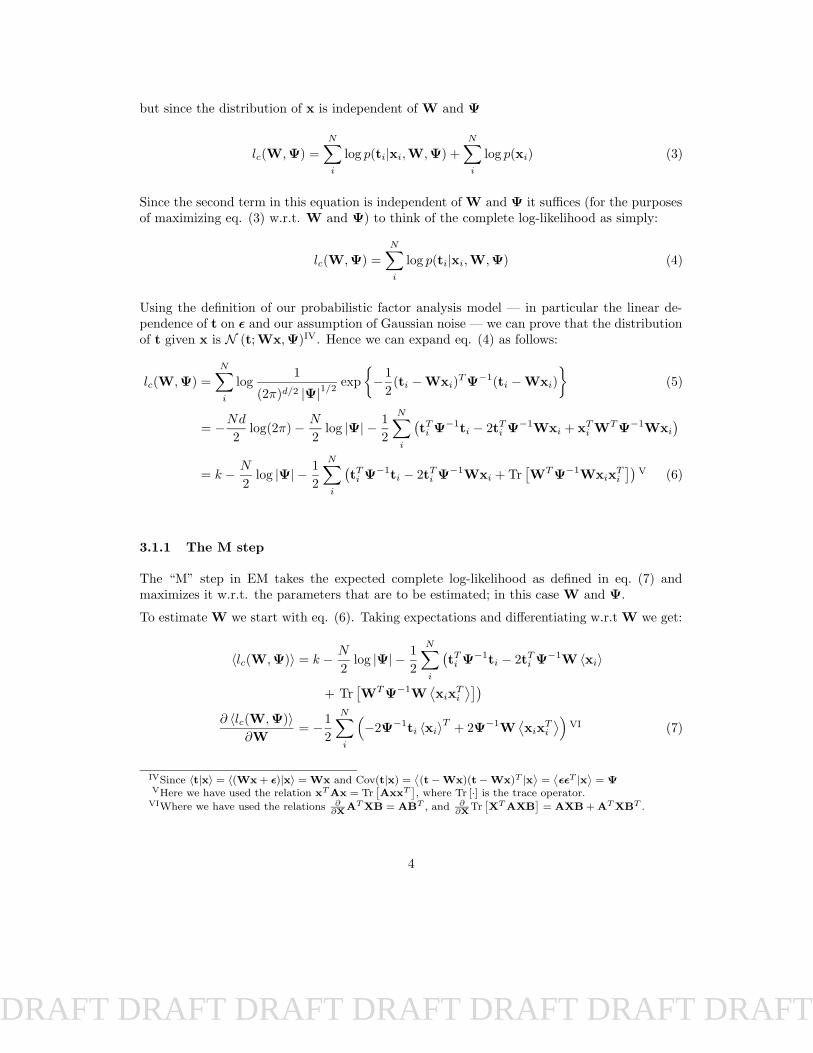
Figure 2: Graphical model for inferring the underlying latent variable dimensionality using agaussian approximation.

of the dimensionality q of the underlying distribution. In doing so one runs the risk of selectingtoo high a value of q and overfitting the data by explaining noise, or of selecting too low avalue and over generalizing, resulting in not capturing the true data complexity.

Each column of the W matrix represents one dimension of the underlying latent variable space.What is required is a way for us to determine how many columns of W are actually relevantbased on the data that is presented to us. In some sense, the number of columns of W is ameasure of our factor analysis model complexity — the larger the value of q, the greater themodel complexity since it can explain (or generate) a larger family of data sets.

In order to determine the most appropriate latent variable dimensionality, we start with themaximum possible value of q = d − 1, but place a prior distribution over each of the d − 1columns of W parameterized by a precision parameter α which functions as an inverse sphericalcovariance for each column. Hence we can write the distribution of W as follows:

p(W|α) =d−1∏

i

(αi2π

)d/2exp

(−αi

2wTi wi

)(17)

This change in model structure is reflected in our updated graphical model as shown in figure 2.Here we see a new node α being added as a parent to W. Also the W node has been changedfrom a rectangular node to a circle, reflecting the fact that we now have a prior distributionover W and that we can estimate a posterior distribution for this variable using Bayesiananalysis rather than merely compute a maximum likelihood estimate of its value. Using Bayesrule we have:

p(W|D,α) ∝ p(D|W)p(W|α) (18)

and hence

log p(W|D,α) = const+ log p(D|W) + log p(W|α) (19)

Since we have a distribution over W, in practice we would like to find the maximum a posteriorivalue WMP of this distribution, which means finding the value of W which maximizes eq. (19).

7


Since we know that the complete log-likelihood lc is a lower bound to the true data log-likelihood, we can substitute lc for log p(D|W) and try to maximize this new equation.

log p(W|D,α) = const+ lc(W,Ψ) + log p(W|α) (20)

which using eq. (17) and discarding terms that are independent of W and Ψ gives us:

log p(W|D,α) = lc(W,Ψ)− 1

2

d−1∑

i

αiwTi wi (21)

= lc(W,Ψ)− 1

2Tr[WAWT

](22)

Which is simply the complete log-likelihood with a regularization term that penalizes solutionsof W with higher intrinsic dimensionality. EM still applies within this framework and we candifferentiate the expectation of this regularized likelihood to derive the update equations forW and Ψ. Substituting from eq. (6) and taking expectations we get:

〈log p(W|D,α)〉 = −1

2

N∑

i

(tTi Ψ−1ti − 2tTi Ψ−1W 〈xi〉+ Tr

[WTΨ−1W

⟨xix

Ti

⟩])

− 1

2Tr[WAWT

]− N

2log |Ψ|+ k (23)

Maximizing w.r.t. W we get:

∂ 〈log p(W|D,α)〉∂W

= −1

2

N∑

i

(−2Ψ−1ti 〈xi〉T + 2Ψ−1W

⟨xix

Ti

⟩)−WA = 0VIII (24)

Hence

WN∑

i

⟨xix

Ti

⟩+ ΨWA =

N∑

i

ti 〈xi〉T (25)

or equivalently

WS + ΨWA = m (26)

Where we define S ≡∑Ni

⟨xix

Ti

⟩and m ≡∑N

i ti 〈xi〉T

Since Ψ is a diagonal matrix, we can obtain a closed form solution for each row of W individ-ually. For the kth row:

wk = mk(S + pkA)−1 (27)

Where wk and mi are the kth rows of W and m respectively, pk is the kth diagonal elementof Ψ, and 1 ≤ k ≤ d.

VIIIWhere we have used the relation ∂∂X

Tr[XAXT

]= X

(A + AT

)

8


4.1 Estimation of α

From the graphical model in figure 2 we see that in order to compute the likelihood of the datagiven the hyperparameters α we must integrate over the distribution of W

p(D|α) =

∫p(D|W,α)p(W|α)dW

=

∫p(D|W)p(W|α)dW (28)

Now since we assume that our observed data is Independently Identically Distributed (IID) wecan write:

p(D|W) =

N∏

i

p(t|W) (29)

=

[1

(2π)d/2 |C|1/2

]Nexp

{−1

2

N∑

i

tTi C−1ti

}(30)

=

[1

(2π)d/2

]Nexp

{−1

2

N∑

i

(tTi C−1ti + log |C|

)}

(31)

Where C = WWT + Ψ is the covariance matrix of the observed dataIX. Hence using eq. (17)for p(D|W) along with eq. (31) in eq. (28) we get:

p(D|α) ∝[d−1∏

i

(αi2π

)d/2]∫

exp

{−1

2

N∑

i


)− 1

2

d−1∑

i

αiwTi wi

}dW (32)

=

[d−1∏

i

(αi2π

)d/2]∫

exp {−S(W)} dW (33)

Where we define

S(W) ≡ 1

2

N∑

i


)+

1

2

d−1∑

i

αiwTi wi (34)

IXThis is trivially shown:

〈t〉 = 〈Wx + ε〉 = W 〈x〉+ 〈ε〉 = 0

Cov(t) =⟨ttT

⟩=⟨

(Wx + ε)(Wx + ε)T⟩

= W⟨xxT

⟩WT + W

⟨xεT

⟩+⟨εxT

⟩WT +

⟨εεT

⟩

= WWT + 0 + 0 + Ψ

= WWT + Ψ ≡ C

9


Approximate S(W) with a second-order Taylor series expansion around the extremal pointWMP . Since the first order derivative at an extremal is zero, our expansion does not containa linear term.

S(W) ≈ S(WMP ) +1

2(W −WMP )TH(W −WMP ) (35)

Where H is the d(d − 1) × d(d − 1) Hessian matrix of S(·) evaluated at WMP . Using thisapproximation to S(W) we can now evaluate the integral

∫exp {−S(W)} dW ≈

∫exp

{−S(WMP )− 1

2(W −WMP )TH(W −WMP )

}dW

= exp {−S(WMP )}∫

exp

{−1

2(W −WMP )TH(W −WMP )

}dW

= exp {−S(WMP )} (2π)d(d−1)/2∣∣H−1

∣∣1/2 (36)

Where the value of the integral is now simply the normalizing constant for a gaussian distri-bution in W with covariance H−1. Substituting this result back into eq. (33) we get:

p(D|α) ∝[d−1∏

i

(αi2π

)d/2]

exp {−S(WMP )} (2π)d(d−1)/2∣∣H−1

∣∣1/2 (37)

or equivalently

log p(D|α) = const+d

2

d−1∑

i

logαi − S(WMP )− 1

2log |H| (38)

Differentiating w.r.t. αk we get:

∂ log p(D|α)

∂αk=

∂

∂αk

[d−1∑

i

d

2logαi

]− ∂

∂αkS(WMP )− 1

2

∂

∂αklog |H| (39)

Now using eq. (34) we have:∂

∂αkS(WMP ) =

1

2‖wMP

k ‖2 (40)

In order to compute the partial derivative of H w.r.t. αk let us express S(W) as follows:

S(W) = EW + Eα (41)

where we define EW ≡ 12

∑Ni


)and Eα ≡ 1

2

∑d−1i αiw

Ti wi. Hence we can

write the Hessian of S(W) as:H = ∇∇EW +∇∇Eα (42)

10


Now if we assume that W is structured such that each column is lined up to form a largevector of dimensionality d(d− 1), then we can write:

∇∇Eα =

α1Id 0 . . . . . . . . . .0 α2Id 0 . . . . . . .

. . . . . . . . . . . . . . . . . . . . . . . .

. . . . . . . . . . . 0 αd−1Id

(43)

Hence we can view ∇∇Eα as a block diagonal matrix, where each d × d block along thediagonal is a unit matrix scaled by a corresponding αi. Let λij be the jth eigenvalue of the ith

diagonal submatrix of ∇∇EW. Since the determinant of a matrix is equal to the product ofit’s eigenvaluesX, we can write:

∂ log |H|∂αk

=∂

∂αklog

d−1∏

i

d∏

j

(λij + αi)

=∂

∂αk

d−1∑

i

d∑

j

log(λij + αi)

=

d∑

j

1

λkj + αk

= Trk[H−1

](44)

Hence substituting from eqs. (40) and (44) back into eq. (39) gives us:

∂ log p(D|α)

∂αk=

d

2αk− 1

2‖wMP

k ‖2 − 1

2Trk

[H−1

]= 0 (45)

Solving for αk we arrive at the update equation:

αk =d

‖wMPk ‖2 + Trk [H−1]

(46)

If we make the assumption that the parameter W is well determined, then its posterior distri-bution will be sharply peaked, which means H will have large eigenvalues. This also impliesthat Trk

[H−1

]will be very small. Under this assumption, eq. (46) for αk reduces to:

αk =d

‖wMPk ‖2 (47)

This avoids costly computation and manipulation of the d(d− 1)× d(d− 1) Hessian matrix.

XThis can be proved trivially; we can decompose a matrix A into the product A = VDVT , where V is amatrix of eigenvectors, and D is a diagonal matrix of the corresponding eigenvalues λi. Since V is orthonormal(implying |V| = 1), we have |A| = |D| = ∏

i λi.

11


When doing the Taylor series expansion of S(W) in eq. (35) we assumed that our currentestimate of W is a (possibly local) extremum. This assumption was important since it allowedus to eliminate the linear term in the expansion and retain only the quadratic term, makingit a Gaussian approximation to the posterior distribution. Algorithmically this means that weshould perform our EM iterations to update W (and Ψ) given a fixed current estimate of thevalue of α. When these iterations converge then we know that we have reached an extremum,and we can use the current value of W to re-estimate α. Thus our algorithm performs the EMupdates with an outer loop that periodically re-estimates the value of α.

In general since EM operates in a maximum likelihood framework, it will favour higher dimen-sionalities of W since this will always result in an increase in the likelihood. However, by usingthe α as a precision parameter on each of the columns of W we create a penalized likelihoodwhich seeks to limit the model complexity (dimensionality). By formulating the problem thisway EM results in a compromise between maximizing the dimensionality to increase likelihood,and reducing the penalizing term (which increases with the dimensionality).

5 Inferring Underlying Dimensionality — Variational Ap-proximation

If anything, the previous section should give us a hint that as the model complexity increases,integrating over the model parameter distributions becomes increasingly more complex, andindeed eventually analytically intractable. In the previous section itself, we fit a Gaussiandistribution to the posterior distribution of W in order to be able to integrate over it. We couldalso adopt a sampling approach and use Monte Carlo methods to give us an approximation tothe true distribution. In general however, sampling approaches tend to be expensive; both interms of computation and in terms of storage since the probability distributions are effectivelyrepresented by a collection of samples.

In this section we will explore Variational Methods as another method of approximating theposterior distributions of model parameters. Variational methods have long been used instatistical physics, and have recently been getting significant attention from the statisticallearning community. In essence, variational methods allow us to create a bound on the functionof interest (in our case the log-evidence for the observed data). Subsequent analysis then workstowards minimizing the difference between the bound and the true function.

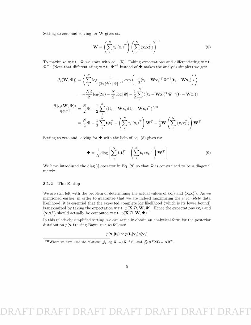
Let us begin by augmenting our factor analysis model to place a probability distribution overall parameters whose cardinality scales with model complexity. As shown in fig. 3, we havenow placed a probability distribution over the α precision parameters as well. Since theseparameters cannot be negative (being inverse covariances for each column vector of W), wecannot place a Gaussian distribution over them. Instead we place a Gamma prior over the αvariables:

p(α) =

q∏

i

G (αi; aα, bα) XI (48)

12


t i

xiα

W

aα

bα

Ψ

µ

N

Figure 3: Graphical model for learning a factor analyzer with automatic dimensionality esti-mation

Let us now look at the log probability of the observed data D (also known as the evidence).This can be obtained by marginalizing over all the model parameters and hidden variables asfollows:

log p(D) = log

∫p(D,X,W,α)dXdWdα (49)

Using Jensen’s inequality, we can lower-bound this quantity as follows:

log p(D) ≥∫Q(X,W,α) log

p(D,X,W,α)

Q(X,W,α)dXdWdα = F(Q) (50)

for any arbitrary distribution Q(X,W,α).

Maximizing the functional F(Q) is equivalent to minimizing the Kullback-Liebler divergencebetween Q and the true posterior distribution p(X,W,α|D)XII. There are two ways of assum-ing a functional form for Q. One is to assume a parameterized version of the distribution whichsimplifies its analytical form at the expense of introducing extra “variational” parameters thatmust be optimized. Another approach is to assume a factorized form for the distribution. Thisis the approach we shall take here. We assume the factorization:

Q(X,W,α) = Q(X)Q(W)Q(α) (51)

XIWe use the notation G (x; a, b) to denote the Gamma distribution which is mathematically defined as:

G (x; a, b) =ba

Γ(a)xa−1 exp(−bx)

XIIThis can be easily proved as follows:

log p(D) =

∫Q(θ) log p(D)dθ =

∫Q(θ) log

p(D, θ)

p(θ|D)dθ =

∫Q(θ) log

p(D, θ)

Q(θ)dθ +

∫Q(θ) log

Q(θ)

p(θ|D)dθ

=

∫Q(θ) log

p(D, θ)

Q(θ)dθ +KL {Q(θ)‖p(θ|D)}

13


Using the calculus of variations we can prove (see appendix B) that the solution for each ofthe individual Q distributions that maximizes the functional F(Q) is of the form:

Qi(θi) =exp 〈log p(D,θ)〉Qk 6=i∫

exp 〈log p(D,θ)〉Qk 6=i dθi(52)

or equivalently

logQi(θi) = 〈log p(D,θ)〉Qk 6=i + const (53)

Where θ = {X,W,α} and 〈·〉Qk 6=i denotes expectation taken with respect to every distribution

other than Qi(θi).

Let us first determine the expression for p(D,θ). The graphical model makes this easy toexpress:

p(D,θ) =

[N∏

i

p(ti|xi,W)p(xi)

]p(W|α)p(α) (54)

and hence

log p(D,θ) =

N∑

i

log p(ti|xi,W) +

N∑

i

log p(xi) + log p(W|α) + log p(α) (55)

= −N2

log |Ψ| − 1

2

N∑

i

(ti −Wxi)TΨ−1(ti −Wxi)

− 1

2

N∑

i

xTi xi

+d

2

q∑

i

logαi −1

2

q∑

i

αiwTi wi

+

q∑

i

(aα − 1) logαi −q∑

i

bααi + const (56)

5.1 Estimation of Q(α)

To obtain an expression for Q(α) using eq. (53), we take expectations of eq. (56) w.r.t. thedistribution Q(W)Q(X). All terms not involving α can conveniently be clubbed into a constterm at the end of the equation, and contribute to the normalizing constants in the distribution

14


of α.

〈log p(D,θ)〉Q(W)Q(X) =d

2

q∑

i

logαi −1

2

q∑

i

αi⟨‖wi‖2

⟩

+

q∑

i

(aα − 1) logαi −q∑

i

bααi + const

=

q∑

i

(aα +d

2− 1) logαi −

q∑

i

(bα +

⟨‖wi‖2

⟩

2

)αi + const (57)

Since we havelogQ(α) = 〈log p(D,θ)〉Q(W)Q(X) + const (58)

we can infer that Q(α) is of the form:

Q(α) =

q∏

i

Q(αi) (59)

=

q∏

i

G(αi; aα, b

(i)α

)(60)

where

aα = aα +d

2(61)

b(i)α = bα +

⟨‖wi‖2

⟩

2(62)

5.2 Estimation of Q(W)

In order to estimate Q(W) we start with eq. (56) and retain only the terms that contain W

log p(D,θ) = −1

2

N∑

i

(ti −Wxi)TΨ−1(ti −Wxi)−

1

2

q∑

i

αiwTi wi + const (63)

This equation can be rewritten as follows:

log p(D,θ) = −1

2

N∑

i

d∑

k

pk(tik −wT

k xi)2 − 1

2

d∑

k

wTk Awk + const

= −1

2

N∑

i

d∑

k

pk(t2ik − 2tikw

Tk xi + wT

k xixTi wk

)− 1

2

d∑

k

wTk Awk + const

= −1

2

d∑

k

pk

[N∑

i

t2ik − 2wTk

(N∑

i

tikxi

)+ wT

k

(N∑

i

xixTi +

1

pkA

)wk

]+ const

(64)

15


where wk is a column vector corresponding to the kth row of W, A = diag [α], and pk is thekth diagonal element of Ψ−1. Taking expectations according to Q(X)Q(α) we get:

〈log p(D,θ)〉Q(X)Q(α) = −1

2

d∑

k

pk

[N∑

i

t2ik − 2wTk

(N∑

i

tik 〈xi〉)

+wTk

(N∑

i

⟨xix

Ti

⟩+

1

pk〈A〉

)wk

]+ const (65)

Since this is a quadratic in wk and since we know that

logQ(W) = 〈log p(D,θ)〉Q(X)Q(α) + const (66)

we can infer that Q(W) is of the form:

Q(W) =d∏

k

Q(wk) (67)

=

d∏

k

N(wk; m(k)

w ,Σ(k)w

)(68)

where

Σ(k)w =

(pk

N∑

i

⟨xix

Ti

⟩+ 〈A〉

)−1

(69)

m(k)w = pkΣ

(k)w

(N∑

i

tik 〈xi〉)

(70)

5.3 Estimation of Q(X)

Take expectations of eq. (56) w.r.t. Q(W)Q(α) and (for simplicity) retain only the terms thatcontain xi.

〈log p(D,θ)〉Q(W)Q(α) = −1

2

N∑

i

(tTi Ψ−1ti − 2xTi

⟨WT

⟩Ψ−1ti + xTi

⟨WTΨ−1W

⟩xi)

− 1

2

N∑

i

xTi xi (71)

= −1

2

N∑

i

(tTi Ψ−1ti − 2xTi

⟨WT

⟩Ψ−1ti + xTi

(I +

⟨WTΨ−1W

⟩)xi)

(72)

16


Since we havelogQ(X) = 〈log p(D,θ)〉Q(W)Q(α) + const (73)

we can infer that Q(X) is of the form:

Q(X) =N∏

i

Q(xi) (74)

=N∏

i

N(xi; m

(i)x ,Σx

)(75)

where

Σx =(I +

⟨WTΨ−1W

⟩)−1(76)

m(i)x = Σx

⟨WT

⟩Ψ−1ti (77)

5.4 Calculation of the required expectations

Most of the moments required in the update equations can be obtained directly given the formof the distributions. For a Gaussian distribution for example, the expectation is simply themean of the distribution. A slightly non-trivial expectation is

⟨WTΨ−1W

⟩which occurs in

eq. (76). To compute this expectation we use the fact that Ψ−1 is a diagonal matrix as follows:

⟨WTΨ−1W

⟩=

⟨d∑

k

1

pkwkw

Tk

⟩

=

d∑

k

1

pk

⟨wkw

Tk

⟩(78)

Where wk is the kth row of W, and pk is the kth diagonal element of Ψ. Since we have shownthat the distribution of each row of W is Gaussian with covariances and means as shown ineqs. (69) and (70) we can compute the required second order moments trivially.

5.5 Maximization equation for Ψ

The noise covariance matrix is estimated using the standard EM algorithm. Differentiatingthe expectation of Eq. (56) w.r.t. Ψ−1, we get:

Ψ =1

N

N∑

i

⟨(ti −Wxi)(ti −Wxi)

T⟩

(79)

=1

N

[N∑

i

titTi − 2 〈W〉

( N∑

i

〈xi〉 tTi)

+N∑

i

⟨Wxix

Ti WT

⟩]

(80)

17


Our only difficulty is in computing the term∑Ni

⟨Wxix

Ti WT

⟩. We can work our way around

this by noting that only the diagonal terms of Ψ are of interest. For this term, the kth diagonalelement can be written as follows:

diagk

[N∑

i

⟨Wxix

Ti WT

⟩]

=N∑

i

⟨wTk xix

Ti wk

⟩(81)

= Tr

[⟨wkw

Tk

⟩ N∑

i

〈xixi〉]

(82)

= Tr

[Σk

w

(NΣx +

N∑

i

〈xi〉〈xi〉T)]

+ 〈wk〉(NΣx +

N∑

i

〈xi〉〈xi〉T)〈wk〉T

(83)

5.6 Measuring success: High F(Q) or low KL {Q(θ)‖p(θ|D)}?

It must be pointed out that the variational framework is not inherently an approximation initself. Free-form maximization of the functional F(Q) results in the solution that effectivelyreduces KL {Q(θ)‖p(θ|D)} to zero. However, it must be pointed out that we introduce theapproximation, when we restrict Q to have a factorized form. Given this restriction, a highvalue of F(Q) does not necessarily mean that we have obtained a good approximation to theform of the posterior distribution. Conversely, a low value for the KL divergence between Qand the true posterior does not imply that we will have the tightest bound on the log-evidenceof the data.

Which quantity then, is an appropriate measure of success? If we are doing Bayesian inference,then we are most likely interested in obtaining an approximation to the posterior that is asgood as possible. In this case, the KL divergence is the true measure of how well we haveinferred our model parameters from the data. If however, we are doing model comparison,then we would probably be more interested in achieving the tightest possible bound on thelog-evidence of the data under each of the models we are comparing so that we can accuratelyjudge the suitability of each model to the dataset at hand.

6 Modelling Nonlinear Manifolds — Mixture Models

Factor analysis is a linear model. This very fact makes it unsuitable for modelling non-linearmanifolds. By using multiple factor analyzers however, we can create a soft partition of thedata space such that each factor analyzer models a locally linear region of the manifold.

Using a mixture of factor analysis requires considerable extension to our graphical model aswe can see in fig. 4. Each individual factor analyzer must automatically position itself withinthe input space (by adjusting its mean vector), and determine its appropriate factor loadingmatrix. In addition, each factor analyzer must also determine its own dimensionality. These

18


Ψ

αm

µm

t i

xi

si

aα

bα

Wm

βm

u

π

M

N

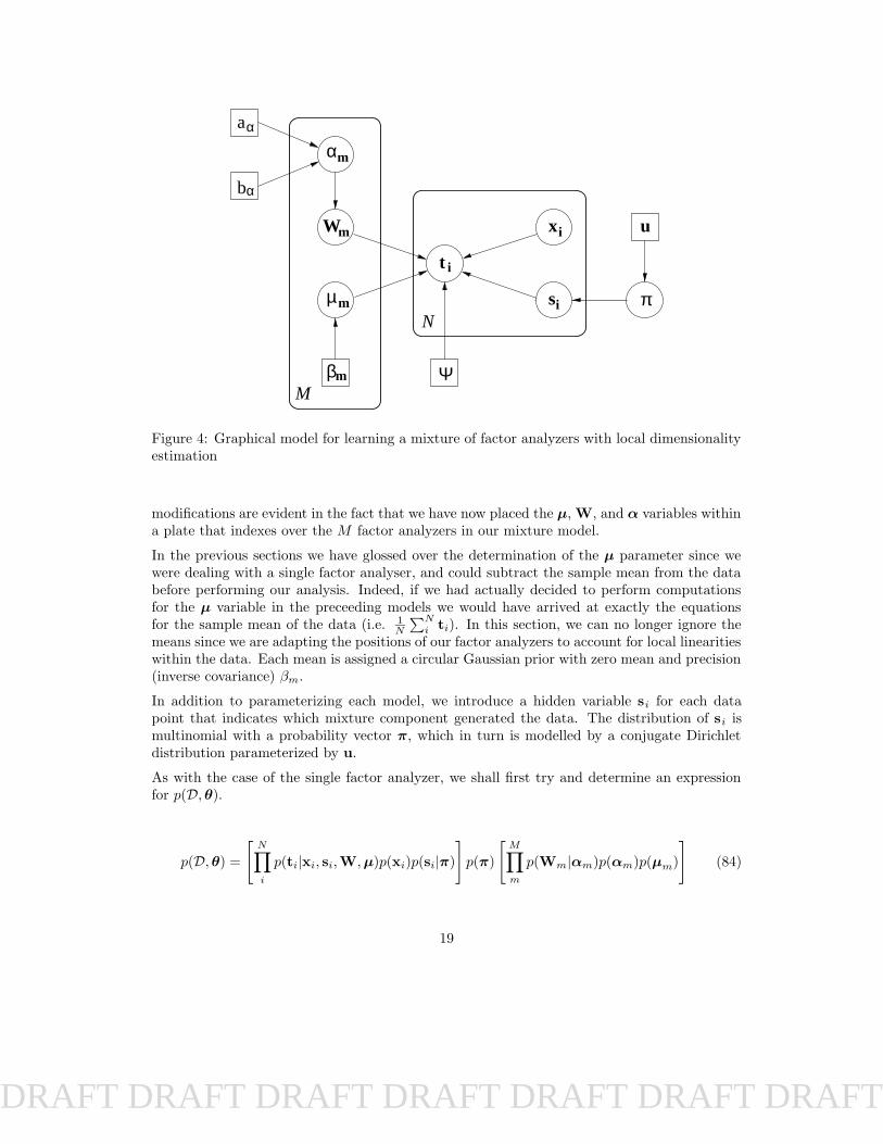
Figure 4: Graphical model for learning a mixture of factor analyzers with local dimensionalityestimation

modifications are evident in the fact that we have now placed the µ, W, and α variables withina plate that indexes over the M factor analyzers in our mixture model.

In the previous sections we have glossed over the determination of the µ parameter since wewere dealing with a single factor analyser, and could subtract the sample mean from the databefore performing our analysis. Indeed, if we had actually decided to perform computationsfor the µ variable in the preceeding models we would have arrived at exactly the equationsfor the sample mean of the data (i.e. 1

N

∑Ni ti). In this section, we can no longer ignore the

means since we are adapting the positions of our factor analyzers to account for local linearitieswithin the data. Each mean is assigned a circular Gaussian prior with zero mean and precision(inverse covariance) βm.

In addition to parameterizing each model, we introduce a hidden variable si for each datapoint that indicates which mixture component generated the data. The distribution of si ismultinomial with a probability vector π, which in turn is modelled by a conjugate Dirichletdistribution parameterized by u.

As with the case of the single factor analyzer, we shall first try and determine an expressionfor p(D,θ).

p(D,θ) =

[N∏

i

p(ti|xi, si,W,µ)p(xi)p(si|π)

]p(π)

[M∏

m

p(Wm|αm)p(αm)p(µm)

](84)

19


=

[N∏

i

M∏

m

[p(ti|xi, sim,Wm,µm)p(xi)p(sim|π)]sim

]p(π) (85)

·[M∏

m

p(Wm|αm)p(αm)p(µm)

](86)

And hence

log p(D,θ) =N∑

i

M∑

m

sim [log p(ti|xi, sim,Wm,µm) + log p(xi) + log p(sim|π)]

+ log p(π) +M∑

m

[log p(Wm|αm) + log p(αm) + log p(µm)]

(87)

= −1

2

N∑

i

M∑

m

sim(ti −Wmxi − µm)TΨ−1(ti −Wmxi − µm)

− 1

2

N∑

i

M∑

m

simxTi xi +N∑

i

M∑

m

sim logπm

+M∑

m

(um − 1) logπm

+M∑

m

q∑

i

d

2logαim −

1

2

M∑

m

q∑

i

αimwTimwim

+M∑

m

q∑

i

(aα − 1) logαim −M∑

m

q∑

i

bααim

− 1

2

M∑

m

βmµTmµm + const

(88)

We assume the factorization

Q(X,S,W,α,π,µ) = Q(X,S)Q(W)Q(α)Q(π)Q(µ)

= Q(X|S)Q(S)Q(W)Q(α)Q(π)Q(µ) (89)

6.1 Estimation of Q(π)

Taking expectations of eq. (88) w.r.t. all distributions except Q(π) and retaining only theterms containing π we get:

20


〈log p(D,θ)〉Qθ−{π} =N∑

i

M∑

m

〈sim〉 logπm +M∑

m

(um − 1) logπm + const (90)

=M∑

m

(um +

N∑

i

〈sim〉 − 1

)logπm + const (91)

We can infer:

Q(π) = D(π; u)XIII (92)

where

um = um +N∑

i

〈sim〉 (93)

6.2 Estimation of Q(α)

Taking expectations of eq. (88) w.r.t. all distributions except Q(α) and retaining only theterms containing α we get:

〈log p(D,θ)〉Qθ−{α} =M∑

m

q∑

i

d

2logαim −

1

2

M∑

m

q∑

i

αim⟨‖wim‖2

⟩

+M∑

m

q∑

i

(aα − 1) logαim −M∑

m

q∑

i

bααim + const (94)

=M∑

m

q∑

i

(aα +

d

2− 1

)logαim −

M∑

m

q∑

i

(bα +

⟨‖wim‖2

⟩

2

)αim + const

(95)

Q(α) =M∏

m

q∏

i

Q(αim) (96)

=

M∏

m

q∏

i

G(αim; aα, b

(im)α

)(97)

XIIIWe use the notation D (π; u) to denote the Dirichlet distribution which is mathematically defined as:

D (π; u) =Γ(∑M

m um)

∏Mm Γ(um)

M∏

m

πum−1m

21


where

aα = aα +d

2(98)

b(im)α = bα +

⟨‖wim‖2

⟩

2(99)

6.3 Estimation of Q(µ)

〈log p(D,θ)〉Qθ−{µ} = −1

2

N∑

i

M∑

m

〈sim〉⟨(ti −Wmxi − µm)TΨ−1(ti −Wmxi − µm)

⟩

− 1

2

M∑

m

βmµTmµm + const (100)

= −1

2

N∑

i

M∑

m

〈sim〉[µTmΨ−1µm − 2µTmΨ−1(ti − 〈Wm〉〈xi|m〉)

+(ti − 〈Wm〉〈xi|m〉)TΨ−1(ti − 〈Wm〉〈xi|m〉)]

(101)

− 1

2

M∑

m

βmµTmµm + const

= −1

2

M∑

m

[µTm

(βmI + Ψ−1

N∑

i

〈sim〉)µm

− 2µTmΨ−1N∑

i

〈sim〉 (ti − 〈Wm〉〈xi|m〉)

+N∑

i

〈sim〉 (ti − 〈Wm〉〈xi|m〉)TΨ−1(ti − 〈Wm〉〈xi|m〉)]

+ const

(102)

We can deduce

Q(µ) =

M∏

m

Q(µm)

=M∏

m

N(µm; mm

µ ,Σmµ

)(103)

22


where

Σmµ =

(βmI + Ψ−1

N∑

i

〈sim〉)−1

(104)

mmµ = Σm

µΨ−1N∑

i

〈sim〉 (ti − 〈Wm〉〈xi|m〉) (105)

6.4 Estimation of Q(W)

〈log p(D,θ)〉Qθ−{W} = −1

2

N∑

i

M∑

m


⟩

− 1

2

M∑

m

q∑

i

〈αim〉wTimwim + const

= −1

2

N∑

i

M∑

m

〈sim〉d∑

k

pk

⟨(tik −wT

mkxi − µmk)2⟩

(106)

− 1

2

M∑

m

d∑

k

wTmk 〈Am〉wmk + const

= −1

2

M∑

m

d∑

k

[pk

N∑

i

〈sim〉⟨(tik −wT

mkxi − µmk)2⟩

+ wTmk 〈Am〉wmk

]

+ const (107)

We can deduce

Q(W) =M∏

m

d∏

k

Q(wmk) (108)

=M∏

m

d∏

k

N(wmk; mm(k)

w ,Σm(k)w

)(109)

where

Σm(k)w =

(pk

N∑

i

〈sim〉⟨xix

Ti |m

⟩+ 〈Am〉

)−1

(110)

mm(k)w = pkΣ

m(k)w

(N∑

i

〈sim〉〈xi|m〉 (tik − 〈µmk〉))

(111)

23


6.5 Estimation of Q(X|S)

Since the distribution of X is conditioned on S we must not take expectations w.r.t. Q(S).

〈log p(D,θ)〉Qθ−{X,S} = −1

2

N∑

i

M∑

m

sim⟨(ti −Wmxi − µm)TΨ−1(ti −Wmxi − µm)

⟩

− 1

2

N∑

i

M∑

m

simxTi xi + const

From which we can infer that

logQ(X|S) = log

N∏

i

Q(xi|si) (112)

= log

N∏

i

M∏

m

Q(xi|m)sim (113)

=

N∑

i

M∑

m

sim logQ(xi|m) (114)

where

Q(xi|m) = N(xi; m

m(i)x ,Σm

x

)(115)

and

Σmx =

(I +

⟨WT

mΨ−1Wm

⟩)−1(116)

mm(i)x = Σm

x 〈Wm〉T Ψ−1(ti − 〈µm〉) (117)

6.6 Estimation of Q(S)

Since the distribution Q(X|S) is conditioned on S we can derive (see appendix B.1):

logQ(S) = 〈log p(D,θ)〉Qθ−{S} + entropy {Q(X|S)}+ const (118)

Now we have

24


〈log p(D,θ)〉Qθ−{S} = −1

2

N∑

i

M∑

m

sim⟨(ti −Wmxi − µm)TΨ−1(ti −Wmxi − µm)

⟩

− 1

2

N∑

i

M∑

m

sim⟨xTi xi|m

⟩+

N∑

i

M∑

m

sim 〈logπm〉+ const (119)

also

entropy {Q(X|S)} = −∫Q(X|S) logQ(X|S)dX (120)

= −∫Q(X|S) log

N∏

i

M∏

m

Q(xi|m)simdX (121)

= −∫Q(X|S)

N∑

i

M∑

m

sim logQ(xi|m)dX (122)

Given that the posterior distributions of the X variables are independent Gaussian (see eqs.(114) and (115)) we can write:

entropy {Q(X|S)} = −N∑

i

M∑

m

sim

∫Q(xi|m) logQ(xi|m)dxi (123)

= −N∑

i

M∑

m

simentropy {Q(xi|m)} (124)

=1

2

N∑

i

M∑

m

sim log |Σmx |+ const (125)

From eqs. (118), (119) and (125), we can infer:

Q(S) =N∏

i

M∏

m

Q(sim = 1)sim (126)

where

logQ(sim = 1) = −1

2

{tTi Ψ−1ti − 2tTi Ψ−1 〈Wm〉〈xi|m〉 − 2tTi Ψ−1 〈µm〉

+ 2⟨µTm⟩Ψ−1 〈Wm〉〈xi|m〉+ Tr

[⟨WT

mΨ−1Wm

⟩ ⟨xix

Ti |m

⟩]

+ Tr[Ψ−1

⟨µmµ

Tm

⟩]}+ 〈logπm〉 −

1

2

⟨xTi xi|m

⟩+

1

2log |Σm

x |+ const

(127)

25


The constant term in the above equation can be determined by normalizing. We have encoun-tered all the above sufficient statistics before except for 〈logπm〉. Given that the distributionQ(π) is Dirichlet, we can use the result:

〈logπm〉 = ψ (um)− ψ

M∑

j

uj

(128)

where ψ (·) is the Digamma function defined as follows:

ψ (x) =∂

∂xlog Γ (x) (129)

6.7 Maximization equation for Ψ

The noise covariance matrix is estimated using the standard EM algorithm. Differentiatingthe expectation of Eq. (88) w.r.t. Ψ−1, we get:

Ψ =1

N

N∑

i

M∑

m

〈sim〉⟨(ti −Wmxi − µm)(ti −Wmxi − µm)T

⟩(130)

=1

N

[N∑

i

titTi − 2

M∑

m

( N∑

i

〈sim〉 ti)〈µm〉T +

M∑

m

( N∑

i

〈sim〉)(

Σmµ + 〈µm〉〈µm〉T

)

− 2M∑

m

〈Wm〉( N∑

i

〈sim〉xi(ti − 〈µm〉

)T)

+N∑

i

M∑

m

〈sim〉⟨Wmxix

Ti WT

m

⟩]

(131)

Our only difficulty is in computing the term∑Ni

∑Mm 〈sim〉

⟨Wmxix

Ti WT

m

⟩. We can work our

way around this by noting that only the diagonal terms of Ψ are of interest. For this term,the kth diagonal element can be written as follows:

diagk

[ N∑

i

M∑

m

〈sim〉⟨Wmxix

Ti WT

m

⟩]=

N∑

i

M∑

m

〈sim〉⟨wTmkxix

Ti wmk

⟩(132)

=

M∑

m

Tr

[⟨wmkw

Tmk

⟩ N∑

i

〈sim〉〈xixi|m〉]

(133)

Typically the matrix Ψ in Eq. (131) is diagonalized after it is computed, but by realizing thatonly its diagonal terms are required, we may be able to write the expression simply for the kth

26


diagonal term in a manner which is numerically much more efficient.

diagk[Ψ] =1

N

N∑

i

M∑

m


mkxi − µmk)2⟩

(134)

=1

N

[N∑

i

t2ik − 2

M∑

m

( N∑

i

〈sim〉 tik)〈µmk〉+

M∑

m

( N∑

i

〈sim〉)(

Σmµ (k, k) + 〈µmk〉2

)

− 2

M∑

m

〈wmk〉T( N∑

i

〈sim〉xi(tik − 〈µmk〉

))

+

M∑

m

Tr

[⟨wmkw

Tmk

⟩ N∑

i

〈sim〉〈xixi|m〉]]

(135)

6.8 Functional monitoring

From our definition of the functional F(Q) in Eq. (50), we can write:

F(Q) =

∫Q(θ) log

p(D,θ)

Q(θ)dθ (136)

= 〈log p(D,θ)〉Q(θ) + Entropy[Q(θ)] (137)

From Eq. (87) we have:

〈log p(D,θ)〉 =N∑

i

M∑

m

〈sim〉[〈log p(ti|xi, sim,Wm,µm)〉+ 〈log p(xi)〉+ 〈log p(sim|π)〉

]

+ 〈log p(π)〉+M∑

m

[〈log p(Wm|αm)〉+ 〈log p(αm)〉+ 〈log p(µm)〉

]

(138)

Consider each of the above terms individually:

N∑

i

M∑

m

〈sim〉〈log p(ti|xi, sim,Wm,µm)〉 (139)

= −N2

log |Ψ| − 1

2

N∑

i

M∑

m


⟩+ const

(140)

= −N2

log |Ψ| − 1

2

d∑

k

1

diagk[Ψ]

N∑

i

M∑

m


mkxi − µmk)2⟩

︸︷︷︸=Ndiagk[Ψ] (see Eq. (134))

+const (141)

27


= −N2

log |Ψ| − 1

2Nd+ const (142)

= −N2

log |Ψ|+ const (143)

N∑

i

M∑

m

〈sim〉〈log p(xi)〉 = −1

2

N∑

i

M∑

m

〈sim〉⟨xTi xi|m

⟩+ const (144)

= −1

2

N∑

i

M∑

m

〈sim〉Tr[⟨

xixTi |m

⟩]+ const (145)

= −1

2

M∑

m

( N∑

i

〈sim〉)

Tr [Σmx ]− 1

2

M∑

m

N∑

i

〈sim〉〈xi|m〉T 〈xi|m〉+ const

(146)

N∑

i

M∑

m

〈sim〉〈log p(sim|π)〉 =N∑

i

M∑

m

〈sim〉〈log πm〉 (147)

=N∑

i

M∑

m

〈sim〉(ψ(um)− ψ(u0)

)(148)

=M∑

m

( N∑

i

〈sim〉)ψ(um)−Nψ(u0) (149)

〈log p(π)〉 = log Γ(u0)−M∑

m

log Γ(um) +M∑

m

(um − 1) 〈log πm〉 (150)

= log Γ(u0)−M∑

m

log Γ(um) +

M∑

m

(um − 1)(ψ(um)− ψ(u0)

)(151)

= log Γ(u0)−M∑

m

log Γ(um) +M∑

m

(um − 1)ψ(um)− ψ(u0)M∑

m

(um − 1) (152)

M∑

m

〈log p(Wm|αm)〉 =d

2

M∑

m

q∑

i

〈logαmi〉 −1

2

M∑

m

q∑

i

〈αmi〉⟨wTmiwmi

⟩(153)

=d

2

M∑

m

q∑

i

(ψ(aα)− log b(mi)α

)− 1

2

M∑

m

d∑

k

⟨wTmkAmwmk

⟩(154)

=d

2

M∑

m

q∑

i


)− 1

2

M∑

m

d∑

k

Tr[⟨

wmkwTmk

⟩〈Am〉

](155)

28


=d

2

M∑

m

q∑

i


)− 1

2

M∑

m

( d∑

k

Tr[Σm(k)

w 〈Am〉])

− 1

2

M∑

m

d∑

k

〈wmk〉T 〈Am〉〈wmk〉(156)

M∑

m

〈log p(αm)〉 =M∑

m

q∑

i

(aα log bα − log Γ(aα)

)+ (aα − 1)

M∑

m

q∑

i

〈logαmi〉

− bαM∑

m

q∑

i

〈αmi〉(157)

= Mq(aα log bα − log Γ(aα)

)+ (aα − 1)

M∑

m

q∑

i


)

− bαM∑

m

q∑

i

〈αmi〉(158)

M∑

m

〈log p(µm)〉 =d

2

M∑

m

log βm −1

2

M∑

m

βm⟨µTmµm

⟩(159)

=d

2

M∑

m

log βm −1

2

M∑

m

βm

(Tr[Σmµ

]+ 〈µm〉T 〈µm〉

)(160)

We can compute the entropiesXIVof the various distributions as follows:

Entropy[Q(µ)] =M∑

m

Entropy[Q(µm)] (161)

=1

2

M∑

m

log((2πe)d

∣∣Σmµ

∣∣) (162)

=1

2

M∑

m

log∣∣Σmµ

∣∣+ const (163)

XIVEntropies of some standard distributions:

Entropy [N (x;µ,Σ)] =1

2log(

(2πe)d |Σ|)

Entropy [G (x; a, b)] = log Γ(a)− (a− 1)ψ(a)− log b+ a

Entropy [D (x; u)] = − log Γ(u0) +M∑

m

log Γ(um)−M∑

m

(um − 1)ψ(um) + ψ(u0)M∑

m

(um − 1)

29


Entropy[Q(W)] =M∑

m

d∑

k

Entropy[Q(wmk)] (164)

=1

2

M∑

m

d∑

k

log∣∣Σm(k)

w

∣∣+ const (165)

Entropy[Q(X,S)] = −∫Q(X|S)Q(S)

(logQ(X|S) + logQ(S)

)dXdS (166)

= −∫Q(X|S)Q(S) logQ(X|S)dXdS−

∫Q(X|S)Q(S) logQ(S)dXdS

(167)

= 〈Entropy[Q(X|S)]〉Q(S) + Entropy[Q(S)] (168)

which from Eq. (125) gives us:

=1

2

N∑

i

M∑

m

〈sim〉 log |Σmx | −

N∑

i

M∑

m

〈sim〉 log 〈sim〉 (169)

=1

2

M∑

m

( N∑

i

〈sim〉)

log |Σmx | −

N∑

i

M∑

m

〈sim〉 log 〈sim〉 (170)

Entropy[Q(α)] =M∑

m

q∑

i

Entropy[Q(α)] (171)

=M∑

m

q∑

i

log Γ(aα)− (aα − 1)ψ(aα)− log b(mi)α + aα (172)

= Mq(

log Γ(aα)− (aα − 1)ψ(aα) + aα

)−

M∑

m

q∑

i

log b(mi)α (173)

Entropy[Q(π)] = − log Γ(u0) +M∑

m

log Γ(um)−M∑

m

(um − 1)ψ(um) + ψ(u0)M∑

m

(um − 1)

(174)

30


6.8.1 Functional contribution of each model

In order to assess when a model needs to be split, we need to estimate the contribution of eachmodel to the overall functional. The functional is written as follows:

F(Q) =

∫dθQ(θ) log

p(D,θ)

Q(θ)(175)

=

∫dπQ(π) log

p(π)

Q(π)+

M∑

m

∫dµmQ(µm) log

p(µm)

Q(µm)

+M∑

m

∫dαmQ(αm)

[log

p(αm)

Q(α)+

∫dWmQ(Wm) log

p(Wm|αm)

Q(Wm)

]

+N∑

i

M∑

m

〈sim〉[∫

dπQ(π) logp(m|π)

Q(m)+

∫dxiQ(xi|m) log

p(xi)

Q(xi|m)

+

∫dµmQ(µm)

∫dWmQ(Wm)

∫dxiQ(xi|m)p(ti|xi,m,Wm,µm)

]

(176)

The last term in the expression (normalized by∑Ni 〈sim〉) is the contribution of each model

to the functional.

A Useful matrix algebra results

A.1 Matrix inversion theorem

The famous Sherman-Morrison-Woodbury theorem:

(A + XRY)−1 = A−1 −A−1X(R−1 + YA−1X)−1YA−1

A.2 Another useful result

A = WT (Ψ + WWT )−1

= WT[Ψ−1 −Ψ−1W(I + WTΨ−1W)−1WTΨ−1

]

=[I−WTΨ−1W(I + WTΨ−1W)−1

]WTΨ−1

=[I + (I + WTΨ−1W)−1 − (I + WTΨ−1W)(I + WTΨ−1W)−1

]WTΨ−1

= (I + WTΨ−1W)−1WTΨ−1

In a simliar fashion, we can also prove the more general result

WT (Ψ + WAWT )−1 = A−1(A−1 + WTΨ−1W)−1WTΨ−1

31


B Use of the factorial variational approximation

We lower bound the log evidence using Jensen’s inequality as follows:

log p(D) = log

∫p(D,θ)dθ (177)

= log

∫Q(θ)

p(D,θ)

Q(θ)dθ (178)

≥∫Q(θ) log

p(D,θ)

Q(θ)dθ = F(Q) (179)

Maximizing the lower bound implies maximizing the functional F(Q) over the space of proba-bility distributions Q(θ). If we assume that Q(θ) factors over the individual variables θi, thenwe can write Q(θ) =

∏iQi(θi). Let us consider a simple example in which θ = {θ1, θ2, θ3},

and Q(θ) = Q1(θ1)Q2(θ2)Q3(θ3). For the ease of notation, we shall use the symbol Qi todenote Qi(θi). Hence for our current example, our functional F(Q) is of the form:

F(Q) =

∫Q1Q2Q3 log

p(D,θ)

Q1Q2Q3dθ1dθ2dθ3 (180)

From the calculus of variations we know that maximizing F(Q) is actually a constrainedmaximization since we must ensure that

∫Q(θ)dθ = 1. This constraint can be incorporated

into the integrand by the use of Lagrange multipliers. To this end we define a new functionz(θ) as follows:

z(θ) =

∫ θ

−∞Q1(θ′1)Q2(θ′2)Q3(θ′3)dθ′1dθ

′2dθ′3 (181)

Giving us the differential constraint:

z −Q1Q2Q3 = 0 (182)

with the end point constraints being z(−∞) = 0 and z(∞) = 1. If we let g(Q1, Q2, Q3,θ)represent the integrand:

g(Q1, Q2, Q3,θ) = Q1Q2Q3 logp(D,θ)

Q1Q2Q3(183)

The we can incorporate the constraint into the integral by augmenting the integrand with thehelp of the Lagrange multiplier λ as follows:

ga(Q1, Q2, Q3,θ, z, λ) = Q1Q2Q3 logp(D,θ)

Q1Q2Q3+ λ(z −Q1Q2Q3) (184)

32


Maximizing the functional F(Q) w.r.t. each of the distributions Qi involves solving the Eulerequations:

∂ga∂Qi

− d

dθ

(∂ga

∂Qi

)= 0 (185)

∂ga∂z− d

dθ

(∂ga∂z

)= 0 (186)

Where Qi = dQi/dθ

Substituting from eq. (184) in eq. (186) we get:

dλ

dθ= 0 (187)

Which implies that λ is independent of θ = {θ1, θ2, θ3}. This is an important result that will beused in the following steps. Similarly substituting from eq. (184) in eq. (185) and performingthe differentiation with Qi = Q1 we get:

Q2Q3 [log p(D,θ)− logQ1 − logQ2Q3]−Q2Q3 − λQ2Q3 = 0 (188)

Integrating the above equation w.r.t. θ2 and θ3 we get:

〈log p(D,θ)〉Q2Q3− logQ1 −

∫Q2Q3 logQ2Q3dθ2dθ3 − 1− λ = 0 (189)

Solving for Q1 we get:

Q1 =exp 〈log p(D,θ)〉Q2Q3

exp(1 + λ+

∫Q2Q3 logQ2Q3dθ2dθ3

) (190)

From eq. (187) and the assumed factorization Q(θ) =∏iQi(θi) we know that the denominator

is independent of θ1 and can be treated as a normalizing constant. Hence in general wecan express the solution for the individual Qi that maximizes the functional F(Q) under theassumed factorization as:

Qi(θi) =exp 〈log p(D,θ)〉Qk 6=i∫

exp 〈log p(D,θ)〉Qk 6=i dθi(191)

B.1 Solution for partial factorization

Let us drop the assumption of complete factorization for now and examine how our solutionchanges when the factorization is partial. Suppose our current example had the partial fac-torization Q(θ) = Q12(θ1, θ2)Q3(θ3) = Q1(θ1|θ2)Q2(θ2)Q(θ3), then if we were trying to find

33


a solution for Q1 we would not be able to separate the logQ1 term out of the integral as wehave done in eq. (189), due to the fact that Q1 = Q1(θ1|θ2) and has a dependency on θ2. Ouronly way out of the problem is to infer the joint distribution Q12(θ1, θ2), and hope to be ableto factor the resulting distribution into Q1(θ1|θ2)Q2(θ2).

The final solution also changes if we were trying to maximize the functional w.r.t. Q2. Wewould proceed as if we assumed full factorization as before and arrive at the following equationwhich is analogous to eq. (189)

〈log p(D,θ)〉Q1Q3− logQ2 −

∫Q1Q3 logQ1Q3dθ1dθ3 − 1− λ = 0 (192)

In this situation however, we must keep in mind that Q1 is actually Q1(θ1|θ2) and hence has adependency on θ2. Now when we solve for Q2 we should take care to place all of the terms inthe equation that have a dependency on θ2 in the numerator. We then arrive at the equation:

Q2(θ2) ∝ exp

(〈log p(D,θ)〉Q1Q3

−∫Q1(θ1|θ2) logQ1(θ1|θ2)dθ1

)(193)

or equivalently

logQ2 = 〈log p(D,θ)〉Q1Q3+ entropy {Q1(θ1|θ2)}+ const (194)

C Computing 〈log x〉 and 〈log |X|〉 expectations from theGamma & Wishart distributions

(Thanks to Matt Beal for the hint about the derivation)

The Gamma distribution is frequently used as a conjugate prior to a precision (inverse variance)variable. The multivariate extension of this conjugate prior to precision (inverse covariance)matrices is the Wishart prior. These two distributions have the following form.

G (x; a, b) =ba

Γ(a)x(a−1) exp(−bx) (195)

W (X; ν,S) =|S|−ν/2

2νd/2πd(d−1)/4∏di Γ(ν+1−i

2

) |X|(ν−d−1)/2exp

{−1

2Tr[S−1X

]}(196)

The Gamma distribution is valid over x ≥ 0, and the Wishart is valid over all positive-definiteX. When working with these distributions, it is sometimes required to compute the expecta-tions 〈log x〉G and 〈log |X|〉W .

34


C.1 For the Gamma distribution

Consider:

G (x; a, b) =ba

Γ(a)x(a−1) exp(−bx) (197)

=1

Zx(a−1) exp(−bx) (198)

where:

Z =Γ(a)

ba(199)

=

∫ ∞

0

x(a−1) exp(−bx)dx (200)

Differentiating w.r.t. the parameter a we get:

d

daZ =

d

da

∫ ∞

0

x(a−1) exp(−bx)dx (201)

=

∫ ∞

0

(log x)x(a−1) exp(−bx)dx (202)

= Z 〈log x〉G (203)

Hence:

〈log x〉G =1

Z

d

daZ (204)

=d

dalogZ (205)

=d

da

(log Γ(a)− a log b

)(206)

= ψ (a)− log b (207)

C.2 For the Wishart distribution

Consider:

W (X; ν,S) =|S|−ν/2

2νd/2πd(d−1)/4∏di Γ(ν+1−i

2

) |X|(ν−d−1)/2exp

{−1

2Tr[S−1X

]}(208)

=1

Z|X|(ν−d−1)/2

exp

{−1

2Tr[S−1X

]}(209)

35


where:

Z =2νd/2πd(d−1)/4

∏di Γ(ν+1−i

2

)

|S|−ν/2(210)

=

∫ ∞

O

|X|(ν−d−1)/2exp

{−1

2Tr[S−1X

]}dX (211)

Differentiating w.r.t. the parameter ν we get:

d

dνZ =

d

dν

∫ ∞

O

|X|(ν−d−1)/2exp

{−1

2Tr[S−1X

]}dX (212)

=

∫ ∞

O

(log |X|) |X|(ν−d−1)/2exp

{−1

2Tr[S−1X

]}dX (213)

= Z 〈log |X|〉W (214)

Hence:

〈log |X|〉W =1

Z

d

dνZ (215)

=d

dνlogZ (216)

=d

dν

(νd

2log 2 +

d(d− 1)

4log π +

d∑

i

log Γ

(ν + 1− i

2

)+ν

2log |S|

)(217)

=

d∑

i

ψ

(ν + 1− i

2

)+d

2log 2 +

1

2log |S| (218)

36

Documents

Bayesian Factor Analysis - University of Southern …adsouza/notes/bayesian_fa.pdfBayesian Factor Analysis Aaron A. D’Souza June 8, 2002 1 Introduction Factor analysis is a well