Embed Size (px)
Citation preview
Chapter 1
BAYESIAN FORECASTING
JOHN GEWEKE and CHARLES WHITEMAN
Department of Economics, University of Iowa, Iowa City, IA 52242-1000
Contents
Abstract 4Keywords 41. Introduction 62. Bayesian inference and forecasting: A primer 7
2.1. Models for observables 72.1.1. An example: Vector autoregressions 82.1.2. An example: Stochastic volatility 92.1.3. The forecasting vector of interest 9
2.2. Model completion with prior distributions 102.2.1. The role of the prior 102.2.2. Prior predictive distributions 112.2.3. Hierarchical priors and shrinkage 122.2.4. Latent variables 13
2.3. Model combination and evaluation 142.3.1. Models and probability 152.3.2. A model is as good as its predictions 152.3.3. Posterior predictive distributions 17
2.4. Forecasting 192.4.1. Loss functions and the subjective decision maker 202.4.2. Probability forecasting and remote clients 222.4.3. Forecasts from a combination of models 232.4.4. Conditional forecasting 24
3. Posterior simulation methods 253.1. Simulation methods before 1990 25
3.1.1. Direct sampling 263.1.2. Acceptance sampling 273.1.3. Importance sampling 29
3.2. Markov chain Monte Carlo 303.2.1. The Gibbs sampler 31
Handbook of Economic Forecasting, Volume 1Edited by Graham Elliott, Clive W.J. Granger and Allan Timmermann© 2006 Elsevier B.V. All rights reservedDOI: 10.1016/S1574-0706(05)01001-3
4 J. Geweke and C. Whiteman
3.2.2. The Metropolis–Hastings algorithm 333.2.3. Metropolis within Gibbs 34
3.3. The full Monte 363.3.1. Predictive distributions and point forecasts 373.3.2. Model combination and the revision of assumptions 39
4. ’Twas not always so easy: A historical perspective 414.1. In the beginning, there was diffuseness, conjugacy, and analytic work 414.2. The dynamic linear model 434.3. The Minnesota revolution 444.4. After Minnesota: Subsequent developments 49
5. Some Bayesian forecasting models 535.1. Autoregressive leading indicator models 545.2. Stationary linear models 56
5.2.1. The stationary AR(p) model 565.2.2. The stationary ARMA(p, q) model 57
5.3. Fractional integration 595.4. Cointegration and error correction 615.5. Stochastic volatility 64
6. Practical experience with Bayesian forecasts 686.1. National BVAR forecasts: The Federal Reserve Bank of Minneapolis 696.2. Regional BVAR forecasts: economic conditions in Iowa 70
References 73
Abstract
Bayesian forecasting is a natural product of a Bayesian approach to inference. TheBayesian approach in general requires explicit formulation of a model, and condition-ing on known quantities, in order to draw inferences about unknown ones. In Bayesianforecasting, one simply takes a subset of the unknown quantities to be future values ofsome variables of interest. This chapter presents the principles of Bayesian forecasting,and describes recent advances in computational capabilities for applying them that havedramatically expanded the scope of applicability of the Bayesian approach. It describeshistorical developments and the analytic compromises that were necessary prior to re-cent developments, the application of the new procedures in a variety of examples, andreports on two long-term Bayesian forecasting exercises.
Keywords
Markov chain Monte Carlo, predictive distribution, probability forecasting, simulation,vector autoregression

Ch. 1: Bayesian Forecasting 5
JEL classification: C530, C110, C150
6 J. Geweke and C. Whiteman
. . . in terms of forecasting ability, . . . a good Bayesian will beat a non-Bayesian,who will do better than a bad Bayesian.
[C.W.J. Granger (1986, p. 16)]
1. Introduction
Forecasting involves the use of information at hand – hunches, formal models, data, etc.– to make statements about the likely course of future events. In technical terms, condi-tional on what one knows, what can one say about the future? The Bayesian approachto inference, as well as decision-making and forecasting, involves conditioning on whatis known to make statements about what is not known. Thus “Bayesian forecasting” isa mild redundancy, because forecasting is at the core of the Bayesian approach to justabout anything. The parameters of a model, for example, are no more known than fu-ture values of the data thought to be generated by that model, and indeed the Bayesianapproach treats the two types of unknowns in symmetric fashion. The future values ofan economic time series simply constitute another function of interest for the Bayesiananalysis.
Conditioning on what is known, of course, means using prior knowledge of struc-tures, reasonable parameterizations, etc., and it is often thought that it is the use of priorinformation that is the salient feature of a Bayesian analysis. While the use of suchinformation is certainly a distinguishing feature of a Bayesian approach, it is merelyan implication of the principles that one should fully specify what is known and whatis unknown, and then condition on what is known in making probabilistic statementsabout what is unknown.
Until recently, each of these two principles posed substantial technical obstacles forBayesian analyses. Conditioning on known data and structures generally leads to inte-gration problems whose intractability grows with the realism and complexity of theproblem’s formulation. Fortunately, advances in numerical integration that have oc-curred during the past fifteen years have steadily broadened the class of forecastingproblems that can be addressed routinely in a careful yet practical fashion. This devel-opment has simultaneously enlarged the scope of models that can be brought to bear onforecasting problems using either Bayesian or non-Bayesian methods, and significantlyincreased the quality of economic forecasting. This chapter provides both the technicalfoundation for these advances, and the history of how they came about and improvedeconomic decision-making.
The chapter begins in Section 2 with an exposition of Bayesian inference, empha-sizing applications of these methods in forecasting. Section 3 describes how Bayesianinference has been implemented in posterior simulation methods developed since thelate 1980’s. The reader who is familiar with these topics at the level of Koop (2003)or Lancaster (2004) will find that much of this material is review, except to establishnotation, which is quite similar to Geweke (2005). Section 4 details the evolution ofBayesian forecasting methods in macroeconomics, beginning from the seminal work
Ch. 1: Bayesian Forecasting 7
of Zellner (1971). Section 5 provides selectively chosen examples illustrating otherBayesian forecasting models, with an emphasis on their implementation through pos-terior simulators. The chapter concludes with some practical applications of Bayesianvector autoregressions.
2. Bayesian inference and forecasting: A primer
Bayesian methods of inference and forecasting all derive from two simple principles.1. Principle of explicit formulation. Express all assumptions using formal probability
statements about the joint distribution of future events of interest and relevantevents observed at the time decisions, including forecasts, must be made.
2. Principle of relevant conditioning. In forecasting, use the distribution of futureevents conditional on observed relevant events and an explicit loss function.
The fun (if not the devil) is in the details. Technical obstacles can limit the expressionof assumptions and loss functions or impose compromises and approximations. Theseobstacles have largely fallen with the advent of posterior simulation methods describedin Section 3, methods that have themselves motivated entirely new forecasting models.In practice those doing the technical work with distributions [investigators, in the di-chotomy drawn by Hildreth (1963)] and those whose decision-making drives the list offuture events and the choice of loss function (Hildreth’s clients) may not be the same.This poses the question of what investigators should report, especially if their clientsare anonymous, an issue to which we return in Section 3.3. In these and a host of othertactics, the two principles provide the strategy.
This analysis will provide some striking contrasts for the reader who is both newto Bayesian methods and steeped in non-Bayesian approaches. Non-Bayesian methodsemploy the first principle to varying degrees, some as fully as do Bayesian methods,where it is essential. All non-Bayesian methods violate the second principle. This leadsto a series of technical difficulties that are symptomatic of the violation: no treatmentof these difficulties, no matter how sophisticated, addresses the essential problem. Wereturn to the details of these difficulties below in Sections 2.1 and 2.2. At the end of theday, the failure of non-Bayesian methods to condition on what is known rather than whatis unknown precludes the integration of the many kinds of uncertainty that is essentialboth to decision making as modeled in mainstream economics and as it is understoodby real decision-makers. Non-Bayesian approaches concentrate on uncertainty aboutthe future conditional on a model, parameter values, and exogenous variables, leadingto a host of practical problems that are once again symptomatic of the violation of theprinciple of relevant conditioning. Section 3.3 details these difficulties.
2.1. Models for observables
Bayesian inference takes place in the context of one or more models that describe thebehavior of a p×1 vector of observable random variables yt over a sequence of discrete

8 J. Geweke and C. Whiteman
time units t = 1, 2, . . . . The history of the sequence at time t is given by Yt = {ys}ts=1.The sample space for yt is ψt , that for Yt is �t , and ψ0 = �0 = {∅}. A model, A,specifies a corresponding sequence of probability density functions
(1)p(yt | Yt−1, θA,A)
in which θA is a kA × 1 vector of unobservables, and θA ∈ �A ⊆ Rk . The vector
θA includes not only parameters as usually conceived, but also latent variables conve-nient in model formulation. This extension immediately accommodates non-standarddistributions, time varying parameters, and heterogeneity across observations; Albertand Chib (1993), Carter and Kohn (1994), Fruhwirth-Schnatter (1994) and DeJong andShephard (1995) provide examples of this flexibility in the context of Bayesian timeseries modeling.
The notation p(·) indicates a generic probability density function (p.d.f.) with re-spect to Lebesgue measure, and P(·) the corresponding cumulative distribution function(c.d.f.). We use continuous distributions to simplify the notation; extension to discreteand mixed continuous–discrete distributions is straightforward using a generic mea-sure ν. The probability density function (p.d.f.) for YT , conditional on the model andunobservables vector θA, is
(2)p(YT | θA,A) =T∏
t=1
p(yt | Yt−1, θA,A).
When used alone, expressions like yt and YT denote random vectors. In Equations (1)and (2) yt and YT are arguments of functions. These uses are distinct from the observedvalues themselves. To preserve this distinction explicitly, denote observed yt by yo
t andobserved YT by Yo
T . In general, the superscript o will denote the observed value of arandom vector. For example, the likelihood function is L(θA; Yo
T , A) ∝ p(YoT | θA,A).
2.1.1. An example: Vector autoregressions
Following Sims (1980) and Litterman (1979) (which are discussed below), vector au-toregressive models have been utilized extensively in forecasting macroeconomic andother time series owing to the ease with which they can be used for this purpose and theirapparent great success in implementation. Adapting the notation of Litterman (1979),the VAR specification for
p(yt | Yt−1, θA,A)
is given by
(3)yt = BDDt + B1yt−1 + B2yt−2 + · · · + Bmyt−m + εt
where A now signifies the autoregressive structure, Dt is a deterministic component of
dimension d , and εtiid∼ N(0,�). In this case,
θA = (BD, B1, . . . , Bm,�).
Ch. 1: Bayesian Forecasting 9
2.1.2. An example: Stochastic volatility
Models with time-varying volatility have long been standard tools in portfolio allocationproblems. Jacquier, Polson and Rossi (1994) developed the first fully Bayesian approachto such a model. They utilized a time series of latent volatilities h = (h1, . . . , hT )′:
(4)h1 | (σ 2η , φ,A
)∼ N
[0, σ 2
η
/(1 − φ2)],
(5)ht = φht−1 + σηηt (t = 2, . . . , T ).
An observable sequence of asset returns y = (y1, . . . , yT )′ is then conditionally inde-pendent,
(6)yt = β exp(ht/2)εt ;(εt , ηt )
′ | Aiid∼ N(0, I2). The (T + 3) × 1 vector of unobservables is
(7)θA = (β, σ 2η , φ, h1, . . . , hT
)′.
It is conventional to speak of (β, σ 2η , φ) as a parameter vector and h as a vector of latent
variables, but in Bayesian inference this distinction is a matter only of language, notsubstance. The unobservables h can be any real numbers, whereas β > 0, ση > 0, andφ ∈ (−1, 1). If φ > 0 then the observable sequence {y2
t } exhibits the positive serialcorrelation characteristic of many sequences of asset returns.
2.1.3. The forecasting vector of interest
Models are means, not ends. A useful link between models and the purposes for whichthey are formulated is a vector of interest, which we denote ω ∈ � ⊆ R
q . The vectorof interest may be unobservable, for example the monetary equivalent of a change inwelfare, or the change in an equilibrium price vector, following a hypothetical policychange. In order to be relevant, the model must not only specify (1), but also
(8)p(ω | YT , θA,A).
In a forecasting problem, by definition, {y′T +1, . . . , y′
T +F } ∈ ω′ for some F > 0.In some cases ω′ = (y′
T +1, . . . , y′T +F ) and it is possible to express p(ω | YT , θA) ∝
p(YT +F | θA,A) in closed form, but in general this is not so. Suppose, for example, thata stochastic volatility model of the form (5)–(6) is a means to the solution of a financialdecision making problem with a 20-day horizon so that ω = (yT +1, . . . , yT +20)
′. Thenthere is no analytical expression for p(ω | YT , θA,A) with θA defined as it is in (7).If ω is extended to include (hT +1, . . . , hT +20)
′ as well as (yT +1, . . . , yT +20)′, then the
expression is simple. Continuing with an analytical approach then confronts the originalproblem of integrating over (hT +1, . . . , hT +20)
′ to obtain p(ω | YT , θA,A). But it alsohighlights the fact that it is easy to simulate from this extended definition of ω in a waythat is, today, obvious:
ht | (ht−1, σ2η , φ,A
)∼ N
(φht−1, σ
2η
),
10 J. Geweke and C. Whiteman
yt | (ht , β,A) ∼ N[0, β2 exp(ht )
](t = T + 1, . . . , T + 20).
Since this produces a simulation from the joint distribution of (hT +1, . . . , hT +20)′ and
(yT +1, . . . , yT +20)′, the “marginalization” problem simply amounts to discarding the
simulated (hT +1, . . . , hT +20)′.
A quarter-century ago, this idea was far from obvious. Wecker (1979), in a paperon predicting turning points in macroeconomic time series, appears to have been thefirst to have used simulation to access the distribution of a problematic vector of inter-est ω or functions of ω. His contribution was the first illustration of several principlesthat have emerged since and will appear repeatedly in this survey. One is that whileproducing marginal from joint distributions analytically is demanding and often impos-sible, in simulation it simply amounts to discarding what is irrelevant. (In Wecker’s casethe future yT +s were irrelevant in the vector that also included indicator variables forturning points.) A second is that formal decision problems of many kinds, from pointforecasts to portfolio allocations to the assessment of event probabilities can be solvedusing simulations of ω. Yet another insight is that it may be much simpler to introduceintermediate conditional distributions, thereby enlarging θA, ω, or both, retaining fromthe simulation only that which is relevant to the problem at hand. The latter idea wasfully developed in the contribution of Tanner and Wong (1987).
2.2. Model completion with prior distributions
The generic model for observables (2) is expressed conditional on a vector of unob-servables, θA, that includes unknown parameters. The same is true of the model for thevector of interest ω in (8), and this remains true whether one simulates from this dis-tribution or provides a full analytical treatment. Any workable solution of a forecastingproblem must, in one way or another, address the fact that θA is unobserved. A similarissue arises if there are alternative models A – different functional forms in (2) and (8)– and we return to this matter in Section 2.3.
2.2.1. The role of the prior
The Bayesian strategy is dictated by the first principle, which demands that we workwith p(ω | YT , A). Given that p(YT | θA,A) has been specified in (2) and p(ω |YT , θA) in (8), we meet the requirements of the first principle by specifying
(9)p(θA | A),
because then
p(ω | YT , A) ∝∫
�A
p(θA | A)p(YT | θA,A)p(ω | YT , θA,A) dθA.
The density p(θA | A) defines the prior distribution of the unobservables. For manypractical purposes it proves useful to work with an intermediate distribution, the poste-
Ch. 1: Bayesian Forecasting 11
rior distribution of the unobservables whose density is
p(θA | Yo
T , A)
∝ p(θA | A)p(Yo
T | θA,A)
and then p(ω | YoT , A) = ∫
�Ap(θA | Yo
T , A)p(ω | YoT , θA,A) dθA.
Much of the prior information in a complete model comes from the specificationof (1): for example, Gaussian disturbances limit the scope for outliers regardless ofthe prior distribution of the unobservables; similarly in the stochastic volatility modeloutlined in Section 2.1.2 there can be no “leverage effects” in which outliers in periodT + 1 are more likely following a negative return in period T than following a positivereturn of the same magnitude. The prior distribution further refines what is reasonablein the model.
There are a number of ways that the prior distribution can be articulated. The mostimportant, in Bayesian economic forecasting, have been the closely related principlesof shrinkage and hierarchical prior distributions, which we take up shortly. Substan-tive expert information can be incorporated, and can improve forecasts. For exampleDeJong, Ingram and Whiteman (2000) and Ingram and Whiteman (1994) utilize dy-namic stochastic general equilibrium models to provide prior distributions in vectorautoregressions to the same good effect that Litterman (1979) did with shrinkage priors(see Section 4.3 below). Chulani, Boehm and Steece (1999) construct a prior distribu-tion, in part, from expert information and use it to improve forecasts of the cost, scheduleand quality of software under development. Heckerman (1997) provides a closely re-lated approach to expressing prior distributions using Bayesian belief networks.
2.2.2. Prior predictive distributions
Regardless of how the conditional distribution of observables and the prior distributionof unobservables are formulated, together they provide a distribution of observableswith density
(10)p(YT | A) =∫
�A
p(θA | A)p(YT | θA) dθA,
known as the prior predictive density. It summarizes the whole range of phenomenaconsistent with the complete model and it is generally very easy to access by means ofsimulation. Suppose that the values θ
(m)A are drawn i.i.d. from the prior distribution, an
assumption that we denote θ(m)A
iid∼ p(θA | A), and then successive values of y(m)
t aredrawn independently from the distributions whose densities are given in (1),
(11)y(m)t
id∼ p
(yt | Y(m)
t−1, θ(m)A ,A
)(t = 1, . . . , T ; m = 1, . . . ,M).
Then the simulated samples Y(m)T
iid∼ p(YT | A). Notice that so long as prior distribu-
tions of the parameters are tractable, this exercise is entirely straightforward. The vectorautoregression and stochastic volatility models introduced above are both easy cases.

12 J. Geweke and C. Whiteman
The prior predictive distribution summarizes the substance of the model and empha-sizes the fact that the prior distribution and the conditional distribution of observablesare inseparable components, a point forcefully argued a quarter-century ago in a semi-nal paper by Box (1980). It can also be a very useful tool in understanding a model –one that can greatly enhance research productivity, as emphasized in recent papers byGeweke (1998), Geweke and McCausland (2001) and Gelman (2003) as well as in re-cent Bayesian econometrics texts by Lancaster (2004, Section 2.4) and Geweke (2005,Section 5.3.1). This is because simulation from the prior predictive distribution is gener-ally much simpler than formal inference (Bayesian or otherwise) and can be carried outrelatively quickly when a model is first formulated. One can readily address the ques-tion of whether an observed function of the data g(Yo
T ) is consistent with the model bychecking to see whether it is within the support of p[g(YT ) | A] which in turn is repre-sented by g(Y(m)
T ) (m = 1, . . . ,M). The function g could, for example, be a unit roottest statistic, a measure of leverage, or the point estimate of a long-memory parameter.
2.2.3. Hierarchical priors and shrinkage
A common technique in constructing a prior distribution is the use of intermediate pa-rameters to facilitate expressing the distribution. For example suppose that the priordistribution of a parameter μ is Student-t with location parameter μ, scale parame-
ter h−1 and ν degrees of freedom. The underscores, here, denote parameters of the priordistribution, constants that are part of the model definition and are assigned numericalvalues. Drawing on the familiar genesis of the t-distribution, the same prior distributioncould be expressed (ν/h)h ∼ χ2(ν), the first step in the hierarchical prior, and thenμ | h ∼ N(μ, h−1), the second step. The unobservable h is an intermediate device use-ful in expressing the prior distribution; such unobservables are sometimes termed hyper-parameters in the literature. A prior distribution with such intermediate parameters is ahierarchical prior, a concept introduced by Lindley and Smith (1972) and Smith (1973).In the case of the Student-t distribution this is obviously unnecessary, but it still provesquite convenient in conjunction with the posterior simulators discussed in Section 3.
In the formal generalization of this idea the complete model provides the prior distri-bution by first specifying the distribution of a vector of hyperparameters θ∗
A, p(θ∗A | A),
and then the prior distribution of a parameter vector θA conditional on θ∗A, p(θA |
θ∗A,A). The distinction between a hyperparameter and a parameter is that the distribu-
tion of the observable is expressed, directly, conditional on the latter: p(YT | θA,A).Clearly one could have more than one layer of hyperparameters and there is no reasonwhy θ∗
A could not also appear in the observables distribution.In other settings hierarchical prior distributions are not only convenient, but essential.
In economic forecasting important instances of hierarchical prior arise when there aremany parameters, say θ1, . . . , θr , that are thought to be similar but about whose commoncentral tendency there is less information. To take the simplest case, that of a multivari-ate normal prior distribution, this idea could be expressed by means of a variance matrixwith large on-diagonal elements h−1, and off-diagonal elements ρh−1, with ρ close to 1.
Ch. 1: Bayesian Forecasting 13
Equivalently, this idea could be expressed by introducing the hyperparameter θ∗, thentaking
(12)θ∗ | A ∼ N(0, ρh−1)
followed by
(13)θi | (θ∗, A)
∼ N[θ∗, (1 − ρ)h−1],
(14)yt | (θ1, . . . , θr , A) ∼ p(yt | θ1, . . . , θr ) (t = 1, . . . , T ).
This idea could then easily be merged with the strategy for handling the Student-t dis-tribution, allowing some outliers among θi (a Student-t distribution conditional on θ∗),thicker tails in the distribution of θ∗, or both.
The application of hierarchical priors in (12)–(13) is an example of shrinkage. Theconcept is familiar in non-Bayesian treatments as well (for example, ridge regression)where its formal motivation originated with James and Stein (1961). In the Bayesiansetting shrinkage is toward a common unknown mean θ∗, for which a posterior distrib-ution will be determined by the data, given the prior.
This idea has proven to be vital in forecasting problems in which there are manyparameters. Section 4 reviews its application in vector autoregressions and its criticalrole in turning mediocre into superior forecasts in that model. Zellner and Hong (1989)used this strategy in forecasting growth rates of output for 18 different countries, andit proved to minimize mean square forecast error among eight competing treatments ofthe same model. More recently Tobias (2001) applied the same strategy in developingpredictive intervals in the same model. Zellner and Chen (2001) approached the problemof forecasting US real GDP growth by disaggregating across sectors and employing aprior that shrinks sector parameters toward a common but unknown mean, with a payoffsimilar to that in Zellner and Hong (1989). In forecasting long-run returns to over 1,000initial public offerings Brav (2000) found a prior with shrinkage toward an unknownmean essential in producing superior results.
2.2.4. Latent variables
Latent variables, like the volatilities ht in the stochastic volatility model of Section 2.1.2,are common in econometric modelling. Their treatment in Bayesian inference is no dif-ferent from the treatment of other unobservables, like parameters. In fact latent variablesare, formally, no different from hyperparameters. For the stochastic volatility modelEquations (4)–(5) provide the distribution of the latent variables (hyperparameters) con-ditional on the parameters, just as (12) provides the hyperparameter distribution in theillustration of shrinkage. Conditional on the latent variables {ht }, (6) indicates the ob-servables distribution, just as (14) indicates the distribution of observables conditionalon the parameters.
In the formal generalization of this idea the complete model provides a conventionalprior distribution p(θA | A), and then the distribution of a vector of latent variables z

14 J. Geweke and C. Whiteman
conditional on θA, p(z | θA,A). The observables distribution typically involves both zand θA: p(YT | z, θA,A). Clearly one could also have a hierarchical prior distributionfor θA in this context as well.
Latent variables are convenient, but not essential, devices for describing the dis-tribution of observables, just as hyperparameters are convenient but not essential inconstructing prior distributions. The convenience stems from the fact that the likeli-hood function is otherwise awkward to express, as the reader can readily verify forthe stochastic volatility model. In these situations Bayesian inference then has to con-front the problem that it is impractical, if not impossible, to evaluate the likelihoodfunction or even to provide an adequate numerical approximation. Tanner and Wong(1987) provided a systematic method for avoiding analytical integration in evaluatingthe likelihood function, through a simulation method they described as data augmenta-tion. Section 5.2.2 provides an example.
This ability to use latent variables in a routine and practical way in conjunction withBayesian inference has spawned a generation of Bayesian time series models useful inprediction. These include state space mixture models [see Carter and Kohn (1994, 1996)and Gerlach, Carter and Kohn (2000)], discrete state models [see Albert and Chib (1993)and Chib (1996)], component models [see West (1995) and Huerta and West (1999)] andfactor models [see Geweke and Zhou (1996) and Aguilar and West (2000)]. The lastpaper provides a full application to the applied forecasting problem of foreign exchangeportfolio allocation.
2.3. Model combination and evaluation
In applied forecasting and decision problems one typically has under consideration not asingle model A, but several alternative models A1, . . . , AJ . Each model is comprised ofa conditional observables density (1), a conditional density of a vector of interest ω (8)and a prior density (9). For a finite number of models, each fully articulated in thisway, treatment is dictated by the principle of explicit formulation: extend the formalprobability treatment to include all J models. This extension requires only attachingprior probabilities p(Aj ) to the models, and then conducting inference and addressingdecision problems conditional on the universal model specification{
p(Aj ), p(θAj| Aj), p(YT | θAj
, Aj ), p(ω | YT , θAj, Aj )
}(15)(j = 1, . . . , J ).
The J models are related by their prior predictions for a common set of observablesYT and a common vector of interest ω. The models may be quite similar: some, or all,of them might have the same vector of unobservables θA and the same functional formfor p(YT | θA,A), and differ only in their specification of the prior density p(θA | Aj).At the other extreme some of the models in the universe might be simple or have a fewunobservables, while others could be very complex with the number of unobservables,which include any latent variables, substantially exceeding the number of observables.There is no nesting requirement.
Ch. 1: Bayesian Forecasting 15
2.3.1. Models and probability
The penultimate objective in Bayesian forecasting is the distribution of the vector ofinterest ω, conditional on the data Yo
T and the universal model specification A ={A1, . . . , AJ }. Given (15) the formal solution is
(16)p(ω | Yo
T , A) =
J∑j=1
p(ω | Yo
T , Aj
)p(Aj | Yo
T
),
known as model averaging. In expression (16),
(17)p(Aj | Yo
T , A) = p
(Yo
T | Aj
)p(Aj | A)
/p(Yo
T | A)
(18)∝ p(Yo
T | Aj
)p(Aj | A).
Expression (17) is the posterior probability of model Aj . Since these probabilities sumto 1, the values in (18) are sufficient. Of the two components in (18) the second is theprior probability of model Aj . The first is the marginal likelihood
(19)p(Yo
T | Aj
) =∫
�Aj
p(Yo
T | θAj, Aj
)p(θAj
| Aj) dθAj.
Comparing (19) with (10), note that (19) is simply the prior predictive density, evaluatedat the realized outcome Yo
T – the data.The ratio of posterior probabilities of the models Aj and Ak is
(20)P(Aj | Yo
T )
P (Ak | YoT )
= P(Aj )
P (Ak)· p(Yo
T | Aj)
p(YoT | Ak)
,
known as the posterior odds ratio in favor of model Aj versus model Ak . It is the prod-uct of the prior odds ratio P(Aj | A)/P (Ak | A), and the ratio of marginal likelihoodsp(Yo
T | Aj)/p(YoT | Ak), known as the Bayes factor. The Bayes factor, which may be
interpreted as updating the prior odds ratio to the posterior odds ratio, is independentof the other models in the universe A = {A1, . . . , AJ }. This quantity is central in sum-marizing the evidence in favor of one model, or theory, as opposed to another one, anidea due to Jeffreys (1939). The significance of this fact in the statistics literature wasrecognized by Roberts (1965), and in econometrics by Leamer (1978). The Bayes factoris now a practical tool in applied statistics; see the reviews of Draper (1995), Chatfield(1995), Kass and Raftery (1996) and Hoeting et al. (1999).
2.3.2. A model is as good as its predictions
It is through the marginal likelihoods p(YoT | Aj) (j = 1, . . . , J ) that the observed
outcome (data) determines the relative contribution of competing models to the poste-rior distribution of the vector of interest ω. There is a close and formal link between amodel’s marginal likelihood and the adequacy of its out-of-sample predictions. To es-tablish this link consider the specific case of a forecasting horizon of F periods, with
16 J. Geweke and C. Whiteman
ω′ = (y′T +1, . . . , y′
T +F ). The predictive density of yT +1, . . . , yT +F , conditional on thedata Yo
T and a particular model A is
(21)p(yT +1, . . . , yT +F | Yo
T , A).
The predictive density is relevant after formulation of the model A and observ-ing YT = Yo
T , but before observing yT +1, . . . , yT +F . Once yT +1, . . . , yT +F areknown, we can evaluate (21) at the observed values. This yields the predictive like-lihood of yo
T +1, . . . , yoT +F conditional on Yo
T and the model A, the real numberp(yo
T +1, . . . , yoT +F | Yo
T , A). Correspondingly, the predictive Bayes factor in favor ofmodel Aj , versus the model Ak , is
p(yoT +1, . . . , yo
T +F | YoT , Aj
)/p(yoT +1, . . . , yo
T +F | YoT , Ak
).
There is an illuminating link between predictive likelihood and marginal likelihoodthat dates at least to Geisel (1975). Since
p(YT +F | A) = p(YT +F | YT , A)p(YT | A)
= p(yT +1, . . . , yT +F | YT , A)p(YT | A),
the predictive likelihood is the ratio of marginal likelihoods
p(yoT +1, . . . , yo
T +F | YoT , A
) = p(Yo
T +F | A)/
p(Yo
T | A).
Thus the predictive likelihood is the factor that updates the marginal likelihood, as moredata become available.
This updating relationship is quite general. Let the strictly increasing sequence ofintegers {sj (j = 0, . . . , q)} with s0 = 1 and sq = T partition T periods of observa-tions Yo
T . Then
(22)p(Yo
T | A) =
q∏τ=1
p(yosτ−1+1, . . . , yo
sτ| Yo
sτ−1, A).
This decomposition is central in the updating and prediction cycle that1. Provides a probability density for the next sτ − sτ−1 periods
p(ysτ−1+1, . . . , ysτ | Yo
sτ−1, A),
2. After these events are realized evaluates the fit of this probability density by meansof the predictive likelihood
p(yosτ−1+1, . . . , yo
sτ| Yo
sτ−1, A),
3. Updates the posterior density
p(θA | Yo
sτ, A)
∝ p(θA | Yo
sτ−1, A)p(yosτ−1+1, . . . , yo
sτ| Yo
sτ−1, θA,A
),
Ch. 1: Bayesian Forecasting 17
4. Provides a probability density for the next sτ+1 − sτ periods
p(ysτ +1, . . . , ysτ+1 | Yo
sτ, A)
=∫
�A
p(θA | Yo
sτ, A)p(ysτ +1, . . . , ysτ+1 | Yo
sτ, θA,A
)dθA.
This system of updating and probability forecasting in real time was termed pre-quential (a combination of probability forecasting and sequential prediction) by Dawid(1984). Dawid carefully distinguished this process from statistical forecasting systemsthat do not fully update: for example, using a “plug-in” estimate of θA, or using a pos-terior distribution for θA that does not reflect all of the information available at the timethe probability distribution over future events is formed.
Each component of the multiplicative decomposition in (22) is the realized value ofthe predictive density for the following sτ − sτ−1 observations, formed after sτ−1 ob-servations are in hand. In this, well-defined, sense the marginal likelihood incorporatesthe out-of-sample prediction record of the model A. Equations (16), (18) and (22) makeprecise the idea that in model averaging, the weight assigned to a model is proportionalto the product of its out-of-sample predictive likelihoods.
2.3.3. Posterior predictive distributions
Model combination completes the Bayesian structure of analysis, following the princi-ples of explicit formulation and relevant conditioning set out at the start of this section(p. 7). There are many details in this structure important for forecasting, yet to bedescribed. A principal attraction of the Bayesian structure is its internal logical consis-tency, a useful and sometimes distinguishing property in applied economic forecasting.But the external consistency of the structure is also critical to successful forecasting:a set of bad models, no matter how consistently applied, will produce bad forecasts.Evaluating external consistency requires that we compare the set of models with unartic-ulated alternative models. In so doing we step outside the logical structure of Bayesiananalysis. This opens up an array of possible procedures, which cannot all be describedhere. One of the earliest, and still one of the most complete descriptions of these pos-sible procedures is the seminal 1980 paper by Box (1980) that appears with commentsby a score of discussants. For a similar more recent symposium, see Bayarri and Berger(1998) and their discussants.
One of the most useful tools in the evaluation of external consistency is the posteriorpredictive distribution. Its density is similar to the prior predictive density, except thatthe prior is replaced by the posterior:
(23)p(YT | Yo
T , A) =
∫�A
p(θA | Yo
T , A)p(YT | Yo
T , θA,A)
dθA.
In this expression YT is a random vector: the outcomes, given model A and the data YoT ,
that might have occurred but did not. Somewhat more precisely, if the time series “ex-periment” could be repeated, (23) would be the predictive density for the outcome of the
18 J. Geweke and C. Whiteman
repeated experiment. Contrasts between YT and YoT are the basis of assessing the exter-
nal validity of the model, or set of models, upon which inference has been conditioned.If one is able to simulate unobservables θ
(m)A from the posterior distribution (more on
this in Section 3) then the simulation Y(m)T follows just as the simulation of Y(m)
T in (11).The process can be made formal by identifying one or more subsets S of the range �T
of YT . For any such subset P(YT ∈ S | YoT , A) can be evaluated using the simulation
approximation M−1∑Mm=1 IS(Y(m)
T ). If P(YT ∈ S | YoT , A) = 1 − α, α being a
small positive number, and YoT /∈ S, there is evidence of external inconsistency of the
model with the data. This idea goes back to the notion of “surprise” discussed by Good(1956): we have observed an event that is very unlikely to occur again, were the timeseries “experiment” to be repeated, independently, many times. The essentials of thisidea were set out by Rubin (1984) in what he termed “model monitoring by posteriorpredictive checks”. As Rubin emphasized, there is no formal method for choosing theset S (see, however, Section 2.4.1 below). If S is defined with reference to a scalarfunction g as {YT : g1 � g(YT ) � g2} then it is a short step to reporting a “p-value”for g(Yo
T ). This idea builds on that of the probability integral transform introduced byRosenblatt (1952), stressed by Dawid (1984) in prequential forecasting, and formalizedby Meng (1994); see also the comprehensive survey of Gelman et al. (1995).
The purpose of posterior predictive exercises of this kind is not to conduct hypothesistests that lead to rejection or non-rejection of models; rather, it is to provide a diagnosticthat may spur creative thinking about new models that might be created and brought intothe universe of models A = {A1, . . . , AJ }. This is the idea originally set forth by Box(1980). Not all practitioners agree: see the discussants in the symposia in Box (1980)and Bayarri and Berger (1998), as well as the articles by Edwards, Lindman and Savage(1963) and Berger and Delampady (1987). The creative process dictates the choice of S,or of g(YT ), which can be quite flexible, and can be selected with an eye to the ultimateapplication of the model, a subject to which we return in the next section. In generalthe function g(YT ) could be a pivotal test statistic (e.g., the difference between the firstorder statistic and the sample mean, divided by the sample standard deviation, in an i.i.d.Gaussian model) but in the most interesting and general cases it will not (e.g., the pointestimate of a long-memory coefficient). In checking external validity, the method hasproven useful and flexible; for example see the recent work by Koop (2001) and Gewekeand McCausland (2001) and the texts by Lancaster (2004, Section 2.5) and Geweke(2005, Section 5.3.2). Brav (2000) utilizes posterior predictive analysis in examiningalternative forecasting models for long-run returns on financial assets.
Posterior predictive analysis can also temper the forecasting exercise when it is clearthat there are features g(YT ) that are poorly described by the combination of mod-els considered. For example, if model averaging consistently under- or overestimatesP(YT ∈ S | Yo
T , A), then this fact can be duly noted if it is important to the client.Since there is no presumption that there exists a true model contained within the set ofmodels considered, this sort of analysis can be important. For more details, see Draper(1995) who also provides applications to forecasting the price of oil.
Ch. 1: Bayesian Forecasting 19
2.4. Forecasting
To this point we have considered the generic situation of J competing models relatinga common vector of interest ω to a set of observables YT . In forecasting problems(y′
T +1, . . . , y′T +F ) ∈ ω. Sections 2.1 and 2.2 showed how the principle of explicit
formulation leads to a recursive representation of the complete probability structure,which we collect here for ease of reference. For each model Aj , a prior model proba-bility p(Aj | A), a prior density p(θAj
| Aj) for the unobservables θAjin that model,
a conditional observables density p(YT | θAj, Aj ), and a vector of interest density
p(ω | YT , θAj, Aj ) imply
p{[
Aj , θAj(j = 1, . . . , J )
], YT ,ω | A
}=
J∑j=1
p(Aj | A) · p(θAj| Aj) · p(YT | θAj
, Aj ) · p(ω | YT , θAj, Aj ).
The entire theory of Bayesian forecasting derives from the application of the principleof relevant conditioning to this probability structure. This leads, in order, to the posteriordistribution of the unobservables in each model
(24)p(θAj
| YoT , Aj
)∝ p(θAj
| Aj)p(Yo
T | θAj ,Aj
)(j = 1, . . . , J ),
the predictive density for the vector of interest in each model
(25)p(ω | Yo
T , Aj
) =∫
�Aj
p(θAj
| YoT , Aj
)p(ω | Yo
T , θAj
)dθAj
,
posterior model probabilities
p(Aj | Yo
T , A)
∝ p(Aj | A) ·∫
�Aj
p(Yo
T | θAj, Aj
)p(θAj
| Aj) dθAj
(26)(j = 1 . . . , J ),
and, finally, the predictive density for the vector of interest,
(27)p(ω | Yo
T , A) =
J∑j=1
p(ω | Yo
T , Aj
)p(Aj | Yo
T , A).
The density (25) involves one of the elements of the recursive formulation of themodel and consequently, as observed in Section 2.2.2, simulation from the correspond-ing distribution is generally straightforward. Expression (27) involves not much morethan simple addition. Technical hurdles arise in (24) and (26), and we shall return to ageneral treatment of these problems using posterior simulators in Section 3. Here weemphasize the incorporation of the final product (27) in forecasting – the decision ofwhat to report about the future. In Sections 2.4.1 and 2.4.2 we focus on (24) and (25),suppressing the model subscripting notation. Section 2.4.3 returns to issues associatedwith forecasting using combinations of models.
20 J. Geweke and C. Whiteman
2.4.1. Loss functions and the subjective decision maker
The elements of Bayesian decision theory are isomorphic to those of the classical theoryof expected utility in economics. Both Bayesian decision makers and economic agentsassociate a cardinal measure with all possible combinations of relevant random elementsin their environment – both those that they cannot control, and those that they do. Thelatter are called actions in Bayesian decision theory and choices in economics. Themapping to a cardinal measure is a loss function in the Bayesian decision theory anda utility function in economics, but except for a change in sign they serve the samepurpose. The decision maker takes the Bayes action that minimizes the expected valueof his loss function; the economic agent makes the choice that maximizes the expectedvalue of her utility function.
In the context of forecasting the relevant elements are those collected in the vector ofinterest ω, and for a single model the relevant density is (25). The Bayesian formulationis to find an action a (a vector of real numbers) that minimizes
(28)E[L(a,ω) | Yo
T , A] =
∫�
∫�A
L(a,ω)p(ω | Yo
T , A)
dω.
The solution of this problem may be denoted a(YoT , A). For some well-known special
cases these solutions take simple forms; see Bernardo and Smith (1994, Section 5.1.5) orGeweke (2005, Section 2.5). If the loss function is quadratic, L(a,ω) = (a − ω)′Q(a −ω), where Q is a positive definite matrix, then a(Yo
T , A) = E(a | YoT , A); point fore-
casts that are expected values assume a quadratic loss function. A zero-one loss functiontakes the form L(a,ω; ε) = 1−∫
Nε(a)(ω), where Nε(a) is an open ε-neighborhood of a.
Under weak regularity conditions, as ε → 0, a → arg maxω p(ω | YoT , A).
In practical applications asymmetric loss functions can be critical to effective fore-casting; for one such application see Section 6.2 below. One example is the linear-linearloss function, defined for scalar ω as
(29)L(a, ω) = (1 − q) · (a − ω)I(−∞,a)(ω) + q · (ω − a)I(a,∞)(ω),
where q ∈ (0, 1); the solution in this case is a = P −1(q | YoT , A), the qth quantile of
the predictive distribution of ω. Another is the linear-exponential loss function studiedby Zellner (1986):
L(a, ω) = exp[r(a − ω)
]− r(a − ω) − 1,
where r �= 0; then (28) is minimized by
a = −r−1 log{E[exp(−rω)
] | YoT , A
};if the density (25) is Gaussian, this becomes
a = E(ω | Yo
T , A)− (r/2)var
(ω | Yo
T , A).
The extension of both the quantile and linear-exponential loss functions to the case of avector function of interest ω is straightforward.
Ch. 1: Bayesian Forecasting 21
Forecasts of discrete future events also emerge from this paradigm. For example,a business cycle downturn might be defined as ω = yT +1 < yo
T > yoT −1 for some
measure of real economic activity yt . More generally, any future event may be denoted�0 ⊆ �. Suppose there is no loss given a correct forecast, but loss L1 in forecastingω ∈ �0 when in fact ω /∈ �0, and loss L2 in forecasting ω /∈ �0 when in fact ω ∈ �0.Then the forecast is ω ∈ �0 if
L1
L2<
P(ω ∈ �0 | YoT , A)
P (ω /∈ �0 | YoT , A)
and ω /∈ �0 otherwise. For further details on event forecasts and combinations of eventforecasts with point forecasts see Zellner, Hong and Gulati (1990).
In simulation-based approaches to Bayesian inference a random sample ω(m) (m =1, . . . ,M) represents the density p(ω | Yo
T , A). Shao (1989) showed that
arg maxa
M−1M∑
m=1
L(a,ω(m)
) a.s.→ arg maxa
E[L(a,ω) | Yo
T , A]
under weak regularity conditions that serve mainly to assure the existence and unique-ness of arg maxa E[L(a,ω) | Yo
T , A]. See also Geweke (2005, Theorems 4.1.2, 4.2.3and 4.5.3). These results open up the scope of tractable loss functions to those that canbe minimized for fixed ω.
Once in place, loss functions often suggest candidates for the sets S or functionsg(YT ) used in posterior predictive distributions as described in Section 2.3.3. A genericset of such candidates stems from the observation that a model provides not only the op-timal action a, but also the predictive density of L(a,ω) | (Yo
T , A) associated with thatchoice. This density may be compared with the realized outcomes L(a,ωo) | (Yo
T , A).This can be done for one forecast, or for a whole series of forecasts. For example,a might be the realization of a trading rule designed to minimize expected financial loss,and L the financial loss from the application of the trading rule; see Geweke (1989b)for an early application of this idea to multiple models.
Non-Bayesian formulations of the forecasting decision problem are superficially sim-ilar but fundamentally different. In non-Bayesian approaches it is necessary to introducethe assumption that there is a data generating process f (YT | θ) with a fixed but un-known vector of parameters θ , and a corresponding generating process for the vectorof interest ω, f (ω | YT , θ). In so doing these approaches condition on unknown quan-tities, sewing the seeds of internal logical contradiction that subsequently re-emerge,often in the guise of interesting and challenging problems. The formulation of the fore-casting problem, or any other decision-making problem, is then to find a mapping fromall possible outcomes YT , to actions a, that minimizes
(30)E{L[a(YT ),ω
]} =∫
�
∫�T
L[a(YT ),ω
]f (YT | θ)f (ω | YT , θ) dYT dω.
Isolated pedantic examples aside, the solution of this problem invariably involves theunknown θ . The solution of the problem is infeasible because it is ill-posed, assuming
22 J. Geweke and C. Whiteman
that which is unobservable to be known and thereby violating the principle of relevantconditioning. One can replace θ with an estimator θ(YT ) in different ways and this, inturn, has led to a substantial literature on an array of procedures. The methods all buildupon, rather than address, the logical contradictions inherent in this approach. Geisser(1993) provides an extensive discussion; see especially Section 2.2.2.
2.4.2. Probability forecasting and remote clients
The formulation (24)–(25) is a synopsis of the prequential approach articulated byDawid (1984). It summarizes all of the uncertainty in the model (or collection of models,if extended to (27)) relevant for forecasting. From these densities remote clients withdifferent loss functions can produce forecasts a. These clients must, of course, share thesame collection of (1) prior model probabilities, (2) prior distributions of unobservables,and (3) conditional observables distributions, which is asking quite a lot. However, weshall see in Section 3.3.2 that modern simulation methods allow remote clients somescope in adjusting prior probabilities and distributions without repeating all the workthat goes into posterior simulation. That leaves the collection of observables distribu-tions p(YT | θAj
, Aj ) as the important fixed element with which the remote client mustwork, a constraint common to all approaches to forecasting.
There is a substantial non-Bayesian literature on probability forecasting and the ex-pression of uncertainty about probability forecasts; see Chapter 5 in this volume. It isnecessary to emphasize the point that in Bayesian approaches to forecasting there isno uncertainty about the predictive density p(ω | Yo
T ) given the specified collection ofmodels; this is a consequence of consistency with the principle of relevant condition-ing. The probability integral transform of the predictive distribution P(ω | Yo
T ) providescandidates for posterior predictive analysis. Dawid (1984, Section 5.3) pointed out thatnot only is the marginal distribution of P −1(ω | YT ) uniform on (0, 1), but in a pre-quential updating setting of the kind described in Section 2.3.2 these outcomes are alsoi.i.d. This leads to a wide variety of functions g(YT ) that might be used in posteriorpredictive analysis. [Kling (1987) and Kling and Bessler (1989) applied this idea intheir assessment of vector autoregression models.] Some further possibilities were dis-cussed in recent work by Christoffersen (1998) that addressed interval forecasts; seealso Chatfield (1993).
Non-Bayesian probability forecasting addresses a superficially similar but fundamen-tally different problem, that of estimating the predictive density inherent in the datagenerating process, f (ω | Yo
T , θ). The formulation of the problem in this approach is tofind a mapping from all possible outcomes YT into functions p(ω | YT ) that minimizes
E{L[p(ω | YT ), f (ω | YT , θ)
]} =∫
�
∫�T
L[p(ω | YT ), f (ω | YT , θ)
](31)× f (YT | θ)f (ω | YT , θ) dYT dω.
Ch. 1: Bayesian Forecasting 23
In contrast with the predictive density, the minimization problem (31) requires a lossfunction, and different loss functions will lead to different solutions, other things thesame, as emphasized by Weiss (1996).
The problem (31) is a special case of the frequentist formulation of the forecastingproblem described at the end of Section 2.4.1. As such, it inherits the internal inconsis-tencies of this approach, often appearing as challenging problems. In their recent surveyof density forecasting using this approach Tay and Wallis (2000, p. 248) pinpointed thechallenge, if not its source: “While a density forecast can be seen as an acknowledge-ment of the uncertainty in a point forecast, it is itself uncertain, and this second level ofuncertainty is of more than casual interest if the density forecast is the direct object of at-tention . . . . How this might be described and reported is beginning to receive attention.”
2.4.3. Forecasts from a combination of models
The question of how to forecast given alternative models available for the purpose is along and well-established one. It dates at least to the 1963 work of Barnard (1963) ina paper that studied airline data. This was followed by a series of influential papers byGranger and coauthors [Bates and Granger (1969), Granger and Ramanathan (1984),Granger (1989)]; Clemen (1989) provides a review of work before 1990. The papers inthis and the subsequent forecast combination literature all addressed the question of howto produce a superior forecast given competing alternatives. The answer turns in largepart on what is available. Producing a superior forecast, given only competing pointforecasts, is distinct from the problem of aggregating the information that producedthe competing alternatives [see Granger and Ramanathan (1984, p. 198) and Granger(1989, pp. 168–169)]. A related, but distinct, problem is that of combining probabilitydistributions from different and possibly dependent sources, taken up in a seminal paperby Winkler (1981).
In the context of Section 2.3, forecasting from a combination of models is straight-forward. The vector of interest ω includes the relevant future observables (yT +1, . . . ,
yT +F ), and the relevant forecasting density is (16). Since the minimand E[L(a,ω) |Yo
T , A] in (28) is defined with respect to this distribution, there is no substantive change.Thus the combination of models leads to a single predictive density, which is a weightedaverage of the predictive densities of the individual models, the weights being propor-tional to the posterior probabilities of those models. This predictive density conveys alluncertainty about ω, conditional on the collection of models and the data, and pointforecasts and other actions derive from the use of a loss function in conjunction with it.
The literature acting on this paradigm has emerged rather slowly, for two reasons.One has to do with computational demands, now largely resolved and discussed in thenext section; Draper (1995) provides an interesting summary and perspective on thisaspect of prediction using combinations of models, along with some applications. Theother is that the principle of explicit formulation demands not just point forecasts ofcompeting models, but rather (1) their entire predictive densities p(ω | Yo
T , Aj ) and(2) their marginal likelihoods. Interestingly, given the results in Section 2.3.2, the latter
24 J. Geweke and C. Whiteman
requirement is equivalent to a record of the one-step-ahead predictive likelihoods p(yot |
Yot−1, Aj ) (t = 1, . . . , T ) for each model. It is therefore not surprising that most of
the prediction work based on model combination has been undertaken using modelsalso designed by the combiners. The feasibility of this approach was demonstrated byZellner and coauthors [Palm and Zellner (1992), Min and Zellner (1993)] using purelyanalytical methods. Petridis et al. (2001) provide a successful forecasting applicationutilizing a combination of heterogeneous data and Bayesian model averaging.
2.4.4. Conditional forecasting
In some circumstances, selected elements of the vector of future values of y may beknown, making the problem one of conditional forecasting. That is, restricting attentionto the vector of interest ω = (yT +1, . . . , yT +F )′, one may wish to draw inferencesregarding ω treating (S1y′
T +1, . . . , SF y′T +F ) ≡ Sω as known for q × p “selection”
matrices (S1, . . . , SF ), which could select elements or linear combinations of elementsof future values. The simplest such situation arises when one or more of the elementsof y become known before the others, perhaps because of staggered data releases. Moregenerally, it may be desirable to make forecasts of some elements of y given viewsthat others follow particular time paths as a way of summarizing features of the jointpredictive distribution for (yT +1, . . . , yT +F ).
In this case, focusing on a single model, A, (25) becomes
(32)p(ω | Sω, Yo
T , A) =
∫�A
p(θA | Sω, Yo
T , A)p(ω | Sω, Yo
T , θA
)dθA.
As noted by Waggoner and Zha (1999), this expression makes clear that the conditionalpredictive density derives from the joint density of θA and ω. Thus it is not sufficient,for example, merely to know the conditional predictive density p(ω | Yo
T , θA), becausethe pattern of evolution of (yT +1, . . . , yT +F ) carries information about which θA arelikely, and vice versa.
Prior to the advent of fast posterior simulators, Doan, Litterman and Sims (1984)produced a type of conditional forecast from a Gaussian vector autoregression (see (3))by working directly with the mean of p(ω | Sω, Yo
T , θA), where θA is the posteriormean of p(θA | Yo
T , A). The former can be obtained as the solution of a simple leastsquares problem. This procedure of course ignores the uncertainty in θA.
More recently, Waggoner and Zha (1999) developed two procedures for calculatingconditional forecasts from VARs according to whether the conditions are regarded as“hard” or “soft”. Under “hard” conditioning, Sω is treated as known, and (32) must beevaluated. Waggoner and Zha (1999) develop a Gibbs sampling procedure to do so. Un-der “soft” conditioning, Sω is regarded as lying in a pre-specified interval, which makesit possible to work directly with the unconditional predictive density (25), obtaining asample of Sω in the appropriate interval by simply discarding those samples Sω whichdo not. The advantage to this procedure is that (25) is generally straightforward to ob-tain, whereas p(ω | Sω, Yo
T , θA) may not be.
Ch. 1: Bayesian Forecasting 25
Robertson, Tallman and Whiteman (2005) provide an alternative to these condi-tioning procedures by approximating the relevant conditional densities. They spec-ify the conditioning information as a set of moment conditions (e.g., ESω = ωS;E(Sω − ωS)(Sω − ωS)′ = Vω), and work with the density (i) that is closest to theunconditional in an information-theoretic sense and that also (ii) satisfies the speci-fied moment conditions. Given a sample {ω(m)} from the unconditional predictive, thenew, minimum-relative-entropy density is straightforward to calculate; the original den-sity serves as an importance sampler for the conditional. Cogley, Morozov and Sargent(2005) have utilized this procedure in producing inflation forecast fan charts from atime-varying parameter VAR.
3. Posterior simulation methods
The principle of relevant conditioning in Bayesian inference requires that one be ableto access the posterior distribution of the vector of interest ω in one or more models.In all but simple illustrative cases this cannot be done analytically. A posterior simula-tor yields a pseudo-random sequence {ω(1), . . . ,ω(M)} that can be used to approximateposterior moments of the form E[h(ω) | Yo
T , A] arbitrarily well: the larger is M , thebetter is the approximation. Taken together, these algorithms are known generically asposterior simulation methods. While the motivating task, here, is to provide a simula-tion representative of p(ω | Yo
T , A), this section will both generalize and simplify theconditioning, in most cases, and work with the density p(θ | I ), θ ∈ � ⊆ R
k , andp(ω | θ , I ), ω ∈ � ⊆ R
q , I denoting “information”. Consistent with the motivating
problem, we shall assume that there is no difficulty in drawing ω(m) iid∼ p(ω | θ , I ).
The methods described in this section all utilize as building blocks the set of distrib-utions from which it is possible to produce pseudo-i.i.d. sequences of random variablesor vectors. We shall refer to such distributions as conventional distributions. This setincludes, of course, all of those found in standard mathematical applications software.There is a gray area beyond these distributions; examples include the Dirichlet (or mul-tivariate beta) and Wishart distributions. What is most important, in this context, is thatposterior distributions in all but the simplest models lead almost immediately to dis-tributions from which it is effectively impossible to produce pseudo-i.i.d. sequences ofrandom vectors. It is to these distributions that the methods discussed in this sectionare addressed. The treatment in this section closely follows portions of Geweke (2005,Chapter 4).
3.1. Simulation methods before 1990
The applications of simulation methods in statistics and econometrics before 1990, in-cluding Bayesian inference, were limited to sequences of independent and identicallydistributed random vectors. The state of the art by the mid-1960s is well summa-rized in Hammersly and Handscomb (1964) and the early impact of these methods in
26 J. Geweke and C. Whiteman
Bayesian econometrics is evident in Zellner (1971). A survey of progress as of the endof this period is Geweke (1991) written at the dawn of the application of Markov chainMonte Carlo (MCMC) methods in Bayesian statistics.1 Since 1990 MCMC methodshave largely supplanted i.i.d. simulation methods. MCMC methods, in turn, typicallycombine several simulation methods, and those developed before 1990 are importantconstituents in MCMC.
3.1.1. Direct sampling
In direct sampling θ (m) iid∼ p(θ | I ). If ω(m)
∼ p(ω | θ (m), I ) is a conditionally
independent sequence, then {θ (m),ω(m)} iid∼ p(θ | I )p(ω | θ , I ). Then for any existing
moment E[h(θ ,ω) | I ], M−1∑Mm=1 h(θ (m),ω(m))
a.s.→ E[h(θ ,ω) | I ]; this property,for any simulator, is widely termed simulation-consistency. An entirely conventionalapplication of the Lindeberg–Levy central limit theorem provides a basis of assessingthe accuracy of the approximation. The conventional densities p(θ | I ) from whichdirect sampling is possible coincide, more or less, with those for which a fully analyticaltreatment of Bayesian inference and forecasting is possible. An excellent example is thefully Bayesian and entirely analytical solution of the problem of forecasting turningpoints by Min and Zellner (1993).
The Min–Zellner treatment addresses only one-step-ahead forecasting. Forecastingsuccessive steps ahead entails increasingly nonlinear functions that rapidly become in-tractable in a purely analytical approach. This problem was taken up in Geweke (1988)for multiple-step-ahead forecasts in a bivariate Gaussian autoregression with a con-jugate prior distribution. The posterior distribution, like the prior, is normal-gamma.Forecasts F steps ahead based on a quadratic loss function entail linear combinations ofposterior moments of order F from a multivariate Student-t distribution. This problemplays to the comparative advantage of direct sampling in the determination of posteriorexpectations of nonlinear functions of random variables with conventional distributions.It nicely illustrates two variants on direct sampling that can dramatically increase thespeed and accuracy of posterior simulation approximations.
1. The first variant is motivated by the fact that the conditional mean of the F -stepahead realization of yt is a deterministic function of the parameters. Thus, thefunction of interest ω is taken to be this mean, rather than a simulated realizationof yt .
2. The second variant exploits the fact that the posterior distribution of the variancematrix of the disturbances (denoted θ2, say) in this model is inverted Wishart, and
1 Ironically, MCMC methods were initially developed in the late 1940’s in one of the first applications ofsimulation methods using electronic computers, to the design of thermonuclear weapons [see Metropolis et al.(1953)]. Perhaps not surprisingly, they spread first to disciplines with the greatest access to computing power:see the application to image restoration by Geman and Geman (1984).
Ch. 1: Bayesian Forecasting 27
the conditional distribution of the coefficients (θ1, say) is Gaussian. Correspond-
ing to the generated sequence θ(m)1 , consider also θ
(m)
1 = 2E(θ1 | θ(m)2 , I ) − θ
(m)1 .
Both θ (m)′ = (θ(m)′1 , θ
(m)′2 ) and θ
(m)′ = (θ(m)′1 , θ
(m)′2 ) are i.i.d. sequences drawn
from p(θ | I ). Take ω(m)∼ p(ω | θ (m), I ) and ω(m)
∼ p(ω | θ(m)
, I ). (In theforecasting application of Geweke (1988) these latter distributions are determin-
istic functions of θ (m) and θ(m)
.) The sequences h(ω(m)) and h(ω(m)) will also bei.i.d. and, depending on the nature of the function h, may be negatively correlated
because cov(θ (m)1 , θ
(m)
1 , I ) = −var(θ (m)1 | I ) = −var(θ
(m)
1 | I ). In many cases
the approximation error occurred using (2M)−1∑Mm=1[h(ω(m)) + h(ω(m))] may
be much smaller than that occurred using M−1∑Mm=1 h(ω(m)).
The second variant is an application of antithetic sampling, an idea well establishedin the simulation literature [see Hammersly and Morton (1956) and Geweke (1996a,Section 5.1)]. In the posterior simulator application just described, given weak regular-ity conditions and for a given function h, the sequences h(ω(m)) and h(ω(m)) becomemore negatively correlated as sample size increases [see Geweke (1988, Theorem 1)];hence the term antithetic acceleration. The first variant has acquired the monickerRao–Blackwellization in the posterior simulation literature, from the Rao–BlackwellTheorem, which establishes var[E(ω | θ , I )] � var(ω | I ). Of course the two meth-ods can be used separately. For one-step ahead forecasts, the combination of the twomethods drives the variance of the simulation approximation to zero; this is a close re-flection of the symmetry and analytical tractability exploited in Min and Zellner (1993).For near-term forecasts the methods reduce variance by more than 99% in the illus-tration taken up in Geweke (1988); as the forecasting horizon increases the reductiondissipates, due to the increasing nonlinearity of h.
3.1.2. Acceptance sampling
Acceptance sampling relies on a conventional source density p(θ | S) that approxi-mates p(θ | I ), and then exploits an acceptance–rejection procedure to reconcile the
approximation. The method yields a sequence θ (m) iid∼ p(θ | I ); as such, it renders the
density p(θ | I ) conventional, and in fact acceptance sampling is the “black box” thatproduces pseudo-random variables in most mathematical applications software; for areview see Geweke (1996a).
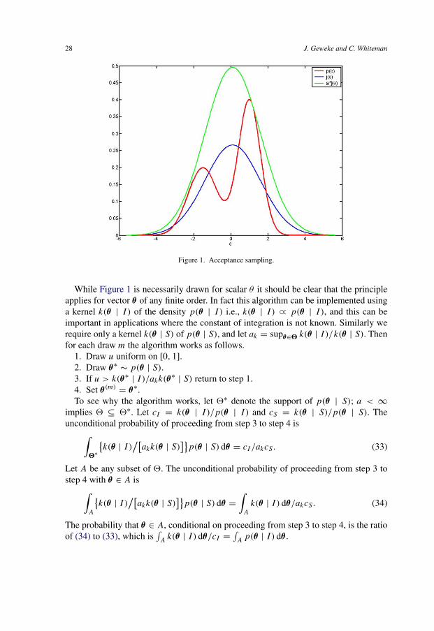
Figure 1 provides the intuition of acceptance sampling. The heavy curve is the tar-get density p(θ | I ), and the lower bell-shaped curve is the source density p(θ | S).The ratio p(θ | I )/p(θ | S) is bounded above by a constant a. In Figure 1, p(1.16 |I )/p(1.16 | S) = a = 1.86, and the lightest curve is a · p(θ | S). The idea is to drawθ∗ from the source density, which has kernel a · p(θ∗ | S), but to accept the draw withprobability p(θ∗)/a · p(θ∗ | S). For example if θ∗ = 0, then the draw is accepted withprobability 0.269, whereas if θ∗ = 1.16 then the draw is accepted with probability 1.The accepted values in fact simulate i.i.d. drawings from the target density p(θ | I ).
28 J. Geweke and C. Whiteman
Figure 1. Acceptance sampling.
While Figure 1 is necessarily drawn for scalar θ it should be clear that the principleapplies for vector θ of any finite order. In fact this algorithm can be implemented usinga kernel k(θ | I ) of the density p(θ | I ) i.e., k(θ | I ) ∝ p(θ | I ), and this can beimportant in applications where the constant of integration is not known. Similarly werequire only a kernel k(θ | S) of p(θ | S), and let ak = supθ∈� k(θ | I )/k(θ | S). Thenfor each draw m the algorithm works as follows.
1. Draw u uniform on [0, 1].2. Draw θ∗
∼ p(θ | S).3. If u > k(θ∗ | I )/akk(θ∗ | S) return to step 1.4. Set θ (m) = θ∗.To see why the algorithm works, let �∗ denote the support of p(θ | S); a < ∞
implies � ⊆ �∗. Let cI = k(θ | I )/p(θ | I ) and cS = k(θ | S)/p(θ | S). Theunconditional probability of proceeding from step 3 to step 4 is
(33)∫
�∗
{k(θ | I )
/[akk(θ | S)
]}p(θ | S) dθ = cI /akcS.
Let A be any subset of �. The unconditional probability of proceeding from step 3 tostep 4 with θ ∈ A is
(34)∫
A
{k(θ | I )
/[akk(θ | S)
]}p(θ | S) dθ =
∫A
k(θ | I ) dθ/akcS.
The probability that θ ∈ A, conditional on proceeding from step 3 to step 4, is the ratioof (34) to (33), which is
∫A
k(θ | I ) dθ/cI = ∫A
p(θ | I ) dθ .
Ch. 1: Bayesian Forecasting 29
Regardless of the choices of kernels the unconditional probability in (33) iscI /akcS = infθ∈� p(θ | S)/p(θ | I ). If one wishes to generate M draws of θ using ac-ceptance sampling, the expected number of times one will have to draw u, draw θ∗, andcompute k(θ∗ | I )/[akk(θ∗ | S)] is M · supθ∈� p(θ | I )/p(θ | S). The computationalefficiency of the algorithm is driven by those θ for which p(θ | S) has the greatest rel-ative undersampling. In most applications the time consuming part of the algorithm isthe evaluation of the kernels k(θ | S) and k(θ | I ), especially the latter. (If p(θ | I ) is aposterior density, then evaluation of k(θ | I ) entails computing the likelihood function.)In such cases this is indeed the relevant measure of efficiency.
Since θ (m) iid∼ p(θ | I ), ω(m) iid
∼ p(ω | I ) = ∫�
p(θ | I )p(ω | θ , I ) dθ . Acceptancesampling is limited by the difficulty in finding an approximation p(θ | S) that is effi-cient, in the sense just described, and by the need to find ak = supθ∈� k(θ | I )/k(θ | S).While it is difficult to generalize, these tasks are typically more difficult the greater thenumber of elements of θ .
3.1.3. Importance sampling
Rather than accept only a fraction of the draws from the source density, it is possibleto retain all of them, and consistently approximate the posterior moment by appropri-ately weighting the draws. The probability density function of the source distributionis then called the importance sampling density, a term due to Hammersly and Hand-scomb (1964), who were among the first to propose the method. It appears to have beenintroduced to the econometrics literature by Kloek and van Dijk (1978).
To describe the method, denote the source density by p(θ | S) with support �∗, andan arbitrary kernel of the source density by k(θ | S) = cS · p(θ | S) for any cS �= 0.Denote an arbitrary kernel of the target density by k(θ | I ) = cI · p(θ | I ) for anycI �= 0, the i.i.d. sequence θ (m)
∼ p(θ | S), and the sequence ω(m) drawn independentlyfrom p(ω | θ (m), I ). Define the weighting function w(θ) = k(θ | I )/k(θ | S). Then theapproximation of h = E[h(ω) | I ] is
(35)h(M) =∑M
m=1 w(θ (m))h(ω(m))∑Mm=1 w(θ (m))
.
Geweke (1989a) showed that if E[h(ω) | I ] exists and is finite, and �∗ ⊇ �, thenh(M) a.s.→ h. Moreover, if var[h(ω) | I ] exists and is finite, and if w(θ) is bounded aboveon �, then the accuracy of the approximation can be assessed using the Lindeberg–Levycentral limit theorem with an appropriately approximated variance [see Geweke (1989a,Theorem 2) or Geweke (2005, Theorem 4.2.2)]. In applications of importance sampling,this accuracy can be summarized in terms of the numerical standard error of h(M), itssampling standard deviation in independent runs of length M of the importance sam-pling simulation, and in terms of the relative numerical efficiency of h(M), the ratio ofsimulation size in a hypothetical direct simulator to that required using importance sam-pling to achieve the same numerical standard error. These summaries of accuracy can be
30 J. Geweke and C. Whiteman
used with other simulation methods as well, including the Markov chain Monte Carloalgorithms described in Section 3.2.
To see why importance sampling produces a simulation-consistent approximation ofE[h(ω) | I ], notice that
E[w(θ) | S
] =∫
�
k(θ | I )
k(θ | S)p(θ | S) dθ = cI
cS
≡ w.
Since {ω(m)} is i.i.d. the strong law of large numbers implies
(36)M−1M∑
m=1
w(θ (m)
) a.s.→ w.
The sequence {w(θ (m)), h(ω(m))} is also i.i.d., and
E[w(θ)h(ω) | I
] =∫
�
w(θ)
[∫�
h(ω)p(ω | θ , I ) dω
]p(θ | S) dθ
= (cI /cS)
∫�
∫�
h(ω)p(ω | θ , I )p(θ | I ) dω dθ
= (cI /cS)E[h(ω) | I
] = w · h.
By the strong law of large numbers,
(37)M−1M∑
m=1
w(θ (m)
)h(ω(m)
) a.s.→ w · h.
The fraction in (35) is the ratio of the left-hand side of (37) to the left-hand side of (36).One of the attractive features of importance sampling is that it requires only that
p(θ | I )/p(θ | S) be bounded, whereas acceptance sampling requires that the supre-mum of this ratio (or that for kernels of the densities) be known. Moreover, the knownsupremum is required in order to implement acceptance sampling, whereas the bound-edness of p(θ | I )/p(θ | S) is utilized in importance sampling only to exploit a centrallimit theorem to assess numerical accuracy. An important application of importancesampling is in providing remote clients with a simple way to revise prior distributions,as discussed below in Section 3.3.2.
3.2. Markov chain Monte Carlo
Markov chain Monte Carlo (MCMC) methods are generalizations of direct sampling.The idea is to construct a Markov chain {θ (m)} with continuous state space � and uniqueinvariant probability density p(θ | I ). Following an initial transient or burn-in phase,the distribution of θ (m) is approximately that of the density p(θ | I ). The exact sensein which this approximation holds is important. We shall touch on this only briefly; forfull detail and references see Geweke (2005, Section 3.5). We continue to assume that
Ch. 1: Bayesian Forecasting 31
ω can be simulated directly from p(ω | θ , I ), so that given {θ (m)} the correspondingω(m)
∼ p(ω | θ (m), I ) can be drawn.Markov chain methods have a history in mathematical physics dating back to the al-
gorithm of Metropolis et al. (1953). This method, which was described subsequentlyin Hammersly and Handscomb (1964, Section 9.3) and Ripley (1987, Section 4.7),was generalized by Hastings (1970), who focused on statistical problems, and was fur-ther explored by Peskun (1973). A version particularly suited to image reconstructionand problems in spatial statistics was introduced by Geman and Geman (1984). Thiswas subsequently shown to have great potential for Bayesian computation by Gelfandand Smith (1990). Their work, combined with data augmentation methods [see Tannerand Wong (1987)] has proven very successful in the treatment of latent variables ineconometrics. Since 1990 application of MCMC methods has grown rapidly: new re-finements, extensions, and applications appear constantly. Accessible introductions areGelman et al. (1995), Chib and Greenberg (1995) and Geweke (2005); a good collec-tion of applications is Gilks, Richardson and Spiegelhaldter (1996). Section 5 providesseveral applications of MCMC methods in Bayesian forecasting models.
3.2.1. The Gibbs sampler
Most posterior densities p(θA | YoT , A) do not correspond to any conventional family
of distributions. On the other hand, the conditional distributions of subvectors of θA
often do, which is to say that the conditional posterior distributions of these subvectorsare conventional. This is partially the case in the stochastic volatility model describedin Section 2.1.2. If, for example, the prior distribution of φ is truncated Gaussian andthose of β2 and σ 2
η are inverted gamma, then the conditional posterior distribution ofφ is truncated normal and those of β2 and σ 2
η are inverted gamma. (The conditionalposterior distributions of the latent volatilities ht are unconventional, and we return tothis matter in Section 5.5.)
This motivates the simplest setting for the Gibbs sampler. Suppose θ ′ = (θ ′1, θ
′2)
has density p(θ1, θ2 | I ) of unconventional form, but that the conditional densitiesp(θ1 | θ2, I ) and p(θ2 | θ1, I ) are conventional. Suppose (hypothetically) that one hadaccess to an initial drawing θ
(0)2 taken from p(θ2 | I ), the marginal density of θ2. Then
after iterations θ(m)1 ∼ p(θ1 | θ
(m−1)2 , I ), θ
(m)2 ∼ p(θ2 | θ
(m)1 , I ) (m = 1, . . . ,M) one
would have a collection θ (m) = (θ′(m)1 , θ
′(m)2 )′ ∼ p(θ | I ). The extension of this idea
to more than two components of θ , given a blocking θ ′ = (θ ′1, . . . , θ
′B) and an initial
θ (0)∼ p(θ | I ), is immediate, cycling through
θ(m)b ∼ p
[θ (b)
∣∣ θ (m)a (a < b), θ (m−1)
a (a > b), I]
(38)(b = 1, . . . , B; m = 1, 2, . . .).
Of course, if it were possible to make an initial draw from this distribution, thenindependent draws directly from p(θ | I ) would also be possible. The purpose of thatassumption here is to marshal an informal argument that the density p(θ | I ) is an
32 J. Geweke and C. Whiteman
invariant density of this Markov chain: that is, if θ (m)∼ p(θ | I ), then θ (m+s)
∼
p(θ | I ) for all s > 0.It is important to elucidate conditions for θ (m) to converge in distribution to p(θ | I )
given any θ (0) ∈ �. Note that even if θ (0) were drawn from p(θ | I ), the argumentjust given demonstrates only that any single θ (m) is also drawn from p(θ | I ). It doesnot establish that a single sequence {θ (m)} is representative of p(θ | I ). Consider theexample shown in Figure 2(a), in which � = �1 ∪ �2, and the Gibbs sampling al-gorithm has blocks θ1 and θ2. If θ (0) ∈ �1, then θ (m) ∈ �1 for m = 1, 2, . . . . Anysingle θ (m) is just as representative of p(θ | I ) as is the single drawing θ (0), but thesame cannot be said of the collection {θ (m)}. Indeed, {θ (m)} could be highly mislead-ing. In the example shown in Figure 2(b), if θ (0) is the indicated point at the lowerleft vertex of the triangular closed support of p(θ | I ), then θ (m) = θ (0) ∀m. Whatis required is that the Gibbs sampling Markov chain {θ (m)} with transition densityp(θ (m) | θ (m−1),G) defined in (38) be ergodic. That is, if ω(m)
∼ p(ω | θ , I ) andE[h(θ ,ω) | I ] exists, then we require M−1∑M
m=1 h(θ (m),ω(m))a.s.→ E[h(θ ,ω) | I ].
Careful statement of the weakest sufficient conditions demands considerably more the-oretical apparatus than can be developed here; for this, see Tierney (1994). Somewhat
Figure 2. Two examples in which a Gibbs sampling Markov chain will be reducible.
Ch. 1: Bayesian Forecasting 33
stronger, but still widely applicable, conditions are easier to state. For example, if forany Lebesgue measurable A with
∫A
p(θ | I ) dθ > 0 it is the case that in the Markovchain (38) P(θ (m+1) ∈ A | θ (m),G) > 0 for any θ (m) ∈ �, then the Markov chain isergodic. (Clearly neither example in Figure 2 satisfies this condition.) For this and othersimple conditions see Geweke (2005, Section 4.5).
3.2.2. The Metropolis–Hastings algorithm
The Metropolis–Hastings algorithm is defined by a probability density function p(θ∗ |θ ,H) indexed by θ ∈ � and with density argument θ∗. The random vector θ∗ generatedfrom p(θ∗ | θ (m−1), H) is a candidate value for θ (m). The algorithm sets θ (m) = θ∗ withprobability
(39)α(θ∗ | θ (m−1), H
) = min
{p(θ∗ | I )/p(θ∗ | θ (m−1), H)
p(θ (m−1) | I )/p(θ (m−1) | θ∗,H), 1
};
otherwise, θ (m) = θ (m−1). Conditional on θ = θ (m−1) the distribution of θ∗ is a mixtureof a continuous distribution with density given by u(θ∗ | θ ,H) = p(θ∗ | θ ,H)α(θ∗ |θ ,H), corresponding to the accepted candidates, and a discrete distribution with proba-bility mass r(θ | H) = 1 − ∫
�u(θ∗ | θ ,H) dθ∗ at the point θ , which is the probability
of drawing a θ∗ that will be rejected. The entire transition density can be expressedusing the Dirac delta function as
(40)p(θ (m) | θ (m−1), H
) = u(θ (m) | θ (m−1), H
)+ r(θ (m−1) | H
)δθ (m−1)
(θ (m)
).
The intuition behind this procedure is evident on the right-hand side of (39), and is inmany respects similar to that in acceptance and importance sampling. If the transitiondensity p(θ∗ | θ ,H) makes a move from θ (m−1) to θ∗ quite likely, relative to the targetdensity p(θ | I ) at θ∗, and a move back from θ∗ to θ (m−1) quite unlikely, relative tothe target density at θ (m−1), then the algorithm will place a low probability on actuallymaking the transition and a high probability on staying at θ (m−1). In the same situation,a prospective move from θ∗ to θ (m−1) will always be made because draws of θ (m−1) aremade infrequently relative to the target density p(θ | I ).
This is the most general form of the Metropolis–Hastings algorithm, due to Hastings(1970). The Metropolis et al. (1953) form takes p(θ∗ | θ,H) = p(θ | θ∗,H), whichin turn leads to a simplification of the acceptance probability: α(θ∗ | θ (m−1), H) =min[p(θ∗ | I )/p(θ (m−1) | I ), 1]. A leading example of this form is the Metropolis ran-dom walk, in which p(θ∗ | θ ,H) = p(θ∗ − θ | H) and the latter density is symmetricabout 0, for example that of the multivariate normal distribution with mean 0. Anotherspecial case is the Metropolis independence chain [see Tierney (1994)] in which p(θ∗ |θ ,H) = p(θ∗ | H). This leads to α(θ∗ | θ (m−1), H) = min[w(θ∗)/w(θ (m−1)), 1],where w(θ) = p(θ | I )/p(θ | H). The independence chain is closely related to ac-ceptance sampling and importance sampling. But rather than place a low probability ofacceptance or a low weight on a draw that is too likely relative to the target distribution,the independence chain assigns a low probability of transition to that candidate.
34 J. Geweke and C. Whiteman
There is a simple two-step argument that motivates the convergence of the se-quence {θ (m)}, generated by the Metropolis–Hastings algorithm, to the distribution ofinterest. [This approach is due to Chib and Greenberg (1995).] First, note that if a transi-tion probability density function p(θ (m) | θ (m−1), T ) satisfies the reversibility condition
p(θ (m−1) | I
)p(θ (m) | θ (m−1), T
) = p(θ (m) | I
)p(θ (m−1) | θ (m), T
)with respect to p(θ | I ), then∫
�
p(θ (m−1) | I
)p(θ (m) | θ (m−1), T
)dθ (m−1)
=∫
�
p(θ (m) | I
)p(θ (m−1) | θ (m), T
)dθ (m−1)
(41)= p(θ (m) | I
) ∫�
p(θ (m−1) | θ (m), T
)dθ (m−1) = p
(θ (m) | I
).
Expression (41) indicates that if θ (m−1)∼ p(θ | I ), then the same is true of θ (m). The
density p(θ | I ) is an invariant density of the Markov chain with transition densityp(θ (m) | θ (m−1), T ).
The second step in this argument is to consider the implications of the requirementthat the Metropolis–Hastings transition density p(θ (m) | θ (m−1), H) be reversible withrespect to p(θ | I ),
p(θ (m−1) | I
)p(θ (m) | θ (m−1), H
) = p(θ (m) | I
)p(θ (m−1) | θ (m),H
).
For θ (m−1) = θ (m) the requirement holds trivially. For θ (m−1) �= θ (m) it implies that
p(θ (m−1) | I
)p(θ∗ | θ (m−1), H
)α(θ∗ | θ (m−1), H
)(42)= p
(θ∗ | I
)p(θ (m−1) | θ∗,H
)α(θ (m−1) | θ∗,H
).
Suppose without loss of generality that
p(θ (m−1) | I
)p(θ∗ | θ (m−1), H
)> p
(θ∗ | I
)p(θ (m−1) | θ∗,H
).
If α(θ (m−1) | θ∗,H) = 1 and
α(θ∗ | θ (m−1), H
) = p(θ∗ | I )p(θ (m−1) | θ∗,H)
p(θ (m−1) | I )p(θ∗ | θ (m−1), H),
then (42) is satisfied.
3.2.3. Metropolis within Gibbs
Different MCMC methods can be combined in a variety of rich and interesting waysthat have been important in solving many practical problems in Bayesian inference.One of the most important in econometric modelling has been the Metropolis withinGibbs algorithm. Suppose that in attempting to implement a Gibbs sampling algorithm,
Ch. 1: Bayesian Forecasting 35
a conditional density p[θ (b) | θ (a) (a �= b)] is intractable. The density is not of anyknown form, and efficient acceptance sampling algorithms are not at hand. This occursin the stochastic volatility example, for the volatilities h1, . . . , hT .
This problem can be addressed by applying the Metropolis–Hastings algorithm inblock b of the Gibbs sampler while treating the other blocks in the usual way. Specif-ically, let p(θ∗
(b) | θ ,Hb) be the density (indexed by θ ) from which candidate θ∗(b) is
drawn. At iteration m, block b, of the Gibbs sampler draw θ∗(b) ∼ p(θ∗
(b) | θ (m)a (a <
b), θ (m−1)a (a � b),Hb), and set θ
(m)(b) = θ∗
(b) with probability
α[θ∗
(b) | θ (m)a (a < b), θ (m−1)
a (a � b),Hb
]= min
{p[θ (m)
a (a < b), θ∗b, θ
(m−1)a (a > b) | I ]
p[θ∗(b) | θ (m)
a (a < b), θ (m−1)a (a � b),Hb]
/p[θ (m)
a (a < b), θ (m−1)a (a � b) | I ]
p[θ (m−1)b | θ (m)
a (a < b), θ∗b, θ
(m−1)a (a > b),Hb]
, 1
}.
If θ(m)(b) is not set to θ∗
(b), then θ(m)(b) = θ
(m−1)(b) . The procedure for θ (b) is exactly the same
as for a standard Metropolis step, except that θa (a �= b) also enters the density p(θ | I )
and transition density p(θ | H). It is usually called a Metropolis within Gibbs step.To see that p(θ | I ) is an invariant density of this Markov chain, consider the simple
case of two blocks with a Metropolis within Gibbs step in the second block. Adaptingthe notation of (40), describe the Metropolis step for the second block by
p(θ∗
(2) | θ (1), θ (2), H2) = u
(θ∗
(2) | θ (1), θ (2), H2)+ r(θ (2) | θ (1), H2)δθ (2)
(θ∗
(2)
)where
u(θ∗
(2) | θ (1), θ (2), H2) = α
(θ∗
(2) | θ (1), θ (2), H2)p(θ∗
(2) | θ (1), θ (2), H2)
and
(43)r(θ (2) | θ (1), H2) = 1 −∫
�2
u(θ∗
(2) | θ (1), θ (2), H2)
dθ∗(2).
The one-step transition density for the entire chain is
p(θ∗ | θ ,G
) = p(θ∗
(1) | θ (2), I)p(θ∗
(2) | θ (1), θ (2), H2).
Then p(θ | I ) is an invariant density of p(θ∗ | θ,G) if
(44)∫
�
p(θ | I )p(θ∗ | θ ,G
)dθ = p
(θ∗ | I
).
To establish (44), begin by expanding the left-hand side,∫�
p(θ | I )p(θ∗ | θ ,G
)dθ =
∫�2
∫�1
p(θ (1), θ (2) | I ) dθ (1)p(θ∗
(1) | θ (2), I)
36 J. Geweke and C. Whiteman
× [u(θ∗(2) | θ∗
(1), θ (2), H2)+ r
(θ (2) | θ∗
(1), H2)δθ (2)
(θ∗
(2)
)]dθ (2)
(45)=∫
�2
p(θ (2) | I )p(θ∗
(1) | θ (2), I)u(θ∗
(2) | θ∗(1), θ (2), H2
)dθ (2)
(46)+∫
�2
p(θ (2) | I )p(θ∗
(1) | θ (2), I)r(θ (2) | θ∗
(1), H2)δθ (2)
(θ∗
(2)
)dθ (2).
In (45) and (46) we have used the fact that
p(θ (2) | I ) =∫
�1
p(θ (1), θ (2) | I ) dθ (1).
Using Bayes rule (45) is the same as
(47)p(θ∗
(1) | I) ∫
�2
p(θ (2) | θ∗
(1), I)u(θ∗
(2) | θ∗(1), θ (2), H2
)dθ (2).
Carrying out the integration in (46) yields
(48)p(θ∗
(2) | I)p(θ∗
(1) | θ∗(2), I
)r(θ∗
(2) | θ∗(1), H2
).
Recalling the reversibility of the Metropolis step,
p(θ (2) | θ∗
(1), I)u(θ∗
(2) | θ∗(1), θ (2), H2
) = p(θ∗
(2) | θ∗(1), I
)u(θ (2) | θ∗
(1), θ∗(2), H2
)and so (47) becomes
(49)p(θ∗
(1) | I)p(θ∗
(2) | θ∗(1), I
) ∫�2
u(θ (2) | θ∗
(1), θ∗(2), H2
)dθ (2).
We can express (48) as
(50)p(θ∗
(1), θ∗(2) | I
)r(θ∗
(2) | θ∗(1), H2
).
Finally, recalling (43), the sum of (49) and (50) is p(θ∗(1), θ
∗(2) | I ), thus establish-
ing (44).This demonstration of invariance applies to the Gibbs sampler with b blocks, with
a Metropolis within Gibbs step for one block, simply through the convention thatMetropolis within Gibbs is used in the last block of each iteration. Metropolis withinGibbs steps can be used for several blocks, as well. The argument for invariance pro-ceeds by mathematical induction, and the details are the same.
Sections 5.2.1 and 5.5 provide applications of Metropolis within Gibbs in Bayesianforecasting models.
3.3. The full Monte
We are now in a position to complete the practical Bayesian agenda for forecasting bymeans of simulation. This process integrates several sources of uncertainty about thefuture. These are summarized from a non-Bayesian perspective in the most widely usedgraduate econometrics textbook [Greene (2003, p. 576)] as
Ch. 1: Bayesian Forecasting 37
(1) uncertainty about parameters (“which will have been estimated”);(2) uncertainty about forecasts of exogenous variables; and(3) uncertainty about unobservables realized in the future.
To these most forecasters would add, along with Diebold (1998, pp. 291–292) whoincludes (1) and (3) but not (2) in his list,
(4) uncertainty about the model itself.Greene (2003) points out that for the non-Bayesian forecaster, “In practice handling
the second of these errors is largely intractable while the first is merely extremelydifficult.” The problem with parameters in non-Bayesian approaches originates in theviolation of the principle of relevant conditioning, as discussed in the conclusions ofSections 2.4.2 and 2.4.3. The difficulty with exogenous variables is grounded in vio-lation of the principle of explicit formulation: a so-called exogenous variable in thissituation is one whose joint distribution with the forecasting vector of interest ω shouldhave been expressed explicitly, but was not.2 This problem is resolved every day indecision-making, either formally or informally, in any event. If there is great uncertaintyabout the joint distribution of some relevant variables and the forecasting vector of in-terest, that uncertainty should be incorporated in the prior distribution, or in uncertaintyabout the appropriate model.
We turn first to the full integration of the first three sources of uncertainty usingposterior simulators (Section 3.3.1) and then to the last source (Section 3.3.2).
3.3.1. Predictive distributions and point forecasts
Section 2.4 summarized the probability structure of the recursive formulation of a singlemodel A: the prior density p(θA | A), the density of the observables p(YT | θA,A),and the density of future observables ω, p(ω | YT , θA,A). It is straightforward tosimulate from the corresponding distributions, and this is useful in the process of modelformulation as discussed in Section 2.2. The principle of relevant conditioning, however,demands that we work instead with the distribution of the unobservables (θA and ω)conditional on the observables, YT , and the assumptions of the model, A:
p(θA,ω | YT , A) = p(θA | YT , A)p(ω | θA, YT , A).
Substituting the observed values (data) YoT for YT , we can access this distribution by
means of a posterior simulator for the first component on the right, followed by simula-tion from the predictive density for the second component:
(51)θ(m)A ∼ p
(θA | Yo
T , A), ω(m)
∼ p(ω | θ
(m)A , Yo
T , A).
2 The formal problem is that “exogenous variables” are not ancillary statistics when the vector of interestincludes future outcomes. In other applications of the same model, they may be. This distinction is clearin the Bayesian statistics literature; see, e.g., Bernardo and Smith (1994, Section 5.1.4) or Geweke (2005,Section 2.2.2).
38 J. Geweke and C. Whiteman
The first step, posterior simulation, has become practicable for most models by virtue ofthe innovations in MCMC methods summarized in Section 3.2. The second simulationis relatively simple, because it is part of the recursive formulation. The simulations θ
(m)A
from the posterior simulator will not necessarily be i.i.d. (in the case of MCMC) andthey may require weighting (in the case of importance sampling) but the simulations areergodic: i.e., so long as E[h(θA,ω) | Yo
T , A] exists and is finite,
(52)
∑Mm=1 w(m)h(θ
(m)A ,ω(m))∑M
m=1 w(m)
a.s.→ E[h(θA,ω) | Yo
T , A].
The weights w(m) in (52) come into play for importance sampling. There is anotherimportant use for weighted posterior simulation, to which we return in Section 3.3.2.
This full integration of sources of uncertainty by means of simulation appears tohave been applied for the first time in the unpublished thesis of Litterman (1979) asdiscussed in Section 4. The first published full applications of simulation methods inthis way in published papers appear to have been Monahan (1983) and Thompson andMiller (1986), which built on Thompson (1984). This study applied an autoregressivemodel of order 2 with a conventional improper diffuse prior [see Zellner (1971, p. 195)]to quarterly US unemployment rate data from 1968 through 1979, forecasting for theperiod 1980 through 1982. Section 4 of their paper outlines the specifics of (51) in thiscase. They computed posterior means of each of the 12 predictive densities, correspond-ing to a joint quadratic loss function; predictive variances; and centered 90% predictiveintervals. They compared these results with conventional non-Bayesian procedures [seeBox and Jenkins (1976)] that equate unknown parameters with their estimates, thus ig-noring uncertainty about these parameters. There were several interesting findings andcomparisons.
1. The posterior means of the parameters and the non-Bayesian point estimates aresimilar: yt = 0.441 + 1.596yt−1 − 0.669yt−2 for the former and yt = 0.342 +1.658yt−1 − 0.719yt−2 for the latter.
2. The point forecasts from the predictive density and the conventional non-Bayesianprocedure depart substantially over the 12 periods, from unemployment ratesof 5.925% and 5.904%, respectively, one-step-ahead, to 6.143% and 5.693%, re-spectively, 12 steps ahead. This is due to the fact that an F -step-ahead mean,conditional on parameter values, is a polynomial of order F in the parameter val-ues: predicting farther into the future involves an increasingly non-linear functionof parameters, and so the discrepancy between the mean of the nonlinear functionand the non-linear function of the mean also increases.
3. The Bayesian 90% predictive intervals are generally wider than the correspondingnon-Bayesian intervals; the difference is greatest 12 steps ahead, where the widthis 5.53% in the former and 5.09% in the latter. At 12 steps ahead the 90% intervalsare (3.40%, 8.93%) and (3.15%, 8.24%).
4. The predictive density is platykurtic; thus a normal approximation of the pre-dictive density (today a curiosity, in view of the accessible representation (51))
Ch. 1: Bayesian Forecasting 39
produces a 90% predictive density that is too wide, and the discrepancy increasesfor predictive densities farther into the future: 5.82% rather than 5.53%, 12 stepsahead.
Thompson and Miller did not repeat their exercise for other forecasting periods, andtherefore had no evidence on forecasting reliability. Nor did they employ the shrinkagepriors that were, contemporaneously, proving so important in the successful applicationof Bayesian vector autoregressions at the Federal Reserve Bank of Minneapolis. Wereturn to that project in Section 6.1.
3.3.2. Model combination and the revision of assumptions
Incorporation of uncertainty about the model itself is rarely discussed, and less fre-quently acted upon; Greene (2003) does not even mention it. This lacuna is rational innon-Bayesian approaches: since uncertainty cannot be integrated in the context of onemodel, it is premature, from this perspective, even to contemplate this task. Since model-specific uncertainty has been resolved, both as a theoretical and as a practical matter, inBayesian forecasting, the problem of model uncertainty is front and center. Two vari-ants on this problem are integrating uncertainty over a well-defined set of models, andbringing additional, but similar, models into such a group in an efficient manner.
Extending the expression of uncertainty to a set of J specified models is straightfor-ward in principle, as detailed in Section 2.3. From (24)–(27) it is clear that the additionaltechnical task is the evaluation of the marginal likelihoods
p(Yo
T | Aj
) =∫
�Aj
p(Yo
T | θAj, Aj
)p(θAj
| Aj) dθAj(j = 1, . . . , J ).
With few exceptions simulation approximation of the marginal likelihood is not a spe-cial case of approximating a posterior moment in the model Aj . One such exception ofpractical importance involves models Aj and Ak with a common vector of unobserv-ables θA and likelihood p(Yo
T | θA,Aj ) = p(YoT | θA,Ak) but different prior densities
p(θA | Aj) and p(θA | Ak). (For example, one model might incorporate a set of in-equality restrictions while the other does not.) If p(θA | Ak)/p(θA | Aj) is bounded
above on the support of p(θA | Aj), and if θ(m)A ∼ p(θA | Yo
T , Aj ) is ergodic then
(53)M−1M∑
m=1
p(θ
(m)A | Ak
)/p(θ
(m)A | Aj
) a.s.→ p(Yo
T | Ak
)/p(Yo
T | Aj
);see Geweke (2005, Section 5.2.1).
For certain types of posterior simulators, simulation-consistent approximation of themarginal likelihood is also straightforward: see Geweke (1989b, Section 5) or Geweke(2005, Section 5.2.2) for importance sampling, Chib (1995) for Gibbs sampling, Chiband Jeliazkov (2001) for the Metropolis–Hastings algorithm, and Meng and Wong(1996) for a general theoretical perspective. An approach that is more general, but of-ten computationally less efficient in these specific cases, is the density ratio method of
40 J. Geweke and C. Whiteman
Gelfand and Dey (1994), also described in Geweke (2005, Section 5.2.4). These ap-proaches, and virtually any conceivable approach, require that it be possible to evaluateor approximate with substantial accuracy the likelihood function. This condition is notnecessary in MCMC posterior simulators, and this fact has been central to the successof these simulations in many applications, especially those with latent variables. This,more or less, defines the rapidly advancing front of attack on this important technicalissue at the time of this writing.
Some important and practical modifications can be made to the set of models overwhich uncertainty is integrated, without repeating the exercise of posterior simulation.These modifications all exploit reweighting of the posterior simulator output. One im-portant application is updating posterior distributions with new data. In a real-timeforecasting situation, for example, one might wish to update predictive distributionsminute-by-minute, whereas as a full posterior simulation adequate for the purposes athand might take more than a minute (but less than a night). Suppose the posterior sim-ulation utilizes data through time T , but the predictive distribution is being formed attime T ∗ > T . Then
p(ω | Yo
T ∗ , A) =
∫�A
p(θA | Yo
T ∗ , A)p(ω | θA, Yo
T ∗ , A)
dθA
=∫
�A
p(θA | Yo
T , A)p(θA | Yo
T ∗ , A)
p(θA | YoT , A)
p(ω | θA, Yo
T ∗ , A)
dθA
∝∫
�A
p(θA | Yo
T , A)p(yoT +1, . . . , yo
T ∗ | θA,A)
× p(ω | θA, Yo
T ∗ , A)
dθA.
This suggests that one might use the simulator output θ (m)∼ p(θA | Yo
T , A), tak-
ing ω(m)∼ p(ω | θ
(m)A , Yo
T ∗ , A) but reweighting the simulator output to approximateE[h(ω) | Yo
T ∗ , A] by
(54)M∑
m=1
p(yoT +1, . . . , yo
T ∗ | θ(m)A ,A
)h(ω(m)
)/ M∑m=1
p(yoT +1, . . . , yo
T ∗ | θ(m)A ,A
).
This turns out to be correct; for details see Geweke (2000). One can show that (54) is asimulation-consistent approximation of E[h(ω) | Yo
T ∗ , A] and in many cases the updat-ing requires only spreadsheet arithmetic. There are central limit theorems on which tobase assessments of the accuracy of the approximations; these require more advanced,but publicly available, software; see Geweke (1999) and Geweke (2005, Sections 4.1and 5.4).
The method of reweighting can also be used to bring into the fold models withthe same likelihood function but different priors, or to explore the effect of modi-fying the prior, as (53) suggests. In that context Ak denotes the new model, with aprior distribution that is more informative in the sense that p(θA | Ak)/p(θA | Aj)
is bounded above on the support of �Aj. Reweighting the posterior simulator output
Ch. 1: Bayesian Forecasting 41
θ(m)Aj
∼ p(θAj| Yo
T , Aj ) by p(θ(m)Aj
| Ak)/p(θ(m)Aj
| Aj) provides the new simulation-consistent set of approximations. Moreover, the exercise yields the marginal likelihoodof the new model almost as a by-product, because
(55)M−1M∑
m=1
p(θ
(m)Aj
| Ak
)/p(θ
(m)Aj
| Aj
) a.s.→ p(Yo
T | Ak
)/p(Yo
T | Aj
).
This suggests a pragmatic reason for investigators to use prior distributions p(θA | Aj)
that are uninformative, in this sense: clients can tailor the simulator output to their moreinformative priors p(θA | Ak) by reweighting.
4. ’Twas not always so easy: A historical perspective
The procedures outlined in the previous section accommodate, at least in principle(and much practice), very general likelihood functions and prior distributions, primarilybecause numerical substitutes are available for analytic evaluation of expectations offunctions of interest. But prior to the advent of inexpensive desktop computing in themid-1980’s, Bayesian prediction was an analytic art. The standard econometric refer-ence for Bayesian work of any such kind was Zellner (1971), which treats predictivedensities at a level of generality similar to that in Section 2.3.2 above, and in detail forGaussian location, regression, and multiple regression problems.
4.1. In the beginning, there was diffuseness, conjugacy, and analytic work
In these specific examples, Zellner’s focus was on the diffuse prior case, which leads tothe usual normal-gamma posterior. To illustrate his approach to prediction in the normalregression model, let p = 1 and write the model (a version of Equation (1)) as
(56)YT = XT β + uT
where:• XT – a T × k matrix, with rank k, of observations on the independent variables,• β – a k × 1 vector of regression coefficients,• uT – a T ×1 vector of error terms, assumed Gaussian with mean zero and variance
matrix σ 2IT .Zellner (1971, Section 3.2) employs the “diffuse” prior specification p(β, σ ) ∝ 1
σ.
With this prior, the joint density for the parameters and the q-step prediction vectorY = {ys}T +q
s=T +1, assumed to be generated by
Y = Xβ + u,
(a version of (8)) is given by
p(Y,β, σ | YT , XT , X
) = p(Y | β, σ, X
)p(β, σ | YT , XT )
42 J. Geweke and C. Whiteman
which is the product of the conditional Gaussian predictive for Y given the parameters,and independent variables and the posterior density for β and σ , which is given by
(57)p(β, σ | YT , XT ) ∝ σ−(T +1) exp{−(YT − XT β)′(YT − XT β)/2σ 2}
and which in turn can be seen to be the product of a conditional Gaussian density for β
given σ and the data and an inverted gamma density for σ given the data. In fact, thejoint density is
p(Y,β, σ | YT , XT , X
)∝ σ−(T +q+1) exp
{− (YT − XT β)′(YT − XT β) + (Y − Xβ)′(Y − Xβ)
2σ 2
}.
To obtain the predictive density (21), p(Y | YT , XT , X), Zellner marginalizes analyti-cally rather than numerically. He does so in two steps: first, he integrates with respectto σ to obtain
p(Y,β | YT , XT , X
)∝ [(YT − XT β)′(YT − XT β) + (Y − Xβ
)′(Y − Xβ)]−(T +q)/2
and then completes the square in β, rearranges, integrates and obtains
p(Y | YT , XT , X
)∝ [Y′
T YT + Y′Y − (X′T YT + X′Y
)′M−1(X′
T YT + X′Y)]−(T −k+q)/2
where M = X′T XT +X′X. After considerable additional algebra to put this into “a more
intelligible form”, Zellner obtains
p(Y | YT , XT , X
) ∝ [T − k + (Y − Xβ)′H(Y − Xβ
)]−(T −k+q)
where β = (X′T XT )−1X′
T YT is the in-sample ordinary least squares estimator, H =(1/s2)(I − XM−1X′), and s2 = 1
T −k(YT − XT β)′H(YT − XT β). This formula is
then recognized as the multivariate Student-t density, meaning that Y is distributed assuch with mean Xβ (provided T − k > 1) and covariance matrix T −k
T −k−2 H−1 (provided
T − k > 2). Zellner notes that a linear combination of the elements of Y (his exam-ple of such a function of interest is a discounted sum) will be distributed as univariateStudent-t , so that expectations of such linear combinations can be calculated as a mat-ter of routine, but he does not elaborate further. In the multivariate regression model[Zellner (1971, Section 8.2)], similar calculations to those above lead to a generalizedor matrix Student-t predictive distribution.
Zellner’s treatment of the Bayesian prediction problem constituted the state of theart at the beginning of the 1970’s. In essence, linear models with Gaussian errorsand flat priors could be utilized, but not much more generality than this was possi-ble. Slightly greater generality was available if the priors were conjugate. Such priorsleave the posterior in the same form as the likelihood. In the Gaussian regression case,
Ch. 1: Bayesian Forecasting 43
this means a normal-gamma prior (conditional normal for the regression coefficients, in-verted gamma for the residual standard deviation) and a normal likelihood. As Section 2makes clear, there is no longer need for conjugacy and simple likelihoods, as develop-ments of the past 15 years have made it possible to replace “integration by ArnoldZellner” with “integration by Monte Carlo”, in some cases using MC methods devel-oped by Zellner himself [e.g., Zellner and Min (1995); Zellner and Chen (2001)].
4.2. The dynamic linear model
In 1976, P.J. Harrison and C.F. Stevens [Harrison and Stevens (1976)] read a paper witha title that anticipates ours before the Royal Statistical Society in which they remarkedthat “[c]ompared with current forecasting fashions our views may well appear radical”.Their approach involved the dynamic linear model (see also Chapter 7 in this volume),which is a version of a state-space observer system:
yt = x′tβ t + ut ,
β t = Gβ t−1 + wt
with utiid∼ N(0, Ut ) and wt
iid∼ N(0, Wt ). Thus the slope parameters are treated as latent
variables, as in Section 2.2.4. As Harrison and Stevens note, this generalizes the stan-dard linear Gaussian model (one of Zellner’s examples) by permitting time variationin β and the residual covariance matrix. Starting from a prior distribution for β0 Harri-son and Stevens calculate posterior distributions for β t for t = 1, 2, . . . via the (now)well-known Kalman filter recursions. They also discuss prediction formulae for yT +k
at time T under the assumption (i) that xT +k is known at T , and (ii) xT +k is unknownat T . They note that their predictions are “distributional in nature, and derived from thecurrent parameter uncertainty” and that “[w]hile it is natural to think of the expectationsof the future variate values as “forecasts” there is no need to single out the expectationfor this purpose . . . if the consequences of an error in one direction are more seriousthat an error of the same magnitude in the opposite direction, then the forecast can bebiased to take this into account” (cf. Section 2.4.1).
Harrison and Stevens take up several examples, beginning with the standard regres-sion model, the “static case”. They note that in this context, their Bayesian–Kalmanfilter approach amounts to a
computationally neat and economical method of revising regression coefficientestimates as fresh data become available, without effectively re-doing the wholecalculation all over again and without any matrix inversion. This has been previ-ously pointed out by Plackett (1950) and others but its practical importance seemsto have been almost completely missed. (p. 215)
Other examples they treat include the linear growth model, additive seasonal model,periodic function model, autoregressive models, and moving average models. They alsoconsider treatment of multiple possible models, and integrating across them to obtainpredictions, as in Section 2.3.
44 J. Geweke and C. Whiteman
Note that the Harrison–Stevens approach generalized what was possible using Zell-ner’s (1971) book, but priors were still conjugate, and the underlying structure was stillGaussian. The structures that could be handled were more general, but the statistical as-sumptions and nature of prior beliefs accommodated were quite conventional. Indeed,in his discussion of Harrison–Stevens, Chatfield (1976) remarks that
. . . you do not need to be Bayesian to adopt the method. If, as the authors suggest,the general purpose default priors work pretty well for most time series, then onedoes not need to supply prior information. So, despite the use of Bayes’ theoreminherent in Kalman filtering, I wonder if Adaptive Forecasting would be a betterdescription of the method. (p. 231)
The fact remains, though, that latent-variable structure of the forecasting model doesput uncertainty about the parameterization on a par with the uncertainty associated withthe stochastic structure of the observables themselves.
4.3. The Minnesota revolution
During the mid- to late-1970’s, Christopher Sims was writing what would become“Macroeconomics and reality”, the lead article in the January 1980 issue of Economet-rica. In that paper, Sims argued that identification conditions in conventional large-scaleeconometric models that were routinely used in (non Bayesian) forecasting and policyexercises, were “incredible” – either they were normalizations with no basis in theory,or “based” in theory that was empirically falsified or internally inconsistent. He pro-posed, as an alternative, an approach to macroeconomic time series analysis with littletheoretical foundation other than statistical stationarity. Building on the Wold decom-position theorem, Sims argued that, exceptional circumstances aside, vectors of timeseries could be represented by an autoregression, and further, that such representationscould be useful for assessing features of the data even though they reproduce only thefirst and second moments of the time series and not the entire probabilistic structure or“data generation process”.
With this as motivation, Robert Litterman (1979) took up the challenge of devisingprocedures for forecasting with such models that were intended to compete directly withlarge-scale macroeconomic models then in use in forecasting. Betraying a frequentistbackground, much of Litterman’s effort was devoted to dealing with “multicollinearityproblems and large sampling errors in estimation”. These “problems” arise becausein (3), each of the equations for the p variables involves m lags of each of p variables,resulting in mp2 coefficients in B1, . . . , Bm. To these are added the parameters BD
associated with the deterministic components, as well as the p(p+1) distinct parametersin �.
Litterman (1979) treats these problems in a distinctly classical way, introducing “re-strictions in the form of priors” in a subsection on “Biased estimation”. While he notesthat “each of these methods may be given a Bayesian interpretation”, he discusses re-duction of sampling error in classical estimation of the parameters of the normal linear
Ch. 1: Bayesian Forecasting 45
model (56) via the standard ridge regression estimator [Hoerl and Kennard (1970)]
βkR = (X′
T XT + �Ik
)−1X′T YT ,
the Stein (1974) class
βkS = (X′
T XT + �X′T XT
)−1X′T YT ,
and, following Maddala (1977), the “generalized ridge”
(58)βkS = (X′
T XT + ��−1)−1(X′T YT + ��−1θ
).
Litterman notes that the latter “corresponds to a prior distribution on β of N(θ, λ2�)
with � = σ 2/λ2”. (Both parameters σ 2 and λ2 are treated as known.) Yet Litterman’snext statement is frequentist: “The variance of this estimator is given by σ 2(X′
T XT +��−1)−1”. It is clear from his development that he has the “Bayesian” shrinkage inmind as a way of reducing the sampling variability of otherwise frequentist estimators.
Anticipating a formulation to come, Litterman considers two shrinkage priors (whichhe refers to as “generalized ridge estimators”) designed specifically with lag distribu-tions in mind. The canonical distributed lag model for scalar y and x is given by
(59)yt = α + β0xt + β1xt−1 + · · · + βlxt−m + ut .
The first prior, due to Leamer (1972), shrinks the mean and variance of the lag co-efficients at the same geometric rate with the lag, and covariances between the lagcoefficients at a different geometric rate according to the distance between them:
Eβi = υρi,
cov(βi, βj ) = λ2ω|i−j |ρi+j−2
with 0 < ρ,ω < 1. The hyperparameters ρ, and ω control the decay rates, while υ
and λ control the scale of the mean and variance. The spirit of this prior lives on in the“Minnesota” prior to be discussed presently.
The second prior is Shiller’s (1973) “smoothness” prior, embodied by
(60)R[β1, . . . , βm]′ = w, w ∼ N(0, σ 2
wIm−2)
where the matrix R incorporates smoothness restrictions by “differencing” adjacentlag coefficients; for example, to embody the notion that second differences between lagcoefficients are small (that the lag distribution is quadratic), R is given by
R =
⎡⎢⎢⎢⎣1 −2 1 0 0 . . . 00 1 −2 1 0 0 . . . 0
. . .. . .
. . .. . .
0 0 . . . 1 −2 1
⎤⎥⎥⎥⎦ .
Having introduced these priors, Litterman dismisses the latter, quoting Sims: “. . . thewhole notion that lag distributions in econometrics ought to be smooth is . . . at best
46 J. Geweke and C. Whiteman
weakly supported by theory or evidence” [Sims (1974, p. 317)]. In place of a smooth lagdistribution, Litterman (1979, p. 20) assumed that “a reasonable approximation of thebehavior of an economic variable is a random walk around an unknown, deterministiccomponent”. Further, Litterman operated equation by equation, and therefore assumedthat the parameters for equation i of the autoregression (3) were centered around
yit = yi,t−1 + dit + εit .
Litterman goes on to describe the prior:
The parameters are all assumed to have means of zero except the coefficient onthe first lag of the dependent variable, which is given a prior mean of one. Theparameters are assumed to be uncorrelated with each other and to have standarddeviations which decrease the further back they are in the lag distributions. Ingeneral, the prior distribution on lag coefficients of the dependent variable is muchlooser, that is, has larger standard deviations, than it is on other variables in thesystem. (p. 20)
A footnote explains that while the prior represents Litterman’s opinion, “it was de-veloped with the aid of many helpful suggestions from Christopher Sims” [Litterman(1979, p. 96)]. Inasmuch as these discussions and the prior development took place dur-ing the course of Litterman’s dissertation work at the University of Minnesota underSims’s direction, the prior has come to be known as the “Minnesota” or “Litterman”prior. Prior information on deterministic components is taken to be diffuse, though hedoes use the simple first order stationary model
y1t = α + βy1,t−1 + ε1t
to illustrate the point that the mean M1 = E(y1t ) and persistence (β) are related byM1 = α/(1 − β), indicating that priors on the deterministic components independentof the lag coefficients are problematic. This notion was taken up by Schotman and vanDijk (1991) in the unit root literature.
The remainder of the prior involves the specification of the standard deviation of thecoefficient on lag l of variable j in equation i: δl
ij . This is specified by
(61)δlij =
⎧⎪⎪⎨⎪⎪⎩λ
lγ1if i = j,
λγ2σi
lγ1 σj
if i �= j
where γ1 is a hyperparameter greater than 1.0, γ2 and λ are scale factors, and σi and σj
are the estimated residual standard deviations in unrestricted ordinary least squares es-timates of equations i and j of the system. [In subsequent work, e.g., Litterman (1986),the residual standard deviation estimates were from univariate autoregressions.] Alter-natively, the prior can be expressed as
(62)Riβi = ri + vi , vi ∼ N(0, λ2Imp
)
Ch. 1: Bayesian Forecasting 47
where β i represents the lag coefficients in equation i (the ith row of B1, B2, . . . , Bl inEquation (3)), Ri is a diagonal matrix with zeros corresponding to deterministic com-ponents and elements λ/δl
ij corresponding to the lth lag of variable j , and ri is a vectorof zeros except for a one corresponding to the first lag of variable i. Note that specifica-tion of the prior involves choosing the prior hyperparameters for “overall tightness” λ,the “decay” γ1, and the “other’s weight” γ2. Subsequent modifications and embellish-ments (encoded in the principal software developed for this purpose, RATS) involvedalternative specifications for the decay rate (harmonic in place of geometric), and gen-eralizations of the meaning of “other” (some “others” are more equal than others).
Litterman is careful to note that the prior is being applied equation by equation, andthat he will “indeed estimate each equation separately”. Thus the prior was to be imple-mented one equation at a time, with known parameter values in the mean and variance;this meant that the “estimator” corresponded to Theil’s (1963) mixed estimator, whichcould be implemented using the generalized ridge formula (58). With such an estimator,B = (BD, B1, . . . , Bm), forecasts were produced recursively via (3). Thus the one-step-ahead forecast so produced will correspond to the mean of the predictive density, butensuing steps will not owing to the nonlinear interactions between forecasts and the Bj s.(For an example of the practical effect of this phenomenon, see Section 3.3.1.)
Litterman noted a possible loss of “efficiency” associated with his equation-by-equation treatment, but argued that the loss was justified because of the “computationalburden” of a full system treatment, due to the necessity of inverting the large cross-product matrix of right-hand-side variables. This refers to the well-known result thatequation-by-equation ordinary least squares estimation is sampling-theoretic efficientin the multiple linear regression model when the right-hand-side variables are the samein all equations. Unless � is diagonal, this does not hold when the right-hand-side vari-ables differ across equations. This, coupled with the way the prior was implementedled Litterman to reason that a system method would be more “efficient”. To see this,suppose that p > 1 in (3), stack observations on variable i in the T × 1 vector YiT ,the T × pm + d matrix with row t equal to (D′
t , y′t−1, . . . , y
′t−m) as XT and write the
equation i analogue of (56) as
(63)YiT = XT β i + uiT .
Obtaining the posterior mean associated with the prior (62) is straightforward usinga “trick” of mixed estimation: simply append “dummy variables” ri to the bottom of YiT
and Ri to the bottom of XT , and apply OLS to the resulting system. This produces theappropriate analogue of (58). But now the right-hand-side variables for equation i areof the form[
XT
Ri
]which are of course not the same across equations. In a sampling-theory context withmultiple equations with explanatory variables of this form, the “efficient” estimatoris the seemingly-unrelated-regression [see Zellner (1971)] estimator, which is not the
48 J. Geweke and C. Whiteman
same as OLS applied equation-by-equation. In the special case of diagonal �, however,equation-by-equation calculations are sufficient to compute the posterior mean of theVAR parameters. Thus Litterman’s (1979) “loss of efficiency” argument suggests that aperceived computational burden in effect forced him to make unpalatable assumptionsregarding the off-diagonal elements of �.
Litterman also sidestepped another computational burden (at the time) of treatingthe elements of the prior as unknown. Indeed, the use of estimated residual standarddeviations in the specification of the prior is an example of the “empirical” Bayesianapproach. He briefly discussed the difficulties associated with treating the parametersof the prior as unknown, but argued that the required numerical integration of the re-sulting distribution (the diffuse prior version of which is Zellner’s (57) above) was “notfeasible”. As is clear from Section 2 above (and 5 below), ten years later, feasibility wasnot a problem.
Litterman implemented his scheme on a three-variable VAR involving real GNP, M1,and the GNP price deflator using a quarterly sample from 1954:1 to 1969:4, and aforecast period 1970:1 to 1978:1. In undertaking this effort, he introduced a recursiveevaluation procedure. First, he estimated the model (obtained B) using data through1969:4 and made predictions for 1 through K steps ahead. These were recorded, thesample updated to 1970:1, the model re-estimated, and the process was repeated foreach quarter through 1977:4. Various measures of forecast accuracy (mean absolute er-ror, root mean squared error, and Theil’s U – the ratio of the root mean squared errorto that of a no-change forecast) were then calculated for each of the forecast horizons 1through K . Estimation was accomplished by the Kalman filter, though it was used onlyas a computational device, and none of its inherent Bayesian features were utilized.Litterman’s comparison to McNees’s (1975) forecast performance statistics for severallarge-scale macroeconometric models suggested that the forecasting method workedwell, particularly at horizons of about two to four quarters.
In addition to traditional measures of forecast accuracy, Litterman also devoted sub-stantial effort to producing Fair’s (1980) “estimates of uncertainty”. These are measuresof forecast accuracy that embody adjustments for changes in the variances of the fore-casts over time. In producing these measures for his Bayesian VARs, Litterman antici-pated much of the essence of posterior simulation that would be developed over the nextfifteen years. The reason is that Fair’s method decomposes forecast uncertainty into sev-eral sources, of which one is the uncertainty due to the need to estimate the coefficientsof the model. Fair’s version of the procedure involved simulation from the frequentistsampling distribution of the coefficient estimates, but Litterman explicitly indicated theneed to stochastically simulate from the posterior distribution of the VAR parameters aswell as the distribution of the error terms. Indeed, he generated 50 (!) random samplesfrom the (equation-by-equation, empirical Bayes’ counterpart to the) predictive den-sity for a six variable, four-lag VAR. Computations required 1024 seconds on the CDCCyber 172 computer at the University of Minnesota, a computer that was fast by thestandards of the time.
Ch. 1: Bayesian Forecasting 49
Doan, Litterman and Sims (1984, DLS) built on Litterman, though they retained theequation-by-equation mode of analysis he had adopted. Key innovations included ac-commodation of time variation via a Kalman filter procedure like that used by Harrisonand Stevens (1976) for the dynamic linear model discussed above, and the introduc-tion of new features of the prior to reflect views that sums of own lag coefficients ineach equation equal unity, further reflecting the random walk prior. [Sims (1992) sub-sequently introduced a related additional feature of the prior reflecting the view thatvariables in the VAR may be cointegrated.]
After searching over prior hyperparameters (overall tightness, degree of time varia-tion, etc.) DLS produced a “prior” involving small time variation and some “bite” fromthe sum-of-lag coefficients restriction that improved pseudo-real time forecast accuracymodestly over univariate predictions for a large (10 variable) model of macroeconomictime series. They conclude the improvement is “. . . substantial relative to differences inforecast accuracy ordinarily turned up in comparisons across methods, even though it isnot large relative to total forecast error.” (pp. 26–27)
4.4. After Minnesota: Subsequent developments
Like DLS, Kadiyala and Karlsson (1993) studied a variety of prior distributions formacroeconomic forecasting, and extended the treatment to full system-wide analysis.They began by noting that Litterman’s (1979) equation-by-equation formulation has aninterpretation as a multivariate analysis, albeit with a Gaussian prior distribution forthe VAR coefficients characterized by a diagonal, known, variance-covariance matrix.(In fact, this “known” covariance matrix is data determined owing to the presence ofestimated residual standard deviations in Equation (61).) They argue that diagonality isa more troublesome assumption (being “rarely supported by data”) than the one that thecovariance matrix is known, and in any case introduce four alternatives that relax themboth.
Horizontal concatenation of equations of the form (63) and then vertically stacking(vectorizing) yields the Kadiyala and Karlsson (1993) formulation
(64)yT = (Ip ⊗ XT )b + UT
where now yT = vec(Y1T , Y2T , . . . , YpT ), b = vec(β1,β2, . . . ,βp), and UT =vec(u1T , u2T , . . . , upT ). Here UT ∼ N(0,�⊗IT ). The Minnesota prior treats var(uiT )
as fixed (at the unrestricted OLS estimate σi) and � as diagonal, and takes, for autore-gression model A,
βi | A ∼ N(βi,i )
where βi
and i are the prior mean and covariance hyperparameters. This formulationresults in the Gaussian posteriors
βi | yT , A ∼ N(βi , i
)
50 J. Geweke and C. Whiteman
where (recall (58))
β i = i
(−1
i βi+ σ−1
i X′T YiT
),
i = (−1i + σ−1
i X′T XT
)−1.
Kadiyala and Karlsson’s first alternative is the “normal-Wishart” prior, which takesthe VAR parameters to be Gaussian conditional on the innovation covariance matrix,and the covariance matrix not to be known but rather given by an inverted Wishartrandom matrix:
b | � ∼ N(b,� ⊗ �),(65)
� ∼ IW(�, α)
where the inverse Wishart density for � given degrees of freedom parameter α and“shape” � is proportional to |�|−(α+p+1)/2 exp{−0.5tr�−1�} [see, e.g., Zellner (1971,p. 395)]. This prior is the natural conjugate prior for b,�. The posterior is given by
b | �, yT, A ∼ N(b,� ⊗ �
),
� | yT, A ∼ IW(�, T + α
)where the posterior parameters b, �, and � are simple (though notationally cumber-some) functions of the data and the prior parameters b, �, and �. Simple functionsof interest can be evaluated analytically under this posterior, and for more complicatedfunctions, evaluation by posterior simulation is trivial given the ease of sampling fromthe inverted Wishart [see, e.g., Geweke (1988)].
But this formulation has a drawback, noted long ago by Rothenberg (1963), that theKronecker structure of the prior covariance matrix enforces an unfortunate symmetry onratios of posterior variances of parameters. To take an example, suppress deterministiccomponents (d = 0) and consider a 2-variable, 1-lag system (p = 2, m = 1):
y1t = B1,11y1t−1 + B1,12y2t−1 + ε1t ,
y2t = B1,21y1t−1 + B1,22y2t−1 + ε2t .
Let � = [ψij ] and � = [σij ]. Then the posterior covariance matrix for b =(B1,11 B1,12 B1,21 B1,22)
′ is given by
� ⊗ � =
⎡⎢⎢⎣ψ11σ11 ψ11σ12 ψ12σ11 ψ12σ12ψ11σ21 ψ11σ22 ψ12σ21 ψ12σ22ψ21σ11 ψ21σ12 ψ22σ11 ψ22σ12ψ21σ21 ψ21σ22 ψ22σ21 ψ22σ22
⎤⎥⎥⎦ ,
so that
var(B1,11)/var(B1,21) = ψ11σ11/ψ22σ11
= var(B1,12)/var(B1,22) = ψ11σ22/ψ22σ22.
Ch. 1: Bayesian Forecasting 51
That is, under the normal-Wishart prior, the ratio of the posterior variance of the “own”lag coefficient in first equation to that of the “other” lag coefficient in second equa-tion is identical to the ratio of the posterior variance of the “other” lag coefficient infirst equation to the “own” lag coefficient in second equation: ψ11/ψ22. This is a veryunattractive feature in general, and runs counter to the spirit of the Minnesota priorview that there is greater certainty about each equation’s “own” lag coefficients than the“others”. As Kadiyala and Karlsson (1993) put it, this “force(s) us to treat all equationssymmetrically”.
Like the normal-Wishart prior, the “diffuse” prior
(66)p(b,�) ∝ |�|−(p+1)/2
results in a posterior with the same form as the likelihood, with
b | � ∼ N(b,� ⊗ (X′
TXT)−1)
where now b is the ordinary least squares (equation-by-equation, of course) estimatorof b, and the marginal density for � is again of the inverted Wishart form. Symmetrictreatment of all equations is also feature of this formulation owing to the product form ofthe covariance matrix. Yet this formulation has found application (see, e.g., Section 5.2)because its use is very straightforward.
With the “normal-diffuse” prior
b ∼ N(b,),
p(�) ∝ |�|−(p+1)/2
of Zellner (1971, p. 239), Kadiyala and Karlsson (1993) relaxed the implicit symme-try assumption at the cost of an analytically intractable posterior. Indeed, Zellner hadadvocated the prior two decades earlier, arguing that “the price is well worth paying”.Zellner’s approach to the analytic problem was to integrate � out of the joint posteriorfor b, � and to approximate the result (a product of generalized multivariate Student tand multivariate Gaussian densities) using the leading (Gaussian) term in a Taylor se-ries expansion. This approximation has a form not unlike (65), with mean given by amatrix-weighted average of the OLS estimator and the prior mean. Indeed, the similarityof Litterman’s initial attempts to treat residual variances in his prior as unknown, whichhe regarded as computationally expensive at the time, to Zellner’s straightforward ap-proximation apparently led Litterman to abandon pursuit of a fully Bayesian analysis infavor of the mixed estimation strategy. But by the time Kadiyala and Karlsson (1993)appeared, initial development of fast posterior simulators [e.g., Drèze (1977), Kloekand van Dijk (1978), Drèze and Richard (1983), and Geweke (1989a)] had occurred,and they proceeded to utilize importance-sampling-based Monte Carlo methods for thisnormal-diffuse prior and a fourth, extended natural conjugate prior [Drèze and Morales(1976)], with only a small apology: “Following Kloek and van Dijk (1978), we havechosen to evaluate Equation (5) using Monte Carlo integration instead of standard nu-merical integration techniques. Standard numerical integration is relatively inefficientwhen the integral has a high dimensionality . . .”
52 J. Geweke and C. Whiteman
A natural byproduct of the adoption of posterior simulation is the ability to work withthe correct predictive density without resort to the approximations used by Litterman(1979), Doan, Litterman and Sims (1984), and other successors. Indeed, Kadiyala andKarlsson’s (1993) Equation (5) is precisely the posterior mean of the predictive density(our (23)) with which they were working. (This is not the first such treatment, as pro-duction forecasts from full predictive densities have been issued for Iowa tax revenues(see Section 6.2) since 1990, and the shell code for carrying out such calculations in thediffuse prior case appeared in the RATS manual in the late 1980’s.)
Kadiyala and Karlsson (1993) conducted three small forecasting “horse race” com-petitions amongst the four priors, using hyperparameters similar to those recommendedby Doan, Litterman and Sims (1984). Two experiments involved quarterly CanadianM2 and real GNP from 1955 to 1977; the other involved monthly data on the U.S. priceof wheat, along with wheat export shipments and sales, and an exchange rate index forthe U.S. dollar. In a small sample of the Canadian data, the normal-diffuse prior won,followed closely by the extended-natural-conjugate and Minnesota priors; in a largerdata set, the normal-diffuse prior was the clear winner. For the monthly wheat data, noone procedure dominated, though priors that allowed for dependencies across equationparameters were generally superior.
Four years later, Kadiyala and Karlsson (1997) analyzed the same four priors, but bythen the focus had shifted from the pure forecasting performance of the various priorsto the numerical performance of posterior samplers and associated predictives. Indeed,Kadiyala and Karlsson (1997) provide both importance sampling and Gibbs samplingschemes for simulating from each of the posteriors they considered, and provide infor-mation regarding numerical efficiencies of the simulation procedures.
Sims and Zha (1999), which was submitted for publication in 1994, and Sims and Zha(1998), completed the Bayesian treatment of the VAR by generalizing procedures forimplementing prior views regarding the structure of cross-equation errors. In particular,they wrote (3) in the form
(67)C0yt = CDDt + C1yt−1 + C2yt−2 + · · · + Cmyt−m + ut
with
Eutu′t = I
which accommodates various identification schemes for C0. For example, one route forpassing from (3) to (67) is via “Choleski factorization” of as = 1/21/2′
sothat C0 = −1/2 and ut = �−1/2εt . This results in exact identification of parame-ters in C0, but other “overidentification” schemes are possible as well. Sims and Zha(1999) worked directly with the likelihood, thus implicitly adopting a diffuse prior forC0, CD, C1, . . . , Cm. They showed that conditional on C0, the posterior (“likelihood”)for the other parameters is Gaussian, but the marginal for C0 is not of any standardform. They indicated how to sample from it using importance sampling, but in applica-tion used a random walk Metropolis-chain procedure utilizing a multivariate-t candidate
Ch. 1: Bayesian Forecasting 53
generator. Subsequently, Sims and Zha (1998) showed how to adopt an informativeGaussian prior for CD, C1, . . . , Cm|C0 together with a general (diffuse or informative)prior for C0 and concluded with the “hope that this will allow the transparency and re-producibility of Bayesian methods to be more widely available for tasks of forecastingand policy analysis” (p. 967).
5. Some Bayesian forecasting models
The vector autoregression (VAR) is the best known and most widely applied Bayesianeconomic forecasting model. It has been used in many contexts, and its ability to im-prove forecasts and provide a vehicle for communicating uncertainty is by now wellestablished. We return to a specific application of the VAR illustrating these qualitiesin Section 6. In fact Bayesian inference is now widely undertaken with many models,for a variety of applications including economic forecasting. This section surveys a fewof the models most commonly used in economics. Some of these, for example ARMAand fractionally integrated models, have been used in conjunction with methods thatare not only non-Bayesian but are also not likelihood-based because of the intractabilityof the likelihood function. The technical issues that arise in numerical maximization ofthe likelihood function, on the one hand, and the use of simulation methods in comput-ing posterior moments, on the other, are distinct. It turns out, in these cases as well asin many other econometric models, that the Bayesian integration problem is easier tosolve than is the non-Bayesian optimization problem. We provide some of the details inSections 5.2 and 5.3 below.
The state of the art in inference and computation is an important determinant of whichmodels have practical application and which do not. The rapid progress in posterior sim-ulators since 1990 is an increasingly important influence in the conception and creationof new models. Some of these models would most likely never have been substantiallydeveloped, or even emerged, without these computational tools, reviewed in Section 3.An example is the stochastic volatility model, introduced in Section 2.1.2 and discussedin greater detail in Section 5.5 below. Another example is the state space model, oftencalled the dynamic linear model in the statistics literature, which is described briefly inSection 4.2 and in more detail in Chapter 7 of this volume. The monograph by Westand Harrison (1997) provides detailed development of the Bayesian formulation of thismodel, and that by Pole, West and Harrison (1994) is devoted to the practical aspects ofBayesian forecasting.
These models all carry forward the theme so important in vector autoregressions:priors matter, and in particular priors that cope sensibly with an otherwise profligate pa-rameterization are demonstrably effective in improving forecasts. That was true in theearliest applications when computational tools were very limited, as illustrated in Sec-tion 4 for VARs, and here for autoregressive leading indicator models (Section 5.1). Thisfact has become even more striking as computational tools have become more sophisti-cated. The review of cointegration and error correction models (Section 5.4) constitutes
54 J. Geweke and C. Whiteman
a case study in point. More generally models that are preferred, as indicated by Bayesfactors, should lead to better decisions, as measured by ex post loss, for the reasonsdeveloped in Sections 2.3.2 and 2.4.1. This section closes with such a comparison fortime-varying volatility models.
5.1. Autoregressive leading indicator models
In a series of papers [Garcia-Ferer et al. (1987), Zellner and Hong (1989), Zellner, Hongand Gulati (1990), Zellner, Hong and Min (1991), Min and Zellner (1993)] Zellnerand coauthors investigated the use of leading indicators, pooling, shrinkage, and time-varying parameters in forecasting real output for the major industrialized countries. Inevery case the variable modeled was the growth rate of real output; there was no pre-sumption that real output is cointegrated across countries. The work was carried outentirely analytically, using little beyond what was available in conventional software atthe time, which limited attention almost exclusively to one-step-ahead forecasts. A prin-cipal goal of these investigations was to improve forecasts significantly using relativelysimple models and pooling techniques.
The observables model in all of these studies is of the form
(68)yit = α0 +3∑
s=1
αsyi,t−s + β ′zi,t−1 + εit , εitiid∼ N
(0, σ 2),
with yit denoting the growth rate in real GNP or real GDP between year t −1 and year t
in country i. The vector zi,t−1 comprises the leading indicators. In Garcia-Ferer et al.(1987) and Zellner and Hong (1989) zit consisted of real stock returns in country i inyears t −1 and t , the growth rate in the real money supply between years t −1 and t , andworld stock return defined as the median real stock return in year t over all countriesin the sample. Attention was confined to nine OECD countries in Garcia-Ferer et al.(1987). In Zellner and Hong (1989) the list expanded to 18 countries but the originalgroup was reported separately, as well, for purposes of comparison.
The earliest study, Garcia-Ferer et al. (1987), considered five different forecastingprocedures and several variants on the right-hand-side variables in (68). The period1954–1973 was used exclusively for estimation, and one-step-ahead forecast errors wererecorded for each of the years 1974 through 1981, with estimates being updated beforeeach forecast was made. Results for root mean square forecast error, expressed in unitsof growth rate percentage, are given in Table 1. The model LI1 includes only the twostock returns in zit ; LI2 adds the world stock return and LI3 adds also the growth ratein the real money supply. The time varying parameter (TVP) model utilizes a conven-tional state-space representation in which the variance in the coefficient drift is σ 2/2.The pooled models constrain the coefficients in (68) to be the same for all countries. Inthe variant “Shrink 1” each country forecast is an equally-weighted average of the owncountry forecast and the average forecast for all nine countries; unequally-weighted
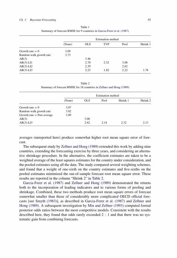
Ch. 1: Bayesian Forecasting 55
Table 1Summary of forecast RMSE for 9 countries in Garcia-Ferer et al. (1987)
Estimation method
(None) OLS TVP Pool Shrink 1
Growth rate = 0 3.09Random walk growth rate 3.73AR(3) 3.46AR(3)-LI1 2.70 2.52 3.08AR(3)-LI2 2.39 2.62AR(3)-LI3 2.23 1.82 2.22 1.78
Table 2Summary of forecast RMSE for 18 countries in Zellner and Hong (1989)
Estimation method
(None) OLS Pool Shrink 1 Shrink 2
Growth rate = 0 3.07Random walk growth rate 3.02Growth rate = Past average 3.09AR(3) 3.00AR(3)-LI3 2.62 2.14 2.32 2.13
averages (unreported here) produce somewhat higher root mean square error of fore-cast.
The subsequent study by Zellner and Hong (1989) extended this work by adding ninecountries, extending the forecasting exercise by three years, and considering an alterna-tive shrinkage procedure. In the alternative, the coefficient estimates are taken to be aweighted average of the least squares estimates for the country under consideration, andthe pooled estimates using all the data. The study compared several weighting schemes,and found that a weight of one-sixth on the country estimates and five-sixths on thepooled estimates minimized the out-of-sample forecast root mean square error. Theseresults are reported in the column “Shrink 2” in Table 2.
Garcia-Ferer et al. (1987) and Zellner and Hong (1989) demonstrated the returnsboth to the incorporation of leading indicators and to various forms of pooling andshrinkage. Combined, these two methods produce root mean square errors of forecastsomewhat smaller than those of considerably more complicated OECD official fore-casts [see Smyth (1983)], as described in Garcia-Ferer et al. (1987) and Zellner andHong (1989). A subsequent investigation by Min and Zellner (1993) computed formalposterior odds ratios between the most competitive models. Consistent with the resultsdescribed here, they found that odds rarely exceeded 2 : 1 and that there was no sys-tematic gain from combining forecasts.
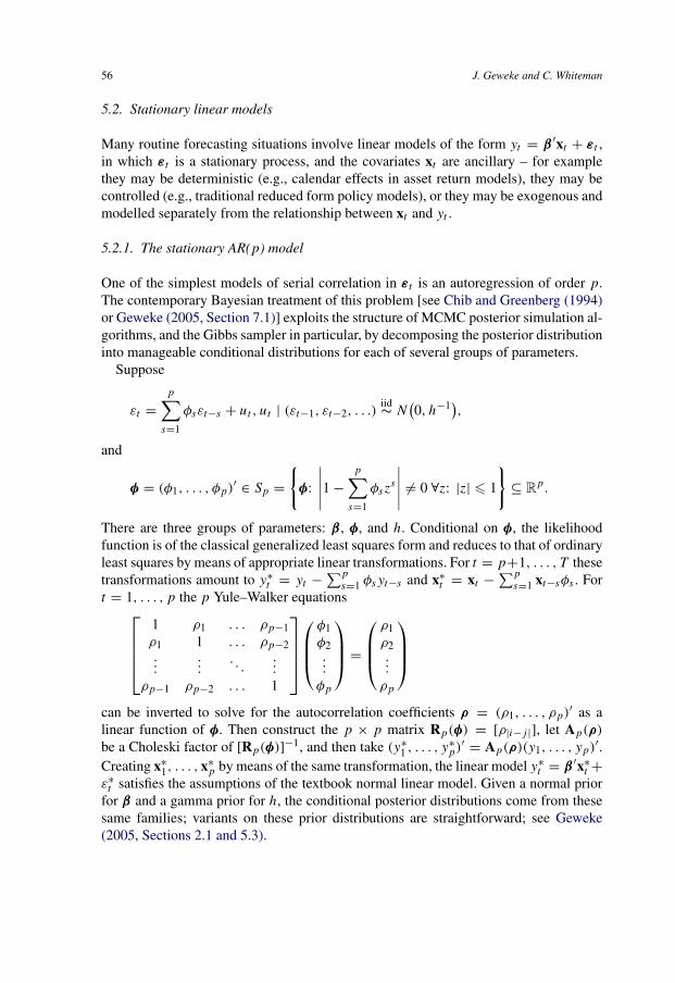
56 J. Geweke and C. Whiteman
5.2. Stationary linear models
Many routine forecasting situations involve linear models of the form yt = β ′xt + εt ,in which εt is a stationary process, and the covariates xt are ancillary – for examplethey may be deterministic (e.g., calendar effects in asset return models), they may becontrolled (e.g., traditional reduced form policy models), or they may be exogenous andmodelled separately from the relationship between xt and yt .
5.2.1. The stationary AR(p) model
One of the simplest models of serial correlation in εt is an autoregression of order p.The contemporary Bayesian treatment of this problem [see Chib and Greenberg (1994)or Geweke (2005, Section 7.1)] exploits the structure of MCMC posterior simulation al-gorithms, and the Gibbs sampler in particular, by decomposing the posterior distributioninto manageable conditional distributions for each of several groups of parameters.
Suppose
εt =p∑
s=1
φsεt−s + ut , ut | (εt−1, εt−2, . . .)iid∼ N
(0, h−1),
and
φ = (φ1, . . . , φp)′ ∈ Sp ={
φ:
∣∣∣∣∣1 −p∑
s=1
φszs
∣∣∣∣∣ �= 0 ∀z: |z| � 1
}⊆ R
p.
There are three groups of parameters: β, φ, and h. Conditional on φ, the likelihoodfunction is of the classical generalized least squares form and reduces to that of ordinaryleast squares by means of appropriate linear transformations. For t = p+1, . . . , T thesetransformations amount to y∗
t = yt −∑p
s=1 φsyt−s and x∗t = xt −∑p
s=1 xt−sφs . Fort = 1, . . . , p the p Yule–Walker equations⎡⎢⎢⎢⎣
1 ρ1 . . . ρp−1ρ1 1 . . . ρp−2...
.... . .
...
ρp−1 ρp−2 . . . 1
⎤⎥⎥⎥⎦⎛⎜⎜⎝
φ1φ2...
φp
⎞⎟⎟⎠ =
⎛⎜⎜⎝ρ1ρ2...
ρp
⎞⎟⎟⎠can be inverted to solve for the autocorrelation coefficients ρ = (ρ1, . . . , ρp)′ as alinear function of φ. Then construct the p × p matrix Rp(φ) = [ρ|i−j |], let Ap(ρ)
be a Choleski factor of [Rp(φ)]−1, and then take (y∗1 , . . . , y∗
p)′ = Ap(ρ)(y1, . . . , yp)′.Creating x∗
1, . . . , x∗p by means of the same transformation, the linear model y∗
t = β ′x∗t +
ε∗t satisfies the assumptions of the textbook normal linear model. Given a normal prior
for β and a gamma prior for h, the conditional posterior distributions come from thesesame families; variants on these prior distributions are straightforward; see Geweke(2005, Sections 2.1 and 5.3).
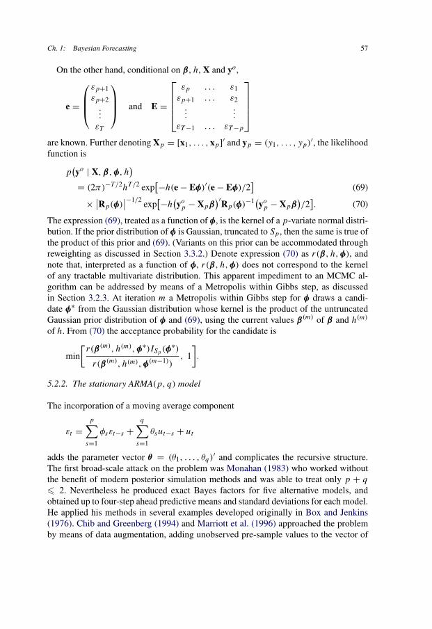
Ch. 1: Bayesian Forecasting 57
On the other hand, conditional on β, h, X and yo,
e =
⎛⎜⎜⎝εp+1εp+2
...
εT
⎞⎟⎟⎠ and E =
⎡⎢⎢⎢⎣εp . . . ε1
εp+1 . . . ε2...
...
εT −1 . . . εT −p
⎤⎥⎥⎥⎦are known. Further denoting Xp = [x1, . . . , xp]′ and yp = (y1, . . . , yp)′, the likelihoodfunction is
p(yo | X,β,φ, h
)(69)= (2π)−T/2hT/2 exp
[−h(e − Eφ)′(e − Eφ)/2]
(70)× ∣∣Rp(φ)∣∣−1/2 exp
[−h(yop − Xpβ
)′Rp(φ)−1(yop − Xpβ
)/2].
The expression (69), treated as a function of φ, is the kernel of a p-variate normal distri-bution. If the prior distribution of φ is Gaussian, truncated to Sp, then the same is true ofthe product of this prior and (69). (Variants on this prior can be accommodated throughreweighting as discussed in Section 3.3.2.) Denote expression (70) as r(β, h,φ), andnote that, interpreted as a function of φ, r(β, h,φ) does not correspond to the kernelof any tractable multivariate distribution. This apparent impediment to an MCMC al-gorithm can be addressed by means of a Metropolis within Gibbs step, as discussedin Section 3.2.3. At iteration m a Metropolis within Gibbs step for φ draws a candi-date φ∗ from the Gaussian distribution whose kernel is the product of the untruncatedGaussian prior distribution of φ and (69), using the current values β(m) of β and h(m)
of h. From (70) the acceptance probability for the candidate is
min
[r(β(m), h(m),φ∗)ISp (φ∗)
r(β(m), h(m),φ(m−1)), 1
].
5.2.2. The stationary ARMA(p, q) model
The incorporation of a moving average component
εt =p∑
s=1
φsεt−s +q∑
s=1
θsut−s + ut
adds the parameter vector θ = (θ1, . . . , θq)′ and complicates the recursive structure.The first broad-scale attack on the problem was Monahan (1983) who worked withoutthe benefit of modern posterior simulation methods and was able to treat only p + q
� 2. Nevertheless he produced exact Bayes factors for five alternative models, andobtained up to four-step ahead predictive means and standard deviations for each model.He applied his methods in several examples developed originally in Box and Jenkins(1976). Chib and Greenberg (1994) and Marriott et al. (1996) approached the problemby means of data augmentation, adding unobserved pre-sample values to the vector of
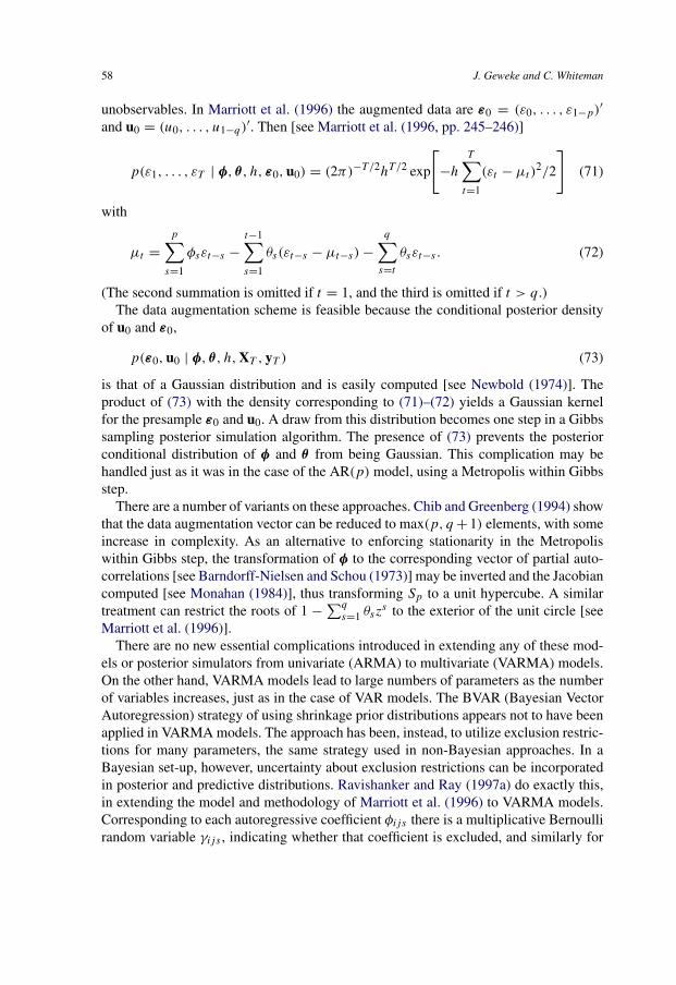
58 J. Geweke and C. Whiteman
unobservables. In Marriott et al. (1996) the augmented data are ε0 = (ε0, . . . , ε1−p)′and u0 = (u0, . . . , u1−q)′. Then [see Marriott et al. (1996, pp. 245–246)]
(71)p(ε1, . . . , εT | φ, θ , h, ε0, u0) = (2π)−T/2hT/2 exp
[−h
T∑t=1
(εt − μt)2/2
]with
(72)μt =p∑
s=1
φsεt−s −t−1∑s=1
θs(εt−s − μt−s) −q∑
s=t
θsεt−s .
(The second summation is omitted if t = 1, and the third is omitted if t > q.)The data augmentation scheme is feasible because the conditional posterior density
of u0 and ε0,
(73)p(ε0, u0 | φ, θ , h, XT , yT )
is that of a Gaussian distribution and is easily computed [see Newbold (1974)]. Theproduct of (73) with the density corresponding to (71)–(72) yields a Gaussian kernelfor the presample ε0 and u0. A draw from this distribution becomes one step in a Gibbssampling posterior simulation algorithm. The presence of (73) prevents the posteriorconditional distribution of φ and θ from being Gaussian. This complication may behandled just as it was in the case of the AR(p) model, using a Metropolis within Gibbsstep.
There are a number of variants on these approaches. Chib and Greenberg (1994) showthat the data augmentation vector can be reduced to max(p, q + 1) elements, with someincrease in complexity. As an alternative to enforcing stationarity in the Metropoliswithin Gibbs step, the transformation of φ to the corresponding vector of partial auto-correlations [see Barndorff-Nielsen and Schou (1973)] may be inverted and the Jacobiancomputed [see Monahan (1984)], thus transforming Sp to a unit hypercube. A similartreatment can restrict the roots of 1 −∑q
s=1 θszs to the exterior of the unit circle [see
Marriott et al. (1996)].There are no new essential complications introduced in extending any of these mod-
els or posterior simulators from univariate (ARMA) to multivariate (VARMA) models.On the other hand, VARMA models lead to large numbers of parameters as the numberof variables increases, just as in the case of VAR models. The BVAR (Bayesian VectorAutoregression) strategy of using shrinkage prior distributions appears not to have beenapplied in VARMA models. The approach has been, instead, to utilize exclusion restric-tions for many parameters, the same strategy used in non-Bayesian approaches. In aBayesian set-up, however, uncertainty about exclusion restrictions can be incorporatedin posterior and predictive distributions. Ravishanker and Ray (1997a) do exactly this,in extending the model and methodology of Marriott et al. (1996) to VARMA models.Corresponding to each autoregressive coefficient φijs there is a multiplicative Bernoullirandom variable γijs , indicating whether that coefficient is excluded, and similarly for
Ch. 1: Bayesian Forecasting 59
each moving average coefficient θijs there is a Bernoulli random variable δijs :
yit =n∑
j=1
p∑s=1
γijsφijsyj,t−s +n∑
j=1
q∑s=1
θijsδijsεj,t−s + εit (i = 1, . . . , n).
Prior probabilities on these random variables may be used to impose parsimony, bothglobally and also differentially at different lags and for different variables; independentBernoulli prior distributions for the parameters γijs and δijs , embedded in a hierarchicalprior with beta prior distributions for the probabilities, are the obvious alternatives to adhoc non-Bayesian exclusion decisions, and are quite tractable. The conditional posteriordistributions of the γijs and δijs are individually conditionally Bernoulli. This strategyis one of a family of similar approaches to exclusion restrictions in regression models[see George and McCulloch (1993) or Geweke (1996b)] and has also been employedin univariate ARMA models [see Barnett, Kohn and Sheather (1996)]. The posteriorMCMC sampling algorithm for the parameters φijs and δijs also proceeds one parameterat a time; Ravishanker and Ray (1997a) report that this algorithm is computationallyefficient in a three-variable VARMA model with p = 3, q = 1, applied to a data setwith 75 quarterly observations.
5.3. Fractional integration
Fractional integration, also known as long memory, first drew the attention of econo-mists because of the improved multi-step-ahead forecasts provided by even the simplestvariants of these models as reported in Granger and Joyeux (1980) and Porter-Hudak(1982). In a fractionally integrated model (1 − L)dyt = ut , where
(1 − L)d =∞∑
j=0
(d
j
)(−L)j =
∞∑j=1
(−1)j�(d − 1)
�(j − 1)�(d − j − 1)Lj
and ut is a stationary process whose autocovariance function decays geometrically. Thefully parametric version of this model typically specifies
(74)φ(L)(1 − L)d(yt − μ) = θ(L)εt ,
with φ(L) and θ(L) being polynomials of specified finite order and εt being serially
uncorrelated; most of the literature takes εtiid∼ N(0, σ 2). Sowell (1992a, 1992b) first de-
rived the likelihood function and implemented a maximum likelihood estimator. Koopet al. (1997) provided the first Bayesian treatment, employing a flat prior distributionfor the parameters in φ(L) and θ(L), subject to invertibility restrictions. This studyused importance sampling of the posterior distribution, with the prior distribution as thesource distribution. The weighting function w(θ) is then just the likelihood function,evaluated using Sowell’s computer code. The application in Koop et al. (1997) usedquarterly US real GNP, 1947–1989, a standard data set for fractionally integrated mod-els, and polynomials in φ(L) and θ(L) up to order 3. This study did not provide any
60 J. Geweke and C. Whiteman
evaluation of the efficiency of the prior density as the source distribution in the impor-tance sampling algorithm; in typical situations this will be poor if there are a half-dozenor more dimensions of integration. In any event, the computing times reported3 indicatethat subsequent more sophisticated algorithms are also much faster.
Much of the Bayesian treatment of fractionally integrated models originated withRavishanker and coauthors, who applied these methods to forecasting. Pai and Ravi-shanker (1996) provided a thorough treatment of the univariate case based on aMetropolis random-walk algorithm. Their evaluation of the likelihood function differsfrom Sowell’s. From the autocovariance function r(s) corresponding to (74) given inHosking (1981) the Levinson–Durbin algorithm provides the partial regression coeffi-cients φk
j in
(75)μt = E(yt | Yt−1) =t−1∑j=1
φt−1j yt−j .
The likelihood function then follows from
(76)yt | Yt−1 ∼ N(μt , ν
2t
), ν2
t = [r(0)/σ 2] t−1∏j=1
[1 − (φj
j
)2].
Pai and Ravishanker (1996) computed the maximum likelihood estimate as discussedin Haslett and Raftery (1989). The observed Fisher information matrix is the variancematrix used in the Metropolis random-walk algorithm, after integrating μ and σ 2 ana-lytically from the posterior distribution. The study focused primarily on inference forthe parameters; note that (75)–(76) provide the basis for sampling from the predictivedistribution given the output of the posterior simulator.
A multivariate extension of (74), without cointegration, may be expressed
�(L)D(L)(yt − μ) = �(L)εt
in which yt is n × 1, D(L) = diag[(1 − L)d1 , . . . , (1 − L)dn ], �(L) and �(L) are
n × n matrix polynomials in L of specified order, and εtiid∼ N(0,). Ravishanker and
Ray (1997b, 2002) provided an exact Bayesian treatment and a forecasting applicationof this model. Their approach blends elements of Marriott et al. (1996) and Pai andRavishanker (1996). It incorporates presample values of zt = yt − μ and the purefractionally integrated process at = D(L)−1εt as latent variables. The autocovariancefunction Ra(s) of at is obtained recursively from
ra(0)ij = σij
�(1 − di − dj )
�(1 − di)�(1 − dj ), ra(s)ij = −1 − di − s
s − dj
ra(s − 1)ij .
3 Contrast Koop et al. (1997, footnote 12) with Pai and Ravishanker (1996, p. 74).
Ch. 1: Bayesian Forecasting 61
The autocovariance function of zt is then
Rz(s) =∞∑i=1
∞∑j=0
�iRa(s + i − j)� ′j
where the coefficients �j are those in the moving average representation of the ARMApart of the process. Since these decay geometrically, truncation is not a serious issue.This provides the basis for a random walk Metropolis-within-Gibbs step constructedas in Pai and Ravishanker (1996). The other blocks in the Gibbs sampler are the pre-sample values of zt and at , plus μ and . The procedure requires on the order of n3T 2
operations and storage of order n2T 2; T = 200 and n = 3 requires a gigabyte ofstorage. If likelihood is computed conditional on all presample values being zero theproblem is computationally much less demanding, but results differ substantially.
Ravishanker and Ray (2002) provide details of drawing from the predictive den-sity, given the output of the posterior simulator. Since the presample values are aby-product of each iteration, the latent vectors at can be computed by means ofat = −∑p
i=1 izt−i+∑q
i=1 �rat−r . Then sample at forward using the autocovariancefunction of the pure long-memory process, and finally apply the ARMA recursions tothese values. The paper applies a simple version of the model (n = 3; q = 0; p = 0 or 1)to sea temperatures off the California coast. The coefficients of fractional integration areall about 0.4 when p = 0; p = 1 introduces the usual difficulties in distinguishing be-tween long memory and slow geometric decay of the autocovariance function. Thereare substantial interactions in the off-diagonal elements of (L), but the study does nottake up fractional cointegration.
5.4. Cointegration and error correction
Cointegration restricts the long-run behavior of multivariate time series that are other-wise nonstationary. Error correction models (ECMs) provide a convenient representa-tion of cointegration, and there is by now an enormous literature on inference in thesemodels. By restricting the behavior of otherwise nonstationary time series, cointegra-tion also has the promise of improving forecasts, especially at longer horizons. Cominghard on the heels of Bayesian vector autoregressions, ECMs were at first thought to becompetitors of VARs:
One could also compare these results with estimates which are obviously mis-specified such as least squares on differences or Litterman’s Bayesian Vector Au-toregression which shrinks the parameter vector toward the first difference modelwhich is itself misspecified for this system. The finding that such methods providedinferior forecasts would hardly be surprising. [Engle and Yoo (1987, pp. 151–152)]
Shoesmith (1995) carefully compared and combined the error correction specificationand the prior distributions pioneered by Litterman, with illuminating results. He used the
62 J. Geweke and C. Whiteman
quarterly, six-lag VAR in Litterman (1980) for real GNP, the implicit GNP price deflator,real gross private domestic investment, the three-month treasury bill rate and the moneysupply (M1). Throughout the exercise, Shoesmith repeatedly tested for lag length andthe outcome consistently indicated six lags. The period 1959:1 through 1981:4 was thebase estimation period, followed by 20 successive five-year experimental forecasts: thefirst was for 1982:1 through 1986:4; and the last was for 1986:4 through 1991:3 basedon estimates using data from 1959:1 through 1986:3. Error correction specification testswere conducted using standard procedures [see Johansen (1988)]. For all the samplesused, these procedures identified the price deflator as I(2), all other variables as I(1),and two cointegrating vectors.
Shoesmith compared forecasts from Litterman’s model with six other models. One,VAR/I1, was a VAR in I(1) series (i.e., first differences for the deflator and levels forall other variables) estimated by least squares, not incorporating any shrinkage or otherprior. The second, ECM, was a conventional ECM, again with no shrinkage. The otherfour models all included the Minnesota prior. One of these models, BVAR/I1, differsfrom Litterman’s model only in replacing the deflator with its first difference. Another,BECM, applies the Minnesota prior to the conventional ECM, with no shrinkage orother restrictions applied to the coefficients on the error correction terms. Yet anothervariant, BVAR/I0, applies the Minnesota prior to a VAR in I(0) variables (i.e., sec-ond differences for the deflator and first differences for all other variables). The finalmodel, BECM/5Z, is identical to BECM except that five cointegrating relationships arespecified, an intentional misreading of the outcome of the conventional procedure fordetermining the rank of the error correction matrix.
The paper offers an extensive comparison of root mean square forecasting errors forall of the variables. These are summarized in Table 3, by first forming the ratio of meansquare error in each model to its counterpart in Litterman’s model, and then averagingthe ratios across the six variables.
The most notable feature of the results is the superiority of the BECM forecasts,which is realized at all forecasting horizons but becomes greater at more distant hori-zons. The ECM forecasts, by contrast, do not dominate those of either the originalLitterman VAR or the BVAR/I1, contrary to the conjecture in Engle and Yoo (1987).The results show that most of the improvement comes from applying the Minnesotaprior to a model that incorporates stationary time series: BVAR/I0 ranks second at allhorizons, and the ECM without shrinkage performs poorly relative to BVAR/I0 at allhorizons. In fact the VAR with the Minnesota prior and the error correction models arenot competitors, but complementary methods of dealing with the profligate parameter-ization in multivariate time series by shrinking toward reasonable models with fewerparameters. In the case of the ECM the shrinkage is a hard, but data driven, restriction,whereas in the Minnesota prior it is soft, allowing the data to override in cases wherethe more parsimoniously parameterized model is less applicable. The possibilities foremploying both have hardly been exhausted. Shoesmith (1995) suggested that this maybe a promising avenue for future research.
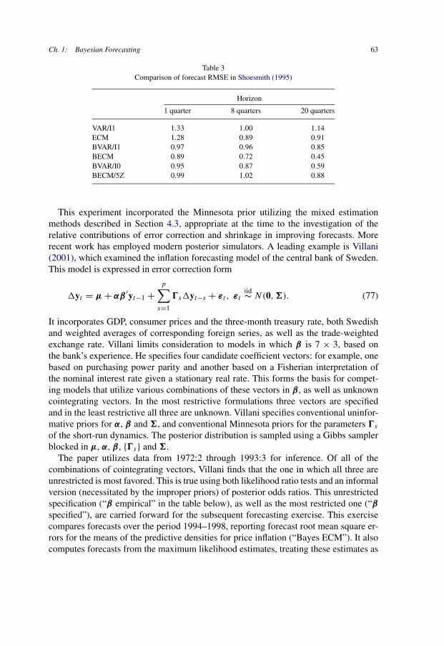
Ch. 1: Bayesian Forecasting 63
Table 3Comparison of forecast RMSE in Shoesmith (1995)
Horizon
1 quarter 8 quarters 20 quarters
VAR/I1 1.33 1.00 1.14ECM 1.28 0.89 0.91BVAR/I1 0.97 0.96 0.85BECM 0.89 0.72 0.45BVAR/I0 0.95 0.87 0.59BECM/5Z 0.99 1.02 0.88
This experiment incorporated the Minnesota prior utilizing the mixed estimationmethods described in Section 4.3, appropriate at the time to the investigation of therelative contributions of error correction and shrinkage in improving forecasts. Morerecent work has employed modern posterior simulators. A leading example is Villani(2001), which examined the inflation forecasting model of the central bank of Sweden.This model is expressed in error correction form
(77)�yt = μ + αβ ′yt−1 +p∑
s=1
�s�yt−s + εt , εtiid∼ N(0,).
It incorporates GDP, consumer prices and the three-month treasury rate, both Swedishand weighted averages of corresponding foreign series, as well as the trade-weightedexchange rate. Villani limits consideration to models in which β is 7 × 3, based onthe bank’s experience. He specifies four candidate coefficient vectors: for example, onebased on purchasing power parity and another based on a Fisherian interpretation ofthe nominal interest rate given a stationary real rate. This forms the basis for compet-ing models that utilize various combinations of these vectors in β, as well as unknowncointegrating vectors. In the most restrictive formulations three vectors are specifiedand in the least restrictive all three are unknown. Villani specifies conventional uninfor-mative priors for α, β and , and conventional Minnesota priors for the parameters �s
of the short-run dynamics. The posterior distribution is sampled using a Gibbs samplerblocked in μ, α, β, {�s} and .
The paper utilizes data from 1972:2 through 1993:3 for inference. Of all of thecombinations of cointegrating vectors, Villani finds that the one in which all three areunrestricted is most favored. This is true using both likelihood ratio tests and an informalversion (necessitated by the improper priors) of posterior odds ratios. This unrestrictedspecification (“β empirical” in the table below), as well as the most restricted one (“βspecified”), are carried forward for the subsequent forecasting exercise. This exercisecompares forecasts over the period 1994–1998, reporting forecast root mean square er-rors for the means of the predictive densities for price inflation (“Bayes ECM”). It alsocomputes forecasts from the maximum likelihood estimates, treating these estimates as
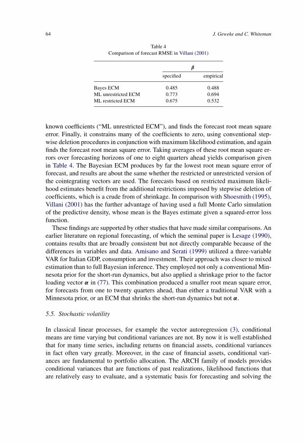
64 J. Geweke and C. Whiteman
Table 4Comparison of forecast RMSE in Villani (2001)
β
specified empirical
Bayes ECM 0.485 0.488ML unrestricted ECM 0.773 0.694ML restricted ECM 0.675 0.532
known coefficients (“ML unrestricted ECM”), and finds the forecast root mean squareerror. Finally, it constrains many of the coefficients to zero, using conventional step-wise deletion procedures in conjunction with maximum likelihood estimation, and againfinds the forecast root mean square error. Taking averages of these root mean square er-rors over forecasting horizons of one to eight quarters ahead yields comparison givenin Table 4. The Bayesian ECM produces by far the lowest root mean square error offorecast, and results are about the same whether the restricted or unrestricted version ofthe cointegrating vectors are used. The forecasts based on restricted maximum likeli-hood estimates benefit from the additional restrictions imposed by stepwise deletion ofcoefficients, which is a crude from of shrinkage. In comparison with Shoesmith (1995),Villani (2001) has the further advantage of having used a full Monte Carlo simulationof the predictive density, whose mean is the Bayes estimate given a squared-error lossfunction.
These findings are supported by other studies that have made similar comparisons. Anearlier literature on regional forecasting, of which the seminal paper is Lesage (1990),contains results that are broadly consistent but not directly comparable because of thedifferences in variables and data. Amisano and Serati (1999) utilized a three-variableVAR for Italian GDP, consumption and investment. Their approach was closer to mixedestimation than to full Bayesian inference. They employed not only a conventional Min-nesota prior for the short-run dynamics, but also applied a shrinkage prior to the factorloading vector α in (77). This combination produced a smaller root mean square error,for forecasts from one to twenty quarters ahead, than either a traditional VAR with aMinnesota prior, or an ECM that shrinks the short-run dynamics but not α.
5.5. Stochastic volatility
In classical linear processes, for example the vector autoregression (3), conditionalmeans are time varying but conditional variances are not. By now it is well establishedthat for many time series, including returns on financial assets, conditional variancesin fact often vary greatly. Moreover, in the case of financial assets, conditional vari-ances are fundamental to portfolio allocation. The ARCH family of models providesconditional variances that are functions of past realizations, likelihood functions thatare relatively easy to evaluate, and a systematic basis for forecasting and solving the
Ch. 1: Bayesian Forecasting 65
allocation problem. Stochastic volatility models provide an alternative approach, firstmotivated by autocorrelated information flows [see Tauchen and Pitts (1983)] and asdiscrete approximations to diffusion processes utilized in the continuous time asset pric-ing literature [see Hull and White (1987)]. The canonical univariate model, introducedin Section 2.1.2, is
yt = β exp(ht/2)εt , ht = φht−1 + σηηt ,
(78)h1 ∼ N[0, σ 2
η /(1 − φ2)], (εt , ηt )
′ iid∼ N(0, I2).
Only the return yt is observable. In the stochastic volatility model there are two shocksper time period, whereas in the ARCH family there is only one. As a consequence thestochastic volatility model can more readily generate extreme realizations of yt . Such arealization will have an impact on the variance of future realizations if it arises becauseof an unusually large value of ηt , but not if it is due to large εt . Because ht is a latentprocess not driven by past realizations of yt , the likelihood function cannot be evaluateddirectly. Early applications like Taylor (1986) and Melino and Turnbull (1990) usedmethod of moments rather than likelihood-based approaches.
Jacquier, Polson and Rossi (1994) were among the first to point out that the formu-lation of (78) in terms of latent variables is, by contrast, very natural in a Bayesianformulation that exploits a MCMC posterior simulator. The key insight is that condi-tional on the sequence of latent volatilities {ht }, the likelihood function for (78) factorsinto a component for β and one for σ 2
η and φ. Given an inverted gamma prior distributionfor β2 the posterior distribution of β2 is also inverted gamma, and given an independentinverted gamma prior distribution for σ 2
η and a truncated normal prior distribution for φ,
the posterior distribution of (σ 2η , φ) is the one discussed at the start of Section 5.2. Thus,
the key step is sampling from the posterior distribution of {ht } conditional on {yot } and
the parameters (β, σ 2η , φ). Because {ht } is a first order Markov process, the conditional
distribution of a single ht given {hs, s �= t}, {yt } and (β, σ 2η , φ) depends only on ht−1,
ht+1, yt and (β, σ 2η , φ). The log-kernel of this distribution is
(79)− (ht − μt)2
2σ 2η /(1 + φ2)
− ht
2− y2
t exp(−ht )
2β2
with
μt = φ(ht+1 + ht−1)
1 + φ2− σ 2
η
2(1 + φ2).
Since the kernel is non-standard, a Metropolis-within-Gibbs step can be used for thedraw of each ht . The candidate distribution in Jacquier, Polson and Rossi (1994) is in-verted gamma, with parameters chosen to match the first two moments of the candidatedensity and the kernel.
There are many variants on this Metropolis-within-Gibbs step. Shephard and Pitt(1997) took a second-order Taylor series expansion of (79) about ht = μt , and then
66 J. Geweke and C. Whiteman
used a Gaussian proposal distribution with the corresponding mean and variance. Alter-natively, one could find the mode of (79) and the second derivative at the mode to createa Gaussian proposal distribution. The practical limitation in all of these approaches isthat sampling the latent variables ht one at a time generates serial correlation in theMCMC algorithm: loosely speaking, the greater is |φ|, the greater is the serial correla-tion in the Markov chain. An example in Shephard and Pitt (1997), using almost 1,000daily exchange rate returns, showed a relative numerical efficiency (as defined in Sec-tion 3.1.3) for φ of about 0.001; the posterior mean of φ is 0.982. The Gaussian proposaldistribution is very effective, with a high acceptance rate. The difficulty is in the serialcorrelation in the draws of ht from one iteration to the next.
Shephard and Pitt (1997) pointed out that there is no reason, in principle, why thelatent variables ht need to be drawn one at a time. The conditional posterior distribu-tion of a subset {ht , . . . , ht+k} of {ht }, conditional on {hs, s < t, s > t + k}, {yt }, and(β, σ 2
η , φ) depends only on ht−1, ht+k+1, (yt , . . . , yt+k) and (β, σ 2η , φ). Shephard and
Pitt derived a multivariate Gaussian proposal distribution for {ht , . . . , ht+k} in the sameway as the univariate proposal distribution for ht . As all of the {ht } are blocked intosubsets {ht , . . . , ht+k} that are fewer in number but larger in size the conditional cor-relation between the blocks diminishes, and this decreases the serial correlation in theMCMC algorithm. On the other hand, the increasing dimension of each block meansthat the Gaussian proposal distribution is less efficient, and the proportion of draws re-jected in each Metropolis–Hastings step increases. Shephard and Pitt discussed methodsfor choosing the number of subsets that achieves an overall performance near the bestattainable. In their exchange rate example 10 or 20 subsets of {ht }, with 50 to 100 latentvariables in each subset, provided the most efficient algorithm. The relative numericalefficiency of φ was about 0.020 for this choice.
Kim, Shephard and Chib (1998) provided yet another method for sampling fromthe posterior distribution. They began by noting that nothing is lost by working withlog(y2
t ) = log(β)+ht + log ε2t . The disturbance term has a log-χ2(1) distribution. This
is intractable, but can be well-approximated by a mixture of seven normal distributions.Conditional on the corresponding seven latent states, most of the posterior distribution,including the latent variables {ht }, is jointly Gaussian, and the {ht } can therefore be mar-ginalized analytically. Each iteration of the resulting MCMC algorithm provides valuesof the parameter vector (β, σ 2
η , φ); given these values and the data, it is straightforwardto draw {ht } from the Gaussian conditional posterior distribution. The algorithm is veryefficient, there now being seven rather than T latent variables. The unique invariant dis-tribution of the Markov chain is that of the posterior distribution based on the mixtureapproximation rather than the actual model. Conditional on the drawn values of the {ht }it is easy to evaluate the ratio of the true to the approximate posterior distribution. Theapproximate posterior distribution may thus be regarded as the source distribution in animportance sampling algorithm, and posterior moments can be computed by means ofreweighting as discussed in Section 3.1.3.
Bos, Mahieu and van Dijk (2000) provided an interesting application of stochasticvolatility and competing models in a decision-theoretic prediction setting. The decision
Ch. 1: Bayesian Forecasting 67
problem is hedging holdings of a foreign currency against fluctuations in the relevantexchange rate. The dollar value of a unit of foreign currency holdings in period t isthe exchange rate St . If held to period t + 1 the dollar value of these holdings willbe St+1. Alternatively, at time t the unit of foreign currency may be exchanged for acontract for forward delivery of Ft dollars in period t + 1. By covered interest parity,Ft = St exp(rh
t,t+1 − rf
t,t+1), where rht,τ and r
ft,τ are the risk-free home and foreign
currency interest rates, respectively, each at time t with a maturity of τ periods. Boset al. considered optimal hedging strategy in this context, corresponding to a CRRAutility function U(Wt) = (W
γt − 1)/γ . Initial wealth is Wt = St , and the fraction Ht
is hedged by purchasing contracts for forward delivery of dollars. Taking advantage ofthe scale-invariance of U(Wt), the decision problem is
maxHt
γ −1⟨E{[(1 − Ht)St+1 + HtFt
]/St | �t
}γ − 1⟩.
Bos et al. took �t = {St−j (j � 0)} and constrained Ht ∈ [0, 1]. It is sufficient tomodel the continuously compounded exchange rate return st = log(St/St−1), because[
(1 − Ht)St+1 + HtFt
]/St = (1 − Ht) exp(st+1) + Ht exp
(rht − r
ft
).
The study considered eight alternative models, all special cases of the state spacemodel
st = μt + εt , εt ∼(0, σ 2
ε,t
),
μt = ρμt−1 + ηt , ηtiid∼ N
(0, σ 2
η
).
The two most competitive models are GARCH(1, 1)-t ,
σ 2ε,t = ω + δσ 2
ε,t−1 + αε2t−1, εt ∼ t
[0, (ν − 2)σ 2
ε,t , ν],
and the stochastic volatility model
σ 2ε,t = μh + φ
(σ 2
ε,t−1 − μh
)+ ζt , ζt ∼ N(0, σ 2
ζ
).
After assigning similar proper priors to the models, the study used MCMC to simulatefrom the posterior distribution of each model. The algorithm for GARCH(1, 1)-t copeswith the Student-t distribution by data augmentation as proposed in Geweke (1993).Conditional on these latent variables the likelihood function has the same form as in theGARCH(1, 1) model. It can be evaluated directly, and Metropolis-within-Gibbs stepsare used for ν and the block of parameters (σ 2
ε , δ, α). The Kim, Shephard and Chib(1998) algorithm is used for the stochastic volatility model.
Bos et al. applied these models to the overnight hedging problem for the dollar andDeutschmark. They used daily data from January 1, 1982 through December 31, 1997for inference, and the period from January 1, 1998 through December 31, 1999 to eval-uate optimal hedging performance using each model. The log-Bayes factor in favorof the stochastic volatility model is about 15. (The log-Bayes factors in favor of the
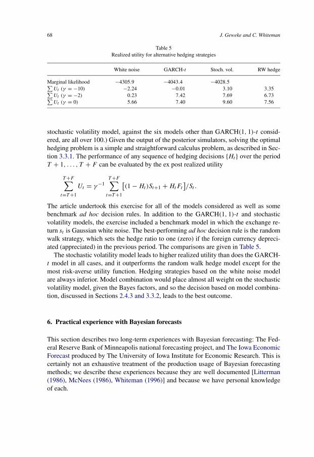
68 J. Geweke and C. Whiteman
Table 5Realized utility for alternative hedging strategies
White noise GARCH-t Stoch. vol. RW hedge
Marginal likelihood −4305.9 −4043.4 −4028.5∑Ut (γ = −10) −2.24 −0.01 3.10 3.35∑Ut (γ = −2) 0.23 7.42 7.69 6.73∑Ut (γ = 0) 5.66 7.40 9.60 7.56
stochastic volatility model, against the six models other than GARCH(1, 1)-t consid-ered, are all over 100.) Given the output of the posterior simulators, solving the optimalhedging problem is a simple and straightforward calculus problem, as described in Sec-tion 3.3.1. The performance of any sequence of hedging decisions {Ht } over the periodT + 1, . . . , T + F can be evaluated by the ex post realized utility
T +F∑t=T +1
Ut = γ −1T +F∑
t=T +1
[(1 − Ht)St+1 + HtFt
]/St .
The article undertook this exercise for all of the models considered as well as somebenchmark ad hoc decision rules. In addition to the GARCH(1, 1)-t and stochasticvolatility models, the exercise included a benchmark model in which the exchange re-turn st is Gaussian white noise. The best-performing ad hoc decision rule is the randomwalk strategy, which sets the hedge ratio to one (zero) if the foreign currency depreci-ated (appreciated) in the previous period. The comparisons are given in Table 5.
The stochastic volatility model leads to higher realized utility than does the GARCH-t model in all cases, and it outperforms the random walk hedge model except for themost risk-averse utility function. Hedging strategies based on the white noise modelare always inferior. Model combination would place almost all weight on the stochasticvolatility model, given the Bayes factors, and so the decision based on model combina-tion, discussed in Sections 2.4.3 and 3.3.2, leads to the best outcome.
6. Practical experience with Bayesian forecasts
This section describes two long-term experiences with Bayesian forecasting: The Fed-eral Reserve Bank of Minneapolis national forecasting project, and The Iowa EconomicForecast produced by The University of Iowa Institute for Economic Research. This iscertainly not an exhaustive treatment of the production usage of Bayesian forecastingmethods; we describe these experiences because they are well documented [Litterman(1986), McNees (1986), Whiteman (1996)] and because we have personal knowledgeof each.
Ch. 1: Bayesian Forecasting 69
6.1. National BVAR forecasts: The Federal Reserve Bank of Minneapolis
Litterman’s thesis work at the University of Minnesota (“the U”) was coincident with hisemployment as a research assistant in the Research Department at the Federal ReserveBank of Minneapolis (the “Bank”). In 1978 and 1979, he wrote a computer program,“Predict” to carry out the calculations described in Section 4. At the same time, ThomasDoan, also a graduate student at the U and likewise a research assistant at the Bank, waswriting code to carry out regression, ARIMA, and other calculations for staff econo-mists. Thomas Turner, a staff economist at the Bank, had modified a program writtenby Christopher Sims, “Spectre”, to incorporate regression calculations using complexarithmetic to facilitate frequency-domain treatment of serial correlation. By the sum-mer of 1979, Doan had collected his own routines in a flexible shell and incorporated thefeatures of Spectre and Predict (in most cases completely recoding their routines) to pro-duce the program RATS (for “Regression Analysis of Time Series”). Indeed, Litterman(1979) indicates that some of the calculations for his paper were carried out in RATS.The program subsequently became a successful Doan-Litterman commercial venture,and did much to facilitate the adoption of BVAR methods throughout academics andbusiness.
It was in fact Litterman himself who was responsible for the Bank’s focus on BVARforecasts. He had left Minnesota in 1979 to take a position as Assistant Professor ofEconomics at M.I.T., but was hired back to the Bank two years later. Based on workcarried out while a graduate student and subsequently at M.I.T., in 1980 Litterman beganissuing monthly forecasts using a six-variable BVAR of the type described in Section 4.The six variables were: real GNP, the GNP price deflator, real business fixed investment,the 3-month Treasury bill rate, the unemployment rate, and the money supply (M1).Upon his return to the Bank, the BVAR for these variables [described in Litterman(1986)] became known as the “Minneapolis Fed model”.
In his description of five years of monthly experience forecasting with the BVARmodel, Litterman (1986) notes that unlike his competition at the time – large, expensivecommercial forecasts produced by the likes of Data Resources Inc. (DRI), WhartonEconometric Forecasting Associates (WEFA), and Chase – his forecasts were producedmechanically, without judgemental adjustment. The BVAR often produced forecastsvery different from the commercial predictions, and Litterman notes that they weresometimes regarded by recipients (Litterman’s mailing list of academics, which in-cluded both of us) as too “volatile” or “wild”. Still, his procedure produced real timeforecasts that were “at least competitive with the best forecasts commercially avail-able” [Litterman (1986, p. 35)]. McNees’s (1986) independent assessment, which alsoinvolved comparisons with an even broader collection of competitors was that Litter-man’s BVAR was “generally the most accurate or among the most accurate” for realGNP, the unemployment rate, and investment. The BVAR price forecasts, on the otherhand, were among the least accurate.
Subsequent study by Litterman resulted in the addition of an exchange rate measureand stock prices that improved, at least experimentally, the performance of the model’s
70 J. Geweke and C. Whiteman
price predictions. Other models were developed as well; Litterman (1984) describesa 46-variable monthly national forecasting model, while Amirizadeh and Todd (1984)describe a five-state model of the 9th Federal Reserve District (that of the MinneapolisFed) involving 3 or 4 equations per state. Moreover, the models were used regularly inBank discussions, and reports based on them appeared regularly in the Minneapolis FedQuarterly Review [e.g., Litterman (1984), Litterman (1985)].
In 1986, Litterman left the Bank to go to Goldman–Sachs. This required dissolutionof the Doan–Litterman joint venture, and Doan subsequently formed Estima, Inc. tofurther develop and market RATS. It also meant that forecast production fell to staffeconomists whose research interests were not necessarily focused on the further devel-opment of BVARs [e.g., Roberds and Todd (1987), Runkle (1988), Miller and Runkle(1989), Runkle (1989, 1990, 1991)]. This, together with the pain associated with ex-plaining the inevitable forecast errors, caused enthusiasm for the BVAR effort at theBank to wane over the ensuing half dozen years, and the last Quarterly Review “out-look” article based on a BVAR forecast appeared in 1992 [Runkle (1992)]. By the springof 1993, the Bank’s BVAR efforts were being overseen by a research assistant (albeit aquite capable one), and the authors of this paper were consulted by the leadership of theBank’s Research Department regarding what steps were required to ensure academiccurrency and reliability of the forecasting effort. The cost – our advice was to employ astaff economist whose research would be complementary to the production of forecasts– was regarded as too high given the configuration of economists in the department, anddevelopment of the forecasting model and procedures at the Bank effectively ceased.
Cutting-edge development of Bayesian forecasting models reappeared relatively soonwithin the Federal Reserve System. In 1995, Tao Zha, who had written a Minnesota the-sis under the direction of Chris Sims, moved from the University of Saskatchewan tothe Federal Reserve Bank of Atlanta, and began implementing the developments de-scribed in Sims and Zha (1998, 1999) to produce regular forecasts for internal briefingpurposes. These efforts, which utilize the over-identified procedures described in Sec-tion 4.4, are described in Robertson and Tallman (1999a, 1999b) and Zha (1998), butthere is no continuous public record of forecasts comparable to Litterman’s “Five Yearsof Experience”.
6.2. Regional BVAR forecasts: economic conditions in Iowa
In 1990, Whiteman became Director of the Institute for Economic Research at the Uni-versity of Iowa. Previously, the Institute had published forecasts of general economicconditions and had produced tax revenue forecasts for internal use of the state’s De-partment of Management by judgmentally adjusting the product of a large commercialforecaster. These forecasts had not been especially accurate and were costing the statetens of thousands of dollars each year. As a consequence, an “Iowa Economic Forecast”model was constructed based on BVAR technology, and forecasts using it have beenissued continuously each quarter since March 1990.
Ch. 1: Bayesian Forecasting 71
The Iowa model consists of four linked VARs. Three of these involve income, realincome, and employment, and are treated using mixed estimation and the priors out-lined in Litterman (1979) and Doan, Litterman and Sims (1984). The fourth VAR, forpredicting aggregate state tax revenue, is much smaller, and fully Bayesian predictivedensities are produced from it under a diffuse prior.
The income and employment VARs involve variables that were of interest to the IowaForecasting Council, a group of academic and business economists that met quarterly toadvise the Governor on economic conditions. The nominal income VAR includes totalnonfarm income and four of its components: wage and salary disbursements, propertyincome, transfers, and farm income. These five variables together with their nationalanalogues, four lags of each, and a constant and seasonal dummy variables complete thespecification of the model for the observables. The prior is Litterman’s (1979) (recallspecifications (61) and (62), with a generalization of the “other’s weight” that embodiesthe notion that national variables are much more likely to be helpful in predicting Iowavariables than the converse. Details can be found in Whiteman (1996) and Otrok andWhiteman (1998). The real income VAR is constructed in parallel fashion after deflatingeach income variable by the GDP deflator.
The employment VAR is constructed similarly, using aggregate Iowa employment(nonfarm employment) together with the state’s population and five components of em-ployment: durable and nondurable goods manufacturing employment, and employmentin services and wholesale and retail trade. National analogues of each are used for atotal of 14 equations. Monthly data available from the U.S. Bureau of Labor Statisticsand Iowa’s Department of Workforce Development are aggregated to a quarterly basis.As in the income VAR, four lags, a constant, and seasonal dummies are included. Theprior is very similar to the one employed in the income VARs.
The revenue VAR incorporates two variables: total personal income and total taxreceipts (on a cash basis.) The small size was dictated by data availability at the timeof the initial model construction: only seven years’ of revenue data were available on aconsistent accounting standard as of the beginning of 1990. Monthly data are aggregatedto a quarterly basis; other variables include a constant and seasonal dummies. Until1997, two lags were used; thereafter, four were employed. The prior is diffuse, as in (66).
Each quarter, the income and employment VARs are “estimated” (via mixed estima-tion), and [as in Litterman (1979) and Doan, Litterman and Sims (1984)] parameterestimates so obtained are used to produce forecasts using the chain rule of forecast-ing for horizons of 12 quarters. Measures of uncertainty at each horizon are calculatedeach quarter from a pseudo-real time forecasting experiment [recall the description ofLitterman’s (1979) experiment] over the 40 quarters immediately prior to the end ofthe sample. Forecasts and uncertainty measures are published in the “Iowa EconomicForecast”.
Production of the revenue forecasts involves normal-Wishart sampling. In particular,each quarter, the Wishart distribution is sampled repeatedly for innovation covariancematrices; using each such sampled covariance matrix, a conditionally Gaussian para-meter vector and a sequence of Gaussian errors is drawn and used to seed a dynamic
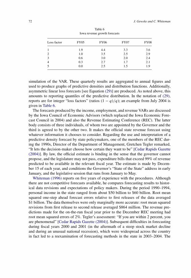
72 J. Geweke and C. Whiteman
Table 6Iowa revenue growth forecasts
Loss factor FY05 FY06 FY07 FY08
1 1.9 4.4 3.3 3.62 1.0 3.5 2.5 2.93 0.6 3.0 2.0 2.44 0.3 2.7 1.7 2.15 0.0 2.5 1.5 1.9
simulation of the VAR. These quarterly results are aggregated to annual figures andused to produce graphs of predictive densities and distribution functions. Additionally,asymmetric linear loss forecasts [see Equation (29)] are produced. As noted above, thisamounts to reporting quantiles of the predictive distribution. In the notation of (29),reports are for integer “loss factors” (ratios (1 − q)/q); an example from July 2004 isgiven in Table 6.
The forecasts produced by the income, employment, and revenue VARs are discussedby the Iowa Council of Economic Advisors (which replaced the Iowa Economic Fore-cast Council in 2004) and also the Revenue Estimating Conference (REC). The latterbody consists of three individuals, of whom two are appointed by the Governor and thethird is agreed to by the other two. It makes the official state revenue forecast usingwhatever information it chooses to consider. Regarding the use and interpretation of apredictive density forecast by state policymakers, one of the members of the REC dur-ing the 1990s, Director of the Department of Management, Gretchen Tegler remarked,“It lets the decision-maker choose how certain they want to be” [Cedar Rapids Gazette(2004)]. By law, the official estimate is binding in the sense that the governor cannotpropose, and the legislature may not pass, expenditure bills that exceed 99% of revenuepredicted to be available in the relevant fiscal year. The estimate is made by Decem-ber 15 of each year, and conditions the Governor’s “State of the State” address in earlyJanuary, and the legislative session that runs from January to May.
Whiteman (1996) reports on five years of experience with the procedures. Althoughthere are not competitive forecasts available, he compares forecasting results to histor-ical data revisions and expectations of policy makers. During the period 1990–1994,personal income in the state ranged from about $50 billion to $60 billion. Root meansquared one-step ahead forecast errors relative to first releases of the data averaged$1 billion. The data themselves were only marginally more accurate: root mean squaredrevisions from first release to second release averaged $864 million. The revenue pre-dictions made for the on-the-run fiscal year prior to the December REC meeting hadroot mean squared errors of 2%. Tegler’s assessment: “If you are within 2 percent, youare phenomenal” [Cedar Rapids Gazette (2004)]. Subsequent difficulties in forecastingduring fiscal years 2000 and 2001 (in the aftermath of a steep stock market declineand during an unusual national recession), which were widespread across the countryin fact led to a reexamination of forecasting methods in the state in 2003–2004. The
Ch. 1: Bayesian Forecasting 73
outcome of this was a reaffirmation of official faith in the approach, perhaps reflectingformer State Comptroller Marvin Seldon’s comment at the inception of BVAR use inIowa revenue forecasting: “If you can find a revenue forecaster who can get you within3 percent, keep him” [Seldon (1990)].
References
Aguilar, O., West, M. (2000). “Bayesian dynamic factor models and portfolio allocation”. Journal of Businessand Economic Statistics 18, 338–357.
Albert, J.H., Chib, S. (1993). “Bayes inference via Gibbs sampling of autoregressive time-series subject toMarkov mean and variance shifts”. Journal of Business and Economic Statistics 11, 1–15.
Amirizadeh, H., Todd, R. (1984). “More growth ahead for ninth district states”. Federal Reserve Bank ofMinneapolis Quarterly Review 4, 8–17.
Amisano, G., Serati, M. (1999). “Forecasting cointegrated series with BVAR models”. Journal of Forecast-ing 18, 463–476.
Barnard, G.A. (1963). “New methods of quality control”. Journal of the Royal Statistical Society Series A 126,255–259.
Barndorff-Nielsen, O.E., Schou, G. (1973). “On the reparameterization of autoregressive models by partialautocorrelations”. Journal of Multivariate Analysis 3, 408–419.
Barnett, G., Kohn, R., Sheather, S. (1996). “Bayesian estimation of an autoregressive model using Markovchain Monte Carlo”. Journal of Econometrics 74, 237–254.
Bates, J.M., Granger, C.W.J. (1969). “The combination of forecasts”. Operations Research 20, 451–468.Bayarri, M.J., Berger, J.O. (1998). “Quantifying surprise in the data and model verification”. In: Berger, J.O.,
Bernardo, J.M., Dawid, A.P., Lindley, D.V., Smith, A.F.M. (Eds.), Bayesian Statistics, vol. 6. OxfordUniversity Press, Oxford, pp. 53–82.
Berger, J.O., Delampady, M. (1987). “Testing precise hypotheses”. Statistical Science 2, 317–352.Bernardo, J.M., Smith, A.F.M. (1994). Bayesian Theory. Wiley, New York.Bos, C.S., Mahieu, R.J., van Dijk, H.K. (2000). “Daily exchange rate behaviour and hedging of currency
risk”. Journal of Applied Econometrics 15, 671–696.Box, G.E.P. (1980). “Sampling and Bayes inference in scientific modeling and robustness”. Journal of the
Royal Statistical Society Series A 143, 383–430.Box, G.E.P., Jenkins, G.M. (1976). Time Series Analysis, Forecasting and Control. Holden-Day, San Fran-
cisco.Brav, A. (2000). “Inference in long-horizon event studies: A Bayesian approach with application to initial
public offerings”. The Journal of Finance 55, 1979–2016.Carter, C.K., Kohn, R. (1994). “On Gibbs sampling for state-space models”. Biometrika 81, 541–553.Carter, C.K., Kohn, R. (1996). “Markov chain Monte Carlo in conditionally Gaussian state space models”.
Biometrika 83, 589–601.Cedar Rapids Gazette. (2004). “Rain or shine? Professor forecasts funding,” Sunday, February 1.Chatfield, C. (1976). “Discussion on the paper by Professor Harrison and Mr. Stevens”. Journal of the Royal
Statistical Society. Series B (Methodological) 38 (3), 231–232.Chatfield, C. (1993). “Calculating interval forecasts”. Journal of Business and Economic Statistics 11, 121–
135.Chatfield, C. (1995). “Model uncertainty, data mining, and statistical inference”. Journal of the Royal Statis-
tical Society Series A 158, 419–468.Chib, S. (1995). “Marginal likelihood from the Gibbs output”. Journal of the American Statistical Associa-
tion 90, 1313–1321.Chib, S. (1996). “Calculating posterior distributions and modal estimates in Markov mixture models”. Journal
of Econometrics 75, 79–97.
74 J. Geweke and C. Whiteman
Chib, S., Greenberg, E. (1994). “Bayes inference in regression models with ARMA(p, q) errors”. Journal ofEconometrics 64, 183–206.
Chib, S., Greenberg, E. (1995). “Understanding the Metropolis–Hastings algorithm”. The American Statisti-cian 49, 327–335.
Chib, S., Jeliazkov, J. (2001). “Marginal likelihood from the Metropolis–Hastings output”. Journal of theAmerican Statistical Association 96, 270–281.
Christoffersen, P.F. (1998). “Evaluating interval forecasts”. International Economic Review 39, 841–862.Chulani, S., Boehm, B., Steece, B. (1999). “Bayesian analysis of empirical software engineering cost models”.
IEEE Transactions on Software Engineering 25, 573–583.Clemen, R.T. (1989). “Combining forecasts – a review and annotated bibliography”. International Journal of
Forecasting 5, 559–583.Cogley, T., Morozov, S., Sargent, T. (2005). “Bayesian fan charts for U.K. inflation: Forecasting and sources
of uncertainty in an evolving monetary system,” Journal of Economic Dynamics and Control, in press.Dawid, A.P. (1984). “Statistical theory: The prequential approach”. Journal of the Royal Statistical Society
Series A 147, 278–292.DeJong, D.N., Ingram, B.F., Whiteman, C.H. (2000). “A Bayesian approach to dynamic macroeconomics”.
Journal of Econometrics 98, 203–223.DeJong, P., Shephard, N. (1995). “The simulation smoother for time series models”. Biometrika 82, 339–350.Diebold, F.X. (1998). Elements of Forecasting. South-Western College Publishing, Cincinnati.Doan, T., Litterman, R.B., Sims, C.A. (1984). “Forecasting and conditional projection using realistic prior
distributions”. Econometric Reviews 3, 1–100.Draper, D. (1995). “Assessment and propagation of model uncertainty”. Journal of the Royal Statistical Soci-
ety Series B 57, 45–97.Drèze, J.H. (1977). “Bayesian regression analysis using poly-t densities”. Journal of Econometrics 6, 329–
354.Drèze, J.H., Morales, J.A. (1976). “Bayesian full information analysis of simultaneous equations”. Journal of
the American Statistical Association 71, 919–923.Drèze, J.H., Richard, J.F. (1983). “Bayesian analysis of simultaneous equation systems”. In: Griliches, Z.,
Intrilligator, M.D. (Eds.), Handbook of Econometrics, vol. I. North-Holland, Amsterdam, pp. 517–598.Edwards, W., Lindman, H., Savage, L.J. (1963). “Bayesian statistical inference for psychological research”.
Psychological Review 70, 193–242.Engle, R.F., Yoo, B.S. (1987). “Forecasting and testing in cointegrated systems”. Journal of Econometrics 35,
143–159.Fair, R.C. (1980). “Estimating the expected predictive accuracy of econometric models”. International Eco-
nomic Review 21, 355–378.Fruhwirth-Schnatter, S. (1994). “Data augmentation and dynamic linear models”. Journal of Time Series
Analysis 15, 183–202.Garcia-Ferer, A., Highfield, R.A., Palm, F., Zellner, A. (1987). “Macroeconomic forecasting using pooled
international data”. Journal of Business and Economic Statistics 5, 53–67.Geisel, M.S. (1975). “Bayesian comparison of simple macroeconomic models”. In: Fienberg, S.E., Zellner, A.
(Eds.), Studies in Bayesian Econometrics and Statistics: In Honor of Leonard J. Savage. North-Holland,Amsterdam, pp. 227–256.
Geisser, S. (1993). Predictive Inference: An Introduction. Chapman and Hall, London.Gelfand, A.E., Dey, D.K. (1994). “Bayesian model choice: Asymptotics and exact calculations”. Journal of
the Royal Statistical Society Series B 56, 501–514.Gelfand, A.E., Smith, A.F.M. (1990). “Sampling based approaches to calculating marginal densities”. Journal
of the American Statistical Association 85, 398–409.Gelman, A. (2003). “A Bayesian formulation of exploratory data analysis and goodness-of-fit testing”. Inter-
national Statistical Review 71, 369–382.Gelman, A., Carlin, J.B., Stern, H.S., Rubin, D.B. (1995). Bayesian Data Analysis. Chapman and Hall, Lon-
don.
Ch. 1: Bayesian Forecasting 75
Geman, S., Geman, D. (1984). “Stochastic relaxation, Gibbs distributions and the Bayesian restoration ofimages”. IEEE Transactions on Pattern Analysis and Machine Intelligence 6, 721–741.
George, E., McCulloch, R.E. (1993). “Variable selection via Gibbs sampling”. Journal of the American Sta-tistical Association 99, 881–889.
Gerlach, R., Carter, C., Kohn, R. (2000). “Efficient Bayesian inference for dynamic mixture models”. Journalof the American Statistical Association 95, 819–828.
Geweke, J. (1988). “Antithetic acceleration of Monte Carlo integration in Bayesian inference”. Journal ofEconometrics 38, 73–90.
Geweke, J. (1989a). “Bayesian inference in econometric models using Monte Carlo integration”. Economet-rica 57, 1317–1340.
Geweke, J. (1989b). “Exact predictive densities in linear models with ARCH disturbances”. Journal of Econo-metrics 40, 63–86.
Geweke, J. (1991). “Generic, algorithmic approaches to Monte Carlo integration in Bayesian inference”.Contemporary Mathematics 115, 117–135.
Geweke, J. (1993). “Bayesian treatment of the independent Student-t linear model”. Journal of AppliedEconometrics 8, S19–S40.
Geweke, J. (1996a). “Monte Carlo simulation and numerical integration”. In: Amman, H., Kendrick, D., Rust,J. (Eds.), Handbook of Computational Economics. North-Holland, Amsterdam, pp. 731–800.
Geweke, J. (1996b). “Variable selection and model comparison in regression”. In: Berger, J.O., Bernardo,J.M., Dawid, A.P., Smith, A.F.M. (Eds.), Bayesian Statistics, vol. 5. Oxford University Press, Oxford,pp. 609–620.
Geweke, J. (1998). “Simulation methods for model criticism and robustness analysis”. In: Berger, J.O.,Bernardo, J.M., Dawid, A.P., Smith, A.F.M. (Eds.), Bayesian Statistics, vol. 6. Oxford University Press,Oxford, pp. 275–299.
Geweke, J. (1999). “Using simulation methods for Bayesian econometric models: Inference, developmentand communication”. Econometric Reviews 18, 1–126.
Geweke, J. (2000). “Bayesian communication: The BACC system”. In: 2000 Proceedings of the Section onBayesian Statistical Sciences of the American Statistical Association, pp. 40–49.
Geweke, J. (2005). Contemporary Bayesian Econometrics and Statistics. Wiley, New York.Geweke, J., McCausland, W. (2001). “Bayesian specification analysis in econometrics”. American Journal of
Agricultural Economics 83, 1181–1186.Geweke, J., Zhou, G. (1996). “Measuring the pricing error of the arbitrage pricing theory”. The Review of
Financial Studies 9, 557–587.Gilks, W.R., Richardson, S., Spiegelhaldter, D.J. (1996). Markov Chain Monte Carlo in Practice. Chapman
and Hall, London.Good, I.J. (1956). “The surprise index for the multivariate normal distribution”. Annals of Mathematical
Statistics 27, 1130–1135.Granger, C.W.J. (1986). “Comment” (on McNees, 1986). Journal of Business and Economic Statistics 4,
16–17.Granger, C.W.J. (1989). “Invited review: Combining forecasts – twenty years later”. Journal of Forecasting 8,
167–173.Granger, C.W.J., Joyeux, R. (1980). “An introduction to long memory time series models and fractional
differencing”. Journal of Time Series Analysis 1, 15–29.Granger, C.W.J., Ramanathan, R. (1984). “Improved methods of combining forecasts”. Journal of Forecast-
ing 3, 197–204.Greene, W.H. (2003). Econometric Analysis, fifth ed. Prentice-Hall, Upper Saddle River, NJ.Hammersly, J.M., Handscomb, D.C. (1964). Monte Carlo Methods. Methuen and Company, London.Hammersly, J.M., Morton, K.H. (1956). “A new Monte Carlo technique: Antithetic variates”. Proceedings of
the Cambridge Philosophical Society 52, 449–474.Harrison, P.J., Stevens, C.F. (1976). “Bayesian forecasting”. Journal of the Royal Statistical Society Series B
(Methodological) 38 (3), 205–247.
76 J. Geweke and C. Whiteman
Haslett, J., Raftery, A.E. (1989). “Space-time modeling with long-memory dependence: Assessing Ireland’swind power resource”. Applied Statistics 38, 1–50.
Hastings, W.K. (1970). “Monte Carlo sampling methods using Markov chains and their applications”. Bio-metrika 57, 97–109.
Heckerman, D. (1997). “Bayesian networks for data mining”. Data Mining and Knowledge Discovery 1,79–119.
Hildreth, C. (1963). “Bayesian statisticians and remote clients”. Econometrica 31, 422–438.Hoerl, A.E., Kennard, R.W. (1970). “Ridge regression: Biased estimation for nonorthogonal problems”. Tech-
nometrics 12, 55–67.Hoeting, J.A., Madigan, D., Raftery, A.E., Volinsky, C.T. (1999). “Bayesian model averaging: A tutorial”.
Statistical Science 14, 382–401.Hosking, J.R.M. (1981). “Fractional differencing”. Biometrika 68, 165–176.Huerta, G., West, M. (1999). “Priors and component structures in autoregressive time series models”. Journal
of the Royal Statistical Society Series B 61, 881–899.Hull, J., White, A. (1987). “The pricing of options on assets with stochastic volatilities”. Journal of Finance 42,
281–300.Ingram, B.F., Whiteman, C.H. (1994). “Supplanting the Minnesota prior – forecasting macroeconomic time
series using real business-cycle model priors”. Journal of Monetary Economics 34, 497–510.Iowa Economic Forecast, produced quarterly by the Institute for Economic Research in the Tippie College of
Business at The University of Iowa. Available at www.biz.uiowa.edu/econ/econinst.Jacquier, C., Polson, N.G., Rossi, P.E. (1994). “Bayesian analysis of stochastic volatility models”. Journal of
Business and Economic Statistics 12, 371–389.James, W., Stein, C. (1961). “Estimation with quadratic loss”. In: Proceedings of the Fourth Berkeley Sympo-
sium on Mathematical Statistics and Probability. University of California Press, Berkeley, pp. 361–379.Jeffreys, H. (1939). Theory of Probability. Clarendon Press, Oxford.Johansen, S. (1988). “Statistical analysis of cointegration vectors”. Journal of Economic Dynamics and Con-
trol 12, 231–254.Kadiyala, K.R., Karlsson, S. (1993). “Forecasting with generalized Bayesian vector autoregressions”. Journal
of Forecasting 12, 365–378.Kadiyala, K.R., Karlsson, S. (1997). “Numerical methods for estimation and inference in Bayesian VAR-
models”. Journal of Applied Econometrics 12, 99–132.Kass, R.E., Raftery, A.E. (1996). “Bayes factors”. Journal of the American Statistical Association 90, 773–
795.Kim, S., Shephard, N., Chib, S. (1998). “Stochastic volatility: Likelihood inference and comparison with
ARCH models”. Review of Economic Studies 64, 361–393.Kling, J.L. (1987). “Predicting the turning points of business and economic time series”. Journal of Busi-
ness 60, 201–238.Kling, J.L., Bessler, D.A. (1989). “Calibration-based predictive distributions: An application of prequential
analysis to interest rates, money, prices and output”. Journal of Business 62, 477–499.Kloek, T., van Dijk, H.K. (1978). “Bayesian estimates of equation system parameters: An application of
integration by Monte Carlo”. Econometrica 46, 1–20.Koop, G. (2001). “Bayesian inference in models based on equilibrium search theory”. Journal of Economet-
rics 102, 311–338.Koop, G. (2003). Bayesian Econometrics. Wiley, Chichester.Koop, G., Ley, E., Osiewalski, J., Steel, M.F.J. (1997). “Bayesian analysis of long memory and persistence
using ARFIMA models”. Journal of Econometrics 76, 149–169.Lancaster, T. (2004). An Introduction to Modern Bayesian Econometrics. Blackwell, Malden, MA.Leamer, E.E. (1972). “A class of informative priors and distributed lag analysis”. Econometrica 40, 1059–
1081.Leamer, E.E. (1978). Specification Searches. Wiley, New York.Lesage, J.P. (1990). “A comparison of the forecasting ability of ECM and VAR models”. The Review of
Economics and Statistics 72, 664–671.
Ch. 1: Bayesian Forecasting 77
Lindley, D., Smith, A.F.M. (1972). “Bayes estimates for the linear model”. Journal of the Royal StatisticalSociety Series B 34, 1–41.
Litterman, R.B. (1979). “Techniques of forecasting using vector autoregressions”. Working Paper 115, Fed-eral Reserve Bank of Minneapolis.
Litterman, R.B. (1980). “A Bayesian procedure for forecasting with vector autoregressions”. Working Paper,Massachusetts Institute of Technology.
Litterman, R.B. (1984). “Above average national growth in 1985 and 1986”. Federal Reserve Bank of Min-neapolis Quarterly Review.
Litterman, R.B. (1985). “How monetary policy in 1985 affects the outlook”. Federal Reserve Bank of Min-neapolis Quarterly Review.
Litterman, R.B. (1986). “Forecasting with Bayesian vector autoregressions – 5 years of experience”. Journalof Business and Economic Statistics 4, 25–38.
Maddala, G.S. (1977). Econometrics. McGraw-Hill, New York.Marriott, J., Ravishanker, N., Gelfand, A., Pai, J. (1996). “Bayesian analysis of ARMA processes: Complete
sampling-based inference under exact likelihoods”. In: Barry, D.A., Chaloner, K.M., Geweke, J. (Eds.),Bayesian Analysis in Econometrics and Statistics: Essays in Honor of Arnold Zellner. Wiley, New York,pp. 243–256.
McNees, S.K. (1975). “An evaluation of economic forecasts”. New England Economic Review, 3–39.McNees, S.K. (1986). “Forecasting accuracy of alternative techniques: A comparison of U.S. macroeconomic
forecasts”. Journal of Business and Economic Statistics 4, 5–15.Melino, A., Turnbull, S. (1990). “Pricing foreign currency options with stochastic volatility”. Journal of
Econometrics 45, 7–39.Meng, X.L. (1994). “Posterior predictive p-values”. Annals of Statistics 22, 1142–1160.Meng, X.L., Wong, W.H. (1996). “Simulating ratios of normalizing constants via a simple identity: A theo-
retical exploration”. Statistica Sinica 6, 831–860.Metropolis, N., Rosenbluth, A.W., Rosenbluth, M.N., Teller, A.H., Teller, E. (1953). “Equation of state cal-
culations by fast computing machines”. The Journal of Chemical Physics 21, 1087–1092.Miller, P.J., Runkle, D.E. (1989). “The U.S. economy in 1989 and 1990: Walking a fine line”. Federal Reserve
Bank of Minneapolis Quarterly Review.Min, C.K., Zellner, A. (1993). “Bayesian and non-Bayesian methods for combining models and forecasts
with applications to forecasting international growth rates”. Journal of Econometrics 56, 89–118.Monahan, J.F. (1983). “Fully Bayesian analysis of ARMA time series models”. Journal of Econometrics 21,
307–331.Monahan, J.F. (1984). “A note on enforcing stationarity in autoregressive moving average models”. Bio-
metrika 71, 403–404.Newbold, P. (1974). “The exact likelihood for a mixed autoregressive moving average process”. Bio-
metrika 61, 423–426.Otrok, C., Whiteman, C.H. (1998). “What to do when the crystal ball is cloudy: Conditional and unconditional
forecasting in Iowa”. Proceedings of the National Tax Association, 326–334.Pai, J.S., Ravishanker, N. (1996). “Bayesian modelling of ARFIMA processes by Markov chain Monte Carlo
methods”. Journal of Forecasting 15, 63–82.Palm, F.C., Zellner, A. (1992). “To combine or not to combine – Issues of combining forecasts”. Journal of
Forecasting 11, 687–701.Peskun, P.H. (1973). “Optimum Monte-Carlo sampling using Markov chains”. Biometrika 60, 607–612.Petridis, V., Kehagias, A., Petrou, L., Bakirtzis, A., Kiartzis, S., Panagiotou, H., Maslaris, N. (2001).
“A Bayesian multiple models combination method for time series prediction”. Journal of Intelligent andRobotic Systems 31, 69–89.
Plackett, R.L. (1950). “Some theorems in least squares”. Biometrica 37, 149–157.Pole, A., West, M., Harrison, J. (1994). Applied Bayesian Forecasting and Time Series Analysis. Chapman
and Hall, London.Porter-Hudak, S. (1982). “Long-term memory modelling – a simplified spectral approach”. Ph.D. thesis,
University of Wisconsin, Unpublished.
78 J. Geweke and C. Whiteman
RATS, computer program available from Estima, 1800 Sherman Ave., Suite 612, Evanston, IL 60201.Ravishanker, N., Ray, B.K. (1997a). “Bayesian analysis of vector ARMA models using Gibbs sampling”.
Journal of Forecasting 16, 177–194.Ravishanker, N., Ray, B.K. (1997b). “Bayesian analysis of vector ARFIMA process”. Australian Journal of
Statistics 39, 295–311.Ravishanker, N., Ray, B.K. (2002). “Bayesian prediction for vector ARFIMA processes”. International Jour-
nal of Forecasting 18, 207–214.Ripley, R.D. (1987). Stochastic Simulation. Wiley, New York.Roberds W., Todd R. (1987). “Forecasting and modelling the U.S. economy in 1986–1988”. Federal Reserve
Bank of Minneapolis Quarterly Review.Roberts, H.V. (1965). “Probabilistic prediction”. Journal of the American Statistical Association 60, 50–62.Robertson, J.C., Tallman, E.W. (1999a). “Vector autoregressions: Forecasting and reality”. Federal Reserve
Bank of Atlanta Economic Review 84 (First Quarter), 4–18.Robertson, J.C., Tallman, E.W. (1999b). “Improving forecasts of the Federal funds rate in a policy model”.
Journal of Business and Economic Statistics 19, 324–930.Robertson, J.C., Tallman, E.W., Whiteman, C.H. (2005). “Forecasting using relative entropy”. Journal of
Money, Credit, and Banking 37, 383–401.Rosenblatt, M. (1952). “Remarks on a multivariate transformation”. Annals of Mathematical Statistics 23,
470–472.Rothenberg, T.J. (1963). “A Bayesian analysis of simultaneous equation systems”. Report 6315, Econometric
Institute, Netherlands School of Economics, Rotterdam.Rubin, D.B. (1984). “Bayesianly justifiable and relevant frequency calculations for the applied statistician”.
Annals of Statistics 12, 1151–1172.Runkle, D.E. (1988). “Why no crunch from the crash?”. Federal Reserve Bank of Minneapolis Quarterly
Review.Runkle, D.E. (1989). “The U.S. economy in 1990 and 1991: Continued expansion likely”. Federal Reserve
Bank of Minneapolis Quarterly Review.Runkle, D.E. (1990). “Bad news from a forecasting model of the U.S. economy”. Federal Reserve Bank of
Minneapolis Quarterly Review.Runkle, D.E. (1991). “A bleak outlook for the U.S. economy”. Federal Reserve Bank of Minneapolis Quar-
terly Review.Runkle, D.E. (1992). “No relief in sight for the U.S. economy”. Federal Reserve Bank of Minneapolis Quar-
terly Review.Schotman, P., van Dijk, H.K. (1991). “A Bayesian analysis of the unit root in real exchange rates”. Journal of
Econometrics 49, 195–238.Seldon, M. (1990). Personal communication to Whiteman.Shao, J. (1989). “Monte Carlo approximations in Bayesian decision theory”. Journal of the American Statis-
tical Association 84, 727–732.Shephard, N., Pitt, M.K. (1997). “Likelihood analysis of non-Gaussian measurement time series”. Bio-
metrika 84, 653–667.Shiller, R.J. (1973). “A distributed lag estimator derived from smoothness priors”. Econometrica 41, 775–788.Shoesmith, G.L. (1995). “Multiple cointegrating vectors, error correction, and forecasting with Litterman’s
model”. International Journal of Forecasting 11, 557–567.Sims, C.A. (1974). “Distributed lags”. In: Intrilligator, M.D., Kendrick, P.A. (Eds.), Frontiers of Quantitative
Economics, vol. II. North-Holland, Amsterdam, pp. 239–332.Sims, C.A. (1980). “Macroeconomics and reality”. Econometrica 48, 1–48.Sims, C.A. (1992). “A nine-variable probabilistic macroeconomic forecasting model”. In: Stock, J.H., Watson,
M.W. (Eds.), Business Cycles, Indicators, and Forecasting. University of Chicago Press, Chicago.Sims, C.A., Zha, T.A. (1998). “Bayesian methods for dynamic multivariate models”. International Economic
Review 39, 949–968.Sims, C.A., Zha, T.A. (1999). “Error bands for impulse responses”. Econometrica 67, 1113–1155.
Ch. 1: Bayesian Forecasting 79
Smith, A.F.M. (1973). “A general Bayesian linear model”. Journal of the Royal Statistical Society Series B 35,67–75.
Smyth, D.J. (1983). “Short-run macroeconomic forecasting: The OECD performance”. Journal of Forecast-ing 2, 37–49.
Sowell, F. (1992a). “Maximum likelihood estimation of stationary univariate fractionally integrated models”.Journal of Econometrics 53, 165–188.
Sowell, F. (1992b). “Modeling long-run behavior with the fractional ARIMA model”. Journal of MonetaryEconomics 29, 277–302.
Stein, C.M. (1974). “Multiple regression”. In: Olkin, I. (Ed.), Contributions to Probability and Statistics:Essays in Honor of Harold Hotelling. Stanford University Press, Stanford.
Tanner, M.A., Wong, H.W. (1987). “The calculation of posterior distributions by data augmentation”. Journalof the American Statistical Association 82, 528–540.
Tauchen, G., Pitts, M. (1983). “The price–variability–volume relationship on speculative markets”. Econo-metrica 51, 485–505.
Tay, A.S., Wallis, K.F. (2000). “Density forecasting: A survey”. Journal of Forecasting 19, 235–254.Taylor, S. (1986). Modelling Financial Time Series. Wiley, New York.Theil, H. (1963). “On the use of incomplete prior information in regression analysis”. Journal of the American
Statistical Association 58, 401–414.Thompson, P.A. (1984). “Bayesian multiperiod prediction: Forecasting with graphics”. Ph.D. thesis, Univer-
sity of Wisconsin, Unpublished.Thompson, P.A., Miller, R.B. (1986). “Sampling the future: A Bayesian approach to forecasting from uni-
variate time series models”. Journal of Business and Economic Statistics 4, 427–436.Tierney, L. (1994). “Markov chains for exploring posterior distributions”. Annals of Statistics 22, 1701–1762.Tobias, J.L. (2001). “Forecasting output growth rates and median output growth rates: A hierarchical Bayesian
approach”. Journal of Forecasting 20, 297–314.Villani, M. (2001). “Bayesian prediction with cointegrated vector autoregressions”. International Journal of
Forecasting 17, 585–605.Waggoner, D.F., Zha, T. (1999). “Conditional forecasts in dynamic multivariate models”. Review of Eco-
nomics and Statistics 81, 639–651.Wecker, W. (1979). “Predicting the turning points of a time series”. Journal of Business 52, 35–50.Weiss, A.A. (1996). “Estimating time series models using the relevant cost function”. Journal of Applied
Econometrics 11, 539–560.West, M. (1995). “Bayesian inference in cyclical component dynamic linear models”. Journal of the American
Statistical Association 90, 1301–1312.West, M., Harrison, J. (1997). Bayesian Forecasting and Dynamic Models, second ed. Springer, New York.Whiteman, C.H. (1996). “Bayesian prediction under asymmetric linear loss: Forecasting state tax revenues in
Iowa”. In: Johnson, W.O., Lee, J.C., Zellner, A. (Eds.), Forecasting, Prediction and Modeling in Statisticsand Econometrics, Bayesian and non-Bayesian Approaches. Springer, New York.
Winkler, R.L. (1981). “Combining probability distributions from dependent information sources”. Manage-ment Science 27, 479–488.
Zellner, A. (1971). An Introduction to Bayesian Inference in Econometrics. Wiley, New York.Zellner, A. (1986). “Bayesian estimation and prediction using asymmetric loss functions”. Journal of the
American Statistical Association 81, 446–451.Zellner, A., Chen, B. (2001). “Bayesian modeling of economies and data requirements”. Macroeconomic
Dynamics 5, 673–700.Zellner, A., Hong, C. (1989). “Forecasting international growth rates using Bayesian shrinkage and other
procedures”. Journal of Econometrics 40, 183–202.Zellner, A., Hong, C., Gulati, G.M. (1990). “Turning points in economic time series, loss structures and
Bayesian forecasting”. In: Geisser, S., Hodges, J.S., Press, S.J., Zellner, A. (Eds.), Bayesian and Like-lihood Methods in Statistics and Econometrics: Essays in Honor of George A. Barnard. North-Holland,Amsterdam, pp. 371–393.

80 J. Geweke and C. Whiteman
Zellner, A., Hong, C., Min, C.K. (1991). “Bayesian exponentially weighted autoregression, time-varyingparameter, and pooling techniques”. Journal of Econometrics 49, 275–304.
Zellner, A., Min, C.K. (1995). “Gibbs sampler convergence criteria”. Journal of the American StatisticalAssociation 90, 921–927.
Zha, T.A. (1998). “A dynamic multivariate model for use in formulating policy”. Federal Reserve Bank ofAtlanta Economic Review 83 (First Quarter), 16–29.