Embed Size (px)
Citation preview

J. Daunizeau
Brain and Spine Institute, Paris, France
Wellcome Trust Centre for Neuroimaging, London, UK
Bayesian inference

Overview of the talk
1 Probabilistic modelling and representation of uncertainty
1.1 Bayesian paradigm
1.2 Hierarchical models
1.3 Frequentist versus Bayesian inference
2 Notes on Bayesian inference
2.1 Variational methods (ReML, EM, VB)
2.2 Family inference
2.3 Group-level model comparison
3 SPM applications
3.1 aMRI segmentation
3.2 Decoding of brain images
3.3 Model-based fMRI analysis (with spatial priors)
3.4 Dynamic causal modelling

Degree of plausibility desiderata:
- should be represented using real numbers (D1)
- should conform with intuition (D2)
- should be consistent (D3)
a=2 b=5
a=2
• normalization:
• marginalization:
• conditioning :
(Bayes rule)
Bayesian paradigm probability theory: basics
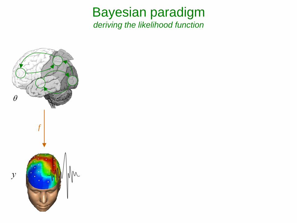
Bayesian paradigm deriving the likelihood function
- Model of data with unknown parameters:
y f e.g., GLM: f X
- But data is noisy: y f
- Assume noise/residuals is ‘small’:
2
2
1exp
2p
4 0.05P
→ Distribution of data, given fixed parameters:
2
2
1exp
2p y y f
f
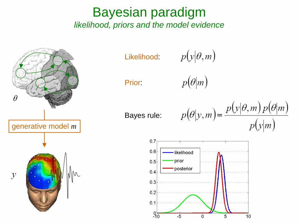
Likelihood:
Prior:
Bayes rule:
Bayesian paradigm likelihood, priors and the model evidence
generative model m

Bayesian paradigm forward and inverse problems
,p y m
forward problem
likelihood
,p y m
inverse problem
posterior distribution

Principle of parsimony :
« plurality should not be assumed without necessity »
y=f(
x)
y =
f(x
)
x
“Occam’s razor” :
mo
de
l evid
en
ce
p(y
|m)
space of all data sets
Model evidence:
Bayesian paradigm model comparison

••• inference
causality
Hierarchical models principle
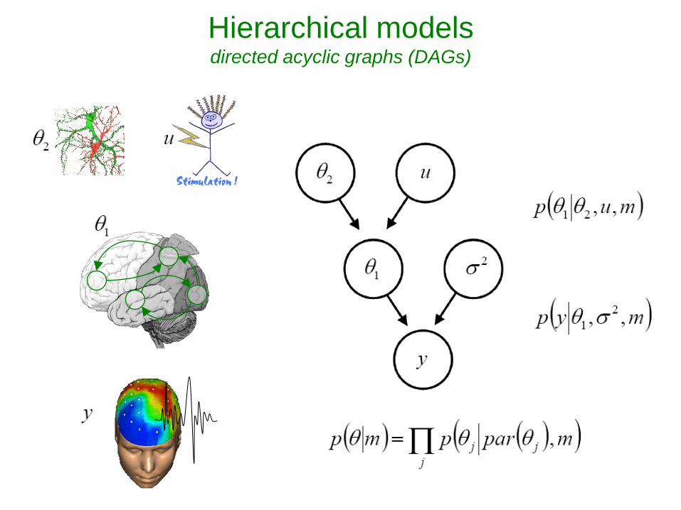
Hierarchical models directed acyclic graphs (DAGs)
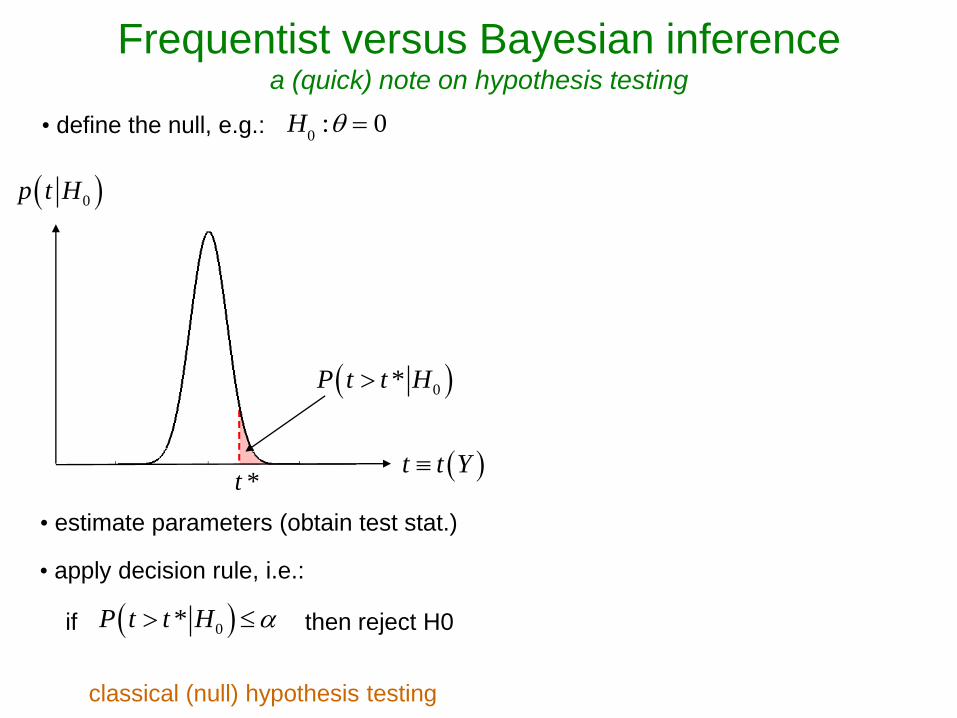
t t Y t *
0*P t t H
0p t H
0*P t t H if then reject H0
• estimate parameters (obtain test stat.)
H
0: 0• define the null, e.g.:
• apply decision rule, i.e.:
classical (null) hypothesis testing
• define two alternative models, e.g.:
• apply decision rule, e.g.:
Bayesian Model Comparison
Frequentist versus Bayesian inference a (quick) note on hypothesis testing
Y y
1p Y m
0p Y m
space of all datasets
if then accept m0
0
1
P m y
P m y
0 0
1 1
1 if 0:
0 otherwise
: 0,
m p m
m p m N

Overview of the talk
1 Probabilistic modelling and representation of uncertainty
1.1 Bayesian paradigm
1.2 Hierarchical models
1.3 Frequentist versus Bayesian inference
2 Notes on Bayesian inference
2.1 Variational methods (ReML, EM, VB)
2.2 Family inference
2.3 Group-level model comparison
3 SPM applications
3.1 aMRI segmentation
3.2 Decoding of brain images
3.3 Model-based fMRI analysis (with spatial priors)
3.4 Dynamic causal modelling

Variational methods VB / EM / ReML
→ VB : maximize the free energy F(q) w.r.t. the approximate posterior q(θ)
under some (e.g., mean field, Laplace) simplifying constraint
1 or 2q
1 or 2 ,p y m
1 2, ,p y m
1
2

Family-level inference trading inference resolution against statistical power
A B A B
A B
u
A B
u
P(m1|y) = 0.04 P(m2|y) = 0.25
P(m2|y) = 0.7 P(m2|y) = 0.01
1 1 max
0.3
mP e y P m y
model selection error risk:

Family-level inference trading inference resolution against statistical power
A B A B
A B
u
A B
u
P(m1|y) = 0.04 P(m2|y) = 0.25
P(m2|y) = 0.7 P(m2|y) = 0.01
1 1 max
0.3
mP e y P m y
model selection error risk:
P(f2|y) = 0.95 P(f1|y) = 0.05
1 1 max
0.05
fP e y P f y
family inference
(pool statistical evidence)
m f
P f y P m y

Group-level model comparison preliminary: Polya’s urn
1
0
i
i
m
m
→ ith marble is blue
→ ith marble is purple
→ (binomial) probability of drawing a set of n marbles:
1
1
1 ii
nmm
i
p m r r r
Thus, our belief about the proportion of blue marbles is:
1
1
11
11 ii
n p r nmm
i
ii
p r m p r r r E r m mn
r = proportion of blue marbles in the urn
r
1m 2m nm…

Group-level model comparison what if we are colour blind?
At least, we can measure how likely is the ith subject’s data under each model!
1
,n
i i i
i
p r m y p r p y m p m r
i ip y m n np y m 1 1p y m 2 2p y m
… …
r
1m 2m nm
ny2y1y
…
… ,
m
p r y p r m y
Our belief about the proportion of models is:
Exceedance probability: 'k k k kP r r y
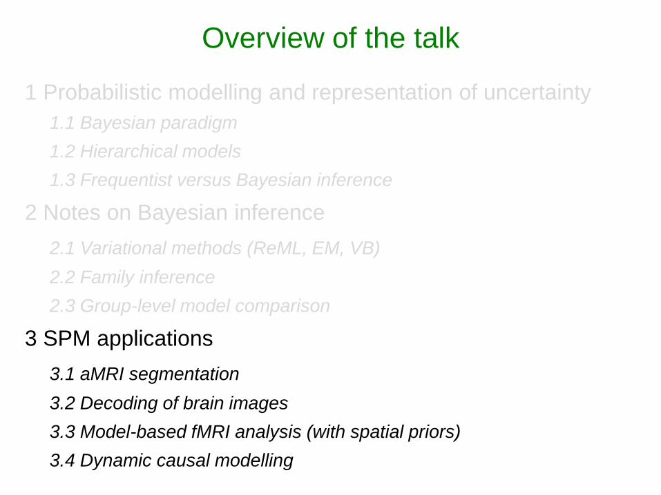
Overview of the talk
1 Probabilistic modelling and representation of uncertainty
1.1 Bayesian paradigm
1.2 Hierarchical models
1.3 Frequentist versus Bayesian inference
2 Notes on Bayesian inference
2.1 Variational methods (ReML, EM, VB)
2.2 Family inference
2.3 Group-level model comparison
3 SPM applications
3.1 aMRI segmentation
3.2 Decoding of brain images
3.3 Model-based fMRI analysis (with spatial priors)
3.4 Dynamic causal modelling

realignment smoothing
normalisation
general linear model
template
Gaussian
field theory
p <0.05
statistical
inference
segmentation
and normalisation
dynamic causal
modelling
posterior probability
maps (PPMs) multivariate
decoding
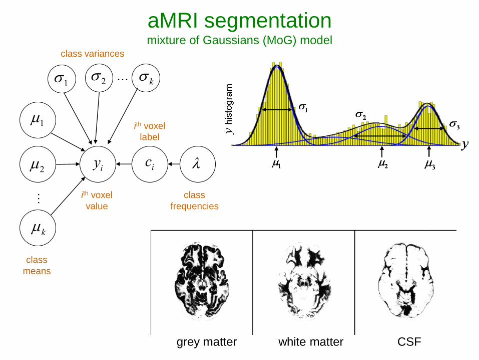
grey matter CSF white matter
…
…
yi ci
k
2
1
1 2 k
class variances
class
means
ith voxel
value
ith voxel
label
class
frequencies
aMRI segmentation mixture of Gaussians (MoG) model

Decoding of brain images recognizing brain states from fMRI
+
fixation cross
>>
pace response
log-evidence of X-Y sparse mappings:
effect of lateralization
log-evidence of X-Y bilateral mappings:
effect of spatial deployment

fMRI time series analysis spatial priors and model comparison
PPM: regions best explained
by short-term memory model
PPM: regions best explained
by long-term memory model
fMRI time series
GLM coeff
prior variance
of GLM coeff
prior variance
of data noise AR coeff
(correlated noise)
short-term memory
design matrix (X)
long-term memory
design matrix (X)

m2 m1 m3 m4
V1 V5 stim
PPC
attention
V1 V5 stim
PPC
attention
V1 V5 stim
PPC
attention
V1 V5 stim
PPC
attention
m1 m2 m3 m4
15
10
5
0
V1 V5 stim
PPC
attention
1.25
0.13
0.46
0.39
0.26
0.26
0.10 estimated
effective synaptic strengths
for best model (m4)
models marginal likelihood
ln p y m
Dynamic Causal Modelling network structure identification

I thank you for your attention.
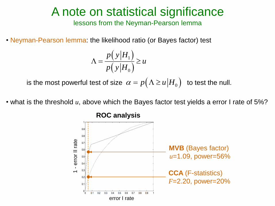
A note on statistical significance lessons from the Neyman-Pearson lemma
• Neyman-Pearson lemma: the likelihood ratio (or Bayes factor) test
1
0
p y Hu
p y H
is the most powerful test of size to test the null. 0p u H
MVB (Bayes factor)
u=1.09, power=56%
CCA (F-statistics)
F=2.20, power=20%
error I rate
1 -
err
or
II r
ate
ROC analysis
• what is the threshold u, above which the Bayes factor test yields a error I rate of 5%?