Embed Size (px)
Citation preview

Journal of Machine Learning Research 15 (2014) 1799-1847 Submitted 1/12; Revised 2/14; Published 5/14
Bayesian Inference with Posterior Regularizationand Applications to Infinite Latent SVMs
Jun Zhu [email protected] Chen [email protected] of Computer Science and TechnologyState Key Laboratory of Intelligent Technology and SystemsTsinghua National Laboratory for Information Science and TechnologyTsinghua UniversityBeijing, 100084 China
Eric P. Xing [email protected]
School of Computer Science
Carnegie Mellon University
Pittsburgh, PA 15213, USA
Editor: Tony Jebara
Abstract
Existing Bayesian models, especially nonparametric Bayesian methods, rely on speciallyconceived priors to incorporate domain knowledge for discovering improved latent represen-tations. While priors affect posterior distributions through Bayes’ rule, imposing posteriorregularization is arguably more direct and in some cases more natural and general. In thispaper, we present regularized Bayesian inference (RegBayes), a novel computational frame-work that performs posterior inference with a regularization term on the desired post-dataposterior distribution under an information theoretical formulation. RegBayes is more flex-ible than the procedure that elicits expert knowledge via priors, and it covers both directedBayesian networks and undirected Markov networks. When the regularization is inducedfrom a linear operator on the posterior distributions, such as the expectation operator, wepresent a general convex-analysis theorem to characterize the solution of RegBayes. Fur-thermore, we present two concrete examples of RegBayes, infinite latent support vector ma-chines (iLSVM) and multi-task infinite latent support vector machines (MT-iLSVM), whichexplore the large-margin idea in combination with a nonparametric Bayesian model for dis-covering predictive latent features for classification and multi-task learning, respectively.We present efficient inference methods and report empirical studies on several benchmarkdata sets, which appear to demonstrate the merits inherited from both large-margin learn-ing and Bayesian nonparametrics. Such results contribute to push forward the interfacebetween these two important subfields, which have been largely treated as isolated in thecommunity.
Keywords: Bayesian inference, posterior regularization, Bayesian nonparametrics,large-margin learning, classification, multi-task learning
1. Introduction
Over the past decade, nonparametric Bayesian models have gained remarkable popularity inmachine learning and other fields, partly owing to their desirable utility as a “nonparamet-
c©2014 Jun Zhu, Ning Chen and Eric P. Xing.

Zhu, Chen and Xing
ric” prior distribution for a wide variety of probabilistic models, thereby turning the largelyheuristic model selection practice, such as determining the unknown number of componentsin a mixture model (Antoniak, 1974) or the unknown dimensionality of latent features in afactor analysis model (Griffiths and Ghahramani, 2005), as a Bayesian inference problem inan unbounded model space. Popular examples include Gaussian process (GP) (Rasmussenand Ghahramani, 2002), Dirichlet process (DP) (Ferguson, 1973; Antoniak, 1974), and Betaprocess (BP) (Thibaux and Jordan, 2007). DP is often described with a Chinese restau-rant process (CRP) metaphor, and similarly BP is often described with an Indian buffetprocess (IBP) metaphor (Griffiths and Ghahramani, 2005). Such nonparametric Bayesianapproaches allow the model complexity to grow as more data are observed, which is a keyfactor differing them from other traditional “parametric” Bayesian models.
One recent development in practicing Bayesian nonparametrics is to relax some unreal-istic assumptions on data, such as homogeneity and exchangeability. For example, to handleheterogenous observations, predictor-dependent processes (MacEachern, 1999; Williamsonet al., 2010) have been proposed; and to relax the exchangeability assumption, stochasticprocesses with various correlation structures, such as hierarchical structures (Teh et al.,2006), temporal or spatial dependencies (Beal et al., 2002; Blei and Frazier, 2010), andstochastic ordering dependencies (Hoff, 2003; Dunson and Peddada, 2007), have been in-troduced. A common principle shared by these approaches is that they rely on defining,or in some unusual cases learning (Welling et al., 2012) a nonparametric Bayesian prior1
encoding some special structures, which indirectly2 influences the posterior distribution ofinterest through an interplay with a likelihood model according to the Bayes’ rule (alsoknown as Bayes’ theorem). In this paper, we explore a different principle known as poste-rior regularization, which offers an additional and arguably richer and more flexible set ofmeans to augment a posterior distribution under rich side information, such as predictivemargin, structural bias, etc., which can be harder, if possible, to be captured by a Bayesianprior.
Let Θ denote model parameters and H denote hidden variables. Then given a set ofobserved data D, posterior regularization (Ganchev et al., 2010) is generally defined assolving a regularized maximum likelihood estimation (MLE) problem:
Posterior Regularization : maxΘL(Θ;D) + Ω(p(H|D,Θ)), (1)
where L(Θ;D) is the marginal likelihood of D, and Ω(·) is a regularization function ofthe model posterior over latent variables. Note that here we view posterior as a genericpost-data distribution on hidden variables in the sense of Ghosh and Ramamoorthi (2003,pp.15), not necessarily corresponding to a Bayesian posterior that must be induced by theBayes’ rule. The regularizer can be defined as a KL-divergence between a desired distri-bution with certain properties over latent variables and the model posterior in question,or other constraints on the model posterior, such as those used in generalized expecta-tion (Mann and McCallum, 2010) or constraint-driven semi-supervised learning (Chang
1. Although likelihood is another dimension that can incorporate domain knowledge, existing work onBayesian nonparametrics has been mainly focusing on the priors. Following this convention, this paperassumes that a common likelihood model (e.g., Gaussian likelihood for continuous data) is given.
2. A hard constraint on the prior (e.g., a truncated Gaussian) can directly affect the support of the posterior.RegBayes covers this as a special case as shown in Remark 7.
1800
Regularized Bayesian Inference and Infinite Latent SVMs
et al., 2007). An EM-type procedure can be applied to solve (1) approximately, and obtainan augmented MLE of the hidden variable model: p(H|D,ΘMLE). When a distribution overthe model parameter is of interest, going beyond the classical Bayesian theory, recent at-tempts toward learning a regularized posterior distribution of model parameters (and latentvariables as well if present) include the “learning from measurements” (Liang et al., 2009),maximum entropy discrimination (MED) (Jaakkola et al., 1999; Zhu and Xing, 2009) andmaximum entropy discrimination latent Dirichlet allocation (MedLDA) (Zhu et al., 2009).All these methods are parametric in that they give rise to distributions over a fixed andfinite-dimensional parameter space. To the best of our knowledge, very few attempts havebeen made to impose posterior regularization in a nonparametric setting where model com-plexity depends on data, such as the case for nonparametric Bayesian latent variable models.A general formalism for (parametric and nonparametric) Bayesian inference with posteriorregularization seems to be not yet available or apparent. In this paper, we present sucha formalism, which we call regularized Bayesian inference, or RegBayes, built on the con-vex duality theory over distribution function spaces; and we apply this formalism to learnregularized posteriors under the Indian buffet process (IBP), conjoining two powerful ma-chine learning paradigms, nonparametric Bayesian inference and SVM-style max-marginconstrained optimization.
Unlike the regularized MLE formulation in (1), under the traditional formulation ofBayesian inference one is not directly optimizing an objective with respect to the posterior.To enable a regularized optimization formulation of RegBayes, we begin with a variationalreformulation of the Bayes’ theorem, and define L(q(M|D)) as the KL-divergence betweena desired post-data posterior q(M|D) over model M and the standard Bayesian posteriorp(M|D) (see Section 3.1 for a recapitulation of the connection between KL-minimizationand Bayes’ theorem). RegBayes solves the following optimization problem:
RegBayes : infq(M|D)∈Pprob
L(q(M|D)) + Ω(q(M|D)), (2)
where the regularization Ω(·) is a function of the post-data posterior q(M|D), and Pprob
is the feasible space of well-defined distributions. By appropriately defining the modeland its prior distribution, RegBayes can be instantiated to perform either parametric andnonparametric regularized Bayesian inference.
One particularly interesting way to derive the posterior regularization is to impose pos-terior constraints. Let ξ denote slack variables and Ppost(ξ) denote the general soft posteriorconstraints (see Section 3.2 for a formal description), then, we can express the regularizationterm variationally:
Ω(q(M|D)) = infξ
U(ξ), s.t.: q(M|D) ∈ Ppost(ξ), (3)
where U(ξ) is normally defined as a convex penalty function. The RegBayes formalismdefined in (2) applies to a wide spectrum of models, including directed graphical models(i.e., Bayesian networks) and undirected Markov networks. For undirected models, whenperforming Bayesian inference the resulting posterior takes the form of a hybrid chaingraphical model (Frydenberg, 1990; Murray and Ghahramani, 2004; Qi et al., 2005; Wellingand Parise, 2006), which is usually much more challenging to regularize than for Bayesian
1801

Zhu, Chen and Xing
inference with directed graphical models. When the regularization term is convex andinduced from a linear operator (e.g., expectation) of the posterior distributions, RegBayescan be solved with convex analysis theory.
By allowing direct regularization over posterior distributions, RegBayes provides a sig-nificant source of extra flexibility for post-data posterior inference, which applies to bothparametric and nonparametric Bayesian learning (see the remarks after the main Theo-rem 6). In this paper, we focus on applying this technique to the later case, and illustratehow to use RegBayes to facilitate integration of Bayesian nonparametrics and large-marginlearning, which have complementary advantages but have been largely treated as two dis-joint subfields. Previously, it has been shown that, the core ideas of support vector ma-chines (Vapnik, 1995) and maximum entropy discrimination (Jaakkola et al., 1999), as wellas their structured extensions to the max-margin Markov networks (Taskar et al., 2003)and maximum entropy discrimination Markov networks (Zhu and Xing, 2009), have led tosuccessful outcomes in many scenarios. But a large-margin model rarely has the flexibilityof nonparametric Bayesian models to automatically handle model complexity from data,especially when latent variables are present (Jebara, 2001; Zhu et al., 2009). In this paper,we intend to bridge this gap using the RegBayes principle.
Specifically, we develop the infinite latent support vector machines (iLSVM) and multi-task infinite latent support vector machines (MT-iLSVM), which explore the discriminativelarge-margin idea to learn infinite latent feature models for classification and multi-tasklearning (Argyriou et al., 2007; Bakker and Heskes, 2003), respectively. We show thatboth models can be readily instantiated from the RegBayes master equation (2) by definingappropriate posterior regularization using the large-margin principle, and by employingan appropriate prior. For iLSVM, we use the IBP prior to allow the model to have anunbounded number of latent features a priori. For MT-iLSVM, we use a similar IBP prior toinfer a latent projection matrix to capture the correlations among multiple predictive taskswhile avoiding pre-specifying the dimensionality of the projection matrix. The regularizedinference problems can be efficiently solved with an iterative procedure, which leveragesexisting high-performance convex optimization techniques.
The rest of the paper is organized as follows. Section 2 discusses related work. Section3 presents regularized Bayesian inference (RegBayes), together with the convex duality re-sults that will be needed in latter sections. Section 4 concretizes the ideas of RegBayes andpresents two infinite latent feature models with large-margin constraints for both classifi-cation and multi-task learning. Section 5 presents some preliminary experimental results.Finally, Section 6 concludes and discusses future research directions.
2. Related Work
Expectation regularization or expectation constraints have been considered to regularizemodel parameter estimation in the context of semi-supervised learning or learning withweakly labeled data. Mann and McCallum (2010) summarized the recent developments ofthe generalized expectation (GE) criteria for training a discriminative probabilistic modelwith unlabeled data, e.g., maximum entropy models or conditional random fields (Laffertyet al., 2001). By providing appropriate side information, such as labeled features or esti-mates of label distributions, a GE-based penalty function is defined to regularize the model
1802

Regularized Bayesian Inference and Infinite Latent SVMs
distribution, e.g., the distribution of class labels. One commonly used GE function is theKL-divergence between empirical expectation and model expectation of some feature func-tions if the expectations are normalized or the general Bregman divergence for unnormalizedexpectations. Although the GE criteria can be used alone as a scoring function to estimatethe unknown parameters of a discriminative model, it is more usually used as a regulariza-tion term to an estimation method, such as maximum (conditional) likelihood estimation.Bellare et al. (2009) presented a different formulation of using expectation constraints insemi-supervised learning by introducing an auxiliary distribution to GE, together with analternating projection algorithm, which can be more efficient. Liang et al. (2009) proposedto use the general notion of “measurements” to encapsulate the variety of weakly labeleddata for learning exponential family models. The measurements can be labels, partial labelsor other constraints on model predictions. Under the EM framework, posterior constraintswere used in Graca et al. (2007) to modify the E-step of an EM algorithm to project modelposterior distributions onto the subspace of distributions that satisfy a set of auxiliaryconstraints.
Dudık et al. (2007) studied the generalized maximum entropy principle with a richform of expectation constraints using convex duality theory, where the standard momentmatching constraints of maximum entropy are relaxed to inequality constraints. But theiranalysis was restricted to KL-divergence minimization (maximum entropy is a special case)and the finite dimensional space of observations. Later on, Altun and Smola (2006) pre-sented a more general duality theory for a family of divergence functions on Banach spaces.We have drawn inspiration from both papers to develop the regularized Bayesian inferenceframework using convex duality theory.
When using large-margin posterior regularization, RegBayes generalizes the previouswork on maximum entropy discrimination (Jaakkola et al., 1999; Zhu and Xing, 2009). Thepresent paper provides a full extension of our preliminary work on max-margin nonpara-metric Bayesian models (Zhu et al., 2011b,a). For example, the infinite SVM (iSVM) (Zhuet al., 2011b) is a latent class model, where each data example is assigned to a single mix-ture component (i.e., an 1-dimensional space), and both iLSVM and MT-iLSVM extendthe ideas to infinite latent feature models. For multi-task learning, nonparametric Bayesianmodels have been developed by Xue et al. (2007) and Rai and Daume III (2010) for learningfeatures shared by multiple tasks. However, these methods are based on standard Bayesianinference without a posterior regularization using, for example, the large-margin constraints.Finally, MT-iLSVM can be also regarded as a nonparametric Bayesian formulation of thepopular multi-task learning methods (Ando and Zhang, 2005; Jebara, 2011).
3. Regularized Bayesian Inference
We begin by laying out a general formulation of regularized Bayesian inference, using anoptimization framework built on convex duality theory.
3.1 Variational formulation of Bayes’ theorem
We first derive an optimization-theoretic reformulation of the Bayes’ theorem. LetM denotethe space of feasible models, and M ∈ M represents an atom in this space. We assumethat M is a complete separable metric space endowed with its Borel σ-algebra B(M). Let
1803

Zhu, Chen and Xing
Π be a distribution (i.e., a probability measure) on the measurable space (M,B(M)). Weassume that Π is absolutely continuous with respect to some background measure µ, sothat there exists a density π such that dΠ = πdµ. Let D = xnNn=1 be a collection ofobserved data, which we assume to be i.i.d. given a model. Let P (·|M) be the likelihooddistribution, which is assumed to be dominated by a σ-finite measure λ for all M withpositive density, so that there exists a density p(·|M) such that dP (·|M) = p(·|M)dλ. Then,the Bayes’ conditionalization rule gives a posterior distribution with the density (Ghosh andRamamoorthi, 2003, Chap.1.3):
p(M|D) =π(M)p(D|M)
p(D)=π(M)
∏Nn=1 p(xn|M)
p(x1, · · · ,xN ),
a density over M with respect to the base measure µ, where p(D) is the marginal likelihoodof the observed data.
For reasons to be clear shortly, we now introduce a variational formulation of the Bayes’theorem. Let Q are an arbitrary distribution on the measurable space (M,B(M)). Weassume that Q is absolutely continuous with respect to Π and denote by q its density withrespect to the background measure µ.3 It can be shown that the posterior distribution ofM due to the Bayes’ theorem is equivalent to the optimum solution of the following convexoptimization problem:
infq(M)
KL(q(M)‖π(M))−∫M
log p(D|M)q(M)dµ(M) (4)
s.t. : q(M) ∈ Pprob,
where KL(q(M)‖π(M)) =∫M q(M) log(q(M)/π(M))dµ(M) is the Kullback-Leibler (KL)
divergence from q(·) to π(·), and Pprob represents the feasible space of all density functionsover M with respect to the measure µ. The proof is straightforward by noticing that theobjective will become KL(q(M)‖p(M|D)) by adding the constant log p(D). It is noteworthythat q(M) here represents the density of a general post-data posterior distribution in thesense of Ghosh and Ramamoorthi (2003, pp.15), not necessarily corresponding to a Bayesianposterior that is induced by the Bayes’ rule. As we shall see soon later, when we introduceadditional constraints, the post-data posterior q(M) is different from the Bayesian posteriorp(M|D), and moreover, it could even not be obtainable from any Bayesian conditionalizationin a different model. In the sequel, in order to distinguish q(·) from the Bayesian posterior,we will call it post-data distribution in short or post-data posterior distribution in full.4 Fornotation simplicity, we have omitted the condition D in the post-data posterior distributionq(M).
Remark 1 The optimization formulation in (4) implies that Bayes’ rule is an informationprojection procedure that projects a prior density to a post-data posterior by taking accountof the observed data. In general, Bayes’s rule is a special case of the principle of minimuminformation (Williams, 1980).
3. This assumption is necessary to make the KL-divergence between the two distributions Q and Π well-defined. This assumption (or constraint) will be implicitly included in Pprob for clarity.
4. Rigorously, q(·) is the density of the post-data posterior distribution Q(·). We simply call q a distributionif no confusion arises.
1804

Regularized Bayesian Inference and Infinite Latent SVMs
3.2 Regularized Bayesian Inference with Expectation Constraints
In the variational formulation of Bayes’ rule in (4), the constraints on q(M) ensure thatq is well-normalized and the objective is well-defined, i.e., q(M) ∈ Pprob, which do notcapture any domain knowledge or structures of the model or data. Some previous effortshave been devoted to eliciting domain knowledge by constraining the prior or the basemeasure µ (Robert, 1995; Garthwaite et al., 2005). As we shall see, such constraints withoutconsidering data are special cases of RegBayes to be presented.
Specifically, the optimization-based formulation of Bayes’ rule makes it straightforwardto generalize Bayesian inference to a richer type of posterior inference, by replacing thestandard normality constraint on q with a wide spectrum of knowledge-driven and/or data-driven constraints or regularization. To contrast, we will refer to problem (4) as “uncon-strained” or “unregularized”. Formally, we define regularized Bayesian inference (RegBayes)as a generalized posterior inference procedure that solves a constrained optimization prob-lem due to such additional regularization imposed on q:
infq(M),ξ
KL(q(M)‖π(M))−∫M
log p(D|M)q(M)dµ(M) + U(ξ) (5)
s.t. : q(M) ∈ Ppost(ξ),
where Ppost(ξ) is a subspace of distributions that satisfy a set of additional constraints be-sides the standard normality constraint of a probability distribution. Using the variationalformulation in (3), problem (5) can be rewritten in the form of the master equation (2),of which the objective is: L(q(M)) = KL(q(M)‖π(M)) −
∫M log p(D|M)q(M)dµ(M) =
KL(q(M)‖p(M,D)) and the posterior regularization is Ω(q(M)) = infξ U(ξ), s.t.: q(M|D) ∈Ppost(ξ). Note that when D is given, the distribution p(M,D) is unnormalized for M; andwe have abused the KL notation for unnormalized distributions in KL(q(M)‖p(M,D)), butwith the same formula.
Obviously this formulation enables different types of constraints to be employed inpractice. In this paper, we focus on the expectation constraints, of which each one is afunction of q(M) through an expectation operator. For instance, let ψ = (ψ1, · · · , ψT )be a vector of feature functions, each of which is ψt(M;D) defined on M and possiblydata dependent. Then a subspace of feasible post-data distributions can be defined in thefollowing form:
Ppost(ξ)def=q(M)| ∀t = 1, · · · , T, h
(Eq(ψt;D)
)≤ ξt
, (6)
where E is the expectation operator that maps q(M) to a point in the space RT , and for
each feature function ψt: Eq(ψt;D)def= Eq(M)[ψt(M;D)]. The function h can be of any form
in theory, though a simple h function will make the optimization problem easy to solve.The auxiliary parameters ξ are usually nonnegative and interpreted as slack variables. Theconstraints with non-trivial ξ are soft constraints as illustrated in Figure 1(b). But weemphasize that by defining U as an indicator function, the formulation (5) covers the casewhere hard constraints are imposed. For instance, if we define
U(ξ) =
T∑t=1
I(ξt = γt) = I(ξ = γ),
1805

Zhu, Chen and Xing
(a)
.
.
.
.
.
.
(b)
Figure 1: Illustration for the (a) hard and (b) soft constraints in the simple setting whichhas only three possible models. For hard constraints, we have only one feasiblesubspace. In contrast, we have many (normally infinite for continuous ξ) feasiblesubspaces for soft constraints and each of them is associated with a differentcomplexity or penalty, measured by the U function.
where I(c) is an indicator function that equals to 0 if the condition c is satisfied; otherwise∞,then all the expectation constraints in (6) are hard constraints. As illustrated in Figure 1(a),hard constraints define one single feasible subspace (assuming to be non-empty). In general,we assume that U(ξ) is a convex function, which represents a penalty on the size of thefeasible subspaces, as illustrated in Figure 1(b). A larger subspace typically leads to modelswith a higher complexity. In the classification models to be presented, U corresponds to asurrogate loss, e.g., hinge loss of a prediction rule, as we shall see.
Similarly, the formulation of RegBayes with expectation constraints in (6) can be equiv-alently written in an “unconstrained” form by using the rule in (3). Specifically, let
g(Eq(ψ;D))def= infξ U(ξ), s.t. : h(Eq(ψt;D)) ≤ ξt, ∀t, we have the equivalent optimization
problem:
infq(M)∈Pprob
KL(q(M)‖π(M))−∫M
log p(D|M)q(M)dµ(M) + g(Eq(ψ;D)), (7)
where Eq(ψ;D) is a point in RT and the t-th coordinate is Eq(ψt;D), a function of q(M)as defined before. We assume that the real-valued function g : RT → R is convex andlower semi-continuous. For each U , we can induce a g function by taking the infimum ofU(ξ) over ξ with the posterior constraints; vice versa. If we use hard constraints, similar asin regularized maximum entropy density estimation (Altun and Smola, 2006; Dudık et al.,2007), we have
g(Eq) =
T∑t=1
I(h(Eq(ψt;D)) ≤ γt).
For the regularization function g, as well as U , we can have many choices, besidesthe above mentioned indicator function. For example, if the feature function ψt is an
1806

Regularized Bayesian Inference and Infinite Latent SVMs
indicator function and we could obtain ‘prior’ expectations Ep[ψt] from domain/expertknowledge about M. If we further normalize the empirical expectations of T functionsand denote the discrete distribution by p(M), one natural regularization function wouldbe the KL-divergence between prior expectations and the expectations computed from thenormalized model posterior q(M), i.e., g(Eq) =
∑t s(Ep[ψt], Eq(ψt)) = KL(p(M)‖q(M)),
where s(x, y) = x log(x/y) for x, y ∈ (0, 1). The general Bregman divergence can be usedfor unnormalized expectations. This kind of regularization function has been used in Mannand McCallum (2010) for label regularization, in the context of semi-supervised learning.Other choices of the regularization function include the `22 penalty or indicator functionwith equality constraints; see Table 1 in Dudık et al. (2007) for a summary.
Remark 2 So far, we have focused on RegBayes in the context of full Bayesian inference.Indeed, RegBayes can be generalized to apply to empirical Bayesian inference, where somemodel parameters need to be estimated. More generally, RegBayes applies to both directedBayesian networks (of which the hierarchical Bayesian models we have discussed are anexample) and undirected Markov random fields. But for undirected models, a RegBayestreatment will have to deal with a chain graph resultant from Bayesian inference, which ismore challenging due to existence of normalization factors. We will discuss some detailsand examples in Appendix A.
3.3 Optimization with Convex Duality Theory
Depending on several factors, including the size of the model space, the data likelihoodmodel, the prior distribution, and the regularization function, a RegBayes problem in gen-eral can be highly non-trivial to solve, either in the constrained or unconstrained form, ascan be seen from several concrete examples of RegBayes models we will present in the nextsection and in the Appendix B. In this section, we present a representation theorem tocharacterize the solution the convex RegBayes problem (7) with expectation regularization.These theoretical results will be used later in developing concrete RegBayes models.
To make the subsequent statements general, we consider the following problem:
infx∈X
f(x) + g(Ax),
where f : X → R is a convex function; A : X → B is a bounded linear operator; andg : B → R is also convex. Below we introduce some tools in convex analysis theory tostudy this problem. We begin by formulating the primal-dual space relationships of convexoptimization problems in the general settings, where we assume both X and B are Banachspaces.5 An important result we build on is the Fenchel duality theorem.
Definition 3 (Convex Conjugate) Let X be a Banach space and X ∗ be its dual space.The convex conjugate or the Legendre-Frenchel transformation of a function f : X →[−∞,+∞] is f∗ : X ∗ → [−∞,+∞], where
f∗(x∗) = supx∈X〈x∗, x〉 − f(x).
5. A Banach space is a vector space with a metric that allows the computation of vector length and distancebetween vectors. Moreover, a Cauchy sequence of vectors always converges to a well defined limit in thespace.
1807
Zhu, Chen and Xing
Theorem 4 (Fenchel Duality (Borwein and Zhu, 2005)) Let X and B be Banachspaces, f : X → R ∪ +∞ and g : B → R ∪ +∞ be convex functions and A : X → Bbe a bounded linear map. Define the primal and dual values t, d by the Fenchel problems
t = infx∈Xf(x) + g(Ax) and d = sup
x∗∈B∗−f∗(A∗x∗)− g∗(−x∗).
Then these values satisfy the weak duality inequality t ≥ d. If f , g and A satisfy either
0 ∈ core(domg −Adomf) and both f and g are lower semicontinuous (lsc),
or
Adomf ∩ contg 6= ∅,
then t = d and the supremum to the dual problem is attainable if finite.
Let S be a subset of a Banach space B. In the above theorem, we say s is in the core of S,denoted by s ∈ core(S), provided that ∪λ>0λ(S − s) = B.
The Fenchel duality theorem has been applied to solve divergence minimization problems
for density estimation (Altun and Smola, 2006; Dudık et al., 2007). Letψdef= (ψ1, · · · , ψT ) be
a vector of feature functions. Each feature function is a mapping, ψt :M→ R. Therefore, Bis the product space RT , a simple Banach space. Let X be the Banach space of finite signedmeasures (with total variation as the norm) that are absolutely continuous with respect tothe measure µ, and let A be the expectation operator of the feature functions with respect to
the distribution q onM, that is, Aqdef= EM∼q[ψ(M)], where ψ(M) = (ψ1(M), · · · , ψT (M)).
Let ψ be a reference point in RT . As for density estimation, we have some observations ofM here, and ψ = Apemp[ψ(M)], where pemp is the empirical distribution. Then, when the ffunction is a KL-divergence and the constraints are relaxed moment matching constraints,the following result can be proven.
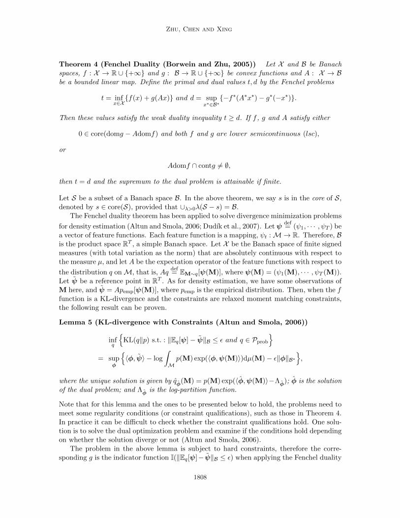
Lemma 5 (KL-divergence with Constraints (Altun and Smola, 2006))
infq
KL(q‖p) s.t. : ‖Eq[ψ]− ψ‖B ≤ ε and q ∈ Pprob
= sup
φ
〈φ, ψ〉 − log
∫Mp(M) exp(〈φ,ψ(M)〉)dµ(M)− ε‖φ‖B∗
,
where the unique solution is given by qφ(M) = p(M) exp(〈φ,ψ(M)〉−Λφ); φ is the solutionof the dual problem; and Λφ is the log-partition function.
Note that for this lemma and the ones to be presented below to hold, the problems need tomeet some regularity conditions (or constraint qualifications), such as those in Theorem 4.In practice it can be difficult to check whether the constraint qualifications hold. One solu-tion is to solve the dual optimization problem and examine if the conditions hold dependingon whether the solution diverge or not (Altun and Smola, 2006).
The problem in the above lemma is subject to hard constraints, therefore the corre-sponding g is the indicator function I(‖Eq[ψ]− ψ‖B ≤ ε) when applying the Fenchel duality
1808

Regularized Bayesian Inference and Infinite Latent SVMs
theorem. Other examples of the posterior constraints can be found in Dudık et al. (2007);Mann and McCallum (2010); Ganchev et al. (2010), as we have discussed in Section 3.2. Inthis paper, we consider the general soft constraints as defined in the RegBayes problem (5).Furthermore, we do not assume the existence of a fully observed data set to compute theempirical expectation φ. Specifically, following a similar line of reasoning as in Altun andSmola (2006), though this time with an un-normalized p in KL(q‖p), we have the followingresult. The detailed proof is deferred to Appendix C.1.
Theorem 6 (Representation theorem of RegBayes) Let E be the expectation opera-tor with feature functions ψ(M;D), and assume g is convex and lower semicontinuous (lsc).We have
infq(M)
KL(q(M)‖p(M,D)) + g(Eq) s.t. : q(M) ∈ Pprob
= sup
φ
− log
∫Mp(M,D) exp(〈φ,ψ(M;D)〉)dµ(M)− g∗(−φ)
,
where the unique solution is given by qφ(M) = p(M,D) exp(〈φ,ψ(M;D)〉 − Λφ); and φ isthe solution of the dual problem; and Λφ is the log-partition function.
From the optimum solution qφ(M), we can see that the form of the RegBayes poste-rior is symbolically similar to that of the Bayesian posterior; but instead of multiply-ing the likelihood term with a prior distribution, RegBayes introduces an extra term,exp(〈φ,ψ(M;D)〉 − Λφ), whose coefficients are derived from an constrained optimizationproblem resultant from the constraints on the posterior. We make the following remarks.
Remark 7 (Putting constraints on priors is a special case of RegBayes) If boththe feature function ψ(M;D) and φ depend on the model M only, this extra term con-tributes to define a new prior π′(M) ∝ π(M) exp(〈φ,ψ(M;D)〉 − Λφ). For example, if weconstrain the model space to a subset M0 ⊂ M a priori, this constraint can be incorpo-rated in RegBayes by defining the expectation constraint on M only. Specifically, define thesingle feature function ψ(M): ψ(M) = 0 if M ∈ M0, otherwise 1; and define the simpleposterior regularization g(Eq) = I(Eq[ψ(M)] = 0). Then, by Theorem 6,6 we have φ = −∞and qφ(M) ∝ π′(M)p(D|M), where π′(M) ∝ π(M)I(M ∈ M0) is the constrained prior.Therefore, such a constraint lets RegBayes cover the widely used truncated priors, such astruncated Gaussian (Robert, 1995).
Remark 8 (RegBayes is more flexible than Bayes’ rule) For the more general casewhere ψ(M;D) depends on both M and D, the term p(M,D) exp(〈φ,ψ(M;D)〉) implicitlydefines a joint distribution on (M,D) if it has a finite measure. In this case, RegBayesis doing implicit Bayesian conditionalization, that is, the posterior qφ(M) can be obtainedthrough Bayes’ rule with some well-defined prior and likelihood. However, it could be thatthe integral of p(M,D) exp(〈φ,ψ(M;D)〉) with respect to (M,D) is not finite because of theway φ varies with D,7 in which case there is no implicit prior and likelihood that give back
6. We also used the fact that if f(x) = I(x = c) is an indicator function, its conjugate is f∗(µ) = c · µ.7. Note: this does not affect the well-normalization of the posterior qφ(M) because its integral is taken
over M only, with D fixed.
1809

Zhu, Chen and Xing
qφ(M) through Bayesian conditionalization. Therefore, RegBayes is more flexible than thestandard Bayesian inference, where the prior and likelihood model are explicitly defined, butno additional constraints or regularization can be systematically incorporated. The recentwork (Mei et al., 2014) presents an example. Specifically, we show that incorporating domainknowledge via posterior regularization can lead to a flexible framework that automaticallylearns the importance of each piece of knowledge, thereby allowing for a robust incorporation,which is important in the scenarios where noisy knowledge is collected from crowds. Incontrast, eliciting expert knowledge via fitting some priors is generally hard, especially inhigh-dimensional spaces, as experts are normally good at perceiving low-dimensional andwell-behaved distributions but can be very bad in perceiving high-dimensional or skeweddistributions (Garthwaite et al., 2005).
It is worth mentioning that although the above theorem provides a generic representa-tion of the solution to RegBayes, in practice we usually need to make additional assumptionsin order to make either the primal or dual problem tractable to solve. Since such assump-tions could make the feasible space non-convex, additional cautions need to be paid. Forinstance, the mean-field assumptions will lead to a non-convex feasible space (Wainrightand Jordan, 2008), and we can only apply the convex analysis theory to deal with convexsub-problems within an EM-type procedure. More concrete examples will be provided lateralong the developments of various models. We should also note that the modeling flexibilityof RegBayes comes with risks. For example, it might lead to inconsistent posteriors (Barronet al., 1999; Choi and Ramamoorthi, 2008). This paper focuses on presenting several prac-tical instances of RegBayes and we leave a systematic analysis of the Bayesian asymptoticproperties (e.g., posterior consistency and convergence rates) for future work.
Now, we derive the conjugate functions of three examples which will be used shortlyfor developing the infinite latent SVM models we have intended. We defer the proof toAppendix C. Specifically, the first one is the conjugate of a simple function, which will beused in a binary latent SVM classification model.
Lemma 9 Let g0 : R→ R be defined as g0(x) = C max(0, x). Then, we have
g∗0(µ) = I(0 ≤ µ ≤ C).
The second function is slightly more complex, which will be used for defining a multi-waylatent SVM classifier. Specifically, we define the function g1 : RL → R as
g1(x) = C max(x), (8)
where max(x)def= max(x1, · · · , xL). Apparently, g1 is convex because it is a point-wise
maximum (Boyd and Vandenberghe, 2004) of the simple linear functions φi(x) = xi. Then,we have the following results.
Lemma 10 The convex conjugate of g1(x) as defined above is
g∗1(µ) = I(∀i, µi ≥ 0; and
∑i
µi = C).
1810
Regularized Bayesian Inference and Infinite Latent SVMs
Let y ∈ R and ε ∈ R+ are fixed parameters. The last function that we are interested inis g2 : R→ R, where
g2(x; y, ε) = C max(0, |x− y| − ε).
Finally, we have the following lemma, which will be used in developing large-margin regres-sion models.
Lemma 11 The convex conjugate of g2(x) as defined above is
g∗2(µ; y, ε) = µy + ε|µ|+ I(|µ| ≤ C
).
4. Infinite Latent Support Vector Machines
Given the general theoretical framework of RegBayes introduced in Section 3, now weare ready to present its application to the development of two interesting nonparametricRegBayes models. In these two models we conjoin the ideas behind the nonparametricBayesian infinite feature model known as the Indian buffet process (IBP), and the largemargin classifier known as support vector machines (SVM) to build a new class of modelsfor simultaneous single-task (or multi-task) classification and feature learning. A parametricBayesian model is presented in Appendix B.
Specifically, to illustrate how to develop latent large-margin classifiers and automaticallyresolve the unknown dimensionality of latent features from data, we demonstrate how tochoose/define the three key elements of RegBayes, that is, prior distribution, likelihoodmodel, and posterior regularization. We first present the single-task classification model.The basic setup is that we project each data example x ∈ X ⊂ RD to a latent featurevector z. Here, we consider binary features. Real-valued features can be easily consideredby elementwise multiplication of z by a Guassian vector (Griffiths and Ghahramani, 2005).Given a set of N data examples, let Z be the matrix, of which each row is a binary vector znassociated with data sample n. Instead of pre-specifying a fixed dimension of z, we resortto the nonparametric Bayesian methods and let z have an infinite number of dimensions.To make the expected number of active latent features finite, we employ an IBP as priorfor the binary feature matrix Z, as reviewed below.
4.1 Indian Buffet Process
Indian buffet process (IBP) was proposed in Griffiths and Ghahramani (2005) and hasbeen successfully applied in various fields, such as link prediction (Miller et al., 2009) andmulti-task learning (Rai and Daume III, 2010). We will make use of its stick-breakingconstruction (Teh et al., 2007), which is good for developing efficient inference methods.Let πk ∈ (0, 1) be a parameter associated with each column of the binary matrix Z. Givenπk, each znk in column k is sampled independently from Bernoulli(πk). The parameter πare generated by a stick-breaking process
π1 = ν1, and πk = νkπk−1 =k∏i=1
νi,
1811

Zhu, Chen and Xing
where νi ∼ Beta(α, 1). Since each νi is less than 1, this process generates a decreasingsequence of πk. Specifically, given a finite data set, the probability of seeing feature kdecreases exponentially with k.
IBP has several properties. For a finite number of rows, N , the prior of the IBP giveszero mass on matrices with an infinite number of ones, as the total number of columns withnon-zero entries is Poisson(αHN ), where HN is the Nth harmonic number, HN =
∑Nj=1
1j .
Thus, Z has almost surely only a finite number of non-zero entries, though this number isunbounded. A second property of IBP is that the number of features possessed by eachdata point follows a Poisson(α) distribution. Therefore, the expected number of non-zeroentries in Z is Nα.
4.2 Infinite Latent Support Vector Machines
Consider a single-task, but multi-way classification, where each training data is provided
with a categorical label y ∈ Y def= 1, · · · , L. Suppose that the latent features zn for
document n are given, then we can define the latent discriminant function as linear
f(y,xn, zn;η)def= η>g(y,xn, zn), (9)
where g(y,xn, zn) is a vector stacking L subvectors of which the yth is z>n and all the othersare zero;8 η is the corresponding infinite-dimensional vector of feature weights. Since we aredoing Bayesian inference, we need to maintain the entire distribution profile of the latentfeature matrix Z. However, in order to make a prediction on the observed data x, we needto remove the uncertainty of Z. Here, we define the effective discriminant function as anexpectation9 (i.e., a weighted average considering all possible values of Z) of the latentdiscriminant function. To fully explore the flexibility offered by Bayesian inference, we alsotreat η as random and aim to infer its posterior distribution from given data. For theprior, we assume all the dimensions of η are independent and each dimension ηk follows thestandard normal distribution. This is in fact a Gaussian process (GP) prior as η is infinitedimensional. More formally, the effective discriminant function f : X × Y 7→ R is
f(y,xn; q(Z,η,W)
) def= Eq(Z,η,W)
[f(y,xn, zn;η)
](10)
= Eq(Z,η,W)
[η>g(y,xn, zn)
],
where q(Z,η,W) is the post-data posterior distribution we want to infer. We have includedW as a place holder for any other variables we may define, e.g., the variables arising froma data likelihood model. Since we are taking the expectation, the variables which do notappear in the feature map g (i.e., W) will be marginalized out.
Before moving on, we should note that since we require q to be absolutely continuouswith respect to the prior to make the KL-divergence term well defined in the RegBayes
8. We can consider the input features xn or its certain statistics in combination with the latent features znto define a classifier boundary, by simply concatenating them in the subvectors.
9. Although other choices such as taking the mode are possible, our choice could lead to a computationallyeasy problem because expectation is a linear functional of the distribution under which the expectationis taken. Moreover, expectation can be more robust than taking the mode (Khan et al., 2010), and ithas been widely used in previous work (Zhu et al., 2009, 2011b).
1812
Regularized Bayesian Inference and Infinite Latent SVMs
problem, q(Z) will also put zero mass on Z’s with an infinite number of non-zero entries,because of the properties of the IBP prior. The sparsity of Z is essential to ensure that thedot-product in (9) and the expectation in (10) are well defined, i.e., with finite values.10
Moreover, in practice, to make the problem computationally feasible, we usually set afinite upper bound K to the number of possible features, where K is sufficiently large andknown as the truncation level (See Section 4.4 and Appendix D.2 for details). As shownin Doshi-Velez (2009), the `1-distance truncation error of marginal distributions decreasesexponentially as K increases. For a finite truncation level, all the expectations are definitelyfinite.
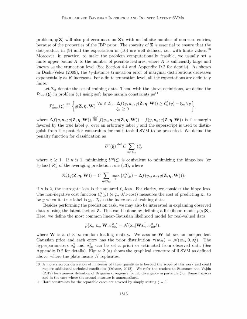
Let Itr denote the set of training data. Then, with the above definitions, we define thePpost(ξ) in problem (5) using soft large-margin constraints as11
Pcpost(ξ)def=
q(Z,η,W)
∀n ∈ Itr : ∆f(y,xn; q(Z,η,W)) ≥ `∆n (y)− ξn, ∀yξn ≥ 0
,
where ∆f(y,xn; q(Z,η,W))def= f(yn,xn; q(Z,η,W)) − f(y,xn; q(Z,η,W)) is the margin
favored by the true label yn over an arbitrary label y and the superscript is used to distin-guish from the posterior constraints for multi-task iLSVM to be presented. We define thepenalty function for classification as
U c(ξ)def= C
∑n∈Itr
ξκn,
where κ ≥ 1. If κ is 1, minimizing U c(ξ) is equivalent to minimizing the hinge-loss (or`1-loss) Rch of the averaging prediction rule (13), where
Rch(q(Z,η,W)) = C∑n∈Itr
maxy
(`∆n (y)−∆f(yn,xn; q(Z,η,W))
);
if κ is 2, the surrogate loss is the squared `2-loss. For clarity, we consider the hinge loss.The non-negative cost function `∆n (y) (e.g., 0/1-cost) measures the cost of predicting xn tobe y when its true label is yn. Itr is the index set of training data.
Besides performing the prediction task, we may also be interested in explaining observeddata x using the latent factors Z. This can be done by defining a likelihood model p(x|Z).Here, we define the most common linear-Gaussian likelihood model for real-valued data
p(xn|zn,W, σ2
n0
)= N
(xn|Wz>n , σ
2n0I),
where W is a D × ∞ random loading matrix. We assume W follows an independentGaussian prior and each entry has the prior distribution π(wdk) = N (wdk|0, σ2
0). Thehyperparameters σ2
0 and σ2n0 can be set a priori or estimated from observed data (See
Appendix D.2 for details). Figure 2 (a) shows the graphical structure of iLSVM as definedabove, where the plate means N replicates.
10. A more rigorous derivation of finiteness of these quantities is beyond the scope of this work and couldrequire additional technical conditions (Orbanz, 2012). We refer the readers to Stummer and Vajda(2012) for a generic definition of Bregman divergence (or KL divergence in particular) on Banach spacesand in the case where the second measure is unnormalized.
11. Hard constraints for the separable cases are covered by simply setting ξ = 0.
1813

Zhu, Chen and Xing
Training: Putting the above definitions together, we get the RegBayes problem foriLSVM in the following two equivalent forms
infq(Z,η,W),ξ
KL(q(Z,η,W)‖p(Z,η,W,D)) + U c(ξ) (11)
s.t. : q(Z,η,W) ∈ Pcpost(ξ)
⇐⇒ infq(Z,η,W)∈Pprob
KL(q(Z,η,W)‖p(Z,η,W,D)) +Rch(q(Z,η,W)), (12)
where p(Z,η,W,D) = π(η)π(Z)π(W)∏Nn=1 p(xn|zn,W, σ2
n0) is the joint distribution ofthe model; π(Z) is an IBP prior; and π(η) and π(W) are Gaussian process priors withidentity covariance functions.
Directly solving the iLSVM problems is not easy because either the posterior constraintsor the non-smooth regularization functionRc is hard to deal with. Thus, we resort to convexduality theory, which will be useful for developing approximate inference algorithms. Wecan either solve the constrained form (11) using Lagrangian duality theory (Ito and Kunisch,2008) or solve the unconstrained form (12) using Fenchel duality theory. Here, we take thesecond approach. In this case, the linear operator is the expectation operator, denoted byE : Pprob → R|Itr|×L and the element of Eq evaluated at y for the nth example is
Eq(n, y)def= ∆f
(y,xn; q(Z,η,W)
)= Eq(Z,η,W)
[η>∆gn(y,Z)
],
where ∆gn(y,Z)def= g(yn,xn, z)− g(y,xn, z). Then, let g1 : RL → R be a function defined
in the same form as in (8). We have
Rch(q(Z,η,W)
)=∑n∈Itr
g1
(`∆n − Eq(n)
),
where Eq(n)def= (Eq(n, 1), · · · , Eq(n,L)) and `∆n
def= (`∆n (1), · · · , `∆n (L)) are the vectors of
elements evaluated for nth data. By the Fenchel’s duality theorem and the results inLemma 10, we can derive the conjugate of the problem (12). The proof is deferred toAppendix C.4.
Lemma 12 (Conjugate of iLSVM) For the iLSVM problem, we have that
infq(Z,η,W)∈Pprob
KL(q(Z,η,W)‖p(Z,η,W,D)
)+Rch
(q(Z,η,W)
)= sup
ω− logZ(ω|D) +
∑n∈Itr
∑y
ωyn`∆n (y)−
∑n
g∗1(ωn),
where ωn = (ω1n, · · · , ωLn ) is the subvector associated with data n. Moreover, The optimum
distribution is the posterior distribution
q(Z,η,W) =1
Z(ω|D)p(Z,η,W,D) exp
∑n∈Itr
∑y
ωynη>∆gn(y, Z)
,
where Z(ω|D) is the normalization factor and ω is the solution of the dual problem.
1814

Regularized Bayesian Inference and Infinite Latent SVMs
Xn
Yn
W
Zn
N
IBP( )
(a)
Z
Xmn
Ymn
Wmn
N
M
m
m
IBP( )
(b)
Figure 2: Graphical structures of (a) infinite latent SVM (iLSVM); and (b) multi-task in-finite latent SVM (MT-iLSVM). For MT-iLSVM, the dashed nodes (i.e., ςm)illustrate the task relatedness but do not exist.
Testing: to make prediction on test examples, we put both training and test datatogether to do regularized Bayesian inference. For training data, we impose the abovelarge-margin constraints because of the awareness of their true labels, while for test data,we do the inference without the large-margin constraints since we do not know their truelabels. Therefore, the classifier q(η) is learned from the training data only, while bothtraining and testing data influence the posterior distributions of the likelihood model W.After inference, we make the prediction via the rule
y∗def= argmax
yf(y,x; q(Z,η,W)
). (13)
Note that the ability to generalize to test data relies on the fact that all the data examplesshare η and the IBP prior. We can also cast the problem as a transductive inferenceproblem by imposing additional large-margin constraints on test data (Joachims, 1999).However, the resulting problem will be generally harder to solve because it needs to resolvethe unknown labels of testing examples. We also note that the testing is different fromthe standard inductive setting (Zhu et al., 2011b), where the latent features of a new dataexample can be approximately inferred given the training data. Our empirical study showslittle difference on performance between our setting and the standard inductive setting.
4.3 Multi-Task Infinite Latent Support Vector Machines
Different from classification, which is typically formulated as a single learning task, multi-task learning aims to improve a set of related tasks through sharing statistical strengthamong these tasks, which are performed jointly. Many different approaches have beendeveloped for multi-task learning; see Jebara (2011) for a review. In particular, learning acommon latent representation shared by all the related tasks has proven to be an effectiveway to capture task relationships (Ando and Zhang, 2005; Argyriou et al., 2007; Rai andDaume III, 2010). Below, we present the multi-task infinite latent SVM (MT-iLSVM) forlearning a common binary projection matrix Z to capture the relationships among multiple
1815

Zhu, Chen and Xing
tasks. Similar as in iLSVM, we also put the IBP prior on Z to allow it to have an unboundednumber of columns.
Suppose we have M related tasks. Let Dm = (xmn, ymn)n∈Imtr be the training datafor task m. We consider binary classification tasks, where Ym = +1,−1. Extension tomulti-way classification or regression can be easily done. A naıve way to solve this learningproblem with multiple tasks is to perform the multiple tasks independently. In order to makethe multiple tasks coupled and share statistical strength, MT-iLSVM introduces a latentprojection matrix Z. If the latent matrix Z is given, we define the latent discriminantfunction for task m as
fm(xmn,Z;ηm)def= (Zηm)>xmn = η>m(Z>xmn),
where xmn is one data example in Dm and ηm is the vector of parameters for task m.The dimension of ηm is the number of columns of the latent projection matrix Z, which isunbounded in the nonparametric setting. This definition provides two views of how the Mtasks get related.
(1) If we let ςm = Zηm, then ςm is the actual parameter of task m and all ςm in differenttasks are coupled by sharing the same latent matrix Z;
(2) Another view is that each task m has its own parameters ηm, but all the tasks share thesame latent projection matrix Z to extract latent features Z>xmn, which is a projectionof the input features xmn.
As such, our method can be viewed as a nonparametric Bayesian treatment of alternatingstructure optimization (ASO) (Ando and Zhang, 2005), which learns a single projectionmatrix with a pre-specified latent dimension. Moreover, different from Jebara (2011), whichlearns a binary vector with known dimensionality to select features or kernels on x, we learnan unbounded projection matrix Z using nonparametric Bayesian techniques.
As in iLSVM, we employ a Bayesian treatment of ηm, and view it as random variables.We assume that ηm has a fully-factorized Gaussian prior, i.e., ηmk ∼ N (0, 1). Then, wedefine the effective discriminant function for task m as the expectation
fm(x; q(Z,η,W)
) def= Eq(Z,η,W)
[fm(x,Z;ηm)
]= Eq(Z,η,W)[Zηm]>x,
where W is a place holder for the variables that possibly arise from other parts of themodel. As in iLSVM, since we are taking expectation, the variables which do not appearin the feature map (i.e., W) will be marginalized out. Then, the prediction rule for task
m is naturally y∗mdef= signfm(x). Similarly, we perform regularized Bayesian inference by
defining:
UMT (ξ)def= C
∑m,n∈Imtr
ξmn
and imposing the following constraints:
PMTpost(ξ)
def=
q(Z,η,W)
∀m, ∀n ∈ Imtr : ymnEq(Z,η,W)[Zηm]>xmn ≥ 1− ξmnξmn ≥ 0
. (14)
1816

Regularized Bayesian Inference and Infinite Latent SVMs
Finally, as in iLSVM we may also be interested in explaining observed data x. Therefore,we relate Z to the observed data x by defining a likelihood model:
p(xmn|wmn,Z, λ
2mn
)= N
(xmn|Zwmn, λ
2mnI
),
where wmn is a vector. We assume that W (the collection of wmn) has an independent priorπ(W) =
∏mnN (wmn|0, σ2
m0I). Fig. 2 (b) illustrates the graphical structure of MT-iLSVM.For training, we can derive the similar convex conjugate as in the case of iLSVM. Similar
as in iLSVM, minimizing UMT (ξ) is equivalent to minimizing the hinge-loss RMTh of the
multiple binary prediction rules, where
RMTh
(q(Z,η,W)
)= C
∑m,n∈Imtr
max(
0, 1− ymnEq(Z,η,W)[Zηm]>xmn
).
Thus, the RegBayes problem of MT-iLSVM can be equivalently written as
infq(Z,η,W)
KL(q(Z,η,W)‖p(Z,η,W,D)
)+RMT
h
(q(Z,η,W)
). (15)
Then, by the Fenchel’s duality theorem and Lemma 9, we can derive the conjugate ofMT-iLSVM. The proof is deferred to Appendix C.5.
Lemma 13 (Conjugate of MT-iLSVM) For the MT-iLSVM problem, we have that
infq(Z,η,W)∈Pprob
KL(q(Z,η,W)‖p(Z,η,W,D)) +RMTh (q(Z,η,W))
= supω
− logZ ′(ω|D) +∑m,n
ωmn −∑m,n
g∗0(ωmn).
Moreover, The optimum distribution is the posterior distribution
q(Z,η,W) =1
Z ′(ω|D)p(Z,η,W,D) exp
∑m,n
ymnωmn(Zηm)>xmn
,
where Z ′(ω|D) is the normalization factor and ω is the solution of the dual problem.
For testing, we use the same strategy as in iLSVM to do Bayesian inference on bothtraining and test data. The difference is that training data are subject to large-marginconstraints, while test data are not. Similarly, the hyper-parameters σ2
m0 and λ2mn can be
set a priori or estimated from data (See Appendix D.1 for details).
4.4 Inference with Truncated Mean-Field Constraints
Now we discuss how to perform regularized Bayesian inference with the large-margin con-straints for both iLSVM and MT-iLSVM. From the primal-dual formulations, it is obviousthat there are basically two methods to perform the regularized Bayesian inference. Oneis to directly solve the primal problem for the posterior distribution q(Z,η,W), and theother is to first solve the dual problem for the optimum ω and then infer the posteriordistribution. However, both the primal and dual problems are intractable for iLSVM and
1817

Zhu, Chen and Xing
Algorithm 1 Inference Algorithm for Infinite Latent SVMs
1: Input: corpus D and constants (α,C).2: Output: posterior distribution q(ν,Z,η,W).3: repeat4: infer q(ν), q(W) and q(Z) with q(η) and ω given;5: infer q(η) and solve for ω with q(Z) given.6: until convergence
MT-iLSVM. The intrinsic hardness is due to the mutual dependency among the latent vari-ables in the desired posterior distribution. Therefore, a natural approximation method isthe mean field (Jordan et al., 1999), which breaks the mutual dependency by assuming thatq is of some factorization form. This method approximates the original problems by impos-ing additional constraints. An alternative method is to apply approximate methods (e.g.,MCMC sampling) to infer the true posterior distributions derived via convex conjugatesas above, and iteratively estimate the dual parameters using approximate statistics (e.g.,feature expectations estimated using samples) (Schofield, 2006). Below, we use MT-iLSVMas an example to illustrate the idea of the first strategy. A full discussion on the secondstrategy is beyond the scope of this paper. For iLSVM, the similar procedure applies andwe defer its details to Appendix D.2.
To make the problem easier to solve, we use the stick-breaking representation of IBP,which includes the auxiliary variable ν, and infer the augmented posterior q(ν,W,Z,η).The joint model distribution is now q(ν,W,Z,η,D). Furthermore, we impose the truncatedmean-field constraint that
q(ν,W,Z,η) = q(η)
K∏k=1
(q(νk|γk)
D∏d=1
q(zdk|ψdk))∏mn
q(wmn|Φmn, σ
2mnI
), (16)
where K is the truncation level, and we assume that
q(νk|γk) = Beta(γk1, γk2),
q(zdk|ψdk) = Bernoulli(ψdk),
q(wmn|Φmn, σ2mnI) = N (wmn|Φmn, σ
2mnI).
Then, we can use the duality theory12 to solve the RegBayes problem by alternating betweentwo substeps, as outlined in Algorithm 1 and detailed below.
Infer q(ν), q(W) and q(Z): Since q(ν) and q(W) are not directly involved in theposterior constraints, we can solve for them by using standard Bayesian inference, i.e.,minimizing a KL-divergence. Specifically, for q(W), since the prior is also normal, we caneasily derive the update rules for Φmn and σ2
mn. For q(ν), we have the same update rulesas in Doshi-Velez (2009). We defer the details to Appendix D.1.
12. Lagrangian duality (Ito and Kunisch, 2008) was used in Zhu et al. (2011a) to solve the constrainedvariational formulations, which is closely related to Fenchel duality (Magnanti, 1974) and leads to thesame solutions for iLSVM and MT-iLSVM.
1818

Regularized Bayesian Inference and Infinite Latent SVMs
For q(Z), it is directly involved in the posterior constraints. So, we need to solve ittogether with q(η) using conjugate theory. However, this is intractable. Here, we adopt analternating strategy that first infers q(Z) with q(η) and dual parameters ω fixed, and theninfers q(η) and solves for ω. Specifically, since the large-margin constraints are linear ofq(Z), we can get the mean-field update equation as
ψdk =1
1 + e−ϑdk,
where
ϑdk =
k∑j=1
Eq[log vj ]− Lνk −∑mn
1
2λ2mn
((Kσ2
mn + (φkmn)2)
−2xdmnφkmn + 2
∑j 6=k
φjmnφkmnψdj
)+
∑m,n∈Imtr
ymnEq[ηmk]xdmn,
and Lνk is an lower bound of Eq[log(1−∏kj=1 vj)] (See Appendix D.1 for details). The last
term of ϑdk is due to the large-margin posterior constraints as defined in (14). Therefore,from this equation we can see how the large-margin constraints regularize the procedure ofinferring the latent matrix Z.
Infer q(η) and solve for ω: Now, we can apply the convex conjugate theory and showthat the optimum posterior distribution of η is
q(η) =∏m
q(ηm), where q(ηm) ∝ π(ηm) expη>mµm
,
and µm =∑
n∈Imtrymnωmn(ψ>xmn). Here, we assume π(ηm) is standard normal. Then, we
have q(ηm) = N (ηm|µm, I) and the optimum dual parameters can be obtained by solvingthe following M independent dual problems
supωm
−1
2µ>mµm +
∑n∈Imtr
ωmn
∀n ∈ Imtr , s.t. : 0 ≤ ωmn ≤ C,
where the constraints are from the conjugate function g∗0 in Lemma 13. These dual problems(or their primal forms) can be efficiently solved with a binary SVM solver, such as SVM-lightor LibSVM.
5. Experiments
We present empirical results for both classification and multi-task learning. Our resultsappear to demonstrate the merits inherited from both Bayesian nonparametrics and large-margin learning.
5.1 Multi-way Classification
We evaluate the infinite latent SVM (iLSVM) for classification on the real TRECVID2003and Flickr image data sets, which have been extensively evaluated in the context of learning
1819

Zhu, Chen and Xing
TRECVID2003 FlickrModel Accuracy F1 score Accuracy F1 score
EFH+SVM 0.565 ± 0.0 0.427 ± 0.0 0.476 ± 0.0 0.461 ± 0.0MMH 0.566 ± 0.0 0.430 ± 0.0 0.538 ± 0.0 0.512 ± 0.0
IBP+SVM 0.553 ± 0.013 0.397 ± 0.030 0.500 ± 0.004 0.477 ± 0.009iLSVM 0.563 ± 0.010 0.448 ± 0.011 0.533 ± 0.005 0.510 ± 0.010
Table 1: Classification accuracy and F1 scores on the TRECVID2003 and Flickr imagedata sets (Note: MMH and EFH have zero std because of their deterministicinitialization).
10 20 30 40 50 60 70 80
0.2
0.3
0.4
0.5
0.6
K
Accu
racy
10 20 30 40 50 60 70 80
0.2
0.3
0.4
0.5
0.6
K
F1
sco
re
Figure 3: Accuracy and F1 score of MMH on the Flickr data set with different numbers oflatent features.
finite latent feature models (Chen et al., 2012). TRECVID2003 consists of 1078 video key-frames that belong to 5 categories, including Airplane scene, Basketball scene, Weathernews, Baseball scene, and Hockey scene. Each data example has two types of features,including a 1894-dimension binary vector of text features and a 165-dimension HSV colorhistogram. The Flickr image data set consists of 3411 natural scene images about 13 typesof animals, including squirrel, cow, cat, zebra, tiger, lion, elephant, whales, rabbit, snake,antlers, hawk and wolf, downloaded from the Flickr website.13 Also, each example has twotypes of features, including 500-dimension SIFT bag-of-words and 634-dimension real-valuedfeatures (e.g., color histogram, edge direction histogram, and block-wise color moments).Here, we consider the real-valued features only by defining Gaussian likelihood distributionsfor x; and we define the discriminant function using latent features only as in (9). We followthe same training/testing splits as in Chen et al. (2012).
We compare iLSVM with the large-margin Harmonium (MMH) (Chen et al., 2012),which was shown to outperform many other latent feature models, and two decoupledapproaches of EFH+SVM and IBP+SVM. EFH+SVM uses the exponential family Harmo-
13. The website is available at: http://www.flickr.com/.
1820

Regularized Bayesian Inference and Infinite Latent SVMs
0 10 20 30 40 50 600
0.2
0.4
0.6
0.8
1
Ove
rall
Avg
Valu
e
0 10 20 30 40 50 600
0.2
0.4
0.6
0.8
1
Per−
class
Avg
Valu
e
Feature ID
class−1
class−2
class−3
class−4
class−5
Figure 4: (Up) the overall average values of the latent features with standard deviationover different classes; and (Bottom) the per-class average values of latent featureslearned by iLSVM on the TRECVID data set.
0 20 40 60 80 100 120 140 160 180 2000
0.2
0.4
0.6
0.8
1
Ove
rall
Avg
Valu
e
Feature ID
Figure 5: The overall average values of the latent features with standard deviation overdifferent classes on the Flickr data set.
nium (EFH) (Welling et al., 2004) to discover latent features and then learns a multi-waySVM classifier. IBP+SVM is similar, but uses an IBP factor analysis model to discoverlatent features (Griffiths and Ghahramani, 2005). To initialize the learning algorithms forthese models, we found that using the SVD factors of the input feature matrix as the ini-tial weights for MMH and EFH can produce better results. Here, we also use the SVDfactors as the initial mean of weights in the likelihood models for iLSVM. Both MMH andEFH+SVM are finite models and they need to pre-specify the dimensionality of latent fea-tures. We report their results on classification accuracy and F1 score (i.e., the averageF1 score over all possible classes) (Zhu et al., 2011b) achieved with the best dimensional-ity in Table 1. Figure 3 illustrates the performance change of MMH when using differentnumber of latent features, from which we can see that K = 40 produces the best per-formance and either increasing or decreasing K could make the performance worse. For
1821

Zhu, Chen and Xing
F1
F2
F3
F4
F5
F6
Figure 6: Six example features discovered iLSVM on the Flickr animal data set. For eachfeature, we show 5 top-ranked images.
iLSVM and IBP+SVM, we use the mean-field inference method and present the averageperformance with 5 randomly initialized runs (Please see Appendix D.2 for the algorithmand initialization details). We perform 5-fold cross-validation on training data to selecthyperparameters, e.g., α and C (we use the same procedure for MT-iLSVM). We can seethat iLSVM can achieve comparable performance with the nearly optimal MMH, withoutneeding to pre-specify the latent feature dimension,14 and is much better than the decoupledapproaches (i.e., IBP+SVM and EFH+SVM). For the two stage methods, we don’t havea clear winner—IBP+SVM performs a bit worse than EFH+SVM on the TRECVID dataset, while it outperforms EFH+SVM on the flickr data set. The reason for the differencemay be due to the initialization or different properties of the data.
It is also interesting to examine the discovered latent features. Figure 4 shows the overallaverage values of latent features and the per-class average feature values of iLSVM in onerun on the TRECVID data set. We can see that on average only about 45 features areactive for the TRECVID data set. For the overall average, we also present the standarddeviation over the 5 categories. A larger deviation means that the corresponding featureis more discriminative when predicting different categories. For example, feature 26 andfeature 34 are generally less discriminative than many other features, such as feature 1
14. We set the truncation level to 300, which is sufficiently large.
1822

Regularized Bayesian Inference and Infinite Latent SVMs
and feature 30. Figure 5 shows the overall average feature values together with standarddeviation on the Flickr data set. We omitted the per-class average because that figure istoo crowded with 13 categories. We can that as k increases, the probability that feature kis active decreases. The reason for the features with stable values (i.e., standard deviationsare extremely small) is due to our initialization strategy (each feature has 0.5 probabilityto be active). Initializing ψdk as being exponentially decreasing (e.g., like the constructingprocess of π) leads to a faster decay and many features will be inactive. To examine thesemantics of each feature,15 Figure 6 presents some example features discovered on theFlickr animal data set. For each feature, we present 5 top-ranked images which have largevalues on this particular feature. We can see that most of the features are semanticallyinterpretable. For instance, feature F1 is about squirrel; feature F2 is about ocean animal,which is whales in the Flickr data set; and feature F4 is about hawk. We can also see thatsome features are about different aspects of the same category. For example, feature F2and feature F3 are both about whales, but with different background.
5.2 Multi-task Learning
Now, we evaluate the multi-task infinite latent SVM (MT-iLSVM) on several well-studiedreal data sets.
5.2.1 Description of the Data
Scene and Yeast Data: These data sets are from the UCI repository, and each dataexample has multiple labels. As in Rai and Daume III (2010), we treat the multi-labelclassification as a multi-task learning problem, where each label assignment is treated asa binary classification task. The Yeast data set consists of 1500 training and 917 testexamples, each having 103 features, and the number of labels (or tasks) per example is 14.The Scene data set consists 1211 training and 1196 test examples, each having 294 features,and the number of labels (or tasks) per example for this data set is 6.
School Data: This data set comes from the Inner London Education Authority andhas been used to study the effectiveness of schools. It consists of examination recordsof 15,362 students from 139 secondary schools in years 1985, 1986 and 1987. The dataset is publicly available and has been extensively evaluated in various multi-task learningmethods (Bakker and Heskes, 2003; Bonilla et al., 2008; Zhang and Yeung, 2010), whereeach task is defined as predicting the exam scores of students belonging to a specific schoolbased on four student-dependent features (year of the exam, gender, VR band and ethnicgroup) and four school-dependent features (percentage of students eligible for free schoolmeals, percentage of students in VR band 1, school gender and school denomination). Inorder to compare with the above methods, we follow the same setup described by Argyriouet al. (2007) and Bakker and Heskes (2003) and similarly we create dummy variables forthose features that are categorical forming a total of 19 student-dependent features and 8school-dependent features. We use the same 10 random splits16 of the data, so that 75%of the examples from each school (task) belong to the training set and 25% to the test set.
15. The interpretation of latent features depends heavily on the input data.16. The splits are available at: http://ttic.uchicago.edu/~argyriou/code/index.html.
1823

Zhu, Chen and Xing
Data set Model Acc F1-Micro F1-Macro
Yeast
YaXue 0.5106 0.3897 0.4022Piyushrai-1 0.5212 0.3631 0.3901Piyushrai-2 0.5424 0.3946 0.4112
MT-IBP+SVM 0.5475 ± 0.005 0.3910 ± 0.006 0.4345 ± 0.007MT-iLSVM 0.5792 ± 0.003 0.4258 ± 0.005 0.4742 ± 0.008
Scene
YaXue 0.7765 0.2669 0.2816Piyushrai-1 0.7756 0.3153 0.3242Piyushrai-2 0.7911 0.3214 0.3226
MT-IBP+SVM 0.8590 ± 0.002 0.4880 ± 0.012 0.5147 ± 0.018MT-iLSVM 0.8752 ± 0.004 0.5834 ± 0.026 0.6148 ± 0.020
Table 2: Multi-label classification performance on Scene and Yeast data sets.
On average, the training set includes about 80 students per school and the test set about30 students per school.
5.2.2 Results
Scene and Yeast Data: We compare with the closely related nonparametric Bayesianmethods, including kernel stick-breaking (YaXue) (Xue et al., 2007) and the basic andaugmented infinite predictor subspace models (i.e., Piyushrai-1 and Piyushrai-2) proposedby Rai and Daume III (2010). These nonparametric Bayesian models were shown to out-perform the independent Bayesian logistic regression and a single-task pooling approachin previous work (Rai and Daume III, 2010). We also compare with a decoupled methodMT-IBP+SVM that uses an IBP factor analysis model to find shared latent features amongmultiple tasks and then builds separate SVM classifiers for different tasks.17 For MT-iLSVM and MT-IBP+SVM, we use the mean-field inference method in Sec 4.4 and reportthe average performance with 5 randomly initialized runs (See Appendix D.1 for initializa-tion details). For comparison with Rai and Daume III (2010) and Xue et al. (2007), weuse the overall classification accuracy, F1-Macro and F1-Micro as performance measures.Table 2 shows the results. On both data sets, MT-iLSVM needs less than 50 latent fea-tures on average. We can see that the large-margin MT-iLSVM performs much better thanother nonparametric Bayesian methods and MT-IBP+SVM, which separates the inferenceof latent features from learning the classifiers.
School Data: We use the percentage of explained variance (Bakker and Heskes, 2003)as the measure of the regression performance, which is defined as the total variance of thedata minus the sum-squared error on the test set as a percentage of the total variance.Since we use the same settings, we can compare with the state-of-the-art results of
(1) Bayesian multi-task learning (BMTL) (Bakker and Heskes, 2003);
(2) Multi-task Gaussian processes (MTGP) (Bonilla et al., 2008);
17. This decoupled approach is in fact an one-iteration MT-iLSVM, where we first infer the shared latentmatrix Z and then learn an SVM classifier for each task.
1824

Regularized Bayesian Inference and Infinite Latent SVMs
15
20
25
30
35
Exp
lain
ed
Va
ria
nce
(%
)
STL
BMTL
MTGP
MTRL
MT−IBP+SVM
MT−IBP+SVMf
MT−iLSVM
MT−iLSVMf
Figure 7: Percentage of explained variance by various models on the School data set.
(3) Convex multi-task relationship learning (MTRL) (Zhang and Yeung, 2010);
and single-task learning (STL) as reported in Bonilla et al. (2008) and Zhang and Yeung(2010). For MT-iLSVM and MT-IBP+SVM, we also report the results achieved by usingboth the latent features (i.e., Z>x) and the original input features x through vector concate-nation, and we denote the corresponding methods by MT-iLSVMf and MT-IBP+SVMf ,respectively. On average the multi-task latent SVM (i.e., MT-iLSVM) needs about 50 latentfeatures to get sufficiently good and robust performance. From the results in Figure 7, wecan see that the MT-iLSVM achieves better results than the existing methods that havebeen tested in previous studies. Again, the joint MT-iLSVM performs much better thanthe decoupled method MT-IBP+SVM, which separates the latent feature inference from thetraining of large-margin classifiers. Finally, using both latent features and the original inputfeatures can boost the performance slightly for MT-iLSVM, while much more significantlyfor the decoupled MT-IBP+SVM.
5.3 Sensitivity Analysis
Figure 8 shows how the performance of MT-iLSVM changes against the hyper-parameterα and regularization constant C on the Yeast and School data sets. We can see that onthe Yeast data set, MT-iLSVM is insensitive to both α and C. For the School data set,MT-iLSVM is very insensitive the α, and it is stable when C is set between 0.3 and 1.
Figure 9 shows how the training size affects the performance and running time of MT-iLSVM on the School data set. We use the first b% (b = 50, 60, 70, 80, 90, 100) of the trainingdata in each of the 10 random splits as training set and use the corresponding test dataas test set. We can see that as training size increases, the performance and running timegenerally increase; and MT-iLSVM achieves the state-of-art performance when using about70% training data. From the running time, we can also see that MT-iLSVM is generallyquite efficient by using mean-field inference.
Finally, we investigate how the performance of MT-iLSVM changes against the hyper-parameters σ2
m0 and λ2mn. We initially set σ2
m0 = 1 and compute λ2mn from observed data.
If we further estimate them by maximizing the objective function, the performance does
1825
Zhu, Chen and Xing
1 2 3 4 5 6
0.565
0.57
0.575
0.58
0.585
0.59
sqrt of α
Acc
ura
cy
(a) Yeast
0 1 2 3 4 5 6
0.565
0.57
0.575
0.58
0.585
0.59
sqrt of C
Acc
ura
cy
(b) Yeast
1 2 3 4 5 625
26
27
28
29
30
31
32
33
34
35
sqrt of α
Exp
lain
ed v
ariance
(%
)
(c) School
0 0.5 1 1.5 2 2.515
20
25
30
35
C
Exp
lain
ed
va
ria
nce
(%
)
(d) School
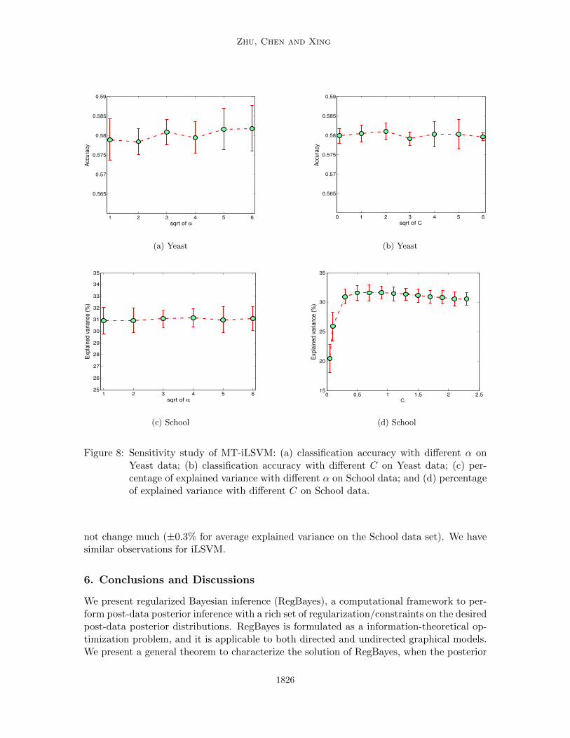
Figure 8: Sensitivity study of MT-iLSVM: (a) classification accuracy with different α onYeast data; (b) classification accuracy with different C on Yeast data; (c) per-centage of explained variance with different α on School data; and (d) percentageof explained variance with different C on School data.
not change much (±0.3% for average explained variance on the School data set). We havesimilar observations for iLSVM.
6. Conclusions and Discussions
We present regularized Bayesian inference (RegBayes), a computational framework to per-form post-data posterior inference with a rich set of regularization/constraints on the desiredpost-data posterior distributions. RegBayes is formulated as a information-theoretical op-timization problem, and it is applicable to both directed and undirected graphical models.We present a general theorem to characterize the solution of RegBayes, when the posterior
1826

Regularized Bayesian Inference and Infinite Latent SVMs
40 50 60 70 80 90 100 11022
23
24
25
26
27
28
29
30
31
32
33
Percentage of Training Data
Exp
lain
ed V
ariance
(%
)
40 50 60 70 80 90 100 110200
300
400
500
600
700
800
900
1000
1100
Percentage of Training Data
Runnin
g T
ime (
sec)
Figure 9: Percentage of explained variance and running time by MT-iLSVM with varioustraining sizes.
regularization is induced from a linear operator (e.g., expectation). Furthermore, we par-ticularly concentrate on developing two large-margin nonparametric Bayesian models underthe RegBayes framework to learn predictive latent features for classification and multi-tasklearning, by exploring the large-margin principle to define posterior constraints. Both mod-els allow the latent dimension to be automatically resolved from the data. The empiricalresults on several real data sets appear to demonstrate that our methods inherit the meritsfrom both Bayesian nonparametrics and large-margin learning.
RegBayes offers a flexible framework for considering posterior regularization in perform-ing parametric or nonparametric Bayesian inference. For future work, we plan to study otherposterior regularization beyond the large-margin constraints, such as posterior constraintsdefined on manifold structures (Huh and Fienberg, 2012) and those represented in the formof first-order logic, and investigate how posterior regularization can be used in other inter-esting nonparametric Bayesian models (Beal et al., 2002; Teh et al., 2006; Blei and Frazier,2010) in different contexts, such as link prediction (Miller et al., 2009) for social networkanalysis and low-rank matrix factorization for collaborative prediction. Some of our pre-liminary results (Xu et al., 2012; Zhu, 2012; Mei et al., 2014) have shown great promise.It is interesting to investigate more carefully along this direction. Moreover, as we havestated, RegBayes can be developed for undirected MRFs. But the inference would be evenharder. We plan to do a systematic investigation along this direction too. We have somepreliminary results presented in Chen et al. (2014), but there is a lot of room to furtherimprove. Finally, regularized Bayesian inference in general leads to a highly nontrivial infer-ence problem. Although the general solution can be derived with convex analysis theory, itis normally intractable to infer them directly. Therefore, approximate inference techniquessuch as the truncated mean-field approximation have to be used. For the current truncatedinference methods, one key limit is to pre-specify the truncation level. A too conservativetruncation level could lead to a waste of computing resources. So, it is important to develop
1827

Zhu, Chen and Xing
inference algorithms that could adaptively determine the number of latent features, such asMonte Carlo methods. We have some preliminary progress along this direction as reportedin Jiang et al. (2012) and Zhu et al. (2013). It is interesting to extend these techniques todeal with other challenging nonparametric Bayesian models.
Acknowledgements
We thank the anonymous reviewers and editors for many helpful comments to improvethe manuscript. NC and JZ are supported by National Key Foundation R&D Projects(No.s 2013CB329403, 2012CB316301), National Natural Science Foundation of China (Nos.61322308, 61332007, 61305066), Tsinghua University Initiative Scientific Research Program(No. 20121088071), a Microsoft Research Asia Research Fund (No. 20123000007), and theChina Postdoctoral Science Foundation Grant (No. 2013T60117) to NC. EX is supportedby AFOSR FA95501010247, ONR N000140910758, NSF Career DBI-0546594 and an AlfredP. Sloan Research Fellowship.
Appendix A. Generalization Beyond Bayesian Networks
Standard Bayesian inference and the proposed regularized Bayesian inference implicitlymake the assumption that the model can be graphically drawn as a Bayesian network asillustrated in Figure 10(a).18 Here, we consider a more general formulation which couldcover both directed and undirected latent variable models, such as the well-studied Boltz-mann machines (Murray and Ghahramani, 2004; Welling et al., 2004), as well as the casewhere a model could have some unknown parameters (e.g., hyper-parameters) and needan estimation procedure, such as maximum likelihood estimation (MLE), besides posteriorinference. The latter is also known as empirical Bayesian methods, which are frequentlyemployed by practitioners.
Extension 1: Empirical Bayesian Inference with Unknown Parameters: Asillustrated in Figure 10(b), in some cases we need to perform the empirical Bayesian infer-ence in the presence of unknown parameters. For instance, in a linear-Gaussian Bayesianmodel, we may choose to estimate its covariance matrix using MLE; and in a latent Dirichletallocation (LDA) (Blei et al., 2003) model, we may choose to estimate the unknown topicaldictionary, although in principle we can treat these parameters as random variables andperform full Bayesian inference. In such cases, we need some mechanisms to estimate theunknown parameters when doing Bayesian inference. Let Θ be model parameters. We canformulate empirical Bayesian inference as solving19
infΘ,q(M)
KL(q(M)‖π(M))−∫M
log p(D|M,Θ)q(M)dM (17)
s.t. : q(M) ∈ Pprob.
18. The structure within M can be arbitrary, either a directed, undirected or hybrid chain graph.19. The objective can be derived using variational techniques. It is in fact a variational upper bound of the
negative log-likelihood.
1828

Regularized Bayesian Inference and Infinite Latent SVMs
M
D
(a)
D
M
(b)
D
M
Z H
(c)
Figure 10: Illustration graphs for three different types of models that involve Bayesianinference: (a) a Bayesian generative model; (b) a Bayesian generative modelwith unknown parameters Θ; and (c) a chain graph model.
Although the problem is convex over q(M) for any fixed Θ, it is not jointly convex in general.A natural algorithm to solve this problem is the well-known EM procedure (Dempster et al.,1977), which converges to a local optimum. Specifically, we have the following result.
Lemma 14 For problem (17), the optimum solution of q(M) is equivalent to the posteriordistribution by Bayes’ theorem for any Θ; and the optimum Θ∗ is the MLE
Θ∗ = argmaxΘ
log p(D|Θ).
Proof According to the variational formulation of Bayes’ rule in (4), we get that the op-timum solution is q(M) = p(M|D,Θ) for any Θ. Substituting the optimum solution of qinto the objective, we get the optimization problem of Θ.
Extension 2: Chain Graph: In the above cases, we have assumed that the observeddata are generated by some model in a directed causal sense. This assumption holds indirected latent variable models. However, in many cases, we may choose alternative for-mulations to define the joint distribution of a model and the observed data. Figure 10(c)illustrates one such scenario, where the model M consists of two subsets of random vari-ables. One subset H is connected to the observed data via an undirected graph and theother subset Z is connected to the observed data and H using directed edges. This graph isknown as a chain graph. Due to the Markov properties of chain graph (Frydenberg, 1990),we know that the joint distribution has the factorization form as
p(M,D) = p(Z)p(H,D|Z), (18)
where p(H,D|Z) is a Markov random field (MRF). One concrete example of such a hybridchain model is the Bayesian Boltzman machines (Murray and Ghahramani, 2004), which
1829

Zhu, Chen and Xing
treat the parameters of a Boltzmann machine as random variables and perform Bayesianinference with MCMC sampling methods.
The insights that RegBayes covers undirected or chain graph latent variable models comefrom the observation that the objective L(q(M)) of problem (4) is in fact an KL-divergence,namely, we can show that
L(q(M)) = KL(q(M)‖p(M,D)), (19)
where p(M,D) is the joint distribution. Note that when D is given, the distribution p(M,D)is non-normalized for M; and we have abused the KL notation for non-normalized distri-butions in (19), but with the same formula. For directed Bayesian networks (Zhu et al.,2011a), we naturally have p(M,D) = π(M)p(D|M). For the undirected MRF models, wehave M = Z,H and again we can define the joint distribution as in (18).
Putting the above two extensions of Bayesian inference together, the regularized Bayesianinference with estimating unknown model parameters can be generally formulated as
infΘ,q(M),ξ
L(Θ, q(M)) + U(ξ) or infΘ,q(M)
L(Θ, q(M)) + g(Eq(M)) (20)
s.t. : q(M) ∈ Ppost(ξ) s.t. : q(M) ∈ Pprob,
where L(Θ, q(M)) is the objective function of problem (17). These two formulations areequivalent. We will call the former a constrained formulation and call the latter an uncon-strained formulation by ignoring the standard normalization constraints, which are easy todeal with.
Appendix B. MedLDA—A RegBayes Model with Finite Latent Features
This section presents a new interpretation of MedLDA (maximum entropy discriminationlatent Dirichlet allocation) (Zhu et al., 2009) under the framework of regularized Bayesianinference. MedLDA is a max-margin supervised topic model, an extension of latent Dirichletallocation (LDA) (Blei et al., 2003) for supervised learning tasks. In MedLDA, each dataexample is projected to a point in a finite dimensional latent space, of which each featurecorresponds to a topic, i.e., a unigram distribution over the terms in a vocabulary. MedLDArepresents each data as a probability distribution over the features, which results in aconservation constraint (i.e., the more a data expresses on one feature, the less it can expressothers) (Griffiths and Ghahramani, 2005). The infinite latent feature models discussed inSection 4 do not have such a constraint.
Without loss of generality, we consider the MedLDA regression model as an example(classification model is similar), whose graphical structure is shown in Figure 11. We assumethat all data examples have the same length V for notation simplicity. Each document is as-sociated with a response variable Y , which is observed in the training phase but unobservedin testing. We will use y to denote an instance value of Y . Let K be the number of topicsor the dimensionality of the latent topic space. MedLDA builds an LDA model to describethe observed words. The generating process of LDA is that each document n has a mixingproportion θn ∼ Dirichlet(α); each word wnm is associated with a topic znm ∼ θn, whichindexes the topic that generates the word, i.e., wnm ∼ βznm
. Define Zn = 1V
∑Vm=1 Znm
as the average topic assignment for document n. Let Θ = α,β, δ2 denote the unknown
1830
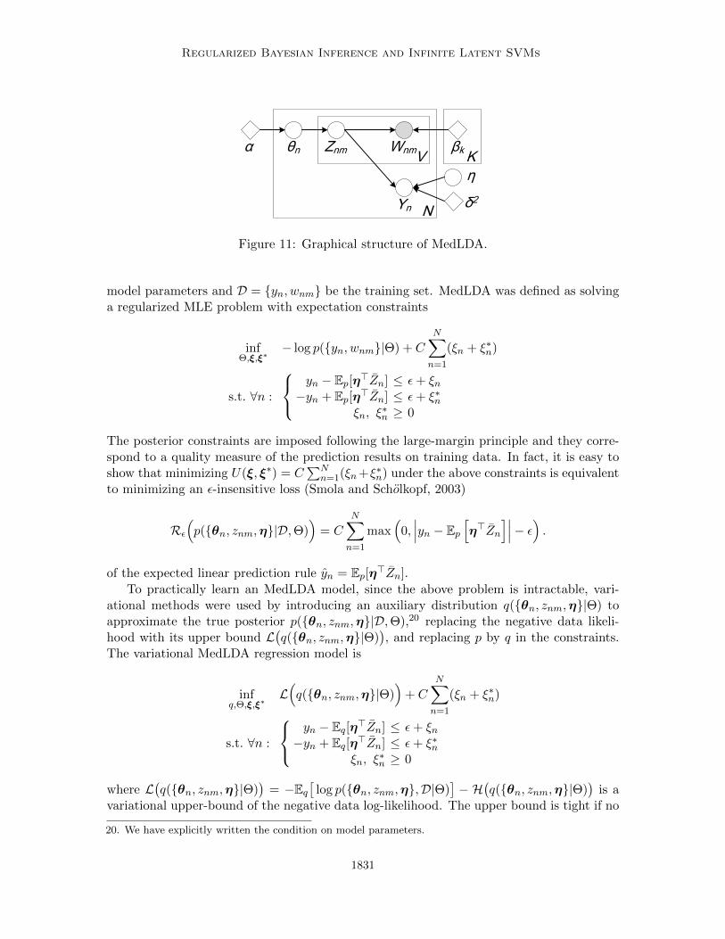
Regularized Bayesian Inference and Infinite Latent SVMs
N
VWnmZnmn
Yn
kK
2
Figure 11: Graphical structure of MedLDA.
model parameters and D = yn, wnm be the training set. MedLDA was defined as solvinga regularized MLE problem with expectation constraints
infΘ,ξ,ξ∗
− log p(yn, wnm|Θ) + CN∑n=1
(ξn + ξ∗n)
s.t. ∀n :
yn − Ep[η>Zn] ≤ ε+ ξn−yn + Ep[η>Zn] ≤ ε+ ξ∗n
ξn, ξ∗n ≥ 0
The posterior constraints are imposed following the large-margin principle and they corre-spond to a quality measure of the prediction results on training data. In fact, it is easy toshow that minimizing U(ξ, ξ∗) = C
∑Nn=1(ξn+ξ∗n) under the above constraints is equivalent
to minimizing an ε-insensitive loss (Smola and Scholkopf, 2003)
Rε(p(θn, znm,η|D,Θ)
)= C
N∑n=1
max(
0,∣∣∣yn − Ep
[η>Zn
]∣∣∣− ε) .of the expected linear prediction rule yn = Ep[η>Zn].
To practically learn an MedLDA model, since the above problem is intractable, vari-ational methods were used by introducing an auxiliary distribution q(θn, znm,η|Θ) toapproximate the true posterior p(θn, znm,η|D,Θ),20 replacing the negative data likeli-hood with its upper bound L
(q(θn, znm,η|Θ)
), and replacing p by q in the constraints.
The variational MedLDA regression model is
infq,Θ,ξ,ξ∗
L(q(θn, znm,η|Θ)
)+ C
N∑n=1
(ξn + ξ∗n)
s.t. ∀n :
yn − Eq[η>Zn] ≤ ε+ ξn−yn + Eq[η>Zn] ≤ ε+ ξ∗n
ξn, ξ∗n ≥ 0
where L(q(θn, znm,η|Θ)
)= −Eq
[log p(θn, znm,η,D|Θ)
]− H
(q(θn, znm,η|Θ)
)is a
variational upper-bound of the negative data log-likelihood. The upper bound is tight if no
20. We have explicitly written the condition on model parameters.
1831

Zhu, Chen and Xing
restricting constraints are made on the variational distribution q. In practice, additionalassumptions (e.g., mean-field) can be made on q to derive a practical approximate algorithm.
Based on the previous discussions on the extensions of RegBayes and the duality inLemma 14, we can reformulate the MedLDA regression model as an example of RegBayes.Specifically, for the MedLDA regression model, we have M = θn, znm,η. Accordingto (19), we can easily show that
L(q(θn, znm,η|Θ)
)= KL
(q(θn, znm,η|Θ)‖p(θn, znm,η, wnm, yn|Θ)
)= LB
(Θ, q(M|Θ)
).
Then, the MedLDA problem is a RegBayes model in (20) with
PMedLDApost (Θ, ξ, ξ∗)
def=
q(θn, znm,η|Θ)∀n : yn − Eq[η>Zn]≤ ε+ ξn−yn + Eq[η>Zn]≤ ε+ ξ∗n
ξn, ξ∗n≥ 0
. (21)
For the MedLDA problem, we can use Lagrangian methods to solve the constrained for-mulation. Alternatively, we can use the convex duality theorem to solve an equivalent uncon-strained form. For the variational MedLDA, the ε-insensitive loss is Rε(q(θn, znm,η|Θ)).Its conjugate can be derived using the results of Lemma 11. Specifically, we have thefollowing result, whose proof is deferred to Appendix C.6.
Lemma 15 (Conjugate of MedLDA) For the variational MedLDA problem, we have
infΘ,q(θn,znm,η|Θ)∈Pprob
L (q(θn, znm,η|Θ),Θ) +Rε (q(θn, znm,η|Θ))
= supω
− logZ ′(ω,Θ∗)−∑n
g∗2(ωn;−yn + ε, yn + ε),
where ωn = (ωn, ω′n). Moreover, The optimum distribution is the posterior distribution
q(θn, znm,η|Θ∗) =1
Z ′(ω,Θ∗|D)p (θn, znm,η,D|Θ∗) exp
∑n
(ωn − ω′n)η>zn
,(22)
where Z ′(ω,Θ|D) is the normalization factor and the optimum parameters are
Θ∗ = argmaxΘ
log p(D|Θ).
Note that although in general, either the primal or the dual problem is hard to solveexactly, the above conjugate results are still useful when developing approximate inferencealgorithms. For instance, we can impose additional mean-field assumptions on q in the pri-mal formulation and iteratively solve for each factor; and in this process convex conjugatesare useful to deal with the large-margin constraints (Zhu et al., 2009). Alternatively, we canapply approximate methods (e.g., MCMC sampling) to infer q based on its solution in (22),and iteratively solves for the dual parameters ω using approximate statistics (Schofield,2006). We will discuss more on this when presenting the inference algorithms for iLSVMand MT-iLSVM.
1832

Regularized Bayesian Inference and Infinite Latent SVMs
In the above discussions, we have treated the topics β as fixed unknown parameters.A fully Bayesian formulation would treat β as random variables, e.g., with a Dirichletprior (Blei et al., 2003; Griffiths and Steyvers, 2004). Under the RegBayes interpretation,we can easily do such an extension of MedLDA, simply by moving β from Θ to M.
Appendix C. Proof of the Theorems and Lemmas
This section provides the proof of the theorems and lemmas.
C.1 Proof of Theorem 6
Proof The adjoint of the linear operator E is given by 〈Ex, φ〉 = 〈E∗φ, x〉. In this theorem,E is the expectation with respect to q. Thus, we have
〈Eq, φ〉=⟨∫
q(M)ψ(M,D)dµ(M), φ
⟩=
∫q(M) 〈ψ(M,D), φ〉 dµ(M)
= (E∗φ)(q),
where E∗φ = 〈φ, ψ(.)〉.By definition, we have KL(q(M)‖p(M,D)) = KL(q(M)‖p(M|D)) + c, where c is a
constant, c = − log p(D). Let f(q(M)) denote the KL-divergence KL(q(M)‖p(M|D)). Thefollowing proof is similar to the proof of the Fenchel duality theorem (Borwein and Zhu,2005). Let t and d denote the primal value and the dual value, respectively. By Lemma4.3.1 (Borwein and Zhu, 2005), under appropriate regularity conditions, there is a φ suchthat
t ≤[f(q)−
⟨φ, Eq
⟩]+[g(φ) +
⟨φ, φ
⟩]+ c.
For any µ, setting φ = Eq + µ in the above inequality, we have
t≤ f(q) + g(Eq + µ) +⟨φ, µ
⟩+ c
=f(q)−
⟨E∗φ, q
⟩+g(Eq + µ)−
⟨−φ, Eq + µ
⟩+ c.
Taking the infimum over all points µ, we have
t ≤f(q)−
⟨E∗φ, q
⟩− g∗(−φ) + c.
Then, taking the infimum over all points q ∈ Pprob, we have
t≤ infq∈Pprob
f(q)−
⟨E∗φ, q
⟩− g∗(−φ) + c
=−f∗(E∗φ)− g∗(−φ) + c
≤ d, (23)
1833

Zhu, Chen and Xing
where
f∗(E∗φ) = log
∫p(M|D) exp (〈φ, ψ(M,D)〉) dµ(M)
is the convex conjugate of the KL-divergence.Since d ≤ t due to the Fenchel weak duality theorem (Borwein and Zhu, 2005) (Theorem
4.4.2), we have the strong duality that t = d, and φ attains the supremum in the dualproblem. During the deviation of the infimum in (23), we get the optimum solution of q:
qφ(M)∝ p(M|D) exp(⟨φ,ψ(M;D)
⟩)= p(M,D) exp
(⟨φ,ψ(M;D)
⟩− Λφ
).
Absorbing the constant c into f∗, we get the dual objective of Theorem 6.
C.2 Proof of Lemma 9
Proof By definition, g∗0(µ) = supx∈R(xµ − C max(0, x)). We consider two cases. First, ifµ < 0, we have
g∗0(µ) ≥ supx<0
(xµ− C max(0, x)) = supx<0
xµ =∞.
Therefore, we have g∗0(µ) =∞ if µ < 0. Second, if µ ≥ 0, we have
g∗0(µ) = supx≥0
(xµ− Cx) = I(µ ≤ C).
Putting the above results together, we prove the claim.
C.3 Proof of Lemma 10
Proof The proof has a similar structure as the proof of Lemma 9. By definition, we have
g∗1(µ) = supx
µ>x− g1(x)
= sup
x
∑j
µjxj −max(x1, · · · , xL)
.
We first show that ∀i, µi ≥ 0 in order to have finite g∗1 values. Suppose that ∃j, µj < 0.Then, we define
Gj =x ∈ RL : xj < 0
, and Goj = x ∈ Gj : xi = 0, if i 6= j .
Since Goj ⊂ Gj ⊂ RL, we have
g∗1(µ) ≥ supx∈Gj
µ>x− g1(x)
≥ sup
x∈Goj
µ>x− g1(x)
= sup
xj∈R−xjµj − 0 =∞.
Therefore, g∗1(µ) =∞ if ∃j, µj < 0.
1834
Regularized Bayesian Inference and Infinite Latent SVMs
Now, we consider the second case, where ∀i, µi ≥ 0. We can easily show that
∀x ∈ RL, µ>x− g1(x) ≤∑i
µi max(x)− g1(x).
Therefore
g∗1(µ) ≤ supx∈RL
(∑i
µi − C) max(x)
= I
(∑i
µi = C
).
Moreover, let G1 = x ∈ RL : x = xe, x ∈ R, where e is a vector with every elementbeing 1. Then, we have
g∗1(µ) ≥ supx∈G1
µ>x− g1(x)
= sup
x∈R
(∑i
µi − C)x
= I
(∑i
µi = C
).
Putting the above results together proves the claim.
C.4 Proof of Lemma 11
Proof By definition, the conjugate is
g∗2(µ) = supx∈Rµx− C max(0, |x− y| − ε) .
= − infx∈R−µx+ C max(0, |x− y| − ε) .
= − infx∈R;t≥0;t≥|x−y|−ε
−µx+ Ct
= − supα,β≥0
infx,t∈R
−µx+ Ct− α(t− |x− y|+ ε)− βt
= − supα,β≥0
infx∈R−µx+ α|x− y|+ inf
t∈RCt− αt− βt − αε
For the second infimum, it is easy to show that
inft∈R
Ct− αt− βt
= −I(α+ β = C).
For the first infimum, we can show that
infx∈R
− µx+ α|x− y|
= −µy + inf
x′∈R
− µx′ + α|x′|
= −µy − I(|µ| ≤ α).
Thus, we have
g∗2(µ) = − supα,β≥0
− µy − αε− I(|µ| ≤ α)− I(α+ β = C)
= −(−µy − ε|µ| − I(|µ| ≤ C))
= µy + ε|µ|+ I(|µ| ≤ C),
where the second equality holds by setting α = |µ|, under the condition that ε is positive;the condition |µ| ≤ C is induced from the conditions α+ β = C and β ≥ 0.
1835

Zhu, Chen and Xing
C.5 Proof of Lemma 12
Proof By definition, we have g(Eq)def= Rch
(q(Z,η,W)
)=∑
n g1(`∆n − Eq(n)). Let µn =Eq(n). We have the conjugate
g∗(ω) = supµ
ω>µ−
∑n
g1(`∆n − µn)
=∑n
supµn
ω>nµn − g1(`∆n − µn)
=∑n
supνn
ω>n (`∆n − νn)− g1(νn)
=∑n
(ω>n `
∆n + g∗1(−ωn)
).
Thus,
g∗(−ω) =∑n
(−ω>n `∆n + g∗1(ωn)
).
Using the results of Theorem 6 proves the claim.
C.6 Proof of Lemma 13
Proof Similar structure as the proof of Lemma 12. In this case, the linear expectationoperator is E : Pprob → R
∑m |Imtr | and the element of Eq evaluated at the nth example for
task m is
Eq(n,m)def= ymnEq(Z,η)[Zηm]>xmn = Eq(Z,η)
[ymn(Zηm)>xmn
].
Then, let g0 : R→ R be a function defined in Lemma 9. We have
g(Eq)def= RMT
h
(q(Z,η,W)
)=
∑m,n∈Imtr
g0
(1− Eq(n,m)
).
Let µ = Eq. By definition, the conjugate is
g∗(ω) = supµ
ω>µ−
∑m,n∈Imtr
g0(1− µmn)
=∑
m,n∈Imtr
supµmn
ωmnµmn − g0(1− µmn)
=
∑m,n∈Imtr
supνmn
ωmn(1− νmn)− g0(νmn)
=
∑m,n∈Imtr
(ωmn + g∗0(−ωmn)
).
Thus,
g∗(−ω) =∑
m,n∈Imtr
(− ωmn + g∗0(ωmn)
).
1836

Regularized Bayesian Inference and Infinite Latent SVMs
By the results in Theorem 6 and Lemma 9, we can derive the conjugate of the problem (15).
C.7 Proof of Lemma 15
Proof Similar structure as the proof of Lemma 12. In this case, the linear expectationoperator is E : Pprob → RN and the elements of Eq evaluated at the nth example is
µn = Eq(θn,znm,η|Θ)
[η>zn
].
Then, using the g2 function defined in Lemma 11, we have
g(Eq)def= Rε(q(θn, znm,η|Θ)) =
∑n
g2
(µn; yn, ε
).
Therefore g∗(ω) =∑
n g∗2(ωn; yn, ε) and g∗(−ω) =
∑n g∗2(−ωn; yn, ε). By the results in The-
orem 6 and Lemma 9, we can derive the conjugate and the optimum solution of q. Theoptimum solution of Θ is due to Lemma 14. Note that the constraints are not directlydependent on Θ.
Appendix D. Inference Algorithms for Infinite Latent SVMs
D.1 Inference for MT-iLSVM
In this section, we provide the derivation of the inference algorithm for MT-iLSVM, whichis outlined in Algorithm 2 and detailed below.
For MT-iLSVM, the model M consists of all the latent variables (ν,W,Z,η). Let
Lmn(q)def= Eq[log p(xmn|Z,wmn, λ
2mn)] be the expected data likelihood. Then, under the
truncated mean-field assumption (16), we have
Lmn(q) = −x>mnxmn − 2x>mnEq[Zwmn] + Eq[w>mnUwmn]
2λ2mn
− D log(2πλ2mn)
2,
where x>mnEq[Zwmn] =∑
k x>mnψ.k; ψ.kdef= (ψ1k · · ·ψDk)> is the kth column of ψ = Eq[Z];
Eq[w>mnUwmn] = 2∑j<k
φjmnφkmnUjk +
∑k
Ukk
(Kσ2
mn + Φ>mnΦmn
);
and Udef= Eq[Z>Z] is a K ×K matrix, whose element is
Uij =
∑d ψdi, if i = j∑d ψdiψdj , otherwise.
1837
Zhu, Chen and Xing
For the KL-divergence term, we have KL(q(M)‖π(M)) = KL(q(ν)‖π(ν))+KL(q(W)‖π(W))+Eq(ν)[KL(q(Z)‖π(Z|ν))] + KL(q(η)‖π(η)), where the individual terms are
KL(q(ν)‖π(ν)) =K∑k=1
((γk1 − α)(ϕ(γk1)− ϕ(γk1 + γk2))− log
Γ(γk1)Γ(γk2)
Γ(γk1 + γk2)
+(γk2 − 1)(ϕ(γk2)− ϕ(γk1 + γk2)))−K logα,
Eq(ν)[KL(q(Z)‖π(Z|ν))] =∑dk
(− ψdk
k∑j=1
Eq[log νj ]− (1− ψdk)Eq[log(1−k∏j=1
νj)]
+ψdk logψdk + (1− ψdk) log(1− ψdk))
KL(q(W)‖π(W)) =∑mn
Kσ2mn + Φ>mnΦmn
2σ2m0
−K(1 + log σ2
mn
σ2m0
)
2
.
where ϕ(·) is the digamma function and Eq[log vj ] = ϕ(γj1)−ϕ(γj1+γj2). For KL(q(η)‖π(η)),we do not need to write it explicitly, as we shall see. Finally, the effective discriminant func-tion is
fm(xmn; q(Z,η)) = Eq[ηm]>ψ>xmn =K∑k=1
Eq[ηmk]ψ>.kxmn.
All the above terms can be easily computed, except the term Eq[log(1 −∏kj=1 νj)]. Here,
we adopt the multivariate lower bound (Doshi-Velez, 2009)
Eq
log
1−k∏j=1
νj
≥ k∑m=1
qkmϕ(γm2) +
k−1∑m=1
(k∑
n=m+1
qkn
)ϕ(γm1)
−k∑
m=1
(k∑
n=m
qkn
)ϕ(γm1 + γm2) +H(qk.),
where the variational parameters qk. = (qk1 · · · qkk)> belong to the k-simplex, and H(qk.) isthe entropy of qk.. The tightest lower bound is achieved by setting qk. to be the optimumvalue
qkm =1
Zkexp
(ϕ(γm2) +
m−1∑n=1
ϕ(γn1)−m∑n=1
ϕ(γn1 + γn2)
), (24)
where Zk is a normalization factor to make qk. be a distribution. We denote the tightestlower bound by Lνk. Replacing the term Eq[log(1 −
∏kj=1 νj)] with its lower bound Lνk, we
can have an upper bound of KL(q(M)‖π(M)) and we denote this upper bound by L(q).
With the above terms and the upper bound L(q), we can implement the general proce-dure outlined in Algorithm 1 to solve the MT-iLSVM problem. Specifically, the inferenceprocedure iteratively solves the following steps, as summarized in Algorithm 2:
1838

Regularized Bayesian Inference and Infinite Latent SVMs
Algorithm 2 Inference Algorithm of MT-iLSVM
1: Input: data D = (xmn, ymn)m,n∈Imtr ∪ xmnm,n∈Imtst , constants α and C2: Output: distributions q(ν), q(Z), q(W), q(η) and hyper-parameters σ2
m0 and λ2mn
3: Initialize γk1 = α, γk2 = 1, ψdk = 0.5 + ε, where ε ∼ N (0, 0.001), Φmn = 0, σ2mn =
σ2m0 = 1, µm = 0, λ2
mn is computed from D.4: repeat5: repeat6: update (γk1, γk2) using (26), ∀1 ≤ k ≤ K;7: update φkmn and σ2
mn using (25), ∀m,∀n, ∀1 ≤ k ≤ K;8: update ψdk using (27), ∀1 ≤ d ≤ D,∀1 ≤ k ≤ K;9: until relative change of L is less than τ (e.g., 1e−3) or iteration number is T (e.g.,
10)10: for m = 1 to M do11: solve the dual problem (28) using a binary SVM learner.12: end for13: update the hyper-parameters σ2
m0 using (29) and λ2mn using (30). (Optional)
14: until relative change of L is less than τ ′ (e.g., 1e−4) or iteration number is T ′ (e.g., 20)
Infer q(ν), q(Z) and q(W): For q(W), since both the prior π(W) and q(W) areGaussian, we can easily derive the update rules, similar as in Gaussian mixture models
φkmn =
∑d x
dmnψdk −
∑j 6=k φ
jmnUkj
λ2mn
(1
σ2m0
+
∑d ψdkλ2mn
)−1
(25)
σ2mn =
(1
σ2m0
+1
K
∑k
Ukk
λ2mn
)−1
For q(ν), we have the update rules similar as in (Doshi-Velez, 2009), that is,
γk1 = α+
K∑m=k
D∑d=1
ψdm +
K∑m=k+1
(D −
D∑d=1
ψdm
)(m∑
i=k+1
qmi
)(26)
γk2 = 1 +
K∑m=k
(D −
D∑d=1
ψdm
)qmk.
For q(Z), we have the mean-field update equation as
ψdk =1
1 + e−ϑdk, (27)
where
ϑdk =k∑j=1
Eq[log vj ]− Lνk −∑mn
1
2λ2mn
((Kσ2
mn + (φkmn)2)
−2xdmnφkmn + 2
∑j 6=k
φjmnφkmnψdj
)+
∑m,n∈Imtr
ymnEq[ηmk]xdmn.
1839

Zhu, Chen and Xing
Infer q(η) and solve for ω: By the convex duality theory, we have the solution
q(η) ∝ π(η) exp
∑m,n∈Imtr
ymnωmnη>mψ>xmn
=
M∏m=1
π(ηm) exp
η>m∑n∈Imtr
ymnωmnψ>xmn
.
Therefore, we can see that although we did not assume q(η) is factorized, we can get theinduced factorization form q(η) =
∏m q(ηm), where
q(ηm) ∝ π(ηm) exp
η>m∑n∈Imtr
ymnωmnψ>xmn
.
Here, we assume π(ηm) is standard normal. Then, we have q(ηm) = N (ηm|µm, I), where
µm =∑n∈Imtr
ymnωmnψ>xmn.
The optimum dual parameters can be obtained by solving the following M independentdual problems
supωm
−1
2µ>mµm +
∑n∈Imtr
ωmn s.t.. : 0 ≤ ωmn ≤ C,∀n ∈ Imtr , (28)
which (and its primal form) can be efficiently solved with a binary SVM solver, such asSVM-light.
As we have stated, the hyperparameters σ20 and λ2
mn can be set a priori or estimatedfrom the data. The empirical estimation can be easily done with closed form solutions byoptimizing the RegBayes objective with all the variational terms fixed. For MT-iLSVM, wehave
σ2m0 =
∑Nmn=1(Kσ2
mn + Φ>mnΦmn)
KNm(29)
λ2mn =
x>mnxmn − 2x>mnEq[Zwmn] + Eq[w>mnUwmn]
D. (30)
D.2 Inference for Infinite Latent SVM
In this section, we develop the inference algorithm for iLSVM based on the stick-breakingconstruction of the IBP prior. The algorithm is outlined in Algorithm 3.
Similar as in the inference for MT-iLSVM, we make the additional constraint about thefeasible distribution
q(ν,W,Z,η) = q(η)q(W|Φ,Σ)∏n
(K∏k=1
q(znk|ψnk)
)K∏k=1
q(νk|γk),
1840

Regularized Bayesian Inference and Infinite Latent SVMs
where q(W|Φ,Σ) =∏kN (W.k|Φ.k, σ
2kI); q(znk|φnk) = Bernoulli(φnk); and q(νk|γk) =
Beta(γk1, γk2); and K is the truncation level. Then, we solve the unconstrained problem
using convex duality with dual parameters being ω. Let Ln(q)def= Eq[log p(xn|zn,W)]. We
have
Ln(q) = −x>nxn − 2x>nΦEq[zn]> + Eq[znAz>n ]
2σ2n0
− D log(2πσ2n0)
2,
where Adef= Eq[W>W] is a K ×K matrix; x>nΦEq[zn]> = 2
∑k ψnk(x
>nΦ.k); and
Eq[znAz>n ] = 2∑j<k
ψnjψnkAjk +∑k
ψnk(Dσ2k + Akk).
The effective discriminant function is f(y,xn) =∑
k Eq[ηky ]ψnk. Again, for computational
tractability, we need the lower bound Lνk of the term Eq[log(1 −∏kj=1 vj)]. Using this
lower bound, we can get an upper bound of the KL-divergence term. Then, the inferenceprocedure iteratively solves the following steps:
Infer q(ν), q(Z) and q(W): For q(W), we have the update rules
Φ.k =∑n
ψnkσ2n0
xn −∑j 6=k
ψnjΦ.j
(1 +∑n
ψnkσ2n0
)−1
(31)
σ2k =
(1 +
∑n
ψnkσ2n0
)−1
.
For q(ν), we have the update rules similar as in (Doshi-Velez, 2009), that is,
γk1 = α+K∑m=k
N∑n=1
ψnm +K∑
m=k+1
(N −
N∑n=1
ψnm
)(m∑
i=k+1
qmi
)(32)
γk2 = 1 +K∑m=k
(N −
N∑n=1
ψnm
)qmk,
where q.k is computed in the same way as in (24). For q(Z), the mean-field update equationfor ψ is
ψnk =1
1 + e−ϑnk, (33)
where
ϑnk =k∑j=1
Eq[log vj ]− Lνk(q)− 1
2σ2n0
(Dσ2
k + Φ>.kΦ.k
)
+1
σ2n0
Φ>.k
xn −∑j 6=k
ψnjΦ.j
+∑y
ωynEq[ηkyn − ηky ].
1841
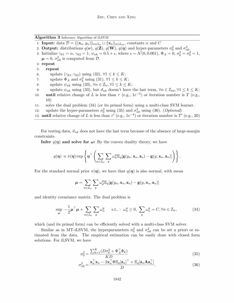
Zhu, Chen and Xing
Algorithm 3 Inference Algorithm of iLSVM
1: Input: data D = (xn, yn)n∈Itr ∪ xnn∈Itst , constants α and C2: Output: distributions q(ν), q(Z), q(W), q(η) and hyper-parameters σ2
0 and σ2n0
3: Initialize γk1 = α, γk2 = 1, ψnk = 0.5 + ε, where ε ∼ N (0, 0.001), Φ.k = 0, σ2k = σ2
0 = 1,µ = 0, σ2
n0 is computed from D.4: repeat5: repeat6: update (γk1, γk2) using (32), ∀1 ≤ k ≤ K;7: update Φ.k and σ2
k using (31), ∀1 ≤ k ≤ K;8: update ψnk using (33), ∀n ∈ Itr, ∀1 ≤ k ≤ K;9: update ψnk using (33), but ϑnk doesn’t have the last term, ∀n ∈ Itst,∀1 ≤ k ≤ K;
10: until relative change of L is less than τ (e.g., 1e−3) or iteration number is T (e.g.,10)
11: solve the dual problem (34) (or its primal form) using a multi-class SVM learner.12: update the hyper-parameters σ2
0 using (35) and σ2n0 using (36). (Optional)
13: until relative change of L is less than τ ′ (e.g., 1e−4) or iteration number is T ′ (e.g., 20)
For testing data, ϑnk does not have the last term because of the absence of large-marginconstraints.
Infer q(η) and solve for ω: By the convex duality theory, we have
q(η) ∝ π(η) exp
η>
(∑n∈Itr
∑y
ωynEq[g(yn,xn, zn)− g(y,xn, zn)]
).
For the standard normal prior π(η), we have that q(η) is also normal, with mean
µ =∑n∈Itr
∑y
ωydEq[g(yn,xn, zn)− g(y,xn, zn)]
and identity covariance matrix. The dual problem is
supω−1
2µ>µ+
∑n∈Itr
∑y
ωyn s.t.. : ωyn ≥ 0,∑y
ωyn = C,∀n ∈ Itr, (34)
which (and its primal form) can be efficiently solved with a multi-class SVM solver.
Similar as in MT-iLSVM, the hyperparameters σ20 and σ2
n0 can be set a priori or es-timated from the data. The empirical estimation can be easily done with closed formsolutions. For iLSVM, we have
σ20 =
∑Kk=1(Dσ2
k + Φ>.kΦk)
KD(35)
σ2n0 =
x>nxn − 2x>nΦEp[zn]> + Eq[znAz>n ]
D. (36)
1842

Regularized Bayesian Inference and Infinite Latent SVMs
References
Yasemin Altun and Alex Smola. Unifying divergence minimization and statistical inferencevia convex duality. In International Conference on Learning Theory, pages 139–153, 2006.
Rie Kubota Ando and Tong Zhang. A framework for learning predictive structures frommultiple tasks and unlabeled data. Journal of Machine Learning Research, (6):1817–1853,2005.
Charles E. Antoniak. Mixture of Dirichlet process with applications to Bayesian nonpara-metric problems. Annals of Statistics, (273):1152–1174, 1974.
Andreas Argyriou, Theodoros Evgeniou, and Massimiliano Pontil. Multi-task feature learn-ing. In Advances in Neural Information Processing Systems, pages 41–48, 2007.
Bart Bakker and Tom Heskes. Task clustering and gating for Bayesian multitask learning.Journal of Machine Learning Research, (4):83–99, 2003.
Andrew Barron, Mark Schervish, and Larry Wasserman. The consistency of posteriordistributions in nonparametric problems. The Annals of Statistics, 27(2):536–561, 1999.
Matthew J. Beal, Zoubin Ghahramani, and Carl E. Rasmussen. The infinite hidden Markovmodel. In Advances in Neural Information Processing Systems, pages 577–584, 2002.
Kedar Bellare, Gregory Druck, and Andrew McCallum. Alternating projections for learningwith expectation constraints. In Uncertainty in Artificial Intelligence, 2009.
David Blei and Peter Frazier. Distance dependent Chinese restaurant process. In Interna-tional Conference on Machine Learning, pages 87–94, 2010.
David Blei, Andrew Ng, and Michael I. Jordan. Latent Dirichlet allocation. Journal ofMachine Learning Research, (3):993–1022, 2003.
Edwin Bonilla, Kian Ming Chai, and Christopher Williams. Multi-task Gaussian processprediction. In Advances in Neural Information Processing Systems, pages 153–160, 2008.
Jonathan Borwein and Qiji Zhu. Techniques of Variational Analysis: An Introduction.Springer, New York, NY, 2005.
Stephen Boyd and Lieven Vandenberghe. Convex Optimization. Cambridge UniversityPress, 2004.
Ming-Wei Chang, Lev Ratinov, and Dan Roth. Guiding semi-supervision with constraint-driven learning. In the 45th Annual Meeting of the Association of Computational Lin-guistics, pages 280–287, 2007.
Ning Chen, Jun Zhu, Fuchun Sun, and Eric P. Xing. Large-margin predictive latent subspacelearning for multiview data analysis. IEEE Trans. on Pattern Analysis and MachineIntelligence (TPAMI), 34(12):2365–2378, 2012.
1843

Zhu, Chen and Xing
Ning Chen, Jun Zhu, Fuchun Sun, and Bo Zhang. Learning harmonium models with infinitelatent features. IEEE Transactions on Neural Networks and Learning Systems, 25(3):520–532, 2014.
Taeryon Choi and R. V. Ramamoorthi. Remarks on consistency of posterior distributions.IMS Collections 3. Pushing the limits of contemporary statistics: Contributions in honorof Jayanta K. Ghosh. eds. S. Ghosal and B. Clarke, pages 170–186, 2008.
Arthur P. Dempster, Nan M. Laird, and Donald B. Rubin. Maximum likelihood fromincomplete data via the EM algorithm. Journal of the Royal Statistical Society. SeriesB, 39(1):1–38, 1977.
Finale Doshi-Velez. The Indian buffet process: Scalable inference and extensions. Master’sthesis, The University of Cambridge, Aug 2009.
Mirosla Dudık, Steven J. Phillips, and Robert E. Schapire. Maximum entropy density esti-mation with generalized regularization and an application to species distribution model-ing. Journal of Machine Learning Research, (8):1217–1260, 2007.
David Dunson and Shyamal Peddada. Bayesian nonparametric inferences on stochasticordering. ISDS Discussion Paper, 2, 2007.
Thomas Ferguson. A Bayesian analysis of some nonparametric problems. Annals of Statis-tics, 1(2):209–230, 1973.
Morten Frydenberg. The chain graph Markov property. Scandinavian Journal of Statistics,17:333–353, 1990.
Kuzman Ganchev, Joao. Graca, Jennifer Gillenwater, and Ben Taskar. Posterior regular-ization for structured latent variable models. Journal of Machine Learning Research,(11):2001–2094, 2010.
Paul Garthwaite, Joseph Kadane, and Anthony O’Hagan. Statistical methods for elicitingprobability distributions. Journal of the American Statistical Association, 100(470):680–700, 2005.
Jayanta K. Ghosh and R.V. Ramamoorthi. Bayesian Nonparametrics. Springer, New York,NY, 2003.
Joao Graca, Kuzman Ganchev, and Ben Taskar. Expectation maximization and posteriorconstraints. In Advances in Neural Information Processing Systems, pages 569–576, 2007.
Thomas Griffiths and Zoubin Ghahramani. Infinite latent feature models and the Indianbuffet process. Technical report, University College London, GCNU TR2005-001, 2005.
Thomas L. Griffiths and Mark Steyvers. Finding scientific topics. Proceedings of the NationalAcademy of Sciences, 101:5228–5235, 2004.
Peter D. Hoff. Bayesian methods for partial stochastic orderings. Biometrika, 90:303–317,2003.
1844
Regularized Bayesian Inference and Infinite Latent SVMs
Seungil Huh and Stephen Fienberg. Discriminative topic modeling based on manifold learn-ing. ACM Transactions on Knowledge Discovery from Data, 5(4), 2012.
Kazufumi Ito and Karl Kunisch. Lagrange Multiplier Approach to Variational Problemsand Applications. Advances in Design and Control, Society for Industrial and AppliedMathematics (SIAM), Philadelphia, PA, 2008.
Tommi Jaakkola, Meila Meila, and Tony Jebara. Maximum entropy discrimination. InAdvances in Neural Information Processing Systems, pages 470–476, 1999.
Tony Jebara. Discriminative, Generative and Imitative Learning. PhD thesis, Media Lab-oratory, MIT, Dec 2001.
Tony Jebara. Multitask sparsity via maximum entropy discrimination. Journal of MachineLearning Research, (12):75–110, 2011.
Qixia Jiang, Jun Zhu, Maosong Sun, and Eric P. Xing. Monte Carlo methods for maximummargin supervised topic models. In Advances in Neural Information Processing Systems,pages 1592–1600, 2012.
Thorsten Joachims. Transductive inference for text classification using support vector ma-chines. In International Conference on Machine Learning, 1999.
Michael I. Jordan, Zoubin Ghahramani, Tommis Jaakkola, and Lawrence K. Saul. Anintroduction to variational methods for graphical models. Machine Learning, 37:183–233,1999.
Mohammad E. Khan, Guillaume Bouchard, Benjamin Marlin, and Kevin Murphy. Varia-tional bounds for mixed-data factor analysis. In Advances in Neural Information Pro-cessing Systems, pages 1108–1116, 2010.
John Lafferty, Andrew McCallum, and Fernando Pereira. Conditional random fields: Prob-abilistic models for segmenting and labeling sequence data. In International Conferenceon Machine Learning, pages 282–289, 2001.
Percy Liang, Michael I. Jordan, and Dan Klein. Learning from measurements in exponentialfamilies. In International Conference on Machine Learning, pages 641–648, 2009.
Steven N. MacEachern. Dependent nonparametric process. In the Section on BayesianStatistical Science of ASA, 1999.
Thomas L. Magnanti. Fenchel and Lagrange duality are equivalent. Mathematical Program-ming, (7):253–258, 1974.
Gideon Mann and Andrew McCallum. Generalized expectation criteria for semi-supervisedlearning with weakly labeled data. Journal of Machine Learning Research, (11):955–984,2010.
Shike Mei, Jun Zhu, and Xiaojin Zhu. Robust RegBayes: Selectively incorporating first-order logic domain knowledge into bayesian models. In International Conference onMachine Learning, pages 253–261, 2014.
1845

Zhu, Chen and Xing
Kurt Miller, Thomas Griffiths, and Michael I. Jordan. Nonparametric latent feature modelsfor link prediction. In Advances in Neural Information Processing Systems, pages 1276–1284, 2009.
Iain Murray and Zoubin Ghahramani. Bayesian learning in undirected graphical models:Approximate MCMC algorithms. In Uncertainty in Artificial Intelligence, 2004.
Peter Orbanz. Nonparametric priors on complete separable metric spaces. Working paper,2012.
Yuan (Alan) Qi, Martin Szummer, and Thomas P. Minka. Bayesian conditional randomfields. In International Conference on Artificial Intelligence and Statistics, pages 269–276,2005.
Piyush Rai and Hal Daume III. Infinite predictor subspace models for multitask learning.In International Conference on Artificial Intelligence and Statistics, pages 613–620, 2010.
Charles E. Rasmussen and Zoubin Ghahramani. Infinite mixtures of Gaussian processexperts. In Advances in Neural Information Processing Systems, pages 881–888, 2002.
Christian P. Robert. Simulation of truncated normal variables. Statistics and Computing,5(2):121–125, 1995.
Edward Schofield. Fitting maximum-entropy models on large sample spaces. PhD thesis,PhD thesis, Department of Computing, Imperial College London, 2006.
Wolfgang Stummer and Igor Vajda. On bregman distances and divergences of probabilitymeasures. IEEE Trans. on Information Theory, 58(3):1277–1288, 2012.
Ben Taskar, Carlos Guestrin, and Daphne Koller. Max-margin Markov networks. In Ad-vances in Neural Information Processing Systems, 2003.
Yee Whye Teh, Dilan Gorur, and Zoubin Ghahramani. Stick-breaking construction of theIndian buffet process. In International Conference on Artificial Intelligence and Statistics,pages 556–563, 2007.
Yee Whye Teh, Michael I. Jordan, Matthew J. Beal, and David Blei. Hierarchical Dirichletprocess. Journal of the American Statistical Association, 101(476):1566–1581, 2006.
Romain Thibaux and Michael I. Jordan. Hierarchical Beta processes and the Indian buffetprocess. In International Conference on Artificial Intelligence and Statistics, pages 564–571, 2007.
Vladimir Vapnik. The Nature of Statistical Learning Theory. Springer, New York, 1995.
Martin Wainright and Michael I. Jordan. Graphical models, exponential family, and varia-tional methods. Foundations and Trends in Machine Learning, 1(1):1–305, 2008.
Max Welling and Sridevi Parise. Bayesian random fields: The Bethe-Laplace approximation.In Uncertainty in Artificial Intelligence, 2006.
1846

Regularized Bayesian Inference and Infinite Latent SVMs
Max Welling, Ian Porteous, and Kenichi Kurihara. Exchangeable inconsistent priors forBayesian posterior inference. In Workshop on Information Theory and Applications,2012.
Max Welling, M. Rosen-Zvi, and G. Hinton. Exponential family harmoniums with an appli-cation to information retrieval. In Advances in Neural Information Processing Systems,pages 1481–1488, 2004.
Peter M. Williams. Bayesian conditionalisation and the principle of minimum information.The British Journal for the Philosophy of Science, 31(2), 1980.
Sinead Williamson, Peter Orbanz, and Zoubin Ghahramani. Dependent Indian buffet pro-cesses. In International Conference on Artifficial Intelligence and Statistics, pages 924–931, 2010.
Minjie Xu, Jun Zhu, and Bo Zhang. Bayesian nonparametric max-margin matrix factoriza-tion for collaborative prediction. In Advances in Neural Information Processing Systems,pages 64–72, 2012.
Ya Xue, David Dunson, and Lawrence Carin. The matrix stick-breaking process for flexiblemulti-task learning. In International Conference on Machine Learning, pages 1063–1070,2007.
Yu Zhang and Dit-Yan Yeung. A convex formulation for learning task relationships inmulti-task learning. In Uncertainty in Artificial Intelligence, 2010.
Jun Zhu. Max-margin nonparametric latent feature relational models for link prediction.In International Conference on Machine Learning, pages 719–726, 2012.
Jun Zhu, Amir Ahmed, and Eric P. Xing. MedLDA: Maximum margin supervised topicmodels for regression and classification. In International Conference on Machine Learn-ing, pages 1257–1264, 2009.
Jun Zhu, Ning Chen, Hugh Perkins, and Bo Zhang. Gibbs max-margin topic models withfast inference algorithms. In International Conference on Machine Learning, pages 124–132, 2013.
Jun Zhu, Ning Chen, and Eric P. Xing. Infinite latent SVM for classification and multi-task learning. In Advances in Neural Information Processing Systems, pages 1620–1628,2011a.
Jun Zhu, Ning Chen, and Eric P. Xing. Infinite SVM: a Dirichlet process mixture oflarge-margin kernel machines. In International Conference on Machine Learning, pages617–624, 2011b.
Jun Zhu and Eric P. Xing. Maximum entropy discrimination Markov networks. Journal ofMachine Learning Research, (10):2531–2569, 2009.
1847