Bayesian Learning in Social Networks - NYUpages.stern.nyu.edu/~ilobel/socialnetworks_revised.pdf · BAYESIAN LEARNING IN SOCIAL NETWORKS 1203 orseveralagentsrandomlydrawnfromtheentireortherecentpast.Ourrepresentationalsodoes

“rdr004” — 2011/10/17 — 7:35 — page 1201 — #1

Review of Economic Studies (2011) 78, 1201–1236 doi: 10.1093/restud/rdr004© The Author 2011. Published by Oxford University Press on behalf of The Review of Economic Studies Limited.Advance access publication 7 March 2011

Bayesian Learning in SocialNetworks

DARON ACEMOGLU and MUNTHER A. DAHLEHMassachusetts Institute of Technology

ILAN LOBELNew York University

andASUMAN OZDAGLAR

Massachusetts Institute of Technology

First version received November 2008; final version accepted December 2010 (Eds.)

We study the (perfect Bayesian) equilibrium of a sequential learning model over a general socialnetwork. Each individual receives a signal about the underlying state of the world, observes the past ac-tions of a stochastically generated neighbourhood of individuals, and chooses one of two possible actions.The stochastic process generating the neighbourhoods defines the network topology. We characterize purestrategy equilibria for arbitrary stochastic and deterministic social networks and characterize the condi-tions under which there will be asymptotic learning—convergence (in probability) to the right action asthe social network becomes large. We show that when private beliefs are unbounded (meaning that theimplied likelihood ratios are unbounded), there will be asymptotic learning as long as there is some min-imal amount of “expansion in observations”. We also characterize conditions under which there will beasymptotic learning when private beliefs are bounded.

Key words: Information aggregation, Learning, Social networks, Herding, Information cascades

JEL Codes: C72, D83

1. INTRODUCTION

How is dispersed and decentralized information held by a large number of individuals aggre-gated? Imagine a situation in which each of a large number of individuals has a noisy signalabout an underlying state of the world. This state of the world might concern, among otherthings, earning opportunities in a certain occupation, the quality of a new product, the suitabilityof a particular political candidate for office or pay-off-relevant actions taken by the government.If signals are unbiased, the combination—aggregation—of the information of the individualswill be sufficient for the society to “learn” the true underlying state. The above question can beformulated as the investigation of what types of behaviours and communication structures willlead to this type of information aggregation.Condorcet’s Jury theorem provides a natural benchmark, where sincere (truthful) reporting

of their information by each individual is sufficient for aggregation of information by a law oflarge numbers argument (Condorcet, 1785). Against this background, a number of papers, most

1201

“rdr004” — 2011/10/17 — 7:35 — page 1202 — #2

1202 REVIEW OF ECONOMIC STUDIES

notably Bikhchandani, Hirshleifer and Welch (1992), Banerjee (1992), and Smith and Sorensen(2000), show how this type of aggregation might fail in the context of the (perfect) Bayesianequilibrium of a dynamic game: when individuals act sequentially and observe the actions ofall previous individuals (agents), there may be “herding” on the wrong action, preventing theefficient aggregation of information.An important modelling assumption in these papers is that each individual observes all past

actions. In practice, individuals are situated in complex social networks, which provide theirmain source of information.1 In this paper, we address how the structure of social networks,which determines the information that individuals receive, affects equilibrium information ag-gregation in a sequential learning environment.As a motivating example, consider a group of consumers deciding which one of two possi-

ble new smartphones to switch to. Each consumer makes this decision when her existing ser-vice contract expires, so that there is an exogenous sequence of actions determined by contractexpiration dates. Each consumer observes the choices of some of her friends, neighbours andcoworkers, and the approximate timing of these choices (as she sees when they start using thenew phone). She does not, however, observe who else these friends, neighbours, and coworkershave themselves observed. Additional information from direct communication is limited sinceconsumers cannot easily identify and communicate their valuations soon after a new purchase.A related example would be the choice of a firm between two new technologies after the (ex-ogenous) breakdown of its current technology. The firm observes the nature and timing of thechoices of some of the nearby firms, but not what other information these firms had at the timethey made their decisions. In this case also, the main source of information would be observationof past actions rather than direct communication.Similar to these examples, in our model, a large number of agents sequentially choose be-

tween two actions. An underlying state determines the pay-offs of these two actions. Each agentreceives a signal on which of these two actions yield a higher pay-off. Preferences of all agentsare aligned in the sense that, given the underlying state of the world, they all prefer the same ac-tion. In addition to his own signal, each agent observes the choices of others in a stochasticallygenerated neighbourhood. In line with the examples above, each individual knows the identityof the agents in his neighbourhood. But he does not observe their private signal or necessarilyknow what information these agents had access to when making their own decisions.More formally, this dynamic game of incomplete information is characterized by two fea-

tures: (1) the signal structure, which determines how informative the signals received by theindividuals are and (2) the (social) network topology. We represent the network topology bya sequence of probability distributions (one for each agent) over subsets of past actions. Theenvironment most commonly studied in the previous literature, the full observation networktopology, is the special case where all past actions are observed. Another deterministic specialcase is the network topology where each agent observes the actions of the most recent M ≥ 1individuals. Other relevant networks include stochastic topologies in which each agent observesa random subset of past actions, as well as those in which, with a high probability, each agentobserves the actions of some “influential” group of agents, who may be thought of as “informa-tional leaders” or the media. In addition to these examples, our representation of social networksis sufficiently general to nest several commonly studied models of stochastic networks, includingsmall-world models, and observation structures in which each individual sees the actions of one

1. Granovetter (1973), Montgomery (1991), Munshi (2003), and Ioannides and Loury (2004) document the im-portance of information obtained from the social network of an individual for employment outcomes. Besley and Case(1994), Foster and Rosenzweig (1995), Munshi (2004), and Udry and Conley (2001) show the importance of the infor-mation obtained from social networks for technology adoption. Jackson (2006, 2007) provides excellent surveys.

“rdr004” — 2011/10/17 — 7:35 — page 1203 — #3

ACEMOGLU ET AL. BAYESIAN LEARNING IN SOCIAL NETWORKS 1203

or several agents randomly drawn from the entire or the recent past. Our representation also doesnot impose any restriction on the degree distribution (cardinality) of the agents’ neighbourhoodsor the degree of clustering in the network.We provide a systematic characterization of the conditions under which there will be asymp-

totic learning in this model. We say that there is asymptotic learning if as the size of the societybecomes arbitrarily large, equilibrium actions converge (in probability) to the action that yieldsthe higher pay-off. Conversely, asymptotic learning fails if, as the society becomes large, thecorrect action is not chosen (or more formally, the liminf of the probability that the right actionis chosen is strictly less than 1).Two concepts turn out to be central in the study of sequential learning in social networks. The

first is whether the likelihood ratio implied by individual signals is always finite and boundedaway from 0.2 Smith and Sorensen (2000) refer to beliefs that satisfy this property as bounded(private) beliefs. With bounded beliefs, there is a maximum amount of information in any indi-vidual signal. In contrast, when there exist signals with arbitrarily high and low likelihood ratios,(private) beliefs are unbounded. Whether bounded or unbounded beliefs provide a better approx-imation to reality is partly an interpretational and partly an empirical question. The main resultof Smith and Sorensen is that when each individual observes all past actions and private beliefsare unbounded, information will be aggregated and the correct action will be chosen asymptot-ically. In contrast, the results in Bikhchandani, Hirshleifer and Welch (1992), Banerjee (1992),and Smith and Sorensen (2000) indicate that with bounded beliefs, there will not be asymptoticlearning (or information aggregation). Instead, as emphasized by Bikhchandani, Hirshleifer andWelch (1992) and Banerjee (1992), there will be “herding” or “informational cascades”, whereindividuals copy past actions and/or completely ignore their own signals.The second key concept is that of a network topology with expanding observations. To de-

scribe this concept, let us first introduce another notion: a finite group of agents is excessivelyinfluential if there exists an infinite number of agents who, with probability uniformly boundedaway from 0, observe only the actions of a subset of this group. For example, a group is exces-sively influential if it is the source of all information (except individual signals) for an infinitelylarge component of the social network. If there exists an excessively influential group of individ-uals, then the social network has non-expanding observations, and conversely, if there exists noexcessively influential group, the network has expanding observations. This definition impliesthat most reasonable social networks have expanding observations, and in particular, a minimumamount of “arrival of new information ” in the social network is sufficient for the expanding ob-servations property.3 For example, the environment studied in most of the previous work in thisarea, where all past actions are observed, has expanding observations. Similarly, a social networkin which each individual observes one uniformly drawn individual from those who have takendecisions in the past or a network in which each individual observes her immediate neighbour allfeature expanding observations. A simple, but typical, example of a network with non-expandingobservations is the one in which all future individuals only observe the actions of the first K < ∞agents.Our main results in this paper are presented in four theorems. In particular, Theorems 2

and 4 are the most substantive contributions of this paper. Theorem 1 shows that there is noasymptotic learning in networks with non-expanding observations. This result is not surprisingsince information aggregation is not possible when the set of observations on which (an infinitesubset of) individuals can build their decisions remains limited forever.

2. The likelihood ratio is the ratio of the probabilities or the densities of a signal in one state relative to the other.3. Here, “arrival of new information” refers to the property that the probability of each individual observing the

action of some individual from the recent past converges to one as the social network becomes arbitrarily large.

“rdr004” — 2011/10/17 — 7:35 — page 1204 — #4


Theorem 2 shows that when (private) beliefs are unbounded and the network topology isexpanding, there will be asymptotic learning. This is a strong result (particularly if we considerunbounded beliefs to be a better approximation to reality than bounded beliefs) since almostall reasonable social networks have the expanding observations property. This theorem, e.g.implies that when some individuals, such as “informational leaders”, are overrepresented in theneighbourhoods of future agents (and are thus “influential”, though not excessively so), learningmay slow down, but asymptotic learning will still obtain as long as private beliefs are unbounded.Theorem 3 presents a partial converse to Theorem 2. It shows that for many common de-

terministic and stochastic networks, bounded private beliefs are incompatible with asymptoticlearning. It therefore generalizes existing results on asymptotic learning, e.g. those inBikhchandani, Hirshleifer and Welch (1992), Banerjee (1992), and Smith and Sorensen (2000),to general networks.Our final main result, Theorem 4, establishes that there is asymptotic learning with bounded

private beliefs for a sizable class of stochastic network topologies. Suppose there exists a subsetS of the agents such that agents in S have probability ε > 0 of observing the entire history ofactions and that an infinite subset of the agents in S makes decisions (partially) based on theirprivate signals because they have neighbours whose actions are not completely informative. Theremaining agents in the society have expanding observations with respect to S (in the sense thatthey are likely to observe some recent actions from S). Then, Theorem 4 shows that asymptoticlearning occurs for any distribution of private signals.This result is particularly important since it shows how moving away from simple network

structures, which have been the focus of prior work, has major implications for equilibriumlearning dynamics. In particular, the network structure that leads to asymptotic learning even inthe absence of strong signals is a combination of three features: (1) the presence of a set of agentsacting based on their private signals, (2) the presence of a different set of agents observing allactions who can thus piece together the state of the world from the actions of the agents that actaccording to their signals, and (3) a variant of expanding observations that ensures the existenceof information paths the agents that have access to the entire history of actions to most otheragents.Our paper contributes to the large and growing literature on social learning. Bikhchandani,

Hirshleifer and Welch (1992) and Banerjee (1992) started the literature on learning in situationsin which individuals are Bayesian and observe past actions. Smith and Sorensen (2000) providethe most comprehensive and complete analysis of this environment. Their results and the impor-tance of the concepts of bounded and unbounded beliefs, which they introduced, have alreadybeen discussed in the introduction and will play an important role in our analysis in the restof the paper. Other important contributions in this area include, among others, Welch (1992),Lee (1993), Chamley and Gale (1994), and Vives (1997). An excellent general discussion iscontained in Bikhchandani, Hirshleifer and Welch (1998). These papers typically focus on thespecial case of full observation network topology in terms of our general model.The two papers most closely related to ours are Banerjee and Fudenberg (2004) and Smith

and Sorensen (2008). Both of these papers study social learning with sampling of past actions.In Banerjee and Fudenberg, there is a continuum of agents and the focus is on proportionalsampling (whereby individuals observe a “representative” sample of the overall population).They establish that asymptotic learning is achieved under mild assumptions as long as the samplesize is no smaller than two. The existence of a continuum of agents is important for this resultsince it ensures that the fraction of individuals with different posteriors evolves deterministically.Smith and Sorensen, on the other hand, consider a related model with a countable number ofagents. In their model, as in ours, the evolution of beliefs is stochastic. Smith and Sorensenprovide conditions under which asymptotic learning takes place.

“rdr004” — 2011/10/17 — 7:35 — page 1205 — #5


A crucial difference between the study of Banerjee and Fudenberg and Smith and Sorensen,on the one hand, and our work, on the other, is the information structure. These papers assumethat “samples are unordered” in the sense that individuals do not know the identity of the agentsthey have observed. In contrast, as mentioned above, our setup is motivated by a social networkand assumes that individuals have stochastic neighbourhoods, but know the identity of the agentsin their realized neighbourhood. We view this as a better approximation to sequential learningin social networks. While situations in which an individual observes the actions of “strangers”would naturally correspond to “unordered samples”, in most social networks situations, individ-uals have some idea about where others are situated in the network. For example, an individualwould have some idea about which of their friends and coworkers are likely to have observedthe choices of many others, which in the context of our model corresponds to “ordered sam-ples”. In addition to its descriptive realism, this assumption leads to a sharper characterizationof the conditions under which asymptotic learning occurs. For example, in the environmentof Smith and Sorensen, asymptotic learning fails whenever an individual is “oversampled”, inthe sense of being overrepresented in the samples of future agents. In contrast, in our environ-ment, asymptotic learning occurs when the network topology features expanding observations(and private beliefs are unbounded). Expanding observations is a much weaker requirement than“non-oversampling”. For example, when each individual observes Agent 1 and a randomly cho-sen agent from his predecessors, the network topology satisfies expanding observations, but thereis oversampling.4Other recent work on social learning includes Celen and Kariv (2004), who study Bayesian

learning when each individual observes his immediate predecessor, Callander and Horner (2009),who show that it may be optimal to follow the actions of agents that deviate from past averagebehaviour, and Gale and Kariv (2003), who generalize the pay-off equalization result of Balaand Goyal (1998) in connected social networks (discussed below) to Bayesian learning.5The second branch of the literature focuses on non-Bayesian learning, typically with agents

using some reasonable rules of thumb. This literature considers both learning from past actionsand from pay-offs (or directly from beliefs). Early papers in this literature include Ellison andFudenberg (1993, 1995), which show how rule-of-thumb learning can converge to the true un-derlying state in some simple environments. The papers most closely related to our work in thisgenre are Bala and Goyal (1998, 2001), DeMarzo, Vayanos and Zwiebel (2003), and Golub andJackson (2010). These papers study non-Bayesian learning over an arbitrary connected socialnetwork. Bala and Goyal (1998) establish the important and intuitive pay-off equalization resultthat, asymptotically, each individual must receive a pay-off equal to that of an arbitrary individ-ual in his “social network” since otherwise he could copy the behaviour of this other individual.Our paper can be viewed as extending the results of Bala and Goyal to a sequential settingwith Bayesian learning. A similar “imitation” intuition plays an important role in our proof ofasymptotic learning with unbounded beliefs and unbounded observations. A key difference be-tween our results and those in the studies of Bala and Goyal; DeMarzo, Vayanos, and Zwiebel;and Golub and Jackson concerns the effects of “influential” groups on learning. In these non-Bayesian papers, an influential group or what Bala and Goyal refer to as a royal family, whichis highly connected to the rest of the network, prevents aggregation of information. In contrast,in our model, Bayesian updating ensures that such individuals do not receive disproportionate

4. This also implies that, in the terminology of Bala and Goyal, a “royal family” precludes learning in the modelof Smith and Sorensen, but as we show below, not in ours.

5. Gale and Kariv show that the behavior of agents in a connected social network who repeatedly act accordingto their posterior beliefs eventually converge. This does not constitute asymptotic learning according to our definitionsince behavior does not necessarily converge to the optimal action given the available information.

“rdr004” — 2011/10/17 — 7:35 — page 1206 — #6


weight and their presence does not preclude efficient aggregation of information. Only whenthere is an excessively influential group, i.e. a group that is the sole source of information for aninfinite subset of individuals, that asymptotic learning breaks down.6The rest of the paper is organized as follows. Section 2 introduces our model. Section 3 char-

acterizes the (pure strategy) perfect Bayesian equilibria and introduces the concepts of boundedand unbounded beliefs. Section 4 presents our main results, Theorems 1–4, and discusses someof their implications (as well as presenting a number of corollaries to facilitate interpretation).Section 5 concludes. Appendix A contains the main proofs, while the Appendix B in Supple-mentary Material contains additional results and omitted proofs.

2. MODEL

A countably infinite number of agents (individuals), indexed by n ∈ N, sequentially make asingle decision each. The pay-off of agent n depends on an underlying state of the world θ andhis decision. To simplify the notation and the exposition, we assume that both the underlyingstate and decisions are binary. In particular, the decision of agent n is denoted by xn ∈ {0,1} andthe underlying state is θ ∈ {0,1}. The pay-off of agent n is

un(xn,θ) ={1 if xn = θ,

0 if xn ̸= θ .

Again to simplify notation, we assume that both values of the underlying state are equally likely,so that P(θ = 0) = P(θ = 1) = 1/2.The state θ is unknown. Each agent n ∈N forms beliefs about this state from a private signal

sn ∈ S (where S is a metric space or simply a Euclidean space) and from his observation of theactions of other agents. Conditional on the state of the world θ , the signals are independentlygenerated according to a probability measure Fθ . We refer to the pair of measures (F0,F1) as thesignal structure of the model. We assume that F0 and F1 are absolutely continuous with respectto each other, which immediately implies that no signal is fully revealing about the underlyingstate. We also assume that F0 and F1 are not identical, so that some signals are informative.These two assumptions on the signal structure are maintained throughout the paper and will notbe stated in the theorems explicitly.In contrast to much of the literature on social learning, we assume that agents do not neces-

sarily observe all previous actions. Instead, they observe the actions of other agents accordingto the structure of the social network. To introduce the notion of a social network, let us firstdefine a neighbourhood. Each agent n observes the decisions of the agents in his (stochasticallygenerated) neighbourhood, denoted by B(n).7 Since agents can only observe actions taken previ-ously, B(n) ⊆ {1,2, . . .,n−1}. Each neighbourhood B(n) is generated according to an arbitraryprobability distribution Qn over the set of all subsets of {1,2, . . .,n−1}. We impose no specialassumptions on the sequence of distributions {Qn}n∈N except that the draws from each Qn areindependent from each other for all n and from the realizations of private signals. The sequence{Qn}n∈N is the network topology of the social network formed by the agents. The network topol-ogy is common knowledge, whereas the realized neighbourhood B(n) and the private signal sn

6. There is also a literature in engineering, which studies related problems, especially motivated by aggregationof information collected by decentralized sensors. These include Cover (1969), Papastavrou and Athans (1992), Lorenz,Marciniszyn and Steger (2007), and Tay, Tsitsiklis and Win (2008). The work by Papastavrou and Athans contains aresult that is equivalent to the characterization of asymptotic learning with the observation of the immediate neighbour.

7. If n′ ∈ B(n), then agent n not only observes the action of n′ but also knows the identity of this agent. Crucially,however, n does not observe B(n′) or the actions of the agents in B(n′).

“rdr004” — 2011/10/17 — 7:35 — page 1207 — #7


are the private information of agent n. We say that {Qn}n∈N is a deterministic network topologyif the probability distribution Qn is a degenerate (Dirac) distribution for all n. Otherwise, i.e. if{Qn} for some n is non-degenerate, {Qn}n∈N is a stochastic network topology.A social network consists of a network topology {Qn}n∈N and a signal structure (F0,F1).

Example 1. Here are some examples of network topologies.

1. If {Qn}n∈N assigns probability 1 to neighbourhood {1,2, . . .,n−1} for each n ∈ N, then thenetwork topology is identical to the canonical one studied in the previous literature whereeach agent observes all previous actions (e.g. Banerjee, 1992; Bikhchandani, Hirshleiferand Welch, 1992; Smith and Sorensen, 2000).

2. If {Qn}n∈N assigns probability 1/(n−1) to each one of the subsets of size 1 of {1,2, . . .,n−1} for each n ∈ N, then we have a network topology of random sampling of one agent fromthe past.

3. If {Qn}n∈N assigns probability 1 to neighbourhood {n−1} for each n ∈ N, then we havea network topology where each individual only observes his immediate neighbour.

4. If {Qn}n∈N assigns probability 1 to neighbourhoods that are subsets of {1,2, . . .,K } foreach n ∈ N for some K ∈ N. In this case, all agents observe the actions of at most Kagents.

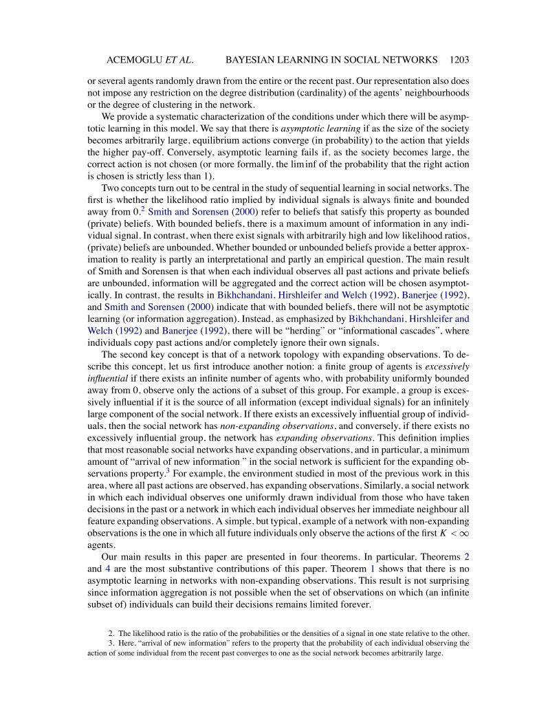
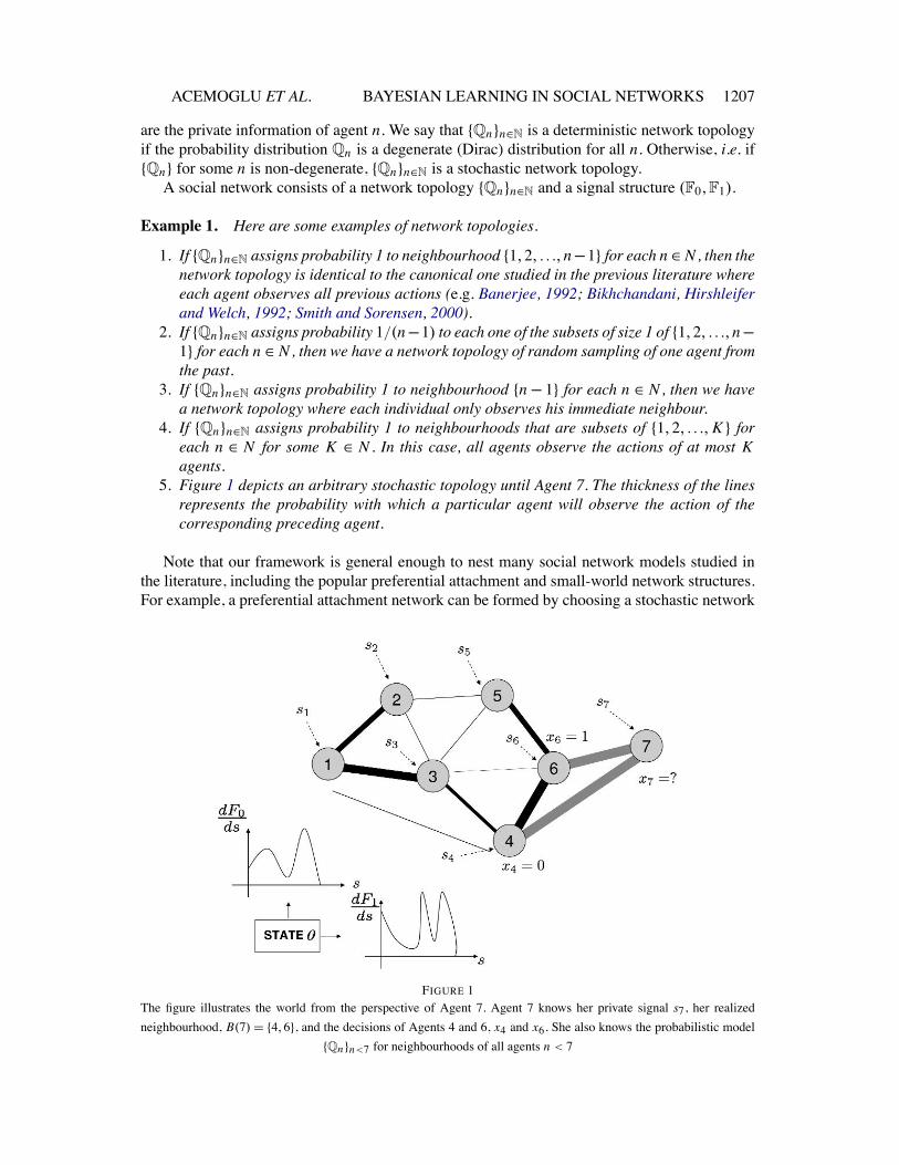
5. Figure 1 depicts an arbitrary stochastic topology until Agent 7. The thickness of the linesrepresents the probability with which a particular agent will observe the action of thecorresponding preceding agent.

Note that our framework is general enough to nest many social network models studied inthe literature, including the popular preferential attachment and small-world network structures.For example, a preferential attachment network can be formed by choosing a stochastic network

FIGURE 1The figure illustrates the world from the perspective of Agent 7. Agent 7 knows her private signal s7, her realizedneighbourhood, B(7) = {4,6}, and the decisions of Agents 4 and 6, x4 and x6. She also knows the probabilistic model

{Qn}n<7 for neighbourhoods of all agents n < 7

“rdr004” — 2011/10/17 — 7:35 — page 1208 — #8


topology {Qn}n∈N where all observations are independent of each other andQn(m ∈ B(n)) = αmfor a sequence of numbers {αm}m∈N. In this network, agents with a high α will be observed bymany peers, while agents with low α will not. A small-world network structure can be formedby choosing a partition {S j } of N such that for every m < n, the probability that m ∈ B(n) is highif both m and n belong to the set S j for some j and low, but positive, if both m and n belongto different sets S j and S j ′ . More generally, any network structure can be represented by a judi-cious choice of {Qn}n∈N provided that we keep the assumption that the realizations of {Qn}n∈Nare independent.8 The independence assumption on the neighbourhoods does not impose a re-striction on the degree distribution (cardinality) of the agents or on the degree of clustering ofthe agents. To observe this, note that any given deterministic network topology satisfies the in-dependence assumption and it can be selected to have an arbitrary degree distribution or level ofclustering.

3. EQUILIBRIUM STRATEGIES

In this section, we introduce the definitions of equilibrium and asymptotic learning and we pro-vide a characterization of equilibrium strategies. In particular, we show that equilibrium decisionrules of individuals can be decomposed into two parts, one that only depends on an individual’sprivate signal and the other that is a function of the observations of past actions. We also showwhy a full characterization of individual decisions is non-trivial and motivates an alternativeproof technique, relying on developing bounds on improvements in the probability of the cor-rect decisions, that will be used in the rest of our analysis.

3.1. Perfect Bayesian equilibrium and asymptotic learning

Given the description above, it is evident that the information set In of agent n is given by hersignal sn , her neighbourhood B(n), and all decisions of agents in B(n), i.e.

In = {sn, B(n), xk for all k ∈ B(n)}. (3.1)

The set of all possible information sets of agent n is denoted by In . The agent also knows thenetwork topology {Qn}n∈N, as it is common knowledge. A strategy for individual n is a mappingσn : In → {0,1} that selects a decision for each possible information set. A strategy profile is asequence of strategies σ = {σn}n∈N. We use the standard notation σ−n = {σ1, . . . ,σn−1,σn+1, . . .}to denote the strategies of all agents other than n and also (σn,σ−n) for any n to denote thestrategy profile σ . Given a strategy profile σ , the sequence of decisions {xn}n∈N is a stochasticprocess and we denote the measure generated by this stochastic process by Pσ .

Definition 1. A strategy profile σ is a pure strategy perfect Bayesian equilibrium of this gameof social learning if for each n ∈ N, σn maximizes the expected pay-off of agent n given thestrategies of other agents σ−n.

In the rest of the paper, we focus on pure strategy perfect Bayesian equilibria and simplyrefer to them as “equilibria” (without the pure strategy and the perfect Bayesian qualifiers). Werefer to the set of equilibria as %.

8. The independence assumption rules out generative preferential attachment models, such as Jackson and Rogers(2007), in which a particular individual being observed more frequently in the past increases the likelihood that he willbe observed in the future. Nevertheless, as noted in the text, networks with a preferential attachment structure can becast as special cases of our model, without abandoning the independence assumption, by fixing ex ante which agents aregoing be “highly connected”.

“rdr004” — 2011/10/17 — 7:35 — page 1209 — #9


Given a strategy profile σ , the expected pay-off of agent n from action xn = σn(In) is simplyPσ (xn = θ | In). Therefore, for any equilibrium σ , we have

σn(In) ∈ argmaxy∈{0,1}

P(y,σ ∗−n)(y = θ | In). (3.2)

We denote the set of equilibria (pure strategy perfect Bayesian equilibria) of the game by %. Itis clear that % is non-empty. Given the sequence of strategies {σ1, . . . ,σn−1}, the maximizationproblem in equation (3.2) has a solution for each agent n and each In ∈ In . Proceeding induc-tively, and choosing either one of the actions in case of indifference determines an equilibrium.We note the existence of equilibrium here.

Proposition 1. There exists a pure strategy perfect Bayesian equilibrium.

Our main focus is whether equilibrium behaviour will lead to information aggregation. Thisis captured by the notion of asymptotic learning, which is introduced next.

Definition 2. Given a signal structure (F0,F1) and a network topology {Qn}n∈N, we say thatasymptotic learning occurs in equilibrium σ if xn converges to θ in probability (according tomeasure Pσ ), i.e.

limn→∞Pσ (xn = θ) = 1.

Note that asymptotic learning requires that the probability of taking the correct action con-verges to 1.9 Therefore, asymptotic learning will fail when, as the network becomes large, thelimit inferior of the probability of all individuals taking the correct action is strictly less than 1.Our goal in this paper is to characterize conditions on social networks—on signal structures

and network topologies—that ensure asymptotic learning.

3.2. Characterization of individual decisions

Our first result shows that individual decisions can be characterized as a function of the sum oftwo posteriors. These posteriors play an important role in our analysis. We will refer to theseposteriors as the individual’s private belief and the social belief.

Proposition 2. Let σ ∈ % be an equilibrium of the game. Let In ∈ In be an information setof agent n. Then, the decision of agent n, xn = σn(In), satisfies

xn ={1, if Pσ (θ = 1 | sn)+Pσ (θ = 1 | B(n), xk,k ∈ B(n)) > 1,

0, if Pσ (θ = 1 | sn)+Pσ (θ = 1 | B(n), xk,k ∈ B(n)) < 1,

and xn ∈ {0,1} otherwise.

Proof. See Appendix A. ∥

This proposition establishes an additive decomposition in the equilibrium decision rule be-tween the information obtained from the private signal of the individual and from the obser-vations of others’ actions (in his neighbourhood). The next definition formally distinguishesbetween the two components of an individual’s information.

9. It is also clear that asymptotic learning is equivalent to the posterior beliefs converging to a distribution puttingprobability 1 on the true state.

“rdr004” — 2011/10/17 — 7:35 — page 1210 — #10


Definition 3. We refer to the probability Pσ (θ = 1 | sn), as the private belief of agent n,and the probability

Pσ (θ = 1 | B(n), xk for all k ∈ B(n)),

as the social belief of agent n.

Proposition 2 and Definition 3 imply that the equilibrium decision rule for agent n ∈ Nis equivalent to choosing xn = 1 when the sum of his private and social beliefs is greaterthan 1. Consequently, the properties of private and social beliefs will shape equilibrium learningbehaviour.Note that the social belief depends on n since it is a function of the (realized) neighbour-

hood of agent n. In most learning models, social beliefs have natural monotonicity properties.For example, a greater fraction of individuals choosing action x = 1 in the information set ofagent n would increase the social belief of agent n. It is straightforward to construct examples,where such monotonicity properties do not hold under general social networks (see Appendix Bin Supplementary Material). For this reason, we will use a different line of attack, based on de-veloping lower bounds on the probability of taking the correct action, for establishing our mainresults, which are presented in the next section.

3.3. Bounded and unbounded private beliefs

The private belief of an individual is a function of his private signal s ∈ S and is not a functionof the strategy profile σ since it does not depend on the decisions of other agents. We representprobabilities that do not depend on the strategy profile by P. We use the notation pn to representthe private belief of agent n, i.e.

pn = P(θ = 1 | sn).

A straightforward application of Bayes’ rule implies that for any n and any signal sn ∈ S, theprivate belief pn of agent n is given by10

pn =(1+ dF0

dF1(sn)

)−1. (3.3)

We next define the support of a private belief. In our subsequent analysis, we will see thatproperties of the support of private beliefs play a key role in asymptotic learning behaviour.Since the pn are identically distributed for all n (which follows by the assumption that the privatesignals sn are identically distributed), in the following, we will use Agent 1’s private belief p1to define the support and the conditional distributions of private beliefs.

Definition 4. The support of the private beliefs is the interval [β,β], where the end pointsof the interval are given by

β = inf{r ∈ [0,1] | P(p1 ≤ r) > 0} and β = sup{r ∈ [0,1] | P(p1 ≤ r) < 1}.

The signal structure has bounded private beliefs if β > 0 and β < 1 and unbounded privatebeliefs if β = 1−β = 1.

10. If the probability measures F0 and F1 have densities f0 and f1, respectively, thendF0dF1

(sn) = f0(sn )f1(sn ) .

“rdr004” — 2011/10/17 — 7:35 — page 1211 — #11


When private beliefs are bounded, there is a maximum informativeness to any signal. Whenthey are unbounded, agents may receive arbitrarily strong signals favouring either state (thisfollows from the assumption that (F0,F1) are absolutely continuous with respect to each other).The conditional distribution of private beliefs given the underlying state j ∈ {0,1} can be

directly computed asG j (r) = P(p1 ≤ r | θ = j). (3.4)

The signal structure (F0,F1) can be equivalently represented by the corresponding private beliefdistributions (G0,G1), and in what follows, it will typically be more convenient to work with(G0,G1) rather than (F0,F1). It is straightforward to verify that G0(r)/G1(r) is non-increasingin r and G0(r)/G1(r) > 1 for all r ∈ (β,β) (see Lemma A1 in Appendix A).

4. MAIN RESULTS

In this section, we present our main results on asymptotic learning and provide the main intuitionfor the proofs.

4.1. Expanding observations

We start by introducing the key properties of network topologies and signal structures that impactasymptotic learning. Intuitively, for asymptotic learning to occur, the information that each agentreceives from other agents should not be confined to a bounded subset of agents. This propertyis established in the following definition. For this definition and throughout the paper, if the setB(n) is empty, we set maxb∈B(n) b = 0.

Definition 5. The network topology has expanding observations if for all K ∈ N, we have

limn→∞Qn

(maxb∈B(n)

b < K)

= 0.

If the network topology does not satisfy this property, then we say it has non-expanding obser-vations.

Recall that the neighbourhood of agent n is a random variable B(n) (with values in theset of subsets of {1,2, . . .,n− 1}) and distributed according to Qn . Therefore, maxb∈B(n) b isa random variable that takes values in {0,1, . . .,n− 1}. The expanding observations conditioncan be restated as the sequence of random variables {maxb∈B(n) b}n∈N converging to infinity inprobability. Similarly, it follows from the preceding definition that the network topology hasnon-expanding observations if and only if there exists some K ∈ N and some scalar ε > 0 suchthat

limsupn→∞

Qn

(maxb∈B(n)

b < K)

≥ ε.

An alternative restatement of this definition might clarify its meaning. Let us refer to a finite setof individuals C as excessively influential if there exists a subsequence of agents who, with prob-ability uniformly bounded away from 0, observe the actions of a subset of C . Then, the networktopology has non-expanding observations if and only if there exists an excessively influentialgroup of agents. Note also that if there is a minimum amount of arrival of new information inthe network, so that the probability of an individual observing some other individual from therecent past goes to one as the network becomes large, then the network topology will featureexpanding observations. This discussion therefore highlights that the requirement that a network

“rdr004” — 2011/10/17 — 7:35 — page 1212 — #12


topology has expanding observations is quite mild and most social networks, including all ofthose discussed above, satisfy this requirement.When the topology has non-expanding observations, there is a subsequence of agents that

draws information from the first K decisions with positive probability (uniformly bounded awayfrom 0). It is then intuitive that network topologies with non-expanding observations will pre-clude asymptotic learning. Our first theorem states and proofs this result.

Theorem 1. Assume that the network topology {Qn}n∈N has non-expanding observations.Then, there exists no equilibrium σ ∈ % with asymptotic learning.


This theorem states the intuitive result that with non-expanding observations, asymptoticlearning will fail. This result is not surprising since asymptotic learning requires the aggregationof the information of different individuals. But a network topology with non-expanding observa-tions does not allow such aggregation. Intuitively, non-expanding observations, or equivalentlythe existence of an excessively influential group of agents, imply that infinitely many individu-als will observe finitely many actions with positive probability and this will not enable them toaggregate the dispersed information collectively held by the entire social network.

4.2. Asymptotic learning with unbounded private beliefs

A central question is then whether, once we exclude network topologies with non-expandingobservations, what other conditions need to be imposed to ensure asymptotic learning. The fol-lowing theorem is one of the main results of the paper and shows that for general networktopologies, unbounded private beliefs play a key role. In particular, unbounded private beliefsand expanding observations are sufficient for asymptotic learning in all equilibria.

Theorem 2. Assume that the signal structure (F0,F1) has unbounded private beliefs and thenetwork topology {Qn}n∈N has expanding observations. Then, asymptotic learning occurs inevery equilibrium σ ∈ %.


Theorem 2 implies that unbounded private beliefs are sufficient for asymptotic learning formost (but not all) network topologies. In particular, the condition that the network topology hasexpanding observations is fairly mild and only requires a minimum amount of arrival of recentinformation to the network. Social networks in which each individual observes all past actions,those in which each observes just his neighbour and those in which each individual observesM ≥ 1 agents independently and uniformly drawn from his predecessors are all examples ofnetwork topologies with expanding observations. Theorem 2 therefore implies that unboundedprivate beliefs are sufficient to guarantee asymptotic learning in social networks with these prop-erties and many others.This theorem also guarantees learning in the presence of agents who are highly influential, in

the sense that their actions are visible to the entire society, but are not excessively influential, asthey are not the only sources of information in the networks. Consider, e.g. a network where theactions of the first K agents are visible to everyone, but each agent also observes her immediateneighbour, i.e. B(n) = {1,2, . . .,K ,n− 1}. This network topology satisfies expanding observa-tions and thus leads to learning provided that private beliefs are unbounded. This is in contrast

“rdr004” — 2011/10/17 — 7:35 — page 1213 — #13


with the predictions of non-Bayesian learning models such as DeMarzo, Vayanos and Zwiebel(2003) and Golub and Jackson (2010). To see this, suppose, as in these models, that agents de-termine their new beliefs as a weighted average of their own beliefs and the beliefs of the agentsthey observe and that the first K agents are influential in the sense that they are observed by allfuture agents and receive a weight of at least ε > 0. It is then straightforward that there will notbe asymptotic learning, which contrasts with Theorem 2.The proof of Theorem 2 is presented in Appendix A. Here, we provide a road map and the

general intuition. As noted in the previous section, there is no monotonicity result linking thebehaviour of an agent to the fraction of actions he or she observes. Instead, we prove Theorem 2by making use of an informational monotonicity related to the (expected) welfare improvementprinciple in Banerjee and Fudenberg (2004) and in Smith and Sorensen (2008) and the imitationprinciple in Bala and Goyal (1998) and Gale and Kariv (2003). In particular, we first consider aspecial case in which each individual only observes one other from the past (i.e. B(n) is a single-ton for each n). We then establish the following strong improvement principle: with unboundedprivate beliefs, there exists a strict lower bound on the increase in the ex ante probability thatan individual will make a correct decision over his neighbour’s probability (recall that for nowthere is a single agent in each individual’s neighbourhood, thus each individual has a single“neighbour”). Intuitively, each individual can copy the behaviour of their neighbour unless theyhave a very strong signal that points in a different direction. We show that this results in a strictimprovement in the probability of taking the right action whenever this probability is not equalto 1.We then prove a generalized strong improvement principle for arbitrary social networks by

showing that each individual can obtain such an improvement even if they ignore all but one ofthe individuals in their information set. The overall improvement in the probability that each in-dividual will take the right action is a priori greater than this lower bound. The proof of Theorem2 then follows by using this generalized strong improvement principle to construct a subsequenceof informational improvements at each point and showing that there is a strict improvement ateach step of the subsequence. This combined with the expanding observations assumption onthe network topology establishes the asymptotic learning result in the proof of the theorem.The following corollary to Theorems 1 and 2 shows that for an interesting class of stochastic

network topologies, there is a critical topology at which there is a phase transition—i.e. forall network topologies with greater expansion of observations than this critical topology, therewill be asymptotic learning and for all topologies with less expansion, asymptotic learning willfail.

Corollary 1. Assume that the signal structure (F0,F1) has unbounded private beliefs. Assumealso that the network topology is given by {Qn}n∈N such that

Qn(m ∈ B(n)) = a(n−1)c f or all n and all m < n,

where, given n, the draws for m,m′ < n, are independent and a and c are positive constants. Ifc < 1, then asymptotic learning occurs in all equilibria. If c ≥ 1, then asymptotic learning doesnot occur in any equilibrium.


Given the class of network topologies in this corollary, c < 1 implies that as the networkbecomes large, there will be sufficient expansion of observations. In contrast, for c ≥ 1, stochas-tic process Qn does not place enough probability on observing recent actions and the network

“rdr004” — 2011/10/17 — 7:35 — page 1214 — #14


topology is non-expanding. Consequently, Theorem 1 applies and there is no asymptoticlearning.To highlight the implications of Theorems 1 and 2 for deterministic network topologies, let

us introduce the following definition.

Definition 6. Assume that the network topology is deterministic. Then, we say a finite sequenceof agents π is an information path of agent n if for each i , πi ∈ B(πi+1), and the last element ofπ is n. Let π(n) be an information path of agent n that has maximal length. Then, we let L(n)denote the number of elements in π(n) and call it agent n’s information depth.

Intuitively, the concepts of information path and information depth capture the intuitive no-tion of how long the “trail” of the information in the neighbourhood of an individual is. Forexample, if each individual observes only his immediate neighbour (i.e. B(n) = {n− 1} withprobability 1), each will have a small neighbourhood, but the information depth of a high-indexed individual will be high (or the “trail” will be long) because the immediate neighbour’saction will contain information about the signals of all previous individuals. The next corollaryshows that with deterministic network topologies, asymptotic learning will occur if and only ifthe information depth (or the trail of the information) increases without bound as the networkbecomes larger.

Corollary 2. Assume that the signal structure (F0,F1) has unbounded private beliefs. Assumethat the network topology is deterministic. Then, asymptotic learning occurs for all equilibria ifthe sequence of information depths {L(n)}n∈N goes to infinity. If the sequence {L(n)}n∈N doesnot go to infinity, then asymptotic learning does not occur in any equilibrium.


4.3. No learning under bounded private beliefs

In the full observation network topology, bounded beliefs imply lack of asymptotic learning.One might thus expect a converse to Theorem 2, whereby asymptotic learning fails wheneversignals are bounded. Under general network topologies, learning dynamics turn out to be moreinteresting and richer. The next theorem provides a partial converse to Theorem 2 and showsthat for a wide range of deterministic and stochastic network topologies, bounded beliefs implyno asymptotic learning. However, somewhat surprisingly, Theorem 4 will show that the same isnot true with more general stochastic network topologies.

Theorem 3. Assume that the signal structure (F0,F1) has bounded private beliefs. If thenetwork topology {Qn}n∈N satisfies one of the following conditions,

(a) B(n) = {1, . . . ,n−1} for all n,(b) |B(n)| ≤ 1 for all n, or(c) there exists some constant M such that |B(n)| ≤ M for all n and

limn→∞ max

b∈B(n)b = ∞ wi th probabili t y 1,

then, asymptotic learning does not occur in any equilibrium σ ∈ %.

Proof. See Appendix B in Supplementary Material. ∥

“rdr004” — 2011/10/17 — 7:35 — page 1215 — #15


This theorem implies that in many common deterministic and stochastic network topologies,bounded private beliefs imply lack of asymptotic learning. Part (a) of this theorem is alreadyproved by Smith and Sorensen (2000), we provide an alternative proof in Appendix B in Sup-plementary Material. Intuitively, in all cases, we can provide an upper bound on the amountof learning. We establish this upper bound by showing that either individuals start followingpotentially incorrect social beliefs after a certain stage of learning has been reached or they relyon their own private signal, taking the incorrect action with positive probability.Part (c) of the theorem is the more substantive contribution. The idea behind the proof of

Part (c) is as follows. We suppose, to obtain a contradiction, that asymptotic learning occurs. Wethen show that this implies that the social belief of agents who only observe neighbours selectingAction 1 converges to 1. The probability that the first K agents select Action 1 is positive (for anyK ). In case of such an event and K large, eventually all agents will have a social belief close to 1,which is proved using a union bound and the fact that each agent observes at most M actions.But since, with bounded private beliefs, an agent with social belief close to 1 will ignore hersignal, eventually decisions will contain no new information, contradicting asymptotic learning.The following corollary illustrates the implications of Theorem 3. It shows that, when private

beliefs are bounded, there will be no asymptotic learning (in any equilibrium) in stochasticnetworks with random sampling.

Corollary 3. Assume that the signal structure (F0,F1) has bounded private beliefs. Assumethat each agent n samples M agents uniformly and independently among {1, . . .,n−1} for someM ≥ 1. Then, asymptotic learning does not occur in any equilibrium σ ∈ %.


4.4. Asymptotic learning with bounded private beliefs

While in the full observation network topology studied by Smith and Sorensen (2000) and inother instances investigated in the previous literature, bounded private beliefs preclude asymp-totic learning, this is no longer true under general stochastic social networks. Characterizing theset of stochastic network topologies under which learning occurs for all distributions of privatebeliefs is the next major contribution of our paper. To present these results, we first introduce thenotion of a non-persuasive neighbourhood.

Definition 7. A finite set B ⊂ N is a non-persuasive neighbourhood in equilibrium σ ∈ % if

Pσ (θ = 1 | xk = yk for all k ∈ B) ∈ (1−β,1−β)

for any set of values yk ∈ {0,1} for each k. We denote the set of all non-persuasive neighbour-hoods by Uσ .

A neighbourhood B is non-persuasive in equilibrium σ ∈ % if for any set of decisions thatagent n observes, his behaviour may still depend on his private signal. That is, for any set of de-cisions the agent observes, there exists some private signal such that the agent chooses Action 0and some private signal such that the agent chooses Action 1.A non-persuasive neighbourhood is defined with respect to a particular equilibrium. How-

ever, we will provide below several different sufficient conditions for a collection of neighbour-hoods to be non-persuasive in any equilibrium.Our main theorem for learning with bounded beliefs provides a broad class of stochastic

social networks where asymptotic learning takes place for any signal structure. It relies on the

“rdr004” — 2011/10/17 — 7:35 — page 1216 — #16


society comprising two subsets, one learning from agents with non-persuasive neighbourhoodsand the other learning from the former subset. This necessitates strengthening the expandingobservations condition to ensure that the latter subset receives new information from the formersubset.

Definition 8. Given a subset S⊆N, the network topology {Qn}n∈N has expanding observationswith respect to S if for all K ,

limn→∞Qn

(max

b∈B(n)∩Sb < K

)= 0.

Theorem 4. Let (F0,F1) be an arbitrary signal structure and let S ⊆ N. Let σ be the equilib-rium where agents break ties in favour of Action 0.11 Assume the network topology {Qn}n∈N hasexpanding observations with respect to S and has a lower bound on the probability of observingthe entire history of actions along S, i.e. there exists some ε > 0 such that

Qn(B(n) = {1, . . .,n−1}) ≥ ε for all n ∈ S.

Assume further that for some positive integer M and non-persuasive neighbourhoods C1, . . .,CM, i.e. Ci ∈ Uσ for all i = 1, . . . ,M, we have

∑

n∈S

M∑

i=1Qn(B(n) = Ci ) = ∞.

Then, asymptotic learning occurs in equilibrium σ .


This is a rather surprising result, particularly in view of existing results in the literature,which generate herds and information cascades (and no learning) with bounded beliefs. Thistheorem indicates that learning dynamics become significantly richer when we consider generalsocial networks.Theorem 4 highlights a class of network structures that lead to learning. In these structures,

there is an infinite subset S that forms the core of the network. Within this core S, there are twoimportant subgroups of agents. There are infinitely many agents who act based (partially) ontheir signals since they have non-persuasive neighbourhoods. The existence of these agents doesnot preclude learning since the probability that an agent n has a non-persuasive neighbourhoodcan go to 0 as n goes to infinity. By acting based on their private signals, these agents playthe essential function of bringing new information into the society. The second key subgroupwithin the core of agents in S is the set of all agents who observe the entire history of play.These agents play the role of collecting the information brought in by the agents who have non-persuasive neighbourhoods. From the martingale convergence theorem, the social belief of theseagents converges with probability 1, and because there is sufficient information generated bythe agents with non-persuasive neighbourhoods, the social belief must converge to the correctstate of the world. The expanding observations with respect to S guarantees that informationspreads to all other agents. In particular, agents who do not observe the entire history of actions

11. This assumption is not necessary to prove this result but assuming a particular equilibrium significantly sim-plifies the notation needed in the proof.

“rdr004” — 2011/10/17 — 7:35 — page 1217 — #17


can simply copy the action of their highest neighbours within S. This strategy provides a lowerbound on the pay-off to these agents and in fact guarantees asymptotic learning. Therefore, theseagents also asymptotically learn the state in equilibrium.12We conclude this subsection by providing sufficient conditions for a neighbourhood to be

non-persuasive in any equilibrium. It is straightforward to see that B = ∅, i.e. the empty neigh-bourhood, is non-persuasive in any equilibrium. The following two propositions present twoother classes of non-persuasive neighbourhoods.

Proposition 3. Let (G0,G1) be private belief distributions. Assume that the first K agents haveempty neighbourhoods, i.e. B(n) = ∅ for all n ≤ K, and K satisfies

K <min

⎧⎨

⎩

log(

β1−β

)

log(G0(1/2)G1(1/2)

) ,log

(β

1−β

)

log(1−G0(1/2)1−G1(1/2)

)

⎫⎬

⎭ . (4.5)

Then, any subset B ⊆ {1,2, . . .,K } is a non-persuasive neighbourhood.


To obtain the intuition for equation (4.5), consider the equivalent pair of inequalities

(1+ G0(1/2)K

G1(1/2)K

)−1> 1−β and

(1+ (1−G0(1/2))K

(1−G1(1/2))K)−1

< 1−β. (4.6)

The factor of (1+ (G0(1/2)/G1(1/2))K )−1 represents the probability that the state θ is equalto 1 conditional on K agents independently selecting Action 0. For such a neighbourhood ofK agents acting independently to be non-persuasive, there must exist a signal strong enough infavour of State 1 such that an agent would select Action 1 after observing K independent agentschoosing 0. From the equilibrium decision rule (cf. Proposition 2), it follows that this holds if(1+ (G0(1/2)/G1(1/2))K )−1+β > 1. We can repeat the same argument for Action 1 to obtainthe second inequality in equation (4.6).The condition in equation (4.5) has a natural interpretation: for a neighbourhood B to be

non-persuasive, any |B| decisions have to be less informative than a single very informativesignal. In the case where an agent k ∈ B has an empty neighbourhood, the informativeness ofher decision xk = 0 is given by G0(1/2)/G1(1/2) and can be interpreted as the informativenessof an “average" signal in favour of State 0 since any signal mildly in favour of State 0 wouldlead to Action 0. Therefore, the ratio between the informative value of an average signal andthe informative value of an extreme signal determines the size |B| of the largest non-persuasiveneighbourhood.

12. It is important to emphasize the difference between this result and that in Sgroi (2002), which shows that asocial planner can ensure some degree of information aggregation by forcing a subsequence of agents to make decisionswithout observing past actions. With the same reasoning, one might conjecture that asymptotic learning may occur if aparticular subsequence of agents, such as that indexed by prime numbers, has empty neighbourhoods. However, therewill not be asymptotic learning in this deterministic topology since liminfn→∞Pσ (xn = θ) < 1. For the result thatthere is asymptotic learning (i.e. liminfn→∞Pσ (xn = θ) = 1) in Theorem 4, the feature that the network topology isstochastic is essential.

“rdr004” — 2011/10/17 — 7:35 — page 1218 — #18


Proposition 4. Let (G0,G1) be private belief distributions. Assume that the first K agentsobserve the full history of past actions, i.e. B(n) = {1, . . .,n−1} for all n ≤ K, and K satisfies

K <min

⎧⎨

⎩

log(

β1−β

)

log(G0(1/2)G1(1/2)

) ,log

(β

1−β

)

log(1−G0(1/2)1−G1(1/2)

)

⎫⎬

⎭ . (4.7)

Assume also that the private belief distributions (G0,G1) satisfy the following monotonicityconditions: the functions

(1q

−1)G0(1−q)

G1(1−q)and

(1q

−1)1−G0(1−q)

1−G1(1−q)(4.8)

are both non-increasing in q. Then, any subset B ⊆ {1,2, . . .,K } is a non-persuasive neighbour-hood.


The monotonicity condition of equation (4.8) guarantees the following: let 0≤ q ′ ≤ q ′′ ≤ 1;then Pσ (θ = 1 | qn = q ′, xn = 0) ≤ Pσ (θ = 1 | qn = q ′′, xn = 0) and Pσ (θ = 1 | qn = q ′, xn =1) ≤ Pσ (θ = 1 | qn = q ′′, xn = 1). That is, an agent n with a given social belief qn = q ′ selectingAction 0 (or Action 1) represents a stronger signal in favour of State θ = 0 than an agent withsocial belief qn = q ′′ ≥ q ′ choosing Action 0 (or, respectively, Action 1).When the monotonicity condition of equation (4.8) holds, we obtain a partial ordering on

the informativeness of sets of decisions. In particular, it determines that the most informativesequence of actions (x1, x2, . . ., xK ) of the first K agents in favour of State 0 is the sequence(0,0, . . .,0). Without the monotonicity condition, this seemingly mild claim is not generallytrue. We can bound the informativeness of the sequence of decisions (x1, . . ., xK ) = (0, . . .,0)using the fact (cf. Lemma A1(c) from Appendix A) that G0(q1)/G1(q1) ≥ G0(q2)/G1(q2) ≥· · · ≥ G0(qK )/G1(qK ), where qk is the social belief of agent K . In this situation, all decisionsare less informative than Agent 1’s decision yielding

Pσ (xk = 0,k ≤ K | θ = 0)Pσ (xk = 0,k ≤ K | θ = 1)

≤(G0(q1)G1(q1)

)K=

(G0(1/2)G1(1/2)

)K.

Using the same argument as in Proposition 3, we obtain that the condition in equation (4.7) issufficient to guarantee the neighbourhood B is unpersuasive.

5. CONCLUSION

In this paper, we studied the problem of sequential learning over a general social network.A large social learning literature, pioneered by Bikhchandani, Hirshleifer and Welch (1992),Banerjee (1992), and Smith and Sorensen (2000), has studied equilibria of sequential-movegames, where each individual observes all past actions. The focus has been on whether equi-libria lead to aggregation of information (and thus to asymptotic learning).In many relevant situations, individuals obtain their information not by observing all past

actions, but from their “social network”. This raises the question of how the structures of socialnetworks in which individuals are situated affects the equilibrium outcomes. To address thesequestions, we formulated a sequential learning model over a general social network.In our model, each individual receives a signal about the underlying state of the world and ob-

serves the past actions of a stochastically generated neighbourhood of individuals. The stochastic

“rdr004” — 2011/10/17 — 7:35 — page 1219 — #19


process generating the neighbourhoods defines the network topology. The signal structure de-termines the conditional distributions of the signals received by each individual as a functionof the underlying state. The social network consists of the network topology and the signalstructure. Each individual then chooses one of two possible actions depending on his posteriorbeliefs given his signal and the realized neighbourhood. We characterized pure-strategy (perfectBayesian) equilibria for arbitrary stochastic and deterministic social networks and characterizedthe conditions under which there is asymptotic learning. Asymptotic learning corresponds to in-dividual decisions converging (in probability) to the right action as the social network becomeslarge.Two concepts turn out to be crucial in determining whether there will be asymptotic learning.

The first is common with the previous literature: following Smith and Sorensen (2000), we saythat private beliefs are bounded if the likelihood ratio implied by individual signals is boundedand there is a maximum amount of information that can be generated from these signals. Con-versely, private beliefs are unbounded if the corresponding likelihood ratio is unbounded. Thesecond important concept is that of expanding or non-expanding observations. A network topol-ogy has non-expanding observations if there exists infinitely many agents observing the actionsof only a finite subset of (excessively influential) agents. Most network topologies feature ex-panding observations.Non-expanding observations do not allow asymptotic learning since there exists infinitely

many agents who do not receive sufficiently many observations to be able to aggregate informa-tion.Our first main theorem, Theorem 2, shows that expanding observations and unbounded

private signals are sufficient to ensure asymptotic learning. Since expanding observations is arelatively mild restriction, to the extent that unbounded private beliefs constitute a good approxi-mation to the informativeness of individual signals, this result implies that all equilibria featuringasymptotic learning applies in a wide variety of settings. Another implication is that asymptoticlearning is possible even when there are “influential agents” or “information leaders”, i.e. indi-viduals who are observed by many, most, or even all agents (while others may be observed notat all or much less frequently). It is only when individuals are excessively influential—looselyspeaking when they act as the sole source of information for infinitely many agents—that asymp-totic learning ceases to apply.We also provided a partial converse to this result, showing that under the most common deter-

ministic or stochastic network topologies, bounded beliefs imply no asymptotic learning. How-ever, our second main theorem, Theorem 4, characterizes the class of network structures whereasymptotic learning occurs with bounded beliefs. This result shows the importance of general(stochastic) network topologies in the study of sequential learning since asymptotic learningwith bounded beliefs is impossible in the deterministic network topologies studied in the previ-ous literature.It is also useful to acknowledge the limitations of our model. In particular, our results rely

on the fact that each agent acts only once and the order of actions is exogenous. Therefore, thepredictions of the model are most likely to apply in situations where agents act infrequently andhave limited control over the timing of their actions. The analysis of Bayesian learning when anetwork of agents interacts repeatedly and learn from communication as well as observation isan interesting area for future research.We believe that the framework developed here opens the way for a more general analysis of

the impact of structure of social networks on learning dynamics in sequential settings. Amongthe questions that can be studied in future work using this framework are the following: (1)the effect of network structure on the speed (rate of convergence) of sequential learning, (2)equilibrium learning when there are heterogeneous preferences, (3) equilibrium learning when

“rdr004” — 2011/10/17 — 7:35 — page 1220 — #20


the underlying state is changing dynamically, and (4) the influence of a subset of a social network(e.g. the media or interested parties) in influencing the views of the rest as a function of thenetwork structure.

APPENDIX A: MAIN PROOFS

Proof of Proposition 2.We prove that if

Pσ (θ = 1 | sn)+Pσ (θ = 1 | B(n), xk for all k ∈ B(n)) > 1, (A1)then xn = 1. The proofs of the remaining statements follow the same line of argument. We first show that equation (A1)holds if and only if

Pσ (θ = 1 | In) > 1/2, (A2)therefore implying that xn = 1 by the equilibrium condition [cf. equation (3.2)]. By Bayes’ rule, equation (A2) isequivalent to

Pσ (θ = 1 | In) = dPσ (In | θ = 1)Pσ (θ = 1)∑1

j=0 dPσ (In | θ = j)Pσ (θ = j)= dPσ (In | θ = 1)

∑1j=0 dPσ (In | θ = j)

> 1/2,

where the second equality follows from the assumption that States 0 and 1 are equally likely. Hence, equation (A2) holdsif and only if

dPσ (In | θ = 1) > dPσ (In | θ = 0).Conditional on state θ , the private signals and the observed decisions are independent, i.e.

dPσ (In | θ = j) = dPσ (sn | θ = j)Pσ (B(n), xk ,k ∈ B(n)|θ = j).

Combining the preceding two relations, it follows that equation (A2) is equivalent toPσ (B(n), xk ,k ∈ B(n) | θ = 1)

∑1j=0Pσ (B(n), xk ,k ∈ B(n) | θ = j)

>dPσ (sn | θ = 0)

∑1j=0 dPσ (sn | θ = j)

.

Since both states are equally likely, this can be rewritten as follows:Pσ (B(n), xk ,k ∈ B(n) | θ = 1)Pσ (θ = 1)

∑1j=0Pσ (B(n), xk ,k ∈ B(n) | θ = j)Pσ (θ = j)

>dPσ (snθ = 0)Pσ (θ = 0)

∑1j=0 dPσ (snθ = j)Pσ (θ = j)

.

Applying Bayes’ rule on both sides of the inequality above, we see that the preceding relation is identical to

Pσ (θ = 1 | B(n), xk ,k ∈ B(n)) > Pσ (θ = 0 | sn) = 1−Pσ (θ = 1 | sn),completing the proof. ∥

Proof of Theorem 1.Suppose that the network has non-expanding observations. This implies that there exists some K ∈ N, ε > 0, and a

subsequence of agentsN such that for all n ∈N ,

Qn(maxb∈B(n)

b < K)

≥ ε. (A3)

For any such agent n ∈N , we have

Pσ (xn = θ) = Pσ

(xn = θ

∣∣∣ maxb∈B(n)

b < K)Qn

(maxb∈B(n)

b < K)

+ Pσ

(xn = θ


b ≥ K)Qn

(maxb∈B(n)

b ≥ K)

≤ Pσ

(xn = θ


b < K)Qn

(maxb∈B(n)

b < K)

+Qn(maxb∈B(n)

b ≥ K)

= 1+Qn(maxb∈B(n)

b < K)(

−1+Pσ

(xn = θ


b < K))

≤ 1− ε + εPσ

(xn = θ


b < K)

, (A4)

where the second inequality follows from equation (A3).

“rdr004” — 2011/10/17 — 7:35 — page 1221 — #21


Given some equilibrium σ ∈ % and agent n, we define zn as the decision that maximizes the conditional probabilityof making a correct decision given the private signals and neighbourhoods of the first K −1 agents and agent n, i.e.

zn = argmaxy∈{0,1}

Py,σ−n (y = θ | si , B(i), for i = 1, . . . ,K −1,n). (A5)

We denote a particular realization of private signal si by si and a realization of neighbourhood B(i) by B(i) for alli . Given the equilibrium σ and the realization s1, . . .,sK−1 and B(1), . . .,B(K − 1), all decisions x1, . . . , xK−1 arerecursively defined [i.e. they are non-stochastic; see the definition of the information set in equation (3.1)]. Therefore,for anyB(n) that satisfies maxb∈B(n) b< K , the decision xn is also defined. By the definition of zn [cf. equation (A5)],this implies that

Pσ (xn = θ | si = si , B(i) =B(i), for i = 1, . . . ,K −1,n)

≤ Pσ (zn = θ | si = si , B(i) =B(i), for i = 1, . . . ,K −1,n).

By integrating over all possible s1, . . .,sK−1,sn ,B(1), . . .,B(K −1), this yields

Pσ (xn = θ | B(n) =B(n)) ≤ Pσ (zn = θ | B(n) =B(n)),

for anyB(n) that satisfies maxb∈B(n) b < K . By integrating over allB(n) that satisfy this condition, we obtain

Pσ

(xn = θ


b < K)

≤ Pσ

(zn = θ


b < K). (A6)

Moreover, since the sequence of neighbourhoods {B(i)}i∈N is independent of θ and the sequence of private signals{si }i∈N, it follows from equation (A5) that the decision zn is given by

zn = argmaxy∈{0,1}

Pσ (y = θ | s1, . . .,sK−1,sn). (A7)

Therefore, zn is also independent of the sequence of neighbourhoods {B(i)}i∈N and we have

Pσ (zn = θ | maxb∈B(n)

b < K ) = Pσ (zn = θ).

Since the private signals have the same distribution, it follows from equation (A7) that for any n,m ≥ K , the randomvariables zn and zm have identical probability distributions. Hence, for any n ≥ K , equation (A7) implies that

Pσ (zn = θ) = Pσ (zK = θ).

Combining the preceding two relations with equation (A6), we have for any n ≥ K ,

Pσ

(xn = θ


b < K)

≤ Pσ

(zn = θ


b < K)

= Pσ (zn = θ) = Pσ (zK = θ).

Substituting this relation in equation (A4), we obtain for any n ∈N ,n ≥ K ,

Pσ (xn = θ) ≤ 1− ε + εPσ (zK = θ).

Therefore,liminfn→∞ Pσ (xn = θ) ≤ 1− ε + εPσ (zK = θ). (A8)

We finally show that in view of the assumption that F0 and F1 are absolutely continuous with respect to each other[which implies Pσ (x1 = θ) < 1], we have Pσ (zK = θ) < 1 for any given K . If Pσ (x1 = θ) < 1 holds, then we haveeither Pσ (x1 = θ | θ = 1) < 1 or Pσ (x1 = θ | θ = 0) < 1. Assume without loss of generality that we have

Pσ (x1 = θ | θ = 1) < 1. (A9)

Let Sσ denote the set of all private signals such that if s1 ∈ Sσ , then x1 = 0 in equilibrium σ . Since the first agent’sdecision is a function of s1, then equation (A9) is equivalent to

Pσ (s1 ∈ Sσ | θ = 1) > 0.

“rdr004” — 2011/10/17 — 7:35 — page 1222 — #22


Since the private signals are conditionally independent given θ , this implies that

Pσ (si ∈ Sσ for all i ≤ K | θ = 1) = Pσ (s1 ∈ Sσ | θ = 1)K > 0. (A10)

We next show that if si ∈ Sσ for all i ≤ K , then zK = 0. Using Bayes’ rule, we have

Pσ (θ = 0 | si ∈ Sσ for all i ≤ K ) =[

1+ Pσ (si ∈ Sσ for all i ≤ K | θ = 1)Pσ (si ∈ Sσ for all i ≤ K | θ = 0)

]−1

=[

1+∏Ki=1Pσ (si ∈ Sσ | θ = 1)

∏Ki=1Pσ (si ∈ Sσ | θ = 0)

]−1

=

⎡

⎣1+(Pσ (s1 ∈ Sσ | θ = 1)Pσ (s1 ∈ Sσ | θ = 0)

)K⎤

⎦−1

, (A11)

where the second equality follows from the conditional independence of the private signals and the third equality holdssince private signals are identically distributed. Applying Bayes’ rule on the second term in parentheses in equation(A11), this implies that

Pσ (θ = 0 | si ∈ Sσ for all i ≤ K ) =[

1+(

1Pσ (θ = 0 | s1 ∈ Sσ )

−1)K]−1

. (A12)

Since s1 ∈ Sσ induces x1 = 0, we have Pσ (θ = 0 | s1 ∈ Sσ ) ≥ 1/2. Because the function on the R.H.S. of equation(A12) is non-decreasing in Pσ (θ = 0 | s1 ∈ Sσ ) for any value in [1/2,1], we obtain

Pσ (θ = 0 | si ∈ Sσ for all i ≤ K ) ≥ 12.

By the definition of zK , this implies that if si ∈ Sσ for all i ≤ K , then zK = 0 (we can let zn be equal to 0 wheneverboth states are equally likely given the private signals). Combined with the fact that the event {si ∈ Sσ for all i ≤ K } haspositive conditional probability given θ = 1 under measure Pσ [cf. equation (A10)], this implies that Pσ (zK = θ) < 1.Substituting this relation in equation (A8), we have

liminfn→∞ Pσ (xn = θ) < 1,

thus showing that asymptotic learning does not occur. ∥

Proof of Theorem 2.The proof follows by combining several lemmas, which we next present.As a first step, we characterize certain important properties of private belief distributions.

Lemma A1. For any private belief distributions (G0,G1), the following relations hold.

(a) For all r ∈ (0,1), we havedG0dG1

(r) = 1− rr

.

(b) We have

G0(r) ≥(1− rr

)G1(r)+ r − z

2G1 (z) for all 0< z < r < 1,

1−G1(r) ≥ (1−G0(r))(

r1− r

)+ w − r

2(1−G1(w)) for all 0< r < w < 1.

(c) The ratio G0(r)/G1(r) is non-increasing in r and G0(r)/G1(r) > 1 for all r ∈ (β,β).

Proof. See Appendix B . ∥

We next show that the ex ante probability of an agent making the correct decision (and thus his expected pay-off)is no less than the probability of any of the agents in his realized neighbourhood making the correct decision.

“rdr004” — 2011/10/17 — 7:35 — page 1223 — #23


Lemma A2 (Information Monotonicity). Let σ ∈ % be an equilibrium. For any agent n and neighborhood B, wehave

Pσ (xn = θ | B(n) =B) ≥ maxb∈B

Pσ (xb = θ).


Let us next focus on a specific network topology where each agent observes the decision of a single agent. Thiswill enable us to establish a preliminary version of the strong improvement principle, which provides a lower bound onthe increase in the ex ante probability that an individual will make a correct decision over his neighbour’s probability.We will then generalize this result to arbitrary social networks.

For each n and strategy profile σ , let us define Y σn and Nσ

n as the probabilities of agent n making the correctdecision conditional on state θ . More formally, these are defined as

Y σn = Pσ (xn = 1 | θ = 1), Nσ

n = Pσ (xn = 0 | θ = 0).

The unconditional probability of a correct decision is then12(Y σn + Nσ

n ) = Pσ (xn = θ). (A13)

We also define the thresholds Lσn and Uσ

n in terms of these probabilities:

Lσn = 1− Nσ

n1− Nσ

n +Y σn

, Uσn = Nσ

nNσn +1−Y σ

n. (A14)

The next lemma shows that the equilibrium decisions are fully characterized in terms of these thresholds.

Lemma A3. Let B(n) = {b} for some agent n. Let σ ∈ % be an equilibrium, and let Lσb and U

σb be given by equation

(A14). Then, agent n’s decision xn in equilibrium σ satisfies

xn =

⎧⎪⎪⎨

⎪⎪⎩

0, if pn < Lσb ,

xb, if pn ∈ (Lσb ,Uσ

b ),

1, if pn >Uσb .

The proof is omitted since it is an immediate application of Proposition 2 [use Bayes’ rule to determine Pσ (θ =1|xb = j) for each j ∈ {0,1}].

Note that the sequence {(Un , Ln)} only depends on {(Yn ,Nn)} and is thus deterministic. This reflects the fact thateach individual recognizes the amount of information that will be contained in the action of the previous agent, whichdetermines his own decision thresholds. Individual actions are still stochastic since they are determined by whether theindividual’s private belief is below Lb , above Ub , or in between (see Figure 2).

Using the structure of the equilibrium decision rule, the next lemma provides an expression for the probability ofagent n making the correct decision conditional on his observing agent b < n, in terms of the private belief distributionsand the thresholds Lσ

b and Uσb .

Lemma A4. Let B(n) = {b} for some agent n. Let σ ∈ % be an equilibrium, and let Lσb and U


(A14). Then,

Pσ (xn = θ | B(n) = {b})

= 12[G0(Lσ

b )+ (G0(Uσb )−G0(Lσ

b ))Nσb + (1−G1(Uσ

b ))+ (G1(Uσb )−G1(Lσ

b ))Y σb ].

Proof. By definition, agent n receives the same expected utility from all his possible equilibrium choices. We canthus compute the expected utility by supposing that the agent will choose xn = 0 when indifferent. Then, the expectedutility of agent n (the probability of the correct decision) can be written as follows:

Pσ (xn = θ | B(n) = {b})

= Pσ (pn ≤ Lσb | θ = 0)P(θ = 0)+Pσ (pn ∈ (Lσ

b ,Uσb ], xb = 0 | θ = 0)P(θ = 0)

+Pσ (pn >Uσb | θ = 1)P(θ = 1)+Pσ (pn ∈ (Lσ

b ,Uσb ], xb = 1 | θ = 1)P(θ = 1).

“rdr004” — 2011/10/17 — 7:35 — page 1224 — #24


FIGURE 2The equilibrium decision rule when observing a single agent illustrated on the private belief space

The result then follows using the fact that pn and xb are conditionally independent given θ and the notation for theprivate belief distributions [cf. equation (3.4)]. ∥

Using the previous lemma, we next provide a lower bound on the amount of improvement in the ex ante probabilityof making the correct decision between an agent and his neighbour.

Lemma A5. Let B(n) = {b} for some agent n. Let σ ∈ % be an equilibrium and let Lσb and U


(A14). Then,

Pσ (xn = θ | B(n) = {b}) ≥ Pσ (xb = θ)+(1− Nσ

b )Lσb

8G1

( Lσb2

)

+(1−Y σ

b )(1−Uσb )

8

[1−G0

(1+Uσb

2

)].

Proof. In Lemma A1(b), let r = Lσb , z = Lσ

b /2, so that we obtain

(1− Nσb )G0(Lσ

b ) ≥ Y σb G1(L

σb )+

(1− Nσb )Lσ

b4

G1( Lσ

b2

).

Next, again using Lemma A1(b) and letting r =Uσb and w = (1+Uσ

b )/2, we have

(1−Y σb )[1−G1(Uσ

b )]≥ Nσb [1−G0(σb )]+

(1−Y σb )(1−Uσ

b )

4

[1−G0

(1+Uσb

2

)].

Combining the preceding two relations with Lemma A4 and using the fact that Y σb + Nσ

b = 2Pσ (xb = θ) [cf.equation(A13)], the desired result follows. ∥

The next lemma establishes that the lower bound on the amount of improvement in the ex ante probability isuniformly bounded away from 0 for unbounded private beliefs and when Pσ (xb = θ) < 1, i.e. when asymptotic learningis not achieved.

Lemma A6. Let B(n) = {b} for some n. Let σ ∈ % be an equilibrium and denote α = Pσ (xb = θ). Then,

Pσ (xn = θ | B(n) = {b}) ≥ α + (1−α)2

8min

{G1

(1−α

2

),1−G0

(1+α

2

)}.

Proof. We consider two cases separately.Case 1: Nσ

b ≤ α. From the definition of Lσb and the fact that Y

σb = 2α − Nσ

b [cf. equation (A13)], we have

Lσb =

1− Nσb

1−2Nσb +2α .

“rdr004” — 2011/10/17 — 7:35 — page 1225 — #25


Since σ is an equilibrium, we have α ≥ 1/2, and thus the R.H.S. of the preceding inequality is a non-increasing functionof Nσ

b . Since Nσb ≤ α, this relation therefore implies that Lσ

b ≥ 1−α. Combining the relations 1− Nσb ≥ 1−α and

Lσb ≥ 1−α, we obtain

(1− Nσb )Lσ

b8

G1( Lσ

b2

)≥ (1−α)2

8G1

(1−α

2

). (A15)

Case 2: Nσb ≥ α. Since Y σ

b + Nσb = 2α, this implies that Y σ

b ≤ α. Using the definition of Uσb and a similar argument as

the one above, we obtain

(1−Y σb )(1−Uσ

b )

8

[1−G0

(1+Uσb

2

)]≥ (1−α)2

8

[1−G0

(1+α

2

)]. (A16)

Combining equations (A15) and (A16), we obtain

(1− Nσb )Lσ

b8

G1( Lσ

b2

)+

(1−Y σb )(1−Uσ

b )

8

[1−G0

( 1+Uσb

2

)]

≥ (1−α)2

8min

{G1

(1−α

2

),1−G0

(1+α

2

)},

where we also used the fact that each term on the L.H.S. of the preceding inequality is non-negative. Substituting thisinto Lemma A5, the desired result follows. ∥

The preceding lemma characterizes the improvements in the probability of making the correct decision betweenan agent and his neighbour. To study the limiting behaviour of these improvements, we introduce the function Z :[1/2,1]→ [1/2,1] defined by

Z(α) = α + (1−α)2

8min

{G1

(1−α

2

),1−G0

(1+α

2

)}. (A17)

Lemma A6 establishes that for n, which has B(n) = {b}, we have

Pσ (xn = θ |B(n) = {b}) ≥Z(Pσ (xb = θ)), (A18)

i.e. the function Z acts as an improvement function for the evolution of the probability of making the correct decision.The function Z(·) has several important properties, which are formally stated in the next lemma.

Lemma A7. The function Z : [1/2,1]→ [1/2,1] given in equation (A17) satisfy the following properties:

(a) The function Z has no upwards jumps. That is, for any α ∈ [1/2,1],

Z(α) = limr↑αZ(r) ≥ lim

r↓αZ(r).

(b) For any α ∈ [1/2,1], Z(α) ≥ α.(c) If the private beliefs are unbounded, then for any α ∈ [1/2,1), Z(α) > α.

Proof. Since G0 and G1 are cumulative distribution functions, they cannot have downward jumps, i.e. for eachj ∈ {0,1}, limr↑αG j (r) ≤ limr↓αG j (r) for any α ∈ [1/2,1], establishing Part (a). Part (b) follows from the fact thatcumulative distribution functions take values in [0,1]. For Part (c), suppose that for some α ∈ [1/2,1), Z(α) = α. Thisimplies that

min{G1

(1−α

2

),1−G0

(1+α

2

)}= 0. (A19)

However, from the assumption on the private beliefs, we have that for all α ∈ (0,1) and any j ∈ {0,1}, G j (α) ∈ (0,1),contradicting equation (A19). ∥

The properties of the Z function will be used in the analysis of asymptotic learning in general networks in thelast step of the proof of Theorem 2. The analysis of asymptotic learning requires the relevant improvement functionto be both continuous and monotone. However, Z does not necessarily satisfy these properties. We next construct a

“rdr004” — 2011/10/17 — 7:35 — page 1226 — #26


related function Z : [1/2,1]→ [1/2,1] that satisfies these properties and can be used as the improvement function inthe asymptotic analysis. Let Z be defined as follows:

Z(α) = 12

(

α + supr∈[1/2,α]

Z(r)

)

. (A20)

This function shares the same “improvement” properties as Z but is also non-decreasing and continuous. The propertiesof the function Z(·) are stated in the following lemma.

Lemma A8. The function Z : [1/2,1]→ [1/2,1] given in equation (A20) satisfies the following properties:

(a) For any α ∈ [1/2,1], Z(α) ≥ α.(b) If the private beliefs are unbounded, then for any α ∈ [1/2,1), Z(α) > α.(c) The function Z is increasing and continuous.

Proof. Parts (a) and (b) follow immediately from Lemma A7, Parts (b) and (c), respectively. The functionsupr∈[1/2,α]Z(r) is non-decreasing and the function α is increasing, therefore the average of these two functions,which is Z , is an increasing function, establishing the first part of Part (c).

We finally show that Z is a continuous function. We first show Z(α) is continuous for all α ∈ [1/2,1). To obtain acontradiction, assume thatZ is discontinuous at some α∗ ∈ [1/2,1). This implies that supr∈[1/2,α]Z(r) is discontinuousat α∗. Since supr∈[1/2,α]Z(r) is a non-decreasing function, we have

limα↓α∗ sup

r∈[1/2,α]Z(r) > sup

r∈[1/2,α∗]Z(r),

from which it follows that there exists some ε > 0 such that for any δ > 0

supr∈[1/2,α∗+δ]

Z(r) >Z(α)+ ε for all α ∈ [1/2,α∗).

This contradicts the fact that the function Z does not have an upward jump [cf. Lemma A7(a)] and establishes thecontinuity of Z(α) for all α ∈ [1/2,1). The continuity of the function Z(α) at α = 1 follows from Part (a). ∥

The next lemma shows that the function Z is also a (strong) improvement function for the evolution of the proba-bility of making the correct decision.

Lemma A9 (Strong Improvement Principle). Let B(n) = {b} for some n. Let σ ∈ % be an equilibrium. Then, wehave

Pσ (xn = θ | B(n) = {b}) ≥Z(Pσ (xb = θ)). (A21)

Proof. Let α denote Pσ (xb = θ). If Z(α) = α, then the result is immediate. Suppose next that Z(α) > α. Thisimplies that Z(α) < supr∈[1/2,α]Z(r). Therefore, there exists some α ∈ [1/2,α] such that

Z(α) >Z(α). (A22)

We next show that Pσ (xn = θ | B(n) = b) ≥ Z(α). Agent n can always (privately) make the information fromhis observation of xb coarser (i.e. not observe xb according to some probability). Let the observation thus generated byagent n be denoted by x̃b , and suppose that it is given by

x̃b =

⎧⎪⎪⎨

⎪⎪⎩

xb, with probability (2α −1)/(2α −1),0, with probability (α −α)/(2α −1),1, with probability (α −α)/(2α −1),

where the realizations of x̃b are independent from agent n’s information set. Next observe that Pσ (x̃b = θ) = α. Then,Lemma A6 implies that Pσ (xn = θ | B(n) = b) ≥ Z(α). Since Z(α) > Z(α) [cf. equation (A22)], the desired resultfollows. ∥

We next generalize the results presented so far to an arbitrary network topology. We first present an informationmonotonicity result with the amount of improvement given by the improvement function Z defined in equation (A21).

“rdr004” — 2011/10/17 — 7:35 — page 1227 — #27


Even though a full characterization of equilibrium decisions in general network topologies is a non-tractable problem,it is possible to establish an analogue of Lemma A9, i.e. a generalized strong improvement principle, which provides alower bound on the amount of increase in the probabilities of making the correct decision.

Lemma A10 (Generalized Strong Improvement Principle). For any n ∈ N, any set B ⊆ {1, . . .,n− 1} and anyequilibrium σ ∈ %, we have

Pσ (xn = θ | B(n) =B) ≥Z(maxb∈B

Pσ (xb = θ)

).

Proof. Given an equilibrium σ ∈ % and agent n, let hσ be a function that maps any subset of {1, . . . ,n−1} to anelement of {1, . . . ,n−1} such that for anyB⊂ {1, . . . ,n−1}, we have

hσ (B) ∈ argmaxb∈B

Pσ (xb = θ). (A23)

We define wn as the decision that maximizes the conditional probability of making the correct decision given the privatesignal sn and the decision of the agent hσ (B(n)), i.e.

wn ∈ argmaxy∈{0,1}

Pσ (y = θ | sn , xhσ (B(n))).

The equilibrium decision xn of agent n satisfies

Pσ (xn = θ | sn , B(n), xk ,k ∈ B(n)) ≥ Pσ (wn = θ | sn , B(n), xk ,k ∈ B(n)),

[cf. the characterization of the equilibrium decision rule in equation (3.2)]. Integrating over all possible private signalsand decisions of neighbours, we obtain for anyB⊂ {1, . . . ,n−1},

Pσ (xn = θ | B(n) =B) ≥ Pσ (wn = θ | B(n) =B). (A24)

Because wn is an optimal choice given a single observation, equation (A21) holds and yields

Pσ (wn = θ | B(n) =B) ≥Z(Pσ (xhσ (B) = θ)). (A25)

Combining equations (A23), (A24), and (A25), we obtain the desired result. ∥

This lemma is the key step in our proof. It shows that, under unbounded private beliefs, there are improvements inpay-offs (probabilities of making correct decisions) that are bounded away from zero. We will next use this generalizedstrong improvement principle to prove Theorem 2. The proof involves showing that under the expanding observationsand the unbounded private beliefs assumptions, the amount of improvement in the probabilities of making the correctdecision given by Z accumulates until asymptotic learning is reached.

Proof of Theorem 2. The proof consists of two parts. In the first part of the proof, we construct two sequences {αk }and {φk } such that for all k ≥ 0, there holds

Pσ (xn = θ) ≥ φk for all n ≥ αk . (A26)

The second part of the proof shows that φk converges to 1, thus establishing the result.Given some integer K > 0 and scalar ε > 0, let N (K ,ε) > 0 be an integer such that for all n ≥ N (K ,ε),

Qn(maxb∈B(n)

b < K)

< ε,

(such an integer exists in view of the fact that, by hypothesis, the network topology features expanding observations).We let α1 = 1 and φ1 = 1/2 and define the sequences {αk } and φk recursively by

αk+1 = N(

αk ,12

[1− φkZ(φk )

]), φk+1 = φk +Z(φk )

2.

Using the fact that the range of the function Z is [1/2,1], it can be seen that φk ∈ [1/2,1] for all k, therefore thepreceding sequences are well-defined.

“rdr004” — 2011/10/17 — 7:35 — page 1228 — #28


We use induction on the index k to prove relation (A26). Since σ is an equilibrium, we have

Pσ (xn = θ) ≥ 12

for all n ≥ 1,

which together with α1 = 1 and φ1 = 1/2 shows relation (A26) for k = 1. Assume that the relation (A26) holds for anarbitrary k, i.e.

Pσ (x j = θ) ≥ φk for all j ≥ αk . (A27)

Consider some agent n with n ≥ αk+1. By integrating the relation from Lemma A10 over all possible neighbourhoodsB(n), we obtain

Pσ (xn = θ) ≥ EB(n)

[Z

(maxb∈B(n)

Pσ (xb = θ)

)],

where EB(n) denotes the expectation with respect to the neighbourhood B(n) (i.e. the weighted sum over all possibleneighbourhoods B(n)). We can rewrite the preceding as follows:


[Z

(maxb∈B(n)

Pσ (xb = θ)

) ∣∣∣ maxb∈B(n)

b ≥ αk

]Qn

(maxb∈B(n)

b ≥ αk

)

+ EB(n)

[Z

(maxb∈B(n)

Pσ (xb = θ)


b < αk

]Qn

(maxb∈B(n)

b < αk

).

Since the terms on the R.H.S. of the preceding relation are non-negative, this implies that


[Z

(maxb∈B(n)

Pσ (xb = θ)


b ≥ αk

]Qn

(maxb∈B(n)

b ≥ αk

).

Since maxb∈B(n) b ≥ αk , equation (A27) implies that

maxb∈B(n)

Pσ (xb = θ) ≥ φk .

Since the function Z is non-decreasing [cf. Lemma A8(c)], combining the preceding two relations, we obtain


[Z(φk )


b ≥ αk

]Qn

(maxb∈B(n)

b ≥ αk

)

= Z(φk )Qn(maxb∈B(n)

b ≥ αk

),

where the equality follows since the sequence {φk } is deterministic. Using the definition of αk , this implies that

Pσ (xn = θ) ≥Z(φk )12

[1+ φkZ(φk )

]= φk+1,

thus completing the induction.We finally prove that φk → 1 as k → ∞. Since Z(α) ≥ α for all α ∈ [1/2,1] [cf. Lemma A8(a)], it follows from

the definition of φk that {φk }k∈N is a non-decreasing sequence. It is also bounded and therefore it converges to some φ∗.Taking the limit in the definition of φk , we obtain

2φ∗ = 2 limk→∞

φk = limk→∞

[φk +Z(φk )]= φ∗ +Z(φ∗),

where the third equality follows since Z is a continuous function [cf. Lemma A8(c)]. This shows that φ∗ =Z(φ∗), i.e.φ∗ is a fixed point of Z . Since the private beliefs are unbounded, the unique fixed point of Z is 1, showing that φk → 1as k → ∞ and completing the proof. ∥

Proofs of Corollaries 1 and 2.Proof of Corollary 1.We first show that if c ≥ 1, then the network topology has non-expanding observations. To showthis, we set K = 1 in Definition 5 and show that the probability of infinitely many agents having empty neighbourhoodsis uniformly bounded away from 0. We first consider the case c > 1. Then, the probability that the neighbourhood ofagent n+1 is the empty set is given by

Qn+1(B(n+1) = ∅) =(1− a

nc)n

,

“rdr004” — 2011/10/17 — 7:35 — page 1229 — #29


which converges to 1 as n goes to infinity. If c = 1, then

limn→∞Qn+1(B(n+1) = ∅) = lim

n→∞

(1− a

n

)n= e−a .

Therefore, for infinitely many agents,Qn+1(B(n+1) = ∅) ≥ e−a/2. The preceding show that the network topology hasnon-expanding observations for c ≥ 1, hence the result follows from Theorem 1.

We next assume that c < 1. For any K and all n ≥ K , we have

Qn+1(

maxb∈B(n+1)

b ≤ K)

=(1− a

nc)n−K

,

which converges to 0 as n goes to infinity. Hence, the network topology is expanding in observations and the resultfollows from Theorem 2. ∥

Proof of Corollary 2. We show that {L(n)}n∈N goes to infinity if and only if the deterministic sequence{maxb∈B(n) b}n∈N goes to infinity. Suppose first {L(n)}n∈N diverges to infinity. Then, for every K , there exists Nsuch that for all n ≥ N , L(n) ≥ K . Note that

L(n) ≤ 1+ maxb∈B(n)

b

because the longest information path must be a subset of the sequence (1,2, . . .,maxb∈B(n) b,n). So, for n ≥ N , ifL(n) ≥ K , then maxb∈B(n) b> K , thus proving the first part of the lemma. Suppose next that {maxb∈B(n) b}n∈N goes toinfinity as n goes to infinity. We show by induction that for each d ∈ N, there exists some integer cd such that L(n) ≥ dfor all n ≥ cd . Since L(n) ≥ 1 for all n, then c1 = 1. Assume such cd exists for some d. Then, we show that such a cd+1also exists. Since {maxb∈B(n) b}n∈N goes to infinity, there exists some Nd such that for all n ≥ Nd ,

maxb∈B(n)

b ≥ cd .

Now, for any n ≥ Nd , there exists a path with size d up to some k ≥ cd and then another observation from k to n,therefore L(n) ≥ d+1. Hence, cd+1 = Nd . ∥

Proof of Theorem 4.This proof consists of two parts. In the first part, we show that agents who observe the full history of actions are

able to learn the state of the world. This part of the proof is centred on the martingale convergence of beliefs for agentswho observe the entire history. The second part of the proof uses the improvement principle to extend the asymptoticlearning result to all agents. Note that the conditions of the theorem do not hold if the set S is finite. We, therefore,assume that S has infinite cardinality without loss of generality.

Part 1. For each n, let xn = (x1, . . . , xn) represent the sequence of decisions up to and including xn . Let q∗(xn)denote the “social belief" when xn is observed under equilibrium σ , i.e.

q∗(xn) = Pσ (θ = 1 | xn).

The social belief q∗(xn) is a martingale and, by the martingale convergence theorem, converges with probability 1 tosome random variable q̂. Conditional on θ = 1, the likelihood ratio

1−q∗(xn)q∗(xn)

= Pσ (θ = 0 | xn)Pσ (θ = 1 | xn)

is also a martingale [see Doob, 1953, equation (7.12)]. Therefore, conditional on θ = 1, the ratio (1−q∗(xn))/q∗(xn)converges with probability 1 to some random variable (1− q̂1)/q̂1. In particular, we have

Eσ

[1− q̂1q̂1

]< ∞,

(see Breiman (1968), Theorem 5.14], and therefore q̂1 > 0 with probability 1. Similarly, q∗(xn)/(1− q∗(xn)) is amartingale conditional on θ = 0 and converges with probability 1 to some random variable q̂0/(1− q̂0), where q̂0 < 1with probability 1. Therefore,

Pσ (q̂ > 0 | θ = 1) = 1 and Pσ (q̂ < 1 | θ = 0) = 1. (A28)

The key element of Part 1 of the proof is to show that the support of q̂ is contained in the set {0,1}. This fact combinedwith equation (A28) guarantees that q̂ = θ (i.e. the agents that observe the entire history eventually know what the stateof the world θ is).

“rdr004” — 2011/10/17 — 7:35 — page 1230 — #30


To show that the support of q̂ is contained in {0,1}, we study the evolution dynamics of q∗(xn). Suppose xn+1 = 0.Using Bayes’ rule twice, we have

q∗((xn ,0)) = Pσ (xn+1 = 0, xn | θ = 1)∑1

j=0Pσ (xn+1 = 0, xn | θ = j)=

[1+ Pσ (xn+1 = 0, xn | θ = 0)

Pσ (xn+1 = 0, xn | θ = 1)

]−1

=[1+

(1

q∗(xn)−1

)Pσ (xn+1 = 0 | θ = 0, xn)Pσ (xn+1 = 0 | θ = 1, xn)

]−1.

To simplify notation, letfn(xn) = Pσ (xn+1 = 0 | θ = 0, xn)

Pσ (xn+1 = 0 | θ = 1, xn), (A29)

so that

q∗((xn ,0)) =[1+

(1

q∗(xn)−1

)fn(xn)

]−1. (A30)

We next show that if q∗(xn) ≥ 1/2 for some n+1 ∈ S, we have

fn(xn) ≥ 1+ δ for some δ > 0, (A31)

which will allow us to establish a bound on the difference between q∗(xn) and q∗((xn ,0)). By conditioning on theneighbourhood B(n+1), we have for any j ∈ {0,1},

Pσ (xn+1 = 0 | θ = j, xn) =∑

B

Qn+1(B(n+1) = B)Pσ (xn+1 = 0 | θ = j, xn , B(n+1) = B). (A32)

Define the auxiliary measure Q̃n+1 over the subsets of {1, . . .,n} to have the following value for any B ⊆ {1, . . .,n},

Q̃n+1(B) =

⎧⎨

⎩

Qn+1(B(n+1) = B), if B ̸= {1, . . .,n};

Qn+1(B(n+1) = B)− ε, if B = {1, . . .,n},

where ε > 0 is given by the lower bound on the probability of observing the history of actions for n+1 ∈ S. Note thatby the definition of ε, Q̃n+1 is a non-negative measure. Rewriting equation (A32) in terms of Q̃n+1, we obtain

Pσ (xn+1 = 0 | θ = j, xn) = εPσ (xn+1 = 0 | θ = j, xn , B(n+1) = {1, . . .,n})

+∑

B

Q̃n+1(B)Pσ (xn+1 = 0 | θ = j, xn , B(n+1) = B). (A33)

Let q̃(B, xn) denote the “social belief" when the subset B of actions of xn is observed under equilibrium σ , i.e.

q̃(B, xn) = Pσ (θ = 1 | xk for all k ∈ B).

Using the assumption that agents break ties in favour of Action 0, Proposition 2 implies that for any B ⊆ {1, . . .,n},

Pσ (xn+1 = 0 | θ = j, xn , B(n+1) = B) =G j (1− q̃(B, xn)).

Hence, equation (A33) can be rewritten as follows:

Pσ (xn+1 = 0 | θ = j, xn) = εG j (1−q∗(xn))+∑

B

Q̃n+1(B)G j (1− q̃(B, xn)).

Returning to equation (A29), we have that

fn(xn) =εG0(1−q∗(xn))+∑

B Q̃n+1(B)G0(1− q̃(B, xn))

εG1(1−q∗(xn))+∑B Q̃n+1(B)G1(1− q̃(B, xn))

.

From Lemma A1(c), we know that G0(r) ≥G1(r) for any r and, therefore,

fn(xn) ≥εG0(1−q∗(xn))+∑

B Q̃n+1(B)G1(1− q̃(B, xn))

εG1(1−q∗(xn))+∑B Q̃n+1(B)G1(1− q̃(B, xn))

.

“rdr004” — 2011/10/17 — 7:35 — page 1231 — #31


We also obtain from Lemma A1(c) that

G0(1−q∗(xn)) ≥ G0(1/2)G1(1/2)

G1(1−q∗(xn))

since q∗(xn) is assumed to be greater than or equal to 1/2. Therefore,

fn(xn) ≥εG0(1/2)G1(1/2)

G1(1−q∗(xn))+∑B Q̃n+1(B)G1(1− q̃(B, xn))

εG1(1−q∗(xn))+∑B Q̃n+1(B)G1(1− q̃(B, xn))

.

Note that since G0(1/2)G1(1/2)

> 1, the R.H.S. of the equation above is increasing in G1(1− q∗(xn)) and decreasing in∑

B Q̃n+1(B)G1(1− q̃(B, xn)). Since G1(1− q∗(xn)) ≤ G1(1/2) and∑

B Q̃n+1(B)G1(1− q̃(B, xn)) ≥ ∑B Q̃n+1

(B) = 1− ε, we obtain

fn(xn) ≥ εG0(1/2)+1− ε

εG1(1/2)+1− ε= 1+ δ for some δ > 0 if n+1 ∈ S,

thus proving equation (A31).We now show that the support of the limiting social belief q̂ does not include the interval (1/2,1). Combining

equation (A31) with equation (A30) yields

q∗((xn ,0)) ≤[1+

(1

q∗(xn)−1

)(1+ δ)

]−1if q∗(xn) ≥ 1/2 and n+1 ∈ S. (A34)

Suppose now q∗(xn) ∈ [1/2,1− ε] for some ε > 0. We show that there exists some constant K (δ,ε) > 0 such that

q∗(xn)−q∗((xn ,0)) ≥ K (δ,ε) if n+1 ∈ S. (A35)

Define g : [1/2,1− ε]→ [0,1] as

g(q) = q−[1+

(1q

−1)

(1+ δ)

]−1.

It can be seen that g(q) is a concave function over q ∈ [1/2,1− ε]. Let K (δ,ε) be

K (δ,ε) = infq∈[1/2,1−ε]

g(q) =min{g(1/2),g(1− ε)} =min{

δ

2(2+ δ),εδ(1− ε)

1+ εδ

}> 0.

From equation (A34), it follows that

q∗(xn)−q∗((xn ,0)) ≥ q∗(xn)−[1+

(1

q∗(xn)−1

)(1+ δ)

]−1≥ g(q∗(xn)) ≥ K (δ,ε),

thus proving equation (A35).Recall that q∗(xn) converges to q̂ with probability 1. We show that for any ε > 0, the support of q̂ does not contain

(1/2,1− ε). Assume, to arrive at a contradiction, that it does. Consider a sample path that converges to a value in theinterval (1/2,1− ε). For this sample path, there exists some N such that for all n ≥ N , q∗(xn) ∈ [1/2,1− ε]. By theBorel–Cantelli lemma, there are infinitely many agents n within S that observe a non-persuasive neighbourhood Cifor some i because the neighbourhoods are independent and

∑n∈S

∑Mi=1 ri (n) = ∞. Since these are non-persuasive

neighbourhoods, an infinite subset will choose Action 0. Therefore, for infinitely many n that satisfy n ≥ N and n ∈ S,by equation (A35),

q∗(xn+1) ≤ q∗(xn)− K (δ,ε).

But this implies the sequence q∗(xn) is not Cauchy and contradicts the fact that q∗(xn) is a convergent sequence. Hence,we conclude that the support of q̂ does not contain (1/2,1− ε). Since this argument holds for any ε > 0, the supportof q̂ cannot contain (1/2,1). A similar argument leads to the conclusion that the support of q̂ does not include (0,1/2].Therefore, the support of q̂ is a subset of the set {0,1}. By equation (A28), this implies that q̂ = θ with probability 1.Combining the result above with Proposition 2,

limn→∞Pσ (xn = θ |B(n) = {1, . . .,n−1}) = lim

n→∞Pσ (⌊pn +qn⌋ = θ |B(n) = {1, . . .,n−1})

= limn→∞Pσ (⌊pn +q∗(xn−1)⌋ = θ)

= limn→∞Pσ (⌊pn + θ⌋ = θ) = 1,

“rdr004” — 2011/10/17 — 7:35 — page 1232 — #32


where pn and qn are, respectively, the private and social beliefs of agent n. We thus conclude that the subsequenceof agents that observe the full history of actions eventually learn the state of the world θ .

Part 2. In this part of the proof, we show that asymptotic learning occurs. We first show that agents in S asymptoti-cally learn the state θ . In the previous part, we obtained that Pσ (xn = θ |B(n) = {1, . . .,n−1}) converges to 1 as n goesto infinity. Define {ψn}n∈S to be a non-decreasing sequence of numbers such that limn→∞ ψn = 1 and for all n ∈ S,

Pσ (xn = θ |B(n) = {1, . . .,n−1}) ≥ ψn .

Define also a sequence of random variables {Dn}n∈S such that

Dn =

⎧⎪⎪⎪⎨

⎪⎪⎪⎩

0, with probability 1, if B(n) ̸= {1,2, . . .,n−1};

0, with probability1− ε, if B(n) = {1,2, . . .,n−1};

1, with probabilityε, if B(n) = {1,2, . . .,n−1},

where ε is given by the lower bound on the probability of observing the history of actions for S. Let Dn be independentof all other events conditionally on B(n). Conditioning the event xn = θ on Dn , we obtain that for any n ∈ S,

Pσ (xn = θ) = Pσ (xn = θ |Dn = 0)(1− ε)+Pσ (xn = θ |Dn = 1)ε

≥ Pσ (xn = θ |Dn = 0)(1− ε)+ψnε. (A36)

Note that expanding observations with respect to S hold conditionally on Dn = 0 since for any K ,

0= limn→∞Qn

(max

b∈B(n)∩Sb < K

)≥ limn→∞Qn

(max

b∈B(n)∩Sb < K

∣∣∣ Dn = 0)

(1− ε) ≥ 0.

We can thus define a function N (K ,δ) such that for all K ∈ N, δ > 0, and n ≥ N (K ,δ),

Qn(

maxb∈B(n)∩S

b < K∣∣∣ Dn = 0

)< δ. (A37)

We now show inductively that agents in S asymptotically learn the state θ . We construct two sequences {φK }K∈N and{αK }K∈N such that for all n ∈ S and all K ∈ N,

Pσ (xn = θ) ≥ φK for all n ≥ αK . (A38)

Let α1 = 1 and φ1 = 1/2 and the equation above hold for K = 1. Assume equation (A38) holds for some K , and let

φK+1 = φK + ε

2(1−φK ). (A39)

We now show that there exists some αK+1 such that for all n ∈ S and n ≥ αK+1, Pσ (xn = θ) ≥ φK+1. From equation(A36), we have that for any n ∈ S,

Pσ (xn = θ) ≥ Pσ (xn = θ |Dn = 0)(1− ε)+ψnε

≥ Eσ

[max

b∈B(n)∩SPσ (xb = θ)|Dn = 0

](1− ε)+ψnε,

where the second inequality follows from the fact that agent n can select a better action (ex ante) than anyone in hisneighbourhood (cf. Lemma A2). From equations (A37) and (A38), we obtain that for any δ > 0, n ∈ S, and n≥ N (αK ,δ),

Pσ (xn = θ) ≥ φK (1− δ)(1− ε)+ψnε.

By selecting a n large (in order to have ψn close to 1) and a small δ, we can have φK (1− δ)(1− ε)+ψnε be arbitrarilyclose to φK + ε(1−φK ). Therefore, there exists some αK+1 that satisfies equation (A39). Therefore, equation (A38)holds. To complete the argument that agents in S asymptotically learn the state note that limK→∞ φK = 1 from therecursion in equation (A39) and

limn→∞,n∈S

Pσ (xn = θ) ≥ limK→∞

φK = 1.

“rdr004” — 2011/10/17 — 7:35 — page 1233 — #33


We now show that all agents asymptotically learn the state θ . From Lemma A2, we obtain that

Pσ (xn = θ) ≥ Eσ

[max

b∈B(n)∩SPσ (xb = θ)

]

≥ Eσ

[max


∣∣∣ maxb∈B(n)∩S

b ≥ K]Qn

(max

b∈B(n)∩Sb ≥ K

),

for any K ∈ N. Since agents in S learn the state, for any K ,

limn→∞Eσ

[max


∣∣∣ maxb∈B(n)∩S

b ≥ K]

= 1.

From the expanding observations condition with respect to S we obtain that for all K ,

limn→∞Qn

(max

b∈B(n)∩Sb ≥ K

)= 1.

Therefore, limn→∞Pσ (xn = θ) = 1, completing the proof. ∥

Proofs of Propositions 3 and 4.Proof of Proposition 3. Using Bayes’ rule and the assumption of equal priors on the state θ , we have that the socialbelief given by observing neighbourhood B, with actions xk = yk for each k ∈ B in equilibrium σ is given by

Pσ (θ = 1 | xk = yk for all k ∈ B) =(1+ Pσ (xk = yk for all k ∈ B | θ = 0)

Pσ (xk = yk for all k ∈ B | θ = 1)

)−1. (A40)

Since the neighbourhoods of the agents in B are all empty, their actions are independent conditional on the state θ .Hence,

Pσ (θ = 1 | xk = yk for all k ∈ B) =(1+

∏k∈B Pσ (xk = yk | θ = 0)

∏k∈B Pσ (xk = yk | θ = 1)

)−1.

Given the assumption that all agents break ties in favour of Action 0, we can obtain that for each agent n with an emptyneighbourhood, and each j ∈ {0,1}, Pσ (x1 = 0 | θ = j) =G j (1/2) and Pσ (x1 = 1 | θ = j) = 1−G j (1/2). Therefore,the social belief of equation (A40) can be rewritten as follows:

Pσ (θ = 1|xk = yk for all k ∈ B) =(

1+ (1−G0(1/2))∑k∈B ykG0(1/2)|B|−∑

k∈B yk

(1−G1(1/2))∑k∈B ykG1(1/2)|B|−∑

k∈B yk

)−1. (A41)

From Lemma A1(c), we have thatG0(1/2)G1(1/2)

> 1>1−G0(1/2)1−G1(1/2)

,

which combined with equation (A41) implies

minB⊆{1,...,K },{yk }k≤K ∈{0,1}K

Pσ (θ = 1 | xk = yk for all k ∈ B)

= Pσ (θ = 1 | xk = 0 for all k ∈ {1, . . .,K }) =(

1+ G0(1/2)K

G1(1/2)K

)−1and

maxB⊆{1,...,K },{yk }k≤K ∈{0,1}K


= Pσ (θ = 1 | xk = 1 for all k ∈ {1, . . .,K }) =(

1+ (1−G0(1/2))K(1−G1(1/2))K

)−1.

Therefore, any such neighbourhood B ⊆ {1, . . .,K } is non-persuasive if it satisfies the conditions(

1+ G0(1/2)K

G1(1/2)K

)−1> 1−β and

(

1+ (1−G0(1/2))K(1−G1(1/2))K

)−1< 1−β, (A42)

which together yield equation (4.5). ∥

“rdr004” — 2011/10/17 — 7:35 — page 1234 — #34


Proof of Proposition 4. We start by showing inductively that all networks of the form {1, . . .,n} for any n ≤ K arenon-persuasive. In particular, we first show that for all n ≤ K , and any set of values yk ∈ {0,1} for each k ≤ n,

Pσ (θ = 1 | xk = yk for all k ≤ n) ≥(1+

(G0(1/2)G1(1/2)

)n)−1. (A43)

The upper bound on Pσ (θ = 1 | xk = yk for all k ≤ n) is symmetric and we do not prove it to avoid repetition.Note that equation (A43) is trivially true for n = 0, i.e. Pσ (θ = 1) = 1/2. Assume that equation (A43) is true for

n−1 as an inductive hypothesis. We now show it is true for n. Let the social belief given the neighbourhood {1, . . .,n}and decisions yn = (y1, . . ., yn) be given by q∗(yn) = Pσ (θ = 1|xk = yk for all k ≤ n). Then, using Bayes’ rule, weobtain that

1q∗(yn)

−1=(

1q∗(yn−1)

−1)Pσ (xn = yn | θ = 0, xk = yk for all k ≤ n−1)Pσ (xn = yn | θ = 1, xk = yk for all k ≤ n−1) .

Since agent n observes the full history of past actions and breaks ties in favor of action 0, we have

1q∗(yn)

−1=

⎧⎪⎨

⎪⎩

(1

q∗(yn−1) −1)1−G0(1−q∗(yn−1))1−G1(1−q∗(yn−1)) , if yn = 1;

(1

q∗(yn−1) −1) G0(1−q∗(yn−1))G1(1−q∗(yn−1)) , if yn = 0.

If yn = 1, then q∗(yn) ≥ q∗(yn−1) because

1−G0(1− r))1−G1(1− r))

≤ 1 for any r ≥ β,

by Lemma A1(c). Using the inductive hypothesis,

q∗(yn) ≥ q∗(yn−1) ≥(

1+(G0(1/2)G1(1/2)

)n−1)−1≥

(1+

(G0(1/2)G1(1/2)

)n)−1,

thus proving equation (A43) for yn = 1. If yn = 0, then we need to consider two separate cases. Suppose first q∗(yn−1) <1/2. Then, by Lemma A1(c), we have that

G0(1−q∗(yn−1))G1(1−q∗(yn−1))

≤ G0(1/2)G1(1/2)

.

Combining the relation above with the inductive hypothesis, we obtain

(1

q∗(yn−1)−1

)G0(1−q∗(yn−1))G1(1−q∗(yn−1))

≤(

1q∗(yn−1)

−1)G0(1/2)G1(1/2)

≤(G0(1/2)G1(1/2)

)n,

thus proving that equation (A43) holds in this case as well. Finally, consider the case where q∗(yn−1) ≥ 1/2. Here, weuse the monotonicity assumption from equation (4.8) to show that

1q∗(yn)

−1=(

1q∗(yn−1)

−1)G0(1−q∗(yn−1))G1(1−q∗(yn−1))

≤(11/2

−1)G0(1/2)G1(1/2)

≤(G0(1/2)G1(1/2)

)n,

thus completing the proof of equation (A43). We thus conclude that any neighbourhood {1, . . .,n} is non-persuasive ifn ≤ K and K satisfies (

1+(G0(1/2)G1(1/2)

)K)−1> 1−β,

as well as the symmetric (upper bound)

(

1+(1−G0(1/2)1−G1(1/2)

)K)−1< 1−β.

Both conditions on K combined yield the condition of equation (4.7).

“rdr004” — 2011/10/17 — 7:35 — page 1235 — #35


We have proved that the set {1, . . .,K } is non-persuasive given the conditions of the proposition. We now show thatany subset of B ⊆ {1, . . .,K } is also non-persuasive. To prove this result, we bound by the worst possible event in termsof the actions of agents not in B with respect to the social belief, i.e.


=∑

zn∈{0,1}{1,...,K }\BPσ (θ = 1 | xk = yk for k ∈ B, xk = zk for k ∈ {1, . . .,K }\B)

· Pσ (xk = zk for all k ∈ {1, . . .,K }\B | xk = yk for all k ∈ B)

≥ minzn∈{0,1}{1,...,K }\B

Pσ (θ = 1 | xk = yk for k ∈ B, xk = zk for k ∈ {1, . . .,K }\B).

Use a symmetric bound to show the maximum value of the social belief. The proof is, therefore, complete since we havepreviously proven that the neighbourhood {1, . . .,K } is non-persuasive. ∥

Acknowledgments. We thank three anonymous referees and Andrea Prat, Lones Smith, and Peter Sorensen for use-ful comments and suggestions. We gratefully acknowledge financial support from the Air Force Office of Scientific Re-search grant (FA9550-09-1-0420) and the National Science Foundation grants (NSF SES-0729361 and EFRI-0735956).

SUPPLEMENTARY DATA

Supplementary Material is available at Review of Economic Studies online.

REFERENCES

BALA, V. and GOYAL, S. (1998), “Learning from Neighbours”, The Review of Economic Studies, 65, 595–621.BALA, V. and GOYAL, S. (2001), “Conformism and Diversity under Social Learning”, Economic Theory, 17, 101–120.BANERJEE, A. (1992), “A Simple Model of Herd Behavior”, The Quarterly Journal of Economics, 107, 797–817.BANERJEE, A. and FUDENBERG, D. (2004), “Word-of-mouth Learning”, Games and Economic Behavior, 46, 1–22.BESLEY, T. and CASE, A. (1994), “Diffusion as a Learning Process: Evidence from HYV Cotton” (Working PaperNo. 228, Princeton University, Woodrow Wilson School of Public and International Affairs, Research Program inDevelopment Studies).

BIKHCHANDANI, S., HIRSHLEIFER, D. and WELCH, I. (1992), “A Theory of Fads, Fashion, Custom, and CulturalChange as Information Cascades”, The Journal of Political Economy, 100, 992–1026.

BIKHCHANDANI, S., HIRSHLEIFER, D. andWELCH, I. (1998), “Learning from the Behavior of Others: Conformity,Fats, and Informational Cascades”, The Journal of Economic Perspectives, 12, 151–170.

BREIMAN, L. (1968), Probability (Reading, MA: Addison-Wellesley).CALLANDER, S. and HORNER, J. (2009), “The Wisdom of the Minority”, Journal of Economic Theory, 144,1421–1439.

CELEN, B. and KARIV, S. (2004), “Observational Learning under Imperfect Information”, Games and Economic Be-havior, 47, 72–86.

CHAMLEY, C. and GALE, D. (1994), “Information Revelation and Strategic Delay in a Model of Investment”, Econo-metrica, 62, 1065–1086.

CONDORCET, N. C. (1785), Essai sur l’Application de l’Analyze à la Probabilité des Décisions Rendues à la Pluralitédes Voix (Paris, France: Imprimérie Royale).

COVER, T. (1969), “Hypothesis Testing with Finite Statistics”, The Annals of Mathematical Statistics, 40, 828–835.DEMARZO, P. M., VAYANOS, D. and ZWIEBEL, J. (2003), “Persuasion Bias, Social Influence, and UnidimensionalOpinions”, The Quarterly Journal of Economics, 118, 909–968.

DOOB, J. L. (1953), Stochastic Processes (New York: John Wiley and Sons Inc.).ELLISON, G. and FUDENBERG, D. (1993), “Rules of Thumb for Social Learning”, The Journal of Political Economy,101, 612–643.

ELLISON, G. and FUDENBERG, D. (1995), “Word-of-mouth Communication and Social Learning”, The QuarterlyJournal of Economics, 110, 93–126.

FOSTER, A. and ROSENZWEIG, M. (1995), “Learning by Doing and Learning from Others: Human Capital andTechnical Change in Agriculture”, The Journal of Political Economy, 103, 1176–1209.

GALE, D. and KARIV, S. (2003), “Bayesian Learning in Social Networks”, Games and Economic Behavior, 45,329–346.

GOLUB, B. and JACKSON, M. O. (2010), “Naive Learning in Social Networks: Convergence, Influence, and theWisdom of Crowds”, American Economic Journal: Microeconomics, 2, 112–149.

GRANOVETTER, M. (1973), “The Strength of Weak Ties”, The American Journal of Sociology, 78, 1360–1380.

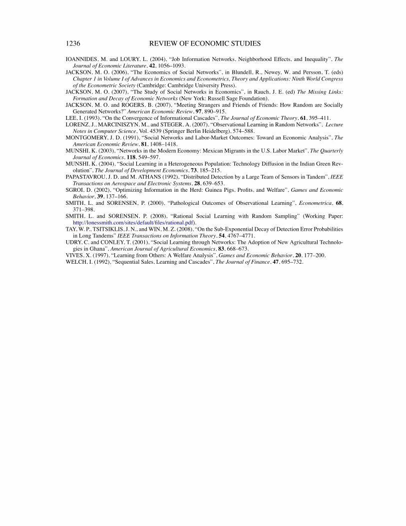
“rdr004” — 2011/10/17 — 7:35 — page 1236 — #36


IOANNIDES, M. and LOURY, L. (2004), “Job Information Networks, Neighborhood Effects, and Inequality”, TheJournal of Economic Literature, 42, 1056–1093.

JACKSON, M. O. (2006), “The Economics of Social Networks”, in Blundell, R., Newey, W. and Persson, T. (eds)Chapter 1 in Volume I of Advances in Economics and Econometrics, Theory and Applications: Ninth World Congressof the Econometric Society (Cambridge: Cambridge University Press).

JACKSON, M. O. (2007), “The Study of Social Networks in Economics”, in Rauch, J. E. (ed) The Missing Links:Formation and Decay of Economic Networks (New York: Russell Sage Foundation).

JACKSON, M. O. and ROGERS, B. (2007), “Meeting Strangers and Friends of Friends: How Random are SociallyGenerated Networks?” American Economic Review, 97, 890–915.

LEE, I. (1993), “On the Convergence of Informational Cascades”, The Journal of Economic Theory, 61, 395–411.LORENZ, J., MARCINISZYN, M., and STEGER, A. (2007), “Observational Learning in Random Networks”, Lecture

Notes in Computer Science, Vol. 4539 (Springer Berlin Heidelberg), 574–588.MONTGOMERY, J. D. (1991), “Social Networks and Labor-Market Outcomes: Toward an Economic Analysis”, The

American Economic Review, 81, 1408–1418.MUNSHI, K. (2003), “Networks in the Modern Economy: Mexican Migrants in the U.S. Labor Market”, The Quarterly

Journal of Economics, 118, 549–597.MUNSHI, K. (2004), “Social Learning in a Heterogeneous Population: Technology Diffusion in the Indian Green Rev-olution”, The Journal of Development Economics, 73, 185–215.

PAPASTAVROU, J. D. and M. ATHANS (1992), “Distributed Detection by a Large Team of Sensors in Tandem”, IEEETransactions on Aerospace and Electronic Systems, 28, 639–653.

SGROI, D. (2002), “Optimizing Information in the Herd: Guinea Pigs, Profits, and Welfare”, Games and EconomicBehavior, 39, 137–166.

SMITH, L. and SORENSEN, P. (2000), “Pathological Outcomes of Observational Learning”, Econometrica, 68,371–398.

SMITH, L. and SORENSEN, P. (2008), “Rational Social Learning with Random Sampling” (Working Paper:http://lonessmith.com/sites/default/files/rational.pdf).

TAY,W. P., TSITSIKLIS, J. N., andWIN, M. Z. (2008), “On the Sub-Exponential Decay of Detection Error Probabilitiesin Long Tandems” IEEE Transactions on Information Theory, 54, 4767–4771.

UDRY, C. and CONLEY, T. (2001), “Social Learning through Networks: The Adoption of New Agricultural Technolo-gies in Ghana”, American Journal of Agricultural Economics, 83, 668–673.

VIVES, X. (1997), “Learning from Others: A Welfare Analysis”, Games and Economic Behavior, 20, 177–200.WELCH, I. (1992), “Sequential Sales, Learning and Cascades”, The Journal of Finance, 47, 695–732.

Documents

Bayesian Learning in Social Networks - NYUpages.stern.nyu.edu/~ilobel/socialnetworks_revised.pdf · BAYESIAN LEARNING IN SOCIAL NETWORKS 1203 orseveralagentsrandomlydrawnfromtheentireortherecentpast.Ourrepresentationalsodoes