Embed Size (px)
Citation preview
MARKETING SCIENCEVol. 37, No. 2, March–April 2018, pp. 216–235
http://pubsonline.informs.org/journal/mksc/ ISSN 0732-2399 (print), ISSN 1526-548X (online)
Bayesian Nonparametric Customer Base Analysis withModel-Based VisualizationsRyan Dew,a Asim AnsariaaColumbia Business School, Columbia University, New York, New York 10027Contact: [email protected] (RD); [email protected] (AA)
Received: November 8, 2015Revised: July 19, 2016; November 21, 2016Accepted: December 12, 2016Published Online in Articles in Advance:January 17, 2018
https://doi.org/10.1287/mksc.2017.1050
Copyright: © 2018 INFORMS
Abstract. Marketing managers are responsible for understanding and predicting cus-tomer purchasing activity. This task is complicated by a lack of knowledge of all of thecalendar time events that influence purchase timing. Yet, isolating calendar time vari-ability from the natural ebb and flow of purchasing is important for accurately assess-ing the influence of calendar time shocks to the spending process, and for uncoveringthe customer-level purchasing patterns that robustly predict future spending. A com-prehensive understanding of purchasing dynamics therefore requires a model that flex-ibly integrates known and unknown calendar time determinants of purchasing withindividual-level predictors such as interpurchase time, customer lifetime, and numberof past purchases. In this paper, we develop a Bayesian nonparametric framework basedon Gaussian process priors, which integrates these two sets of predictors by modelingboth through latent functions that jointly determine purchase propensity. The estimatesof these latent functions yield a visual representation of purchasing dynamics, whichwe call the model-based dashboard, that provides a nuanced decomposition of spendingpatterns. We show the utility of this framework through an application to purchasing infree-to-play mobile video games. Moreover, we show that in forecasting future spending,our model outperforms existing benchmarks.
History: Peter Rossi served as the senior editor and Michel Wedel served as associate editor for thisarticle.
Supplemental Material: Data and the online appendix are available at https://doi.org/10.1287/mksc.2017.1050.
Keywords: customer base analysis • dynamics • analytics dashboards • Gaussian process priors • Bayesian nonparametrics • visualization •mobile commerce
1. IntroductionMarketers in multi-product companies face the daunt-ing task of understanding the ebb and flow of aggre-gate sales within and across many distinct customerbases. Such spending dynamics stem from the naturalstochastic process of purchasing characterized by cus-tomers’ interpurchase times, lifetimes with the firm,and number of past purchases, and from the influenceof managerial actions and shocks operating in calen-dar time. These other shocks are often outside the con-trol of the company, and include events such as holi-days, barriers to purchasing such as website outages,and competitor actions. While individual-level factorssuch as the recency of purchasing are often powerfulpredictors of future spending activity, managers thinkand act in calendar time. Hence, to successfully executea customer-centric marketing strategy, managers needto understand how calendar time events interact withindividual-level effects in generating aggregate sales.An accurate accounting of the underlying drivers of
spending is not possible unless individual-level andcalendar time effects are simultaneously modeled. Forexample, in spending models that omit calendar time
and rely solely on individual-level effects, momentarydisruptions in spending that occur in calendar timemaybe erroneously conflated with predictable, individual-level purchase propensities. Similarly, a small bump inspending on any given calendar day could representrandom noise if many customers are still active on thatday, or a significant calendar time event if only a fewcustomers are still active. Significantly, activity level isunobserved, but can be captured by individual-levelvariables such as interpurchase time. Flexibly includ-ing both types of effects in an individual-level purchasepropensity model is thus crucial for dynamic customerbase analysis, and the development of such a frame-work is our primary objective.
In this paper, we describe a flexible and robustBayesian nonparametric framework for customer baseanalysis that accomplishes that objective by proba-bilistically modeling purchase propensities in termsof underlying dynamic components. We demonstratethe utility of our new framework on spending datafrom mobile video games. Our model uses Gaussianprocess (GP) priors over latent functions to integrateevents that occur at multiple time scales and across
216

Dew and Ansari: Bayesian Nonparametric Customer Base AnalysisMarketing Science, 2018, vol. 37, no. 2, pp. 216–235, ©2018 INFORMS 217
different levels of aggregation, including calendar timeand individual-level time scales such as interpurchasetime, time since first purchase (customer lifetime), andnumber of past purchases. Its nonparametric specifica-tion allows for the flexible modeling of different pat-terns of effects, such that the model can be seamlesslyapplied across different customer bases and dynamiccontexts. The resulting latent function estimates facil-itate automatic model-based visualization and predic-tion of spending dynamics.Customer base analysis is central to modern market-
ing analytics. Contributions in this area have focusedon the stochastic modeling of individuals in termsof interpurchase time and lifetime, in contractualand noncontractual settings (Fader et al. 2005, 2010;Schmittlein et al. 1987; Schweidel and Knox 2013).These papers show that customer-level effects canexplain much of the variability of spending over time.However, they typically omit, or assume a prioriknown, calendar time effects. Events in calendar time,includingmarketing efforts and exogenous events suchas competitor actions, holidays, and day-of-the-weekeffects, can substantially impact spending in manyindustries. For digital products, such as those in ourapplication, relevant calendar events include productchanges simultaneously launched to all customers, andexogenous shocks such as website or e-commerce plat-form outages and crashes. Moreover, many of theseevents pose a common problem to marketing analysts:Although calendar time events undoubtedly influencespending rates, analysts may be unaware of the formof that influence or of the very existence of certainevents. This problem is exacerbated in larger compa-nies where the teams responsible for implementingmarketing campaigns or managing products may bedistinct from the analytics team, and where informa-tion may not flow easily across different organizationalsilos.
To cope with such information asymmetries andwith unpredictable spending dynamics, sophisticatedmanagers often rely on aggregate data methods, in-cluding exploratory data analyses, statistical processcontrol, time series models (Hanssens et al. 2001),and predictive data mining methods (Neslin et al.2006). These tools can forecast sales, model the impactof calendar time events, and provide metrics andvisual depictions of dynamic patterns that are easy tograsp. Unfortunately, these methods typically ignoreindividual-level predictors of spending, such as thosecaptured by customer base analysis models, whichprecludes their use in characterizing customer-levelspending behaviors and in performing tasks relevantto customer relationship management (CRM). Fur-thermore, not including these individual-level effectsmeans that these models cannot account for the latentactivity level of customers, which may, in turn, lead
to an inaccurate understanding of the true nature ofcalendar time events.
Building on the customer base analysis and aggre-gate data approaches, we use Bayesian nonparamet-ric GP priors to fuse together latent functions thatoperate over calendar time and over more traditionalindividual-level inputs, such as interpurchase time,customer lifetime, and purchase number. In this way,we integrate calendar time insights into the customerbase analysis framework. We use these latent func-tions in a discrete hazard specification to dynam-ically model customer purchase propensities, whilecontrolling for unobserved heterogeneity. We termthe resulting model the Gaussian Process PropensityModel (GPPM). While Bayesian nonparametrics havebeen successfully applied to marketing problems (e.g.,Ansari and Mela 2003, Wedel and Zhang 2004, Kimet al. 2007, Rossi 2014, Li and Ansari 2014), to ourknowledge, our paper is the first in marketing to takeadvantage of the powerful GPmethodology. Note that,although our paper applies GPs in the context of cus-tomer purchasing, GPs provide a general mechanismfor estimating latent functions, and can be used inmany other substantive contexts. We therefore alsoprovide an accessible introduction to GPs in general, toencourage their wider adoption in marketing.
In our application, the GP nonparametric frame-work means that the shapes of the latent propensityfunctions that govern purchasing are automaticallyinferred from the data, thus providing the flexibilityto robustly adapt to different settings, and to capturetime-varying effects, even when all of the informa-tion about inputs may not be available. The inferredlatent functions allow a visual representation of calen-dar time and individual-level patterns that character-ize spend dynamics, something that is not possible instandard probability models, where the output is oftena set of possibly unintuitive parameters. We refer to thecollection of these plots as themodel-based dashboard,as it gives a visual summary of the spending patternsin a particular customer base, and serves as a tool foranalyzing the spending dynamics in and across cus-tomer bases. Note that these model-based dashboardsare distinct from real-time dashboards that continu-ously stream various marketing metrics, such as thosedescribed in Pauwels et al. (2009).
In this paper, we begin by describing what GP priorsare (Section 2.1), and how they can be used to spec-ify latent dynamics in a model for dynamic customerbase analysis (Sections 2.2 and 2.3). We then apply ourmodel to spending data from two mobile video gamesowned by a large American video game publisher.These games are quite distinct, spanning different con-tent genres and target audiences. We show how theparameter estimates and accompanying model-baseddashboards generated from our approach can facilitate
Dew and Ansari: Bayesian Nonparametric Customer Base Analysis218 Marketing Science, 2018, vol. 37, no. 2, pp. 216–235, ©2018 INFORMS
managerial understanding of the key dynamics in eachcustomer base in the aggregate and at the individuallevel (Sections 3.1 and 3.2). We compare the GPPMto benchmark probability models, including differ-ent buy-till-you-die (BYTD) variants such as the beta-geometric/negative binomial distribution (BG/NBD)(Fader et al. 2005) and the Pareto-NBD (Schmittleinet al. 1987), hazard models with and without time-varying covariates (e.g., Gupta 1991, Seetharaman andChintagunta 2003), and variants of the discrete hazardapproach, including a sophisticated state-space speci-fication, and show that the GPPM significantly outper-forms these existing benchmarks in fit and forecastingtasks (Section 3.3). We conclude by summarizing thebenefits of our framework, citing its limitations, andidentifying areas of future research.
2. Modeling FrameworkIn our framework for dynamic customer base analy-sis, we focus on flexibly modeling individual-level pur-chase propensity. We model this latent propensity interms of the natural variability in purchase incidencedata along four dimensions, i.e., calendar time, inter-purchase time (recency), customer lifetime, and num-ber of past purchases. Our focus onmodeling purchaseincidence is consistent with the majority of the litera-ture on customer base analysis, and also fits nicely withour application area, wherewe focus on the purchasingof a single product, and where there is minimal vari-ability in spending amount.1 We use a discrete-timehazard framework to specify the purchase propensity,as most customer-level data are available at a discretelevel of aggregation. This is also the case in our appli-cation, where daily data are available.The observations in our data consist of a binary
indicator yi j that specifies whether customer i made apurchase at observation j, and a corresponding tuple(ti j , ri j , li j , qi j) containing the calendar time, recency,customer lifetime, and number of past purchases, re-spectively. Recency refers to interpurchase time, or thetime since the customer’s previous purchase, whilecustomer lifetime refers to the time since the customer’sfirst purchase. Depending on the context, a vector zi ofdemographics or other time invariant variables, suchas the customer acquisition channel or acquisition date,may also be available. The probability of customer ipurchasing is modeled as
Pr(yi j � 1)� logit−1[α(ti j , ri j , li j , qi j)+ z′iγ+ δi], (1)
where, logit−1(x) � 1/(1 + exp(−x)). We see in Equa-tion (1) that the purchasing rate is driven by a time-varying component α( · ) and two time invariant effects,z′iγ and δi , which capture the observed and unob-served sources of heterogeneity in base spending rates,respectively. This setupmodels spending dynamics via
aggregate trajectories, i.e., all customers are assumedto follow the same dynamic pattern, while maintain-ing individual heterogeneity in the spending processvia the random effect δi and using other observedindividual-specific variables, zi , when available. In ourapplication, we will focus exclusively on unobservedheterogeneity. Note that while calendar time is anaggregate time scale, the recency, lifetime, and pur-chase number dimensions are individual-level timescales. That is, customers may, at any given point in cal-endar time t, be at different positions in the (ri j , li j , qi j)subspace; therefore, the aggregate sales at any givencalendar time t are the amalgam of the activities of cus-tomers who differ widely in their expected purchasebehaviors.
The heart of our framework involves specificationof the purchase propensity, α(ti j , ri j , li j , qi j). We treatα( · ) as a latent function and model it nonparametri-cally using GP priors (Rasmussen and Williams 2006,Roberts et al. 2013). The nonparametric approach flex-ibly models random functions and allows us to auto-matically accommodate different patterns of spendingdynamics that may underlie a given customer base.These dynamics operate along all four of our dimen-sions. Furthermore, these dynamics may operate atdifferent time scales in a single dimension, includingsmooth long-run trends and short-term patterns, aswell as cyclic variations, which are inferred from thedata. To allow such rich structure, we use an additivecombination of unidimensional GPs to specify and esti-mate the multivariate function α(ti j , ri j , li j , qi j).
2.1. Gaussian Process PriorsWe begin by describing GPs and highlight how theycan nonparametrically capture rich, dynamic patternsin a Bayesian probability model. A GP is a stochas-tic process { f (τ): τ ∈ T } indexed by input elementsτ such that, for any finite set of input values, τ �{τ1 , τ2 , . . . , τM}, the corresponding set of function out-puts, f (τ) � { f (τ1), f (τ2), . . . , f (τM)}, follows a mul-tivariate Gaussian distribution. The characteristics ofthe stochastic process are defined by a mean func-tion and a covariance function, also called a kernel.For a fixed set of inputs, a GP reduces to the famil-iar multivariate Gaussian distribution, with a meanvector determined by the GP’s mean function, and acovariance matrix determined by its kernel. However,unlike a standardmultivariate normal distribution thatis defined over vectors of fixed length, a GP defines adistribution over outputs for any possible set of inputs.From a Bayesian perspective, this provides a naturalmechanism for probabilistically specifying uncertaintyover functions. Because the estimated function valuesare the parameters of a GP, the number of parametersgrows with the number of unique inputs, making themodel nonparametric.
Dew and Ansari: Bayesian Nonparametric Customer Base AnalysisMarketing Science, 2018, vol. 37, no. 2, pp. 216–235, ©2018 INFORMS 219
While GPs are often defined over multidimensionalinputs, for simplicity of exposition, we begin by assum-ing a unidimensional input, τ ∈ � (e.g., time). To fixnotation, suppose f is a function that depends on thatinput. Let τ be a vector of M input points, and let f (τ)be the corresponding vector of output function values.As described above, a GP prior over f is completelyspecified by amean function, m(τ)�E[ f (τ)], and a ker-nel, k(τ, τ′) � Cov[ f (τ), f (τ′)], that defines a positivesemidefinite covariance matrix
K(τ,τ)�©«
k(τ1 , τ1) k(τ1 , τ2) . . . k(τ1 , τM)k(τ2 , τ1) k(τ2 , τ2) . . . k(τ2 , τM)
......
. . ....
k(τM , τ1) k(τM , τ2) . . . k(τM , τM)
ª®®®®¬, (2)
over all of the outputs. We discuss specific forms of themean function and kernel in Sections 2.1.1 and 2.1.2.Generally, these functions are governed by a smallset of hyperparameters that embody certain traits ofthe GP. For instance, the squared exponential (SE)kernel, which we discuss in detail in Section 2.1.2,is given by kSE(τi , τ j) � η2 exp{−(τi − τ j)2/(2ρ2)}. Thisform encodes the idea that nearby inputs should haverelated outputs through two hyperparameters, i.e., anamplitude, η, and a smoothness, ρ. Intuitively, thesetwo hyperparameters determine the traits of the func-tion space being modeled by a GP with this kernel.Given a fixed vector of inputs τ, letting f (τ) ∼
GP (m(τ), k(τ, τ′)) is equivalent to modeling the vec-tor of function outputs via a marginal multivari-ate Gaussian f (τ) ∼ N (m(τ),K(τ, τ)). The mean m(τ)and covariance matrix K(τ, τ) of the above multivari-ate normal marginal distribution are parsimoniouslydetermined through the small set of hyperparametersunderlying the mean function and kernel of the GP.The fact that the marginal of a GP is a multivariatenormal distribution makes it easy to comprehend howfunction interpolation and extrapolation work in thisframework. Conditioned on an estimate for the func-tion values at the observed inputs, and on the meanfunction and kernel hyperparameters, the output val-ues for the latent function f for some new input pointsτ∗ can be predicted using the conditional distributionof a multivariate normal. Specifically, the joint distri-bution of the old and new function values is given by[
f (τ)f (τ∗)
]∼N
( [m(τ)m(τ∗)
],
[K(τ, τ) K(τ, τ∗)K(τ∗ , τ) K(τ∗ , τ∗)
] ). (3)
Hence, the conditional distribution of the new outputscan be written as
f (τ∗) ∼N (m(τ∗)+K(τ∗ , τ)K(τ, τ)−1[ f (τ) −m(τ)],K(τ∗ , τ∗) −K(τ∗ , τ)K(τ, τ)−1K(τ, τ∗)). (4)
This equation makes clear that the kernel and meanfunctions determine the distribution of the output val-ues for existing and new inputs. As the mean andcovariance of the marginal multivariate normal areparametrized via the mean and kernel functions, theGP remains parsimonious, and can seamlessly inter-polate and extrapolate for any set of input values. Thechoice of mean function allows us to model differenta priori expected functional forms, while the kerneldetermines how much the functions deviate nonpara-metrically from that mean function.2.1.1. Mean Functions. The mean function capturesexpected functional behaviors. Within the range ofobserved inputs, the mean function often has littleinfluence over the estimated function values; instead,the properties of the estimated function are largelydetermined by the kernel, as we describe in Sec-tion 2.1.2. Because of this, in many GP applications, themean function is set to a constant, reflecting no priorassumptions about functional form. However, far fromthe range of observed inputs, the posterior expectedfunction values revert to the mean function.2 In someapplications, this mean reverting behavior combinedwith a constant mean function is problematic, as wemay expect the function values to be increasing ordecreasing, in and out of the range of inputs. To cap-ture this expected behavior, we may choose to use anonconstant mean function.In this paper, we use a constant mean function or
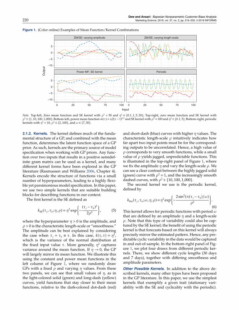
a parametric monotonic power mean function, givenby m(τ) � λ1(τ − 1)λ2 , λ2 > 0. This specification cap-tures expected monotonic behavior, while allowing fora decreasing marginal effect over the input.3 We useτ− 1 and restrict λ2 > 0, to be consistent with our iden-tification restrictions that we describe in Section 2.2.4.We emphasize that the mean function sets an expec-tation over function values, but does not significantlyrestrict them. TheGP structure allows functions to non-parametrically deviate from the mean function, result-ing in function estimates that differ from the mean’sparametric form. This is obvious in all panels of Fig-ure 1, where we plot random draws from GPs with dif-ferent mean functions and kernels. Across the panelsof Figure 1, we see shapes that are sometimes dramati-cally different from the respective constant and powermean functions that generated them. The main role ofthemean function is in extrapolating far from the rangeof the observed inputs, where it determines expectedfunction behavior in the absence of data. While weuse only these two mean functions as a simple way ofcapturing our prior expectations, any parametric formcould be used as a mean function. Given the capac-ity of the GP to capture deviations from parametricforms, it is generally considered best practice to usesimple mean functions, and let the GP capture anycomplexities.
Dew and Ansari: Bayesian Nonparametric Customer Base Analysis220 Marketing Science, 2018, vol. 37, no. 2, pp. 216–235, ©2018 INFORMS
Figure 1. (Color online) Examples of Mean Function/Kernel Combinations
ZM/SE; varying amplitude ZM/SE; varying length-scale
Power MF; SE kernel Periodic
−10
−5
0
5
−10
−5
0
5
0 25 50 75 100 0 25 50 75 100
Input
Out
put
Note. Top-left, Zero mean function and SE kernel with ρ2 � 50 and η2 ∈ {0.1, 1, 5, 20}; Top-right, zero mean function and SE kernel withρ2 ∈ {1, 10, 100, 1,000}; Bottom-left, powermean function m(τ)�±2(τ−1)0.3 and SE kernel with ρ2 � 100 and η2 ∈ {0.1, 5}; Bottom-right, periodickernels with η2 � 10, ρ2 ∈ {2, 100}, and ω ∈ {7, 30}.
2.1.2. Kernels. The kernel defines much of the funda-mental structure of a GP, and combined with the meanfunction, determines the latent function space of a GPprior. As such, kernels are the primary source of modelspecification when working with GP priors. Any func-tion over two inputs that results in a positive semidef-inite gram matrix can be used as a kernel, and manydifferent kernel forms have been explored in the GPliterature (Rasmussen and Williams 2006, Chapter 4).Kernels encode the structure of functions via a smallnumber of hyperparameters, leading to a highly flexi-ble yet parsimoniousmodel specification. In this paper,we use two simple kernels that are suitable buildingblocks for describing functions in our context.The first kernel is the SE defined as
kSE(τ j , τk ; η, ρ)� η2 exp{−(τ j − τk)2
2ρ2
}, (5)
where the hyperparameter η > 0 is the amplitude, andρ > 0 is the characteristic length-scale or “smoothness.”The amplitude can be best explained by consideringthe case when τ j � τk ≡ τ. In this case, k(τ, τ) � η2,which is the variance of the normal distribution atthe fixed input value τ. More generally, η2 capturesvariance around the mean function. If η→ 0, the GPwill largely mirror its mean function. We illustrate thisusing the constant and power mean functions in theleft column of Figure 1, where we randomly drawGPs with a fixed ρ and varying η values. From thesetwo panels, we can see that small values of η, as inthe light-colored solid (green) and long-dash (yellow)curves, yield functions that stay closer to their meanfunctions, relative to the dark-colored dot-dash (red)
and short-dash (blue) curves with higher η values. Thecharacteristic length-scale ρ intuitively indicates howfar apart two input points must be for the correspond-ing outputs to be uncorrelated. Hence, a high value ofρ corresponds to very smooth functions, while a smallvalue of ρ yields jagged, unpredictable functions. Thisis illustrated in the top-right panel of Figure 1, wherewe fix the amplitude η and vary the length-scale ρ. Wecan see a clear contrast between the highly jagged solid(green) curve with ρ2 � 1, and the increasingly smoothdashed curves, with ρ2 ∈ {10, 100, 1,000}.
The second kernel we use is the periodic kernel,defined by
kPer(τ j , τk ;ω, η, ρ)� η2 exp{−
2sin2(π(τ j − τk)/ω)ρ2
}.
(6)This kernel allows for periodic functions with period ωthat are defined by an amplitude η and a length-scaleρ. Note that this type of variability could also be cap-tured by the SE kernel; the benefit of using the periodickernel is that forecasts based on this kernel will alwaysprecisely mirror the estimated pattern. Hence, any pre-dictable cyclic variability in the datawould be capturedin and out-of-sample. In the bottom-right panel of Fig-ure 1, we plot four draws from different periodic ker-nels. There, we show different cycle lengths (30 daysand 7 days), together with differing smoothness andamplitude parameters.Other Possible Kernels. In addition to the above de-scribed kernels, many other types have been proposedin the GP literature. In this paper, we use the simplestkernels that exemplify a given trait (stationary vari-ability with the SE and cyclicality with the periodic).

Dew and Ansari: Bayesian Nonparametric Customer Base AnalysisMarketing Science, 2018, vol. 37, no. 2, pp. 216–235, ©2018 INFORMS 221
These are by far the most commonly used kernels, theSE especially serving as the workhorse kernel for thebulk of the GP literature. Additional kernels includethe rational quadratic, which can be derived as an infi-nitemixture of SE kernels, and the large class ofMaternkernels, which can capture different levels of differen-tiability in function draws.2.1.3. Additivity. Just as the sum of Gaussian variatesis distributed Gaussian, the sum of GPs is also a GP,with a mean function equal to the sum of the meanfunctions of the component GPs, and its kernel is equalto the sum of the constituent kernels. This is called theadditivity property of GPs, which allows us to definea rich structure even along a single dimensional input.Specifically, the additivity property allows us to modelthe latent function f as a sum of subfunctions on thesame input space, f (τ)� f1(τ)+ f2(τ)+ · · ·+ f J(τ), whereeach of these subfunctions can have its ownmean func-tion, m j(τ), and kernel, k j(τ, τ′). The mean functionand kernel of the function f are then given by m(τ) �∑J
j�1 m j(τ) and k(τ, τ′)�∑Jj�1 k j(τ, τ′), respectively. This
allows us to flexibly represent complex patterns ofdynamics even when using simple kernels such as theSE.We can, for example, allow the subfunctions to havedifferent SE kernels that capture variability along dif-ferent length-scales, or add a periodic kernel to isolatepredictable cyclic variability of a given cycle length. Itis through this additive mechanism that we representlong-run and short-run variability in a given dimen-sion, for instance, or isolate predictable periodic effectsfrom unpredictable noise, as discussed in Section 2.2.4Up to now, we have focused on illustrating GPs in uni-dimensional contexts. We now show how additivitycan be leveraged to construct GPs formultidimensionalfunctions.2.1.4. Multidimensional GPs. In practice, we are ofteninterested in estimating a multidimensional function,such as the α( · ) function in Equation (1). Let h( · ) be ageneric multidimensional function from �D to �. Theinputs to such a function are vectors of the form τm ≡(τ(1)m , τ
(2)m , . . . , τ
(D)m ) ∈ �D , for m � 1, . . . ,M, such that the
set of all inputs is an M ×D matrix. Just as in the uni-dimensional case, h( · ) can also be modeled via a GPprior. While there are many ways in which multi-inputfunctions can be modeled via GPs, a simple yet power-ful approach is to consider h( · ) as a sum of single inputfunctions, h1( · ), h2( · ), . . . , hD( · ), and to model each ofthese unidimensional functions as a unidimensionalGP with its own mean function and kernel structure(Duvenaud et al. 2013). The additivity property impliesthat additively combining a set of unidimensional GPsover each dimension of the function is equivalent tousing a particular sum kernel GP on the whole, mul-tidimensional function. We use such an additive struc-ture to model α(ti j , ri j , li j , qi j) in the GPPM.
Additively separable GPs offer many benefits: First,they allow us to easily understand patterns alonga given dimension, and they facilitate visualization,as the subfunctions are unidimensional. Second, theadditivity property implies that the combined stochas-tic process is also a GP. Finally, the separable struc-ture reduces computational complexity. Estimating aGP involves inverting its kernel matrix. This inversionrequires O(M3) computational time and O(M2) stor-age demands for M inputs. In our case, as the inputs(ti j , ri j , li j , qi j) can only exist on a grid of fixed values,we will have L < M inputs, where L corresponds to allunique observed (ti j , ri j , li j , qi j) combinations. Despitethe reduction, this is a very large number of inputs,and would result in considerable computational com-plexity without the separable structure. The additivespecification reduces this computational burden to thatof inverting multiple (in our case, six) T × T matrices,where T �M is the number of time periods observedin the data.
2.1.5. GPs vs. Other Function EstimationMethods. AsGP priors are new to marketing, it is worthwhile tobriefly summarize the rationale for using them, insteadof other flexible methods for modeling latent functionssuch as simple fixed effects, splines or state space mod-els. Foremost, GPs facilitate a structured decomposi-tion of a single process into several subprocesses viathe additivity property. This additive formulation facil-itates a rich representation of a dynamic process viaa series of kernels that capture patterns of differentforms (e.g., periodic versus nonperiodic) and operateat different time scales. Yet, as the sum of GPs is a GP,the specification remains identified, with a particularmean and covariance kernel. Achieving a similar rep-resentation with other methods is infeasible or moredifficult.5 Moreover, GPs are relatively parsimonious,and when estimated in a Bayesian framework, tend toavoid overfitting. Bayesian estimation of GPs involvesjointly estimating the function values and hyperparam-eters, thus determining the traits of the function andthe function values themselves. As the flexibility of thelatent functions is controlled via a small number ofhyperparameters, we retain parsimony. Moreover, thestructure of the marginal likelihood of GPs, obtainedby integrating out the function values, clearly showshow the model makes an implicit fit versus complex-ity trade-off whereby function flexibility, as capturedby the hyperparameters, is balanced by a penalty thatresults in the regularization of the fit (for details, seeRasmussen and Williams 2006, Section 5.4.1).
2.2. Full Model SpecificationThe flexibility afforded by GP priors makes them es-pecially appropriate for modeling our latent, time-
Dew and Ansari: Bayesian Nonparametric Customer Base Analysis222 Marketing Science, 2018, vol. 37, no. 2, pp. 216–235, ©2018 INFORMS
varying function, α(ti j , ri j , li j , qi j). Recall that the basicform of the GPPM is
Pr(yi j � 1)� logit−1[α(ti j , ri j , li j , qi j)+ z′iγ+ δi]. (7)
For ease of exposition, we subsequently omit the i jsubscripts. For simplicity and to reduce computationalcomplexity, we assume an additive structure
α(t , r, l , q)� αT(t)+ αR(r)+ αL(l)+ αQ(q), (8)
and model each of these functions using separate GPpriors. This structure and the nonlinear nature of themodel implies an interaction between the effects: Forexample, if the recency effect is very negative, calendartime events can do little to alter the spend probabil-ity. While additivity is a simplifying assumption, inour application, this compensatory structure seems toexplain the data well.To specify each of these additive components, we
return to the mean functions and kernels outlined inSections 2.1.1 and 2.1.2, and to the additivity propertyof GPs from Section 2.1.3. Recall that themean functionencodes the expected functional behavior: With theconstant mean function, we impose no expectations;with the power mean function, we encode expectedmonotonicity. The kernel choice endows the GP withadditional properties: A single SE kernel allows flexi-ble variation with one characteristic length-scale, whilethe periodic kernel allows the GP to exhibit predictablecyclic behavior of a given periodicity. Additivity allowsus to combine these kernel properties, to achieve vari-ation along more than one length-scale or to isolatepredictable cyclic behavior in a given dimension. Wecan use these general traits of mean function and ker-nel combinations to specify our model based on theexpected nature of the variation along a given dimen-sion. Below, we explain the specification used in ourapplication. The GPPM framework is highly flexible:Throughout the following sections, we also explainhow this specification can be modified to handle moregeneral settings.
2.2.1. Calendar Time. In calendar time, we expect twoeffects to operate, i.e., long-run trends and short-rundisturbances. These short run events could includepromotions, holidays or other shocks to the purchas-ing process. Furthermore, we expect cyclicality suchthat purchasing could be higher on weekends than onweekdays, or in particular months or seasons. As wedescribe in Section 3, in our application, given the spanof our data, we expect only one periodic day of theweek (DoW) effect. Together, this description of spend-ing dynamics implies a decomposition of αT into threesubcomponents
αT(t)� αLongT (t)+ αShort
T (t)+ αDoWT (t), (9)
where we model each component such that,
αLongT (t) ∼ GP (µ, kSE(t , t′; ηTL , ρTL)),αShortT (t) ∼ GP (0, kSE(t , t′; ηTS , ρTS)),αDoWT (t) ∼ GP (0, kPer(t , t′;ω � 7, ηTW , ρTW)).
Without loss of generality, we impose ρTL > ρTS,to ensure that the long-run component captures asmoother variation than the short-run component. Weuse constant mean functions here because, a priori, wedo not wish to impose any assumptions about calen-dar time behavior. The constant mean µ in the long-run component captures the base spending rate in themodel. Far from the range of the data, this specifica-tion implies that the posterior mean of these effects willrevert to this base spending rate, reflecting our lack ofa priori knowledge about these effects.
This specification is very general, and has showngood performance in our application, where we illus-trate the kinds of trends and disturbances that can becaptured across these two components.6 Furthermore,the modularity of the additive GP specification allowseasy modifications to accommodate different settings.Longer spans of data may contain variability in spend-ing along different length-scales, which may requireadditional SE components. There may also be sev-eral periodicities requiring additional periodic compo-nents. These can be easily included additively.2.2.2. Individual-Level Effects. The remaining effects,i.e., recency, lifetime, and purchase number, operateat the customer level. In most applications, we donot expect short-run shocks along these inputs. Wedo, however, expect monotonicity. For instance, intu-itively, we expect spending probability to be generallydecreasing in interpurchase time. Similarly, we expectspending probability to be generally increasing in pur-chase number,7 and to be generally decreasing in cus-tomer lifetime. Furthermore, while we expect mono-tonicity, we also expect a decreasing marginal effect.For example, we expect a priori that the differencebetween having spent 5 versus 10 days ago is quite dif-ferent than the difference between having spent 95 ver-sus 100 days ago. Together, these expected traits justifyusing our power mean function
αR(r) ∼ GP (λR1(r − 1)λR2 , kSE(r, r′; ηR , ρR)),αL(l) ∼ GP (λL1(r − 1)λL2 , kSE(l , l′; ηL , ρL)),αQ(q) ∼ GP (λQ1(r − 1)λQ2 , kSE(r, r′; ηQ , ρQ)).
This specificationallows for long-runmonotonic behav-ior, even out-of-sample, as captured by the meanfunction, and for nonparametric deviations from thisexpected functional form, as captured by the SE ker-nel. We believe that this specification is very generaland widely applicable. In some cases, however, more

Dew and Ansari: Bayesian Nonparametric Customer Base AnalysisMarketing Science, 2018, vol. 37, no. 2, pp. 216–235, ©2018 INFORMS 223
nuance may be required in specifying these effects toaccommodate companyactions that occur on these timescales. If, for instance, the company offers promotionsbased on loyalty, these effectswill operate along the life-time dimension. In that case, the lifetime componentcan be modeled similar to the calendar time compo-nent, with an additive SE component to capture theseshort-run deviations from the long-run, decreasingtrend embodied in the above specification. See OnlineAppendix B for an example of this modification.
2.2.3. Heterogeneity, Random Effects, and Priors. Weaccommodate unobserved heterogeneity by assumingthat the random effect δi comes from a normal pop-ulation distribution, i.e., δi ∼ N (0, σ2). In our applica-tion, we found no significant time-invariant effects zi ;hence, we omit z′iγ from our model going forward.We estimate the model in a fully Bayesian fashion, andtherefore specify priors over all unknowns, includingthe GP hyperparameters. We use the fact that mean-ingful variation in the inverse logit function occursfor inputs between −6 and 6; hence, meaningful dif-ferences in the inputs to the GPPM will also occurbetween −6 and 6 to select proper weakly informativeNormal and Half-Normal prior distributions that giveweight to variations in this range. Specifically, we letthe population variance σ2 ∼ Half-Normal(0, 2.5) andthe base spending rate µ ∼N (0, 5). For the SE hyperpa-rameters, we specify η2 ∼ Half-Normal(0, 5) and ρ2 ∼Half-Normal(T/2,T). For the mean function, we letλ1 ∼ N (0, 5), and let λ2 ∼ Half-Normal(0, 5). Signifi-cantly, the fully Bayesian approach, whereby the GPfunction values and their associated hyperparametersare estimated from the data, allows us to automati-cally infer the nature of the latent functions that drivespending propensity.
2.2.4. Identification. We need to impose identificationrestrictions because of the additive structure of ourmodel. Sums of two latent functions, such as α1(t) +α2(t), are indistinguishable from α∗1(t) + α∗2(t), whereα∗1(t) � α1(t) + c, and α∗2(t) � α2(t) − c for some c ∈ �,as both sums imply the same purchase probabilities.To address this indeterminacy, we set the initial func-tion value (corresponding to input τ � 1) to zero forall of the latent functions, except for αLong
T (t). In thissense, αLong
T (t), with its constant mean function µ, cap-tures the base spending rate for new customers, andthe other components capture deviations from that, astime progresses. Whenever we implement a sum of SEkernels, as in the calendar time component, we alsoconstrain the length-scale parameters to be ordered toprevent label switching. All of these constraints are eas-ily incorporated in our estimation algorithm, describedbelow.
2.3. EstimationWe use a fully Bayesian approach for inference. Forconcision, let αi j ≡ α(ti j , ri j , li j , qi j), which in our spec-ification, is equivalent to αi j � α
LongT (ti j) + αShort
T (ti j) +αDoWT (ti j)+ αR(ri j)+ αL(li j)+ αQ(qi j). To further simplify
notation, we let the independent components of thesum be indexed by k, with generic inputs τk , such thatthis GP sum can bewritten as αi j �
∑Kk�1 αk(τki j
). Each ofthese components is governed by a set of hyperparame-ters, as outlined in Section 2.2, denoted here asφk , withthe collection of all hyperparameters denoted as φ.Finally, for each component, we let the vector of func-tion values over all possible inputs along that dimen-sion be denoted asαk .With this simplified notation, thejoint density of the data and the model unknowns is
p(y, {αk},δ,φ, σ2)�[ I∏
i�1
Mi∏j�1
p(yi j | αi j , δi)p(δi | σ2)]
·[ K∏
k�1p(αk | φk)
]p(σ2)p(φ). (10)
As the full posterior distribution p({αk},δ,φ, σ2 | y)is not available analytically, we use Markov ChainMonte Carlo (MCMC) methods to draw samples ofthe unknown function values, random effects, popu-lation parameters, and GP hyperparameters from theposterior.
As the function values and the hyperparameters donot have closed-form full conditionals, our setup isnonconjugate, and Gibbs sampling is not an option.Moreover, as the function values and the hyperparam-eters typically exhibit strong posterior dependence,ordinaryMetropolis–Hastings procedures that explorethe posterior via a random walk are not efficient. Wetherefore use the Hamiltonian Monte Carlo (HMC)algorithm that leverages the gradient of the posteriorto direct the exploration of the Markov chain to avoidrandom-walk behavior. HMC methods are ideal fornonconjugate GP settings such as ours, as they canefficiently sample the latent function values as well asthe hyperparameters (Neal 1998). In particular, we usethe No U-Turn Sampling (NUTS) variant of HMC asimplemented in the Stan probabilistic programminglanguage (Hoffman and Gelman 2014, Carpenter et al.2017). SeeOnlineAppendixA for an overview ofHMC.
Stan has recently gained traction as an efficientand easy-to-use probabilistic programming tool forBayesian modeling. We use Stan as it is an efficientimplementation of adaptive HMC. Stan programs aresimple to write and modify, and therefore facilitateeasy experimentation, without the need for extensivereprogramming. This is important for the wider adop-tion of this framework in practice.8 Finally, given theefficiency of HMC and Stan, convergence, as measuredby the R̂ statistic (Gelman and Rubin 1992), is achieved
Dew and Ansari: Bayesian Nonparametric Customer Base Analysis224 Marketing Science, 2018, vol. 37, no. 2, pp. 216–235, ©2018 INFORMS
in as few as 400 iterations, although in this paper allestimation is done with 4,000 iterations; the first 2,000are used for burn-in.
3. ApplicationWe apply our framework to understand the spendingdynamics in two free-to-play mobile games from oneof the world’s largest video game companies. The datatake the form of simple spend incidence logs, with userIDs and time stamps.9 In free-to-play (or “freemium”)settings, users can install and play video games ontheir mobile devices for free, and are offered oppor-tunities to purchase within the game. These spend-ing opportunities typically involve purchasing in-gamecurrency, such as coins, that may subsequently be usedto progress more quickly through a game, obtain rareor limited edition items to use with their in-game char-acters or to otherwise gain a competitive edge overnonpaying players. Clearly, the nature of these pur-chases will depend on the game, which is why it isimportant for a model of spending behavior to be fullyflexible in its specification of the regular, underlyingdrivers of purchasing. We cannot name the games herebecause of nondisclosure agreements. Instead, we usethe general descriptors Life Simulator (LS) and CityBuilder (CB) to describe the games.The games and ranges of data used were selected by
our data provider to understand spending dynamicsover specific periods of time. We use a random sam-ple of 10,000 users for each of the two games. Eachsample is drawn from users who installed the gamein the first 30 days, and spent at least once during thetraining window. We used 8,000 users for estimation,and 2,000 for cross-validation. In the LS game, play-ers create an avatar, and then live a digital life as thatavatar. Purchases in this context can be rare or lim-ited edition items to decorate or improve their avataror its surroundings. Oftentimes, limited edition itemsare themed according to holidays such as Christmas or
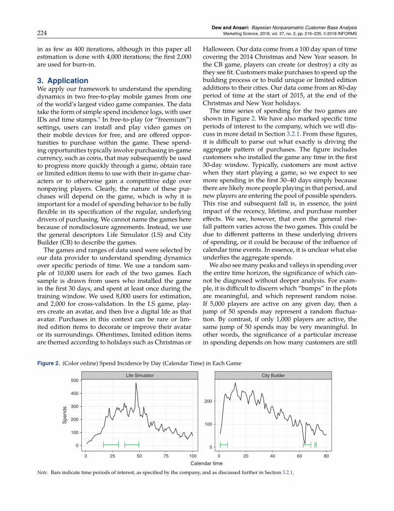
Figure 2. (Color online) Spend Incidence by Day (Calendar Time) in Each Game
Life Simulator City Builder
0
100
200
300
400
500
0
100
200
0 25 50 75 100 0 20 40 60 80
Calendar time
Spe
nds
Note. Bars indicate time periods of interest, as specified by the company, and as discussed further in Section 3.2.1.
Halloween. Our data come from a 100 day span of timecovering the 2014 Christmas and New Year season. Inthe CB game, players can create (or destroy) a city asthey see fit. Customers make purchases to speed up thebuilding process or to build unique or limited editionadditions to their cities. Our data come from an 80-dayperiod of time at the start of 2015, at the end of theChristmas and New Year holidays.
The time series of spending for the two games areshown in Figure 2. We have also marked specific timeperiods of interest to the company, which we will dis-cuss in more detail in Section 3.2.1. From these figures,it is difficult to parse out what exactly is driving theaggregate pattern of purchases. The figure includescustomers who installed the game any time in the first30-day window. Typically, customers are most activewhen they start playing a game, so we expect to seemore spending in the first 30–40 days simply becausethere are likelymore people playing in that period, andnew players are entering the pool of possible spenders.This rise and subsequent fall is, in essence, the jointimpact of the recency, lifetime, and purchase numbereffects. We see, however, that even the general rise-fall pattern varies across the two games. This could bedue to different patterns in these underlying driversof spending, or it could be because of the influence ofcalendar time events. In essence, it is unclear what elseunderlies the aggregate spends.
We also seemany peaks and valleys in spending overthe entire time horizon, the significance of which can-not be diagnosed without deeper analysis. For exam-ple, it is difficult to discern which “bumps” in the plotsare meaningful, and which represent random noise.If 5,000 players are active on any given day, then ajump of 50 spends may represent a random fluctua-tion. By contrast, if only 1,000 players are active, thesame jump of 50 spends may be very meaningful. Inother words, the significance of a particular increasein spending depends on how many customers are still

Dew and Ansari: Bayesian Nonparametric Customer Base AnalysisMarketing Science, 2018, vol. 37, no. 2, pp. 216–235, ©2018 INFORMS 225
actively spending at that time, which in turn dependson the individual-level recency, lifetime, and purchasenumber effects. An accurate accounting of the impactof calendar-time events cannot be made without con-sidering these individual-level predictors of spending.Thus, it is important to develop a model-based under-standing of the underlying spend dynamics, which iswhat we do via the GPPM.
3.1. Model Output and FitTheGPPMoffers a visual and highly general system forcustomer base analysis driven by nonparametric latentspending propensity functions. These latent curves arethe primary parameters of the model, and their poste-rior estimates are shown in Figure 3 for LS, and Figure 4for CB. We call these figures the GPPM dashboards,as they visually represent latent spending dynamics.As we will see in Section 3.2, these dashboards can beused toaccomplishmanyof thegoalswehavediscussedthroughout theprevious sections, including forecastingspending, understanding purchasing at the individual-level, assessing the influence of calendar time events,and comparing spending patterns across products.These dashboards are underpinned by a set of hy-
perparameters, and estimated jointly with a randomeffects distribution capturing unobserved heterogene-ity. Posterior medians of these parameters are shownin Table 1. While the hyperparameters summarize the
Figure 3. (Color online) Posterior Dashboard for the Life Simulator Customer Base
Calendar, long-run Calendar, short-run Calendar, weekly
Recency Lifetime Purchase number
−1.8
−1.6
−1.4
−1.2
0
0.5
−0.3
−0.2
−0.1
0
0.1
−8
−6
−4
−2
0
−1.0
−0.5
0
0
0.25
0.50
0.75
1.00
0 25 50 75 100 0 25 50 75 100 0 25 50 75 100
0 25 50 75 100 0 25 50 75 100 0 20 40
Input
Fun
ctio
n va
lue
Notes. The curves are the median posterior estimates for the latent components of α(t , r, l , q) with 95% credible intervals. The blue plots (toprow) are the calendar time components, while the red plots (bottom row) are the individual-level effects. The marked time periods (green bars)are areas of interest to the company, as discussed in Section 3.2.1.
traits of the estimated dashboard curves, as explainedin Section 2.1, we can gain a greater understanding ofthe dynamics from an analysis of the estimated dash-board curves themselves, as we do in subsequent sec-tions. The other parameters in Table 1 are the basespending rate, µ, and the population variance of therandom effects distribution, σ2, which reflects the levelof heterogeneity in base spending rates estimated ineach customer base.3.1.1. Model Fit. First, to validate our model, we lookat its fit to the observed daily spending data in thecalibration sample of 8,000 customers and in the hold-out sample of 2,000 customers. Because a closed-formexpression is not available for the expected numberof aggregate counts in the GPPM, we simulate spend-ing from the posterior predictive distribution usingthe post-convergence HMC draws for each parameter,including the latent curves and random effects. Thetop row of Figure 5 shows the actual spending andthe median simulated purchase counts (dashed line)for the two games, along with 95% posterior predictiveintervals.
We see that the fit is exceptional, and almost per-fectly tracks the actual purchases in both cases. Thisis not surprising, as we model short-run deviationsin the probability of spending on a daily basis andtherefore essentially capture the residuals from thesmoother model components. That is, the short-run

Dew and Ansari: Bayesian Nonparametric Customer Base Analysis226 Marketing Science, 2018, vol. 37, no. 2, pp. 216–235, ©2018 INFORMS
Figure 4. (Color online) Posterior Dashboard for the City Builder Customer Base
Calendar, long-run Calendar, short-run Calendar, weekly
Recency Lifetime Purchase number
−0.5
0
0.5
0
0.1
0.2
0.3
0.4
−2.25
−2.00
−1.75
−1.50
−1.25
−3
−2
−1
0
−4
−3
−2
−1
0
0
0.5
1.0
1.5
2.0
0 20 40 60 80 0 20 40 60 80 0 20 40 60 80
0 20 40 60 80 0 20 40 60 80 0 10 20 30 40 50
Input
Fun
ctio
n va
lue
Notes. The curves are the median posterior estimates for the latent components of α(t , r, l , q) with 95% credible intervals. The blue plots (toprow) are the calendar time components, while the red plots (bottom row) are the individual-level effects. The marked time periods (green bars)are areas of interest to the company, as discussed in Section 3.2.1.
calendar time component captures any probability thatis “left over” from the other components of the model,enabling us to fit in-sample data exceptionally well.To test that the model does not overfit the in-sampleday-to-day variability, we explore the simulated fit inthe validation sample of 2,000 held-out customers. Thebottom row of Figure 5 shows that the fit to this sampleis still excellent, although not as perfect as in the toprow. While the probabilistic residuals from the calibra-tion data are not relevant for the new sample, much ofthe signal present in the calendar time trends and theindividual-level effects continue to matter, thus con-tributing to the good fit.
Table 1. Posterior Median Parameter Estimates for BothGames
Component LS CB Component LS CB
Cal, long ηTL 0.17 0.22 Lifetime ηL 0.06 0.23ρTL 11.75 10.32 ρL 9.77 12.25
Cal, short ηTS 0.15 0.16 λL1 −0.34 −0.75ρTS 1.11 1.29 λL2 0.25 0.36
Cal, DoW ηTW 1.08 1.19 Purchase ηQ 0.10 0.20ρQ 9.17 9.59 number ρQ 4.93 5.36
Recency ηR 0.04 0.10 λQ1 0.28 0.52ρR 10.23 11.05 λQ2 0.15 0.30λR1 −0.59 −0.13 Base rate µ −1.49 −1.92λR2 0.49 0.72 Heterogeneity σ2 0.68 0.93
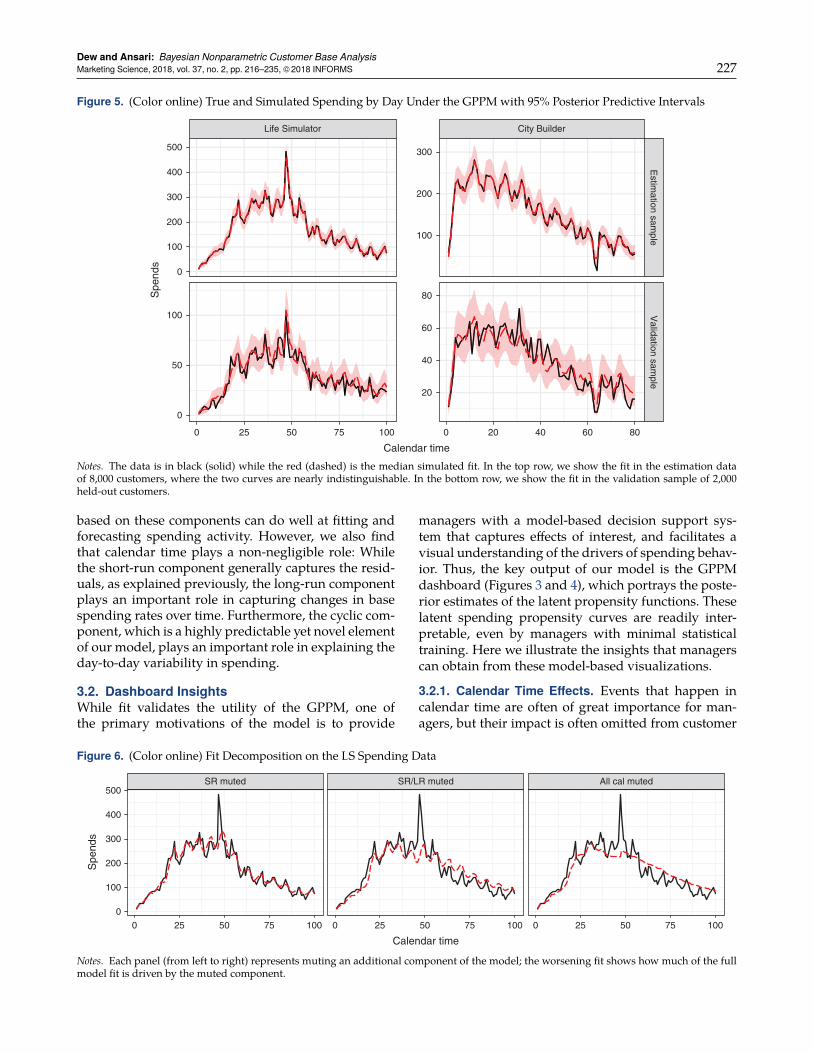
3.1.2. Fit Decomposition. To better understand howthe latent curves in the dashboard contribute to the fitsseen in Figure 5, we now break down that fit along ourlatent dimensions, focusing on the LS game. Our mainfocus is assessing how much of the day-to-day spend-ing is explained by the calendar time components ofthe model versus the typically smoother, individual-level recency, lifetime, and purchase number compo-nents. To do that, we examine how the fit changeswhen different components of the model are muted.Wemute a component by replacing it with a scalar thatis equal to the average of its function values over all itsinputs. Note that we do not reestimate a model whenwe mute a component; instead, muting allows us tosee how much of the overall fit is driven by a givencomponent.
The fit decomposition is shown in Figure 6. Over-laid on the true spending time series, we have threemuted fits: In the first, we mute the short-run calen-dar time component; in the second, we mute the short-and long-run calendar time components; in the third,we mute all calendar time components. From the con-tinued good fit of the muted models, we can see thatthe majority of the full model fit is actually driven bythe individual-level spending predictors, i.e., recency,lifetime, and purchase number. This finding is largelyin keeping with the established literature on customerbase analysis, which has robustly shown that models
Dew and Ansari: Bayesian Nonparametric Customer Base AnalysisMarketing Science, 2018, vol. 37, no. 2, pp. 216–235, ©2018 INFORMS 227
Figure 5. (Color online) True and Simulated Spending by Day Under the GPPM with 95% Posterior Predictive Intervals
Life Simulator
0
100
200
300
400
500
0
50
100
0 25 50 75 100
Spe
nds
City Builder
100
200
300
20
40
60
80
Estim
ation sample
Validation sam
ple
0 20 40 60 80
Calendar time
Notes. The data is in black (solid) while the red (dashed) is the median simulated fit. In the top row, we show the fit in the estimation dataof 8,000 customers, where the two curves are nearly indistinguishable. In the bottom row, we show the fit in the validation sample of 2,000held-out customers.
based on these components can do well at fitting andforecasting spending activity. However, we also findthat calendar time plays a non-negligible role: Whilethe short-run component generally captures the resid-uals, as explained previously, the long-run componentplays an important role in capturing changes in basespending rates over time. Furthermore, the cyclic com-ponent, which is a highly predictable yet novel elementof our model, plays an important role in explaining theday-to-day variability in spending.
3.2. Dashboard InsightsWhile fit validates the utility of the GPPM, one ofthe primary motivations of the model is to provide
Figure 6. (Color online) Fit Decomposition on the LS Spending Data
SR muted SR/LR muted All cal muted
0
100
200
300
400
500
0 25 50 75 100 0 25 50 75 100 0 25 50 75 100
Calendar time
Spe
nds
Notes. Each panel (from left to right) represents muting an additional component of the model; the worsening fit shows how much of the fullmodel fit is driven by the muted component.
managers with a model-based decision support sys-tem that captures effects of interest, and facilitates avisual understanding of the drivers of spending behav-ior. Thus, the key output of our model is the GPPMdashboard (Figures 3 and 4), which portrays the poste-rior estimates of the latent propensity functions. Theselatent spending propensity curves are readily inter-pretable, even by managers with minimal statisticaltraining. Here we illustrate the insights that managerscan obtain from these model-based visualizations.
3.2.1. Calendar Time Effects. Events that happen incalendar time are often of great importance for man-agers, but their impact is often omitted from customer

Dew and Ansari: Bayesian Nonparametric Customer Base Analysis228 Marketing Science, 2018, vol. 37, no. 2, pp. 216–235, ©2018 INFORMS
base analysis models. The GPPM includes these effectsnonparametrically through the calendar time compo-nents of the model, such that the impact of calen-dar time events is captured flexibly and automatically.Calendar time effects are jointly estimated with theindividual-level drivers of spending, recency, lifetime,and purchase number. This means the impact of cal-endar time on spending propensity is assessed onlyafter controlling for these drivers of re-spend behav-ior, which account for the natural ebb and flow ofspending, including dynamics in the numbers of activecustomers.Significantly, capturing the impact of calendar time
events requires no inputs from the marketing analyst,as would be required in a model where time-varyingcovariates are explicitly specified. This implies thattheir presence and significance must be evaluated expost facto. This hasmany benefits: First, even in the faceof information asymmetries or unpredictable shocks,the events will be captured by the GPPM. Second,the shape of the impact of these events is automat-ically inferred, rather than assumed. Finally, becausethe impact is captured by changes in the calendar timecomponents of the propensity model, their impact canbe visually assessed. We demonstrate the analysis ofcalendar time events using our two focal games. Thetop row of plots in each dashboard (Figures 3 and 4,colored blue) represents the calendar time effects. Fromleft to right, we have the long-run trends, short-runshocks, and periodic day of the week effects. Beneaththese curves, we have placed bars indicating time peri-ods of interest to the company.Life Simulator Events. Two events of note occurred inthe span of the data. The first marked time period,t ∈ [17, 30], corresponds to a period in which the com-pany made a game update, introduced a new gametheme involving a color change, and donated all pro-ceeds from the purchases to a charitable organiza-tion. The second marked period, around t ∈ [37, 49],corresponds to another game update that added aChristmas-themed quest to the game, with Christmasitself falling at t � 48, right before the end of the holidayquest.From the dashboard in Figure 3, we learn several
things: First, there is a prominent spike in short-runspending the day before Christmas. This Christmas Eveeffect illustrates that events do not have to be antic-ipated to be detected in the model; below we illus-trate how the GPPM parses out the impact of short-runevents, using this effect as the example. In the long-run curve, we see a decrease in spending coincidingwith the charity update, an increase in spending coin-ciding with the holiday event, and then a significantdrop-off subsequent to the holiday season. Without alonger range of data, it is hard to assess the meaningof these trends. It does appear that the charity event
lowered spending rates. The impact of the holidays ismore unclear: It could be that the holiday game updateelevated spending, and then as time went on, spend-ing levels returned to normal. Alternatively, spendinglevels could be elevated simply due to the holiday sea-son, with a post-holiday slump that is unrelated to thegame updates. Although we cannot conclusively parseout these stories, we can tell that calendar time dynam-ics are at play, and appear linked to real world shocksand company actions.
City Builder Events. The marked areas of the CB dash-board in Figure 4 correspond to events of interest. Thestart of the data window, t ∈ [1, 6], coincides with thetail end of the holiday season, from December 30 toJanuary 4. Another event begins at t � 63, when thecompany launched a permanent update to the gameto encourage repeat spending. We mark five addi-tional days after that update to signify a time periodover which significant postupdate activity may occur.Finally, at t � 72, there was a crash in the app store.We see, as in the previous game, that the spend-
ing level during the holidays, t ∈ [1, 6], was quite highand subsequently fell dramatically. This lends somecredence to a general story of elevated holiday seasonspending, as there was no game update in CB duringthis time. Spending over the rest of the time period wasrelatively stable. The update that was intended to pro-mote repeat spending had an interesting effect: Therewas an initial drop in spending, most likely caused byreduced playtime on that day because of the need forplayers to update their game or because of an error inthe initial launch of the update. After the update, anuptick in long-run spending is observable, but this wasrelatively short lived. Finally, we find no effect for thesupposed app store crash, which in theory should haveprevented players from purchasing for the duration ofthe crash. It is plausible that the crash was for a shortduration or occurred at a time when players were notplaying.
Day of the Week Effects. Across both games, we notethe significance of the periodic day of the week effect.In both cases, spending propensity varies by day of theweek by a magnitude of 0.3. For comparison, the long-run calendar time effect of LS has a range of 0.5, whilethat of CB has a range of 0.6. Themagnitude of the peri-odic effect serves to re-emphasize a point alreadymadein the fit decomposition: A large amount of the calen-dar time variability in spending can be attributed tosimple predictable cyclic effects, something customerbase models have previously ignored, but that can bepowerful in forecasting future purchase behavior.
3.2.2. Event Detection. Often, calendar time eventsare unknown a priori, but can significantly affect con-sumers’ spending rates in the short run. The short-run

Dew and Ansari: Bayesian Nonparametric Customer Base AnalysisMarketing Science, 2018, vol. 37, no. 2, pp. 216–235, ©2018 INFORMS 229
Figure 7. (Color online) Event Detection in the GPPM
Data through 12/23 Data through 12/24 Data through 12/25
−1.8
−1.6
−1.4
−0.2
0
0.2
0.4
LongS
hort
10 15 20 25 10 15 20 25 10 15 20 25
Calendar time
Effe
ct
Note. From left to right, we add daily data, and see how the impact of Christmas Eve is separated between the long-run (top, red) and short-run(bottom, blue) calendar time curves.
function can automatically detect and isolate these dis-turbances. That is, if something disrupts spending for aday, such as a crash in the payment processing system,or an in-game event, it will be reflected as a trough ora spike in the short-run function, as evident, for exam-ple, in the Christmas Eve effect in LS. In this section,we illustrate how this works in practice.
The GPPM estimation process decomposes the cal-endar time effect along subfunctions with differinglength-scales. As such, when there is a disturbance,the GPPM must learn the relevant time scale for thedeviation (here, short or long term) and then adjustaccordingly. We illustrate this dynamically unfoldingadjustment process for the LS Christmas Eve effect inFigure 7 by estimating the model using progressivelymore data from December 23, 2014 to December 25,2014. The different columns show how the long-run(top row) and the short-run (bottom row) componentsvary when data from each successive day is integratedinto the analysis. The second column shows the impactof adding the data from Christmas Eve. An uptick inspending is apparent, but the GPPM cannot yet detectwhether this uptick will last longer or just fade away.The day after (third column), it becomes clear fromlooking at the long-run and short-run plots that theeffect was only transient, which is clearly reflected inthe short-run curve.
This example illustrates that the GPPM can captureeffects of interest with no input from the analyst, andthat the nature of this effect is visually apparent in themodel-based dashboard within days of its occurrence.Note that, significantly, each column of Figure 7 rep-resents a re-estimation of the GPPM, using the pastday’s data; event detection can only occur at the levelof aggregation of the data (in this case, daily), upon re-estimation of the model. Nonetheless, this capabilitycan be immensely valuable to managers in multiprod-uct firms where information asymmetries abound.For example, in digital contexts, product changes cansometimes be rolled out without the knowledge of
the marketing team. Similarly, disruptions in the dis-tribution chain can occur with little information fil-tering back to marketing managers. The GPPM canquickly and automatically capture the impact of suchevents, isolate them from the more regular, predictabledrivers of spending, and bring them to the attention ofmanagers.3.2.3. Individual-Level Effects. While the inclusion ofcalendar time effects is a key innovation in our model,the primary drivers of respend behavior are theindividual-level recency, lifetime, and purchase num-ber effects. We can see this through the fit decomposi-tion, where much of the variability in spending is cap-tured even when the calendar time effects are muted,and also by assessing the range of the effects in thedashboard. As mentioned in Section 2.2, the range ofrelevant inputs in an inverse logit framework is from−6 to 6. For propensity values α < −6, the respendprobability given by logit−1(α) is approximately 0. Sim-ilarly, for propensity values α > 6, the respend proba-bility is approximately 1. This gives an interpretabilityto the curves in the dashboard, as their sum deter-mines this propensity, and hence their range deter-mines how much a given component of the model canalter expected respend probability. Relative to the cal-endar time effects, we can see in the dashboard that theranges of the individual-level effects are significantlylarger, implying that they explain much more of thedynamics in spending propensity than the calendartime components.Recency and Lifetime. In both of our applications, therecency and lifetime effects are smooth and decreas-ing as expected. For managers, this simply means thatthe longer someone goes without spending, and thelonger someone has been a customer in these games,the less likely that person is to spend. The recency effectis consistent with earlier findings and intuitively indi-cates that if a customer has not spent in a while, sheis probably no longer a customer. The lifetime effect is

Dew and Ansari: Bayesian Nonparametric Customer Base Analysis230 Marketing Science, 2018, vol. 37, no. 2, pp. 216–235, ©2018 INFORMS
also expected, especially in the present context, as cus-tomers are more likely to branch out to other games,with the passage of time. More interesting are the ratesat which these decays occur, and how they vary acrossthe games. These processes appear to be fundamen-tally different in the two games. In LS, the recency effecthas a large impact, whereas the lifetime effect assumesa minimal role. By contrast, in CB, both appear equallyimportant. These results may be a result of, for exam-ple, the design of the product (game), which encour-ages a certain pattern of purchasing.Purchase Number. The purchase number effect alsoappears different across the games. In LS, the effectseems relatively insignificant: Although there is aslight rise initially, it quickly evens out, with a largeconfidence interval. In CB, the effect appears quite sig-nificant: It is generally increasing, but appears to flattenout toward the end. The effect in CB is more consis-tent with our expectations: Significant past purchas-ing should indicate a loyal customer, and a likely pur-chaser. A mild or neutral effect, as seen in LS, mayindicate decreasing returns to spending in the game,or a limited number of new items that are available forpurchase, such that the customer quickly runs out ofworthwhile purchase opportunities.Behavioral Implications. The shapes of these curveshave implications for player behavior and for designinggeneral CRM strategies. In LS, the recency effect is theprimary predictor of churn: If a customer has not spentfor a while, she is likely to no longer be a customer.On the other hand, the lifetime effect seems to oper-ate only in the first few days of being a customer, andthen levels out. This implies that customers are mostlikely to spend when they are new to the game, withinroughly two weeks of their first purchase. By contrast,
Figure 8. (Color online) Respend Probability Heat Maps for a Customer with q � 3 and δi � 1
Life Simulator City Builder
10
20
30
40
50
0 10 20 30 40 50 0 10 20 30 40 50
Recency
Life
time
0.25
0.50
0.75
Prob
Notes. Colors represent the probability of respending in the next 100 days, given the current recency and lifetime values. Note that some pairsof recency and lifetime values displayed in the plot are not realistic: A customer cannot have recency higher than lifetime.
in CB, the effects are more equal in magnitude, andmore gradual. The customers who are least likely tospend again are those that have been customers thelongest, and have gone the longest without spending.
We illustrate these differences via an individual-levelanalysis of respend probability. Specifically, we ask:Given an individual’s recency and lifetime, what is theprobability that she spends again in the next 100 days?To carry out this simulation, we fix the calendar timeeffect to its average value, and assume that the indi-vidual has already spent three times. The results of thesimulation are shown in Figure 8, and re-emphasize thepoint that recency explains much of the respend prob-ability in LS, while lifetime and recency are both rele-vant in CB. This analysis also emphasizes the idea that,while the dynamic effects in the GPPM are the samefor all customers, different positions in the individual-level subspace (ri j , li j , pi j) are associated with very dif-ferent expected future purchasing behavior.
In summary, we have seen that the GPPM weavestogether the different model components in a discretehazard framework, and offers a principled approachfor explaining aggregate purchase patterns based onindividual-level data. The model-based dashboard ge-nerated by the GPPM is not the result of ad hocdata smoothing, but arises from the structural decom-position of spending propensity via the differentmodel components. The GPPM jointly accounts for thepredictable individual-level determinants of respendprobability, such as recency, lifetime, and purchasenumber, and calendar time events along multiplelength-scales of variation. Therefore, it can flexibly rep-resent the nature of customer respend probability, andaccurately portray the existence and importance of cal-endar time events and trends.

Dew and Ansari: Bayesian Nonparametric Customer Base AnalysisMarketing Science, 2018, vol. 37, no. 2, pp. 216–235, ©2018 INFORMS 231
3.3. Predictive Ability and Model ComparisonApart from interest in understanding past spendingdynamics, managers also need to forecast future pur-chasing activity. Although the primary strength of theGPPM is in uncovering latent dynamics, and intu-itively conveying them through the model-based dash-board, the GPPM also does very well in predictingfuture spending. Just as in-sample fit was driven bythe recency, lifetime, and purchase number compo-nents, predictive performance depends primarily onthe ability to forecast these components for observa-tions in the holdout data. While forms of recency, life-time, and purchase number effects are incorporatedin most customer base models, the isolation of theseeffects apart from transient calendar time variability,along with nonparametric characterization of thesepredictable components, and the inclusion of the cycliccomponent, allow the GPPM to significantly outper-form benchmark customer base analysis models in pre-dictive ability.In this section, we focus on comparing model fit
and future predictive performance, and therefore rees-timate the GPPM by truncating our original calibra-tion data of 8,000 customers along the calendar timedimension. In particular, we set aside the last 30 days ofcalendar time activity to test predictive validity. Fore-casting with the GPPM involves forecasting the latentfunctions that comprise it. In forecasting these latentfunctions, we use the predictive mechanisms outlinedin Section 2.1 (Equation (4)). As the holdout data isconstructed by splitting the original data set alongthe calendar time dimension, a substantial number ofobservations in the holdout data contain recency, life-time, and purchase number values that are within theobservable range of these variables in the calibrationdata set. This is especially true for observations belong-ing to newly acquired customers. However, for the old-est customers, the individual-level curves need to beforecast.
3.3.1. Benchmark Models. We compare the predictiveperformance of the GPPM with that of a numberof benchmark models. Many individual-level modelshave been developed to perform customer base anal-ysis. At its core, the GPPM is a very general discretehazard model and, as such, can be compared to otherhazard models for interpurchase times (Gupta 1991,Seetharaman and Chintagunta 2003). Similarly, givenits reliance on recency, lifetime, and purchase numberdimensions of spending, the GPPM is closely relatedto traditional customer base analysis models for non-contractual settings in the BTYD vein (Schmittlein et al.1987; Fader et al. 2005, 2010). Finally, the discrete haz-ard approach could be modified with a different spec-ification of the spend propensity.
Hazard Models. We consider two standard discretizedhazard models, i.e., the Log-Logistic model and the Log-Logistic Covmodel, which are standard log-logistic haz-ard models without and with time-varying covariates,respectively. We choose the log-logistic hazard as it canflexibly represent monotonic and nonmonotonic haz-ard functions. In the model with covariates, we useindicator variables over the time periods of interest asindicated at the start of Section 3. In estimating bothof these models, we use the same Bayesian estimationstrategy, using Stan, with the same random effect het-erogeneity specification as in the GPPM.BTYD. We use the Pareto-NBD (Schmittlein et al. 1987)and the BG/NBD (Fader et al. 2010) as benchmarks inthis class. While many variants of BTYD have beendeveloped over the years, the Pareto-NBD has stoodthe test of time as the gold standard in forecastingpower in noncontractual settings, often beating evenmore recent models (see, e.g., the PDOmodel in Jerathet al. 2011). The BG/NBD is a more discrete analogueof the Pareto-NBD, where customer death can occurafter each purchase, rather than continuously.10
Propensity Models. In this case, we retain the dis-crete time hazard inverse logit framework, while alter-ing the specification of the dynamics. In particular,we explore two specifications, i.e., the Linear Propen-sity Model (LPM) and the State Space Propensity Model(SSPM). To our knowledge, these models have notbeen explored elsewhere in the literature; we includethem here to help understand the benefits of the GPapproach to modeling dynamics.
In the LPM, we remove the nonparametric spec-ification, and instead model all effects linearly, asPr(yi j � 1) � logit−1(µ + β1ti j + β2ri j + β3li j + β4qi j + δi).This is the simplest discrete hazardmodel specificationthat includes all of our time scales and effects.
In the SSPM, we explore an alternate nonparamet-ric specification for the dynamic effects. There are anumber of competing nonparametric function estima-tion techniques, including dynamic linear models andvarious spline specifications, and there are technicallinks between many of these modeling approaches.Moreover, in each class of models, a range of spec-ifications are possible, making the choice of a suit-able benchmark difficult. We implement a state spacespecification roughly equivalent to the GP structurein our main model. Specifically, we decompose thepropensity function α(t , r, l , q) into additive compo-nents along each dimension. For the calendar timedimension, just as in the GPPM, we make no assump-tions about its behavior, and hence model it as a ran-dom walk
αT(t)� αT(t − 1)+ εTt , εTt ∼N (0, ζ2T). (11)
For the other dimensions, we assume, as in the GPPM,that there will likely be monotonicity, and hence
Dew and Ansari: Bayesian Nonparametric Customer Base Analysis232 Marketing Science, 2018, vol. 37, no. 2, pp. 216–235, ©2018 INFORMS
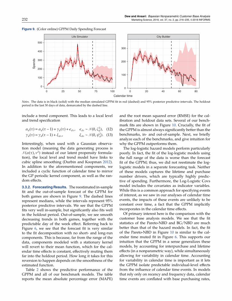
Figure 9. (Color online) GPPM Daily Spending Forecast
Life Simulator City Builder
0
100
200
300
400
500
0
100
200
300
0 25 50 75 100 0 20 40 60 80
Calendar time
Spe
nds
Notes. The data is in black (solid) with the median simulated GPPM fit in red (dashed) and 95% posterior predictive intervals. The holdoutperiod is the last 30 days of data, demarcated by the dashed line.
include a trend component. This leads to a local leveland trend specification
αd(τ)� αd(τ− 1)+ γd(τ)+ εdτ , εdτ ∼N (0, ζ2d), (12)
γd(τ)� γd(τ− 1)+ ξdτ , ξdτ ∼N (0, ψ2d). (13)
Interestingly, when used with a Gaussian observa-tion model (meaning the data generating process isN (α(τ), ν2) instead of our latent propensity formula-tion), the local level and trend model have links tocubic spline smoothing (Durbin and Koopman 2012).In addition to the aforementioned components, weincluded a cyclic function of calendar time to mirrorthe GP periodic kernel component, as well as the ran-dom effects.
3.3.2. ForecastingResults. The reestimated in-samplefit and the out-of-sample forecast of the GPPM forboth games are shown in Figure 9. The dashed linesrepresent medians, while the intervals represent 95%posterior predictive intervals. We see that the GPPMfits very well in-sample, but significantly also fits wellin the holdout period. Out-of-sample, we see smoothdecreasing trends in both games, together with thepredictable day of the week effect. Referring back toFigure 6, we see that the forecast fit is very similarto the fit decomposition with no short- and long-runcomponents. This is because, far from the range of thedata, components modeled with a stationary kernelwill revert to their mean function, which for the cal-endar time effects is constant, effectively muting themfar into the holdout period. How long it takes for thisreversion to happen depends on the smoothness of theestimated function.Table 2 shows the predictive performance of the
GPPM and all of our benchmark models. The tablereports the mean absolute percentage error (MAPE)
and the root mean squared error (RMSE) for the cal-ibration and holdout data sets. Several of our bench-mark fits are shown in Figure 10. Crucially, the fit ofthe GPPM is almost always significantly better than thebenchmarks, in- and out-of-sample. Next, we brieflyanalyze each of the benchmarks, and give intuition forwhy the GPPM outperforms them.
The log-logistic hazard models perform particularlypoorly. In fact, the fit of the log-logistic models usingthe full range of the data is worse than the forecastfit of the GPPM; thus, we did not reestimate the log-logistic models in a separate forecasting task. Neitherof these models captures the lifetime and purchasenumber drivers, which are typically highly predic-tive of spending. Furthermore, the Log-Logistic Covsmodel includes the covariates as indicator variables.While this is a common approach for specifying eventsof interest, as we saw in our analyses of calendar timeevents, the impacts of these events are unlikely to beconstant over time, a fact that the GPPM implicitlyincorporates in the calendar time effects.
Of primary interest here is the comparison with thecustomer base analysis models. We see that the fitstatistics of the Pareto-NBD and BG/NBD are muchbetter than that of the hazard models. In fact, the fitof the Pareto-NBD in Figure 10 is similar to the cal-endar time muted fit in Figure 6. This supports ourintuition that the GPPM in a sense generalizes thesemodels, by accounting for interpurchase and lifetimeeffects (in a nonparametric way), while simultaneouslyallowing for variability in calendar time. Accountingfor variability in calendar time is important as it letsthe GPPM isolate predictable individual-level effectsfrom the influence of calendar time events. In modelsthat rely only on recency and frequency data, calendartime events are conflated with base purchasing rates,
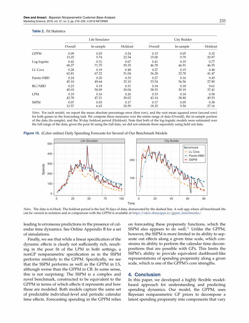
Dew and Ansari: Bayesian Nonparametric Customer Base AnalysisMarketing Science, 2018, vol. 37, no. 2, pp. 216–235, ©2018 INFORMS 233
Table 2. Fit Statistics
Life Simulator City Builder
Overall In-sample Holdout Overall In-sample Holdout
GPPM 0.09 0.03 0.24 0.15 0.05 0.3213.25 5.74 22.54 15.00 9.79 20.97
Log-logistic 0.42 0.31 0.67 0.41 0.19 0.7768.27 71.75 59.35 46.78 46.91 46.55
LL Covs 0.28 0.19 0.48 0.27 0.15 0.4862.81 67.22 51.04 36.28 32.78 41.47
Pareto-NBD 0.24 0.20 0.33 0.27 0.16 0.4545.10 49.64 32.10 33.54 36.56 27.80
BG/NBD 0.23 0.19 0.31 0.34 0.18 0.6145.03 50.09 30.04 38.53 39.19 37.41
LPM 0.19 0.16 0.26 0.33 0.18 0.5842.78 47.21 30.02 43.14 38.80 49.53
SSPM 0.07 0.03 0.17 0.17 0.05 0.3812.57 6.63 20.59 18.25 9.50 27.16
Notes. For each model, we report the mean absolute percentage error (first row), and the root mean squared error (second row)for both games in the forecasting task. We compute these measures over the entire range of data (Overall), the in-sample portionof the data (In-sample), and the 30-day holdout period (Holdout). Note that both of the log-logistic models were estimated overthe full range of the data; given the poor fit using the full data, we did not estimate them separately using held out data.
Figure 10. (Color online) Daily Spending Forecasts for Several of Our Benchmark Models
Life Simulator City Builder
0
100
200
300
400
500
100
200
0 25 50 75 100 0 20 40 60 80
Time
Spe
nds
Benchmark
LL CovsPareto-NBDSSPM
Notes. The data is in black. The holdout period is the last 30 days of data, demarcated by the dashed line. A web app where all benchmark fitscan be viewed in isolation and in comparison with the GPPM is available at https://rdew.shinyapps.io/gppm_benchmarks/.
leading to erroneous predictions in the presence of cal-endar time dynamics. See Online Appendix B for a setof simulations.Finally, we see that while a linear specification of the
dynamic effects is clearly not sufficiently rich, result-ing in the poor fit of the LPM in both settings, anonGP nonparametric specification as in the SSPMperforms similarly to the GPPM. Specifically, we seethat the SSPM performs as well as the GPPM in LS,although worse than the GPPM in CB. In some sense,this is not surprising: The SSPM is a complex andnovel benchmark, constructed to be equivalent to theGPPM in terms of which effects it represents and howthese are modeled. Both models capture the same setof predictable individual-level and periodic calendartime effects. Forecasting spending in the GPPM relies
on forecasting these propensity functions, which theSSPM also appears to do well.11 Unlike the GPPM,however, the SSPM is more limited in its ability to sep-arate out effects along a given time scale, which con-strains its ability to perform the calendar time decom-positions that are possible with GPs. This limits theSSPM’s ability to provide equivalent dashboard-likerepresentations of spending propensity along a givenscale, which is one of the GPPM’s core strengths.
4. ConclusionIn this paper, we developed a highly flexible model-based approach for understanding and predictingspending dynamics. Our model, the GPPM, usesBayesian nonparametric GP priors to decompose alatent spending propensity into components that vary

Dew and Ansari: Bayesian Nonparametric Customer Base Analysis234 Marketing Science, 2018, vol. 37, no. 2, pp. 216–235, ©2018 INFORMS
along calendar time, interpurchase time, customer life-time, and purchase number dimensions. Our additivestructure yields easily interpretable model outputs andfits customer spending data well.We showed that the GPPM identifies the latent
dynamic patterns in the data via a principled proba-bilistic framework that reliably separates signal fromnoise. It offers a number of outputs that are ofconsiderable value to managers. First, the GPPM gen-erates a dashboard of latent functions that character-ize the spending process. These model-based visual-izations are easy to comprehend, even by managerswho may lack sophisticated statistical skills. Second,we demonstrated that the GPPM is capable of auto-matically capturing the effect of events that may beof interest to managers. In situations where certainevents may escape the notice of managers, the GPPMautomatically detects these events. More important,the nonparametric nature of the GPPM allows it toflexibly model the nature and duration of the impactof events (known or unknown, a priori), without theneed to represent these explicitly via covariates. Theseadvantages of the GPPM make it ideal for decisioncontexts involving multiple products and informationasymmetries. The GPPM also flexibly captures theindividual-level spending drivers that reliably explainand predict spending behavior, including recency, life-time, and purchase number effects. These effects can beused to characterize spending patterns within distinctcustomer bases, analyze individual customer respendprobabilities, and predict future spending activity. Fur-thermore, since these effects are jointly estimated withthe calendar time events, as part of a unified propen-sity model, the predictable, fundamental individual-level spending drivers are determined net of poten-tially unpredictable calendar time effects. Moreover,calendar time events can be analyzed net of the impactof expected individual-level spending activity, in a waynot possible with mere aggregate data analysis.
We demonstrated these benefits of the GPPM on twodata sets of purchasing activity within mobile games.We illustrated how themodel-based dashboards gener-ated from the GPPM yield easily interpretable insightsabout fundamental patterns in purchasing behavior.We also showed that the GPPM outperforms tra-ditional customer base analysis models in terms ofpredictive performance, both in-sample and out-of-sample, including hazard models with time-varyingcovariates and the class of BTYD models. The predic-tive superiority of the GPPM stems from the fact thatit captures the same predictable effects as traditionalcustomer base analysis models, such as recency andlifetime, but does so in a flexible way, net of the influ-ence of calendar time events.
While this paper showcases the many benefits ofour framework, it is also important to acknowledge
some limitations. First, the framework in its currentform is computationally demanding, especially whencompared with simpler probability models that canbe estimated with maximum likelihood. It is alsodata intensive. In our application, we used completeindividual-level event log data to estimate the model.Some of the benchmark models, in particular, theBG/NBD and the Pareto-NBD, use only two sufficientstatistics per customer. Both of these limitations canperhaps be addressed in practice by data subsampling,or by developing faster inference algorithms. Finally,while we believe our model-based dashboard is useful,insofar as it provides a snapshot of the key drivers ofspending dynamics, it does not work in real-time, asis the case for many dashboards of marketing metrics.A streaming data version of our model would be aninteresting area for future work.
To conclude, we believe the GPPM addresses a fun-damental need of modern marketing managers for aflexible system for dynamic customer base analysis. Inproviding a solution to this problem, this work intro-duces a new Bayesian nonparametric approach to themarketing literature. While we discuss GP priors in thecontext of dynamic customer base analysis, their poten-tial applicability to other areas of marketing is muchbroader. GPs provide a general mechanism for flexi-bly modeling unknown functions, and for a Bayesiantime series analysis. We see many potential applica-tions for GPs in marketing, including modeling of theimpact of marketing mix variables, such as advertisingand promotions, and approximation of unknown func-tions in dynamic programming and other simulationcontexts. Our work also makes a contribution to thelargely unaddressed field of visual marketing analyt-ics systems, or dashboards. Dashboards and market-ing analytics systems are likely to become even moreimportant in the future, given the increasing complex-ity of modern data-rich environments. As dashboardsincrease in relevance, we believe that managers willwelcome further academic research in this domain.
AcknowledgmentsThe authors thank the review team for their insightful com-ments and suggestions.
Endnotes1Hereafter, we use the words purchasing and spending interchange-ably to refer specifically to purchase incidence.2This behavior can be seen through Equation (4), in conjunc-tion with, for example, the SE kernel, which has functional formkSE(τi , τ j) � η2 exp{−(τi − τ j)2/(2ρ2)}. As the distance between theobserved inputs and the new input grows, the value of the kernelgoes to zero, and we see that the mean in Equation (4) will revertto the mean function. This mean reverting property depends on thekernel being stationary, meaning that it depends only on the distancebetween inputs. See Rasmussen and Williams (2006) for a compre-hensive discussion of these issues.

Dew and Ansari: Bayesian Nonparametric Customer Base AnalysisMarketing Science, 2018, vol. 37, no. 2, pp. 216–235, ©2018 INFORMS 235
3We note that the properties of this specification are suitable for ourspecific application, but may not be suitable in other domains andsubstantive applications.4 In general, determining the number of additive components suit-able for a given application requires substantive knowledge andexpectations about the nature of the dynamics at work, and data-driven evidence from the estimated hyperparameter values. Forinstance, depending on the kernel, a small amplitude hyperparam-eter compared to the output scale could indicate that the compo-nent is relatively uninfluential in describing the results. Similarly, ifthe length-scale is estimated to be very large, this can indicate thatminimal dynamics are being uncovered by that component. Both ofthese phenomena can indicate redundancy in the specification. Ker-nel specification is a rich topic in the GP literature; see Rasmussenand Williams (2006), Chapter 5 for a detailed discussion.5While we emphasize the relative benefits of GP priors here, we alsonote that there are many links between these methods, includingbetween GP methods and smoothing splines (Kalyanam and Shively1998 andShively et al. 2000), andbetweenGPmethods and state spacemodels.We include a sophisticated state space analog of ourmodel inour benchmarks. Our state space formulation is also closely related tocubic spline specifications (seeDurbinandKoopman2012 fordetails).As we describe in Section 3.3.2, although this method produces fitsthat are roughly onparwith theGPapproach,we cannot easily obtainthe decompositions that are natural in the GP setting.6See Online Appendix B for simulated data examples of these effects,where we know the effects true forms, and can show that the GPPMis capable of accurately recovering them.7We may not expect this in our application area, freemium videogames, where there can be decreasing returns to repeat purchasing.8See Online Appendix C for our Stan code.9There is no personally identifiable information in our data; playerinformation is masked such that none of the data we use or theresults we report can be traced back to the actual individuals. Wealso mask the identification of the company as per their request.10We estimate these models using the BTYD package in the R pro-gramming language.11 In fact, recent research has established deep links between GPsand state space models, such that some GP models can be approxi-mated by state-space specifications (Gilboa et al. 2015). This may alsoexplain their similar performance.
ReferencesAnsari A, Mela CF (2003) E-customization. J. Marketing Res. 40(2):
131–145.Carpenter B, Gelman A, Hoffman M, Lee D, Goodrich B, Betancourt
M, Brubaker MA, Li P, Riddell A (2017) Stan: A probabilisticprogramming language. J. Statist. Software 20:1–37.
Durbin J, Koopman SJS (2012) Time Series Analysis by State Space Meth-ods, 2nd ed. (Oxford University Press, Oxford, UK).
DuvenaudD, Lloyd J, Grosse R, Tenenbaum J, Zoubin G (2013) Struc-ture discovery in nonparametric regression through composi-tional kernel search. Dasgupta S, McAllester D, eds. Proc. 30thInternat. Conf. Machine Learn., Vol. 28, 1166–1174.
Fader P, Hardie B, Lee KL (2005) Counting your customers the easyway: An alternative to the Pareto/NBD model. Marketing Sci.24(2):275–284.
Fader P, Hardie B, Shang J (2010) Customer-base analysis ina discrete-time noncontractual setting. Marketing Sci. 29(6):1086–1108.
GelmanA, Rubin DB (1992) Inference from iterative simulation usingmultiple sequences. Statist. Sci. 7(4):457–511.
Gilboa E, Saatci Y, Cunningham JP (2015) Scaling multidimensionalinference for structured Gaussian processes. IEEE Trans. PatternAnal. Machine Intelligence 37(2):424–436.
Gupta S (1991) Stochastic models of interpurchase time with time-dependent covariates. J. Marketing Res. 28(1):1–15.
Hanssens DM, Parsons LJ, Schultz RL (2001) Market Response Models:Econometric and Time Series Analysis, 2nd ed. (Kluwer AcademicPublishers, Norwell, MA).
Hoffman M, Gelman A (2014) The no-U-turn sampler: Adaptivelysetting path lengths in Hamiltonian Monte Carlo. J. MachineLearn. Res. 15(1):1351–1381.
Jerath K, Fader PS, Hardie BG (2011) New perspectives on customerdeath using a generalization of the Pareto/NBD model. Market-ing Sci. 30(5):866–880.
Kalyanam K, Shively TS (1998) Estimating irregular pricing effects:A stochastic spline regression approach estimating irregularpricing effects: A stochastic spline regression approach. J. Mar-keting Res. 35(1):16–29.
Kim JG, Menzefricke U, Feinberg FM (2007) Capturing flexible het-erogeneous utility curves: A Bayesian spline approach. Manage-ment Sci. 53(2):340–354.
Li Y, Ansari A (2014) A Bayesian semiparametric approach for endo-geneity and heterogeneity in choice models. Management Sci.60(5):1161–1179.
Neal RM (1998) Regression and classification using Gaussian processpriors. Bernardo JM, ed. Bayesian Statistics 6 (Oxford UniversityPress, Oxford, UK), 475–501.
Neslin SA, Gupta S, Kamakura W, Lu J, Mason CH (2006) Defec-tion detection: Measuring and understanding the predictiveaccuracy of customer churn models. J. Marketing Res. 43(2):204–211.
Pauwels K, Ambler T, Clark BH, LaPointe P, Reibstein D, Skiera B,Wierenga B, Wiesel T (2009) Dashboards as a service: Why,what, how, and what research is needed? J. Service Res. 12(2):175–189.
Rasmussen E,WilliamsKI (2006)Gaussian Processes for Machine Learn-ing (MIT Press, Cambridge, MA).
Roberts S, Osborne M, Ebden M, Reece S, Gibson N, Aigrain S (2013)Gaussian processes for time-series modelling. Philos. Trans. Ser.A, Math., Phys., Engrg. Sci. 371(1984):20110550.
Rossi PE (2014) Bayesian Non- and Semi-Parametric Methods and Appli-cations, Econom. Tinbergen Institutes Lectures (Princeton Uni-versity Press, Princeton, NJ).
Schmittlein DC,Morrison DG, Colombo R (1987) Counting your cus-tomers: Who-are they and what will they do next? ManagementSci. 33(1):1–24.
Schweidel DA, Knox G (2013) Incorporating direct marketing activityinto latent attrition models. Marketing Sci. 32(3):471–487.
Seetharaman PB, Chintagunta PK (2003) The proportional hazardmodel for purchase timing: A comparison of alternative specifi-cations. J. Bus. Econom. Statist. 21(3):368–382.
Shively TS, AllenbyGM, Kohn R (2000) A nonparametric approach toidentifying latent relationships in hierarchicalmodels.MarketingSci. 19(2):149–162.
Wedel M, Zhang J (2004) Analyzing brand competition across sub-categories. J. Marketing Res. 41(4):448–456.