Embed Size (px)
Citation preview

Basics Loss Functions Quadratic Loss Asymmetirc Linear Loss All-or-nothing Loss Example
Bayesian Point Estimation
Econ 690
Purdue University
Justin L. Tobias Point Estimation
Basics Loss Functions Quadratic Loss Asymmetirc Linear Loss All-or-nothing Loss Example
Outline
1 Basic Framework
2 Common Loss Functions
3 Point Estimation Under Quadratic Loss
4 Point Estimation Under Asymmetric Linear Loss
5 Point Estimation Under All-or-Nothing Loss
6 Example
Justin L. Tobias Point Estimation

Basics Loss Functions Quadratic Loss Asymmetirc Linear Loss All-or-nothing Loss Example
Framework
The Bayesian begins by specifying a loss (cost) function C (θ̂, θ).This is:
1 A nonnegative function satisfying C (θ, θ) = 0.
2 A function that measures the consequences of using θ̂ = θ̂(Y )(i.e., a particular function of the data) as an estimate whenthe “state of nature” is θ.
3 Usually, C (θ̂, θ) is a non-decreasing function of the (absolutevalue of the) sampling error θ̂ − θ.
4 Whether or not to impose symmetry of the sampling erroraround zero is at the discretion of the researcher and willdepend on the problem at hand.
Justin L. Tobias Point Estimation

Basics Loss Functions Quadratic Loss Asymmetirc Linear Loss All-or-nothing Loss Example
Framework
A good estimate is one which “minimizes” C (θ̂, θ) in somesense, but its randomness must first be eliminated.
From the frequentist sampling theory point of view, θ isnon-stochastic but C (θ̂, θ) is nonetheless stochastic becausethe estimator θ̂ = θ̂(Y ) is a random variable.
An obvious way to circumscribe the randomness of C (θ̂, θ) isto focus attention on its expected value. Frequentiststherefore consider the Risk function:
R(θ̂|θ) = EY |θ[C (θ̂(Y ), θ)],
where the expectation (assumed to exist) is taken withrespect to the sampling density p(y |θ).
Justin L. Tobias Point Estimation

Basics Loss Functions Quadratic Loss Asymmetirc Linear Loss All-or-nothing Loss Example
Framework
In contrast the Bayesian perspective is entirely ex post (i.e., itconditions on the observed data y).
That is, the Bayesian uses θ̂ = θ̂(y) as a point estimate of theunknown parameter θ.
The Bayesian solution to the randomness of the loss functionis similar to the frequentist solution: take its expectationbefore minimization.
The expectation, however, is with respect to the posteriordistribution θ|y , and not the sampling distribution y |θ used toobtain the risk function.
Justin L. Tobias Point Estimation
Basics Loss Functions Quadratic Loss Asymmetirc Linear Loss All-or-nothing Loss Example
Framework
The Bayesian point estimate is defined as the solution(assuming the expectation exists) to the following problem:
where
Most importantly, note that the posterior expectation removesθ from the criterion function, unlike the case of risk functionR(θ̂|θ).
Justin L. Tobias Point Estimation

Basics Loss Functions Quadratic Loss Asymmetirc Linear Loss All-or-nothing Loss Example
Framework
Also note that if the researcher is interested only in a subset θ1 ofthe parameter vector θ = [θ1, θ2]′, this preference can be reflectedin the loss function specification: C (θ̂, θ) = C (θ̂1, θ1). In this case:
Thus, nuisance parameters are simply marginalized out of theproblem.
Justin L. Tobias Point Estimation

Basics Loss Functions Quadratic Loss Asymmetirc Linear Loss All-or-nothing Loss Example
Popular Loss (Cost) Functions
Consider the case of a single parameter of interest θ. Let c, c1 andc2 be known constants.
is known as a quadratic loss function.
Justin L. Tobias Point Estimation
Basics Loss Functions Quadratic Loss Asymmetirc Linear Loss All-or-nothing Loss Example
Popular Loss (Cost) Functions
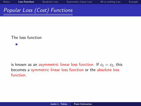
The loss function
is known as an asymmetric linear loss function. If c1 = c2, thisbecomes a symmetric linear loss function or the absolute lossfunction.
Justin L. Tobias Point Estimation
Basics Loss Functions Quadratic Loss Asymmetirc Linear Loss All-or-nothing Loss Example
Popular Loss (Cost) Functions
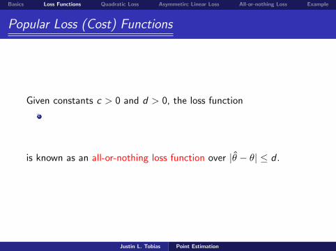
Given constants c > 0 and d > 0, the loss function
is known as an all-or-nothing loss function over |θ̂ − θ| ≤ d .
Justin L. Tobias Point Estimation

Basics Loss Functions Quadratic Loss Asymmetirc Linear Loss All-or-nothing Loss Example
Popular Loss (Cost) Functions
When there are several parameters of interest, the most popularloss functions are of the weighted squared error type:
where Q is a positive definite matrix
Justin L. Tobias Point Estimation

Basics Loss Functions Quadratic Loss Asymmetirc Linear Loss All-or-nothing Loss Example
Loss Functions, Plotted
−2 −1.5 −1 −0.5 0 0.5 1 1.5 2Sampling Error
Quadratic Loss
Linear Loss
All−or−nothing loss
Justin L. Tobias Point Estimation

Basics Loss Functions Quadratic Loss Asymmetirc Linear Loss All-or-nothing Loss Example
Point Estimation under (Weighted) Squared Error Loss
Consider the cost function
C (θ̂, θ) = (θ̂ − θ)′Q(θ̂ − θ)
We can write this as:
Justin L. Tobias Point Estimation

Basics Loss Functions Quadratic Loss Asymmetirc Linear Loss All-or-nothing Loss Example
Point Estimation under (Weighted) Squared Error Loss
Noting that only the last two terms of the previous expressioninvolve θ, the posterior expected loss is
Picking θ̂ = E (θ|y) minimizes this expression. Note that θ̂ doesnot depend on Q.
Justin L. Tobias Point Estimation

Basics Loss Functions Quadratic Loss Asymmetirc Linear Loss All-or-nothing Loss Example
Point Estimation Under Asymmetric Linear Loss
C (θ̂, θ) =
{c1|θ̂ − θ| if θ̂ ≤ θc2|θ̂ − θ| if θ̂ > θ
Before working out the point estimate under this loss function, weneed to recall Leibniz’s Rule (differentiation under the integralsign):
∂
∂x
∫ v(x)
u(x)f (t)dt = f [v(x)]
∂v
∂x− f [u(x)]
∂u
∂x.
Back to derivation
Justin L. Tobias Point Estimation

Basics Loss Functions Quadratic Loss Asymmetirc Linear Loss All-or-nothing Loss Example
Point Estimation Under Asymmetric Linear Loss
C (θ̂, θ) =
{c1|θ̂ − θ| if θ̂ ≤ θc2|θ̂ − θ| if θ̂ > θ
Posterior expected loss is
where P (·) denotes the c.d.f. corresponding to p (·).
Justin L. Tobias Point Estimation

Basics Loss Functions Quadratic Loss Asymmetirc Linear Loss All-or-nothing Loss Example
Point Estimation Under Asymmetric Linear Loss
Eθ|y [C (θ̂, θ)] = c2θ̂P(θ̂|y)− c2
∫ θ̂
−∞θp(θ|y)dθ −
c1θ̂[1− P(θ̂|y)] + c1
∫ ∞θ̂
θp(θ|y)dθ.
Differentiating the above with respect to θ̂ (i.e., applying Leibniz’srule) to Leibniz’s Rule yields
Justin L. Tobias Point Estimation

Basics Loss Functions Quadratic Loss Asymmetirc Linear Loss All-or-nothing Loss Example
Point Estimation Under Asymmetric Linear Loss
∂Eθ|y [C (θ̂, θ)]
∂θ̂= −c1 + (c1 + c2)P(θ̂|y).
Equating this expression to zero and solving for θ̂ yields
θ̂ = P−1θ|y
(c1
c1 + c2
),
i.e., the c1/(c1 + c2) posterior quantile of θ.
Justin L. Tobias Point Estimation

Basics Loss Functions Quadratic Loss Asymmetirc Linear Loss All-or-nothing Loss Example
Point Estimation Under Asymmetric Linear Loss
Note that
If c1 = c2, θ̂ = P−1θ|y (1/2), so that under absolute loss
(symmetric linear loss), the posterior median is the optimalpoint estimate
If c2 is large relative to c1 in the sense that c2 = kc1 for largek, then
θ̂ = P−1θ|y[(1 + k)−1
],
where argument inside the inverse cdf function is a smallnumber, and thus θ̂ moves into the left-tail of p(θ|y).This makes some sense since, in this structure, the relativepenalty for choosing θ̂ to be “too big” has increased. That is,the penalty for overestimation is far greater than that forunderestimation, resulting in “small” θ̂.
Justin L. Tobias Point Estimation

Basics Loss Functions Quadratic Loss Asymmetirc Linear Loss All-or-nothing Loss Example
Point Estimation Under All-or-Nothing Loss
C (θ̂, θ) =
{c if |θ̂ − θ| > d
0 if |θ̂ − θ| ≤ d
Expected posterior loss is
Justin L. Tobias Point Estimation
Basics Loss Functions Quadratic Loss Asymmetirc Linear Loss All-or-nothing Loss Example
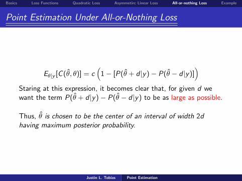
Point Estimation Under All-or-Nothing Loss
Eθ|y [C (θ̂, θ)] = c(
1− [P(θ̂ + d |y)− P(θ̂ − d |y)])
Staring at this expression, it becomes clear that, for given d wewant the term P(θ̂ + d |y)− P(θ̂ − d |y) to be as large as possible.
Thus, θ̂ is chosen to be the center of an interval of width 2dhaving maximum posterior probability.
Justin L. Tobias Point Estimation

Basics Loss Functions Quadratic Loss Asymmetirc Linear Loss All-or-nothing Loss Example
Point Estimation Under All-or-Nothing Loss
Differentiating expected (posterior) loss with respect to θ̂ yields
Equating the above to zero and solving for θ̂ implies the end pointsof this interval have equal posterior density.Also note that as d → 0, θ̂ becomes the mode of p(θ|y).
Justin L. Tobias Point Estimation

Basics Loss Functions Quadratic Loss Asymmetirc Linear Loss All-or-nothing Loss Example
Example with Log Wage Data
Consider again our illustrative example with log wage data.
The data set used contains 1,217 observations on threevariables: hourly wages, education and a standardized testscore.
We consider the model
yi = β0 + β1Edi + εi ,
where y is the log of the hourly wage.
We also employ the flat prior
p(β0, β1, σ2) ∝ σ−2.
Justin L. Tobias Point Estimation

Basics Loss Functions Quadratic Loss Asymmetirc Linear Loss All-or-nothing Loss Example
Example with Log Wage Data
In the slides related to Bayesian inference in the linearregression model, we showed:
β1|y ∼ t(.0910, [.0066]2, 1, 215).
Derive the Bayesian point estimates of the return to educationunder quadratic, asymmetric linear (with c2 = 2c1) andabsolute (as d → 0) losses.
Justin L. Tobias Point Estimation

Basics Loss Functions Quadratic Loss Asymmetirc Linear Loss All-or-nothing Loss Example
Example with Log Wage Data
Under quadratic loss, the optimal point estimate is theposterior mean, E (β1|y). Thus,
β̂1 = .091
is the optimal point estimate under this loss function.
Under all-or-nothing loss, as d → 0, the posterior mode is theoptimal point estimate. Since the Student-t is symmetric withmean, median and mode equal to β̂, it follows that
β̂1 = .091
is again the optimal point estimate under this loss function.
Justin L. Tobias Point Estimation

Basics Loss Functions Quadratic Loss Asymmetirc Linear Loss All-or-nothing Loss Example
Example with Log Wage Data
For the asymmetric linear loss function, with c2 = 2c1, wehave (using crude notation)
β̂1 = T−1ν (β1; 1/3).
In other words, we seek a β̂1 such that
Tν(β̂1; .091, [.0066]2) = 1/3.
[The above notation denotes the Student-t cdf according tothe given mean, variance, and degrees of freedom parameter.]
Justin L. Tobias Point Estimation
Basics Loss Functions Quadratic Loss Asymmetirc Linear Loss All-or-nothing Loss Example
Example with Log Wage Data
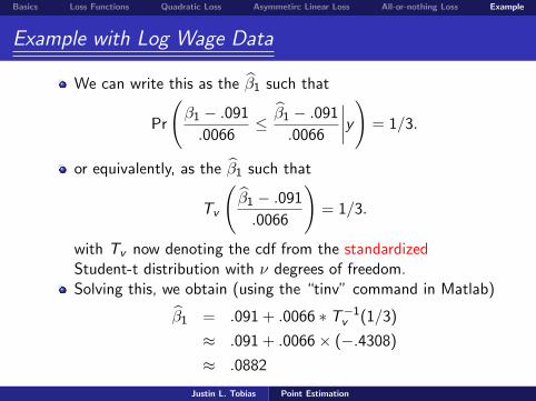
We can write this as the β̂1 such that
Pr
(β1 − .091
.0066≤ β̂1 − .091
.0066
∣∣∣∣y)
= 1/3.
or equivalently, as the β̂1 such that
Tv
(β̂1 − .091
.0066
)= 1/3.
with Tv now denoting the cdf from the standardizedStudent-t distribution with ν degrees of freedom.Solving this, we obtain (using the “tinv” command in Matlab)
β̂1 = .091 + .0066 ∗ T−1v (1/3)
≈ .091 + .0066× (−.4308)
≈ .0882
Justin L. Tobias Point Estimation
Basics Loss Functions Quadratic Loss Asymmetirc Linear Loss All-or-nothing Loss Example
Other Loss Functions
Another possible loss function, though less widely-used, is theLINEX loss function, Varian (1975), Zellner (1986 JASA, “BayesianEstimation and Prediction Using Asymmetric Loss Functions” ):
Note: exp(a∆) ≈ 1 + a∆ + (1/2)a2∆2 and thus, for a ≈ 0,this behaves much like a quadratic loss function.
For a > 0, the exponential term dominates for large ∆,implying that overestimation is more costly thanunderestimation. The converse is true when a < 0.
Justin L. Tobias Point Estimation

Basics Loss Functions Quadratic Loss Asymmetirc Linear Loss All-or-nothing Loss Example
Other Loss Functions
Under the LINEX function, expected posterior loss is:
Provided the expectation exists, one can show:
Interestingly, under (say) a normal posterior, one can readilyshow that the posterior mean is inadmissible under LINEX loss(more on this later). Conversely, the LINEX estimator isinadmissible under quadratic loss.
Justin L. Tobias Point Estimation
Basics Loss Functions Quadratic Loss Asymmetirc Linear Loss All-or-nothing Loss Example
Other Loss Functions, Continued
A common problem in econometrics / statistics concernsestimation and inference for a ratio of parameters. In a regressionmodel, for example,
y = Xβ + ε, ε|X ∼ N (0, σ2In),
suppose we wish to conduct inference on
θ = β1/β2,
the ratio of the first two elements of the regression coefficientvector (WLOG). Note that the ML estimator:
θ̂ = β̂1/β̂2
has no finite sample moments, although the asymptotics arewell-behaved (and easily characterized).
Justin L. Tobias Point Estimation

Basics Loss Functions Quadratic Loss Asymmetirc Linear Loss All-or-nothing Loss Example
Other Loss Functions, Continued
A reasonable loss function in this case is to consider (e.g., Zellner1978 JoE, “Estimation of Population Means and RegressionCoefficients Including Structural Coefficients: A MinimumExpected Loss (MELO) Approach”) is
Straightforward derivations show:
θ̂ =Eθ|y (β1)
Eθ|y (β2)
1 + Covθ|y (β1, β2)[Eθ|y (β1)Eθ|y (β2)]−1
1 + Varθ|y (β2)[Eθ|y (β2)]−2.
Justin L. Tobias Point Estimation

Basics Loss Functions Quadratic Loss Asymmetirc Linear Loss All-or-nothing Loss Example
Other Loss Functions, Continued
In the regression model application under a flat (improper) priorfor β, σ2, this reduces to :
θ̂ =β̂1
β̂2
1 + m12s2[β̂1β̂2]−1
1 + m22s2β̂2−2
where
ν = n−k > 2, mij is the (i,j) element of (X ′X )−1, s2 =νs2
ν − 2,
and β̂j denotes the j th element of the OLS vector.
The estimator above does have finite first and secondmoments, and shares the same asymptotic distribution of thestandard ML estimator.
Justin L. Tobias Point Estimation