Embed Size (px)
Citation preview
Bayesian Poisson log-bilinear models for mortality projections with multiple populations Katrien Antonio, Anastasios Bardoutsos and Wilbert Ouburg
AFI_1599

Bayesian Poisson log-bilinear models for mortality
projections with multiple populations
Katrien Antonio1,2, Anastasios Bardoutsos *1, and Wilbert Ouburg2,3
1Faculty of Economics and Business, KU Leuven, Belgium.2Faculty of Economics and Business, University of Amsterdam, The Netherlands.
3Delta Lloyd Groep, The Netherlands
January 16, 2015
Abstract
Life insurers, pension funds, health care providers and social security institutions face in-creasing expenses due to continuing improvements of mortality rates. The actuarial anddemographic literature has introduced a myriad of (deterministic and stochastic) modelsto forecast mortality rates of single populations. This paper presents a Bayesian analysisof two related multi-population mortality models of log-bilinear type, designed for two ormore populations. Using a larger set of data, multi-population mortality models allow jointmodelling and projection of mortality rates by identifying characteristics shared by all sub-populations as well as sub-population specific effects on mortality. This is important whenmodeling and forecasting mortality of males and females, regions within a country and whendealing with index-based longevity hedges. Our first model is inspired by the two factor Lee& Carter model of Renshaw and Haberman (2003) and the common factor model of Carterand Lee (1992). The second model is the augmented common factor model of Li and Lee(2005). This paper approaches both models in a statistical way, using a Poisson distributionfor the number of deaths at a certain age and in a certain time period. Moreover, we useBayesian statistics to calibrate the models and to produce mortality forecasts. We developthe technicalities necessary for Markov Chain Monte Carlo ([MCMC]) simulations and pro-vide software implementation (in R) for the models discussed in the paper. Key benefits ofthis approach are multiple. We jointly calibrate the Poisson likelihood for the number ofdeaths and the times series models imposed on the time dependent parameters, we enablefull allowance for parameter uncertainty and we are able to handle missing data as well assmall sample populations. We compare and contrast results from both models to the resultsobtained with a frequentist single population approach and a least squares estimation of theaugmented common factor model.
Keywords: projected life tables, multi-population stochastic mortality models, Bayesianstatistics, Poisson regression, one factor Lee & Carter model, two factor Lee & Carter model,Li & Lee model, augmented common factor model.
*Corresponding author. E-mail address: [email protected]
1

1 Introduction
The quantification of longevity risk in a systematic way requires stochastic mortality projectionmodels, as Barrieu et al. (2012) indicate. The development of stochastic mortality models hasreceived wide coverage in the actuarial, demographic and statistical literature. Starting fromthe seminal work by Lee & Carter ([LC]) (Lee and Carter (1992)), generalizations of their basic,log-bilinear, single (time dependent) factor model have been proposed. For example, Renshawand Haberman (2003) propose a two factor version of the LC model and Renshaw and Haber-man (2006) augment the one factor LC model with a cohort effect. Cairns et al. (2006) invent astochastic two factor mortality model for pensioner age mortality, with focus on actuarial appli-cations. Generalizations of the original Cairns, Blake & Dowd ([CBD]) model have been studiedin Cairns et al. (2009) and Mavros et al. (2014). Combining ideas from the class of LC modelson the one hand and the class of CBD models on the other hand, Plat (2009) and Habermanand Renshaw (2011) formulate multi-factor models which lead to an increased goodness-of-fitin sample. All these models focus on mortality data for a single country or population. Theypropose a structure for (a transformation of) the mortality or death rate at age x in periodt using a combination of age, period and cohort effects. Mortality forecasts then follow froma two step approach. In a first step, unknown parameters are estimated, typically using Sin-gular Value Decomposition ([SVD]) or Maximum Likelihood Estimation ([MLE]). For instance,Brouhns et al. (2002) introduce the (nowadays widely used) Poisson likelihood assumption forthe number of deaths at a given age in a certain period. In a second step, the fitted values oftime dependent parameters are forecasted using the AutoRegressive Integrated Moving Average([ARIMA]) toolbox for time series modelling.
Recently the study of multi-population mortality models has received increasing attention withinthe literature on mortality forecasting. The strength of a multi-population model lies in the anal-ysis of a bigger mortality data set, combining data from different sources (typically: genders,regions or countries), which allows more robust mortality modeling by identifying characteristicsshared by all sub-populations as well as sub-population specific effects. The recent literatureexposes multiple viewpoints within the framework of multi-population models. For example,Carter and Lee (1992) propose a common factor LC model where death rates of two populations(males and females) are jointly driven by a shared time-varying factor. Li and Lee (2005) analysea collection of populations with similar socioeconomic characteristics using the augmented com-mon factor model. This is a double log-bilinear mortality model which augments common ageand period effects with sub–population specific age and period effects. Cairns et al. (2011) focuson the joint analysis of male and female mortality data, as well as the analysis of a referencepopulation data set and portfolio specific mortality data, using an Age-Period-Cohort ([APC])model with a stochastic spread around an averaged (for the male/female case) or a dominant(for the portfolio/population case) period effect. Dowd et al. (2011) introduce a gravity modelfor the analysis of two related but different sized populations. The dominant population is mod-elled using an APC model, whereas the subordinate population is expressed in terms of spreador deviation from the larger population. Jarner and Kryger (2011) use the SAINT model forjoint modeling of Danish data with European-wide population data. Wan et al. (2013) modelthe dominant population, constructed by grouping the data of thirteen countries1 into a ref-erence population, using the Plat model (see Plat (2009)). The spread between the dominantpopulation and the subordinate population, namely Switzerland, is modelled with a three factor
1Austria, Denmark, England-Wales, Finland, France, West Germany, Japan, Netherlands, Norway, Spain,Sweden, Switzerland and USA.
2

LC model. Hatzopoulos and Haberman (2013) introduce a methodology based on generalizedlinear models to analyse mortality dynamics for a pool of countries. Danesi (2014) formulatesand compares ten multi-population models using data from eighteen Italian regions. Apart frombeing studied in academic literature, the multi-population approach recently found its way toofficial census projections. For example in the Netherlands, the Central Bureau of Statistics([CBS])2 uses the Li and Lee (2005) ([LL]) model for Dutch data, combined with data from tenother European countries3, for its official 2012-2060 mortality projection (see Stoeldraijer et al.(2013a) and Stoeldraijer et al. (2013b)). The 2014 projection of the Royal Dutch ActuarialAssociation4 also uses the model of Li and Lee (2005) on a collection of European countries, asdescribed in Koninklijk Actuarieel Genootschap (2014).
The method used for calibrating parameters and projecting time dependent parameters is acrucial aspect in the process of constructing carefully designed mortality forecasts. Within themulti-population mortality literature, the original paper by Li and Lee (2005) uses a three stepapproach. In the first and second step, age and time dependent parameters are calibrated byapplying twice the SVD technique. This is similar to the original Lee and Carter (1992) paperwhere SVD is used for a single population log–bilinear model. The first application of SVDestimates the common bilinear structure of age and period effects, and the second applicationof SVD extracts the population specific bilinear effects. In a third step, using appropriate timeseries models, the common period effect and the country specific period effect are projectedforward. This method is used, for instance, by the Dutch Central Bureau of Statistics for their2012-2060 projection model (see Stoeldraijer et al. (2013b)). As an alternative for SVD, theuse of maximum likelihood estimation with Poisson likelihood is the widespread and preferredapproach for calibration of single population mortality models, since the paper of Brouhns et al.(2002). Within the multi-population mortality literature, Li (2013) uses a conditional maximumlikelihood approach to calibrate the LL model for Australian male and female data. Li (2013)first calibrates the common parameters of the LL model by maximizing the Poisson likelihoodcorresponding to a LC model on the total population. While fixing the common parameters totheir estimates obtained in the first step, the population specific parameters are estimated byoptimizing the Poisson likelihood of a second, country specific LC model.
The contributions of our paper are as follows. We formulate two multi-population models ofLC type, inspired by Carter and Lee (1992), Renshaw and Haberman (2003) and Li and Lee(2005) and calibrate these models in a Bayesian way, while assuming a Poisson likelihood.To the best of our knowledge, this paper is the first attempt to calibrate multi-populationmortality models of log-bilinear LC type in a Bayesian way. We illustrate the methodology ontwo empirical studies. The use of Bayesian statistics offers at least three advantages. Firstly,the calibration and forecast steps are combined, which leads to more consistent estimates of theperiod effects (see Cairns et al. (2011)). Secondly, the Bayesian approach provides a naturalframework for incorporating parameter uncertainty (or: risk) in mortality forecasts, which isrelevant - for example - in the new insurance regulatory framework of Solvency II. Lastly, theBayesian approach allows adequate handling of small populations and missing data, which isrelevant for instance when modelling portfolio data or data on regions of a country. Similar toCzado et al. (2005) for a single population LC model with Poisson likelihood, our paper coversall technical details of the MCMC steps necessary for the Bayesian calibration of the multi-population mortality models under study. Our paper therefore directly extends Czado et al.
2See www.cbs.nl.3Denmark, England-Wales, Finland, France, Italy, Norway, Spain, Sweden, Switzerland, and West Germany.4See www.ag-ai.nl.
3

(2005) to the multi-population setting.
This paper contributes to the literature on Bayesian estimation of mortality models. Withinthis literature Bray (2002) provides a discussion and comparison of Bayesian univariate APCmodels, used in medical statistics. Pedroza (2006) implements the Kalman Filter in the LC modelassuming Gaussian likelihood. De Waegenaere et al. (2013) use the Kalman Filter not only tocalibrate the models of LC and CBD, but also to choose the optimal calibration period. Kogureand Yoshiyuki (2010) use a Bayesian LC model with Gaussian likelihood to price longevityrisk. Fushimi and Kogure (2014) extend the original approach of Kogure and Yoshiyuki (2010)by using a two factor LC model for pricing under stochastic interest rate. Reichmuth andSarferaz (2008) apply the Bayesian methodology to a Renshaw and Haberman (2006) type ofmortality model. Mavros et al. (2014) present a new approach for the CBD model that isable to capture local interdependencies among ages and periods. They use Bayesian statisticsto calibrate the model, while assuming Poisson likelihood for the number of deaths. Also inthe field of demography the use of Bayesian statistics recently became more popular. Abelet al. (2010) consider a Bayesian autoregressive model with stochastic volatility to forecastpopulation growth rates and point out the attractive properties of the Bayesian methodology.Girosi and King (2008) present a Bayesian framework for mortality forecasting with smoothingpriors and covariate information such as income and smoking behavior. Raftery et al. (2013)propose a Bayesian hierarchical model producing probabilistic forecasts of period life expectancyat birth for all the countries of the world to 2100. In the field of parametric mortality lawsDellaportas et al. (2001) and Njenga and Sherris (2011) apply Bayesian estimation techniquesto calibrate the Heligman and Pollard mortality law. With respect to Bayesian mortality modelsfor multiple populations, Cairns et al. (2011) present a two-population APC model for the jointanalysis of male and female mortality data, as well as the analysis of a reference population andportfolio specific mortality data. Riebler and Held (2010) and Riebler et al. (2012) focus onthe Bayesian multivariate APC model with smoothing priors for age, period and cohort effects.More specifically, Riebler and Held (2010) assume no correlation between the population specificperiod effects, whereas Riebler et al. (2012) use a correlated, multivariate version of the samesmoothing prior.
This paper is structured as follows: Section 2 introduces the multi-population mortality modelsof interest, discusses the likelihood assumptions and imposed parameter constraints. We formu-late in Section 3 the prior assumptions for all the parameters and hyperparameters. Section 4derives the MCMC steps leading to simulations from the posterior distribution of the parameters.Numerical illustrations are presented in Section 5. Section 6 concludes.
2 Poisson log-bilinear models for mortality projections with mul-tiple populations
2.1 Literature overview
Lee and Carter (1992) introduce the pioneering model for mortality modelling and forecasting.They propose the following bilinear structure
logµx,t = αx + βxκt, (1)
where µx,t denotes the force of mortality for a person exactly aged x at time t. Hereby, x ∈{xmin, . . . , xmax} denote the ages available in the data, and t ∈ {tmin, . . . , tmax} are the observed
4

periods. Under the assumption,µx+ξ1,t+ξ2 = µx,t,
for 0 ≤ ξ1, ξ2 < 1, the maximum likelihood estimator for µx,t is the unsmoothed death ratemx,t := dx,t/Ex,t, where dx,t is the observed number of deaths aged x at time t and Ex,t thecorresponding observed exposure at risk. We refer to Pitacco et al. (2009) for more details.Assuming the following set of widely used identifiability constraints∑
x
βx = 1 and∑t
κt = 0, (2)
an estimate for αx is given by
αx =1
tmax − tmin + 1
tmax∑t=tmin
logmx,t. (3)
For an overview of extensions and variations of the basic LC model in (1), designed for singlepopulations, we refer to Cairns et al. (2009) and Haberman and Renshaw (2011). We specificallymention the extension of Renshaw and Haberman (2003), who propose a two factor, log-bilinearversion of the LC model
logµx,t = αx + βx,1κt,1 + βx,2κt,2, (4)
which they calibrate using a Gaussian as well as a Poisson likelihood. This two factor model –say [LC-2] – avoids the trivial correlation structure of the original LC model (see Cairns et al.(2009) for a discussion) through the inclusion of an extra time dependent effect. Moreover,by including an extra bilinear component (i.e. βx,2κt,2) the LC-2 model is able to capture ageand time dynamics in a better way. This is confirmed by the work of Hyndman and Ullah(2007) who allow for multiple components in their functional Principal Components Analysis([PCA]) approach for modelling smoothed log mortality rates. In contrast to the single principalcomponent approach of Lee and Carter (1992), Hyndman et al. (2013) mention ‘we use up tosix (principal components) (Hyndman and Ullah (2007)) although in practice, only the first twohave much effect for mortality’ (see page 281).
In their search for a stochastic model incorporating dependence between the population under-lying a hedging instrument and the population that is hedged, Li and Hardy (2011) consider
four solutions, starting from the Lee and Carter (1992) model. With µ(i)x,t denoting the force of
mortality at age x during year t for population i = 1, 2, the four scenarios are:
(1) independent modeling of both populations by two unrelated LC models
logµ(i)x,t = α(i)
x + β(i)x κ(i)t . (5)
Implementation of this model is straightforward, but dependence between the mortalityrates of the populations is completely ignored;
(2) the joint κ model, as proposed in Carter and Lee (1992)
logµ(i)x,t = α(i)
x + β(i)x κt, (6)
with κt a common trend, driving the time dynamics of both populations. As Li and Hardy(2011) (page 183) mention, this is a parsimonious way of linking the two populationsand avoiding them to evolve in completely different ways. However, it creates perfectcorrelation between the mortality rates of the two populations and does not allow forpopulation specific time dynamics;
5

(3) a co-integrated Lee–Carter model, i.e. the model in (5) where κt = (κ(1)t , κ
(2)t )
′is modelled
with a bivariate random walk with drift and the presence of co-integration is verified.In the Li and Hardy (2011) example of female data from Canada and the United Statesco-integration is detected;
(4) the augmented common factor model of Li and Lee (2005) for two populations
logµ(i)x,t = α(i)
x +BxKt + β(i)x κ(i)t . (7)
This model uses age and period effects shared by all populations in the sample (denoted
Bx and Kt), next to population i’s specific deviation driven by β(i)x and κ
(i)t . We can
rewrite equation (7) as follows:
logµ(i)x,t = α(i)
x + β(i)x κ(i)t +Ax +BxKt, (8)
where α(i)x := α
(i)x −Ax.
For the calibration of (7), Li and Lee (2005) (as well as Li and Hardy (2011) and Stoeldraijeret al. (2013a)) use a two step approach. Firstly, they estimate Bx and Kt by calibrating the LCmodel, using SVD, to the global, overall population created by aggregating the observed deathsand exposures over all populations in the study. This corresponds to the following minimizationproblem
minBx,Kt
(logµ
(•)x,t −Ax −BxKt
)2, (9)
where Ax = 1tmax−tmin+1
∑tmaxtmin
logµ(•)x,t , µ
(•)x,t =
∑pi=1 d
(i)x,t/
∑pi=1E
(i)x,t and p is the number of
populations. Hereby, d(i)x,t is the observed number of deaths for population i, aged x in period t
and E(i)x,t is the corresponding exposure measure. Secondly, SVD is used again for each population
separately, namely on the matrix z(i)x,t = logµ
(i)x,t − α
(i)x − BxKt, with α
(i)x estimated as in (3).
As such, the population specific parameters β(i)x and κ
(i)t are estimated. Finally, the Li and Lee
(2005) approach identifies time series models for Kt and κ(i)t for i = 1, 2, . . . , p and projects
them independently. In the set–up of Li and Lee (2005), the product BxKt models the longterm trend and age specific fluctuations shared by all populations. Inspired by the LC modelfor a single population, an appropriate time series model for Kt is the random walk with drift
([RWD]). The product β(i)x κ
(i)t describes short term deviations from the common trend, specific
to population i. Hereby κ(i)t tends to a constant level in the long run. As a result, Li and Lee
(2005) propose modeling κ(i)t as a mean reverting process, for example AR(1).
2.2 Model formulations, likelihoods, parameter constraints and coherence
Model formulations and likelihood assumptions. The goal of this paper is the techni-cal development and empirical illustration of Bayesian log-bilinear multi-population mortalitymodels. We propose and study two specific multi-population mortality models which meet thefollowing goals. Firstly, the models allow joint modeling of multiple (say p, where p > 2) popu-lations by identifying a common as well as a population specific time trend. The common trendcaptures the downward, typically rather linear trend that would be identified with a LC model
6

on the whole group. Secondly, the models avoid the ad hoc, inefficient three step approach tomortality calibration and forecasting, as used by Li and Lee (2005). Instead, we properly definethe random variables of interest and specify reasonable distributional assumptions, similar toBrouhns et al. (2002). We identify the time dependent effects as dynamic latent factors andspecify an appropriate time series structure for them. Bayesian inference then allows a jointapproach to calibration and forecasting. Thirdly, the models have good in sample performance,with enough flexibility to capture age and time effects.
For the first model the LC-2 specification from Renshaw and Haberman (2003) is the startingpoint. For example, Fushimi and Kogure (2014) use this LC-2 model when calibrating longevity
hedges. Let D(i)x,t be the random variable representing the number of deaths at age x in year t of
population i, and E(i)x,t is the corresponding exposure. We propose the following multi-population
mortality model:
D(i)x,t|µ
(i)x,t ∼ Poisson
(E
(i)x,t · µ
(i)x,t
),
with µ(i)x,t|Kt, κ
(i)t = exp
(α(i)x + β
(i)x,1Kt + β
(i)x,2κ
(i)t
). (10)
Kt is a dynamic latent factor, shared by all populations, and κ(i)t a population specific, dynamic
latent factor. Kt and κ(i)t are assumed mutually independent for each i. Moreover, we assume
that, given Kt and κ(i)t , the D
(i)x,t random variables are mutually independent. The structure
imposed on the logarithm of the force of mortality is the two factor LC-2 model of Renshaw andHaberman (2003), where the populations under study are linked by a common period effect,
Kt, as in Carter and Lee (1992). Population specific time dynamics are governed by κ(i)t . We
introduce the acronym LC-2,t for this particular model, where the subscript ‘2’ refers to thetwo factor structure and ‘t’ denotes the common period effect. The second model under studyis the augmented common factor LL model. Similar to Li (2013) and Koninklijk ActuarieelGenootschap (2014) we study this model under the Poisson likelihood assumption, namely
D(i)x,t|µ
(i)x,t ∼ Poisson
(E
(i)x,t · µ
(i)x,t
),
with µ(i)x,t|Kt, κ
(i)t = exp
(Ax +BxKt + α(i)
x + β(i)x κ(i)t
). (11)
Again, we assume that the D(i)x,t random variables, given Kt and κ
(i)t , are mutually independent
for all x, t and i combinations.
Parameter constraints. It is well known (see Lee and Carter (1992)) that the LC modelrequires constraints to identify the parameters used in the model. For the model in (1) themost commonly used constraints are
∑tmaxt=tmin
κt = 0 and∑xmax
x=xminβx = 1. We calibrate the new
LC-2,t model, as specified in (10), while imposing the following set of 2 + 3× p constraints. Asin the LC model we center the time dependent parameters, thus
tmax∑t=tmin
Kt = 0, (12)
tmax∑t=tmin
κ(i)t = 0, for i = 1, 2, . . . , p. (13)
7

Since the β(i)x,1 and β
(i)x,2 can only be identified up to a multiplicative constant, we impose
xmax∑x=xmin
β(i)x,2 = 1, for i = 1, 2, . . . , p, (14)
1
p
p∑i=1
xmax∑x=xmin
β(i)x,1 = 1. (15)
The first set of constraints is well known from the LC framework, see (2). However, we avoid
using the constraint∑
x β(i)x,1 = 1 since its implementation requires multiplying the common Kt
with a constant that is population i dependent. The alternative constraint proposed in (15)circumvents this issue.
As in factor analysis (see Mardia et al. (2008), Chapter 9) we want the latent factors Kt and
κ(i)t (i = 1, . . . , p) to be uncorrelated. Since they both have mean zero (due to (12) and (13)),
we impose orthogonality of Kt and κ(i)t . We define
r(i)κ =
∑tKt · κ(i)t∑
tK2t
. (16)
The vector κ(i) = κ(i)−r(i)κ K is then orthogonal to K, with K = (Ktmin , . . . ,Ktmax) and κ(i) =
(κ(i)tmin
, . . . , κ(i)tmax
). The implementation of the orthogonality constraint is then straightforward
and does not change the specification of µ(i)x,t (and therefore the likelihood assumption). Indeed,
logµ(i)x,t = α(i)
x + β(i)x,1 ·Kt + β
(i)x,2 · κ
(i)t
= α(i)x +
(β(i)x,1 + r(i)κ β
(i)x,2
)·Kt + β
(i)x,2 ·
(κ(i)t − r(i)κ Kt
)= α(i)
x + β(i)x,1 ·Kt + β
(i)x,2 · κ
(i)t = log µ
(i)x,t . (17)
Niu and Melenberg (2014) apply a similar orthogonality constraint when analyzing a LC type ofmodel with an observable time dependent covariate, next to the κt effect.
We apply the constraints in a specific order. Firstly, we apply (12) and (13). Then we implement
the orthogonality constraint. Note that if we have latent factors Kt and κ(i)t satisfying (12)
and (13), then also the transformed κ(i)t (using (16)) will satisfy (13). Finally, we apply the
constraints in (15) and (14). In Section 4 we use this particular order when updating theparameters using Gibbs sampling.
In the augmented common factor model (11) we can not impose the orthogonality of the latenteffects in a straightforward way, since Bx is not depending on (i) and can therefore not bemanipulated with a constant depending on (i). We circumvent this issue by calibrating the LLmodel under the assumption of Poisson likelihood in two steps. In the first step we fit a LC
model to D(•)x,t :=
∑pi=1D
(i)x,t and E
(•)x,t :=
∑pi=1E
(i)x,t:
D(•)x,t |µx,t ∼ Poisson
(E
(•)x,t · µx,t
),
with µx,t|Kt = exp (Ax +BxKt) , (18)
under the constraints (12) and∑xmax
x=xminBx = 1 . In the second step we fit a LC model for each
population separately, namely
D(i)x,t|µ
(i)x,t, µx,t ∼ Poisson
(E
(i)x,t · µx,t · µ
(i)x,t
),
with µ(i)x,t|κ
(i)t = exp
(α(i)x + β(i)x κ
(i)t
), (19)
8
while imposing the constraints (13) and∑xmax
x=xminβ(i)x = 1 for i = 1, 2, . . . , p . Li (2013) and
Koninklijk Actuarieel Genootschap (2014) apply this strategy to calibrate the LL model ina frequentist way, assuming Poisson likelihood. Using conditional maximum likelihood theseauthors fix the common parameters obtained in the first step and then calibrate the LC modelin the second step. When calibrating the LL model without the two step strategy, Li (2013)acknowledges (page 125) ‘to ensure convergence, further constraints may need to be imposed; forexample, the parameters in the common factor and the additional factors are all orthogonal toone another.’ Regarding the two step (or: conditional maximum likelihood) approach, Li (2013)(page 126) mentions ‘This fitting strategy provides a convenient way of refining modelling. Thereare basically no convergence problems encountered during our estimation process.’.
Coherence. When studying mortality models for multiple countries the notion of coherenceis important. Li and Lee (2005) derive a necessary and sufficient condition to avoid long run
divergence of mortality forecasts, namely the limit, limt→+∞
(logµ
(i)x,t − logµ
(j)x,t
), will not diverge
for i 6= j. Because of its specific model formulation (with a common Bx and Kt) and the AR(1)time series model for the country specific time effects, the LL model leads to coherent forecasts.Due to the inclusion of population specific dynamic effects, a population’s age specific deathrate may differ from the others in the short run, but this effect will taper off in the longterm. Hyndman et al. (2013) formalize the notion of ‘non-divergent’ or coherent forecasts asfollows: ‘[coherence is] the convergence of the ratios of the forecast age-specific death rates fromany two subpopulations to appropriate constants’ (see page 276). In this study of log-bilinearmulti-population mortality models the LL model is a coherent model according to definition ofHyndman et al. (2013). On the other hand, the LC-2,t model is not (necessarily) a coherentmodel. Despite being a more flexible model with computational advantages (see the discussion
on parameter constraints), the inclusion of the country specific parameter β(i)x,1 for i = 1, 2, . . . , p
may create divergence of the projections for countries i and j (with i 6= j) in the long run. Inthe empirical studies of Section 4 we illustrate the performance of both log-bilinear mortalitymodels under study.
3 Prior distributions
Below we present the priors for the LC-2,t model. We only explicitly mention priors for the LLmodel when these are different from the LC-2,t specifications.
3.1 Prior distributions for the time parameters
In contrast to the frequentist approach, a remarkable feature of the Bayesian methodology isthe integration of the calibration and projection steps, by specifying a time series prior for thetime dependent parameters. We choose the common, time dependent, latent effects Kt to followan autoregressive process of order one (AR(1)) around a linear trend. As such we follow thetrend stationary approach proposed in the Bayesian LC model of Czado et al. (2005), and weleave the difference stationary model for Kt for further research, see Van Berkum et al. (2014)for a discussion of both approaches. Following Li and Lee (2005) all population specific latent
effects κ(i)t follow an AR(1) process without intercept. This ensures that in the long run κ
(i)t
9

converges to zero, which implies that the country specific time trends fade out. Kt and κ(i)t are
independent and so are κ(i)t and κ
(j)t for i 6= j, see the original paper of Li and Lee (2005).
We approach the prior distributions of the latent, dynamic effects K := (Ktmin , . . . , Ktmax)
and κ(i) :=(κ(i)tmin
, . . . , κ(i)tmax
)(with i = 1, . . . , p) within the theoretical framework of Gaussian
Markov Random Fields ([GMRFs])5. GMRFs offer a convenient setting for dealing with condi-tional (in)dependencies, e.g. in the context of time series analysis (see Rue and Held (2005) andCongdon (2006)). We proceed as follows
Kt = γ1 + γ2t+ ρ (Kt−1 − γ1 − γ2(t− 1)) + σKZt, (20)
κ(i)t = ρ(i)κ
(i)t−1 + σκ(i)Z
(i)t , (21)
for i = 1, 2, . . . , p and t = tmin + 1, . . . , tmax, where6
Zt ∼ N (0, 1) and Z(i)t ∼ N (0, 1).
Equivalently, we write
Kt|Ktmin , Ktmin+1, . . . , Kt−1 ∼ N(γ1 + γ2t+ ρ (Kt−1 − γ1 − γ2(t− 1)) , σ2K
), (22)
κ(i)t |κ
(i)tmin
, κ(i)tmin
, . . . , κ(i)t−1 ∼ N
(ρ(i)κ
(i)t−1, σ
2κ(i)
), (23)
for i = 1, 2, . . . , p and t = tmin + 1, . . . , tmax. In addition, we assume the following marginal
distributions for Ktmin and κ(i)tmin
for i = 1, . . . , p, following Rue and Held (2005)
Ktmin ∼ N(γ1 + γ2 · tmin,
σ2K1− ρ2
)and κ
(i)tmin∼ N
(0,
σ2κ(i)
1− ρ2(i)
). (24)
Combining (20), (21) and (24) the joint densities of K and κ(i) are
f (K) = f(Ktmin) · f(Ktmin+1|Ktmin)· . . . ·f(Ktmax |Ktmax−1)
=1
(2πσ2K)T2
|Q|12 exp
(− 1
2σ2K(K − γV )Q (K − γV )
′), (25)
f(κ(i))
= f(κ(i)tmin
)· f(κ(i)tmin+1
∣∣∣κ(i)tmin
)· . . . ·f
(κ(i)tmax
∣∣∣κ(i)tmax−1
)=
1
(2πσ2κ(i))
T2
|Q(i)|12 exp
(− 1
2σ2κ(i)
κ(i)Q(i)κ(i)′), (26)
5A random vector x := (x1, . . . , xn) ∈ Rn is called a GMRF with mean µ and symmetric positive-definiteprecision matrix Q, iff its density has the form,
f(x) = (2π)−n2 |Q|
12 exp
(−1
2(x− µ) Q (x− µ)
′).
6N (µ, σ2) denotes the univariate normal distribution with mean equal to µ and variance equal to σ2.
10

where γ := (γ1 γ2), V :=
(1TXT
), with 1T := (1, 1, . . . , 1), XT := (1, 2, . . . , T ), and
Q =
1 −ρ 0 · · · 0−ρ 1 + ρ2 −ρ · · · 0
0 −ρ . . .. . . 0
......
. . . 1 + ρ2 −ρ0 0 · · · −ρ 1
,Q(i) =
1 −ρ(i) 0 · · · 0
−ρ(i) 1 + ρ2(i) −ρ(i) · · · 0
0 −ρ(i). . .
. . . 0...
.... . . 1 + ρ2(i) −ρ(i)
0 0 · · · −ρ(i) 1
.
(27)
The representations in (25) and (26) are examples of GMRFs. The matrix Q is very similar tothe precision matrix obtained in Czado et al. (2005). However, due to our assumption (24), weuse a different element (1, 1) in the precision matrix, namely Q(1,1) = 1 versus 1 + ρ2 in Czadoet al. (2005). We prefer the specification implied by (25) and (27) because the precision matricesof the common and the population specific effects then have exactly the same structure.
We calculate the corresponding full conditionals, denoted by7 f(Kt
∣∣K−t) and f(κ(i)t
∣∣κ(i)−t
).
� For t = tmin: f(Ktmin
∣∣K−tmin
)∝ f(K) ∝ f(Ktmin) · f(Ktmin+1|Ktmin),(
Ktmin
∣∣K−tmin
)∼ N
(γ1 + γ2 · tmin + ρ (K2 − γ1 − γ2 · (tmin + 1)) , σ2K
);
� For t ∈ (tmin, tmax): f(Kt
∣∣K−t) ∝ f(K) ∝ f(Kt+1|Kt) · f(Kt|Kt−1),(Kt
∣∣K−t) ∼ N (γ1 + γ2 · t+ρ
1 + ρ2(Kt−1 +Kt+1 − 2(γ1 + γ2 · t)) ,
σ2K1 + ρ2
);
� For t = tmax: f(Ktmax
∣∣K−tmax
)∝ f(Ktmax |Ktmax−1),(
Ktmax
∣∣K−tmax
)∼ N
(γ1 + γ2 · tmax + ρ (Ktmax−1 − γ1 − γ2 · (tmax − 1)) , σ2K
).
The corresponding expressions for f(κ(i)t
∣∣κ(i)−t
)then follow immediately. We specify a prior
distribution for the parameters used in the time series specifications, namely8,9
γ ∼ N2 (γ0,Σ0) , (28)
logit(ρ) ∼ N(µρ, σ
2ρ
), (29)
logit(ρ(i))∼ N
(µρ(i)
, σ2ρ(i)
), (30)
where γ0 is 1× 2 vector and Σ0 is a 2× 2 matrix of constants. The logit transformation ensuresthat the hyperparameters ρ and ρ(i) are positive and less than one, see Cairns et al. (2011). Wefollow the standard practice, see Gelman et al. (2013), and choose an Inverse Gamma ([IG])prior for σ2K and σ2
κ(i) . This implies10
σ−2K ∼ G (aK , bK) and σ−2κ(i) ∼ G
(a(i)κ , b
(i)κ
).
7K−t := (Ktmin , K2, . . . , Kt−1, Kt+1, . . . , Ktmax) and κ(i)−t := (κ
(i)tmin
, κ(i)2 , . . . , κ
(i)t−1, κ
(i)t+1, . . . , κ
(i)tmax
). Tosave space we do not mention the parameters used in the distribution of Kt, see Section 4 for full details.
8Nm (µ,Σ) denotes the m-dimensional normal distribution with mean µ and covariance matrix Σ
9The density of a logit normal distribution is f(x;µ, σ) =1
σ√
2π
1
x(1− x)exp
(− (logit(x)− µ)2
2σ2
), x ∈ (0, 1).
10G denotes the Gamma distribution, with density f(x; a, b) := 1Γ(a)
baxa−1e−xb, x ∈ (0,+∞), mean equal to
a · b−1 and variance equal to a · b−2.
11

3.2 Prior distributions for the age parameters
Following Czado et al. (2005) we use the following prior for the β(i)x,j ’s (with j = 1, 2) in the
LC-2,t model
β(i)j ∼ NM
(1
M1M , σ
2
β(i)j
IM
). (31)
Hereby M = xmax−xmin+1 is the number of ages in the sample, β(i)j :=
(β(i)xmin,j
, . . . , β(i)xmax,j
)for j = 1, 2, 1M is the 1×M unit vector and IM the M ×M identity matrix. For the variancehyperparameters we have
σ−2β
(i)j
∼ G(a(i)βj, b
(i)βj
). (32)
For the LL model we use (31) as the prior for β(i)x and the common age-dependent parameter
Bx has prior
B ∼ NM(
1
M1M , σ
2BIM
), (33)
with B := (Bxmin , . . . , Bxmax). The prior distribution for the variance parameter is,
σ−2B ∼ G (aB, bB) . (34)
We adopt the prior distribution of Czado et al. (2005) for exp(α(i)x
), namely
e(i)x := exp(α(i)x
)∼ G
(a(i)x , b
(i)x
), (35)
where a(i)x and b
(i)x are prespecified constants, with i = 1, 2, . . . , p and x = xmin, . . . , xmax. For
the LL model we use (35) as the prior for α(i)x and for the common parameter Ax we have
Ex := exp (Ax) ∼ G (ax, bx) . (36)
4 Posterior distributions
We include a detailed outline of the posterior distributions used in the LC-2,t model and referto an online appendix for the posterior distributions of the LL model. Inference about theparameters used in the model, given the observed deaths and exposures, follows from Bayes’theorem11
f (K,κ,β1,β2,α|D,E) ∝ f (D,E|K,κ,β1,β2,α) · f (K,κ,β1,β2,α) .
We specify the technical details of the MCMC algorithm. In particular, we combine Gibbssampling and, if necessary, Metropolis-Hastings steps. We introduce the following notation forthe set of data, latent effects and (hyper)parameters
θ :={D,E,K,κ,β1,β2,α,γ,ρ, σ
2K ,σ
2κ,σ
2β1,σ2
β2
},
where ρ :=(ρ, ρ(1), . . . , ρ(p)
), σ2
κ :=(σ2κ(1) , . . . , σ
2κ(p)
)and σ2
βj:=
(σ2β
(1)j
, . . . , σ2β
(p)j
).
11Notation used and not introduced before: α(i) :=(α
(i)xmin , . . . , α
(i)xmax
), α :=
(α(1), . . . , α(p)
),βj :=(
β(1)j , . . . , β
(p)j
)and κ :=
(κ(1), . . . , κ(p)
),D(i) respectivelyE(i) are the M×T matrices of deaths and exposures
respectively, for the i-th population. Hereby, M = xmax − xmin + 1 the number of ages in the sample, andT = tmax − tmin + 1 is the number of years in the calibration period. We denote the partitioned matrices
D :=(D(1), . . . ,D(p)
)and E :=
(E(1), . . . ,E(p)
).
12

4.1 Metropolis-Hastings sampling for κ’s and K
For the period effect Kt the proportional full conditional density function is
f (Kt|θ \ {Kt}) = f(Kt|D,E,K−t,κ,β1,β2,α,γ, ρ, σ
2K
)∝ f (D.,t,E.,t|Kt,κt,β1,β2,α) · f
(Kt|K−t,γ, ρ, σ2K
), (37)
where κt :=(κ(1)t , . . . , κ
(p)t
). For the random vectors D.,t :=
(D
(1).,t , . . . ,D
(p).,t
), with D
(i).,t :=(
D(i)xmin,t
, . . . , D(i)xmax,t
)12, we have
f(D.,t,E.,t
∣∣∣Kt,κt,β1,β2,α)
=
p∏i=1
f(D
(i).,t
∣∣∣Kt, κ(i)t ,β
(i)1 ,β
(i)2 ,α(i)
)∝
p∏i=1
xmax∏x=xmin
exp(−E(i)
x,t exp(α(i)x + β
(i)x,1Kt + β
(i)x,2κ
(i)t
))× exp
([β(i)x,1Kt + β
(i)x,2κ
(i)t
]D
(i)x,t
). (38)
In a similar way we obtain for κ(i)t
f(κ(i)t |θ \
{κ(i)t
})∝ f
(D
(i).,t ,E
(i).,t |Kt, κ
(i)t ,β
(i)1 ,β
(i)2 ,α(i)
)· f(κ(i)t |κ
(i)−t, ρ(i), σ
2κ(i)
). (39)
The MH steps for updating the Kt’s are listed in Appendix A.1. Updating the κ(i)t ’s for each
population i goes in a similar way.
4.2 Metropolis-Hastings sampling for β’s
The proportional conditional probability density function of the first age effect β(i)x,1 is
f(β(i)x,1|θ \
{β(i)x,1
})∝ f
(D(i)x,.,E
(i)x,.|K,κ(i), β
(i)x,1, β
(i)x,2, α
(i)x
)· f(β(i)x,1|σ
2
β(i)1
). (40)
For the vector13 D(i)x,. :=
(D
(i)x,tmin
, . . . , D(i)x,tmax
)we have
f(D(i)x,.,E
(i)x,.|K,κ(i), β
(i)x,1, β
(i)x,2, α
(i)x
)∝
tmax∏t=tmin
exp(−E(i)
x,t exp(α(i)x + β
(i)x,1Kt + β
(i)x,2κ
(i)t
))× exp
([β(i)x,1Kt + β
(i)x,2κ
(i)t
]D
(i)x,t
).
The corresponding MH steps are given in Appendix A.2. The updating scheme for β(i)x,2 follows
immediately.
12We use the notation E.,t :=(E
(1).,t , . . . ,E
(p).,t
)and E
(i).,t :=
(E
(i)xmin,t, . . . , E
(i)xmax,t
)13Similarly we denote E
(i)x,. :=
(E
(i)x,tmin
, . . . , E(i)x,tmax
)
13

4.3 Gibbs sampling for α’s
We simulate directly from the posterior distribution of the α(i) parameters because the Gammadistribution in (35) is a conjugate prior for the Poisson likelihood function. With e(i) :=(e(i)xmin , e
(i)xmin+1, . . . , e
(i)xmax
)and e
(i)x = exp
(α(i)x
)we have
f(D(i),E(i)|K,κ(i),β
(i)1 ,β
(i)2 , e(i)x
)∝
tmax∏t=tmin
exp(−c(i)x e(i)x
)(e(i)x
)D(i)x,•, (41)
where c(i)x :=
∑tmaxt=tmin
E(i)x,t exp
(β(i)x,1Kt + β
(i)x,2κ
(i)t
)and D
(i)x,• :=
∑tmaxt=tmin
D(i)x,t. As a result the
posterior distribution of e(i)x is again Gamma distributed, as follows
f(e(i)x
∣∣∣θ \ {e(i)x }) ∝ f (D(i),E(i)|K,κ(i),β(i)1 ,β
(i)2 , e(i)x
)· f(e(i)x
)∝ exp
(−(b(i)x + c(i)x
)e(i)x
)(e(i)x
)a(i)x +D
(i)x,•−1
∼ G(a(i)x +D
(i)x,•, b
(i)x + c(i)x
). (42)
4.4 Metropolis-Hastings sampling for ρ and ρ(i)
Czado et al. (2005) derive an explicit expression for the posterior distribution of ρ in theirtrend stationary LC model. However, in our setting the posterior distributions for ρ and ρ(i)
do not follow a standard distribution and we update these parameters using MH steps. DenoteKt := Kt − γ1 − γ2t and Q := σ−2K Q, with determinant |Q| = σ−2TK
(1− ρ2
), then
f (ρ|θ \ {ρ}) = f(ρ|K,γ, σ2K
)∝ f
(K|γ, ρ, σ2K
)· f(ρ)
∝ |Q|12 exp
(−1
2(K − γV ) Q (K − γV )
′)
1
ρ(1− ρ)exp
(−(logit(ρ)− µρ)2
2σ2ρ
)
∝ exp
− 1
2σ2K
ρ2 tmax−1∑t=tmin+1
K2t − 2ρ
tmax∑t=tmin+1
KtKt−1
(1− ρ2) 12
ρ(1− ρ)exp
(−(logit(ρ)− µρ)2
2σ2ρ
)
∝ exp
(− 1
2σ2Ka−1ρ
(ρ− bρ
aρ
)2)
1
ρ
(1 + ρ
1− ρ
) 12
exp
(−(logit(ρ)− µρ)2
2σ2ρ
),
where aρ :=∑tmax−1
t=tmin+1K2t and bρ :=
∑tmaxt=tmin+1
KtKt−1. Full details of the MH steps to updatethis parameter are presented in Appendix A.3. The MH steps for the population specific ρ(i)follow immediately, using
f(ρ(i)|θ \
{ρ(i)})
∝ exp
− 1
2σ2κ(i)a
−1ρ(i)
(ρ(i) −
bρ(i)
aρ(i)
)2 1
ρ(i)
(1 + ρ(i)
1− ρ(i)
) 12
exp
−(
logit(ρ(i))− µρ(i)
)22σ2ρ(i)
,
where aρ(i)=∑tmax−1
t=tmin+1
(κ(i)t
)2and bρ(i)
=∑tmax
t=tmin+1κ(i)t κ
(i)t−1.
14

4.5 Gibbs sampling for γ1 and γ2
The posterior distribution of γ becomes
f(γ∣∣θ \ {γ}) ∝ f(K|γ, ρ, σ2K) · f(γ)
∝ exp
(−1
2(K − γV ) Q (K − γV )
′)
exp
(−1
2(γ − γ0) Σ−10 (γ − γ0)
′)
∝ exp
(−1
2
(γ[V QV
′+ Σ−10
]γ′ − 2γ
[V QK + Σ−10 γ
′0
])).
Thus,(γ|θ \ {γ}) ∼ N2 (µ?,Σ?) ,
where Σ? :=(V QV
′+ Σ−10
)−1and µ? := Σ?
(V QK + Σ−10 γ
′0
).
4.6 Gibbs sampling for σ’s
The posterior distribution of the variance parameter σ2K is
f(σ2K |θ \
{σ2K})∝ f
(K|γ, ρ, σ2K
)· f(σ2K)
∝ σ−TK exp
(−1
2(K − γV )Q (K − γV )
′)σ−2(aK−1)K exp
(−σ−2K bK
)∝ σ−2(aK+T
2−1)
K exp
(−σ−2K
(bK +
1
2(K − γV )Q (K − γV )
′))
.
Consequently, the posterior distribution is
(σ2K |θ \
{σ2K})∼ IG
(aK +
T
2, bK +
1
2(K − γV )Q (K − γV )
′). (43)
Analogously, we obtain(σ2κ(i)|θ \
{σ2κ(i)
})∼ IG
(a(i)κ +
T
2, b(i)κ +
1
2κ(i)Q(i)κ(i)
′),(
σ2β
(i)j
|θ \{σ2β
(i)j
})∼ IG
(a(i)βj
+M
2, b
(i)βj
+1
2β(i)j β
(i)j
′).
5 Empirical studies
We illustrate the multi-population LC-2,t and LL models in two applications. In the first ap-plication we model Swedish mortality data for males and females (as in Li and Lee (2005) andHyndman et al. (2013)) and the second illustration analyzes gender specific mortality data fora collection of 14 European countries (as in Koninklijk Actuarieel Genootschap (2014)).
15

5.1 Swedish male and female mortality
Data. We use Swedish mortality data for males and females, available from the Human Mor-tality Database ([HMD])14,15. We calibrate the model on data from 1950-2009, for ages 0-89. Liand Lee (2005) and Hyndman et al. (2013) analyze the same data set with the augmented com-mon factor model and the product-ratio functional time series analysis approach, respectively.Figures 1 and 2 in Hyndman et al. (2013) (pages 268-269) visualize the evolution of Swedishmortality data over age and time using rainbow plots16.
Initializing the prior distributions. To initialize the prior distributions proposed in Section3 we have to fix the constants used in these specifications. We show results calculated with thefollowing set of constants. Hereby i refers to females (‘F’) or males (‘M’).
� In the LC-2,t model we use a(i)x = b
(i)x · exp{α(i)
x } where b(i)x = 0.01 and
α(i)x =
1
T
tmax∑t=tmin
log
(d(i)x,t
E(i)x,t
). (44)
Hence E(
exp{α(i)x })
= exp{α(i)x }. For the LL model we use ax = bx · exp{Ax}, where
bx = 0.01 and
Ax =1
T
tmax∑t=tmin
log
(d(•)x,t
E(•)x,t
), (45)
and for the population specific α(i)x parameters we use a
(i)x = b
(i)x · exp{α(i)
x }, where b(i)x = 1
and
α(i)x =
1
T
tmax∑t=tmin
log
(d(i)x,t
E(i)x,t
)− Ax . (46)
Consequently, E(
exp{α(i)x })
= exp{α(i)x }. As such, we apply the strategy of Czado et al.
(2005) to initialize the priors of the age specific intercepts.
� To obtain meaningful values for γ0 we fit the LC model, using Maximum Likelihood Es-
timation with the Poisson likelihood assumption, to D(•)x,t and E
(•)x,t . The resulting period
effects are denoted by KLCt . We fit a least squares line through coordinates
(t, KLC
t
)(with
t = tmin, . . . , tmax) and use its intercept and slope as γ0 and γ1 respectively. The Σ0
matrix is a diagonal matrix with diagonal elements 1 and 1 respectively, which results ina vague prior. We use these specifications for both multi-population mortality models inthe study.
� We follow Cairns et al. (2011) and set µρ = 3 and σ2ρ = 0.52. For the correspondingcountry specific hyperparameters we use µρ(i) = 0.5 and σ2
ρ(i) = 0.52 for i = 1, 2, . . . , p.
14See www.mortality.org.15More specifically, we use 1× 1 (Age interval × Year interval) tables of Deaths and Exposures-to-risk.16See R package grDevices.
16

� Inspired by Czado et al. (2005), we choose17 aK = a(i)κ = 2.1 and bK = b
(i)κ = 1, thus
E(σ2K) = E(σ2κ(i)) ≈ 0.9 and Var(σ2K) = Var(σ2κ(i)
) ≈ 8.3. For the β(i)x,1 parameters we
choose a(i)β1
= 2.1 and b(i)β1
= (a(i)β1− 1) · Var(BLC
x ) for all i, where BLCx is obtained from the
LC model estimated on the aggregated data. For β(i)x,2 we use a
(i)β2
= 2.1 and b(i)β2
= 0.1, such
that E(σ2β2) ≈ 0.09 and Var(σ2β2
) ≈ 0.83.
Convergence diagnostics. We run 20, 000 iterations of the MCMC algorithm for the LC-2,tmodel. We remove an initial, burn-in period of 4,000 iterations, and collect information from theremaining iterations, using a thinning factor of 10. We perform the usual convergence checks.The trace plots show good mixing properties18. For the LL model we first update the commonparameters as described in the online appendix to this paper. After reaching convergence ofthe MCMC updating scheme for the common parameters, we simulate the population specificparameters from their posterior distributions, while replacing in each iteration the commonparameters in the likelihood with a value sampled from their posterior distributions. Our finalsample size is again 1,600.
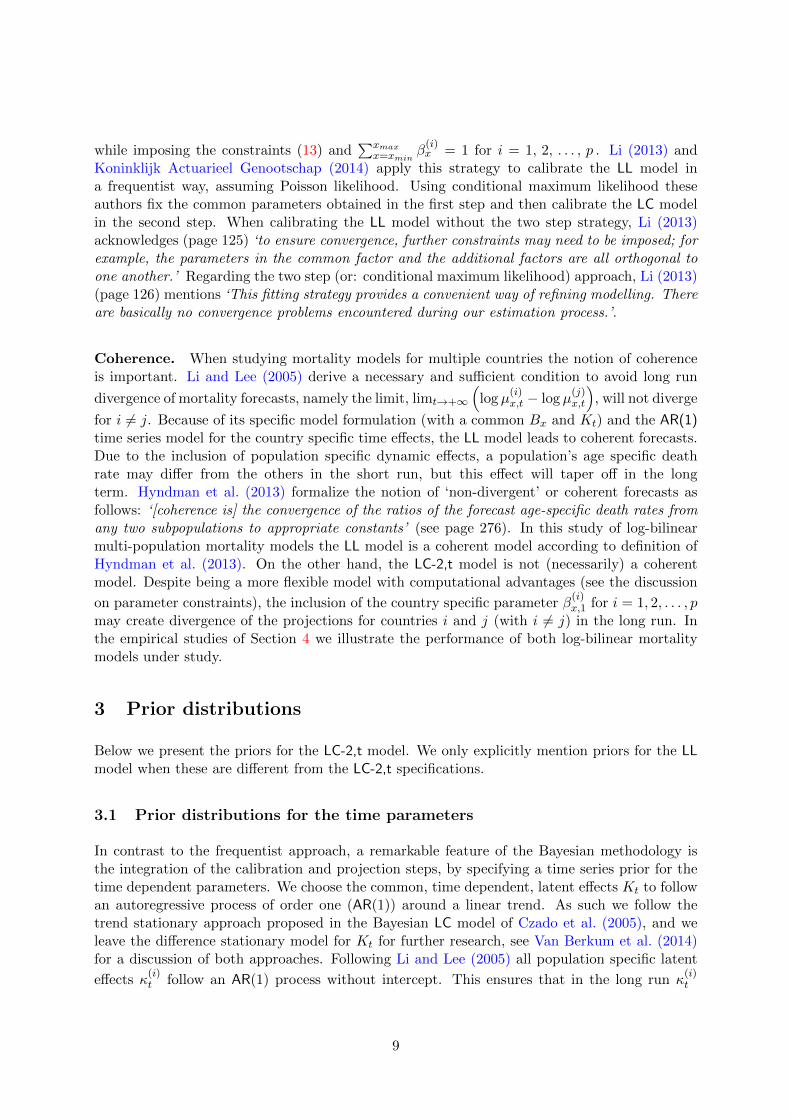
Estimates and credibility intervals in the LC-2,t model. Figure 1 shows the parameter
estimates of α(M)x , α
(F )x (top row), β
(M)x,1 , β
(F )x,1 (second row) and β
(M)x,2 and β
(F )x,2 (bottom row) as
well as their 95% credibility intervals. The Bayesian estimates of the αx parameters are verysimilar to the age specific intercepts estimated with a single population LC model. The Bayesian
estimates of β(M)x,1 and β
(F )x,1 have a similar course, though for ages around 25 and 75, β
(M)x,1 and
β(F )x,1 show some clear differences.
The samples from the posterior distribution of the common period effect Kt, displayed in theleft panel of Figure 2, show mean reversion around a linear, downward trend with the posteriormedian of ρ equal to 0.947. The intercept of the linear trend has posterior median equal to
48.83 and the posterior median of the slope is −1.583. The gender specific latent effects κ(F )t
and κ(M)t are in the right panel of Figure 2. These show mean reversion around 0 with the
posterior median of ρ(M) equal to 0.94 and the posterior median of ρ(F ) is 0.795. We compare
the Bayesian estimates of Kt to the trend obtained with MLE in the Poisson LC model on D(•)x,t
and E(•)x,t and with the common trend estimated using SVD in the LL model. The Bayesian
common trend in the LC-2,t model is very similar to, though visibly different from, these twobenchmark estimates.
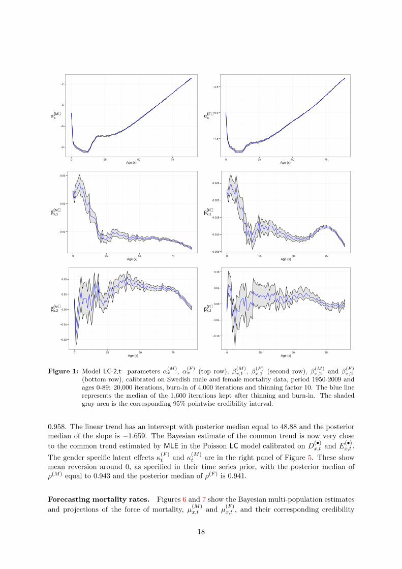
Estimates and credibility intervals in the LL model. Figure 3 shows the parameter
estimates and the 95% credibility intervals of α(M)x , α
(F )x , Ax and Figure 4 shows corresponding
results for β(M)x , β
(F )x , Bx in the Bayesian LL model. As expected, Ax and Bx capture the
common pattern in the age specific intercepts and slopes shown in Figure 1.
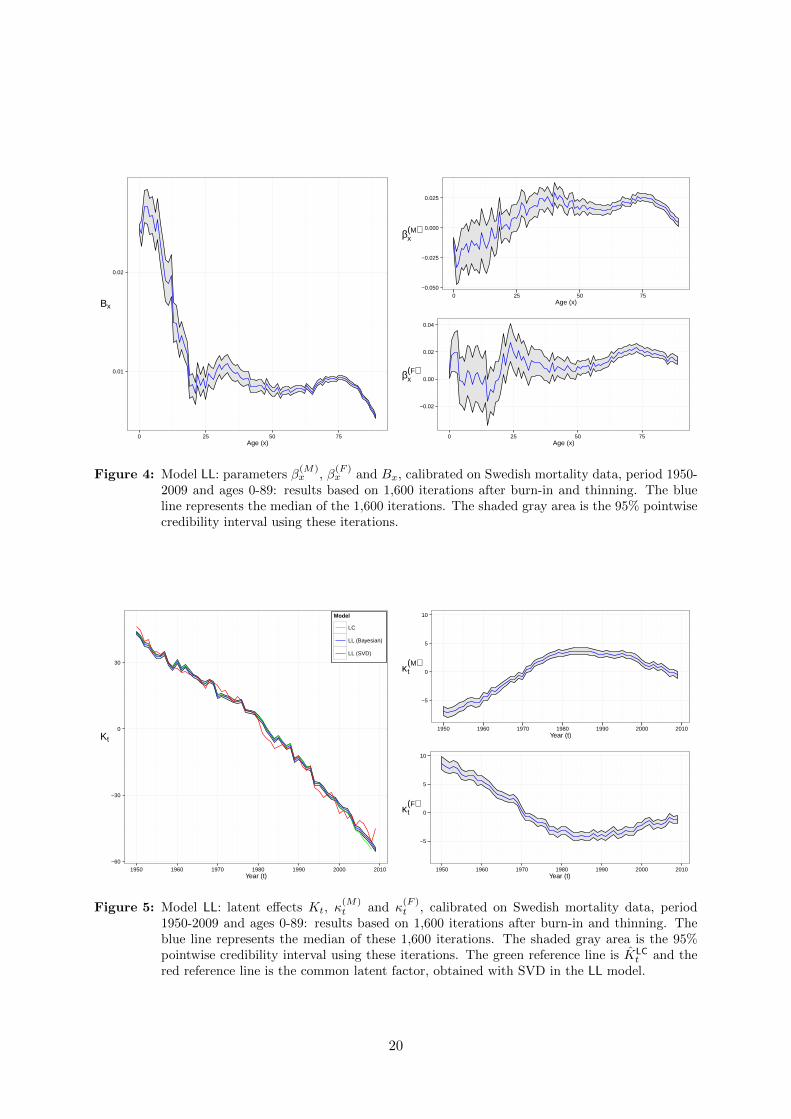
Estimates and credibility intervals of the common latent effect, Kt, and the gender specific
period effects, κ(F )t and κ
(M)t , are in Figure 5. The common trend shows a downward, rather
linear pattern, mean reverting around a linear trend with the posterior median of ρ equal to
17If σ2 ∼ IG(a, b) then E(σ2) = ba−1
and Var(σ2) = b2
(a−1)2(a−2).
18Trace plots of the (hyper)parameters used in the model are available in a note accompanying this paper,downloadable from www.econ.kuleuven.be/anastasios.bardoutsos.
17
−8
−6
−4
−2
0 25 50 75Age (x)
αx(M)
−7.5
−5.0
−2.5
0 25 50 75Age (x)
αx(F)
0.01
0.02
0.03
0 25 50 75Age (x)
βx,1(M)
0.005
0.010
0.015
0.020
0.025
0 25 50 75Age (x)
βx,1(F)
−0.02
−0.01
0.00
0.01
0.02
0 25 50 75Age (x)
βx,2(M)
−0.10
−0.05
0.00
0.05
0.10
0 25 50 75Age (x)
βx,2(F)
Figure 1: Model LC-2,t: parameters α(M)x , α
(F )x (top row), β
(M)x,1 , β
(F )x,1 (second row), β
(M)x,2 and β
(F )x,2
(bottom row), calibrated on Swedish male and female mortality data, period 1950-2009 andages 0-89: 20,000 iterations, burn-in of 4,000 iterations and thinning factor 10. The blue linerepresents the median of the 1,600 iterations kept after thinning and burn-in. The shadedgray area is the corresponding 95% pointwise credibility interval.
0.958. The linear trend has an intercept with posterior median equal to 48.88 and the posteriormedian of the slope is −1.659. The Bayesian estimate of the common trend is now very close
to the common trend estimated by MLE in the Poisson LC model calibrated on D(•)x,t and E
(•)x,t .
The gender specific latent effects κ(F )t and κ
(M)t are in the right panel of Figure 5. These show
mean reversion around 0, as specified in their time series prior, with the posterior median ofρ(M) equal to 0.943 and the posterior median of ρ(F ) is 0.941.
Forecasting mortality rates. Figures 6 and 7 show the Bayesian multi-population estimates
and projections of the force of mortality, µ(M)x,t and µ
(F )x,t , and their corresponding credibility
18

−60
−30
0
30
1950 1960 1970 1980 1990 2000 2010Year (t)
Kt
Model
LC
LC−2,t
LL (SVD)
−10
0
10
1950 1960 1970 1980 1990 2000 2010Year (t)
κt(M)
−10
0
10
1950 1960 1970 1980 1990 2000 2010Year (t)
κt(F)
Figure 2: Model LC-2,t: latent effects Kt, κ(M)t and κ
(F )t , calibrated on Swedish male and female mor-
tality data, period 1950-2009 and ages 0-89: 20,000 iterations, burn-in of 4,000 iterations andthinning factor 10. The blue line represents the median calculated from the 1,600 iterationskept after thinning and burn-in. The shaded gray area is the corresponding 95% pointwisecredibility interval. The green reference line is KLC
t and the red reference line is the commonlatent factor, obtained with SVD in the LL model.
−9
−7
−5
−3
0 25 50 75Age (x)
Ax
0.0
0.1
0.2
0.3
0.4
0 25 50 75Age (x)
αx(M)
−0.6
−0.4
−0.2
0 25 50 75Age (x)
αx(F)
Figure 3: Model LL: parameters α(M)x , α
(F )x and Ax, calibrated on Swedish mortality data, period 1950-
2009 and ages 0-89: results based on 1,600 iterations after burn-in and thinning. The blue linerepresents the median of these 1,600 iterations. The shaded gray area is the 95% pointwisecredibility interval using these iterations.
19
0.01
0.02
0 25 50 75Age (x)
Bx
−0.050
−0.025
0.000
0.025
0 25 50 75Age (x)
βx(M)
−0.02
0.00
0.02
0.04
0 25 50 75Age (x)
βx(F)
Figure 4: Model LL: parameters β(M)x , β
(F )x and Bx, calibrated on Swedish mortality data, period 1950-
2009 and ages 0-89: results based on 1,600 iterations after burn-in and thinning. The blueline represents the median of the 1,600 iterations. The shaded gray area is the 95% pointwisecredibility interval using these iterations.
−60
−30
0
30
1950 1960 1970 1980 1990 2000 2010Year (t)
Kt
Model
LC
LL (Bayesian)
LL (SVD)
−5
0
5
10
1950 1960 1970 1980 1990 2000 2010Year (t)
κt(M)
−5
0
5
10
1950 1960 1970 1980 1990 2000 2010Year (t)
κt(F)
Figure 5: Model LL: latent effects Kt, κ(M)t and κ
(F )t , calibrated on Swedish mortality data, period
1950-2009 and ages 0-89: results based on 1,600 iterations after burn-in and thinning. Theblue line represents the median of these 1,600 iterations. The shaded gray area is the 95%pointwise credibility interval using these iterations. The green reference line is KLC
t and thered reference line is the common latent factor, obtained with SVD in the LL model.
20

intervals for a selection of ages, namely the 20, 40, 60 and 80 years old. We benchmark theseresults against the estimates obtained with a Poisson MLE implementation of a gender specific LCmodel and the LL model calibrated using the Singular Value Decomposition. These benchmarkmodels use a random walk with drift for the period effect in the LC model and the common time
trend in the LL model, as well as an AR(1) model for the κ(i)t in the LL model. Parameters in
these time series models are estimated with MLE. The multi-population models reveal better insample fitting compared to the gender specific LC models, as illustrated by, for example, graph(b) in Figure 6. Both Bayesian multi-population models follow the observed data closely for allages in the sample, whereas the SVD calibration of LL for some ages is not capturing well theobserved evolution. Graphs (d) in Figure 6 and 7 illustrate this. Graph (b) in Figure 6 and (c)in Figure 7 illustrate that the LC-2,t model is following the observed data slightly more closelythan the LL model, due to the extra flexibility implied by using age and gender specific slopes
β(x,1i).
5.2 A set of European countries
Data. We select fourteen European countries, namely Austria, Belgium, Denmark, England-Wales, France, West Germany, Luxembourg, Netherlands, Switzerland, Finland, Iceland, Ire-land, Norway, and Sweden, and analyze mortality data for females as well as males from theHMD database. The Royal Dutch Actuarial Association19 uses this set of countries in its mostrecent stochastic projection model, see Koninklijk Actuarieel Genootschap (2014). This col-lection of countries meets the requirements formulated by Li and Lee (2005) for the study ofmortality rates as a group, i.e. they have similar socio-economic conditions and close connectionswhich are expected to continue in the future. We use ages from 0 until 89, as in Pitacco et al.(2009). Fitted values and forecasts for older ages can be obtained with a technique to close mor-tality tables, see for example Denuit and Goderniaux (2005) and Pitacco et al. (2009) (Section2.8). The calibration period in this illustration is the interval [1975, 2009], which is in line withthe optimal calibration period obtained for Belgian data in Pitacco et al. (2009) (Section 5.5.3)using the technique of Denuit and Goderniaux (2005). We choose the calibration period suchthat data for all countries in the considered group are available and the assumption of AR(1)around a linear trend is a reasonable assumption for the common latent effect. Results obtainedwith data on female mortality are discussed here; corresponding results for males are availablein the online appendix.
Initializing prior distributions. We initialize the priors as discussed in the example withSwedish data (see Section 5.1).
Estimates and credibility intervals in the LC-2,t model. Figure 8 shows the parameter
estimates for α(i)x in the LC-2,t model and corresponding credibility intervals. We present results
for Belgium, England-Wales and The Netherlands. These estimates are very close to the agespecific intercepts obtained with a single population, country specific LC model. The intervalsare narrow for all ages, similar to the findings of Czado et al. (2005).
Figures 9 and 10 show the estimates of β(i)x,1 and β
(i)x,2 and their corresponding credibility inter-
vals. For β(i)x,1 as well as β
(i)x,2 the estimates corresponding to ages in the range from 0 to 35
19See www.ag-ai.nl.
21

●●
●
●
●
●
●
●
●
●●●●
●●
●
●
●
●
●●●
●
●
●
●
●
●
●
●●
●
●
●
●
●
●
●
●
●
●●●
●●
●
●
●●
●
●●
●●
●
●●
●
●
●0.0005
0.0010
0.0015
1950 1975 2000 2025Year(t)
µx,t(M)
Model
LC
LC−2,t
LL (SVD)
●●
●
●
●
●
●
●
●
●●●●
●●
●
●
●
●
●●●
●
●
●
●
●
●
●
●●
●
●
●
●
●
●
●
●
●
●●●
●●
●
●
●●
●
●●
●●
●
●●
●
●
●0.0005
0.0010
0.0015
1950 1975 2000 2025Year(t)
µx,t(M)
Model
LC
LL (Bayesian)
LL (SVD)
(a) Death rate fan charts (µ(M)x,t ) for Swedish males, LC-2,t (left) and LL (right) at age 20.
●
●
●
●●
●
●
●
●
●
●
●
●●
●
●●
●
●
●
●●
●
●●●
●
●
●
●
●
●
●
●
●
●
●●●●
●
●
●
●
●
●
●
●●●
●
●●●●
●●
●
●●0.001
0.002
1950 1975 2000 2025Year(t)
µx,t(M)
●
●
●
●●
●
●
●
●
●
●
●
●●
●
●●
●
●
●
●●
●
●●●
●
●
●
●
●
●
●
●
●
●
●●●●
●
●
●
●
●
●
●
●●●
●
●●●●
●●
●
●●0.001
0.002
1950 1975 2000 2025Year(t)
µx,t(M)
(b) Death rate fan charts (µ(M)x,t ) for Swedish males, LC-2,t (left) and LL (right) at age 40.
●
●
●
●
●
●
●●●
●
●●●
●
●●●●
●●
●●
●●
●
●
●
●●
●
●
●●●
●
●●●
●●
●●●●●
●●●
●●●
●
●
●●●●
●●
●
0.005
0.010
0.015
1950 1975 2000 2025Year(t)
µx,t(M)
●
●
●
●
●
●
●●●
●
●●●
●
●●●●
●●
●●
●●
●
●
●
●●
●
●
●●●
●
●●●
●●
●●●●●
●●●
●●●
●
●
●●●●
●●
●
0.005
0.010
0.015
1950 1975 2000 2025Year(t)
µx,t(M)
(c) Death rate fan charts (µ(M)x,t ) for Swedish females, LC-2,t (left) and LL (right) at age 60.
●
●
●
●●
●●●
●●
●
●
●●●●●
●
●●
●
●
●
●●●
●●●●●
●●
●●●
●●
●
●●
●●●
●●●●
●●●●●
●●●
●●●●
0.05
0.10
1950 1975 2000 2025Year(t)
µx,t(M)
●
●
●
●●
●●●
●●
●
●
●●●●●
●
●●
●
●
●
●●●
●●●●●
●●
●●●
●●
●
●●
●●●
●●●●
●●●●●
●●●
●●●●
0.05
0.10
1950 1975 2000 2025Year(t)
µx,t(M)
(d) Death rate fan charts (µ(M)x,t ) for Swedish males, LC-2,t (left) and LL (right) at age 80.
Figure 6: Death rate fan charts for Swedish males at age 20, 40, 60 and 80 for the LC,2-t (left) and LL(right) models. 22

●
●
●
●
●●
●
●●●
●●●●●●
●
●
●
●●
●
●●
●
●
●●
●●●
●●
●●●●●●
●
●
●●●
●
●
●●●●
●●
●
●●
●●●●●
0.0005
0.0010
0.0015
1950 1975 2000 2025Year(t)
µx,t(F)
Model
LC
LC−2,t
LL (SVD)
●
●
●
●
●●
●
●●●
●●●●●●
●
●
●
●●
●
●●
●
●
●●
●●●
●●
●●●●●●
●
●
●●●
●
●
●●●●
●●
●
●●
●●●●●
0.0005
0.0010
0.0015
1950 1975 2000 2025Year(t)
µx,t(F)
Model
LC
LL (Bayesian)
LL (SVD)
(a) Death rate fan charts (µ(F )x,t ) for Swedish males, LC-2,t (left) and LL (right) at age 20.
●
●
●●
●●
●
●
●●
●
●●
●
●
●
●●●
●
●
●●
●
●
●●
●
●
●
●
●
●●●
●
●●
●●
●
●●●
●
●
●●
●●
●
●
●
●
●
●●●●
●
0.001
0.002
1950 1975 2000 2025Year(t)
µx,t(F)
●
●
●●
●●
●
●
●●
●
●●
●
●
●
●●●
●
●
●●
●
●
●●
●
●
●
●
●
●●●
●
●●
●●
●
●●●
●
●
●●
●●
●
●
●
●
●
●●●●
●
0.001
0.002
1950 1975 2000 2025Year(t)
µx,t(F)
(b) Death rate fan charts (µ(F )x,t ) for Swedish males, LC-2,t (left) and LL (right) at age 40.
●●
●●●●
●
●
●
●
●
●●
●
●
●●
●●
●●
●●
●
●●
●●●●
●●●
●●●
●●
●
●●
●●●
●●●●
●●
●
●●●
●●●
●●●0.005
0.010
0.015
1950 1975 2000 2025Year(t)
µx,t(F)
●●
●●●●
●
●
●
●
●
●●
●
●
●●
●●
●●
●●
●
●●
●●●●
●●●
●●●
●●
●
●●
●●●
●●●●
●●
●
●●●
●●●
●●●0.005
0.010
0.015
1950 1975 2000 2025Year(t)
µx,t(F)
(c) Death rate fan charts (µ(F )x,t ) for Swedish females, LC-2,t (left) and LL (right) at age 80.
●
●
●●
●●●
●●
●
●●
●
●●
●●●
●
●●
●●
●●●●
●
●●●
●●●●●●●●
●
●●
●●
●●●●●●●●●
●●●
●
●
●●
0.05
0.10
1950 1975 2000 2025Year(t)
µx,t(F)
●
●
●●
●●●
●●
●
●●
●
●●
●●●
●
●●
●●
●●●●
●
●●●
●●●●●●●●
●
●●
●●
●●●●●●●●●
●●●
●
●
●●
0.05
0.10
1950 1975 2000 2025Year(t)
µx,t(F)
(d) Death rate fan charts (µ(F )x,t ) for Swedish females, LC-2,t (left) and LL (right) at age 80.
Figure 7: Death rate fan charts for Swedish females at age 20, 40, 60 and 80 for the LC,2-t (left) andLL (right) models. 23

−7.5
−5.0
−2.5
0 25 50 75Age (x)
αx(BE)
−8
−6
−4
−2
0 25 50 75Age (x)
αx(EW)
−8
−6
−4
−2
0 25 50 75Age (x)
αx(NL)
Figure 8: Model LC-2,t: parameter α(i)x for Belgium, England-Wales and The Netherlands: female data,
period 1975-2009 and ages 0-89. 20,000 iterations, burn-in of 4,000 iterations and thinningfactor 10. The blue line represents the median of the 1,600 iterations kept after thinning andburn-in. The shaded gray area is the 95% pointwise credibility interval using these iterations.
(approximately) show the largest uncertainty. Estimates corresponding to different countriesshow similarities, though differences are clearly visible.
0.01
0.02
0.03
0 25 50 75Age (x)
βx,1(BE)
0.005
0.010
0.015
0.020
0 25 50 75Age (x)
βx,1(EW)
0.01
0.02
0 25 50 75Age (x)
βx,1(NL)
Figure 9: Model LC-2,t: parameter β(i)x,1 for Belgium, England-Wales and The Netherlands: female data,
period 1975-2009 and ages 0-89. 20,000 iterations, burn-in of 4,000 iterations and thinningfactor 10. The blue line represents the median of the 1,600 iterations kept after thinning andburn-in. The shaded gray area is the 95% pointwise credibility interval using these iterations.
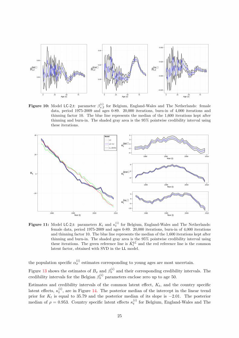
Estimates and credibility intervals for the common latent effect, Kt, and the country specific
latent effects, κ(i)t , are in Figure 11. Again we add the time trend of a LC model on D
(•)x,t and E
(•)x,t ,
as well as the common trend obtained with SVD in the LL model, as reference lines. The posteriormedian of the intercept used in the linear trend prior of Kt is equal to 35.72 and the posterior
median of the slope is−1.81. The posterior median of ρ is 0.96. Country specific latent effects κ(i)t
are shown in the right panel of Figure 11 for a selection of countries (namely Belgium, England-Wales and The Netherlands). These country specific effects show mean reversion around 0, asspecified in their time series prior, with posterior median of ρ(BE) = 0.819, ρ(EW) = 0.876 and
ρ(NL) = 0.832. The uncertainty in the κ(i)t estimates of Belgium and the Netherlands is larger
than the corresponding uncertainty for England-Wales.
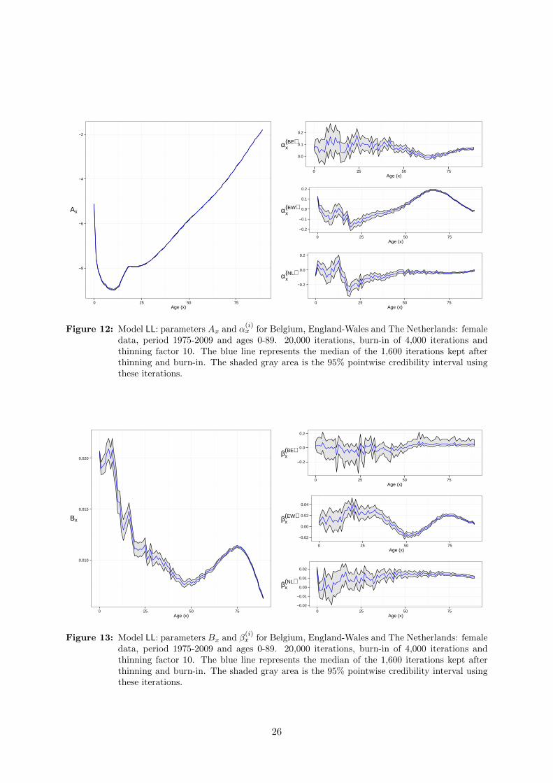
Estimates and credibility intervals in the LL model. Figure 12 shows the parameter
estimates of Ax, α(i)x and their corresponding credibility intervals. According to the intervals for
24
0.00
0.05
0 25 50 75Age (x)
βx,2(BE)
0.00
0.02
0.04
0 25 50 75Age (x)
βx,2(EW)
−0.025
0.000
0.025
0.050
0 25 50 75Age (x)
βx,2(NL)
Figure 10: Model LC-2,t: parameter β(i)x,2 for Belgium, England-Wales and The Netherlands: female
data, period 1975-2009 and ages 0-89. 20,000 iterations, burn-in of 4,000 iterations andthinning factor 10. The blue line represents the median of the 1,600 iterations kept afterthinning and burn-in. The shaded gray area is the 95% pointwise credibility interval usingthese iterations.
−20
0
20
40
1980 1990 2000 2010Year (t)
Kt
Model
LC
LC−2,t
LL (SVD)
−6
−3
0
3
6
1980 1990 2000 2010Year (t)
κt(BE)
−5
0
5
1980 1990 2000 2010Year (t)
κt(EW)
−10
−5
0
5
1980 1990 2000 2010Year (t)
κt(NL)
Figure 11: Model LC-2,t: parameters Kt and κ(i)t for Belgium, England-Wales and The Netherlands:
female data, period 1975-2009 and ages 0-89. 20,000 iterations, burn-in of 4,000 iterationsand thinning factor 10. The blue line represents the median of the 1,600 iterations kept afterthinning and burn-in. The shaded gray area is the 95% pointwise credibility interval usingthese iterations. The green reference line is KLC
t and the red reference line is the commonlatent factor, obtained with SVD in the LL model.
the population specific α(i)x estimates corresponding to young ages are most uncertain.
Figure 13 shows the estimates of Bx and β(i)x and their corresponding credibility intervals. The
credibility intervals for the Belgian β(i)x parameters enclose zero up to age 50.
Estimates and credibility intervals of the common latent effect, Kt, and the country specific
latent effects, κ(i)t , are in Figure 14. The posterior median of the intercept in the linear trend
prior for Kt is equal to 35.79 and the posterior median of its slope is −2.01. The posterior
median of ρ = 0.953. Country specific latent effects κ(i)t for Belgium, England-Wales and The
25
−8
−6
−4
−2
0 25 50 75Age (x)
Ax
0.0
0.1
0.2
0 25 50 75Age (x)
αx(BE)
−0.2
−0.1
0.0
0.1
0.2
0 25 50 75Age (x)
αx(EW)
−0.2
0.0
0.2
0 25 50 75Age (x)
αx(NL)
Figure 12: Model LL: parameters Ax and α(i)x for Belgium, England-Wales and The Netherlands: female
data, period 1975-2009 and ages 0-89. 20,000 iterations, burn-in of 4,000 iterations andthinning factor 10. The blue line represents the median of the 1,600 iterations kept afterthinning and burn-in. The shaded gray area is the 95% pointwise credibility interval usingthese iterations.
0.010
0.015
0.020
0 25 50 75Age (x)
Bx
−0.2
0.0
0.2
0 25 50 75Age (x)
βx(BE)
−0.02
0.00
0.02
0.04
0 25 50 75Age (x)
βx(EW)
−0.02
−0.01
0.00
0.01
0.02
0 25 50 75Age (x)
βx(NL)
Figure 13: Model LL: parameters Bx and β(i)x for Belgium, England-Wales and The Netherlands: female
data, period 1975-2009 and ages 0-89. 20,000 iterations, burn-in of 4,000 iterations andthinning factor 10. The blue line represents the median of the 1,600 iterations kept afterthinning and burn-in. The shaded gray area is the 95% pointwise credibility interval usingthese iterations.
26

Netherlands are shown in the right panel of Figure 11. These country specific effects have a
posterior median of ρ(BE) = 0.758, ρ(EW) = 0.878 and ρ(NL) = 0.919. The uncertainty of κ(i)t for
Belgium and The Netherlands is larger than the corresponding uncertainty for England-Wales.
−20
0
20
40
1980 1990 2000 2010Year (t)
Kt
Model
LC
LL (Bayesian)
LL (SVD)
−1
0
1
2
1980 1990 2000 2010Year (t)
κt(BE)
−7.5
−5.0
−2.5
0.0
2.5
1980 1990 2000 2010Year (t)
κt(EW)
−10
−5
0
5
10
1980 1990 2000 2010Year (t)
κt(NL)
Figure 14: Model LL: parameters Kt and κ(i)t for Belgium, England-Wales and The Netherlands: female
data, period 1975-2009 and ages 0-89. 20,000 iterations, burn-in of 4,000 iterations andthinning factor 10. The blue line represents the median of the 1,600 iterations kept afterthinning and burn-in. The shaded gray area is the 95% pointwise credibility interval usingthese iterations. The green reference line is KLC
t and the red reference line is the commonlatent factor, obtained with SVD in the LL model.
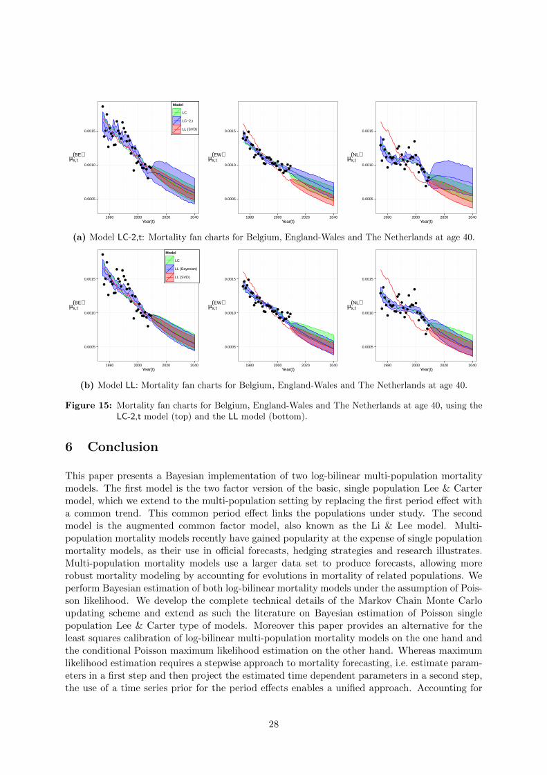
Forecasting mortality: Belgium, England-Wales, The Netherlands. Figures 15 and
16 show calibrated death rates, µ(i)x,t, their corresponding credibility intervals and forecasts for a
selection of ages, namely the 40 and 60 years old for both Bayesian multi-population models. Asin Section 5.1 we benchmark these results against the estimates obtained with a Poisson MLEimplementation of a country specific LC model and the LL model calibrated using the SingularValue Decomposition. Both Bayesian multi-population models follow the observed data closelyfor all ages in the sample, whereas the SVD calibration of LL for some ages is not capturingwell the observed evolution. This is clearly illustrated by the graphs of England-Wales andThe Netherlands. The age 40 forecasts for Belgium and The Netherlands as obtained with theLC-2,t model are much more uncertain than the corresponding forecasts for England-Wales onthe one hand and the forecasts obtained with the LL model on the other hand. The increase inuncertainty is due to the larger estimate and uncertainty of β
(i)x,1 and β
(i)x,2 in Figures 9 and 10.
Forecasting mortality: Austria versus West-Germany. A comparison between the deathrate estimates and forecasts of a very large country, i.e. West-Germany, and a very small country,i.e. Austria, illustrates how uncertainty is reflected by the Bayesian multi-population models inthe study. For a selection of ages Figure 17 and Figure 18 show the estimated and forecastedforces of mortality for Austria (top row) and West-Germany (bottom row). The results for Aus-tria, with a population of approximately 8 million inhabitants, clearly reflect more uncertaintythan the corresponding results for West-Germany.
27
●
●
●
●
●
●
●●
●●
●
●●
●
●
●●
●
●
●
●
●
●
●
●●
●
●●●
●
●
●
●●
0.0005
0.0010
0.0015
1980 2000 2020 2040Year(t)
µx,t(BE)
Model
LC
LC−2,t
LL (SVD)
●
●
●●
●
●
●●
●●
●
●
●
●●
●●
●●●●
●●●●
●
●●
●
●●●
●
●●
0.0005
0.0010
0.0015
1980 2000 2020 2040Year(t)
µx,t(EW)
●
●
●
●
●
●
●●●●
●●
●●
●
●
●
●
●●
●
●●●
●
●
●
●
●
●●●
●
●●
0.0005
0.0010
0.0015
1980 2000 2020 2040Year(t)
µx,t(NL)
(a) Model LC-2,t: Mortality fan charts for Belgium, England-Wales and The Netherlands at age 40.
●
●
●
●
●
●
●●
●●
●
●●
●
●
●●
●
●
●
●
●
●
●
●●
●
●●●
●
●
●
●●
0.0005
0.0010
0.0015
1980 2000 2020 2040Year(t)
µx,t(BE)
Model
LC
LL (Bayesian)
LL (SVD)
●
●
●●
●
●
●●
●●
●
●
●
●●
●●
●●●●
●●●●
●
●●
●
●●●
●
●●
0.0005
0.0010
0.0015
1980 2000 2020 2040Year(t)
µx,t(EW)
●
●
●
●
●
●
●●●●
●●
●●
●
●
●
●
●●
●
●●●
●
●
●
●
●
●●●
●
●●
0.0005
0.0010
0.0015
1980 2000 2020 2040Year(t)
µx,t(NL)
(b) Model LL: Mortality fan charts for Belgium, England-Wales and The Netherlands at age 40.
Figure 15: Mortality fan charts for Belgium, England-Wales and The Netherlands at age 40, using theLC-2,t model (top) and the LL model (bottom).
6 Conclusion
This paper presents a Bayesian implementation of two log-bilinear multi-population mortalitymodels. The first model is the two factor version of the basic, single population Lee & Cartermodel, which we extend to the multi-population setting by replacing the first period effect witha common trend. This common period effect links the populations under study. The secondmodel is the augmented common factor model, also known as the Li & Lee model. Multi-population mortality models recently have gained popularity at the expense of single populationmortality models, as their use in official forecasts, hedging strategies and research illustrates.Multi-population mortality models use a larger data set to produce forecasts, allowing morerobust mortality modeling by accounting for evolutions in mortality of related populations. Weperform Bayesian estimation of both log-bilinear mortality models under the assumption of Pois-son likelihood. We develop the complete technical details of the Markov Chain Monte Carloupdating scheme and extend as such the literature on Bayesian estimation of Poisson singlepopulation Lee & Carter type of models. Moreover this paper provides an alternative for theleast squares calibration of log-bilinear multi-population mortality models on the one hand andthe conditional Poisson maximum likelihood estimation on the other hand. Whereas maximumlikelihood estimation requires a stepwise approach to mortality forecasting, i.e. estimate param-eters in a first step and then project the estimated time dependent parameters in a second step,the use of a time series prior for the period effects enables a unified approach. Accounting for
28

●
●●
●
●
●
●●●
●
●●
●●●
●
●
●
●●●●
●●
●●●●
●●●
●
●
●●
0.003
0.006
0.009
1980 2000 2020 2040Year(t)
µx,t(BE)
Model
LC
LC−2,t
LL (SVD)
●●●●●
●
●●●●●
●●
●●●●
●●
●●●●●●
●
●●●●
●●
●●●
0.003
0.006
0.009
1980 2000 2020 2040Year(t)
µx,t(EW)
●
●
●
●●●
●
●
●
●●●
●
●●●●●
●
●●
●●
●
●
●●●●
●
●
●●●
●
0.003
0.006
0.009
1980 2000 2020 2040Year(t)
µx,t(NL)
(a) Model LC-2,t: Mortality fan charts for Belgium, England-Wales and The Netherlands at age 60.
●
●●
●
●
●
●●●
●
●●
●●●
●
●
●
●●●●
●●
●●●●
●●●
●
●
●●
0.003
0.006
0.009
1980 2000 2020 2040Year(t)
µx,t(BE)
Model
LC
LL (Bayesian)
LL (SVD)
●●●●●
●
●●●●●
●●
●●●●
●●
●●●●●●
●
●●●●
●●
●●●
0.003
0.006
0.009
1980 2000 2020 2040Year(t)
µx,t(EW)
●
●
●
●●●
●
●
●
●●●
●
●●●●●
●
●●
●●
●
●
●●●●
●
●
●●●
●
0.003
0.006
0.009
1980 2000 2020 2040Year(t)
µx,t(NL)
(b) Model LL: Mortality fan charts for Belgium, England-Wales and The Netherlands at age 60.
Figure 16: Mortality fan charts for Belgium, England-Wales and The Netherlands at age 60, using theLC-2,t model (top) and the LL model (bottom).
all sources of uncertainty is another direct advantage of the Bayesian approach and allows topresent parameter estimates as well as their corresponding uncertainty. We demonstrate the useof the Bayesian log-bilinear multi-population models with two empirical studies, the analysisof Swedish male and female mortality during 1950-2009 and the analysis of a collection of 14European countries during 1975-2009. The calibrated Poisson multi-population models followthe observed data closely, whereas the least squares estimation of the augmented common factormodel for some calibration periods and specific ages does not capture well the observed mor-tality data. In future work we plan on developing the technicalities involved in the Bayesianestimation of other multi-population models. The extension of the present work to the jointmodeling of portfolio and population mortality data is another direction for future research.
29
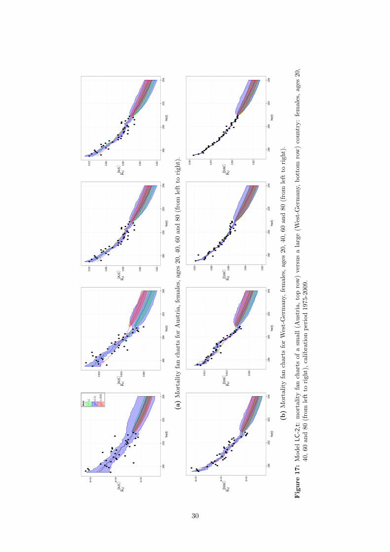
●
●
●●
●●
●
●
●
●
●
●●
●
●
●
●
●
●
●
●●
●
●
●●
●●
●
●●
●
●
●●
2e−0
4
4e−0
4
6e−0
4
1980
2000
2020
2040
Year
(t)
µ x,t(AUS)
Mode
l LC LC−2
,t
LL (S
VD)
●
●
●
●
●●
●●
●
●
●
●
●
●
●
●
●
●
●
●
●
●
●
●
●
●
●
●
●
●
●●
●
●
●0.
0005
0.00
10
0.00
15
1980
2000
2020
2040
Year
(t)
µ x,t(AUS)
●
●
●
●●
●
●●
●●
●
●
●
●
●●
●
●
●
●
●●
●
●●
●●
●
●●
●
●
●
●
●
0.00
2
0.00
4
0.00
6
0.00
8
0.01
0
1980
2000
2020
2040
Year
(t)
µ x,t(AUS)
●
●
●
●●
●
●●
●●
●
●
●
●
●●
●
●
●
●
●●
●
●●
●●
●
●●
●
●
●
●
●
0.00
2
0.00
4
0.00
6
0.00
8
0.01
0
1980
2000
2020
2040
Year
(t)
µ x,t(AUS)
(a)
Mor
tali
tyfa
nch
arts
for
Aust
ria,
fem
ale
s,ages
20,
40,
60
an
d80
(fro
mle
ftto
right)
.
●●
●
●
●
●●
●●
●
●●
●
●
●●
●●
●
●
●●
●
●
●
●●
●●
●
●
●●
●●
2e−0
4
4e−0
4
6e−0
4
1980
2000
2020
2040
Year
(t)
µ x,t(DUW
)
●
●
●●
●●
●
●●
●●
●
●●
●●
●●
●●
●●
●●
●
●●
●
●●
●●
●●
●
0.00
05
0.00
10
0.00
15
1980
2000
2020
2040
Year
(t)
µ x,t(DUW
)
●
●●
●
●
●
●●
●
●●
●
●●
●●
●
●●
●●
●●
●●
●
●
●
●●
●
●
●●
●
0.00
2
0.00
4
0.00
6
0.00
8
0.01
0
1980
2000
2020
2040
Year
(t)
µ x,t(DUW
)
●
●
●●
●●
●●
●
●●
●
●●
●●
●●
●●
●
●●
●
●
●
●●
●
●●
●●
●●
0.02
5
0.05
0
0.07
5
0.10
0
1980
2000
2020
2040
Year
(t)
µ x,t(DUW
)
(b)
Mor
tali
tyfa
nch
arts
for
Wes
t-G
erm
any,
fem
ale
s,ages
20,
40,
60
an
d80
(fro
mle
ftto
right)
.
Fig
ure
17:
Mod
elLC-2,t
:m
orta
lity
fan
char
tsof
asm
all
(Au
stri
a,
top
row
)ve
rsu
sa
larg
e(W
est-
Ger
many,
bott
om
row
)co
untr
y:
fem
ale
s,ages
20,
40,
60an
d80
(fro
mle
ftto
righ
t),
cali
bra
tion
per
iod
1975-2
009.
30

●
●
●●
●●
●
●
●
●
●
●●
●
●
●
●
●
●
●
●●
●
●
●●
●●
●
●●
●
●
●●
2e−0
4
4e−0
4
6e−0
4
1980
2000
2020
2040
Year
(t)
µ x,t(AUS)
Mode
l LC LL (B
ayes
ian)
LL (S
VD)
●
●
●
●
●●
●●
●
●
●
●
●
●
●
●
●
●
●
●
●
●
●
●
●
●
●
●
●
●
●●
●
●
●0.
0005
0.00
10
0.00
15
1980
2000
2020
2040
Year
(t)
µ x,t(AUS)
●
●
●
●●
●
●●
●●
●
●
●
●
●●
●
●
●
●
●●
●
●●
●●
●
●●
●
●
●
●
●
0.00
2
0.00
4
0.00
6
0.00
8
0.01
0
1980
2000
2020
2040
Year
(t)
µ x,t(AUS)
●
●
●
●●
●
●●
●●
●
●
●
●
●●
●
●
●
●
●●
●
●●
●●
●
●●
●
●
●
●
●
0.00
2
0.00
4
0.00
6
0.00
8
0.01
0
1980
2000
2020
2040
Year
(t)
µ x,t(AUS)
(a)
Mor
tali
tyfa
nch
arts
for
Aust
ria,
fem
ale
s,ages
20,
40,
60
an
d80
(fro
mle
ftto
right)
.
●●
●
●
●
●●
●●
●
●●
●
●
●●
●●
●
●
●●
●
●
●
●●
●●
●
●
●●
●●
2e−0
4
4e−0
4
6e−0
4
1980
2000
2020
2040
Year
(t)
µ x,t(DUW
)
●
●
●●
●●
●
●●
●●
●
●●
●●
●●
●●
●●
●●
●
●●
●
●●
●●
●●
●
0.00
05
0.00
10
0.00
15
1980
2000
2020
2040
Year
(t)
µ x,t(DUW
)
●
●●
●
●
●
●●
●
●●
●
●●
●●
●
●●
●●
●●
●●
●
●
●
●●
●
●
●●
●
0.00
2
0.00
4
0.00
6
0.00
8
0.01
0
1980
2000
2020
2040
Year
(t)
µ x,t(DUW
)
●
●
●●
●●
●●
●
●●
●
●●
●●
●●
●●
●
●●
●
●
●
●●
●
●●
●●
●●
0.02
5
0.05
0
0.07
5
0.10
0
1980
2000
2020
2040
Year
(t)
µ x,t(DUW
)
(b)
Mor
tali
tyfa
nch
arts
for
Wes
t-G
erm
any,
fem
ale
s,ages
20,
40,
60
an
d80
(fro
mle
ftto
right)
.
Fig
ure
18:
Mod
elLL:
mor
tali
tyfa
nch
arts
ofa
smal
l(A
ust
ria,
top
row
)ve
rsu
sa
larg
e(W
est-
Ger
many,
bott
om
row
)co
untr
y:
fem
ale
s,ages
20,
40,
60
and
80(f
rom
left
tori
ght)
,ca
lib
rati
onp
erio
d1975-2
009.
31

A Metropolis-Hastings algorithm
A.1 Algorithm for Kt and κ(i)t
We use Metropolis-Hastings to update Kt. Assume that we have K[l]s for all s < t at iteration
[l]. Then we proceed as follows:
1. Generate a candidate K∗t from a normal distribution with mean K[l]t and variance s2Kt
.We start with s2Kt
= 1 and we update this value every 100 simulations to ensure that theacceptance probability is in the interval [20%, 50%]. For more details see Czado et al.(2005).
2. We use (37) and (38) to calculate the acceptance probability as follows:
ψ(K[l]t ,K
∗t ) = min
1,f(K∗t
∣∣∣K [l]−t,κ,α,β1,β2,D, σ
2K , ρ,γ
)f(K
[l]t
∣∣∣K [l]−t,κ,α,β1,β2,D, σ
2K , ρ,γ
) (47)
3. Generate a realization u from the Uniform(0, 1) distribution. If u ≤ ψ(K[l]t ,K
∗t ) we accept
the candidate, i.e. K[l+1]t = K∗t . If u > ψ(K
[l]t ,K
∗t ) we reject the candidate, so K
[l+1]t =
K[l]t .
4. Apply the constraint∑tmax
t=tminKt = 0.
The MH steps are similar for the parameters κ(i)t .
A.2 Algorithm for β(i)x,1 and β
(i)x,2
Assume that we have β(i)[l]x,1 at iteration [l]. The Metropolis-Hastings updating scheme for β
(i)x,1
goes as follows:
1. Generate a candidate β(i)∗x,1 from a truncated normal distribution in the interval (−1, 1)
with mean β(i)[l]x,1 and variance equal to s2β1
= 1. The choice of the interval stems from
empirical results. We start with variance s2β1and we update every 100 simulations to
ensure that the acceptance probability is in the interval [20%, 50%]. For more details seeCzado et al. (2005).
2. Calculate the acceptance probability as follows,
ψ(β(i)[l]x,1 , β
(i)∗x,1
)= min
1,f(β(i)∗x,1 |β
(i)[l]−x,1,α,κ,K, σ2β1
)f(β(i)[l]x,1 |β
(i)[l]−x,1,α,κ,K, σ2β1
) (48)
3. Generate a realization u from the Uniform(0, 1) distribution. If u ≤ ψ(β(i)[l]x,1 , β
(i)∗x,1
)we
accept the candidate, i.e. β(i)[l+1]x,1 = β
(i)∗x,1 . If u > ψ
(β(i)[l]x,1 , β
(i)∗x,1
)we reject the candidate,
so β(i)[l+1]x,1 = β
(i)[l]x,1 .
32

4. Apply constraint1
p
∑pi=1
∑xmaxx=xmin
β(i)x,1 = 1.
The MH steps are similar for the parameters β(i)x,2.
A.3 Algorithm for ρ and ρ(i)
Assume ρ[l] at iteration [l] is available, then the MH updating scheme for ρ goes as follows.
1. Generate a candidate logit (ρ∗) from a normal distribution with mean logit(ρ[l])
and vari-ance s2ρ = 0.252. This distribution is no longer symmetric. We start with variance s2ρand we update every 100 simulations to ensure that the acceptance probability is in theinterval [20%, 50%]. For more details see Czado et al. (2005).
2. Calculate the acceptance probability as follows
ψ(ρ[l], ρ∗) = min
1,f(ρ∗∣∣∣K,γ, σ2K
)f(ρ[l]∣∣∣K,γ, σ2K
) g (ρ[l]|ρ∗)g(ρ∗|ρ[l]
) , (49)
where g is the proposal distribution, namely the logit normal distribution and
g(ρ[l]|ρ∗
)g(ρ∗|ρ[l]
) =ρ[l](1− ρ[l]
)ρ∗ (1− ρ∗)
.
3. Generate a realization u from the Uniform(0, 1) distribution. If u ≤ ψ(ρ[l], ρ∗) we acceptthe candidate, ρ[l+1] = ρ∗. If u > ψ(ρ[l], ρ∗) we reject the candidate, so ρ[l+1] = ρ[l].
The MH steps are similar for the hyperparameters ρ(i).
References
Abel, G., Bijak, J., Forster, J., Raymer, J., and Smith, P. (2010). What do Bayesianmethods offer population forecasters? ESRC Centre for Population Change, Working Pa-per, 6: http: // www. cpc. ac. uk/ publications/ cpc_ working_ papers/ pdf/ 2010_ WP6_
What_ do_ Bayesian_ Methods_ Offer_ Population_ Forecasters_ Abel_ et_ al. pdf .
Barrieu, P., Bensusan, H., Karoui, N. E., Hillairet, C., Loisel, S., Ravanelli, C., and Salhi,Y. (2012). Understanding, modelling and managing longevity risk : key issues and mainchallenges. Scandinavian Actuarial Journal, 3:203–231.
Bray, I. (2002). Application of Markov Chain Monte Carlo methods to projecting cancer inci-dence and mortality. Applied Statistics, 3:3–43.
Brouhns, N., Denuit, M., and Vermunt, J. (2002). A Poisson log-bilinear regression approach tothe construction of projected life tables. Insurance: Mathematics and Economics, 31:373–393.
Cairns, A., Blake, D., and Dowd, K. (2006). A two-factor model for stochastic mortality withparameter uncertainty: theory and calibration. Journal of Risk and Insurance, 73:687–718.
33
Cairns, A., Blake, D., Dowd, K., Coughlan, G., Epstein, D., Ong, A., and Balevich, I. (2009). Aquantitative comparison of stochastic mortality models using data from England and Walesand the United States. North American Actuarial Journal, 13(1):1–35.
Cairns, A., Blake, D., Dowd, K., Coughlan, G., and Khalaf-Allah, M. (2011). Bayesian stochasticmortality modelling for two populations. ASTIN Bulletin, 41:29–59.
Carter, L. and Lee, R. (1992). Forecasting demographic components: modeling and forecastingUS sex differentials in mortality. International Journal of Forecasting, 8:393–411.
Congdon, P. (2006). Bayesian Statistical Modelling. Wiley, England.
Czado, C., Delwarde, A., and Denuit, M. (2005). Bayesian Poisson log–bilinear mortality pro-jections. Insurance: Mathematics and Economics, 36:260–284.
Danesi, I. (2014). Forecasting Mortality in Related Populations Using Lee-Carter Type Models.PhD thesis, Universita degli Studi di Padova. http://paduaresearch.cab.unipd.it/6736/.
De Waegenaere, A., Hong, L., and Melenberg, B. (2013). The choice of sample size for mor-tality forecasting: A Bayesian approach. Working Paper: http://www.netspar.nl/files/
Evenementen/2013-11-08%20PD/005%20hong%20li.pdf.
Dellaportas, P., Smith, A., and Stavropoulos, P. (2001). Bayesian analysis of mortality data.Journal of the Royal Statistical Society: Series A (Statistics in Society), 164(2):275–291.
Denuit, M. and Goderniaux, A.-C. (2005). Closing and projecting life tables using log-linearmodels. Bulletin of the Swiss Association of Actuaries, 1:29–48.
Dowd, K., Blake, D., Cairns, A., Coughlan, G., and Khalaf-Allah, M. (2011). A gravity model ofmortality rates for two related populations. North American Actuarial Journal, 15:334–356.
Fushimi, T. and Kogure, A. (2014). A Bayesian approach to longevity derivative pric-ing under stochastic interest rates with a two-factor Lee-Carter model. ARIA 2014 An-nual Meeting: http: // www. aria. org/ Annual_ Meeting/ 2014/ 2014_ Accepted_ Papers/
4C/ Fushimi% 20and% 20Kogure. pdf .
Gelman, A., Carlin, J., Stern, H., Dunson, D., Vehtari, A., and Rubin, D. (2013). Bayesian dataanalysis. Chapman & Hall/CRC Texts in Statistical Science, New York.
Girosi, F. and King, G. (2008). Demographic Forecasting. Princeton: Princeton UniversityPress.
Haberman, S. and Renshaw, A. (2011). A comparative study of parametric mortality models.Insurance: Mathematics and Economics, 48:35–55.
Hatzopoulos, P. and Haberman, S. (2013). Common mortality modeling and coherent forecasts.an empirical analysis of worldwide mortality data. Insurance: Mathematics and Economics,52:320–337.
Hyndman, R., Booth, H., and Yasmeen, F. (2013). Coherent mortality forecasting: the product-ratio method with functional time series models. Demography, 50(1):261–283.
Hyndman, R. and Ullah, M. (2007). Robust forecasting of mortality and fertility rates: afunctional data approach. Computational statistics and data analysis, 51:4942–4956.
34

Jarner, S. and Kryger, E. (2011). Modelling adult mortality in small populations: The SAINTmodel. ASTIN Bulletin, 41(2):377–418.
Kogure, A. and Yoshiyuki, K. (2010). A Bayesian approach to pricing longevity risk based onrisk-neutral predictive distributions. Insurance: Mathematics and Economics, 46:162–172.
Koninklijk Actuarieel Genootschap (2014). Prognosetafel AG2014. www.ag-ai.nl.
Lee, R. and Carter, L. (1992). Modeling and forecasting the time series of US mortality. Journalof the American Statistical Association, 87:659–671.
Li, J. (2013). A Poisson common factor model for projecting mortality and life expectancyjointly for females and males. Population Studies: A Journal of Demography, 67(1):111–126.
Li, J. and Hardy, M. (2011). Measuring basis risk in longevity hedges. North American ActuarialJournal, 15(2):177–200.
Li, N. and Lee, R. (2005). Coherent mortality forecasts for a group of populations: an extensionof the Lee–Carter method. Demography, 42(3):575–594.
Mardia, K., Kent, J., and Bibby, J. (2008). Multivariate analysis. Academic Press, Amsterdam.
Mavros, G., Cairns, A., Kleinow, T., and Streftaris, G. (2014). A parsimonious approachto stochastic mortality modelling with dependent residuals. Working paper: http: // www.
macs. hw. ac. uk/ ~ andrewc/ papers/ MavrosEtAl2014. pdf .
Niu, G. and Melenberg, B. (2014). Trends in mortality decrease and economic growth. Demog-raphy, 51(5):1755–1773.
Njenga, C. and Sherris, M. (2011). Modeling mortality with a Bayesian vector autoregression.Working Paper: http: // papers. ssrn. com/ sol3/ papers. cfm? abstract_ id= 1776532 .
Pedroza, C. (2006). A Bayesian forecasting model: predicting U.S. male mortality. Biostatistics,7:530–550.
Pitacco, E., Denuit, M., Haberman, S., and Olivieri, A. (2009). Modeling Longevity Dynamicsfor Pensions and Annuity Business. Oxford University Press, London.
Plat, R. (2009). On stochastic mortality models. Insurance: Mathematics and Economics,45:393–404.
Raftery, A., Chunn, J., Gerland, P., and Sevcikova, H. (2013). Bayesian probabilistic projectionsof life expectancy for all countries. Demography, 50:777–801.
Reichmuth, W. and Sarferaz, S. (2008). Bayesian demographic modelling and forecasting: An ap-plication to US mortality. SFB 649 Discussion Paper 2008-052: http: // edoc. hu-berlin.
de/ series/ sfb-649-papers/ 2008-52/ PDF/ 52. pdf .
Renshaw, A. and Haberman, S. (2003). Lee–Carter mortality forecasting with age specificenhancement. Insurance: Mathematics and Economics, 33(2):255–272.
Renshaw, A. and Haberman, S. (2006). A cohort–based extension to the Lee-Carter model formortality reduction factors. Insurance: Mathematics and Economics, 38:556–570.
35

Riebler, A. and Held, L. (2010). The analysis of heterogeneous time trends in multivariateage-period-cohort models. Biostatistics, 11:57–69.
Riebler, A., Held, L., and Rue, H. (2012). Estimation and extrapolation of time trends in registrydata: borrowing strength from related populations. Annals of Applied Statistics, 6(1):304–333.
Rue, H. and Held, L. (2005). Gaussian Markov Random Fields: Theory and Applications, volume104 of Monographs on Statistics and Applied Probability. Chapman and Hall, London.
Stoeldraijer, L., van Duin, C., and Janssen, F. (2013a). Bevolkingsprognose 2012-2060: modelen veronderstellingen betreffende de sterfte. Bevolkingstrends, Juli:1–27.
Stoeldraijer, L., van Duin, C., van Wissen, L., and Janssen, F. (2013b). Impact of differentmortality forecasting methods and explicit assumptions on projected future life expectancy:the case of The Netherlands. Demography, 29(13):323–354.
Van Berkum, F., Antonio, K., and Vellekoop, M. (2014). The impact of multi-ple structural changes on mortality predictions. Scandinavian Actuarial Journal, DOI10.1080/03461238.2014.987807.
Wan, C., Berschi, L., and Yang, Y. (2013). Coherent mortality forecasting for small popula-tions: an application to Swiss mortality data. Working Paper: http://www.actuaries.org/lyon2013/papers/AFIR_Wan_Bertschi_Yang.pdf.
36

FACULTY OF ECONOMICS AND BUSINESS Naamsestraat 69 bus 3500
3000 LEUVEN, BELGIË tel. + 32 16 32 66 12 fax + 32 16 32 67 91
[email protected] www.econ.kuleuven.be