Bayesian surprise attracts human attention

Laurent Itti a,*, Pierre Baldi b,1aComputer Science Department and Neuroscience Graduate Program, University of Southern California, Hedco Neuroscience Building, 3641 Watt Way,HNB-30A, Los Angeles, CA 90089, USAbComputer Science Department and Institute for Genomics and Bioinformatics, University of California, Irvine, Irvine, CA 92697-3425, USA

a r t i c l e i n f o

Article history:Received 3 October 2007Received in revised form 2 September 2008

Keywords:AttentionSurpriseBayes theoremInformation theoryEye movementsNatural visionFree viewingSaliencyNovelty

a b s t r a c t

We propose a formal Bayesian definition of surprise to capture subjective aspects of sensory information.Surprise measures how data affects an observer, in terms of differences between posterior and priorbeliefs about the world. Only data observations which substantially affect the observer’s beliefs yield sur-prise, irrespectively of how rare or informative in Shannon’s sense these observations are. We test theframework by quantifying the extent to which humans may orient attention and gaze towards surprisingevents or items while watching television. To this end, we implement a simple computational modelwhere a low-level, sensory form of surprise is computed by simple simulated early visual neurons. Bayes-ian surprise is a strong attractor of human attention, with 72% of all gaze shifts directed towards locationsmore surprising than the average, a figure rising to 84% when focusing the analysis onto regions simul-taneously selected by all observers. The proposed theory of surprise is applicable across different spatio-temporal scales, modalities, and levels of abstraction.

! 2008 Elsevier Ltd. All rights reserved.

1. Introduction and background

In a world full of surprises, animals have developed an exquisiteability to quickly detect and orient towards unexpected events(Ranganath & Rainer, 2003). Yet, at present, our formal understand-ing of what makes an observation surprising is limited: Indeed, oureveryday vocabulary lacks a quantitative notion of surprise, withqualities such as ‘‘wow factors” still ill-defined and thus far intracta-ble to quantitative analysis. Here, within the Bayesian probabilisticframework, we develop a simple quantitative theory of surprise.Armed with this theory, we provide direct experimental evidencethat Bayesian surprise best characterizes what attracts human gazein large amounts of natural video stimuli.

Our effort to formally and mathematically define surprise ismotivated by the fact that informal correlates of surprise have beendescribed at nearly all stages of neural processing. Thus, surprise isan essential concept for the study of the neural basis of behavior. Insensory neuroscience, for example, it has been suggested that onlythe unexpected at one stage of processing is transmitted to the nextstage (Rao & Ballard, 1999). Hence, sensory cortex may haveevolved to adapt to, to predict, and to quiet down the expected sta-tistical regularities of the world (Olshausen & Field, 1996; Müller,Metha, Krauskopf, & Lennie, 1999; Dragoi, Sharma, Miller, & Sur,

2002; David, Vinje, & Gallant, 2004), focusing instead on events thatare unpredictable or surprising (Fairhall, Lewen, Bialek, & de RuyterVan Steveninck, 2001). Electrophysiological evidence for this earlysensory emphasis onto surprising stimuli exists from studies ofadaptation in visual (Maffei, Fiorentini, & Bisti, 1973; Movshon &Lennie, 1979;Müller et al., 1999; Fecteau &Munoz, 2003), olfactory(Kurahashi & Menini, 1997; Bradley, Bonigk, Yau, & Frings, 2004),and auditory cortices (Ulanovsky, Las, & Nelken, 2003), subcorticalstructures like the LGN (Solomon, Peirce, Dhruv, & Lennie, 2004),and even retinal ganglion cells (Smirnakis, Berry, Warland, Bialek,& Meister, 1997; Brown & Masland, 2001) and cochlear hair cells(Kennedy, Evans, Crawford, & Fettiplace, 2003): neural responsesgreatly attenuate with repeated or prolonged exposure to an ini-tially novel stimulus. At higher levels of abstraction, surprise andnovelty are also central to learning and memory formation (Rang-anath & Rainer, 2003), to the point that surprise is believed to bea necessary trigger for associative learning (Schultz & Dickinson,2000; Fletcher et al., 2001), as supported by mounting evidencefor a role of the hippocampus as a novelty detector (Knight, 1996;Stern et al., 1996; Li, Cullen, Anwyl, & Rowan, 2003). Finally, seekingnovelty is a well-identified human character trait, possibly associ-ated with the dopamine D4 receptor gene (Ebstein et al., 1996;Benjamin et al., 1996; Lusher, Chandler, & Ball, 2001).

Empirical and often ad-hoc formalizations of surprise, usuallyreferred to as spatial ‘‘saliency” or temporal ‘‘novelty,” are at thecore of many laboratory studies of attention and visual search:The strongest attractors of attention are stimuli that pop-out from

0042-6989/$ - see front matter ! 2008 Elsevier Ltd. All rights reserved.doi:10.1016/j.visres.2008.09.007

* Corresponding author. Fax: +1 213 740 5687.E-mail addresses: itti@usc.edu (L. Itti), pfbaldi@ics.uci.edu (P. Baldi).

1 Tel.: +1 949 824 5809; fax: +1 949 824 4056.

Vision Research 49 (2009) 1295–1306

Contents lists available at ScienceDirect

Vision Research

journal homepage: www.elsevier .com/locate /v isres

their neighbors in space or time, like a salient vertical bar embed-ded within an array of horizontal bars (Treisman & Gelade, 1980;Wolfe & Horowitz, 2004), or the abrupt onset of a novel brightdot in an otherwise empty display (Theeuwes, 1995). Computa-tionally, these notions may be summarized in terms of outliers(Markou & Singh, 2003) and Shannon information: stimuli whichhave low likelihood given a distribution of expected or learnedstimuli, over space or over time, are outliers, are more informativein Shannon’s sense, and capture attention (Duncan & Humphreys,1989). We show that this line of thinking at best captures anapproximation to surprise, but can be flawed in some extremecases. To exacerbate the differences and to gauge their practicalimpact in ecologically relevant situations, we quantitatively com-pare Bayesian surprise to 10 existing measures of saliency and nov-elty, in their ability to predict human gaze recordings on largeamounts of natural video data. We find that Bayesian surprise bestcharacterizes where people look, even more so for stimuli that areconsistently fixated by multiple observers. Our results suggest thatsurprise is an important formalization for understanding neuralprocessing and behavior, and is the best known attractor of humanattention.

This work extends Itti and Baldi (2006), through a more com-plete exposition of the theory and of the new proposed unit of sur-prise (the ‘‘wow”), simple examples of how surprise may becomputed, and a broader set of experiments and comparisons withcompeting theories and models.

2. Theory

In this paper, we elaborate a definition of surprise that is gen-eral, information-theoretic, derived from first principles, and for-malized analytically across spatio-temporal scales, sensorymodalities, and, more generally, data types and data sources.Two elements are essential for a principled definition of surprise.First, surprise can exist only in the presence of uncertainty. Uncer-tainty can arise from intrinsic stochasticity, missing information, orlimited computing resources. A world that is purely deterministicand predictable in real-time for a given observer contains no sur-prises. Second, surprise can only be defined in a relative, subjective,manner and is related to the expectations of the observer, be it asingle synapse, neuronal circuit, organism, or computer device.The same data may carry different amounts of surprise for differentobservers, or even for the same observer taken at different times.

2.1. Defining surprise

In probability and decision theory it can be shown that, under asmall set of axioms, the only consistent way for modeling and rea-soning aboutuncertainty is providedby theBayesian theoryof prob-ability (Cox, 1964; Savage, 1972; Jaynes, 2003). Furthermore, in theBayesian framework, probabilities correspond to subjective degreesof beliefs in hypotheses (or so-called models). These beliefs are up-dated, as data is acquired, using Bayes’ theorem as the fundamentaltool for transforming prior belief distributions into posterior beliefdistributions. Therefore, within the same optimal framework, a con-sistent definitionof surprisemust involve: (1) probabilistic conceptsto cope with uncertainty and (2) prior and posterior distributions tocapture subjective expectations. These two simple components areat the basis of the proposed definition of surprise below.

The background information of an observer is captured by his/her/its prior probability distribution fP!M"gM2M over the hypothe-ses or models M in a model space M. At a high level of abstractionand for, e.g., a human observer, the ensemble M may for instanceconsist of a number of cognitive hypotheses or models of theworld, such as:

M # fit will rain tomorrow; !1"the cold war is over;the USC-Trojans football team is on a winning streak;my wallet is in my possession;my car is in good working order;my credit card information is secure;nobody at work knows that today is my birthday;etcg

At lower levels of abstraction and for less sophisticated observers,the model space may be much simpler, corresponding to straight-forward hypotheses over well-defined quantities, such as, for exam-ple, the amount of light hitting a given photoreceptor:

M # flight level is low; !2"light level is medium;light level is high;etcg

With each of these hypotheses or models M is associated a likeli-hood function, P!DjM", which quantifies how likely any data obser-vation D is under the assumption that a particular model M iscorrect.

Given the prior distribution of beliefs before the next observa-tion of data, the fundamental effect of a new data observation Don the observer is to change the prior distribution fP!M"gM2M intothe posterior distribution fP!MjD"gM2M via Bayes’ theorem,whereby

8M 2 M; P!MjD" # P!DjM"P!D"

P!M": !3"

In this framework, the new data observation D carries no sur-prise if it leaves the observer’s beliefs unaffected, that is, if the pos-terior distribution over the ensemble M is identical to the prior.Conversely, D is surprising if the posterior distribution afterobserving D significantly differs from the prior distribution. There-fore we formally measure surprise by quantifying the distance (ordissimilarity) between the posterior and prior distributions. Com-puting such distance between two probability distributions is bestdone using the relative entropy or Kullback-Leibler !KL" divergence(Kullback, 1959). Thus, surprise is defined by the average of thelog-odd ratio:

S!D;M" # KL!P!MjD"; P!M"" #Z

M

P!MjD" log P!MjD"P!M"

dM !4"

taken with respect to the posterior distribution over the modelspace M. For example, using the premises of Eq. (1), if the dataobservation D consisted of patting your pocket and realizing thatit feels unusually empty, that would create surprise as your poster-ior beliefs in the hypotheses ‘‘my wallet is in my possession” and‘‘my credit card information is secure” would be dramatically lowerthan the prior beliefs in these hypotheses, resulting in a large KL dis-tance between posterior and prior over all hypotheses, and in largesurprise.

Note that KL is not symmetric but has well-known theoreticaladvantages, including invariance with respect to reparameteriza-tions. A unit of surprise – a ‘‘wow” – may then be defined for a sin-gle model M as the amount of surprise corresponding to a two-foldvariation between P!MjD" and P!M", i.e., as log P!MjD"=P!M" (withlog taken in base 2). The total number of wows experienced whensimultaneously considering all models is obtained through theintegration in Eq. (4). In the following section, we provide a simpledescription of how surprise may be computed, and of how it fun-damentally differs from Shannon’s notion of information (notably,Shannon’s entropy requires integration over the space D of all pos-

1296 L. Itti, P. Baldi / Vision Research 49 (2009) 1295–1306

sible data observations, while surprise requires integration overthe space M of all models of the observer). Surprise can alwaysbe computed numerically, but also analytically in many practicalcases, in particular those involving probability distributions inthe exponential family (Brown, 1986) with conjugate or other pri-ors (see below).

The Kullback-Leibler divergence (KL) has been used extensively,at least since Shannon with the mutual information between tworandom variables X and Y defined as KL(P(X,Y), P(X)P(Y)). In partic-ular, there is a rich history of using KL in machine learning, Boltz-mann machines, and neural networks, especially in the context ofcomputing the gradient of the KL, and using gradient descent onthe KL for learning (Ackley, Hinton, & Sejnowski, 1985). It is impor-tant to note that here, however, we use it in a different way. In neu-ral networks, for instance, training is often done to maximize thelikelihood P!DjM" # P!Djw", or, when there is a prior on the weightvectorw, to maximize the posterior P!wjD" (Note that the data vec-tor D may include target values in the case of supervised learning).The KL often then appears in the expression of the error function,usually the negative log likelihood. In a typical multinomial classi-fication problem, learning is done by gradient descent on the neg-ative log likelihood associated with the KL between the datadistribution P(D) and the distribution produced by the networkP!Djw". That is, one tries to minimize the mismatch betweenP(D) and P!Djw" by adjusting w. Clearly this is different from theKL between the posterior P!wjD" and the prior P(w), which is sur-prise: surprise requires integration over the model space (orweights w) while previous methods integrate over the space ofdata D.

2.2. Surprise, shannon information, and the white snow paradox

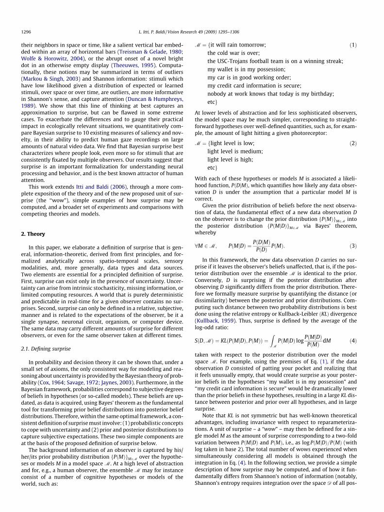
To illustrate how surprise arises when data is observed, con-sider a human observer who just turned a television set on, notknowing which channel it is tuned to. The observer has a numberof co-existing hypotheses or models about which channel may beon, for example, MTV, CNN, FOX, BBC, etc. (Fig. 1). Over the courseof viewing the first few video frames of the unknown channel(here, CNN), the observer’s beliefs in each hypothesis adjust, pro-gressively favoring one channel over the others (leading to a higherprior probability for CNN in left panel). Consider next what hap-pens if yet another video frame of the same program is observed(Fig. 1, top right), intuitively an unsurprising event. Through Bayes-ian update, the new frame only minimally alters the observer’s be-liefs, with the posterior distribution of beliefs over models showinga slightly reinforced belief into the correct channel at the expenseof the others. In contrast, if a frame of snow was suddenly observed(Fig. 1, middle right), intuitively this should be a very surprisingevent, as it may signal storm, earthquake, toddler’s curiosity, elec-tronic malfunction, or a military putsch. Through Bayesian update,this observation would yield a large shift between the prior andposterior distributions of beliefs, with the posterior now stronglyfavoring a snow model (and possible associated earthquake, mal-function, etc. hypotheses), correspondingly reducing belief in allother television channels. In sum, unsurprising data yields littledifference between posterior and prior distributions of beliefs overmodels, while surprising data yields a large shift: in mathematicalterms, an event is surprising when the distance between posteriorand prior distributions of beliefs over all models is large (see Eq.(4)).

While at onset snow is surprising (Fig. 1, middle right), aftersustained viewing it quickly becomes boring to most humans. In-deed, no more surprise arises after the observer’s beliefs have sta-bilized towards strongly favoring the snow model over all others(Fig. 1, bottom right). Thus surprise resolves the classical paradoxthat random snow, although in the long term the most boring of

all television programs, carries the largest amount of Shannoninformation. This paradox arises from the fact that there are manymore possible random images than there exists natural images.Thus, the entropy of snow is higher than that of natural scenes(Field, 2005). Even when the observer knows to expect snow, everyindividual frame of snow carries a large amount of Shannon infor-mation. Indeed, in a sample recording of 20,000 video frames fromtypical television programs, presumably of interest to millions ofwatchers, we measured approximately 20 times less Shannoninformation per second than in matched random snow clips, aftercompression to constant-quality MPEG4 to adaptively eliminateredundancy in both cases (Table 1). The situation was reversedwhen wemeasured that snow clips carried about 17 times less sur-prise per second than the television clips, evaluated using the aver-age, over space and time, of the output of the surprise metricpresented with our human experiments. Note that a clip whereall frames are black would practically carry no Shannon informa-tion and yield no surprise. Thus, more informative data may not al-ways be more important, interesting, worthy of attention, orsurprising; in fact, the most interesting or surprising data may of-ten carry intermediate amounts of Shannon information, betweenfully predictable data (black frames) and completely unpredictabledata (snow frames).

2.3. Simple example of surprise computation

One class of examples where surprise can be computed ex-actly consists of contingency tables of any size. Consider for in-stance a parent who has two competing internal models orhypotheses about a new television channel, the first, M, accord-ing to which that new channel is appropriate for children, andthe second, M, according to which it is not. Assume that initiallyour observer is undecided and equally split across both models,that is, P!M" # P!M" = 1/2. Next consider two possible dataobservations, D1, a TV program that contains some nudity, andD2, one that does not, with, for instance, P(D1) = (D2) = 1/2. Final-ly, assume that the observer initially believes that observingnudity is three times more likely on a channel that is inappropri-ate for children.

The initial beliefs of our observer may thus be tabulated asfollows:

D1 D2

M a = 1/8 c = 3/8M b = 3/8 d = 1/8

where the table verifies the above specifications, in thatP!D1" # a$ b # 1=2, P!D2" # c $ d # 1=2, P!M" # a$ c # 1=2,P!M" # b$ d # 1=2, and P!D1;M" # b # 3% P!D1;M" # 3% a. As-sume that D1 is observed (a program with some nudity). SinceP!D1" # 1=2, this observation carries & log P!D1" # 1 bit of Shannoninformation (remember that the logarithm should be taken in base2 for all numerical applications). The posterior probabilities of Mand M are

P!MjD1" #P!M;D1"

P!M;D1" $ P!M;D1"#

aa$ b

#14

and !5"

P!MjD1" #P!M;D1"

P!M;D1" $ P!M;D1"# b

a$ b# 3

4!6"

That is, observing D1 (a program with some nudity) shifted the ob-server’s initial indecision between M and M, now favoring M (thenew TV channel is inappropriate for children) overM (it is appropri-ate) by a factor 3. The amount of surprise resulting from this shift,

L. Itti, P. Baldi / Vision Research 49 (2009) 1295–1306 1297

first considering only model M, is S!D1;M" # log P!MjD1"P!M" # &1:00

wow. Similarly, with respect to M, the surprise is

S!D1;M" # log P!MjD1"P!M"

# 0:58 wows. After averaging over the model

family M # fM;Mg weighted by the posterior (Eq. 2), the total sur-prise experienced by the observer is

S!D1;M" # P!MjD1"S!D1;M" $ P!MjD1"S!D1;M" !7"

# aa$ b

loga

!a$ b"!a$ c"$ ba$ b

logb

!a$ b"!b$ d"!8"

' 0:19wows: !9"

The new beliefs of the observer may hence be tabulated as fol-lows, using the posterior resulting from our above observation asnew prior:

D1 D2

M a0= 1/16 c

0= 3/16

M b0= 7/16 d

0= 5/16

Consider next what happens if D1 is observed once more. Weintuitively expect this second observation to carry less surprisethan the previous one, since our observer now already fairlystrongly believes that the new TV channel is inappropriate, andobserving nudity once again should only incrementally consolidatethat belief. Indeed, proceeding as above, the total surprise nowexperienced by the observer is S!D1;M" # 0:07 wows, nearly threetimes less than on the previous observation.

2.4. Analytical computations of surprise with N data points

Exponential Family. Consider a family of models M parameter-ized by w with likelihood P!DjM" # P!Djw". By definition, the con-jugate prior P!M" # P!w" has the same functional form as thelikelihood. In this case, by Bayes’ theorem, the posterior also hasthe same functional form. While surprise can be computed withany prior, conjugate priors are useful for their mathematical sim-plicity and ease of implementation during Bayesian learning,

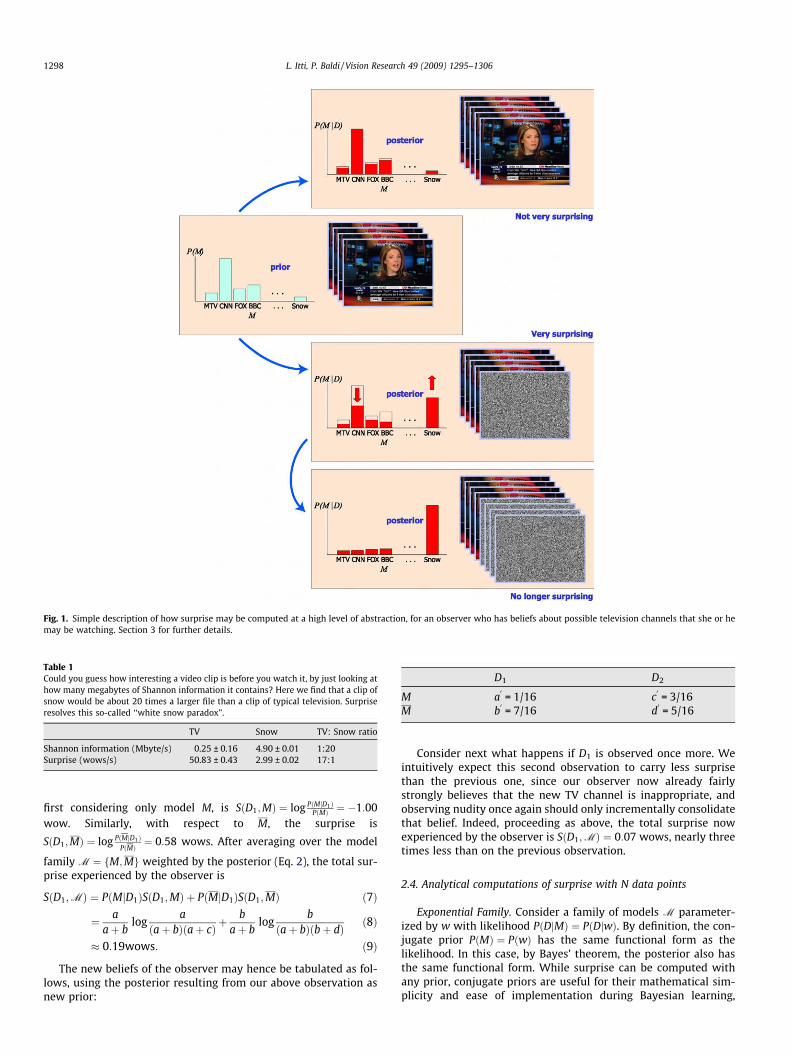
Fig. 1. Simple description of how surprise may be computed at a high level of abstraction, for an observer who has beliefs about possible television channels that she or hemay be watching. Section 3 for further details.

Table 1Could you guess how interesting a video clip is before you watch it, by just looking athow many megabytes of Shannon information it contains? Here we find that a clip ofsnow would be about 20 times a larger file than a clip of typical television. Surpriseresolves this so-called ‘‘white snow paradox”.

TV Snow TV: Snow ratio

Shannon information (Mbyte/s) 0.25 ± 0.16 4.90 ± 0.01 1:20Surprise (wows/s) 50.83 ± 0.43 2.99 ± 0.02 17:1

1298 L. Itti, P. Baldi / Vision Research 49 (2009) 1295–1306

where the posterior at one iteration becomes the prior of the fol-lowing iteration.

A likelihood is in the exponential family with parameter vectorw if it can be expressed in the form, for a single datum d

P!djw" # h!d"c!w" expXk

i#1

hi!w"ti!d" !

!10"

With N independent data points (D # d1; . . . ;dN),

P!Djw" # (c!w")NYN

j#1

h!dj"" #

expXk

i#1

hi!w"Ti!D" !

!11"

letting Ti!D" #PN

j#1ti!dj" be the sufficient statistics. Most commondistributions belong to the exponential family. The conjugate priorhas a similar exponential form

P!w;ai" # C expXk

i#1

aihi!w" !

!12"

parameterized by the ai’s. Using Bayes’ theorem, the posterior hasthe same exponential form with normalizing constant C

0and

a0i # ai $ Ti!D". Calculation of surprise yields

S!D;M" # logC0

C&Xk

i#1

Ti!D"E(hi!w") !13"

where E(hi!w") is the expectation of hi!w"with respect to the poster-ior. Surprise can be rewritten as:

S!D;M" # N

log c!w"$ < logh!d" > & < log P!d" >

&Xk

i#1

< ti!d" > E(hi!w")!

!14"

where <> denotes averages over the data points. Thus in general,for large N, surprise grows linearly with the number of data points.Below is an application.

Binary Data Modeled as a Series of Independent and Identical CoinTosses (Binomial Model). The family M of models is parameterizedby the probability 0 6 w 6 1 of observing ‘‘heads” on a coin toss,thus encompasses models of biased coins (small and large w val-ues) and of fair coins (w # 0:5). The conjugate prior is the Betaprior P!w;a; b" # Cwa&1!1&w"b&1 with C # C!a$ b"=(C!a"C!b")and parameters a, b. With a number n of heads observed after toss-ing a coin N times, the posterior is also a Beta distribution witha0 # a$ n and b0 # b$ !N & n". Integrating over models, surprise is

S!D;M" # logC 0

C& n(W!a$ b$ N" &W!a$ n")

& !N & n"(W!a$ b$ N" &W!b$ N & n") !15"

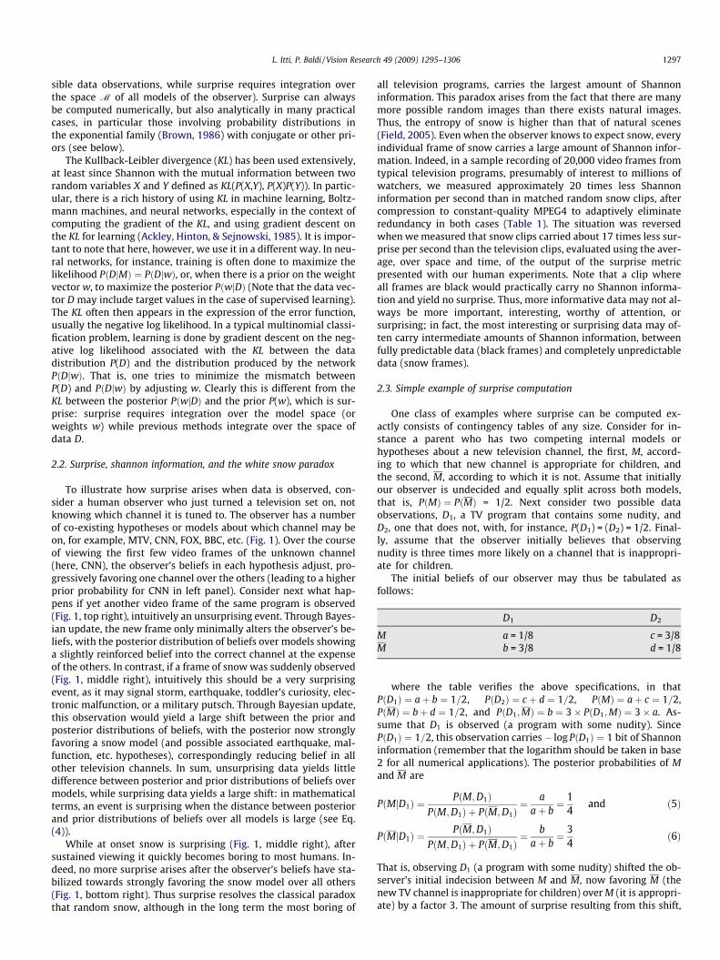
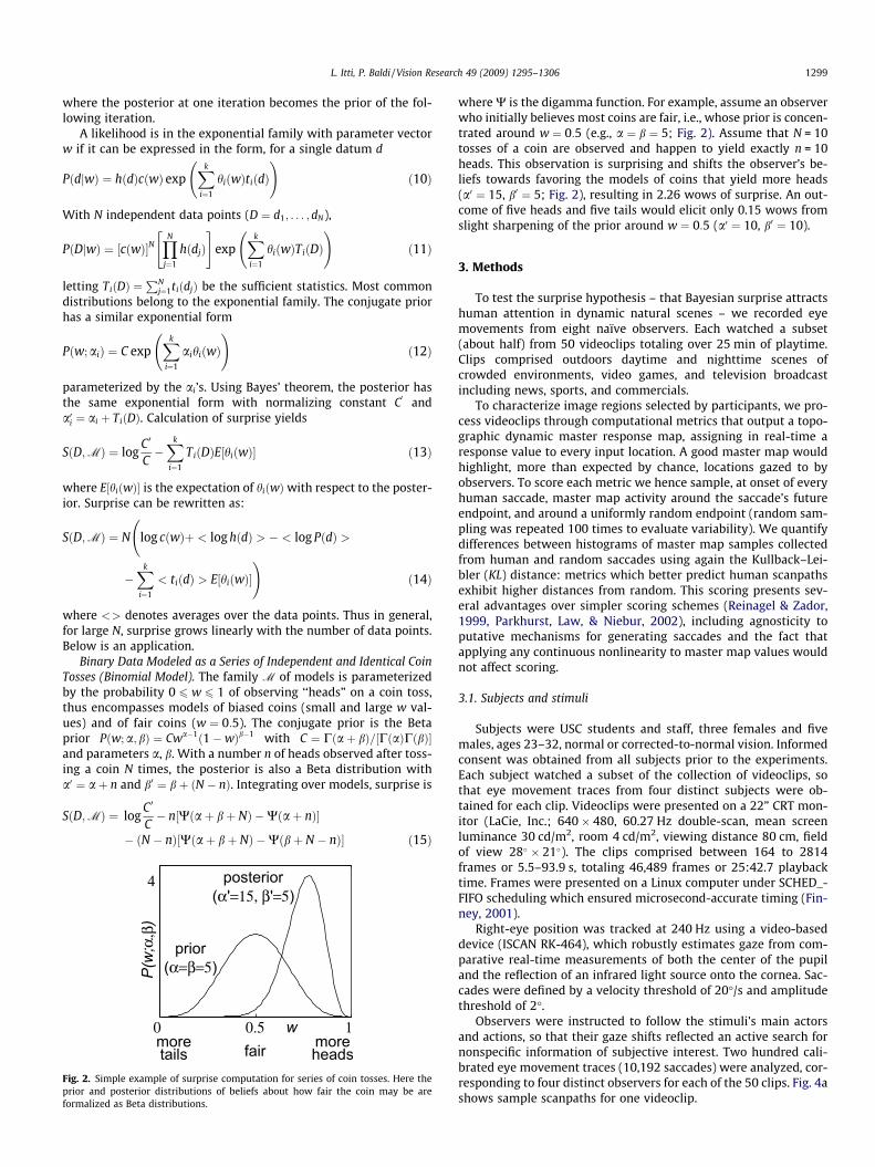
whereW is the digamma function. For example, assume an observerwho initially believes most coins are fair, i.e., whose prior is concen-trated around w # 0:5 (e.g., a # b # 5; Fig. 2). Assume that N = 10tosses of a coin are observed and happen to yield exactly n = 10heads. This observation is surprising and shifts the observer’s be-liefs towards favoring the models of coins that yield more heads(a0 # 15, b0 # 5; Fig. 2), resulting in 2.26 wows of surprise. An out-come of five heads and five tails would elicit only 0.15 wows fromslight sharpening of the prior around w # 0:5 (a0 # 10, b0 # 10).

3. Methods

To test the surprise hypothesis – that Bayesian surprise attractshuman attention in dynamic natural scenes – we recorded eyemovements from eight naïve observers. Each watched a subset(about half) from 50 videoclips totaling over 25 min of playtime.Clips comprised outdoors daytime and nighttime scenes ofcrowded environments, video games, and television broadcastincluding news, sports, and commercials.

To characterize image regions selected by participants, we pro-cess videoclips through computational metrics that output a topo-graphic dynamic master response map, assigning in real-time aresponse value to every input location. A good master map wouldhighlight, more than expected by chance, locations gazed to byobservers. To score each metric we hence sample, at onset of everyhuman saccade, master map activity around the saccade’s futureendpoint, and around a uniformly random endpoint (random sam-pling was repeated 100 times to evaluate variability). We quantifydifferences between histograms of master map samples collectedfrom human and random saccades using again the Kullback–Lei-bler (KL) distance: metrics which better predict human scanpathsexhibit higher distances from random. This scoring presents sev-eral advantages over simpler scoring schemes (Reinagel & Zador,1999, Parkhurst, Law, & Niebur, 2002), including agnosticity toputative mechanisms for generating saccades and the fact thatapplying any continuous nonlinearity to master map values wouldnot affect scoring.

3.1. Subjects and stimuli

Subjects were USC students and staff, three females and fivemales, ages 23–32, normal or corrected-to-normal vision. Informedconsent was obtained from all subjects prior to the experiments.Each subject watched a subset of the collection of videoclips, sothat eye movement traces from four distinct subjects were ob-tained for each clip. Videoclips were presented on a 22” CRT mon-itor (LaCie, Inc.; 640% 480, 60.27 Hz double-scan, mean screenluminance 30 cd/m2, room 4 cd/m2, viewing distance 80 cm, fieldof view 28* % 21*). The clips comprised between 164 to 2814frames or 5.5–93.9 s, totaling 46,489 frames or 25:42.7 playbacktime. Frames were presented on a Linux computer under SCHED_-FIFO scheduling which ensured microsecond-accurate timing (Fin-ney, 2001).

Right-eye position was tracked at 240 Hz using a video-baseddevice (ISCAN RK-464), which robustly estimates gaze from com-parative real-time measurements of both the center of the pupiland the reflection of an infrared light source onto the cornea. Sac-cades were defined by a velocity threshold of 20"/s and amplitudethreshold of 2".

Observers were instructed to follow the stimuli’s main actorsand actions, so that their gaze shifts reflected an active search fornonspecific information of subjective interest. Two hundred cali-brated eye movement traces (10,192 saccades) were analyzed, cor-responding to four distinct observers for each of the 50 clips. Fig. 4ashows sample scanpaths for one videoclip.

Fig. 2. Simple example of surprise computation for series of coin tosses. Here theprior and posterior distributions of beliefs about how fair the coin may be areformalized as Beta distributions.

L. Itti, P. Baldi / Vision Research 49 (2009) 1295–1306 1299

Sampling of master map values around human or random sac-cade targets used a circular aperture of diameter 5.6", approximat-ing the size of the fovea and parafovea. Saccade initiation latencywas accounted for by subjecting the master maps to a temporallow-pass filter with time constant s # 500 ms. This provided anupper bound, allowing the analysis to compensate for delays be-tween the physical appearance of stimuli on the screen and thestart of human saccades. The random sampling process was re-peated 100 times, yielding the (very small) error bars of the ran-dom histograms of Fig. 5.

Note that instead of using a uniform random sampling, the ran-dom saccade distribution could also have been derived by ran-domly shuffling the human saccades (Tatler, Baddeley, &Gilchrist, 2005). However, it is important to understand that usingsuch biased random distribution would confer particular knowl-edge to the random sampling process: general knowledge aggre-gated over the human dataset under study would be exploited todecide how random samples are to be selected. Our computationalgaze prediction metrics do not have any such knowledge about thehuman dataset, and do not have any built-in spatial bias, central orotherwise (except, for some metrics, a slight bias against the ex-treme image borders due to boundary conditions on the filters ap-plied to the images). Hence, we here chose to retain knowledge-free computational and random metrics, rather than to contami-nate them with knowledge about the dataset under study.

3.2. Simulations

Dynamic master maps generated by the computational gazeprediction metrics were 40% 30 lattices of metric responses com-puted over 16% 16 image patches, given 640% 480 stimuli. Themaster maps were internally updated at a rate of 10,000 frames/s(simulated time, actual CPU time was much longer), receivingnew input video frames every 33.185 ms. Simulations were parall-elized across Beowulf clusters of computers, totaling in excess ofone CPU-year to evaluate all computational metrics against our41.5 GB of raw video data and 1,542,752 eye movement samples.

3.3. Human-derived metric

With our clips and instructions, observers agreed with eachother quite often on where to look (Fig. 4b). Hence our data pre-sents ample opportunity for characterizing in the image spacewhat most strongly attracted human observers. An upper-boundKL score can be computed from a human-derived metric, whosemaster map is built, at every video frame, from eye movementpositions of the three observers other than that under test(Fig. 4c). Computational metrics are expected to yield KL scores be-tween zero (chance level) and this upper bound ofKL # 0:679 + 0:011 reflecting inter-observer consistency. To buildthe human-derived maps, a Gaussian blob with r # 3 master mappixels (4.5") was continuously painted at each of the eye positionsof the three observers other than that under test, with some forget-ting provided by the master map’s temporal low-pass filter. Highmetric responses were hence sampled if and only if a saccade ofthe observer under test was aimed to approximately a locationwhere other observer(s) were currently looking. Because this met-ric is not predictive like the others, sampling occurred when a sac-cade ended (and other humans were expected to also be reachingthe endpoint) rather than when it started (and other humans pos-sibly also started).

3.4. Static metrics

The simplest computational metrics tested only exploit localand static image properties. The variance metric computes local

variance of pixel luminance within 16% 16 image patches(Reinagel & Zador, 1999). The Shannon entropy metric computesthe entropy of the local histogram of grey-levels in 16% 16 imagepatches (Privitera & Stark, 2000). The DCT-based (Discrete CosineTransform) information metric similarly computes in imagepatches the number of DCT coefficients above detection threshold,for the luminance and two chrominance channels (Itti, Koch, & Nie-bur, 1998). The color, intensity and orientation contrast metrics arederived from reduced versions of our previously proposed bottom-up saliency metric (Itti & Koch, 2001). They compute local contrastin each feature dimension using difference-of-Gaussian center-sur-round contrast detectors operating at six different spatial scales.

3.5. Dynamic and saliency metrics

The flicker and motion metrics rely on the same center-sur-round architecture as for color, intensity, and orientation. The sal-iency metric combines intensity contrast (six feature maps), red/green and blue/yellow color opponencies (12 maps), four orienta-tion contrasts (24 maps), flicker (six maps) and motion energy infour directions (24 maps), totaling 72 feature maps. Central tothe saliency metric and each of its center-surround feature chan-nels is neurally-inspired non-classical spatial competition for sal-iency (Sillito, Grieve, Jones, Cudeiro, & Davis, 1995; Itti & Koch,2001), by which distant active locations in each feature map inhibiteach other, giving rise to pop-out and attentional capture (Wolfe &Horowitz, 2004). Thus, these metrics are not necessarily attractedto locally information-rich image regions, as many highly informa-tive regions will be discarded if they resemble their neighbors. Forthis reason, these metrics typically yielded sparser maps than thecontrast, entropy, and DCT-based information metrics, which arepurely local. These metrics represent biologically-plausible heuris-tics to an outlier detection metric described below.

3.6. Surprise and outlier metrics

The surprise metric retains the 72 raw feature detection mech-anisms of the saliency metric (but without the non-classical com-petition for saliency), and attaches local surprise detectors to eachlocation in each of the 72 feature maps. Surprise detectors computeboth local temporal surprise (generalizing outliers-based temporalnovelty) and spatial surprise (generalizing outliers-based spatialsaliency).

In our implementation, image patches are described by a 72Dfeature vector representing the responses from the 72 low-levelfeature channels (color, motion, etc. at six spatial scales). A modelof an image patch, then, is a 72D vector of 1D Poisson random vari-ables, under the assumption that each low-level feature detectoroutputs 1D trains of Poisson-distributed spikes in response to vi-sual stimulation (Softky & Koch, 1993). We consider the modelfamily that comprises all possible such 72D vectors of Poissonmodels, parameterized by a single 72D Poisson rate vector. For in-stance, patches of motionless vs. trembling foliage correspond totwo different models, described by two vectors of 72 Poisson firingrates (with, among other differences, lower rates for motion fea-tures in the motionless foliage model). Note that with these simplemodels, there is no single explicit model Msnow that can capturerandom snow. Rather, when snow is observed, the prior quickly be-comes uniform, indicating that every model is believed to beequally bad and that the observer does not have any strong beliefin favor of any one model. More complex models (Doretto, Chiuso,Wu, & Soatto, 2003) could be used as well, without affecting thetheory.

Consider a neuron at a given location in one of the 72 fea-ture maps, receiving Poisson spikes as inputs from low-levelfeature detectors. We compute surprise independently in that

1300 L. Itti, P. Baldi / Vision Research 49 (2009) 1295–1306

feature map and at that location using a family of models whichare all the 1D Poisson distributions for all possible firing ratesk > 0.

Using the theory of surprise outlined above, we consider conju-gate priors, whereby the posterior belongs to the same functionalfamily as the prior. In such case, the posterior at one video framecan directly serve as prior for the next frame, as is customary inBayesian learning. Thus, we use for P!M" a functional form suchthat P!MjD" has the same functional form when D is Poisson-dis-tributed. It is easy to show that P!M" satisfying this property isthe Gamma probability density:

P!M!k"" # c!k;a;b" # baka&1e&bk

C!a" !16"

with shape a > 0, inverse scale b > 0, and C!:" the Euler Gammafunction. Given an observation D # k at one of our surprise detec-tors and prior density c!k;a;b", the posterior c!k;a0; b0" obtainedby Bayes’ theorem is also a Gamma density, with:

a0 # a$ k and b0 # b$ 1 !17"

To prevent these from increasing unbounded over time, we add aforgetting factor 0 < f < 1, yielding:

a0 # fa$ k and b0 # fb$ 1 !18"

f preserves the prior’s mean a=b but increases its variance a=b2,embodying relaxation of belief in the prior’s precision; our simula-tions use f # 0:7, based on a reproduction of neural recordings fromMüller et al. (1999). Local temporal surprise ST resulting from theupdate is computed exactly using the KL divergence to quantifythe differences between posterior and prior distributions overmodels:

ST!D;M" # KL!c!k;a0; b0"; c!k;a; b""

# &a$ a log b0

b$ log

C!a"C!a0"

$ ba0

b0 $ !a0 & a"W!a0" !19"

with W!:" the digamma function. Spatial surprise SS is computedsimilarly. At every visual location, a Gamma neighborhood prior iscomputed as the weighted combination of priors from local models,over a large neighborhood with 2D Difference-of-Gaussians profile(r$ # 20 and r& # 3 feature map pixels, i.e., 29* and 4:5* resp.).As new data arrives, spatial surprise is the KL between the posteriorneighborhood distribution after update by local samples from theneighborhood’s center, and the prior. Temporal and spatial surprise

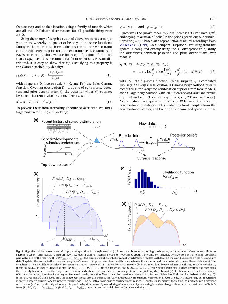
Fig. 3. Hypothetical implementation of surprise computation in a single neuron. (a) Prior data observations, tuning preferences, and top-down influences contribute toshaping a set of ‘‘prior beliefs” a neuron may have over a class of internal models or hypotheses about the world. For instance, M may be a set of Poisson processesparameterized by the rate k, with fP!M"gM2M # fP!k"gk2IR$, the prior distribution of beliefs about which Poisson models well describe the world as sensed by the neuron. Newdata D updates the prior into the posterior using Bayes’ theorem. Surprise quantifies the difference between the posterior and prior distributions over the model classM. Theremaining panels detail how surprise differs from conventional model fitting and outlier-based novelty. (b) In standard iterative Bayesian model fitting, at every iteration N,incoming data DN is used to update the prior fP!MjD1;D2; . . . ;DN&1"gM2M into the posterior fP!MjD1;D2; . . . ;DN"gM2M. Freezing this learning at a given iteration, one then picksthe currently best model, usually using either a maximum likelihood criterion, or a maximum a posteriori one (yieldingMMAP shown). (c) This best model is used for a numberof tasks at the current iteration, including outlier-based novelty detection. New data is then considered novel at that instant if it has low likelihood for the best model (e.g., Db

N

is more novel than DaN). This focus onto the single best model presents obvious limitations, especially in situations where other models are nearly as good (e.g.,M, in panel (b)

is entirely ignored during standard novelty computation). One palliative solution is to consider mixture models, but this just amounts to shifting the problem into a differentmodel class. (d) Surprise directly addresses this problem by simultaneously considering all models and by measuring how data changes the observer’s distribution of beliefsfrom fP!MjD1;D2; . . . ;DN&1"gM2M to fP!MjD1;D2; . . . ;DN"gM2M over the entire model class M (orange shaded area).

L. Itti, P. Baldi / Vision Research 49 (2009) 1295–1306 1301

are combined additively to yield the final surprise metric. Addi-tional implementation details have been described previously (Itti& Baldi, 2005, 2006).

The outlier detection metric uses exactly the same Poissonmodels and low-level visual features as the surprise metric, butfundamentally differs from surprise in that it focuses onto the sin-gle best model at a given moment, instead of simultaneously con-sidering all models like the surprise metric. Thus, at every locationin every feature map, the best Poisson model M!kbest" given the ob-served data to date is considered, and is used to compute the like-lihood of the new data sample, yielding:

O!D;M!kbest"" #1

P!DjM!kbest""& 1: !20"

Thus, a data observation D which is an outlier, that is, has lowlikelihood P!DjM!kbest"" ' 0 given the currently best model, yieldsa large response, while an inlier data observation with highP!DjM!kbest" yields a lower response.

Fig. 3 illustrates how surprise differs from the notions of sal-iency and novelty based on outliers and Shannon information, byexamining a hypothetical implementation of surprise computationin a single neuron.

4. Results

We compare the ten computational metrics described above,which encompass and extend the state-of-the-art found in previ-ous studies, to Bayesian surprise (Table 2). The first six metricsquantify static image properties while the remaining four, andBayesian surprise, also respond to dynamic events. The first threemetrics compute local variance, Shannon entropy, and DCT-based(discrete cosine transform) information within 16% 16 imagepatches, as previously proposed to characterize attractors of hu-man gaze over static images (Reinagel & Zador, 1999; Privitera &Stark, 2000; Itti et al., 1998). We find that humans are significantly

attracted by image regions with higher metric responses (Fig. 5, Ta-ble 2). However, these purely local metrics typically respond vigor-ously at numerous visual locations. Hence they are poorly specificand yield relatively low KL scores between humans and random:while humans preferentially gaze towards locations with highmetric responses, such locations are often so numerous that highmetric responses are also collected at random saccade targets.

The next three metrics increase specificity by focusing on spa-tial image outliers in the dimensions of color, intensity, and orien-tation, using heuristic biologically-inspired center-surrounddetectors operating at six spatial scales. These metrics yield sparsermaps, as local responses are inhibited unless they contrast withneighboring regions. While we find that humans also significantlygaze towards regions with outlier color, intensity, and orientation,these metrics do not score substantially better than the previousthree.

The next two metrics consider the dimensions of flicker (onsets/offsets of light intensity) and directional motion energy, againemploying six center-surround scales, and hence measure spatio-temporal novelty. Both score equivalently well and significantlyhigher than the static metrics (nearly 20% better than the best sta-tic metric, entropy), providing a quantitative evaluation of thestronger impact of dynamic features onto human attentional selec-tion over natural video scenes.

The last three metrics – biologically-inspired saliency, outlierdetection, and surprise – employ a common front-end which con-sists of a set of linear filters tuned to the five features of color,intensity, orientation, flicker, and motion at six spatial scales (Itti& Koch, 2001). They differ in the computations applied to the out-puts of these linear detectors to yield a master map. The biologi-cally-inspired saliency metric implements a heuristic detection ofspatial and temporal outliers in each of the low-level feature chan-nels and spatial scales: non-linear competitive interactions be-tween distant visual locations, mimicking the non-classicalsurround suppression effects observed in primary visual cortex(Sillito et al., 1995; Itti et al., 1998), enhance isolated or outlierstimuli while suppressing more extended regions with high linearfilter outputs. Because it considers both static and dynamic fea-tures, our saliency metric combines both notions of spatial saliencyand temporal novelty into a generalized biologically-inspired mea-sure of saliency. It scores better than any of the single visual fea-tures taken in isolation, suggesting that all features do contributeto human gaze allocation.

The explicit outlier detection metric retains the same front-endas the saliency metric, but instead of biologically-inspired long-range interactions it explicitly computes likelihood of the incomingpixel data given an adaptive model for that data at every locationin each of the feature maps. This metric yields a strong outputwhen incoming data is an outlier (low likelihood) given the adap-tive model (Methods). Hence this metric exactly computes outlierprobabilities instead of relying on biologically-plausible heuristicsas used in the saliency metric. We find that explicit outlier detec-tion and biologically-inspired saliency score equally well, suggest-ing that the neural competitive interactions in the saliency metricwell approximate a true detection of outliers.

Finally we evaluate the surprise metric, which retains the rawlinear visual features of the saliency and outlier detection metrics,but attaches surprise detectors to every location in each of the fea-ture maps. This metric quantifies low-level surprise in imagepatches over space and time, and at this point does not accountfor cognitive beliefs of our human observers, nor does it attemptto consider high-level, possibly semantically-rich, models for thevideo frames (such as the models of television channels discussedin Methods). Rather, the surprise metric assumes a family of simplemodels for image patches and computes surprise from shifts in thedistribution of beliefs about which models better describe the

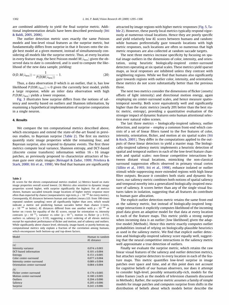
Table 2KL scores for the eleven computational metrics studied. (a) Metrics based on staticimage properties overall scored lowest. (b) Metrics also sensitive to dynamic imageproperties scored higher, with surprise significantly the highest. For all metricsshown, humans saccaded towards image locations of higher metric response moreoften than expected by chance (nonparametric sign tests, p < 10&100 for every metric).Consequently, KL distances between human and random (mean+S.D. from 100-timesrepeated random sampling) were all significantly higher than zero, which wouldindicate a metric not predicting human saccades better than chance (t-tests,p < 10&100 or better). KL distances differed from one another with p < 10&100 orbetter on t-tests for equality of the KL scores, except for orientation vs. intensitycontrasts (p < 10&12), variance vs. color (p < 10&9), motion vs. flicker (p P 0:15),outliers vs. saliency (p P 0:10), suggesting a strict ordering of all eleven metricsexcept for equivalent performance of flicker and motion, and of saliency and outliers.While significantly above chance level, obviously, image-based, or purely bottom-up,computational metrics only explain a fraction of the correlation among humans,which encompasses both bottom-up and top-down factors.

Model Human to randomKL distance

(a)Intensity variance 0.074 ± 0.003DCT-based information 0.101 ± 0.004Entropy 0.151 ± 0.005Color center-surround 0.077 ± 0.004Intensity center-surround 0.089 ± 0.004Orientation center-surround 0.084 ± 0.004

(b)Flicker center-surround 0.179 ± 0.005Motion center-surround 0.180 ± 0.005Outliers 0.204 ± 0.006Saliency 0.205 ± 0.006Surprise 0.241 ± 0.006

1302 L. Itti, P. Baldi / Vision Research 49 (2009) 1295–1306

patches (Methods). Notably, the models used in the surprise metricare the same as in the outlier detection metric. The only differencebetween these two metrics is that one detects outliers based oncomputing likelihood while the other computes surprise. Conse-quently, any difference in performance at predicting human gazepatterns cannot be due to the low-level front-end or class of mod-els used, but must reflect a difference between computing outliersand computing surprise.

We find that the surprise metric significantly outperforms theoutlier and all other computational metrics (p < 10&100 or betteron t-tests for equality of KL scores), scoring nearly 20% better thanthe second-best metric (saliency) and 60% better than the best sta-tic metric (entropy). Surprising stimuli often substantially differfrom simple feature outliers; for example, a shower of randomly-colored pixels continually excites all low-level feature detectorsand outlier detection mechanisms, but rapidly becomesunsurprising.

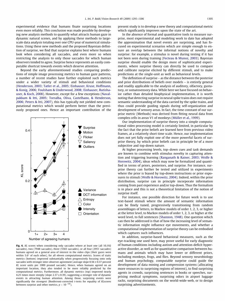
Clearly, in our and previous eye-tracking experiments, in somesituations potentially interesting targets were more numerous

than in others. With many possible targets, different observersmay orient towards different locations, making it more difficultfor a single metric to accurately predict all observers. To investi-gate this, we consider (Fig. 6) subsets of human saccades whereat least two, three, or all four observers simultaneously agreedon a general location of interest. Observers could have agreedbased on bottom-up factors (e.g., only one visual location had strik-ingly interesting image appearance at that time), top-down factors(e.g., only one object qualified as the main actor), or both (e.g., asingle actor was present who also had distinctive appearance).Irrespectively of the cause for agreement, it indicates consolidatedbelief that a location was attractive. While overall the KL scores ofall metrics improved when progressively focusing the analysisonto only those consensus locations, dynamic metrics improvedmore steeply, indicating that stimuli which more reliably attractedall observers carried more flicker, motion, saliency, and surprise(Fig. 6). Surprise remained significantly the best metric to charac-terize these agreed-upon attractors of human gaze (p < 10&100 orbetter on t-tests for equality of KL scores).

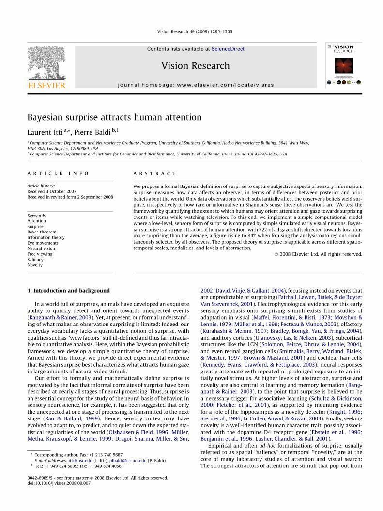
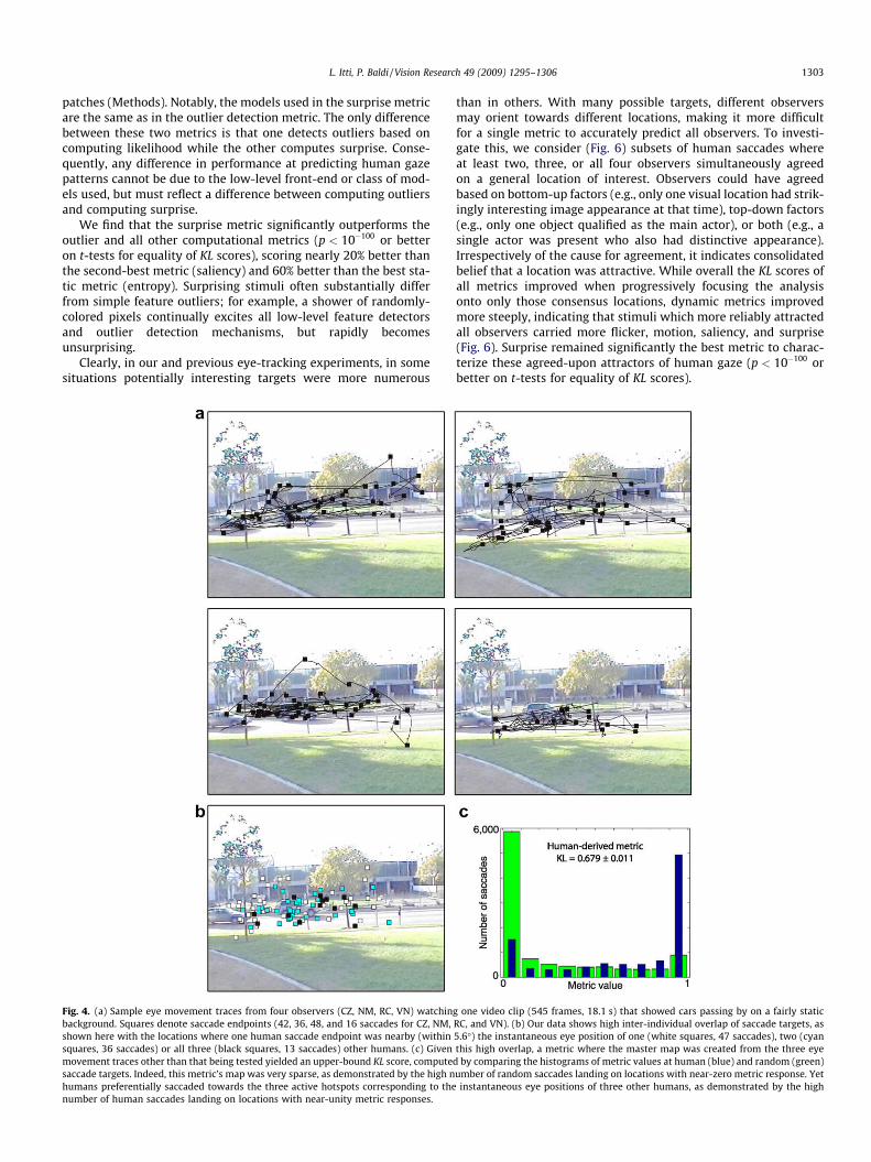
Fig. 4. (a) Sample eye movement traces from four observers (CZ, NM, RC, VN) watching one video clip (545 frames, 18.1 s) that showed cars passing by on a fairly staticbackground. Squares denote saccade endpoints (42, 36, 48, and 16 saccades for CZ, NM, RC, and VN). (b) Our data shows high inter-individual overlap of saccade targets, asshown here with the locations where one human saccade endpoint was nearby (within 5.6") the instantaneous eye position of one (white squares, 47 saccades), two (cyansquares, 36 saccades) or all three (black squares, 13 saccades) other humans. (c) Given this high overlap, a metric where the master map was created from the three eyemovement traces other than that being tested yielded an upper-bound KL score, computed by comparing the histograms of metric values at human (blue) and random (green)saccade targets. Indeed, this metric’s map was very sparse, as demonstrated by the high number of random saccades landing on locations with near-zero metric response. Yethumans preferentially saccaded towards the three active hotspots corresponding to the instantaneous eye positions of three other humans, as demonstrated by the highnumber of human saccades landing on locations with near-unity metric responses.

L. Itti, P. Baldi / Vision Research 49 (2009) 1295–1306 1303

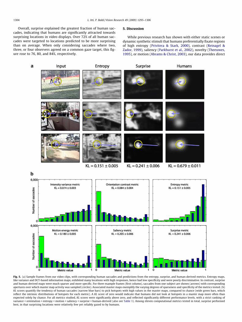
Overall, surprise explained the greatest fraction of human sac-cades, indicating that humans are significantly attracted towardssurprising locations in video displays. Over 72% of all human sac-cades were targeted to locations predicted to be more surprisingthan on average. When only considering saccades where two,three, or four observers agreed on a common gaze target, this fig-ure rose to 76, 80, and 84%, respectively.

5. Discussion

While previous research has shown with either static scenes ordynamic synthetic stimuli that humans preferentially fixate regionsof high entropy (Privitera & Stark, 2000), contrast (Reinagel &Zador, 1999), saliency (Parkhurst et al., 2002), novelty (Theeuwes,1995), or motion (Abrams & Christ, 2003), our data provides direct

Fig. 5. (a) Sample frames from our video clips, with corresponding human saccades and predictions from the entropy, surprise, and human-derived metrics. Entropy maps,like variance and DCT-based information maps, exhibited many locations with high responses, hence had low specificity and were poorly discriminative. In contrast, surpriseand human-derived maps were much sparser and more specific. For three example frames (first column), saccades from one subject are shown (arrows) with correspondingapertures over which master map activity was sampled (circles). Associated master maps exemplify the varying degrees of sparseness and specificity of the metrics tested. (b)KL scores quantify the tendency of human saccades (narrow blue bars) to pick hotspots with high values in the master maps, compared to chance (wide green bars, whichreflect the intrinsic distributions of hotspots for each metric). A KL score of zero would indicate that humans did not look at hotspots in a master map more often thanexpected solely by chance. For all metrics studied, KL scores were significantly above zero, and reflected significantly different performance levels, with a strict ranking ofvariance < orientation < entropy < motion < saliency < surprise < human-derived (also see Table 1). Among eleven computational metrics tested in total, surprise performedbest, in that surprising locations were relatively few yet reliably gazed to by humans.

1304 L. Itti, P. Baldi / Vision Research 49 (2009) 1295–1306

experimental evidence that humans fixate surprising locationseven more reliably. This conclusion was made possible by develop-ing new analysis methods to quantify what attracts human gaze indynamic natural scenes, and by applying these methods to large-scale data analysis totaling over one CPU-year of numerical simula-tions. Using these new methods and the proposed Bayesian defini-tion of surprise, we find that surprise explains best where humanslook when considering all saccades, and even more so whenrestricting the analysis to only those saccades for which humanobservers tended to agree. Surprise hence represents an easily com-putable shortcut towards events which deserve attention.

Beyond the early aforementioned studies comparing predic-tions of simple image processing metrics to human gaze patterns,a number of recent studies have further exploited such metricsunder a wider variety of stimuli and behavioral conditions(Henderson, 2003; Tatler et al., 2005; Einhauser, Kruse, Hoffmann,& Konig, 2006; Foulsham & Underwood, 2008; Einhauser, Rutisha-user, & Koch, 2008). However, except for a few exceptions (Naval-pakkam & Itti, 2005; Torralba, Oliva, Castelhano, & Henderson,2006; Peters & Itti, 2007), this has typically not yielded new com-putational metrics which would perform better than the previ-ously proposed ones. Hence an important contribution of the

present study is to develop a new theory and computational metricwhich significantly improves upon the state of the art.

In the absence of formal and quantitative tools to measure sur-prise, most experimental and modeling work to date has adoptedthe approximation that novel events are surprising, and has fo-cused on experimental scenarios which are simple enough to en-sure an overlap between the informal notions of novelty andsurprise: for example, a stimulus is novel during testing if it hasnot been seen during training (Fecteau & Munoz, 2003). Bayesiansurprise should enable the design more of sophisticated experi-ments, where surprise theory can directly be used to compareand calibrate surprise elicited by different stimuli, and to makepredictions at the single-unit as well as behavioral levels.

The definition of surprise – as the distance between the posteriorand prior distributions of beliefs over models – is entirely generaland readily applicable to the analysis of auditory, olfactory, gusta-tory, or somatosensory data. While here we have focused on behav-ior rather than detailed biophysical implementation, it is worthnoting that detecting surprise in neural spike trains does not requiresemantic understanding of the data carried by the spike trains, andthus could provide guiding signals during self-organization anddevelopment of sensory areas. In fact, the time constant of our sur-prise metric (Methods) was derived from fitting neural data fromcomplex cells in areas V1 of monkeys (Müller et al., 1999).

Our implementation of surprise theory into a simple computa-tional video processing model is certainly limited, in particular bythe fact that the prior beliefs are learned here from previous videoframes, at a relatively short time scale. Hence, our implementationdoes not yet fully exploit one of the more powerful facets of sur-prise theory, by which prior beliefs can in principle be of a moresubjective and top-down nature.

At higher processing levels, top–down cues and task demandsare known to combine with stimulus novelty in capturing atten-tion and triggering learning (Ranganath & Rainer, 2003; Wolfe &Horowitz, 2004), ideas which may now be formalized and quanti-fied in terms of priors, posteriors, and surprise. For instance, sur-prise theory can further be tested and utilized in experimentswhere the prior is biased by top-down instructions or prior expo-sures to stimuli (Wolfe & Horowitz, 2004). Indeed, within the priordistribution, surprise can in principle incorporate informationcoming from past experience and/or top-down. Thus the formalismis in place and this is not a theoretical limitation of the notion ofsurprise itself.

For instance, one possible direction for future work is to usetext-based stimuli where the amount of semantic informationcan be finely tuned, progressively transitioning from randomassemblages of letters, to Markov models of order 1, 2, 3, or higherat the letter level, to Markov models of order 1, 2, 3, or higher at theword level, to full sentences (Shannon, 1948). One question whichcan then be addressed is that of how the increasing level of seman-tic information might influence eye movements, and whether acomputational implementation of surprise theory can be embodiedwhich captures such influences.

In addition, surprise-based behavioral measures, such as theeye-tracking one used here, may prove useful for early diagnosticof human conditions including autism and attention-deficit hyper-active disorder, as well as for quantitative comparison between hu-mans and animals which may have lower or different priors,including monkeys, frogs, and flies. Beyond sensory neurobiologyand human psychology, computable surprise could guide thedevelopment of data mining and compression systems (allocatingmore resources to surprising regions of interest), to find surprisingagents in crowds, surprising sentences in books or speeches, sur-prising medical symptoms, surprising odors in airport luggageracks, surprising documents on the world-wide-web, or to designsurprising advertisements.

Fig. 6. KL scores when considering only saccades where at least one (all 10,192saccades), two (7948 saccades), three (5565 saccades), or all four (2951 saccades)humans agreed on a general area of interest in the video clips (their gazes werewithin 5.6" of each other), for all eleven computational metrics. Scores of staticmetrics (bottom) improved substantially when progressively focusing onto onlysaccades with stronger inter-observer agreement (average slope 0.56 ± 0.37 percentKL score units per 1000 pruned saccade). Hence, when humans agreed on animportant location, they also tended to be more reliably predicted by thecomputational metrics. Furthermore, all dynamic metrics (top) improved nearly4.25 times more steeply (slope 2.37 ± 0.39), suggesting a stronger role of dynamicevents in attracting human attention. Among those, surprising events weresignificantly the strongest (Bonferroni-corrected t-tests for equality of KLscoresbetween surprise and other metrics, p < 10&100).

L. Itti, P. Baldi / Vision Research 49 (2009) 1295–1306 1305

Acknowledgments

Supported by NSF, DARPA, HFSP, and NGA (L.I.), and NIH andNSF (P.B.). We thank UCI’s Institute for Genomics and Bioinformat-ics and USC’s HPCC center for access to their computing clusters,both used to carry out the model predictions reported here. Theauthors affirm that the views expressed herein are solely theirown, and do not represent the views of the United States govern-ment or any agency thereof.

References

Abrams, R. A., & Christ, S. E. (2003). Motion onset captures attention. PsychologicalScience, 14(5), 427–432.

Ackley, D. H., Hinton, G. E., & Sejnowski, T. J. (1985). A learning algorithm forBoltzmann machines. Cognitive Science, 9, 147–169.

Benjamin, J., Li, L., Patterson, C., Greenberg, B. D., Murphy, D. L., & Hamer, D. H.(1996). Population and familial association between the D4 dopamine receptorgene and measures of Novelty seeking. Nature Genetics, 12(1), 81–84.

Bradley, J., Bonigk, W., Yau, K. W., & Frings, S. (2004). Calmodulin permanentlyassociates with rat olfactory CNG channels under native conditions. NatureNeuroscience, 7(7), 705–710.

Brown, L. D. (1986). Fundamentals of statistical exponential families. Hayward, CA:Institute of Mathematical Statistics.

Brown, S. P., & Masland, R. H. (2001). Spatial scale and cellular substrate of contrastadaptation by retinal ganglion cells. Nature Neuroscience, 4(1), 44–51.

Cox, R. T. (1964). Probability, frequency and reasonable expectation. AmericanJournal of Physics, 14, 1–13.

David, S. V., Vinje, W. E., & Gallant, J. L. (2004). Natural stimulus statistics alter thereceptive field structure of v1 neurons. Journal of Neuroscience, 24(31),6991–7006.

Doretto, G., Chiuso, A., Wu, Y., & Soatto, S. (2003). Dynamic textures. InternationalJournal of Computer Vision, 51(2), 91–109.

Dragoi, V., Sharma, J., Miller, E. K., & Sur, M. (2002). Dynamics of neuronal sensitivityin visual cortex and local feature discrimination. Nature Neuroscience, 5(9),883–891.

Duncan, J., & Humphreys, G. W. (1989). Visual search and stimulus similarity.Psychological Reveiw, 96(3), 433–458.

Ebstein, R. P., Novick, O., Umansky, R., Priel, B., Osher, Y., Blaine, D., et al.(1996). Dopamine D4 receptor (D4DR) exon III polymorphism associatedwith the human personality trait of Novelty seeking. Nature Genetics, 12(1),78–80.

Einhauser, W., Kruse, W., Hoffmann, K. P., & Konig, P. (2006). Differences of monkeyand human overt attention under natural conditions. Vision Research, 46(8-9),1194–1209.

Einhauser, W., Rutishauser, U., & Koch, C. (2008). Task-demands can immediatelyreverse the effects of sensory-driven saliency in complex visual stimuli. Journalof Vision, 8(2), 201–219.

Fairhall, A. L., Lewen, G. D., Bialek, W., & de Ruyter Van Steveninck, R. R. (2001).Efficiency and ambiguity in an adaptive neural code. Nature, 412(6849),787–792.

Fecteau, J. H., & Munoz, D. P. (2003). Exploring the consequences of the previoustrial. Nature Reviews. Neuroscience, 4(6), 435–443.

Field, D.J. 2005. Entropy, visual non-linearities and the higher-order statistics ofnatural scenes. In: Proceedings of CVR Vision Conference.

Finney, S. A. (2001). Real-time data collection in Linux: A case study. BehaviorResearch Methods Instruments and Computers, 33, 167–173.

Fletcher, P. C., Anderson, J. M., Shanks, D. R., Honey, R., Carpenter, T. A., Donovan, T.,et al. (2001). Responses of human frontal cortex to surprising events arepredicted by formal associative learning theory. Nature Neuroscience, 4(10),1043–1048.

Foulsham, T., & Underwood, G. (2008). What can saliency models predict about eyemovements? Spatial and sequential aspects of fixations during encoding andrecognition. Journal of Vision, 8(2), 601–617.

Henderson, J. M. (2003). Human gaze control during real-world scene perception.Trends in Cognitive Sciences, 7(11), 498–504.

Itti, L., & Baldi, P. 2005. A Principled Approach to Detecting Surprising Events inVideo. Proceedings in IEEE Conference on Computer Vision and PatternRecognition (CVPR), 631–637.

Itti, L., & Baldi, P. (2006). Bayesian surprise attracts human attention. Advances inneural information processing systems (19). Cambridge, MA.: MIT Press. pp. 547–554 NIPS*2005.

Itti, L., & Koch, C. (2001). Computational modeling of visual attention. NatureReviews Neuroscience, 2(3), 194–203.

Itti, L., Koch, C., & Niebur, E. (1998). A model of saliency-based visual attention forrapid scene analysis. IEEE Transactions on Pattern Analysis and MachineIntelligence, 20(11), 1254–1259.

Jaynes, E. T. (2003). Probability theory. The logic of science. Cambridge UniversityPress.

Kennedy, H. J., Evans, M. G., Crawford, A. C., & Fettiplace, R. (2003). Fast adaptationof mechanoelectrical transducer channels in mammalian cochlear hair cells.Nature Neuroscience, 6(8), 832–836.

Knight, R. (1996). Contribution of human hippocampal region to novelty detection.Nature, 383(6597), 256–259.

Kullback, S. (1959). Information theory and statistics. New York: Wiley.Kurahashi, T., & Menini, A. (1997). Mechanism of odorant adaptation in the

olfactory receptor cell. Nature, 385(6618), 725–729.Li, S., Cullen, W. K., Anwyl, R., & Rowan, M. J. (2003). Dopamine-dependent

facilitation of LTP induction in hippocampal CA1 by exposure to spatial novelty.Nature Neuroscience, 6(5), 526–531.

Lusher, J. M., Chandler, C., & Ball, D. (2001). Dopamine D4 receptor gene (DRD4) isassociated with Novelty seeking (NS) and substance abuse: The saga continues.Molecular Psychiatry, 6(5), 497–499.

Maffei, L., Fiorentini, A., & Bisti, S. (1973). Neural correlate of perceptual adaptationto gratings. Science, 182(116), 1036–1038.

Markou, M., & Singh, S. (2003). Novelty detection: A review – Part 1: Statisticalapproaches. Signal Processing, 83(12), 2481–2497.

Movshon, J. A., & Lennie, P. (1979). Pattern-selective adaptation in visual corticalneurones. Nature, 278(5707), 850–852.

Müller, J. R., Metha, A. B., Krauskopf, J., & Lennie, P. (1999). Rapid adaptation invisual cortex to the structure of images. Science, 285(5432), 1405–1408.

Navalpakkam, V., & Itti, L. (2005). Modeling the influence of task on attention. VisionResearch, 45(2), 205–231.

Olshausen, B. A., & Field, D. J. (1996). Emergence of simple-cell receptive fieldproperties by learning a sparse code for natural images. Nature, 381(6583),607–609.

Parkhurst, D., Law, K., & Niebur, E. (2002). Modeling the role of salience in theallocation of overt visual attention. Vision Research, 42(1), 107–123.

Peters, R.J., & Itti, L. 2007 (Jun). Beyond bottom-up: Incorporating task-dependentinfluences into a computational model of spatial attention. In: Proc. IEEEConference on Computer Vision and Pattern Recognition (CVPR).

Privitera, C. M., & Stark, L. W. (2000). Algorithms for defining visual regions-of-interest: comparison with eye fixations. IEEE Transactions on Pattern Analysisand Machine Intelligence, 22(9), 970–982.

Ranganath, C., & Rainer, G. (2003). Neural mechanisms for detecting andremembering novel events. Nature Reviews. Neuroscience, 4(3), 193–202.

Rao, R. P., & Ballard, D. H. (1999). Predictive coding in the visual cortex: A functionalinterpretation of some extra-classical receptive-field effects. NatureNeuroscience, 2(1), 79–87.

Reinagel, P., & Zador, A. M. (1999). Natural scene statistics at the centre of gaze.Network, 10, 341–350.

Savage, L. J. (1972). The foundations of statistics. New York: Dover. First Edition in1954.

Schultz, W., & Dickinson, A. (2000). Neuronal coding of prediction errors. AnnualReview of Neuroscience, 23, 473–500.

Shannon, C. E. (1948). A mathematical theory of communication. Bell SystemTechnical Journal, 27, 379–423. 623–656.

Sillito, A. M., Grieve, K. L., Jones, H. E., Cudeiro, J., & Davis, J. (1995). Visual corticalmechanisms detecting focal orientation discontinuities. Nature, 378(6556),492–496.

Smirnakis, S. M., Berry, M. J., Warland, D. K., Bialek, W., & Meister, M. (1997).Adaptation of retinal processing to image contrast and spatial scale. Nature,386(6620), 69–73.

Softky, W. R., & Koch, C. (1993). The highly irregular firing of cortical cells isinconsistent with temporal integration of random EPSPs. Journal ofNeuroscience, 13(1), 334–350.

Solomon, S. G., Peirce, J. W., Dhruv, N. T., & Lennie, P. (2004). Profound contrastadaptation early in the visual pathway. Neuron, 42(1), 155–162.

Stern, C. E., Corkin, S., Gonzalez, R. G., Guimaraes, A. R., Baker, J. R., Jennings, P. J.,et al. (1996). The hippocampal formation participates in novel pictureencoding: Evidence from functional magnetic resonance imaging. Proceedingsof the National Academy of Sciences of the United States of America, 93(16),8660–8665.

Tatler, B. W., Baddeley, R. J., & Gilchrist, I. D. (2005). Visual correlates of fixationselection: Effects of scale and time. Vision Research, 45(5), 643–659.

Theeuwes, J. (1995). Abrupt luminance change pops out; abrupt color change doesnot. Percept Psychophys, 57(5), 637–644.

Torralba, A., Oliva, A., Castelhano, M. S., & Henderson, J. M. (2006). Contextualguidance of eye movements and attention in real-world scenes: The role ofglobal features in object search. Psychological Reveiw, 113(4), 766–786.

Treisman, A. M., & Gelade, G. (1980). A feature-integration theory of attention.Cognitive Psychology, 12(1), 97–136.

Ulanovsky, N., Las, L., & Nelken, I. (2003). Processing of low-probability sounds bycortical neurons. Nature Neuroscience, 6(4), 391–398.

Wolfe, J. M., & Horowitz, T. S. (2004). What attributes guide the deployment ofvisual attention and how do they do it? Nature Reviews. Neuroscience, 5(6),495–501.

1306 L. Itti, P. Baldi / Vision Research 49 (2009) 1295–1306