Bayesian VAR Analysis - U-M Personal World Wide Web …lkilian/SVARch05.pdf · Chapter 5 Bayesian VAR Analysis GiventhefactthatVARmodelsareestimatedoncomparativelyshortsamples and

Chapter 5

Bayesian VAR Analysis

Given the fact that VAR models are estimated on comparatively short samplesand hence tend to be imprecisely estimated, many users of VAR models aresympathetic to the idea of imposing additional structure in estimation. Forexample, shrinking parameter estimates toward specific values may help reducethe variance of unrestricted LS estimators. The Bayesian approach provides aformal framework for incorporating such extraneous information in estimationand inference. It also facilitates the inclusion of extraneous economic informa-tion about the VAR model parameters that would be difficult to incorporate infrequentist analysis.

The ideas behind the Bayesian approach differ fundamentally from the fre-quentist approach. Broadly speaking, frequentists condition on the existenceof a parameter vector, say θ, that governs the DGP from which the observedsample of data is thought to have been obtained. The objective is to infer thevalue of θ from this sample. Whereas the data are stochastic, the parametervector θ is nonstochastic. Probability statements refer to the properties of theestimator of θ in repeated sampling.

In contrast, in Bayesian analysis, the parameter vector θ is treated as stochas-tic, whereas the data are considered nonstochastic. Bayesians are concernedwith modeling the researcher’s beliefs about θ. These beliefs are expressed inthe form of a probability distribution. The Bayesian probability concept is asubjective probability concept. It does not require a repeated sampling exper-iment. Moreover, the nature of the DGP is immaterial for inference on theparameter of interest because inference conditions on the observed data.

The researcher’s subjective beliefs about the value of the parameter vectorθ before inspecting the data are summarized in the form of a prior probabilitydistribution (or prior for short) for θ. This prior information is formally com-bined with the information contained in the data, as captured by the likelihoodfunction of the model, to form the posterior probability distribution (or simply

c© 2016 Lutz Kilian and Helmut LutkepohlPrepared for: Kilian, L. and H. Lutkepohl, Structural Vector Autoregressive Analysis, Cam-bridge University Press, Cambridge.

139

140 CHAPTER 5. BAYESIAN VAR ANALYSIS

posterior) for θ. This posterior conveys everything the researcher knows aboutthe model parameters after having looked at the data.

Frequentists are aware that they do not know the DGP for a given set ofvariables, but they evaluate the properties of their methods under the assump-tion that there exists a true parameter vector θ that can be objectively defined.They postulate a DGP and then conduct their analysis, as if this model structureincluding any distributional assumptions were correct. In contrast, Bayesiansdo not need to take a stand on the DGP. However, their formal framework forderiving and evaluating the posterior requires users to articulate their prior be-liefs in the form of a prior probability distribution. It also involves assuming aspecific distribution (or family of distributions) for the data, when evaluatingthe likelihood.

The choice between frequentist and Bayesian methods depends on the pref-erences of the user. In practice, convenience may also play an important role. Insome situations frequentist methods are easier to deal with, and in other casesBayesian methods are more convenient. It has to be kept in mind, however,that these approaches not only may produce numerically different answers inmany cases, but that their interpretation is fundamentally different, even whenthe estimates coincide numerically. Since Bayesian methods are frequently usedin VAR analysis, it is essential to have at least a basic understanding of thisapproach.

Although Bayesian methods often require extensive computations, they havebecome quite popular for VAR analysis because the cost of computing has de-creased dramatically over the last decades. Moreover, new methods and algo-rithms have broadened the applicability of Bayesian methods. In Section 5.1,we briefly review some basics of the Bayesian methodology and terminologyand then discuss Bayesian methods commonly used in VAR analysis. Section5.2 reviews some commonly used prior specifications for the reduced-form VARparameters. There are many good introductory treatments of Bayesian method-ology in general and for macroeconometric analysis in particular. Canova (2007)and Koop and Korobilis (2009) fall in the latter category. Recent surveys in-clude, for example, Ciccarelli and Rebucci (2003), Del Negro and Schorfheide(2011), and Karlsson (2013). The present chapter follows in part Lutkepohl(2005, Section 5.4), Geweke and Whiteman (2006), and Canova (2007).

5.1 Basic Terms and Notation

5.1.1 Prior, Likelihood, Posterior

The Bayesian approach treats the data, y = (y′1, . . . , y′T )′, as given and the

parameter of interest, θ, as unknown. Inference about θ is conditional on thedata. Prior information on θ is assumed to be available in the form of a density.Suppose the prior information is summarized in the prior probability densityfunction (pdf) g(θ) and the sample pdf conditional on a particular value ofthe parameter θ is f(y|θ). The latter function is algebraically identical to

5.1. BASIC TERMS AND NOTATION 141

the likelihood function l(θ|y). The two types of information are combined byapplying Bayes’ theorem, which states that the joint density is

f(θ,y) = g(θ|y)f(y),

and, hence,

g(θ|y) = f(y|θ)g(θ)f(y)

.

Here f(y) denotes the unconditional sample density which is just a normalizingconstant for a given sample y and does not depend on θ. Scaling the posteriorby f(y) ensures that the posterior density integrates to 1. In other words, thejoint sample and prior information can be summarized by a function that isproportional to the likelihood function times the prior density g(θ),

g(θ|y) ∝ f(y|θ)g(θ) = l(θ|y)g(θ), (5.1.1)

where ∝ indicates that the right-hand side is proportional to the left-hand side.The conditional density g(θ|y) is the posterior pdf. It contains all the infor-mation that we have on the parameter vector θ after having updated our priorviews by looking at the data. Thus, the posterior pdf is the basis for estimationand inference. In the next subsection we discuss Bayesian inference within thisgeneral framework in more detail.

5.1.2 Bayesian Estimation and Inference

Point Estimators

Bayesian inference on the parameter vector θ is based on the posterior distribu-tion. Often moments of the posterior distribution are of interest. For example,one may be interested in E(θ|y). The posterior mean is often used as a pointestimator for θ, if the posterior distribution is Gaussian or at least symmetric.More generally one is often interested in expected values of functions of θ. Ifwe are interested in constructing a point estimate of some function h(θ) thatmay be vector-valued or a scalar, we minimize the expected loss of h(θ) basedon some loss function. Denoting this loss function by L(h†, h(θ)), the point

estimate, say h†, is chosen such that

h† = argminh†

∫L(h†, h(θ))g(θ|y)dθ, (5.1.2)

where h† denotes an element of the range of h(θ). For example, if the lossfunction is quadratic and the first two moments of the posterior distributionexist, the point estimate corresponds to the posterior mean. Under alternativeloss functions the median or the mode of the posterior distribution may beused as point estimates. These estimates coincide if the posterior distributionis Gaussian.


Credible Sets

The Bayesian concept corresponding to a confidence set in classical inference isa credible set. For 0 < γ < 1, a (1 − γ)100% credible set for θ with respect tothe posterior g(θ|y) is a set Ω such that

P(θ ∈ Ω|y) =∫Ω

g(θ|y)dθ = 1− γ. (5.1.3)

This set can be estimated by sampling from the posterior distribution. In generalit will not be unique, however. To make the credible set unique, one may chooseΩ such that g(θ|y) ≥ cγ for all θ ∈ Ω, where cγ is the largest number such thatP(θ ∈ Ω|y) = 1 − γ. In other words, one may choose the highest posteriordensity (HPD) set.

Depending on the context, this set may differ numerically from a frequentistconfidence interval or region. Given that the posterior density is partly deter-mined by the prior, the posterior for a specific parameter may, for example, bebimodal, in which case an HPD region may consist of two disjoint sets. Evenif the HPD set and the frequentist confidence set coincide numerically, theirinterpretation is quite different. A (1 − γ)100% confidence interval estimatorasymptotically contains the true parameter value in (1− γ)100% of the cases inrepeated sampling. This means that the true parameter is either in a specificinterval estimate or it is not in this interval. Frequentists cannot say whetherthe true parameter is inside or outside a specific confidence interval estimate,but only that an interval constructed by their method will include the true valuein repeated sampling with probability 1− γ. In contrast, the Bayesian credibleset specifies a region where (1−γ)100% of the probability mass of the posteriordistribution is concentrated. This allows them to make probability statementsabout the parameter of interest, θ, given the data and the stochastic modelof the data. There is no true value of θ for a Bayesian, nor is it consideredimportant what the true value of θ is. The construction of credible sets easilygeneralizes to smooth functions h(θ), the posterior of which may be evaluatedby simulation.

Testing Statistical Hypotheses and Model Comparison

Hypothesis testing is another important part of frequentist statistics. In fre-quentist hypothesis testing, the model specified under the null hypothesis ismaintained unless there is overwhelming evidence against it. Bayesians aretypically not interested in hypothesis testing, but in quantifying the empiricalsupport for alternative models. Typically, Bayesians choose between modelsbased on their posterior odds ratios. Suppose that we want to compare twomodels M1 and M2, for example. Then the posterior odds ratio is

g(M1|y)g(M2|y) =

g(M1)

g(M2)× f(y|M1)

f(y|M2), (5.1.4)

where g(M1)/g(M2) reflects the prior odds and f(y|M1)/f(y|M2) is the Bayesfactor. The Bayes factor is the ratio of the marginal likelihoods or marginal


data densities,

f(y|Mj) =

∫f(y|Mj ,θ)g(θ)dθ, j = 1, 2,

that are obtained by integrating the parameters out of the likelihood function.If the posterior odds ratio is greater than one, this is evidence in favor of modelM1, whereas a posterior odds ratio smaller than one favors M2. Obviously, ifthe prior for all models is the same, the ratio of the marginal likelihoods, knownas the Bayes factor, determines which model is preferred. More generally, ifthere are m alternative models that are regarded as a priori equally likely, thena Bayesian solution would be to select the model with the highest marginallikelihood. This procedure is also applicable if nested models are considered, aswould be the case, for example, in choosing between VAR models of differentlag orders.1

Note that Bayesian model comparison and frequentist hypothesis testinghave quite different interpretations. Frequentist hypothesis testing treats theparameter vector as fixed. A rejection of the null hypothesis in favor of thealternative hypothesis occurs when the sample gives rise to a value of the teststatistic that exceeds the critical value at the chosen significance level. Thechoice of the significance level reflects the user’s definition of reasonable doubt.If there is no evidence against the null hypothesis beyond a reasonable doubt,the test is not informative. Thus, the choice of the null hypothesis matters. Thenull hypothesis is always protected from rejection rather than both hypothesesbeing treated symmetrically.

Although one could make the case for choosing model M1 over M2 if theposterior odds ratio is much larger than one, implementing this rule in practicewould require choosing a threshold value, beyond which a Bayesian would chooseM1 for further analysis and discard M2. Choosing such a threshold would beanalogous to choosing a significance level in frequentist hypothesis testing be-cause eliminating one model from further consideration corresponds to rejectingthe null hypothesis in frequentist testing. Thus, Bayesian model comparison ismore akin to model selection procedures in frequentist statistics (such as theinformation criteria discussed in Chapter 2) than to classical hypothesis testingin that it treats all models under consideration symmetrically.

More generally, many Bayesians view all attempts at choosing between alter-native models as misguided. A common alternative is Bayesian model averaging.Consider m candidate models M1, . . . ,Mm. If interest centers on E(h(θ)), forexample, one averages over the candidate models such that

E(h(θ)) =

m∑i=1

E(h(θ)|y,Mi)g(Mi|y). (5.1.5)

Alternatively, a Bayesian may select the median model. Another choice would

1Even some subsets of the parameter space having measure zero is not a problem forBayesian analysis, as long as the prior probability of the parameters is nonzero, given thatmodels with zero prior probability are of no interest from a Bayesian perspective.


be to select the a posteriori most likely model, i.e., the model with the largestg(Mi|y), i = 1, . . . ,m. Each of these choices reflects a different loss function.

5.1.3 Simulating the Posterior Distribution

Bayesian inference is based on the posterior distribution. That distributionmay not be available in closed form, but often can be simulated using numericalmethods. In this subsection some numerical algorithms are discussed that areuseful for this purpose.

Typically, the objective is to generate random draws θ(1), . . . ,θ(n) from theposterior distribution of the parameters or some function of these parameterssuch as the impulse responses associated with a VAR model. Generating drawsfrom potentially complicated and high-dimensional distributions is an importantpart of Bayesian analysis. Suppose that we are interested in the expectation ofh(θ) which may be a vector or a scalar function. Laws of large numbers suggestthat we can obtain a good approximation to this quantity by drawing at randomθ(1), . . . ,θ(n) from the posterior distribution and noting that

1

n

n∑i=1

h(θ(i))a.s.→ E(h(θ)|y) =

∫h(θ)g(θ|y)dθ. (5.1.6)

The approximation precision increases with the number n of random draws.Simulating the posterior distribution is difficult when this distribution is

nonstandard or unknown. Below we discuss a range of tools designed for suchsituations. We only outline the general ideas to enable the reader to determinewhich algorithm is suitable in a specific situation, without providing the fulldetails. Some of these methods are used in later chapters in the context ofspecific applications. Further details can be found, for example, in Canova(2007, Section 9.5) or Geweke and Whiteman (2006, Section 3).

Direct Sampling

If the joint posterior distribution of all parameters is from a known distribu-tion family, random samples can be generated easily using the random numbergenerators provided in standard software packages. A case in point is Gaussianposterior distributions. Unfortunately, in practice, often the posterior distri-bution is not from a known family, in which case more sophisticated samplingtechniques are required.

Acceptance Sampling

Sometimes the posterior density is not available in closed form, but what isknown is a function that is proportional to the posterior density. A functionthat is proportional to a given density function, but does not integrate to one,is called a kernel of this density function. For example, the product of the priorand the likelihood function, g(θ)l(θ|y), is a kernel of the posterior density. It is


not a density because the area under the function usually does not integrate toone. Denote the kernel of the posterior density g∗(θ|y).

If the underlying distribution is difficult to sample from, we may choosea density gAS(θ) that is easy to sample from and that satisfies gAS(θ) > 0whenever g∗(θ|y) > 0. The function gAS(θ) is called the source density. Toensure strictly positive values of the source density whenever g∗(θ|y) > 0, onemay, for example, choose a normal density for gAS(θ) because this density isstrictly positive on the whole real line. The maximum (or supremum) of theratio of the posterior kernel and the source density is defined as

� = supθ∈{θ|g∗(θ|y)>0}

g∗(θ|y)gAS(θ)

.

Then the ith sample value, θ(i), from the posterior can be obtained by proceedingas follows:

Step 1. Draw a random number u from U(0, 1), the uniform distribution onthe interval (0, 1), and draw θ+ from the distribution corresponding togAS(θ).

Step 2. Retain θ(i) = θ+ if u < g∗(θ+|y)/(� · gAS(θ+)). Otherwise return toStep 1.

It can be shown that this algorithm provides a random sample from theposterior distribution. Clearly, if gAS(θ|y) = g∗(θ|y), then � = 1,

g∗(θ+|y)� · gAS(θ+)

= 1.

Thus, we would retain all draws from the source distribution in Step 2. If,however, the source density is very different from the posterior density such thatit assumes very small values when g(θ|y) is large, then the ratio g∗(θ+|y)/(� ·gAS(θ+)) tends to be small, and only very few draws are accepted. Hence,a large number of draws from the source distribution may be necessary forgenerating a sufficiently large number of draws from the posterior. In otherwords, although the algorithm is general, it can be computationally costly andother algorithms may be preferable.

Importance Sampling

Importance sampling avoids the drawback of having to discard many posteriordraws. Instead, we retain a suitably weighted average of all posterior draws.This proposal dates back at least to Hammersly and Handscomb (1964) andwas first used in the econometrics literature by Kloek and van Dijk (1978).The idea is to generate a sample that facilitates the estimation of the posteriormoments of functions of θ. Suppose again that the function of interest is h(θ)and let gIS(θ) be a proper source density, defined as a density that approximates


g∗(θ|y) and has the same support. Furthermore, define a weighting function asthe ratio of g∗ and gIS ,

w(θ) =g∗(θ|y)gIS(θ)

. (5.1.7)

Then, for θ(1), . . . ,θ(n) randomly drawn from the distribution corresponding togIS(θ), under general conditions, we obtain∑n

i=1 h(θ(i))w(θ(i))∑n

i=1 w(θ(i))

a.s.→ E[h(θ|y)], (5.1.8)

because∫h(θ)g∗(θ|y)dθ =

∫h(θ)

g∗(θ|y)∫g∗(θ|y)dθdθ =

∫ h(θ)g∗(θ|y)gIS(θ)

gIS(θ)dθ∫ g∗(θ|y)gIS(θ)

gIS(θ)dθ.

Thus, a properly weighted set of draws from the source distribution can be usedto approximate the expectation based on the posterior distribution.

Clearly, the advantage of this algorithm over acceptance sampling is thatonly a sample of size n has to be drawn. Since the accuracy of the approximationof the expected value of interest improves with the sample size, it is an obviousadvantage that all sample values can be used directly. It should be noted,however, that finding a good approximation gIS(θ) to the posterior densitymay not be easy. The weights may vary dramatically which may undermine theconvergence properties of the quantity in expression (5.1.8). Thus, importancesampling may not work well, if the posterior distribution is complicated anddifficult to sample from. More recent proposals for generating samples from theposterior therefore involve Markov Chain Monte Carlo methods.

Markov Chain Monte Carlo (MCMC) Methods

MCMC methods use a Markov chain algorithm to generate one long sampleof the parameter vector, the distribution of which converges to the posteriordistribution of the parameters, if the chain runs long enough. The draws of theparameter vector are not independent, however, but serially dependent. Laws oflarge numbers and central limit theorems for dependent samples can be invokedto justify the use of such samples for posterior inference. It should be under-stood, however, that the approximation precision for the posterior moment ofinterest tends to be lower, when the posterior is computed from a dependentsample rather than a random sample. Thus, longer samples may be necessaryfor precise inference. In fact, for the construction of approximately independentsamples from the joint posterior, one may want to work only with every mth

sampled vector, where m is a sufficiently large number. Moreover, a large num-ber of initial sample values (also known as transients or the burn-in sample) areusually discarded to ensure a close approximation of the posterior. Diagnostic


tools for assessing the convergence of the posterior to the target distributionare discussed in Chib (2001), among others. Despite their high computationaldemands, MCMC methods have become quite popular in recent years becausethey are often simpler and more computationally efficient than other samplingmethods. There are several variations of this approach in the literature thatdiffer in the way they choose the ith draw of θ, denoted θ(i), given θ(i−1).

MCMC methods have been known in the literature for a long time. Theyhave become increasingly popular in Bayesian analysis after the publication ofan influential article by Gelfand and Smith (1990). More recent introductoryexpositions are Chib and Greenberg (1995) and Geweke (2005). In the following,the very general Metropolis-Hastings algorithm and the popular Gibbs samplerare presented. The Gibbs sampler can only be used if the posterior can bebroken down in a suitable way. It is very convenient and very efficient if theconditions for its use are satisfied.

Metropolis-Hastings Algorithm The Metropolis-Hastings algorithm is basedon a conditional density, η(θ|θ(i−1)). For a given θ(i−1), a candidate θ+ is drawn

from the distribution corresponding to η(θ|θ(i−1)), and θ(i) = θ+ is chosen withprobability

min

{g(θ+|y)/η(θ+|θ(i−1))

g(θ(i−1)|y)/η(θ(i−1)|θ+), 1

}.

Otherwise θ(i) = θ(i−1). In other words, a draw is accepted with probabilityone if it increases the posterior. Otherwise, it is accepted with a probability lessthan one, the precise value of which depends on how much lower the currentposterior value is compared with the previous draw. It can be shown that thisalgorithm converges to the posterior under general conditions.

There are a number of practical questions related to the Metropolis-Hastingsalgorithm. Of prime importance is, of course, the choice of the conditionaldensity η(θ|θ(i−1)). There are different proposals in the literature. A review canbe found in Chib and Greenberg (1995), for example. Another important issueis the size of the burn-in sample. The question is how many initial draws shouldbe discarded in the construction of the chain. Several criteria are discussed inCowles and Carlin (1996), among others.

Clearly, one would not want to use this algorithm, if computationally sim-pler methods exist. In practice, the Metropolis-Hastings sampler is only usedfor nonstandard problems when there is no alternative. A case in point is the es-timation of VAR parameters that cannot be estimated using the Gibbs samplerof either Waggoner and Zha (2003) or Villani (2009). For example, Giannone,Lenza, and Primiceri (2015) use the Metropolis-Hastings algorithm because ofthe complicated form of the kernel of the posterior distribution of their hy-perparameters. Likewise many time-varying coefficient VAR models requireMetropolis-Hastings sampling.


Gibbs Sampler If the posterior distribution of θ is difficult to sample from,the problem often may be simplified by partitioning the parameter vector suchthat the conditional posterior of one of the subvectors, given the remaining ele-ments, has a known, conventional distribution from which samples can be drawneasily. Consider the simplest case where θ can be partitioned as θ = (θ′(1),θ

′(2))

′

such that g(θ(1)|θ(2),y) and g(θ(2)|θ(1),y) correspond to known distributionsthat can be simulated easily. This case arises in VAR models, for example, if wepartition the parameters into the VAR coefficients and the residual covariance

matrix. In this situation, for given θ(i−1)(2) we may choose θ

(i)(1) by drawing from

g(θ(1)|θ(i−1)(2) ,y) and choose θ

(i)(2) by drawing from g(θ(2)|θ(i)

(1),y), starting from

some initial value θ(0)(2). This simple algorithm converges to the joint posterior

under general conditions.

The Gibbs sampler can be generalized in several ways. First, a generalizationto the case where θ needs to be partitioned into more than two subvectorsto obtain standard conditional posterior distributions is straightforward. Itshould be noted, however, that the Gibbs sampler works very well only whenthe posterior distributions of the different subvectors are independent or at leastnot strongly correlated. This feature should be taken into account in groupingthe parameters. Second, it may happen that some of the conditional posteriordistributions are not from a standard family. As long as at least one conditionaldistribution is obtained that is easy to sample from, the Gibbs sampler is worthconsidering. The other conditional distributions may then be approximated bya Metropolis-Hastings step.

5.2 Priors for Reduced-Form VAR Parameters

In Bayesian analysis an important issue is the specification of the prior for theparameters of interest. Often a prior is specified that simplifies the posterioranalysis. In particular, it is convenient to specify the prior such that the poste-rior is from a known family of distributions. If the prior is chosen such that theposterior has the same functional form as the likelihood function, it is calleda conjugate prior. If the conjugate prior is from the same distribution familyas the likelihood, then it is called a natural conjugate prior. For example, it isshown in Section 5.2.2 that if the likelihood is Gaussian and the prior is alsonormal, then the posterior again has a normal distribution. The Litterman orMinnesota prior is discussed as a special case. The natural conjugate prior forall the parameters is known as the Gaussian-inverse Wishart prior. It is consid-ered in Section 5.2.4, whereas the more computationally convenient independentGaussian-inverse Wishart prior is considered in Section 5.2.5.

When using priors from a known family of distributions, it is still necessaryto specify at least some of the parameters of the prior distribution. This taskis often made easier by imposing additional structure on the prior, reducing thenumber of parameters to be chosen to a handful of so-called hyperparameters.We discuss this idea in Section 5.2.1. In Sections 5.2.2-5.2.5 we consider popu-

5.2. PRIORS FOR REDUCED-FORM VAR PARAMETERS 149

lar choices for the prior distribution of the reduced-form VAR parameters anddiscuss how these distributions may be parameterized with the help of a smallset of hyperparameters.

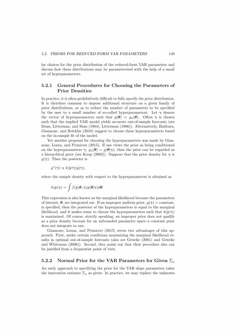
5.2.1 General Procedures for Choosing the Parameters ofPrior Densities

In practice, it is often prohibitively difficult to fully specify the prior distribution.It is therefore common to impose additional structure on a given family ofprior distributions, so as to reduce the number of parameters to be specifiedby the user to a small number of so-called hyperparameters. Let γ denotethe vector of hyperparameters such that g(θ) = gγ(θ). Often γ is chosensuch that the implied VAR model yields accurate out-of-sample forecasts (seeDoan, Litterman, and Sims (1984), Litterman (1986)). Alternatively, Banbura,Giannone, and Reichlin (2010) suggest to choose these hyperparameters basedon the in-sample fit of the model.

Yet another proposal for choosing the hyperparameters was made by Gian-none, Lenza, and Primiceri (2015). If one views the prior as being conditionedon the hyperparameters γ, gγ(θ) = g(θ|γ), then the prior can be regarded asa hierarchical prior (see Koop (2003)). Suppose that the prior density for γ isg(γ). Then the posterior is

g∗(γ) ∝ h(y|γ)g(γ),

where the sample density with respect to the hyperparameters is obtained as

h(y|γ) =∫

f(y|θ,γ)g(θ|γ)dθ.

This expression is also known as the marginal likelihood because the parametersof interest, θ, are integrated out. If an improper uniform prior, g(γ) = constant,is specified, then the posterior of the hyperparameters is equal to the marginallikelihood, and it makes sense to choose the hyperparameters such that h(y|γ)is maximized. Of course, strictly speaking, an improper prior does not qualifyas a prior density because for an unbounded parameter space a constant priordoes not integrate to one.

Giannone, Lenza, and Primiceri (2015) stress two advantages of this ap-proach. First, under certain conditions maximizing the marginal likelihood re-sults in optimal out-of-sample forecasts (also see Geweke (2001) and Gewekeand Whiteman (2006)). Second, they point out that their procedure also canbe justified from a frequentist point of view.

5.2.2 Normal Prior for the VAR Parameters for Given Σu

An early approach to specifying the prior for the VAR slope parameters takesthe innovation variance Σu as given. In practice, we may replace the unknown


Σu by its LS or ML estimate (see, e.g., Litterman (1986)). Understanding thisapproach is also useful for expository purposes.

Consider a normally distributed K-dimensional VAR(p) process yt of theform

yt = ν +A1yt−1 + · · ·+Apyt−p + ut,

where ut ∼ N (0,Σu) is a Gaussian white noise error term. For t = 1, . . . , T , themodel can be written in matrix notation as

Y = AZ + U, (5.2.1)

where Y ≡ [y1, . . . , yT ], A ≡ [ν,A1, . . . , Ap] and Z ≡ [Z0, . . . , ZT−1] with Zt−1 ≡(1, y′t−1, . . . , y

′t−p)

′. Vectorizing the matrix expression (5.2.1), one obtains

y = (Z ′ ⊗ IK)α+ u, (5.2.2)

where α ≡ vec(A), y ≡ vec(Y ), and u ≡ vec(U). Next we discuss two alter-native ways for expressing a normal prior for α under the assumption that thewhite noise covariance matrix Σu is known.

Prior Distribution

Suppose the prior distribution of α is multivariate normal with known mean α∗

and covariance matrix Vα. We write

α ∼ N (α∗, Vα)

and, hence, the prior density is

g(α) =

(1

2π

)K(Kp+1)/2

|Vα|−1/2exp

[−1

2(α−α∗)′V −1

α (α−α∗)]. (5.2.3)

Combining this information with the sample information summarized in theGaussian likelihood function,

l(α|y) =

(1

2π

)KT/2

|IT ⊗ Σu|−1/2

×exp[−1

2[y − (Z ′ ⊗ IK)α]

′(IT ⊗ Σ−1

u )[y − (Z ′ ⊗ IK)α]

],

yields the posterior density

g(α|y) ∝ g(α)l(α|y)∝ exp

{− 1

2

[[V −1/2

α (α−α∗)]′[V −1/2α (α−α∗)]

+ {(IT ⊗ Σ−1/2u )y − (Z ′ ⊗ Σ−1/2

u )α}′

×{(IT ⊗ Σ−1/2u )y − (Z ′ ⊗ Σ−1/2

u )α}]}

. (5.2.4)


Defining

w =

[V−1/2α α∗

(IT ⊗ Σ−1/2u )y

]and W =

[V−1/2α

Z ′ ⊗ Σ−1/2u

],

the exponent in (5.2.4) can be rewritten as

− 12 (w −Wα)′(w −Wα)

= − 12 [(α− α)′W ′W (α− α) + (w −W α)′(w −W α)], (5.2.5)

where

α = (W ′W )−1W ′w = [V −1α +(ZZ ′⊗Σ−1

u )]−1[V −1α α∗+(Z⊗Σ−1

u )y]. (5.2.6)

Note that if the precision matrix V −1α were zero, the expression for the posterior

mean would simplify to that of the unrestricted LS estimator in equation (2.3.2)by noting that

(ZZ ′⊗Σ−1u )−1(Z ⊗Σ−1

u )y = ((ZZ ′)−1Z ⊗ IK)vec(Y ) = vec(Y Z ′(ZZ ′)−1).

The second term on the right-hand side of (5.2.5) does not contain α and there-fore is a constant. Thus,

g(α|y) ∝ exp

[−1

2(α− α)′Σ−1

α (α− α)

],

with α as given in (5.2.6) and

Σα = (W ′W )−1 = [V −1α + (ZZ ′ ⊗ Σ−1

u )]−1. (5.2.7)

The posterior density is easily recognizable as the density of a multivariatenormal distribution with mean α and covariance matrix Σα. In other words,the posterior distribution of α is N (α, Σα). This distribution may be used forinference about α. Sampling from this posterior distribution is particularly easybecause the distribution is of a known form that is easy to draw from.

An Alternative Representation of the Prior Distribution

The prior information on α can equivalently be written as

Cα = c+ e with e ∼ N (0, I), (5.2.8)

where C is a fixed matrix and c is a fixed vector. If C is a K(Kp+1)×K(Kp+1)nonsingular matrix, this expression implies

α ∼ N (C−1c, C−1C−1′), (5.2.9)

which is just the normal prior specified earlier with mean C−1c and covariancematrix (C ′C)−1. Using (5.2.6), the posterior mean can be expressed as

α = [C ′C + (ZZ ′ ⊗ Σ−1u )]−1[C ′c+ (Z ⊗ Σ−1

u )y]. (5.2.10)


Note that under this prior specification there is no need to invert the potentiallylarge covariance matrix Vα. Another practical advantage of this form is that itdoes not require the inversion of C. In fact, C does not have to be a squarematrix.

It is also worth mentioning that the estimator α in (5.2.10) is precisely theGLS estimator obtained from a regression model[

yc

]=

[Z ′ ⊗ IK

C

]α+ ε, ε ∼

(0,

[IT ⊗ Σu 0

0 I

]), (5.2.11)

as pointed out by Theil (1963). Thus, in this case imposing the prior amountsto extending the sample. As in the frequentist setting, adding more observa-tions tends to reduce the variance of the GLS estimator compared with theunrestricted LS estimator, and, hence, increases the estimation efficiency.

In order to make these concepts operational, the prior mean α∗ and the priorcovariance matrix Vα (or, equivalently, C and c) must be specified. If no specificprior knowledge about the parameters is available, then one may use a diffuseGaussian prior by choosing the prior variances very large, so that V −1

α (alsoknown as the precision matrix) becomes very small. In that case the posteriormean is seen to be close to the LS estimator (see (5.2.6)).

The posterior mean can also be interpreted as a shrinkage estimator of αwith the degree of shrinkage determined by V −1

α . If V −1α = 0 is used, the

posterior mean reduces to the LS estimator. Of course, in that case Bayesiananalysis looses its potential advantage of reducing the variance of the parameterestimates. In practice, there are a number of alternative ways of specifyingnontrivial precision matrices. The next subsections discuss the most commonchoices.

Practical Considerations

An important concern in practice is that priors may be inadvertently informa-tive about the parameters of interest. Hence, there has been interest in priorsthat are uninformative. Ideally, assigning equal prior probability to all possibleparameter values would avoid such distortions because in that case the priordensity is just a constant that cancels from the posterior density due to therequirement that the posterior density integrates to one (see (5.1.1)). Unfortu-nately, there is no probability density that is constant over the entire Euclideanspace. Any nonzero, positive constant would integrate to infinity over the wholespace. Hence such a flat prior is not a proper prior. In other words, a trulyuninformative prior for the VAR parameters does not exist.

An alternative is a Gaussian prior with V −1α approaching zero. Such a prior

is also known as a diffuse prior for the VAR parameters. Note, however, thatsuch priors, although they do not seem to restrict the slope parameters much,may still be unintentionally informative for nonlinear functions of the parame-ters such as impulse responses. It should always be kept in mind that a priorthat seems uninformative in one dimension tends to be informative in otherdimensions.


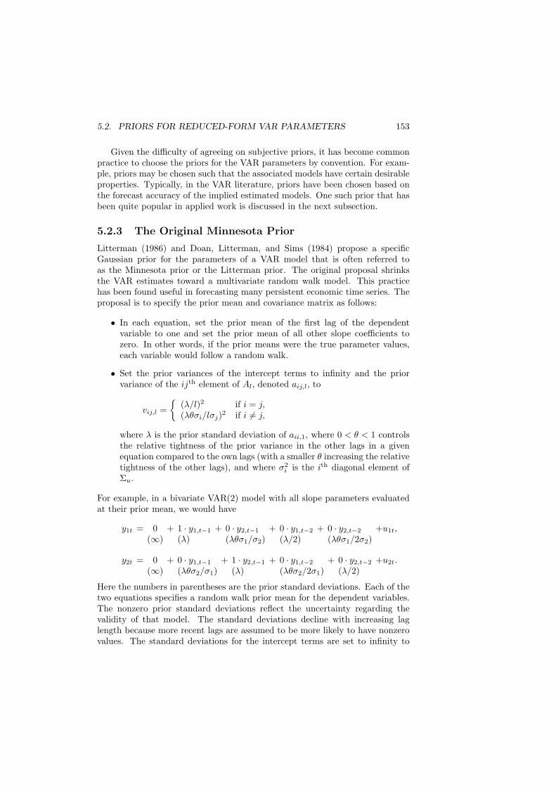
Given the difficulty of agreeing on subjective priors, it has become commonpractice to choose the priors for the VAR parameters by convention. For exam-ple, priors may be chosen such that the associated models have certain desirableproperties. Typically, in the VAR literature, priors have been chosen based onthe forecast accuracy of the implied estimated models. One such prior that hasbeen quite popular in applied work is discussed in the next subsection.

5.2.3 The Original Minnesota Prior

Litterman (1986) and Doan, Litterman, and Sims (1984) propose a specificGaussian prior for the parameters of a VAR model that is often referred toas the Minnesota prior or the Litterman prior. The original proposal shrinksthe VAR estimates toward a multivariate random walk model. This practicehas been found useful in forecasting many persistent economic time series. Theproposal is to specify the prior mean and covariance matrix as follows:

• In each equation, set the prior mean of the first lag of the dependentvariable to one and set the prior mean of all other slope coefficients tozero. In other words, if the prior means were the true parameter values,each variable would follow a random walk.

• Set the prior variances of the intercept terms to infinity and the priorvariance of the ijth element of Al, denoted aij,l, to

vij,l =

{(λ/l)2 if i = j,(λθσi/lσj)

2 if i = j,

where λ is the prior standard deviation of aii,1, where 0 < θ < 1 controlsthe relative tightness of the prior variance in the other lags in a givenequation compared to the own lags (with a smaller θ increasing the relativetightness of the other lags), and where σ2

i is the ith diagonal element ofΣu.

For example, in a bivariate VAR(2) model with all slope parameters evaluatedat their prior mean, we would have

y1t = 0 + 1 · y1,t−1 + 0 · y2,t−1 + 0 · y1,t−2 + 0 · y2,t−2 +u1t,(∞) (λ) (λθσ1/σ2) (λ/2) (λθσ1/2σ2)

y2t = 0 + 0 · y1,t−1 + 1 · y2,t−1 + 0 · y1,t−2 + 0 · y2,t−2 +u2t.(∞) (λθσ2/σ1) (λ) (λθσ2/2σ1) (λ/2)

Here the numbers in parentheses are the prior standard deviations. Each of thetwo equations specifies a random walk prior mean for the dependent variables.The nonzero prior standard deviations reflect the uncertainty regarding thevalidity of that model. The standard deviations decline with increasing laglength because more recent lags are assumed to be more likely to have nonzerovalues. The standard deviations for the intercept terms are set to infinity to


capture our ignorance about the actual values of these parameters. Also, theprior distribution imposes independence across the parameters. Therefore, Vα

is diagonal. Its inverse is

V −1α =

⎡⎢⎢⎢⎢⎢⎢⎢⎢⎢⎢⎢⎢⎢⎢⎢⎢⎢⎣

00

1λ2 0

σ21

(λθσ2)2

σ22

(λθσ1)21λ2

0 22

λ2

22σ21

(λθσ2)2

22σ22

(λθσ1)2

22

λ2

⎤⎥⎥⎥⎥⎥⎥⎥⎥⎥⎥⎥⎥⎥⎥⎥⎥⎥⎦

,

where 0 is also substituted for the inverse of the infinite prior standard deviationof the intercepts.

In terms of expression (5.2.9), the prior for the slope parameters may equiv-alently be specified by choosing

C =

⎡⎢⎢⎢⎢⎢⎢⎢⎢⎢⎢⎣

0 0 1λ 0

0 0 σ1

λθσ2

0 0 σ2

λθσ1

0 0 1λ

0 0 0 2λ

0 0 2σ1

λθσ2

0 0 2σ2

λθσ1

0 0 2λ

⎤⎥⎥⎥⎥⎥⎥⎥⎥⎥⎥⎦and c =

1

λ

⎡⎢⎢⎢⎢⎢⎢⎢⎢⎢⎢⎣

10010000

⎤⎥⎥⎥⎥⎥⎥⎥⎥⎥⎥⎦,

where c = 1λ (vec(I2)

′, 01×4)′ and C is an 8×10 matrix with two leading columns

of zeros and the square roots of the reciprocals of the diagonal elements of Vα

on the main diagonal of the remaining 8× 8 block. Note that in this alternativerepresentation no prior is specified for the intercept.

Practical Issues

The crucial advantage of the Minnesota prior is that it reduces the problem ofspecifying a high-dimensional prior distribution to one of selecting two parame-ters by imposing additional structure on the prior. In specifying the Minnesotaprior, the user has to choose only the two hyperparameters λ and θ. The pa-rameter λ controls the overall prior variance of all VAR coefficients, whereas θcontrols the tightness of the variances of the coefficients of lagged variables otherthan the dependent variable in a given equation. Roughly speaking, θ specifiesthe fraction of the prior standard deviation λ attached to the coefficients ofother lagged variables. A value of θ close to one implies that all coefficients of


lag 1 have about the same prior variance except for a scaling factor intended tocapture differences in the variability of each variable. For example, Litterman(1986) finds that θ = 0.3 and λ = 0.2 works well when using a Bayesian VARmodel for forecasting U.S. macroeconomic variables. For given θ, the shrinkageis determined by λ. Therefore λ is often referred to as the shrinkage parameter.A smaller λ implies a stronger shrinkage towards the prior mean.2

There are also a number of other practical problems that have to be ad-dressed in working with the Minnesota prior. For example, the assumption of aknown Σu is unrealistic in practice. In a strict Bayesian approach, a prior pdfhas to be specified for the elements of Σu. This possibility is discussed in thenext section. A simple alternative is to replace Σu by its LS estimator or itsML estimator,

Σu = Y (IT − Z ′(ZZ ′)−1Z)Y ′/T,

based on the full sample T .Given that the computation of α requires the inversion of the potentially

rather large matrix V −1α +(ZZ ′⊗Σ−1

u ), Bayesian estimation based on the Min-nesota prior has often been performed for each of the K equations of the systemseparately. In that case,

ak = [V −1k + σ−2

k ZZ ′]−1(V −1k a∗k + σ−2

k Zy(k))

is the estimator for the parameters ak of the kth equation, where y(k) ≡ (yk1, . . . , ykT )′.

In other words, a′k is the kth row of A = [ν,A1, . . . , Ap]. Here Vk denotes theprior covariance matrix of ak and a∗k is its prior mean. The unknown σ2

k may

be replaced by the kth diagonal element of Σu.Shrinking the parameters of models of macroeconomic variables toward a

random walk is only plausible for economic time series with stochastic trends.When working with stationary variables, the VAR parameters may be shrunktowards zero instead, as proposed by Lutkepohl (1991, Section 5.4) and imple-mented, for example, in Baumeister and Kilian (2012). In that case, mean-adjusting the data before fitting a VAR model may be useful to avoid havingto specify a prior for the intercept term. Villani (2009) makes the case that amean-adjusted model form may have advantages if prior information is to beimposed on the steady-state of the variables.

Many other modifications of the Minnesota prior have been proposed, de-pending on the needs of the researcher (see, for example, Kadiyala and Karlsson(1997), Sims and Zha (1998), Waggoner and Zha (2003), Banbura, Giannone,and Reichlin (2010), Karlsson (2013)). The main advantage of the Minnesotaprior is that it results in a simple analytically tractable normal posterior dis-tribution, which explains why it has remained popular over the years, despitesome disadvantages. There are alternatives, however. For example, Sims and

2 Rather than selecting λ and θ based on rules of thumb, one could instead treat thesehyperparameters as endogenous and set them to the values that maximize the marginal like-lihood, as proposed by Giannone, Lenza, and Primiceri (2015).


Zha (1998), building on the representation (5.2.11), proposed imposing prior re-strictions on the structural VAR parameters rather than the reduced-form VARparameters (see Chapter 12).

Cointegration and Near Unit Roots

One potential disadvantage of the Litterman prior is that even if all variableshave stochastic trends, it is not clear that shrinking towards a multivariate ran-dom walk as in the Litterman prior is optimal because there may be cointegra-tion between the variables (see Chapter 3). This approach can be rationalizedon the grounds that exact unit roots are events of probability zero in stan-dard Bayesian analysis. Hence, there is no reason to pay special attention tocointegration relations from a Bayesian point of view. Nevertheless the impor-tance of the concept of cointegration and of VECMs in frequentist analysis hasprompted some Bayesians to develop alternative priors that explicitly refer tothe parameters of the VECM form of the VAR.

Consider expressing the VAR model in the VEC representation introducedin Chapter 3,

Δyt = ν +Πyt−1 + Γ1Δyt−1 + · · ·+ Γp−1Δyt−p+1 + ut,

where Π = −(IK −A1 − · · · −Ap). A prior that shrinks Π to zero in the limitreduces the VECM to a VAR model in differences. Such a prior may also besuitable if there are near unit roots (see Chapter 3). A specific prior of thistype, referred to as the sum-of-coefficients prior in Doan, Litterman, and Sims(1984), is implemented by augmenting the observations similar to expression(5.2.11). For the sum-of-coefficients prior we augment Y and Z in model (5.2.1)by

Y∗ = diag(μ1, . . . , μK)/τ

and

Z∗ =

⎡⎢⎢⎢⎣01×K⎡⎢⎣ 1

...1

⎤⎥⎦⊗ diag(μ1, . . . , μK)/τ

⎤⎥⎥⎥⎦ ,

respectively, and consider the vectorized version of the model

[Y, Y∗] = A[Z, Z∗] + [U, E ]

instead of (5.2.11). If the shrinkage parameter τ is small, the prior shrinksthe posterior mean of Π to zero. If τ is very large, the posterior mean of Πis close to the LS estimator. The μk are supposed to capture the potentiallydifferent levels of the ykt. In practice, the sample mean is used as a proxy forμk, although that approach is not, strictly speaking, Bayesian (see Banbura,


Giannone, and Reichlin (2010)). Of course, shrinkage may also be imposed onthe Γi parameters. Such a prior can be imposed by adding further dummyobservations, as described earlier, based on expression (5.2.11). For furthermotivation and discussion of the sum-of-coefficients prior the reader is referredto Sims and Zha (1998).

Bayesian analysis of VECMs is discussed, for example, in Kleibergen andvan Dijk (1994), Kleibergen and Paap (2002), Strachan (2003), and Strachanand Inder (2004). Surveys with many additional references are Koop, Strachan,van Dijk, and Villani (2005) and Karlsson (2013).

An Empirical Illustration

To illustrate the use of the Minnesota prior, we consider a model including quar-terly U.S. GDP deflator inflation (Δπt), the seasonally adjusted unemploymentrate (urt) and the yield on the 3-month Treasury bills (rt) for the period 1953q1- 2006q3, as used by Koop and Korobilis (2009).3 The time series are plottedin Figure 5.1. All three series exhibit considerable persistence, so using theMinnesota prior with shrinkage to a random walk makes sense. To allow forthe possibility that the time series have no unit roots, we alternatively considershrinking all parameters to zero by means of a white noise prior mean.

We consider a VAR(4) model with intercept and impose a conventional Min-nesota prior. Following the example of some earlier studies, the unknown errorvariances are replaced by estimates obtained from fitting univariate AR(4) mod-els to the individual model variables. No estimates of the error covariances arerequired for the specification of the prior. In constructing the posterior, theerror covariance matrix is treated as known and replaced by its LS estimate.

Figure 5.2 illustrates the impact of alternative specifications of the Min-nesota prior on the posterior density of selected structural impulse responses(see Chapter 4). The structural responses are obtained by imposing a recur-sive structure on the impact multiplier matrix with the variables ordered asyt = (Δπt, urt, rt)

′. In particular, the interest rate is ordered last, so the shockto the interest rate equation may be interpreted as a monetary policy shockwith no contemporaneous effect on inflation and unemployment (see Chapter9). Figure 5.2 focuses on the responses of inflation to an unexpected increasein the interest rate (which represents a contractionary monetary policy shock).Following common practice, the figure plots the 10%, 50%, and 90% quantilesof the draws from the posterior distributions of the individual impulse responsecoefficients.

Figure 5.2 illustrates how the choice of the prior affects the structural impulseresponse estimates. The random walk prior mean is used for generating thepanels on the left, and the white noise prior mean is used for the panels on theright. Obviously it makes a difference which prior mean specification is used,

3The data are available on Gary Koop’s webpage athttp://personal.strath.ac.uk/gary.koop/bayes matlab code by koop and korobilis.html.This webpage in addition provides a set of Matlab code for BVAR analysis, modified versionsof which have been used to produce the results below.


1953 1958 1963 1968 1973 1978 1983 1988 1993 1998 20030

10

20Inflation rate

1953 1958 1963 1968 1973 1978 1983 1988 1993 1998 20030

10

20Unemployment rate

1953 1958 1963 1968 1973 1978 1983 1988 1993 1998 20030

10

20Interest rate

Figure 5.1: Quarterly U.S. inflation, unemployment rate, and interest rate for1953q1-2006q3.


0 4 8 12 16 20 24

−0.2

−0.1

0

0.1

0.2Random walk, λ=0.1, θ=0.5

0 4 8 12 16 20 24

−0.2

−0.1

0

0.1


0 4 8 12 16 20 24

−0.2

−0.1

0

0.1


0 4 8 12 16 20 24

−0.2

−0.1

0

0.1

0.2White noise, λ=0.1, θ=0.5

0 4 8 12 16 20 24

−0.2

−0.1

0

0.1


0 4 8 12 16 20 24

−0.2

−0.1

0

0.1


Figure 5.2: Simulated quantiles of inflation responses to monetary policy shocksfor different Minnesota priors (pointwise median and 10% and 90% quantiles ofthe posterior distribution computed from 10,000 draws). The prior standard de-viation for the constant terms is set to 1000 throughout; the standard deviationsof the innovations are replaced by estimates obtained from fitting univariateAR(4) models to each model variable.


but the choice of the hyperparameters λ and θ, which control the prior variance,also is important. A tight prior variance about the random walk prior meanresults in smaller bands around the pointwise medians than a prior with largerλ and θ parameters. Shrinkage to a white noise process makes an even largerdifference, unless the prior variance is large (λ = 1.0, θ = 1.0). In the first twopanels on the right, inflation increases in response to a contractionary monetarypolicy shock. This phenomenon is usually referred to as the price puzzle and hasbeen observed in many structural VAR studies. It is often attributed to omittedvariables. This example illustrates that this puzzle can also be an artifact ofthe choice of the prior. In this example, shrinking the slopes to a white noisemean implies a very different posterior than shrinking to the random walk mean.More generally, one could allow for different prior means in each equation of theVAR model, depending on the order of integration of the individual variables.

5.2.4 The Natural Conjugate Gaussian-Inverse WishartPrior

So far we have replaced the unknown Σu by an estimate. This approach can beimproved upon by specifying a prior not only for the slope parameters, but alsofor Σu. The prior distribution of the innovation covariance matrix must satisfythe constraint that Σu is positive definite. This section discusses such a priorand derives the corresponding posterior.

Let xi ∼ N (0,Σx), i = 1, . . . , n, be K-dimensional independent, identicallydistributed normal random vectors. Then the distribution of

∑ni=1 xix

′i is called

a (K-dimensional) Wishart distribution with parameters Σx and n. We write

n∑i=1

xix′i ∼ WK(Σx, n). (5.2.12)

For univariate standard normal random variables xi,∑n

i=1 x2i has a χ2(n) dis-

tribution, which illustrates that the Wishart distribution can be viewed as amultivariate generalization of a χ2 distribution with n degrees of freedom. IfΩ ∼ WK(Σ, n), then the distribution of Ω−1 depends on Σ−1 and n only. Thelatter distribution is an inverted Wishart or inverse Wishart distribution withparameters Σ−1 and n, and is abbreviated as

Ω−1 ∼ IWK(Σ−1, n).

Suppose that for the VAR(p) model (5.2.1) with Gaussian innovations, ut ∼N (0,Σu), we specify the priors

α|Σu ∼ N (α∗, Vα = V ⊗ Σu) (5.2.13)

and

Σu ∼ IWK(S∗, n), (5.2.14)


such that Σ−1u ∼ WK(S−1

∗ , n).4 Expressing the prior covariance matrix of α asa Kronecker product V ⊗Σu simplifies the posterior distribution, and we obtaina Gaussian-inverse Wishart distribution

α|Σu,y ∼ N (α, Σα), Σu|y ∼ IWK(S, τ), (5.2.15)

where (5.2.7) implies that

Σα = [(V −1 ⊗ Σ−1u ) + (ZZ ′ ⊗ Σ−1

u )]−1 = (V −1 + ZZ ′)−1 ⊗ Σu.

Substituting V ⊗ Σu for Vα into expression (5.2.6) yields

α = [(V −1 ⊗ Σ−1u ) + (ZZ ′ ⊗ Σ−1

u )]−1[(V −1 ⊗ Σ−1u )α∗ + (Z ⊗ Σ−1

u )y]

= [(V −1 + ZZ ′)−1 ⊗ Σu][V−1 ⊗ Σ−1

u , Z ⊗ Σ−1u ]

[α∗

y

]=

((V −1 + ZZ ′)−1[V −1, Z]⊗ IK

)vec[A∗, Y ].

Hence, the posterior mean can be written in matrix notation as

A = (A∗V −1 + Y Z ′)(V −1 + ZZ ′)−1. (5.2.16)

Equation (5.2.16) illustrates why Bayesian estimation methods may be usedeven when the number of regressors exceeds the sample size. In this case, ZZ ′

is not invertible and, hence, LS estimation is infeasible. In contrast, Bayesianestimation remains feasible. Adding the invertible precision matrix V −1 to ZZ ′

allows us to invert the sum V −1 + ZZ ′, as required for the construction of theposterior mean A. Of course, the solution A in this case heavily depends on thechoice of V −1.

The parameters of the inverse Wishart distribution in (5.2.15) are

S = T Σu + S∗ + AZZ ′A′ +A∗V −1A∗′ − A(V −1 + ZZ ′)A′ (5.2.17)

and τ = T +n (see Koop and Korobilis (2009) or Uhlig (1994, 2005)). Here A∗

and A are K× (Kp+1) matrices such that α∗ = vec(A∗) and α = vec(A), A =

Y Z ′(ZZ ′)−1, and Σu = (Y − AZ)(Y − AZ)′/T . Since the posterior is from thesame distributional family as the likelihood function, the prior (5.2.13)-(5.2.14)is a conjugate prior. Given that the prior is also from the same distributionalfamily as the likelihood, it is more specifically a natural conjugate prior.

The advantage of using a natural conjugate prior is that a known posteriordistribution is obtained that can be used for inference on α without additionalsimulations. In fact, the marginal posterior distribution of α is a multivariatet-distribution with τ = T +n degrees of freedom, mean α and covariance matrix

Σα|y =1

τ −K − 1((V −1 + ZZ ′)−1 ⊗ S) (5.2.18)

4Sometimes in the literature the inverse Wishart distribution with parameters S−1∗ and nis denoted as Σu ∼ IWK(nS∗, n) such that Σ−1

u ∼ WK(S−1∗ /n, n) (see, e.g., Uhlig (2005)).This difference in notation leaves the definition of the inverse Wishart distribution unaffected.


(e.g., Koop and Korobilis (2009)).The Gaussian-inverse Wishart posterior distribution can be used as a basis

for inference on functions of α and Σu such as structural impulse responses.If the structural VAR model is just-identified, the structural parameters willbe nonlinear functions of the reduced-form parameters considered thus far. Inthat case, the posterior distribution of the structural impulse responses maybe simulated by drawing from the joint posterior distribution of the reduced-form parameters and substituting these draws into the formula of the structuralimpulse responses. In practice, such draws may be generated by first drawing τindependent vectors xi, i = 1, . . . , τ , from a K-dimensional normal distribution,N (0, S−1), and then conditioning on

∑τi=1 xix

′i for Σ−1

u in simulating a drawfrom the posterior of α in (5.2.15). Note that, if the prior parameters arespecified, S in (5.2.17) does not involve any unknown quantities, and hencecan be computed when the prior is specified and the data are available. Thismeans that when draws from the posterior are required, they can be obtainedquickly and easily. Of course, the choice of the prior determines to some extentthe posterior. If we choose V −1 = 0, for example, (5.2.16) implies that theposterior mean reduces to the LS estimator. More detailed discussion of thiscase can be found in Chapter 13.

An Empirical Illustration

We illustrate the use of the Gaussian-inverse Wishart prior based on the sameempirical example already employed for the Minnesota prior. Figure 5.3 plotsthe inflation responses to a contractionary monetary policy shock for differentspecifications of the prior. Our analysis is based on one of many possible config-urations of this prior. The prior mean of the VAR parameters is either a randomwalk or white noise. The covariance matrix V is specified as ηI, where η is aprespecified constant. By varying η we can examine the effect of changing theprior variances. The hyperparameter η takes the place of λ in the Minnesotaprior and determines the amount of shrinkage. A smaller value of η implies asmaller prior variance and, hence, more shrinkage whereas a larger η implies lessshrinkage of the parameter estimates. The prior for Σu is chosen arbitrarily tobe S∗ = IK and n = K + 1.

Figure 5.3 illustrates that a small value of η (implying a tight prior variance)has a substantial effect on the estimated impulse responses. In fact, for a verysmall η = 0.01, inflation is estimated to respond positively to an interest rateshock. Thus, there is again a price puzzle. If η is increased, the posterior meanapproaches the LS estimator as expected because all terms involving V −1 in theformulas for the posterior moments disappear if η →∞ and V −1 → 0 .

Extensions of a Gaussian-Inverse Wishart Prior

Giannone, Lenza, and Primiceri (2015) show that the Gaussian-inverse Wishartprior (5.2.13)-(5.2.14) implies a closed-form expression for the marginal likeli-hood that is easy to maximize with respect to the hyperparameters. They pro-


0 4 8 12 16 20 24

−0.2

−0.1

0

0.1

0.2Random walk, η=0.01

0 4 8 12 16 20 24

−0.2

−0.1

0

0.1


0 4 8 12 16 20 24

−0.2

−0.1

0

0.1

0.2Random walk, η=100

0 4 8 12 16 20 24

−0.2

−0.1

0

0.1

0.2White noise, η=0.01

0 4 8 12 16 20 24

−0.2

−0.1

0

0.1


0 4 8 12 16 20 24

−0.2

−0.1

0

0.1

0.2White noise, η=100

Figure 5.3: Simulated quantiles of inflation responses to monetary policy shocksfor different Gaussian-inverse Wishart priors (pointwise median and 10% and90% quantiles of the posterior distribution computed from 10,000 draws, giventhe prior parameters V = ηI, S∗ = IK , n = K + 1 = 4).


vide evidence that choosing the hyperparameters in this way results in modelsthat tend to forecast more accurately and imply economically plausible impulseresponses. This finding is based on quarterly VAR models. For monthly VARmodels, there is evidence that Bayesian shrinkage estimation along these linesmay actually worsen the accuracy of the forecasts compared with unrestrictedLS estimation, as illustrated in Baumeister and Kilian (2012). Intuitively, thisdifference arises because forecasts from quarterly models tend to be smootherthan forecasts from monthly models. Thus priors that smooth the dynamics ofthe VAR model are less likely to oversmooth in quarterly models.

Alternatively, one could also specify a proper prior for the hyperparametersand determine the posterior. Then a Gibbs sampler could be used for simulatingdraws from the joint posterior of α, Σu, and the hyperparameters. Because, fora given set of hyperparameters, the posterior of α and Σu is from a known distri-bution, it is easy to draw from the conditional posterior of the latter parameters(see Giannone, Lenza, and Primiceri (2015) for details).

Drawbacks of the Gaussian-Inverse Wishart Prior

A drawback of the natural conjugate prior is that it hinges on the regressionmatrix being Z ′⊗IK . In other words, it requires that the regressors in each of theK equations of a K-dimensional VAR model be the same. In some applications,this condition is problematic because one may want to drop lags of some variablein one equation, but not in others (see Chapter 2). Even though the Bayesianapproach can be viewed as an alternative to subset VAR models because itreduces the parameter variability by smoothing, there can be arguments foreliminating lags of one variable from some equation even in Bayesian analysis.This situation arises, for example, when one variable is specified to be Grangernon-causal for some other variable. In such a case the posterior will no longerbe Gaussian-inverse Wishart and we have to revert to simulation methods forgenerating draws from the posterior.

Another undesirable feature of the natural conjugate prior is the multiplica-tive covariance structure Vα = V ⊗ Σu. Notice that the Minnesota prior has amore general covariance that is not encompassed by this expression unless θ = 1.Thus, the Kronecker product form in (5.2.13) is clearly restrictive. It impliesthat the prior covariance matrices for the lags of the kth variable in differentequations are proportional. More precisely, denoting the ijth element of Σu byσij , the lags of variable ykt in equations i and j have prior covariances σikV andσjkV , respectively. Put differently, they differ by a multiplicative factor.

If these features are deemed too restrictive, one may, of course, specify aGaussian-inverse Wishart prior of a more general type. This approach entails theloss of the known closed form distribution of the posterior, however, and, hence,makes it necessary to use computationally more costly simulation techniques forinference.

In the next subsection a prior is discussed that is less restrictive than thenatural conjugate prior and still makes it easy to sample from the posteriorbecause it provides a natural basis for employing a Gibbs sampler.


5.2.5 The Independent Gaussian-Inverse Wishart Prior

In the natural conjugate Gaussian-inverse Wishart prior the distributions of theparameters α and Σu are not independent. The prior for α in (5.2.13) obviouslydepends on Σu. Alternatively, one may explicitly impose independence of thepriors of α and Σu by specifying the joint prior pdf to be of the form

g(α,Σu) = gα(α)gΣu(Σu). (5.2.19)

This approach facilitates the use of a Gibbs sampler. The prior resulting fromthe marginal priors

α ∼ N (α∗, Vα) (5.2.20)

and

Σu ∼ IWK(S∗, n), (5.2.21)

is called independent Gaussian-inverse Wishart because of the independenceassumption for the marginal prior distributions of α and Σu.

Assuming a Gaussian VAR process to start with, we know from Section 5.2.1that the posterior of α given Σu is normal,

α|Σu,y ∼ N (α, Σα), (5.2.22)

where

α = [V −1α + (ZZ ′ ⊗ Σ−1

u )]−1[V −1α α∗ + (Z ⊗ Σ−1

u )y]

=

[V −1α +

T∑t=1

Z′tΣ−1u Zt

]−1 [V −1α α∗ +

T∑t=1

Z′tΣ−1u yt

]. (5.2.23)

and

Σα = [V −1α + (ZZ ′ ⊗ Σ−1

u )]−1 =

[V −1α +

T∑t=1

Z′tΣ−1u Zt

]−1

. (5.2.24)

Here Zt is Z′t⊗ IK if the same lagged variables appear in all equations. If some

lags are removed from some of the equations, these expressions may still be usedafter removing the corresponding element from α and redefining the rows of Zt

accordingly. Thus, the expressions in terms of Zt are, in fact, more general thanthe expressions involving Z.

The conditional posterior of Σu, given α, is an inverse Wishart distribution,

Σu|α,y ∼ IWK(S, τ) (5.2.25)

with

S = S∗ +T∑

t=1

(yt − Ztα)(yt − Ztα)′


0 4 8 12 16 20 24

−0.2

−0.1

0

0.1


0 4 8 12 16 20 24

−0.2

−0.1

0

0.1


0 4 8 12 16 20 24

−0.2

−0.1

0

0.1


0 4 8 12 16 20 24

−0.2

−0.1

0

0.1


Figure 5.4: Simulated quantiles of inflation responses to monetary policy shocksfor different independent Gaussian-inverse Wishart priors (pointwise medianand 10% and 90% quantiles of the posterior distribution computed from 10,000draws, given the prior parameters Vα = ηI, S∗ = IK , n = K + 1 = 4).

and

τ = T + n.

Both conditional posteriors are from known distribution families and thereforeeasy to sample from, facilitating the use of the Gibbs sampler for drawing sam-ples from the joint posterior distribution.

Empirical Illustration

We now reexamine our empirical example using the independent Gaussian-inverse Wishart prior. The responses of inflation to a contractionary interestrate shock are depicted in Figure 5.4. They are computed by using a Gibbs sam-pler to draw from the posterior. The ith iteration is based on the conditionaldistributions

α|Σ(i−1)u ,y ∼ N (α(i−1), Σ(i−1)

α ) and Σu|α(i),y ∼ IWK(S(i), τ),

where

α(i−1) = [V −1α + ZZ ′ ⊗ (Σ(i−1)

u )−1]−1[V −1α α∗ + (Z ⊗ (Σ(i−1)

u )−1)y],

5.3. EXTENSIONS AND RELATED ISSUES 167

Σ(i−1)α = [V −1

α + ZZ ′ ⊗ (Σ(i−1)u )−1]−1,

and

S(i) = S∗ +T∑

t=1

(yt − Ztα(i))(yt − Ztα

(i))′.

A burn-in sample of 20,000 draws is discarded, and then 10,000 draws are com-puted to determine the quantiles of the pointwise distributions of the structuralimpulse responses. We use parameter settings for α∗, Vα, S∗, and n in theprior distributions similar to those for the natural conjugate Gaussian-inverseWishart prior. Figure 5.4 illustrates once again that the posterior and, hence,the estimated impulse responses depend on the prior. The posterior quantileslook a little different from those for the other priors if the hyperparameter η issmall and, hence, the prior is tight, whereas they are similar to those obtainedwith other priors when η is larger (η = 1.0).

Although this example only serves as an illustration, it should alert thereader to the fact that the choice of priors in Bayesian estimation is not innocu-ous. It may substantially affect the estimates. Just how large this impact is,may be difficult to determine in practice, especially when dealing with nonlinearfunctions of model parameters.

5.3 Extensions and Related Issues

So far we have primarily considered Gaussian likelihood functions in estimatingthe VAR model. Although this specification is commonly used in applied work,the assumption of unconditional normality is problematic in many macroeco-nomic applications (see, e.g., Kilian (1998b)). For example, models with volatil-ity clustering necessarily give rise to non-Gaussian unconditional distributions.Examples of such models are discusssed in Chapters 14 and 18. While alter-native distributions can be accommodated by the Bayesian framework, thisgenerality usually increases the computational cost of Bayesian methods. Moredetailed discussions of how to use Bayesian analysis in specific settings can, forexample, be found in Chapters 12, 13, and 18.

In this chapter, we have discussed priors for the parameters of the reduced-form VAR model. This approach continues to be a widely used approach inapplied work. An alternative approach in structural VAR analysis is to im-pose priors on the parameters of the structural VAR representation. The latterapproach is briefly discussed in Chapters 12 and 13 in the context of the ques-tion of how to conduct inference about structural impulse responses and relatedstatistics.

Our analysis in this chapter has taken the lag order of the VAR model asgiven. Bayesians typically avoid the question of lag order selection by choosinga conservative large order p, but incorporate the prior belief that we are increas-ingly confident that the lagged coefficients are zero, the longer the lag length is.For example, the Minnesota prior postulates that the prior standard deviation


shrinks by a factor of 1/l for l = 1, 2, . . . , p, as we have seen in this chapter. Thisdevice avoids having to truncate the lag structure at some order lower than pat the cost of imposing additional structure on the prior variances of all laggedcoefficients. Although this approach is intuitively appealing, it is ad hoc. Thereis no guarantee that this prior will result in more accurate forecasts or impulseresponse estimates than estimating an unrestricted VAR(p) model or for thatmatter estimating a VAR(p) model obtained by conventional lag order selectionmethods.

Although this approach is not common in applied work, it is also possibleto consider restricted VAR models within the Bayesian framework. For exam-ple, Koop and Korobilis (2009) describe a so-called stochastic search variableselection (SSVS) prior that may be useful in reducing the curse of dimension-ality by eliminating some lags from some equations of a VAR model based onBayesian procedures. Details on such priors can be found in the related Bayesianliterature.

Finally, whereas in this chapter we have focused on priors motivated bythe improved forecast accuracy of the estimated VAR model, there also havebeen efforts to construct priors for VAR model parameters that incorporaterestrictions implied by dynamic macroeconomic models. For example, Ingramand Whiteman (1994), Del Negro and Schorfheide (2004, 2011), and Del Negro,Schorfheide, Smets, and Wouters (2007) discuss priors for VAR models derivedfrom specific DSGE models.

Documents

Bayesian VAR Analysis - U-M Personal World Wide Web …lkilian/SVARch05.pdf · Chapter 5 Bayesian VAR Analysis GiventhefactthatVARmodelsareestimatedoncomparativelyshortsamples and