Bayesian  Networks  and  Belief  Propaga5on:  From  Rumelhart  to  Pearl  to  Today  

Rina  Dechter  Donald  Bren  School  of  Computer  Science  

University  of  California,  Irvine,  USA    

In  The  ELSC-­‐ICNC  Retreat  2012,  Ein  Gedi  

The  David  E.  Rumelhart  Prize  For  ContribuKons  to  the  TheoreKcal  FoundaKons  of  Human  CogniKon  

Dr. Judea Pearl has been a key researcher in the application of probabilistic methods to the understanding of intelligent systems, whether natural or artificial. He has pioneered the development of graphical models, and especially a class of graphical models known as Bayesian networks, which can be used to represent and to draw inferences from probabilistic knowledge in a highly transparent and computationally natural fashion. Graphical models have had a transformative impact across many disciplines, from statistics and machine learning to artificial intelligence; and they are the foundation of the recent emergence of Bayesian cognitive science. Dr. Pearl’s work can be seen as providing a rigorous foundation for a theory of epistemology which is not merely philosophically defensible, but which can be mathematically specified and computationally implemented. It also provides one of the most influential sources of hypotheses about the function of the human mind and brain in current cognitive science.

Rumelhart Prize for Pearl, 2011

http://thesciencenetwork.org/programs/cogsci-2011/rumelhart-lecture-judea-pearl

Rumelhart  1976:  Towards  an  interacKve  model  of  Reading  

Pearl: so we have a combination of a top down and a bottom up modes of reasoning which somehow coordinate their actions resulting in a friendly handshaking.”

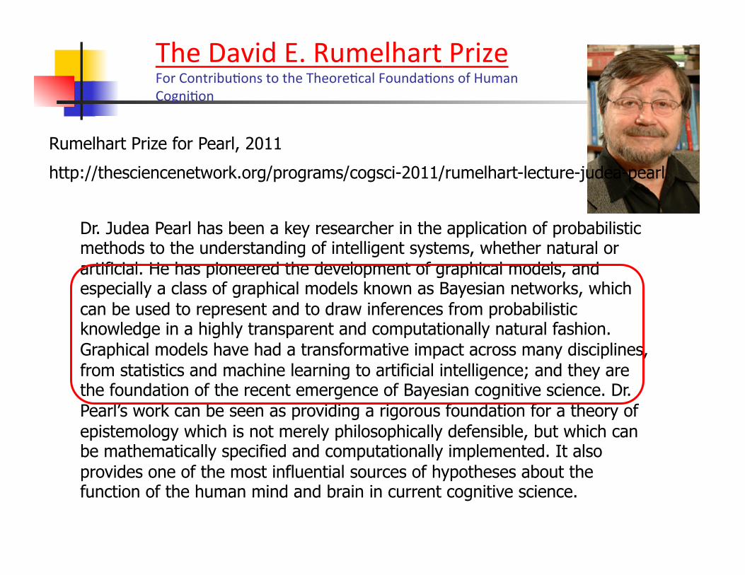
Rumelhart (1976) Figure 10

Rumelhart’s  Proposed  SoluKon  

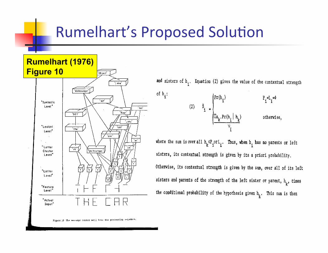
Pearl  1982:  Reverend  Bayes  on  Inference  Engines  

Bayes Net (1985)

Outline  n  Bayesian  networks  from  historical  perspecKve    n  Bayesian  networks,  a  short  tutorial    n  The    belief  propagaKon  on  trees  n  From  trees  to  graphs  n  From  Bayesian  networks  to  graphical  models  n  Some  observaKons  on  loopy  belief  propagaKon  

Outline  n  Bayesian  networks  from  historical  perspecKve    n  Bayesian  networks,  a  short  tutorial    n  The    belief  propagaKon  on  trees  n  From  trees  to  graphs  n  From  Bayesian  networks  to  graphical  models  n  Some  observaKons  on  loopy  belief  propagaKon  

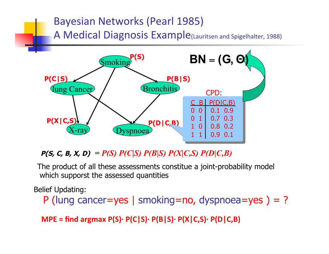
Bayesian  Networks  (Pearl  1985)  A  Medical  Diagnosis  Example(Lauritsen  and  Spigelhalter,  1988)  

lung Cancer

Smoking

X-ray

Bronchitis

Dyspnoea P(D|C,B)

P(B|S)

P(S)

P(X|C,S)

P(C|S)

P(S, C, B, X, D) = P(S) P(C|S) P(B|S) P(X|C,S) P(D|C,B) The product of all these assessments constitue a joint-probability model which supporst the assessed quantities

CPD: C B P(D|C,B) 0 0 0.1 0.9 0 1 0.7 0.3 1 0 0.8 0.2 1 1 0.9 0.1

Θ) (G,BN =

Belief Updating: P (lung cancer=yes | smoking=no, dyspnoea=yes ) = ?        MPE  =  find  argmax  P(S)·∙  P(C|S)·∙  P(B|S)·∙  P(X|C,S)·∙  P(D|C,B)  

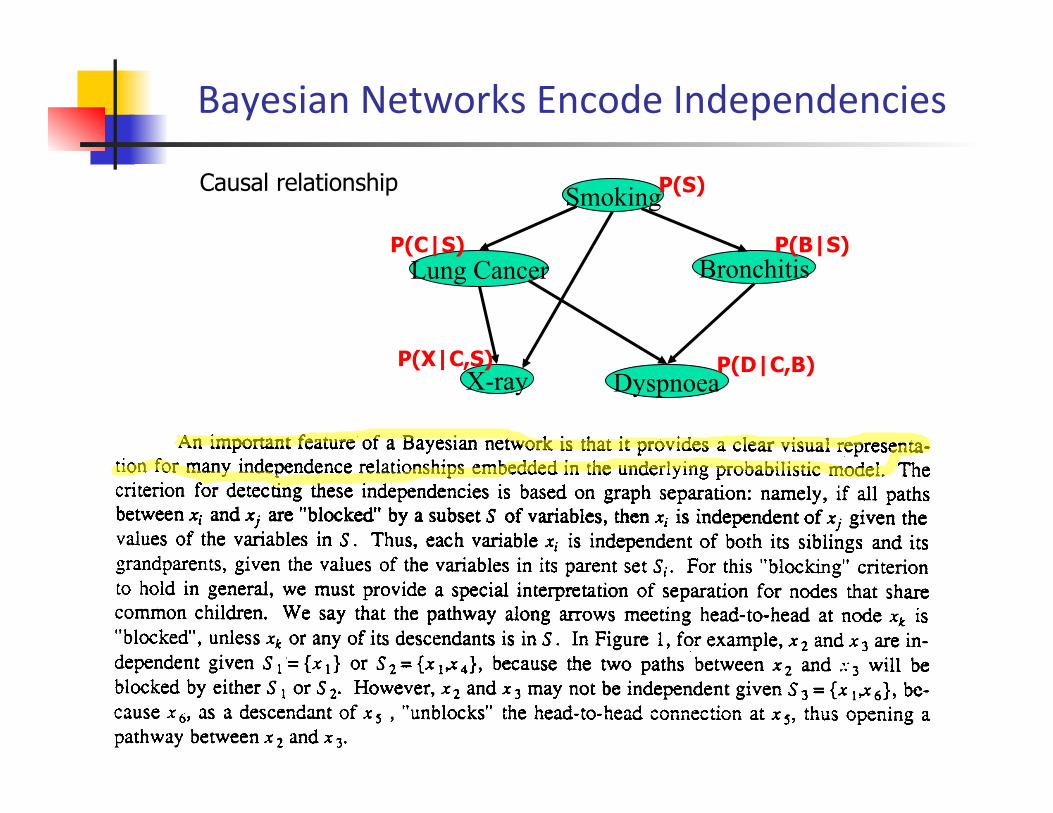
 Bayesian  Networks  Encode  Independencies    

P(S, C, B, X, D) = P(S) P(C|S) P(B|S) P(X|C,S) P(D|C,B)

Lung Cancer

Smoking

X-ray

Bronchitis

Dyspnoea P(D|C,B)

P(B|S)

P(S)

P(X|C,S)

P(C|S)

Causal relationship

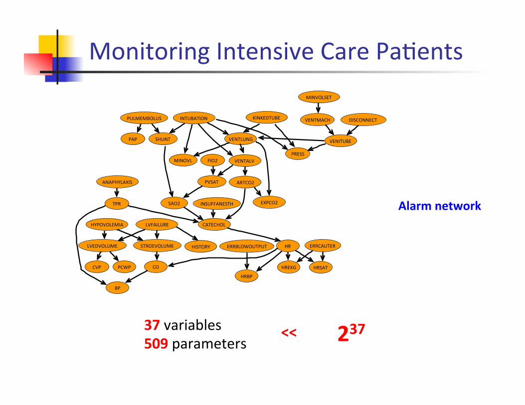
Monitoring  Intensive  Care  PaKents  

Alarm  network  

PCWP   CO  

HRBP  

HREKG   HRSAT  

ERRCAUTER  HR  HISTORY  

CATECHOL  

SAO2   EXPCO2  

ARTCO2  

VENTALV  

VENTLUNG   VENITUBE  

DISCONNECT  

MINVOLSET  

VENTMACH  KINKEDTUBE  INTUBATION  PULMEMBOLUS  

PAP   SHUNT  

ANAPHYLAXIS  

MINOVL  

PVSAT  

FIO2  PRESS  

INSUFFANESTH  TPR  

LVFAILURE  

ERRBLOWOUTPUT  STROEVOLUME  LVEDVOLUME  

HYPOVOLEMIA  

CVP  

BP  

37  variables  509  parameters   237  <<  

Outline  n  Bayesian  networks  from  historical  perspecKve  n  Bayesian  Networks  n  Belief  propagaKon  on  trees  n  From  trees  to  graphs  n  From  Bayesian  network  to  graphical  models  n  Some  observaKons  on  loopy  belief  propagaKon  

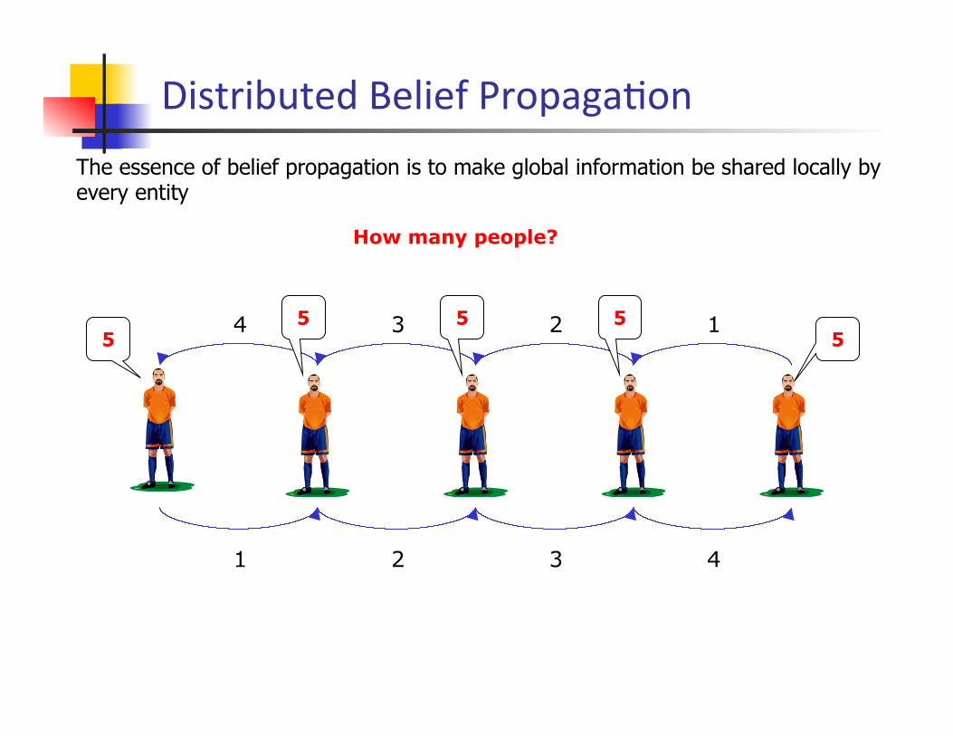
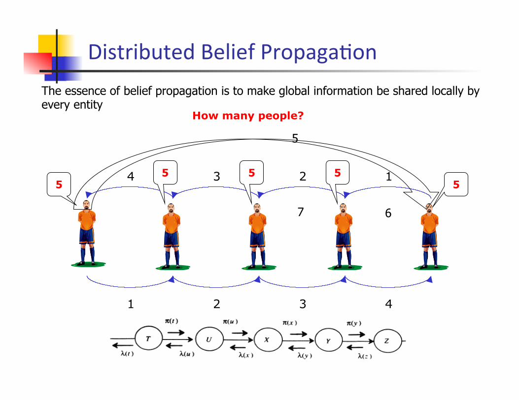
Distributed  Belief  PropagaKon  

1 2 3 4

4 3 2 1 5 5

5 5 5

How many people?

The essence of belief propagation is to make global information be shared locally by every entity

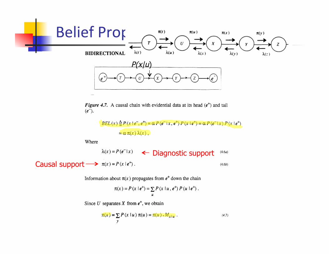
Belief  PropagaKon  on  Chains  

P(x|u)

Causal support Diagnostic support

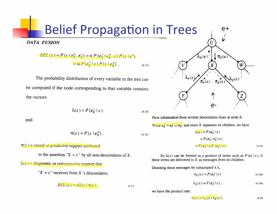
Belief  PropagaKon  in  Trees   e+

e-

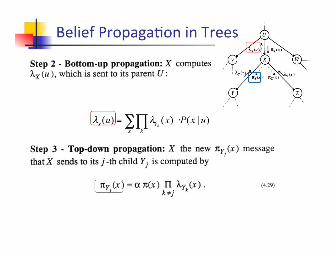
Belief  PropagaKon  in  Trees  

)|()()( uxPxux k

Yx k∑∏ ⋅= λλ

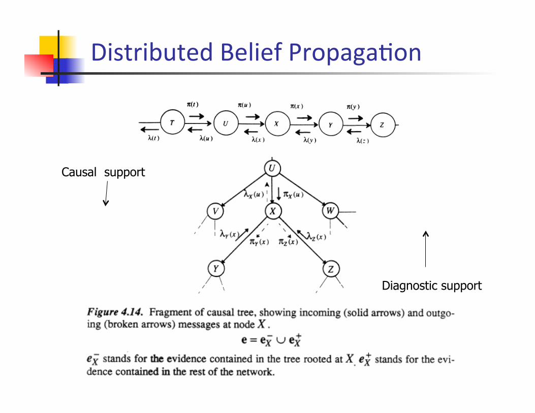
Distributed  Belief  PropagaKon  

Causal support

Diagnostic support

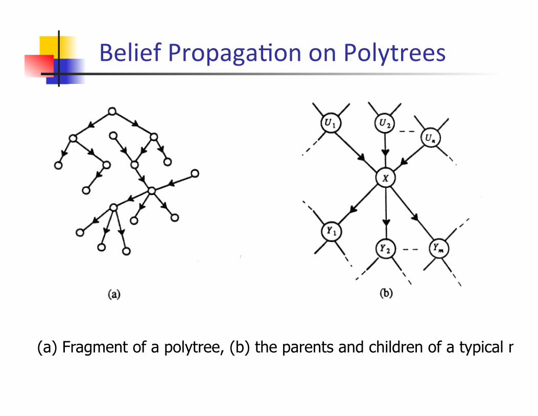
Belief  PropagaKon  on  Polytrees  

(a) Fragment of a polytree, (b) the parents and children of a typical node X

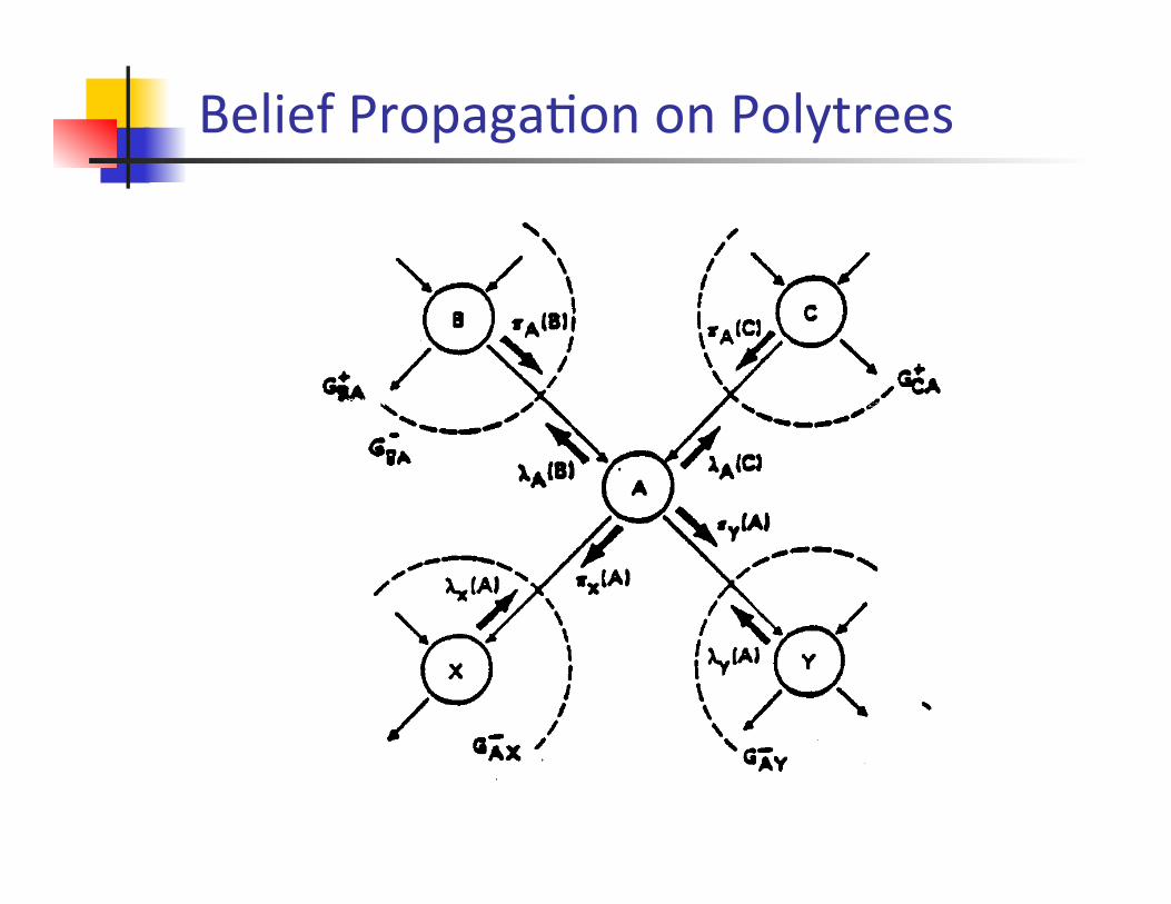
Belief  PropagaKon  on  Polytrees  

Outline  n  Bayesian  networks  from  historical  perspecKve  n  Bayesian  networks  n  Belief  propagaKon  on  trees  n  From  trees  to  graphs  n  From  Bayesian  network  to  graphical  models  n  Some  observaKon  on  loopy  belief  propagaKon  

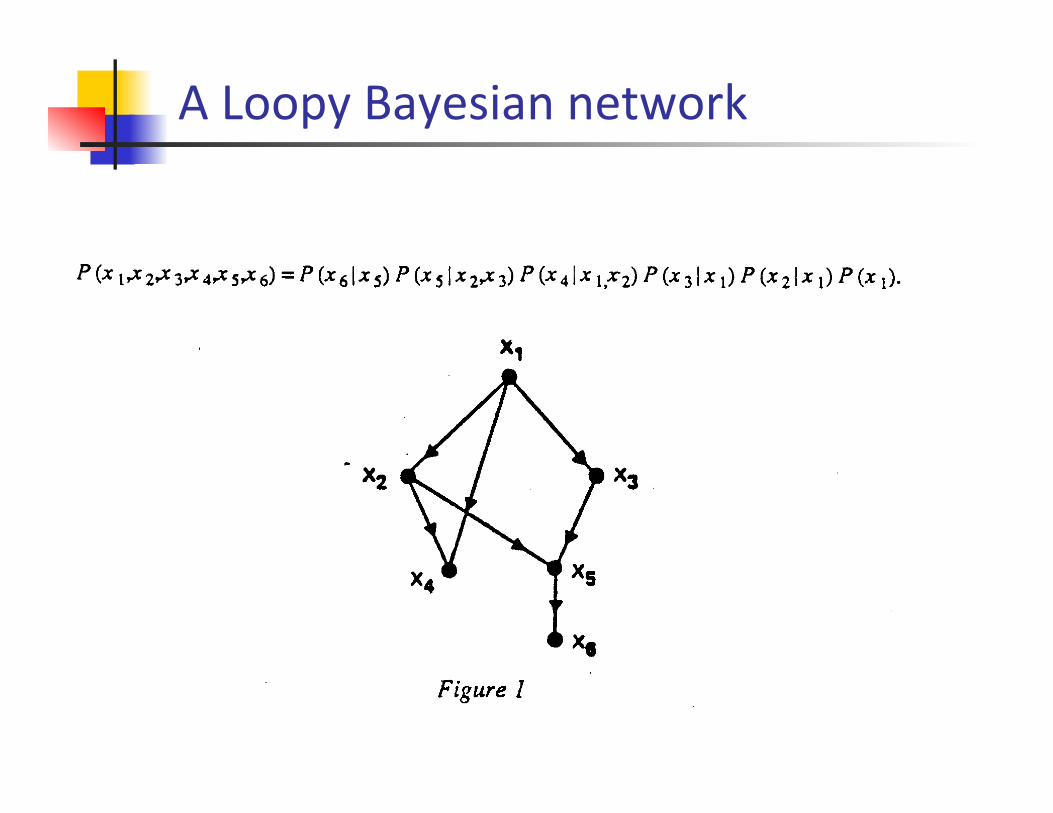
A  Loopy  Bayesian  network  

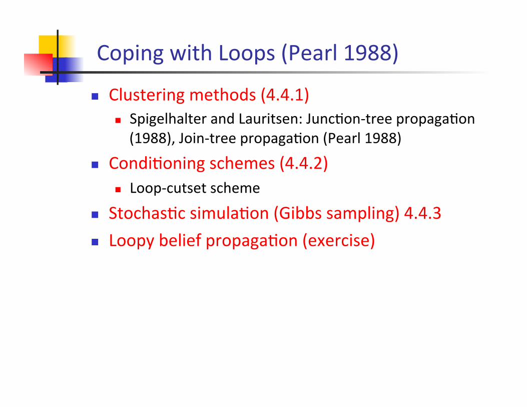
Coping  with  Loops  (Pearl  1988)  

n  Clustering  methods  (4.4.1)  n  Spigelhalter  and  Lauritsen:  JuncKon-­‐tree  propagaKon  (1988),  Join-­‐tree  propagaKon  (Pearl  1988)  

n  CondiKoning  schemes  (4.4.2)  n  Loop-­‐cutset  scheme  

n  StochasKc  simulaKon  (Gibbs  sampling)  4.4.3  n  Loopy  belief  propagaKon  (exercise)  

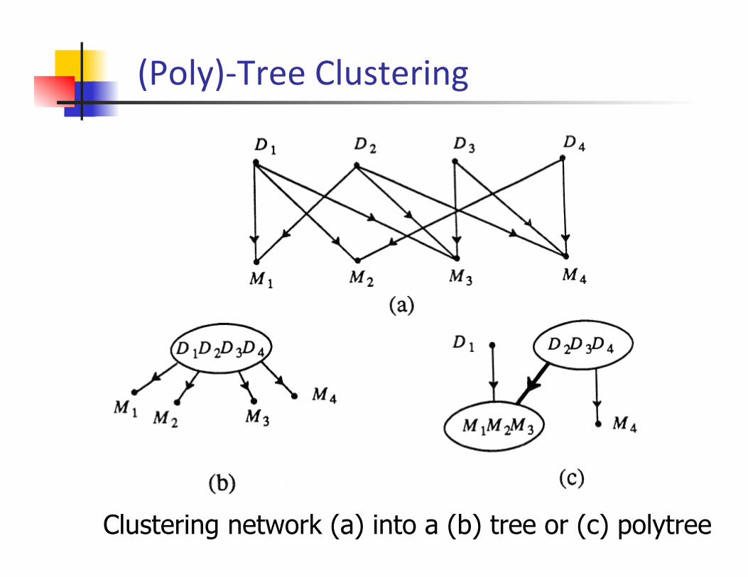
(Poly)-­‐Tree  Clustering  

Clustering network (a) into a (b) tree or (c) polytree

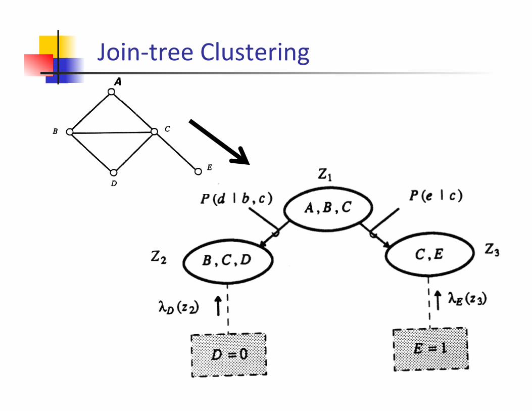
Join-­‐tree  Clustering  A

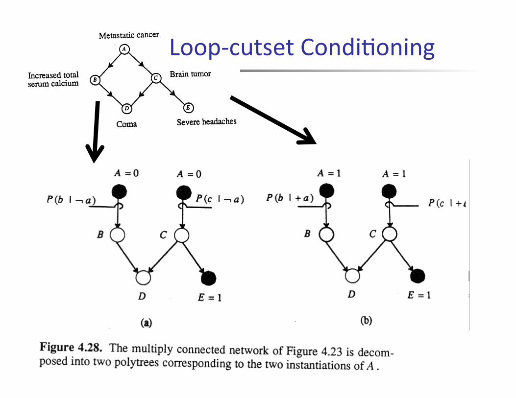
Loop-­‐cutset  CondiKoning  

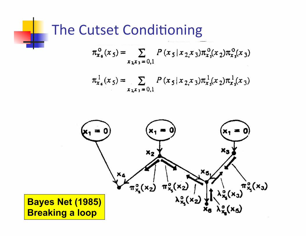
Bayes Net (1985) Breaking a loop

The  Cutset  CondiKoning  

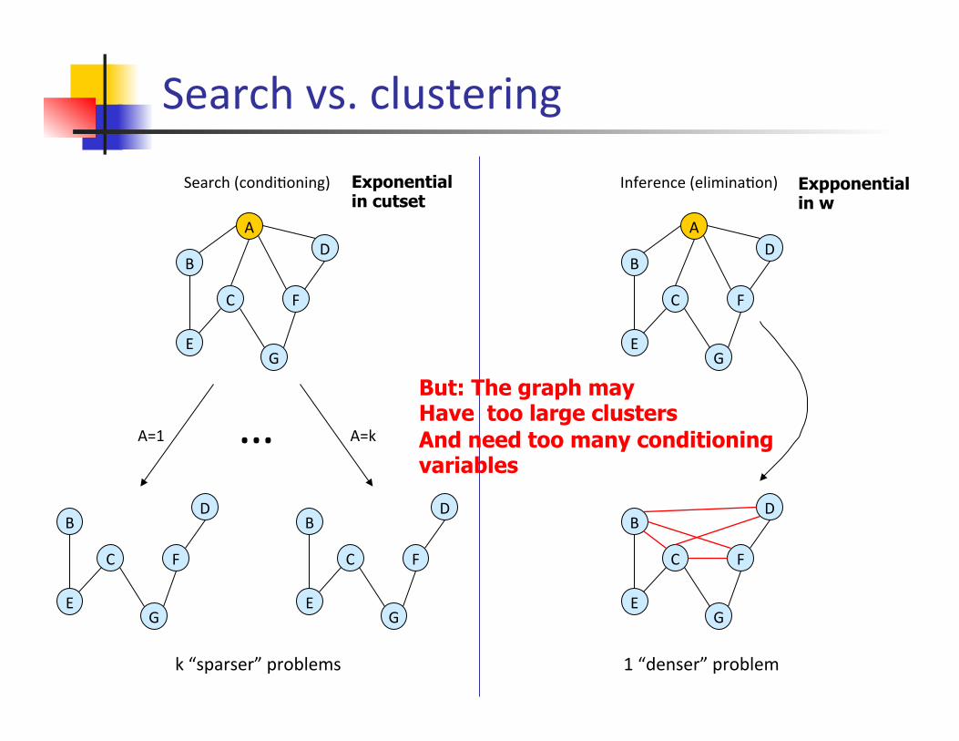
Search  vs.  clustering  

A  

G  

B  

C  

E  

D  

F  

Search  (condiKoning)       Inference  (eliminaKon)  

A=1   A=k  …  

G  

B  

C  

E  

D  

F  

G  

B  

C  

E  

D  

F  

A  

G  

B  

C  

E  

D  

F  

G  

B  

C  

E  

D  

F  

k  “sparser”  problems     1  “denser”  problem  

But: The graph may Have too large clusters And need too many conditioning variables

Expponential in w

Exponential in cutset

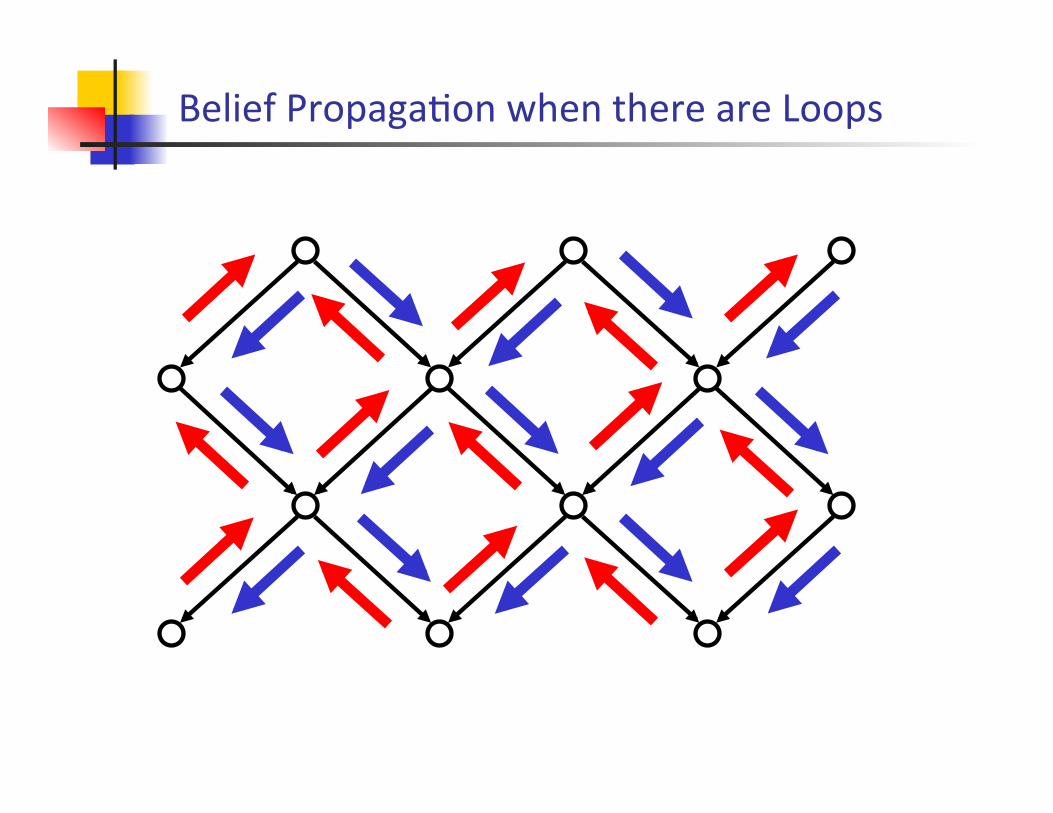
Belief  PropagaKon  when  there  are  Loops  

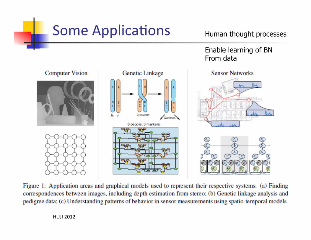
Some  ApplicaKons    

HUJI  2012  

Human thought processes

Enable learning of BN From data

Outline  n  Bayesian  networks  from  historical  perspecKve  n  Bayesian  Networks  n  Belief  propagaKon  on  trees  n  From  trees  to  graphs  n  From  Bayesian  network  to  graphical  models;  general  exact  and  approximate  algorithms  

n  Some  observaKon  on  loopy  belief  propagaKon  

33

A  B  red  green    red  yellow    green  red    green  yellow    yellow  green    yellow    red    

     

Map  coloring    

   Variables:  countries  (A  B  C  etc.)    

   Values:    colors  (red  green  blue)    

   Constraints:       ... , ED D, AB,A ≠≠≠

C  

A  

B  

D  E  

F  G  

Constraint  Networks    

Constraint  graph  

A  

B  D  

C  G  

F  

E  

34

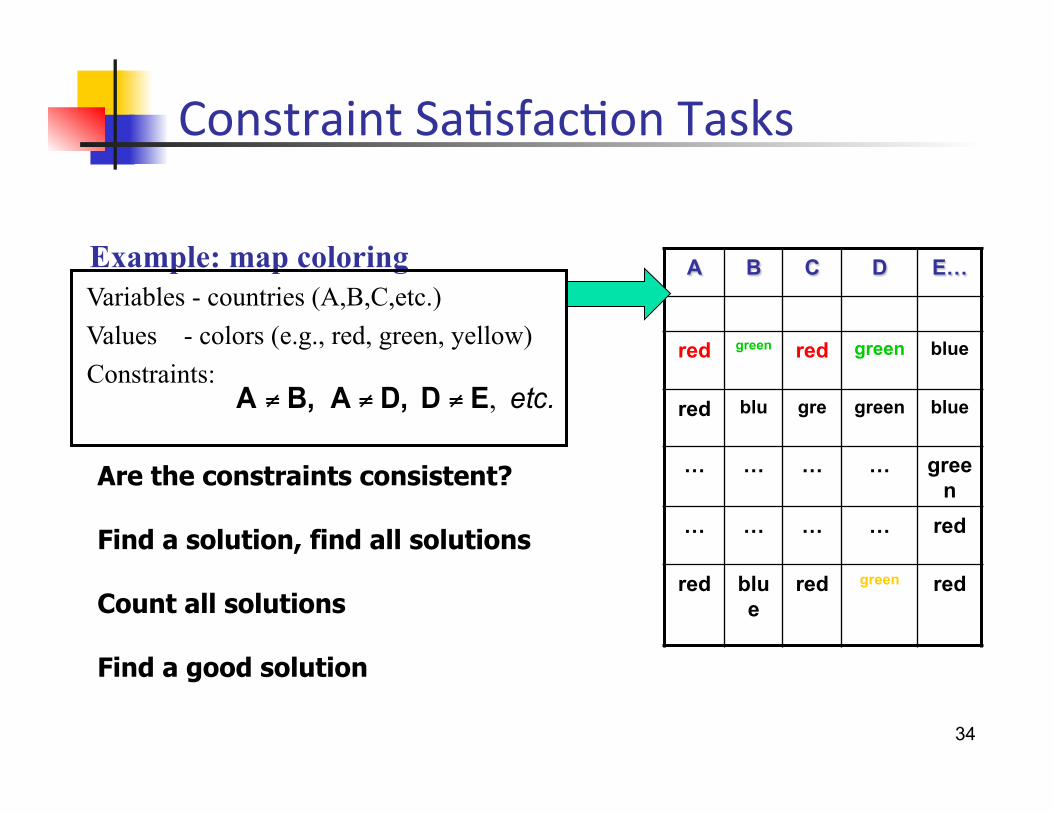
Example: map coloring Variables - countries (A,B,C,etc.) Values - colors (e.g., red, green, yellow) Constraints:

etc. ,ED D, AB,A ≠≠≠

A B C D E…

red green red green blue

red blu gre green blue

… … … … green

… … … … red

red blue

red green red

Constraint  SaKsfacKon  Tasks                              

Are the constraints consistent? Find a solution, find all solutions Count all solutions Find a good solution

A

B C

D F

G

A

B C

D F

G

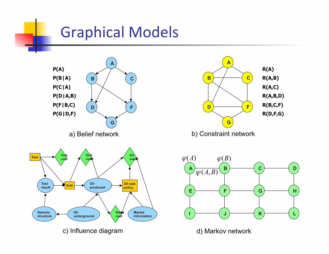
a) Belief network b) Constraint network

c) Influence diagram d) Markov network

P(A)

P(B|A)

P(C|A)

P(D|A,B)

P(F|B,C)

P(G|D,F)

R(A)

R(A,B)

R(A,C)

R(A,B,D)

R(B,C,F)

R(D,F,G)

Test

Drill Oil sale policy

Test result

Seismic structure

Oil underground

Oil produced

Test cost

Drill cost

Sales cost

Oil sales

Market information

Graphical  Models  

A B C D

E F G H

I J K L

)(Aϕ )(Bϕ

),( BAψ

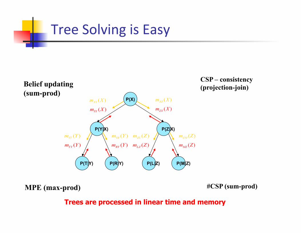
Tree  Solving  is  Easy  

Belief updating (sum-prod)

MPE (max-prod)

CSP – consistency (projection-join)

#CSP (sum-prod)

P(X)

P(Y|X) P(Z|X)

P(T|Y) P(R|Y) P(L|Z) P(M|Z)

)(XmZX

)(XmXZ

)(ZmZM)(ZmZL)(ZmMZ)(ZmLZ

)(XmYX

)(XmXY

)(YmTY

)(YmYT)(YmRY

)(YmYR

Trees are processed in linear time and memory

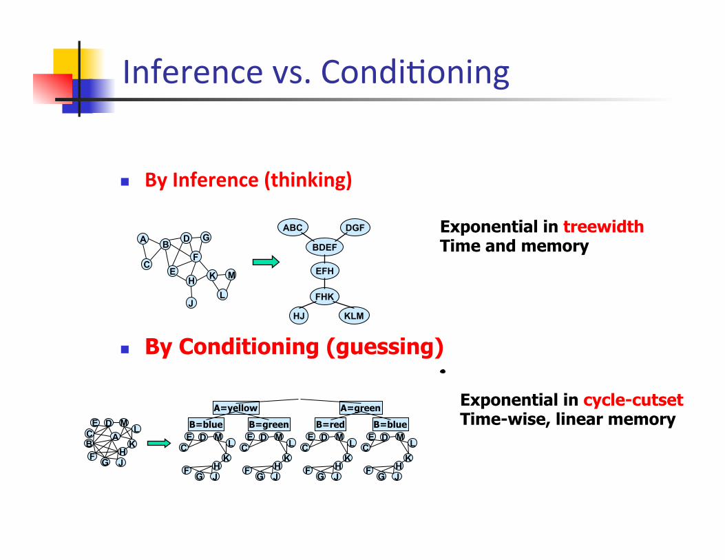
Inference  vs.  CondiKoning    

n  By  Inference  (thinking)  

E K

F

L H

C

B A

M

G

J

D ABC

BDEF

DGF

EFH

FHK

HJ KLM

n  By Conditioning (guessing)

Exponential in treewidth Time and memory

Exponential in cycle-cutset Time-wise, linear memory

A=yellow A=green

B=blue B=red B=blue B=green

C K

G

L D

F H

M

J

E A C B K

G

L D

F H

M

J

E

C K

G

L D

F H

M

J

E C

K

G

L D

F H

M

J

E C

K

G

L D

F H

M

J

E

Outline  n  Bayesian  networks  from  historical  perspecKve  n  Bayesian  Networks  n  Belief  propagaKon  on  trees  n  From  trees  to  graphs  n  From  Bayesian  network  to  graphical  models  n  Some  observaKons  on  loopy  belief  propagaKon  

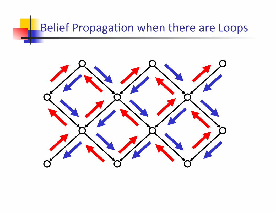
Belief  PropagaKon  when  there  are  Loops  

Distributed  Belief  PropagaKon  

1 2 3 4

4 3 2 1 5 5

5 5 5

How many people?

The essence of belief propagation is to make global information be shared locally by every entity

5

6 7

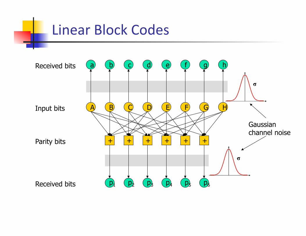
Linear  Block  Codes  

A B C D E F G H

+ + + + + +

a b c d e f g h

p1 p2 p3 p4 p5 p6

Input bits

Parity bits

Received bits

Received bits

Gaussian channel noise

σ

σ

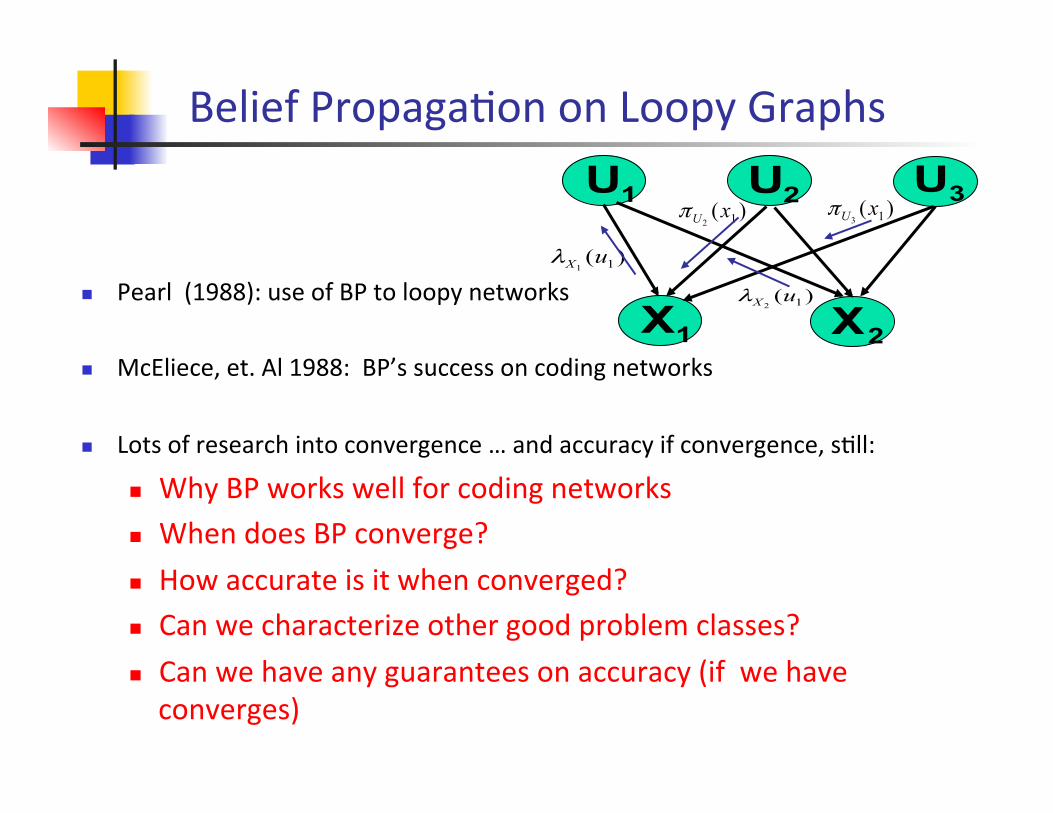
Belief  PropagaKon  on  Loopy  Graphs  

n  Pearl    (1988):  use  of  BP  to  loopy  networks  

n  McEliece,  et.  Al  1988:    BP’s  success  on  coding  networks      

n  Lots  of  research  into  convergence  …  and  accuracy  if  convergence,  sKll:  

n  Why  BP  works  well  for  coding  networks  n  When  does  BP  converge?  n  How  accurate  is  it  when  converged?  n  Can  we  characterize  other  good  problem  classes?    n  Can  we  have  any  guarantees  on  accuracy  (if    we  have  converges)  

)( 11uXλ

1U 2U 3U

2X1X

)( 12xUπ

)( 12uXλ

)( 13xUπ

3 2, 1,

3 2, 1, 3 2, 1,

1 ≤ X, Y, Z, T ≤ 3 X < Y Y = Z T < Z X ≤ T

X Y

T Z

3 2, 1, <

=

<

∧

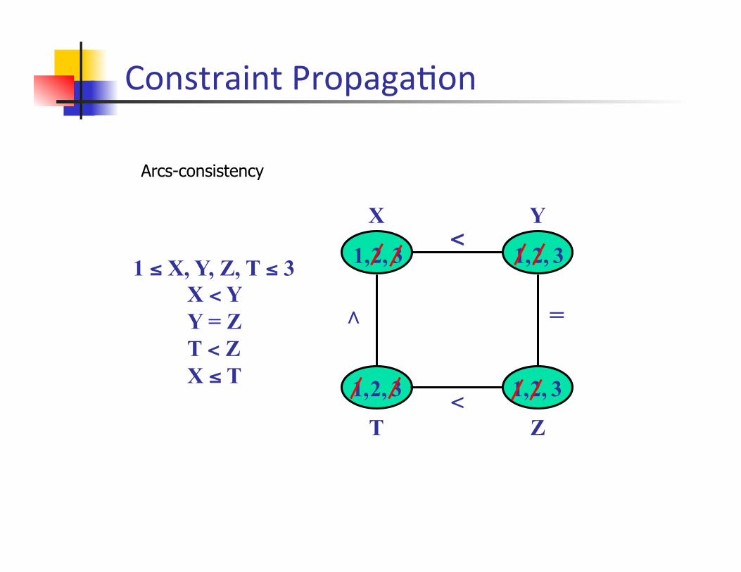
Constraint  PropagaKon    

Arcs-consistency

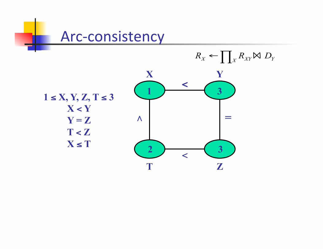
1 ≤ X, Y, Z, T ≤ 3 X < Y Y = Z T < Z X ≤ T

X Y

T Z

<

=

<

∧

1 3

2 3

∏←X YXYX DRR

Arc-­‐consistency  

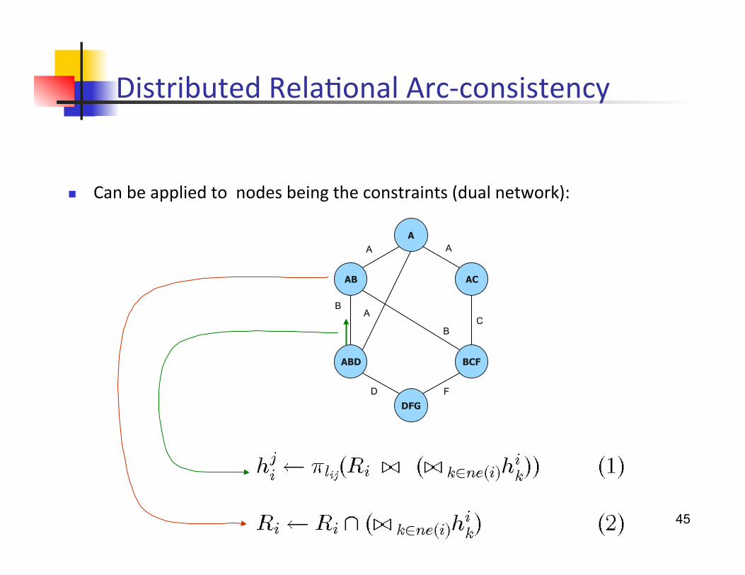
Distributed  RelaKonal  Arc-­‐consistency    

n  Can  be  applied  to    nodes  being  the  constraints  (dual  network):  

SP2 45

A

AB AC

ABD BCF

DFG

A

B

A

A

B C

D F

A

AB AC

ABD BCF

DFG

B

4 5

3

6

2

B

D F

A

A

A

C

1

A P(A) 1 .2 2 .5 3 .3 … 0

A B P(B|A) 1 2 .3 1 3 .7 2 1 .4 2 3 .6 3 1 .1 3 2 .9 … … 0

A B D P(D|A,B) 1 2 3 1 1 3 2 1 2 1 3 1 2 3 1 1 3 1 2 1 3 2 1 1 … … … 0 D F G P(G|D,F)

1 2 3 1 2 1 3 1 … … … 0

B C F P(F|B,C) 1 2 3 1 3 2 1 1 … … … 0

A C P(C|A) 1 2 1 3 2 1 … … 0

A 1 2 3

A B 1 2 1 3 2 1 2 3 3 1 3 2

A B D 1 2 3 1 3 2 2 1 3 2 3 1 3 1 2 3 2 1

D F G 1 2 3 2 1 3

B C F 1 2 3 3 2 1

A C 1 2 3 2 A

AB AC

ABD BCF

DFG

B

4 5

3

6

2

B

D F

A

A

A

C

1

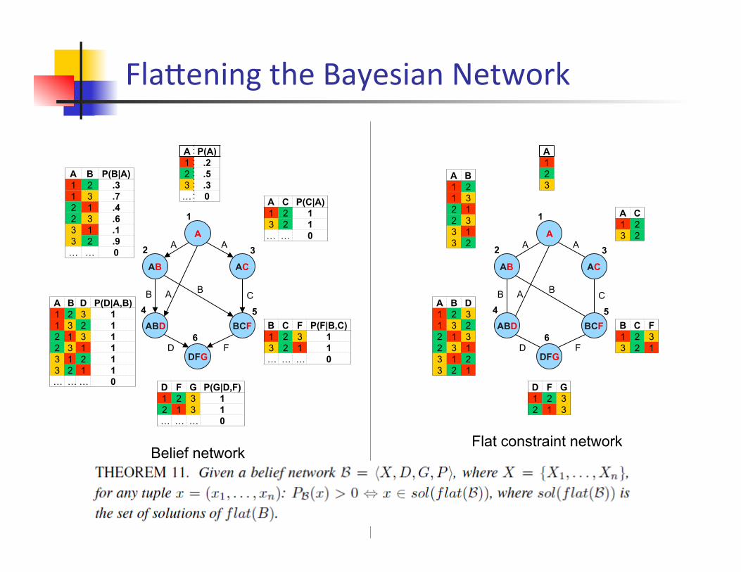
Belief network Flat constraint network

Flajening  the  Bayesian  Network  

∑ ∏∈

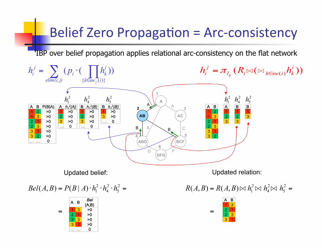
⋅=j)elim(i, inek

iki

ji

j

hph ))(()}({

)) ( ( )(ikinekil

ji hRh

ij ∈=π

A B P(B|A) 1 2 >0 1 3 >0 2 1 >0 2 3 >0 3 1 >0 3 2 >0 … … 0

A B 1 2 1 3 2 1 2 3 3 1 3 2

A h12(A)

1 >0 2 >0 3 >0 … 0

21h

24h

25h

B h12(B)

1 >0 2 >0 3 >0 … 0

B h12(B)

1 >0 3 >0 … 0

A1 2 3

21h

24h

25h

B1 2 3

B1 3

Updated belief: Updated relation:

=

=⋅⋅⋅= 25

24

21)|(),( hhhABPBABel

=

== 25

24

21 ),(),( hhhBARBAR

A B Bel (A,B)

1 3 >0 2 1 >0 2 3 >0 3 1 >0 … … 0

A B 1 3 2 1 2 3 3 1

A

AB AC

ABD BCF

DFG

B

4 5

3

6

2

B

D F

A

A

A

C

1

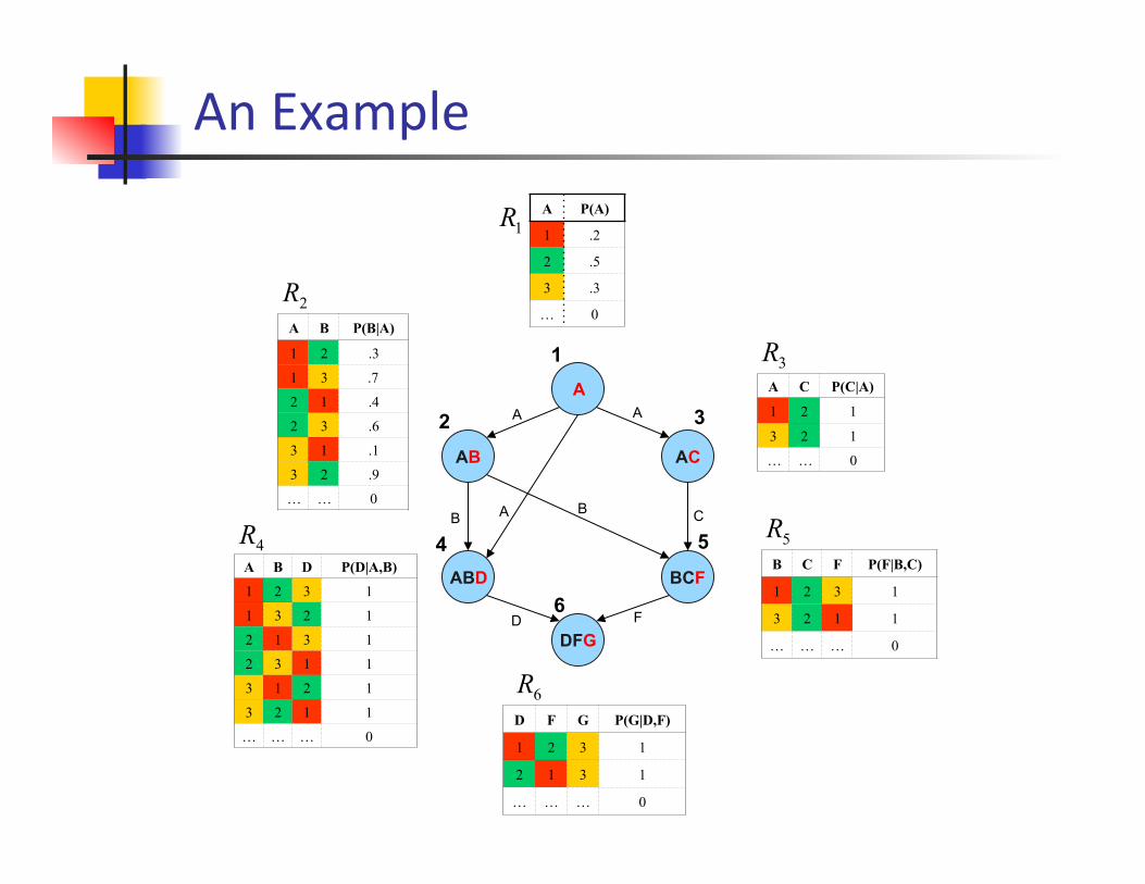
Belief  Zero  PropagaKon  =  Arc-­‐consistency  IBP over belief propagation applies relational arc-consistency on the flat network

A P(A)

1 .2

2 .5

3 .3

… 0

A C P(C|A)

1 2 1

3 2 1

… … 0

A B P(B|A)

1 2 .3

1 3 .7

2 1 .4

2 3 .6

3 1 .1

3 2 .9

… … 0

B C F P(F|B,C)

1 2 3 1

3 2 1 1

… … … 0

A B D P(D|A,B)

1 2 3 1

1 3 2 1

2 1 3 1

2 3 1 1

3 1 2 1

3 2 1 1

… … … 0 D F G P(G|D,F)

1 2 3 1

2 1 3 1

… … … 0

1R

2R

4R

3R

5R

6R

A

AB AC

ABD BCF

DFG

B

4 5

3

6

2

B

D F

A

A

A

C

1

An  Example  

A P(A)

1 >0

3 >0

… 0

A C P(C|A)

1 2 1

3 2 1

… … 0

A B P(B|A)

1 3 1

2 1 >0

2 3 >0

3 1 1

… … 0

B C F P(F|B,C)

1 2 3 1

3 2 1 1

… … … 0

A B D P(D|A,B)

1 3 2 1

2 3 1 1

3 1 2 1

3 2 1 1

… … … 0

D F G P(G|D,F)

2 1 3 1

… … … 0

2R

4R

3R

5R

6R

A

AB AC

ABD BCF

DFG

B

4 5

3

6

2

B

D F

A

A

A

C

1

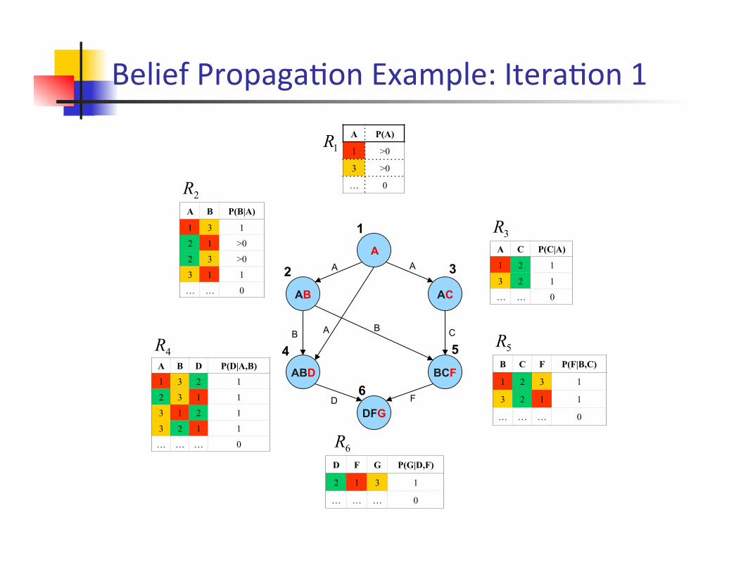
Belief  PropagaKon  Example:  IteraKon  1  

1R

A P(A)

1 >0

3 >0

… 0

A C P(C|A)

1 2 1

3 2 1

… … 0

A B P(B|A)

1 3 1

3 1 1

… … 0

B C F P(F|B,C)

3 2 1 1

… … … 0

A B D P(D|A,B)

1 3 2 1

3 1 2 1

… … … 0

D F G P(G|D,F)

2 1 3 1

… … … 0

2R

4R

3R

5R

6R

A

AB AC

ABD BCF

DFG

B

4 5

3

6

2

B

D F

A

A

A

C

1

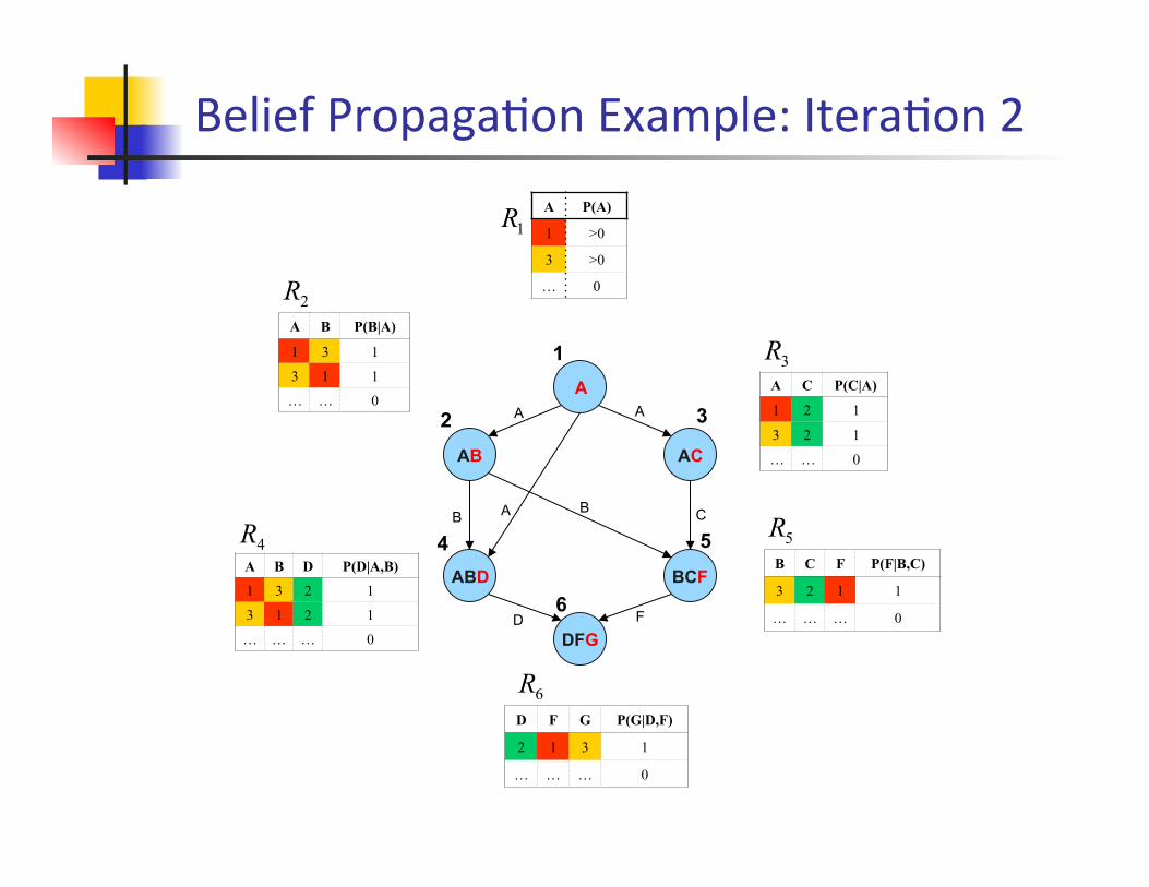
Belief  PropagaKon  Example:  IteraKon  2  

1R

A P(A)

1 >0

3 >0

… 0

A C P(C|A)

1 2 1

3 2 1

… … 0

A B P(B|A)

1 3 1 … … 0

B C F P(F|B,C)

3 2 1 1

… … … 0

A B D P(D|A,B)

1 3 2 1

3 1 2 1

… … … 0

D F G P(G|D,F)

2 1 3 1

… … … 0

2R

4R

3R

5R

6R

A

AB AC

ABD BCF

DFG

B

4 5

3

6

2

B

D F

A

A

A

C

1

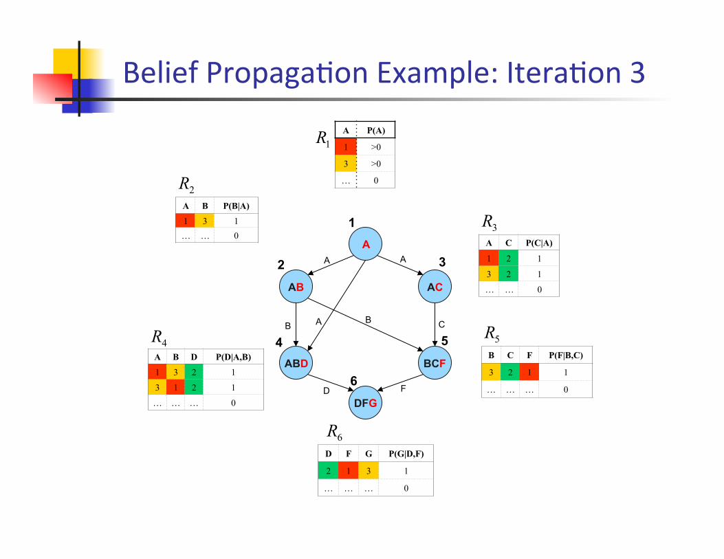
Belief  PropagaKon  Example:  IteraKon  3  

1R

A P(A)

1 1

… 0

A C P(C|A)

1 2 1

3 2 1

… … 0

A B P(B|A)

1 3 1

… … 0

B C F P(F|B,C)

3 2 1 1

… … … 0

A B D P(D|A,B)

1 3 2 1

… … … 0

D F G P(G|D,F)

2 1 3 1

… … … 0

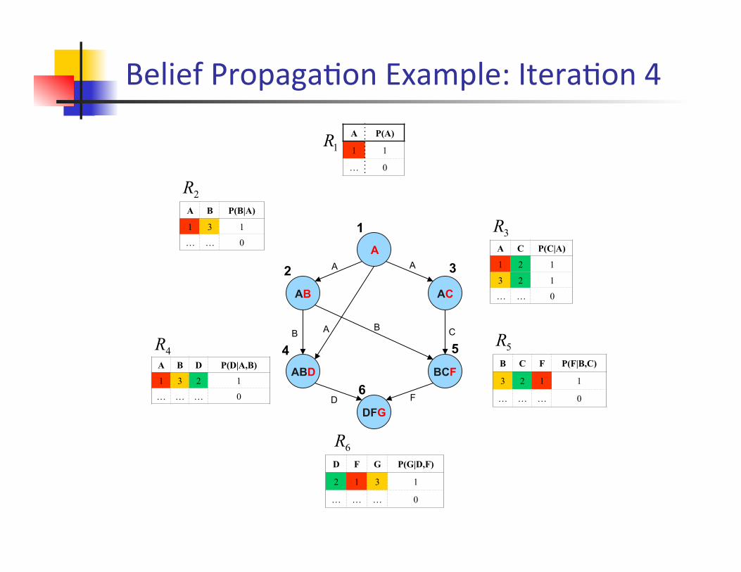
Belief  PropagaKon  Example:  IteraKon  4  

2R

4R

3R

5R

6R

A

AB AC

ABD BCF

DFG

B

4 5

3

6

2

B

D F

A

A

A

C

1

1R

A P(A)

1 1

… 0

A C P(C|A)

1 2 1

… … 0

A B P(B|A)

1 3 1

… … 0

B C F P(F|B,C)

3 2 1 1

… … … 0

A B D P(D|A,B)

1 3 2 1

… … … 0

D F G P(G|D,F)

2 1 3 1

… … … 0

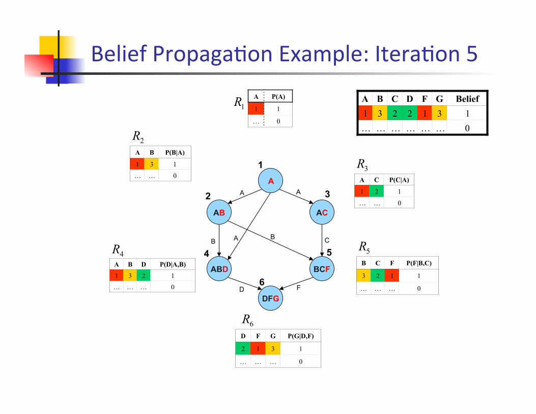
A B C D F G Belief 1 3 2 2 1 3 1 … … … … … … 0

Belief  PropagaKon  Example:  IteraKon  5  

2R

4R

3R

5R

6R

A

AB AC

ABD BCF

DFG

B

4 5

3

6

2

B

D F

A

A

A

C

1

1R

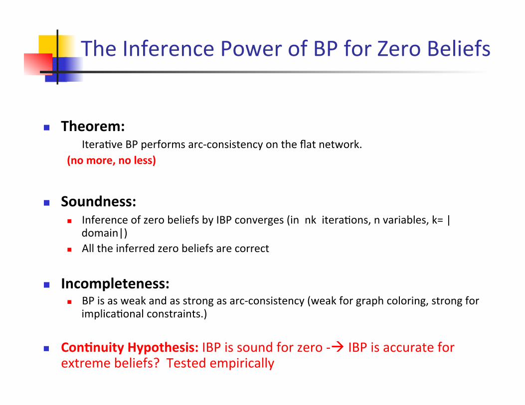
The  Inference  Power  of  BP  for  Zero  Beliefs  

n  Theorem:          IteraKve  BP  performs  arc-­‐consistency  on  the  flat  network.      

(no  more,  no  less)    

n  Soundness:        n  Inference  of  zero  beliefs  by  IBP  converges  (in    nk    iteraKons,  n  variables,  k=  |

domain|)  n  All  the  inferred  zero  beliefs  are  correct  

n  Incompleteness:        n  BP  is  as  weak  and  as  strong  as  arc-­‐consistency  (weak  for  graph  coloring,  strong  for  

implicaKonal  constraints.)  

n  Con5nuity  Hypothesis:  IBP  is  sound  for  zero  -­‐à  IBP  is  accurate  for  extreme  beliefs?    Tested  empirically  

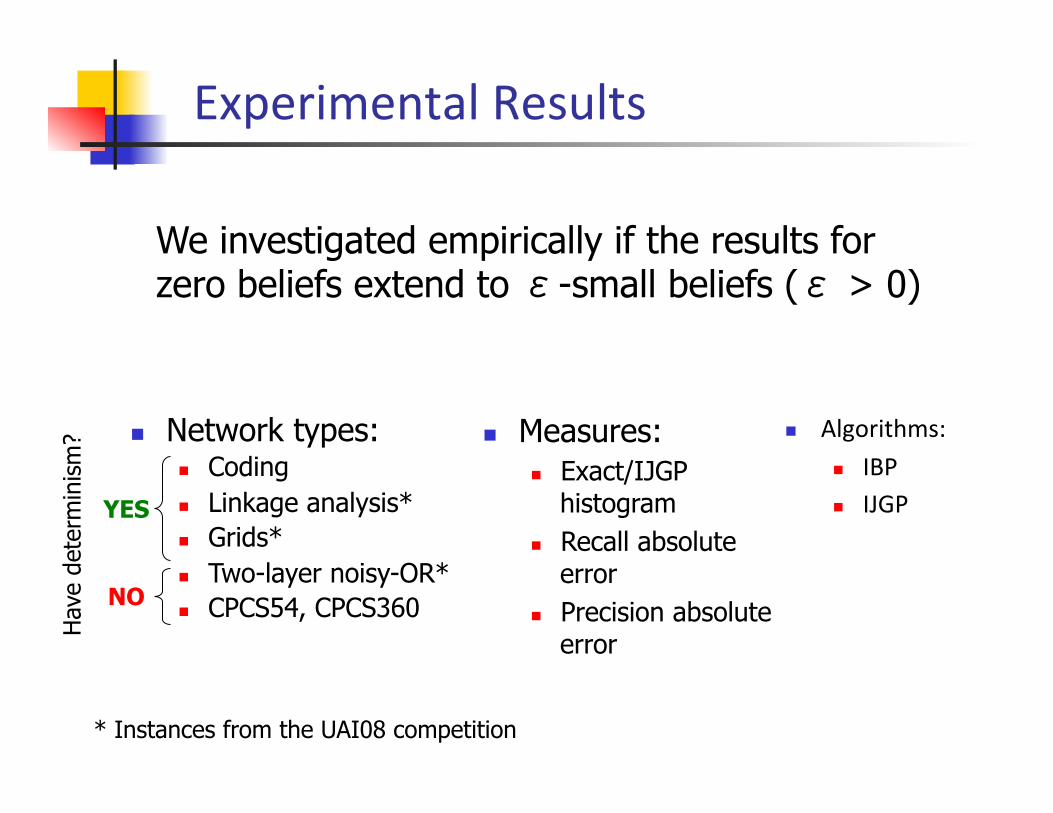
Experimental  Results  

n  Algorithms:  n  IBP  n  IJGP  

n  Measures: n  Exact/IJGP

histogram n  Recall absolute

error n  Precision absolute

error

n  Network types: n  Coding n  Linkage analysis* n  Grids* n  Two-layer noisy-OR* n  CPCS54, CPCS360

We investigated empirically if the results for zero beliefs extend to ε-small beliefs (ε > 0)

* Instances from the UAI08 competition

Hav

e de

term

inis

m?

YES

NO

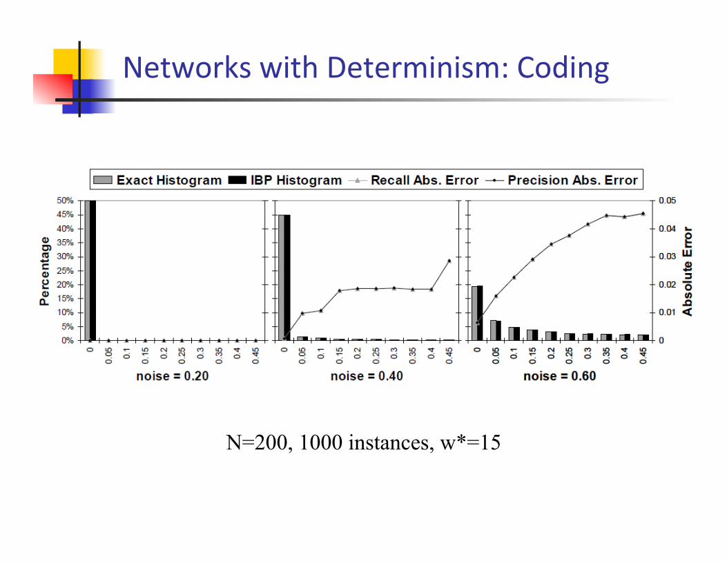
Networks  with  Determinism:  Coding  

N=200, 1000 instances, w*=15

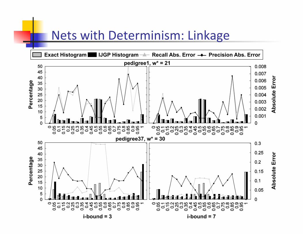
Nets  with  Determinism:  Linkage  Pe

rcen

tage

Abs

olut

e Er

ror

pedigree1, w* = 21 Exact Histogram IJGP Histogram Recall Abs. Error Precision Abs. Error

Perc

enta

ge

Abs

olut

e Er

ror

pedigree37, w* = 30

i-bound = 3 i-bound = 7

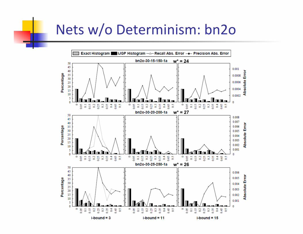
Nets  w/o  Determinism:  bn2o  

w* = 24

w* = 27

w* = 26

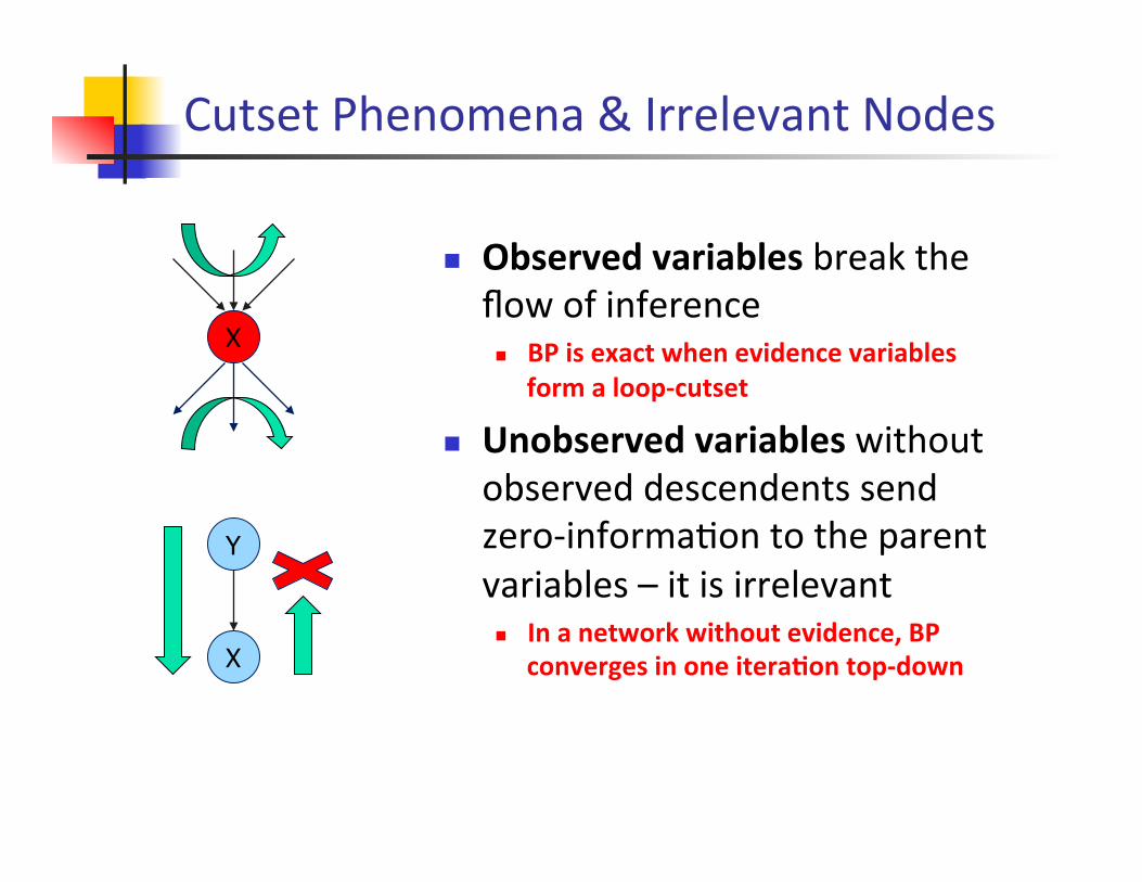
Cutset  Phenomena  &  Irrelevant  Nodes  

n  Observed  variables  break  the  flow  of  inference    n  BP  is  exact  when  evidence  variables  

form  a  loop-­‐cutset  

n  Unobserved  variables  without  observed  descendents  send  zero-­‐informaKon  to  the  parent  variables  –  it  is  irrelevant  n  In  a  network  without  evidence,  BP  

converges  in  one  itera5on  top-­‐down  

X

X

Y

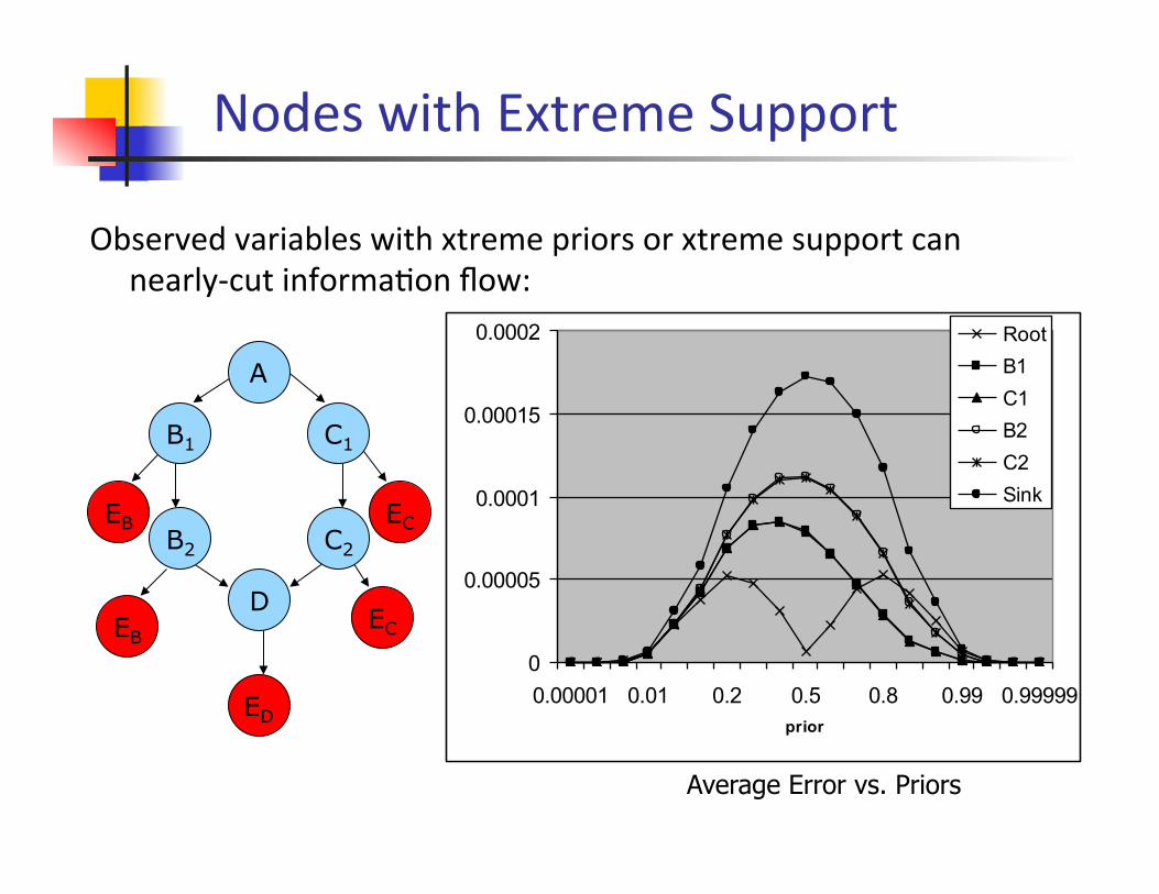
Nodes  with  Extreme  Support  

Observed  variables  with  xtreme  priors  or  xtreme  support  can  nearly-­‐cut  informaKon  flow:  

0

0.00005

0.0001

0.00015

0.0002

0.00001 0.01 0.2 0.5 0.8 0.99 0.99999prior

RootB1C1B2C2Sink

D

B1

ED

A

B2

EB EC

EB EC

C1

C2

Average Error vs. Priors

Conclusion:  Networks  with  Determinism  

BP  converges  &  sound  for  zero  beliefs  

n  IBP’s  power  to  infer  zeros  is  as  weak  or  as  strong  as  arc-­‐consistency  

n  However:  inference  of  extreme  beliefs  can  be  wrong.  

n  Cutset  property  (Bidyuk  and  Dechter,  2000):    n  Evidence  and  inferred  singleton  act  like  cutset  n  If  zeros  are  cycle-­‐cutset,  all  beliefs  are    exact  n  Extensions  to  epsilon-­‐cutset  were  supported  empirically.  

n  IJGP  is  an  anyKme  good  tradeoff  propagaKon  scheme  

Thank  You  

Rina Dechter, Bozhena Bidyuk, Robert Mateescu and Emma Rollon. "On the Power of Belief Propagation: A Constraint Propagation Perspective" in Festschrift book in honor of Judea Pearl, 2010

Heuristics, Probability and Causality, A Tribute to Judea Pearl Editors Rina Dechter, Hector Geffner and Joseph Y. Halpern http://bayes.cs.ucla.edu/TRIBUTE/pearl-tribute2010.htm http://www.ics.uci.edu/~dechter/publications.html

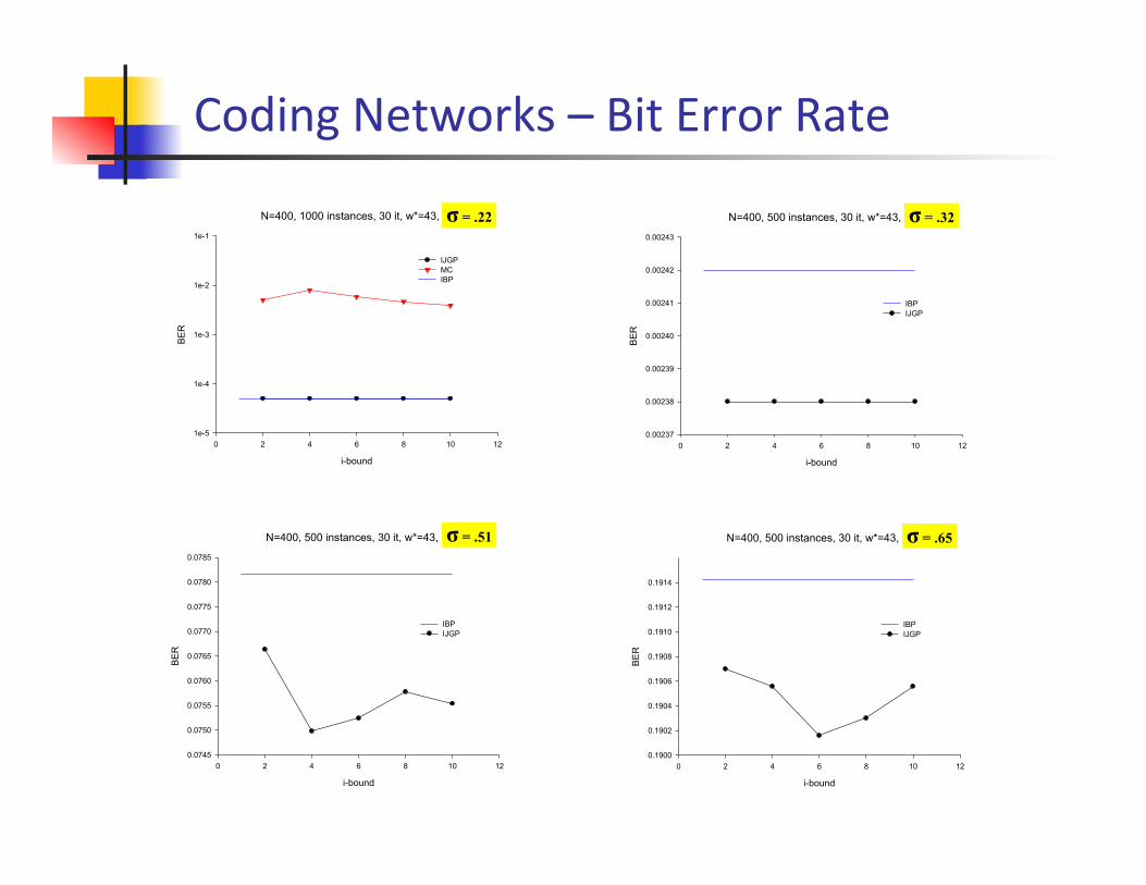
Coding  Networks  –  Bit  Error  Rate  

Coding, N=400, 500 instances, 30 it, w*=43, sigma=.32

i-bound

0 2 4 6 8 10 12

BER

0.00237

0.00238

0.00239

0.00240

0.00241

0.00242

0.00243

IBPIJGP

Coding, N=400, 500 instances, 30 it, w*=43, sigma=.51

i-bound

0 2 4 6 8 10 12

BER

0.0745

0.0750

0.0755

0.0760

0.0765

0.0770

0.0775

0.0780

0.0785

IBPIJGP

Coding, N=400, 500 instances, 30 it, w*=43, sigma=.65

i-bound

0 2 4 6 8 10 12

BER

0.1900

0.1902

0.1904

0.1906

0.1908

0.1910

0.1912

0.1914

IBPIJGP

Coding, N=400, 1000 instances, 30 it, w*=43, sigma=.22

i-bound

0 2 4 6 8 10 12

BER

1e-5

1e-4

1e-3

1e-2

1e-1

IJGPMCIBP

σ = .22

σ = .51 σ = .65

σ = .32

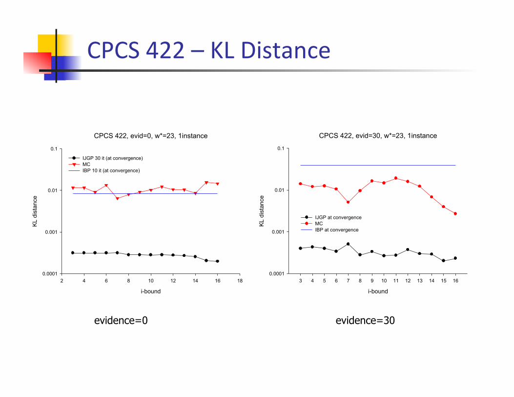
CPCS 422, evid=0, w*=23, 1instance

i-bound

2 4 6 8 10 12 14 16 18

KL d

ista

nce

0.0001

0.001

0.01

0.1

IJGP 30 it (at convergence)MCIBP 10 it (at convergence)

CPCS  422  –  KL  Distance  

CPCS 422, evid=30, w*=23, 1instance

i-bound

3 4 5 6 7 8 9 10 11 12 13 14 15 16

KL d

ista

nce

0.0001

0.001

0.01

0.1

IJGP at convergenceMCIBP at convergence

evidence=0 evidence=30

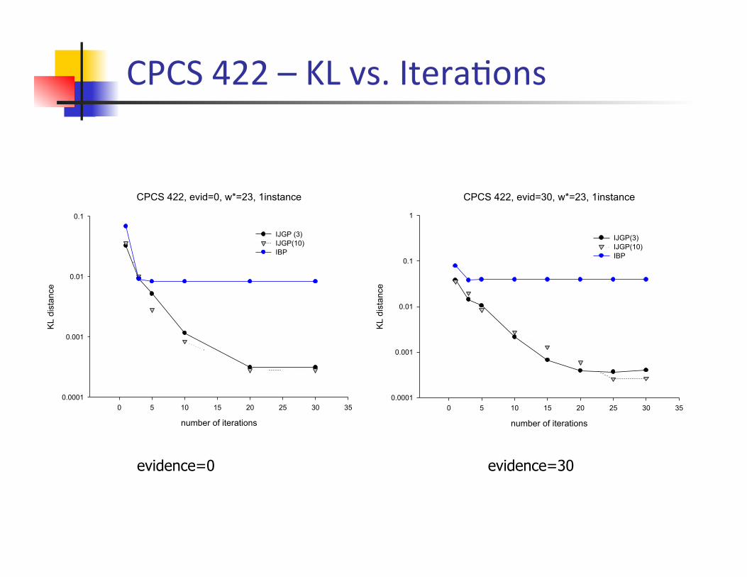
CPCS  422  –  KL  vs.  IteraKons  

CPCS 422, evid=0, w*=23, 1instance

number of iterations

0 5 10 15 20 25 30 35

KL d

ista

nce

0.0001

0.001

0.01

0.1

IJGP (3)IJGP(10)IBP

CPCS 422, evid=30, w*=23, 1instance

number of iterations

0 5 10 15 20 25 30 35

KL d

ista

nce

0.0001

0.001

0.01

0.1

1

IJGP(3)IJGP(10)IBP

evidence=0 evidence=30

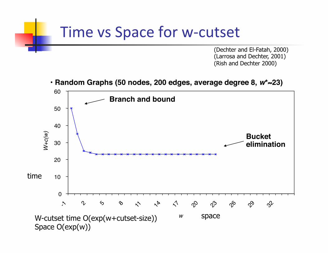
Time  vs  Space  for  w-­‐cutset  

•  Random Graphs (50 nodes, 200 edges, average degree 8, w*≈23)!

Branch and bound!

Bucket !elimination!

0

10

20

30

40

50

60

w

W+c(w)

space

time

(Dechter and El-Fatah, 2000) (Larrosa and Dechter, 2001) (Rish and Dechter 2000)

W-cutset time O(exp(w+cutset-size)) Space O(exp(w))