bcs.solano.edubcs.solano.edu/workarea/jurrutia/Coursework/CIS 23 - Data... · Web viewNote that Nx/y means the yth root of N raised to the ... The word radix means the base of a

1 CHAPTER 7 Advanced Sorting

CHAPTER 7 Advanced Sorting

IN THIS CHAPTER

• Shellsort

• Partitioning

• Quicksort

• Radix Sort

We discussed simple sorting in the aptly titled Chapter 3, “Simple Sorting.” The sorts described there—

the bubble, selection, and insertion sorts—are easy to implement but are rather slow. In Chapter 6,

“Recursion,” we described the mergesort. It runs much faster than the simple sorts but requires twice as

much space as the original array; this is often a serious drawback.

This chapter covers two advanced approaches to sorting: Shellsort and quicksort. These sorts both

operate much faster than the simple sorts: the Shellsort in about O(N*(logN)2) time, and quicksort in

O(N*logN) time. Neither of these sorts requires a large amount of extra space, as mergesort does. The

Shellsort is almost as easy to implement as mergesort, while quicksort is the fastest of all the general-

purpose sorts. We’ll conclude the chapter with a brief mention of the radix sort, an unusual and

interesting approach to sorting.

We’ll examine the Shellsort first. Quicksort is based on the idea of partitioning, so we’ll then examine

partitioning separately, before examining quicksort itself.

Shellsort

The Shellsort is named for Donald L. Shell, the computer scientist who discovered it in 1959. It’s based

on the insertion sort, but adds a new feature that dramatically improves the insertion sort’s

performance.

The Shellsort is good for medium-sized arrays, perhaps up to a few thousand items, depending on the

particular implementation. It’s not quite as fast as quicksort and other O(N*logN) sorts, so it’s not

optimum for very largefiles. However, it’s much faster than the O(N2) sorts like the selection sort and

the insertion sort, and it’s very easy to implement: The code is short and simple.

The worst-case performance is not significantly worse than the average performance. (We’ll see later in


this chapter that the worst-case performance for quicksort can be much worse unless precautions are

taken.) Some experts (see Sedgewick in Appendix B, “Further Reading”) recommend starting with a

Shellsort for almost any sorting project and changing to a more advanced sort, like quicksort, only if

Shellsort proves too slow in practice.

Insertion Sort: Too Many Copies

Because Shellsort is based on the insertion sort, you might want to review the section titled “Insertion

Sort” in Chapter 3. Recall that partway through the insertion sort the items to the left of a marker are

internally sorted (sorted among themselves) and items to the right are not. The algorithm removes the

item at the marker and stores it in a temporary variable. Then, beginning with the item to the left of

the newly vacated cell, it shifts the sorted items right one cell at a time, until the item in the temporary

variable can be reinserted in sorted order.

Here’s the problem with the insertion sort. Suppose a small item is on the far right, where the large

items should be. To move this small item to its proper place on the left, all the intervening items

(between the place where it is and where it should be) must be shifted one space right. This step takes

close to N copies, just for one item. Not all the items must be moved a full N spaces, but the average

item must be moved N/2 spaces, which takes N times N/2 shifts for a total of N2/2 copies. Thus, the

performance of insertion sort is O(N2).

This performance could be improved if we could somehow move a smaller item many spaces to the left

without shifting all the intermediate items individually.

N-Sorting

The Shellsort achieves these large shifts by insertion-sorting widely spaced elements. After they are

sorted, it sorts somewhat less widely spaced elements, and so on. The spacing between elements for

these sorts is called the increment and is traditionally represented by the letter h. Figure 7.1 shows the

first step in the process of sorting a

10-element array with an increment of 4. Here the elements 0, 4, and 8 are sorted.

After 0, 4, and 8 are sorted, the algorithm shifts over one cell and sorts 1, 5, and 9. This process

continues until all the elements have been 4-sorted, which means that all items spaced four cells apart

are sorted among themselves. The process is shown (using a more compact visual metaphor) in Figure

7.2.


After the complete 4-sort, the array can be thought of as comprising four subarrays: (0,4,8), (1,5,9),

(2,6), and (3,7), each of which is completely sorted. These subarrays are interleaved but otherwise

independent.

FIGURE 7.1 4-sorting 0, 4, and 8.

Notice that, in this particular example, at the end of the 4-sort no item is more than two cells from

where it would be if the array were completely sorted. This is what is meant by an array being “almost”

sorted and is the secret of the Shellsort. By creating interleaved, internally sorted sets of items, we

minimize the amount of work that must be done to complete the sort.

Now, as we noted in Chapter 3, the insertion sort is very efficient when operating on an array that’s

almost sorted. If it needs to move items only one or two cells to sort the file, it can operate in almost

O(N) time. Thus, after the array has been 4-sorted, we can 1-sort it using the ordinary insertion sort. The

combination of the 4-sort and the 1-sort is much faster than simply applying the ordinary insertion sort

without the preliminary 4-sort.


Diminishing Gaps

We’ve shown an initial interval—or gap—of 4 cells for sorting a 10-cell array. For larger arrays the

interval should start out much larger. The interval is then repeatedly reduced until it becomes 1.

For instance, an array of 1,000 items might be 364-sorted, then 121-sorted, then 40- sorted, then 13-

sorted, then 4-sorted, and finally 1-sorted. The sequence of numbers used to generate the intervals (in

this example, 364, 121, 40, 13, 4, 1) is called the interval sequence or gap sequence. The particular

interval sequence shown here, attributed to Knuth (see Appendix B), is a popular one. In reversed form,

starting from 1, it’s generated by the recursive expression

h = 3*h + 1

where the initial value of h is 1. The first two columns of Table 7.1 show how this formula generates the

sequence.


FIGURE 7.2 A complete 4-sort.


TABLE 7.1 Knuth’s Interval Sequence

h 3*h + 1 (h–1) / 3

1 4

4 13 1

13 40 4

40 121 13

121 364 40

364 1093 121

1093 3280 364

There are other approaches to generating the interval sequence; we’ll return to this issue later. First,

we’ll explore how the Shellsort works using Knuth’s sequence.

In the sorting algorithm, the sequence-generating formula is first used in a short loop to figure out the

initial gap. A value of 1 is used for the first value of h, and the h=h*3+1 formula is applied to generate

the sequence 1, 4, 13, 40, 121, 364, and so on. This process ends when the gap is larger than the array.

For a 1,000-element array, the seventh number in the sequence, 1,093, is too large. Thus, we begin the

sorting process with the sixth-largest number, creating a 364-sort. Then, each time through the outer

loop of the sorting routine, we reduce the interval using the inverse of the formula previously given:

h = (h–1) / 3

This is shown in the third column of Table 7.1. This inverse formula generates the reverse sequence 364,

121, 40, 13, 4, 1. Starting with 364, each of these numbers is used to n-sort the array. When the array

has been 1-sorted, the algorithm is done.

The Shellsort Workshop Applet

You can use the Shellsort Workshop applet to see how this sort works. Figure 7.3 shows the applet after

all the bars have been 4-sorted, just as the 1-sort begins.


FIGURE 7.3 The Shellsort Workshop applet.

As you single-step through the algorithm, you’ll notice that the explanation we gave in the preceding

discussion is slightly simplified. The sequence for the 4-sort is not actually (0,4,8), (1,5,9), (2,6), and (3,7).

Instead, the first two elements of each group of three are sorted first, then the first two elements of the

second group, and so on. Once the first two elements of all the groups are sorted, the algorithm returns

and sorts three-element groups. The actual sequence is (0,4), (1,5), (2,6), (3,7), (0,4,8), (1,5,9).

It might seem more obvious for the algorithm to 4-sort each complete subarray first—(0,4), (0,4,8),

(1,5), (1,5,9), (2,6), (3,7)—but the algorithm handles the array indices more efficiently using the first

scheme.

The Shellsort is actually not very efficient with only 10 items, making almost as many swaps and

comparisons as the insertion sort. However, with 64 bars the improvement becomes significant.

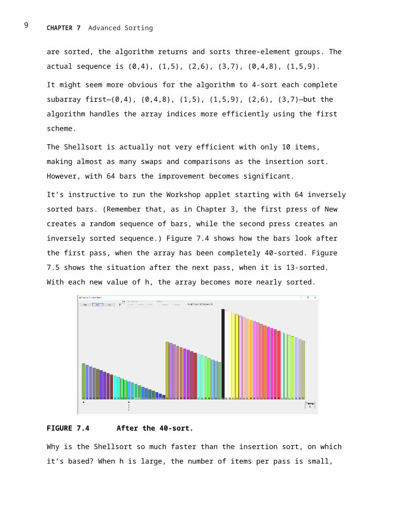
It’s instructive to run the Workshop applet starting with 64 inversely sorted bars. (Remember that, as in

Chapter 3, the first press of New creates a random sequence of bars, while the second press creates an

inversely sorted sequence.) Figure 7.4 shows how the bars look after the first pass, when the array has

been completely 40-sorted. Figure 7.5 shows the situation after the next pass, when it is 13-sorted. With

each new value of h, the array becomes more nearly sorted.


FIGURE 7.4 After the 40-sort.

Why is the Shellsort so much faster than the insertion sort, on which it’s based? When h is large, the

number of items per pass is small, and items move long distances. This is very efficient. As h grows

smaller, the number of items per pass increases, but the items are already closer to their final sorted

positions, which is more efficient for the insertion sort. It’s the combination of these trends that makes

the Shellsort so effective.

FIGURE 7.5 After the 13-sort.

Notice that later sorts (small values of h) don’t undo the work of earlier sorts (large values of h). An array

that has been 40-sorted remains 40-sorted after a 13-sort, for example. If this wasn’t so, the Shellsort

couldn’t work.


C++ Code for the Shellsort

The C++ code for the Shellsort is scarcely more complicated than for the insertion sort. Starting with the

insertion sort, you substitute h for 1 in appropriate places and add the formula to generate the interval

sequence. We’ve made shellSort() a

method in the ArraySh class, a version of the array classes from Chapter 2, “Arrays.” Listing 7.1 shows

the complete shellSort.cpp program.

LISTING 7.1 The shellSort.cpp Program

#include <iostream>#include <iomanip>#include "shellSort.h"

using namespace std;

//LISTING 7.1 The shellSort.cpp Program

// demonstrates shell sort// to run this program: C>ShellSortApp.exe//--------------------------------------------------------------

ArraySh::ArraySh() // constructor{

theArray = new long[10]; // create the array nElems = 0; // no items yet

}ArraySh::ArraySh(int max) // constructor{

theArray = new long[max];// create the array nElems = 0; // no items yet

}ArraySh::~ArraySh() //deconstructor{

delete theArray; // create the array }//-------------------------------------------------------------- void ArraySh::insert(long value) // put element into array{

theArray[nElems] = value;// insert it nElems++; // increment size

}//--------------------------------------------------------------


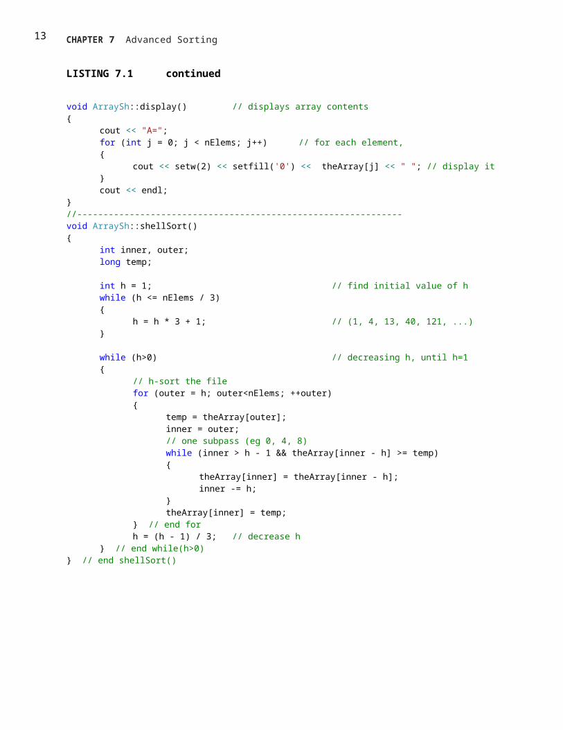
LISTING 7.1 continued

void ArraySh::display() // displays array contents{

cout << "A=";for (int j = 0; j < nElems; j++) // for each element, {

cout << setw(2) << setfill('0') << theArray[j] << " "; // display it}cout << endl;

}//-------------------------------------------------------------- void ArraySh::shellSort(){

int inner, outer;long temp;

int h = 1; // find initial value of h while (h <= nElems / 3){

h = h * 3 + 1; // (1, 4, 13, 40, 121, ...)}

while (h>0) // decreasing h, until h=1{

// h-sort the file for (outer = h; outer<nElems; ++outer){

temp = theArray[outer];inner = outer;// one subpass (eg 0, 4, 8)while (inner > h - 1 && theArray[inner - h] >= temp){

theArray[inner] = theArray[inner - h];inner -= h;

}theArray[inner] = temp;

} // end forh = (h - 1) / 3; // decrease h

} // end while(h>0)} // end shellSort()


LISTING 7.1 continued//LISTING 7.1 The shellSortApp.cpp Program

// demonstrates shell sort// to run this program: C>ShellSortApp.exe//-------------------------------------------------------------- #include <iostream>#include <ctime>#include "shellSort.h"


void main(){

int maxSize = 10; // array sizeArraySh arr = ArraySh(maxSize); // create the array

srand(static_cast<int>(time(0)));for(int j=0; j<maxSize; j++) // fill array with{ // random numbers

long n = rand() % 99 + 1; arr.insert(n);

}arr.display(); // display unsorted array arr.shellSort(); // shell sort the array arr.display(); // display sorted arrayreturn;} // end class ShellSortApp

In main() we create an object of type ArraySh, able to hold 10 items, fill it with random data, display it,

Shellsort it, and display it again. Here’s some sample output:

A=20 89 6 42 55 59 41 69 75 66

A=6 20 41 42 55 59 66 69 75 89

You can change maxSize to higher numbers, but don’t go too high; 10,000 items take a fraction of a

minute to sort.

The Shellsort algorithm, although it’s implemented in just a few lines, is not simple to follow. To see the

details of its operation, step through a 10-item sort with the Workshop applet, comparing the messages

generated by the applet with the code in the shellSort() method.

Other Interval Sequences

Picking an interval sequence is a bit of a black art. Our discussion so far used the formula h=h*3+1 to

generate the interval sequence, but other interval sequences have been used with varying degrees of


success. The only absolute requirement is that the diminishing sequence ends with 1, so the last pass is

a normal insertion sort.

In Shell’s original paper, he suggested an initial gap of N/2, which was simply divided in half for each

pass. Thus, the descending sequence for N=100 is 50, 25, 12, 6, 3, 1. This approach has the advantage

that you don’t need to calculate the sequence before the sort begins to find the initial gap; you just

divide N by 2. However, this turns out not to be the best sequence. Although it’s still better than the

insertion sort for most data, it sometimes degenerates to O(N2) running time, which is no better than

the insertion sort.

A variation of this approach is to divide each interval by 2.2 instead of 2. For n=100 this leads to 45, 20,

9, 4, 1. This is considerably better than dividing by 2, as it avoids some worst-case circumstances that

lead to O(N2) behavior. Some extra code is needed to ensure that the last value in the sequence is 1, no

matter what N is. This gives results comparable to Knuth’s sequence shown in the listing.

Another possibility for a descending sequence (from Flamig; see Appendix B) is

if(h < 5)

h = 1;

else

h = (5*h-1) / 11;

It’s generally considered important that the numbers in the interval sequence are relatively prime; that

is, they have no common divisors except 1. This constraint makes it more likely that each pass will

intermingle all the items sorted on the previous pass. The inefficiency of Shell’s original N/2 sequence is

due to its failure to adhere to this rule.

You may be able to invent a gap sequence of your own that does just as well (or possibly even better)

than those shown. Whatever it is, it should be quick to calculate so as not to slow down the algorithm.

Efficiency of the Shellsort

No one so far has been able to analyze the Shellsort’s efficiency theoretically, except in special cases.

Based on experiments, there are various estimates, which range from 0(N3/2) down to O(N7/6).


Table 7.2 shows some of these estimated O() values, compared with the slower insertion sort and the

faster quicksort. The theoretical times corresponding to various values of N are shown. Note that Nx/y

means the yth root of N raised to the x power. Thus, if N is 100, N3/2 is the square root of 1003, which is

1,000. Also, (logN)2 means the log of N, squared. This is often written log2N, but that’s easy to confuse

with log2 N, the logarithm to the base 2 of N.

TABLE 7.2 Estimates of Shellsort Running Time

O() Value Type of Sort 10 Items 100 Items 1,000 Items 10,000 Items

N2 Insertion, etc. 100 10,000 1,000,000 100,000,000

N3/2 Shellsort 32 1,000 32,000 1,000,000

N*(logN)2 Shellsort 10 400 9,000 160,000

N5/4 Shellsort 18 316 5,600 100,000

N7/6 Shellsort 14 215 3,200 46,000

N*logN Quicksort, etc. 10 200 3,000 40,000

For most data, the higher estimates, such as N3/2, are probably more realistic.

Partitioning

Partitioning is the underlying mechanism of quicksort, which we’ll explore next, but it’s also a useful

operation on its own, so we’ll cover it here in its own section.

To partition data is to divide it into two groups, so that all the items with a key value higher than a

specified amount are in one group, and all the items with a lower key value are in another.

You can easily imagine situations in which you would want to partition data. Maybe you want to divide

your personnel records into two groups: employees who live within 15 miles of the office and those who

live farther away. Or a school administrator might want to divide students into those with grade point

averages higher and lower than 3.5, so as to know who deserves to be on the Dean’s list.


The Partition Workshop Applet

Our Partition Workshop applet demonstrates the partitioning process. Figure 7.6 shows 16 bars before

partitioning, and Figure 7.7 shows them again after partitioning.

FIGURE 7.6 Sixteen bars before partitioning.

FIGURE 7.7 Sixteen bars after partitioning.


The horizontal line represents the pivot value, which is the value used to determine into which of the

two groups an item is placed. Items with a key value less than the pivot value go in the left part of the

array, and those with a greater (or equal) key go in the right part. (In the section on quicksort, we’ll see

that the pivot value can be the key value of an actual data item, called the pivot. For now, it’s just a

number.)

The arrow labeled partition points to the leftmost item in the right (higher) subarray. This value is

returned from the partitioning method, so it can be used by other methods that need to know where

the division is. For a more vivid display of the partitioning process, set the Partition Workshop applet to

100 bars and press the Run button. The leftScan and rightScan pointers will zip toward each other,

swapping bars as they go. When they meet, the partition is complete.

You can choose any value you want for the pivot value, depending on why you’re doing the partition

(such as choosing a grade point average of 3.5). For variety, the Workshop applet chooses a random

number for the pivot value (the horizontal line) each time New or Size is pressed, but the value is never

too far from the average bar height.

After being partitioned, the data is by no means sorted; it has simply been divided into two groups.

However, it’s more sorted than it was before. As we’ll see in the next section, it doesn’t take much more

trouble to sort it completely.

Notice that partitioning is not stable. That is, each group is not in the same order it was originally. In

fact, partitioning tends to reverse the order of some of the data in each group.

The partition.cpp Program

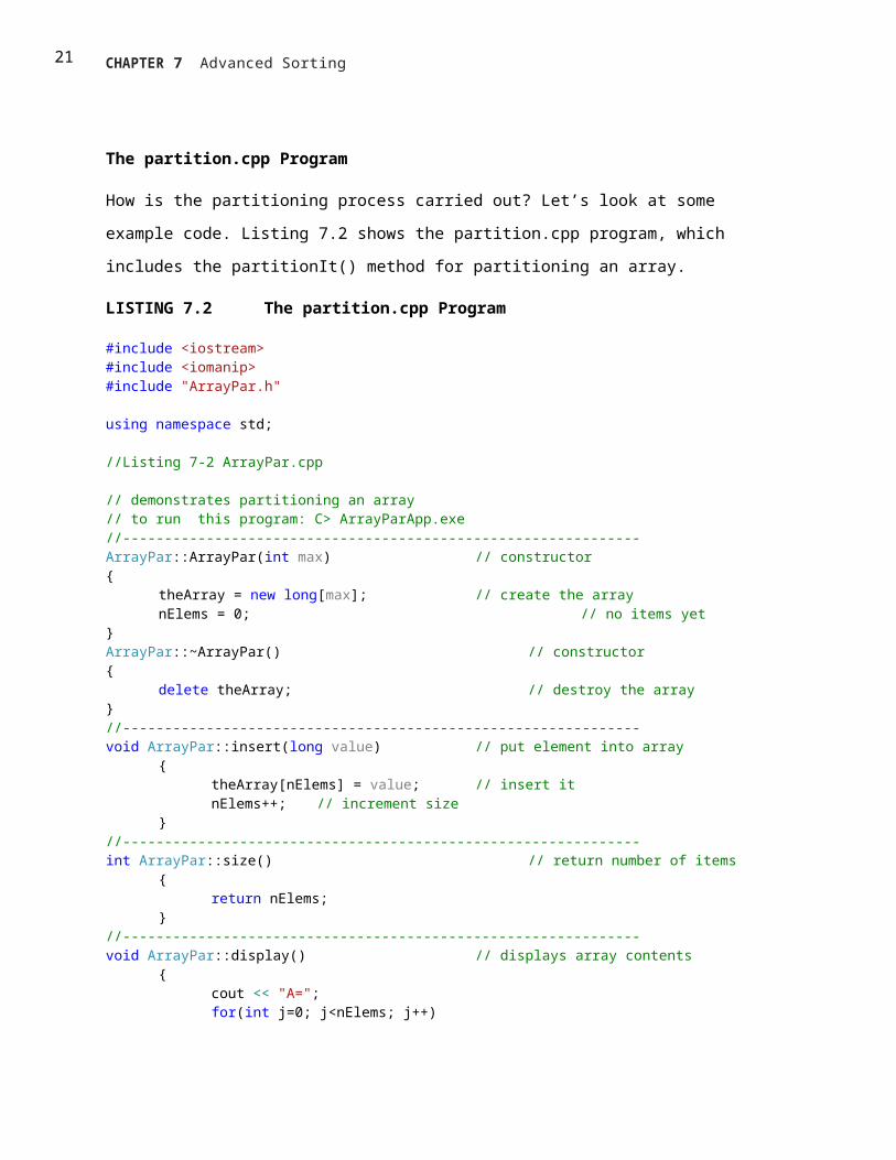
How is the partitioning process carried out? Let’s look at some example code. Listing 7.2 shows the

partition.cpp program, which includes the partitionIt() method for partitioning an array.

LISTING 7.2 The partition.cpp Program

#include <iostream>#include <iomanip>#include "ArrayPar.h"


//Listing 7-2 ArrayPar.cpp

// demonstrates partitioning an array


// to run this program: C> ArrayParApp.exe//-------------------------------------------------------------- ArrayPar::ArrayPar(int max) // constructor{

theArray = new long[max]; // create the array nElems = 0; // no items yet

}ArrayPar::~ArrayPar() // constructor{

delete theArray; // destroy the array }//-------------------------------------------------------------- void ArrayPar::insert(long value) // put element into array

{theArray[nElems] = value; // insert itnElems++; // increment size

}//-------------------------------------------------------------- int ArrayPar::size() // return number of items

{return nElems;

}//-------------------------------------------------------------- void ArrayPar::display() // displays array contents

{cout << "A=";for(int j=0; j<nElems; j++){ // for each

element,cout << setw(3) << setfill('0') << theArray[j] << " "; //

display it}cout << endl;

}//--------------------------------------------------------------


LISTING 7.2 Continued

int ArrayPar::partitionIt(int left, int right, long pivot){

int leftPtr = left - 1; // right of first elem int rightPtr = right + 1; // left of pivotwhile(true){ // find bigger

item while(leftPtr < right && theArray[++leftPtr] < pivot); //nop

// find smaller item

while(rightPtr > left && theArray[--rightPtr] > pivot); // (nop)

if(leftPtr >= rightPtr) // if pointers cross, break; // partition done

else // not crossed, so swap(leftPtr, rightPtr);// swap elements

} // end while(true)return leftPtr; // return partition

} // end partitionIt()//--------------------------------------------------------------

void ArrayPar::swap(int dex1, int dex2) // swap two elements{

long temp;temp = theArray[dex1]; // A into temp theArray[dex1] = theArray[dex2]; // B into A theArray[dex2] = temp; // temp into B

} // end swap()//--------------------------------------------------------------////////////////////////////////////////////////////////////////

#include <iostream>#include <ctime>#include "ArrayPar.h"


//Listing 7-2 ArrayParApp.cpp

// demonstrates partitioning an array// to run this program: C> ArrayParApp.exe//--------------------------------------------------------------

void main(){

int maxSize = 16; // array sizeArrayPar *arr = new ArrayPar(maxSize); // create the array

srand(static_cast<int>(time(0)));for(int j=0; j<maxSize; j++) // fill array with{ // random numbers

long n = rand() %199 + 1; arr->insert(n);

}


arr->display(); // display unsorted arraylong pivot = 99; // pivot valuecout << "Pivot is " << pivot;


int size = arr->size();

// partition array int partDex = arr->partitionIt(0, size-1, pivot);cout << ", Partition is at index " << partDex << endl;

// display partitioned arrayarr->display();

} // end main()

The main() routine creates an ArrayPar object that holds 16 items of type long. The pivot value is fixed at

99. The routine inserts 16 random values into ArrayPar, displays them, partitions them by calling the

partitionIt() method, and displays them again. Here’s some sample output:

A=149 192 47 152 159 195 61 66 17 167 118 64 27 80 30 105Pivot is 99, partition is at index 8A=30 80 47 27 64 17 61 66 195 167 118 159 152 192 149 105

You can see that the partition is successful: The first eight numbers are all smaller than the pivot value of

99; the last eight are all larger.

Notice that the partitioning process doesn’t necessarily divide the array in half as it does in this example;

that depends on the pivot value and key values of the data. There may be many more items in one

group than in the other.

The Partition Algorithm

The partitioning algorithm works by starting with two pointers, one at each end of the array. (We use

the term pointers to mean indices that point to array elements, not C++ pointers.) The pointer on the

left, leftPtr, moves toward the right, and the one on the right, rightPtr, moves toward the left. Notice

that leftPtr and rightPtr in the partition.cpp program correspond to leftScan and rightScan in the

Partition Workshop applet.

Actually, leftPtr is initialized to one position to the left of the first cell, and rightPtr to one position to the

right of the last cell, because they will be incremented and decremented, respectively, before they’re

used.


Stopping and Swapping

When leftPtr encounters a data item smaller than the pivot value, it keeps going because that item is

already on the correct side of the array. However, when it encounters an item larger than the pivot

value, it stops. Similarly, when rightPtr encounters an item larger than the pivot, it keeps going, but

when it finds a smaller item, it also stops. Two inner while loops, the first for leftPtr and the second for

rightPtr, control the scanning process. A pointer stops because its while loop exits. Here’s a simplified

version of the code that scans for out-of-place items:

while( theArray[++leftPtr] < pivot ) // find bigger item; // (nop)

while( theArray[--rightPtr] > pivot ) // find smaller item; // (nop)

swap(leftPtr, rightPtr); // swap elements

The first while loop exits when an item larger than pivot is found; the second loop exits when an item

smaller than pivot is found. When both these loops exit, both leftPtr and rightPtr point to items that are

in the wrong sides of the array, so these items are swapped.

After the swap, the two pointers continue on, again stopping at items that are in the wrong side of the

array and swapping them. All this activity is nested in an outer while loop, as can be seen in the

partitionIt() method in Listing 7.2. When the two pointers eventually meet, the partitioning process is

complete and this outer while loop exits.

You can watch the pointers in action when you run the Partition Workshop applet with 100 bars. These

pointers, represented by blue arrows, start at opposite ends of the array and move toward each other,

stopping and swapping as they go. The bars between them are unpartitioned; those they’ve already

passed over are partitioned. When they meet, the entire array is partitioned.

Handling Unusual Data

If we were sure that there was a data item at the right end of the array that was smaller than the pivot

value, and an item at the left end that was larger, the simplified while loops previously shown would

work fine. Unfortunately, the algorithm may be called upon to partition data that isn’t so well organized.

If all the data is smaller than the pivot value, for example, the leftPtr variable will go all the way across


the array, looking in vain for a larger item, and fall off the right end, creating an array index out of

bounds exception. A similar fate will befall rightPtr if all the data is larger than the pivot value.

To avoid these problems, extra tests must be placed in the while loops to check for the ends of the

array: leftPtr<right in the first loop and rightPtr>left in the second. You can see these tests in context in

Listing 7.2.

In the section on quicksort, we’ll see that a clever pivot-selection process can eliminate these end-of-

array tests. Eliminating code from inner loops is always a good idea if you want to make a program run

faster.

Delicate Code

The code in the while loops is rather delicate. For example, you might be tempted to remove the

increment operators from the inner while loops and use them to replace the nop statements. (Nop

refers to a statement consisting only of a semicolon, and means no operation). For example, you might

try to change this:

while(leftPtr < right && theArray[++leftPtr] < pivot); // (nop)

to this:while(leftPtr < right && theArray[leftPtr] < pivot)++leftPtr;

and similarly for the other inner while loop. These changes would make it possible for the initial values

of the pointers to be left and right, which is somewhat clearer than left-1 and right+1.

However, these changes result in the pointers being incremented only when the condition is satisfied.

The pointers must move in any case, so two extra statements within the outer while loop would be

required to bump the pointers. The nop version is the most efficient solution.

Equal Keys

Here’s another subtle change you might be tempted to make in the partitionIt() code. If you run the

partitionIt() method on items that are all equal to the pivot value, you will find that every comparison

leads to a swap. Swapping items with equal keys seems like a waste of time. The < and > operators that

compare pivot with the array elements in the while loops cause the extra swapping. However, suppose


you try to fix this by replacing them with <= and >= operators. This indeed prevents the swapping of

equal elements, but it also causes leftPtr and rightPtr to end up at the ends of the array when the

algorithm has finished. As we’ll see in the section on quicksort, it’s good for the pointers to end up in the

middle of the array, and very bad for them to end up at the ends. So if partitionIt() is going to be used

for quicksort, the < and > operators are the right way to go, even if they cause some unnecessary

swapping.

Efficiency of the Partition Algorithm

The partition algorithm runs in O(N) time. It’s easy to see why this is so when running the Partition

Workshop applet: The two pointers start at opposite ends of the array and move toward each other at a

more or less constant rate, stopping and swapping as they go. When they meet, the partition is

complete. If there were twice as many items to partition, the pointers would move at the same rate, but

they would have twice as many items to compare and swap, so the process would take twice as long.

Thus, the running time is proportional to N.

More specifically, for each partition there will be N+1 or N+2 comparisons. Every item will be

encountered and used in a comparison by one or the other of the pointers, leading to N comparisons,

but the pointers overshoot each other before they find out they’ve “crossed” or gone beyond each

other, so there are one or two extra comparisons before the partition is complete. The number of

comparisons is independent of how the data is arranged (except for the uncertainty between one or two

extra comparisons at the end of the scan).

The number of swaps, however, does depend on how the data is arranged. If it’s inversely ordered, and

the pivot value divides the items in half, then every pair of values must be swapped, which is N/2 swaps.

(Remember in the Partition Workshop applet that the pivot value is selected randomly, so that the

number of swaps for inversely sorted bars won’t always be exactly N/2.)

For random data, there will be fewer than N/2 swaps in a partition, even if the pivot value is such that

half the bars are shorter and half are taller. This is because some bars will already be in the right place

(short bars on the left, tall bars on the right). If the pivot value is higher (or lower) than most of the bars,

there will be even fewer swaps because only those few bars that are higher (or lower) than the pivot will

need to be swapped. On average, for random data, about half the maximum number of swaps take

place.


Although there are fewer swaps than comparisons, they are both proportional to N. Thus, the

partitioning process runs in O(N) time. Running the Workshop applet, you can see that for 12 random

bars there are about 3 swaps and 14 comparisons, and for 100 random bars there are about 25 swaps

and 102 comparisons.

Quicksort

Quicksort is undoubtedly the most popular sorting algorithm, and for good reason: In the majority of

situations, it’s the fastest, operating in O(N*logN) time. (This is only true for internal or in-memory

sorting; for sorting data in disk files, other algorithms may be better.) Quicksort was discovered by C.A.R.

Hoare in 1962.

To understand quicksort, you should be familiar with the partitioning algorithm described in the

preceding section. Basically, the quicksort algorithm operates by partitioning an array into two subarrays

and then calling itself recursively to quicksort each of these subarrays. However, there are some

embellishments we can make to this basic scheme. They have to do with the selection of the pivot and

the sorting of small partitions. We’ll examine these refinements after we’ve looked at a simple version

of the main algorithm.

It’s difficult to understand what quicksort is doing before you understand how it does it, so we’ll reverse

our usual presentation and show the C++ code for quicksort before presenting the QuickSort1 Workshop

applet.

The Quicksort Algorithm

The code for a basic recursive quicksort method is fairly simple. Here’s an example:

void recQuickSort(int left, int right){

if (right - left <= 0) // if size <= 1, return; // already sorted

else // size is 2 or larger{

long pivot = theArray[right]; // rightmost item// partition range

int partition = partitionIt(left, right);recQuickSort(left, partition - 1); // sort left side recQuickSort(partition + 1, right); // sort right side

}} // end recQuickSort()


}

As you can see, there are three basic steps:

1. Partition the array or subarray into left (smaller keys) and right (larger keys) groups.

2. Call ourselves to sort the left group.

3. Call ourselves again to sort the right group.

After a partition, all the items in the left subarray are smaller than all those on the right. If we then sort

the left subarray and sort the right subarray, the entire array will be sorted. How do we sort these

subarrays? By calling our self recursively.

The arguments to the recQuickSort() method determine the left and right ends of the array (or subarray)

it’s supposed to sort. The method first checks if this array consists of only one element. If so, the array is

by definition already sorted, and the method returns immediately. This is the base case in the recursion

process.

If the array has two or more cells, the algorithm calls the partitionIt() method, described in the

preceding section, to partition it. This method returns the index number of the partition: the left

element in the right (larger keys) subarray. The partition marks the boundary between the subarrays.

This situation is shown in Figure 7.8.


FIGURE 7.8 Recursive calls sort subarrays.

After the array is partitioned, recQuickSort() calls itself recursively, once for the left part of its array,

from left to partition-1, and once for the right, from partition+1 to right. Note that the data item at the

index partition is not included in either of the recursive calls. Why not? Doesn’t it need to be sorted?

The explanation lies in how the pivot value is chosen.

Choosing a Pivot Value

What pivot value should the partitionIt() method use? Here are some relevant ideas:

• The pivot value should be the key value of an actual data item; this item is called the pivot.

• You can pick a data item to be the pivot more or less at random. For simplicity, let’s say we always pick

the item on the right end of the subarray being partitioned.

• After the partition, if the pivot is inserted at the boundary between the left and right subarrays, it will

be in its final sorted position.


This last point may sound unlikely, but remember that, because the pivot’s key value is used to partition

the array, following the partition the left subarray holds items smaller than the pivot, and the right

subarray holds items larger. The pivot starts out on the right, but if it could somehow be placed between

these two subarrays, it would be in the correct place—that is, in its final sorted position. Figure 7.9

shows how this looks with a pivot whose key value is 36.

FIGURE 7.9 The pivot and the subarrays.

This figure is somewhat fanciful because you can’t actually take an array apart as we’ve shown. So how

do we move the pivot to its proper place?

We could shift all the items in the right subarray to the right one cell to make room for the pivot.

However, this is inefficient and unnecessary. Remember that all the items in the right subarray, although

they are larger than the pivot, are not yet sorted, so they can be moved around, within the right

subarray, without affecting anything. Therefore, to simplify inserting the pivot in its proper place, we can

simply swap the pivot (36) and the left item in the right subarray, which is 63. This swap places the pivot

in its proper position between the left and right groups. The 63 is switched to the right end, but because

it remains in the right (larger) group, the partitioning is undisturbed. This situation is shown in Figure

7.10.


FIGURE 7.10 Swapping the pivot.

When it’s swapped into the partition’s location, the pivot is in its final resting place. All subsequent

activity will take place on one side of it or on the other, but the pivot itself won’t be moved (or indeed

even accessed) again.

To incorporate the pivot selection process into our recQuickSort() method, let’s make it an overt

statement, and send the pivot value to partitionIt() as an argument. Here’s how that looks:

void recQuickSort(int left, int right){




int partition = partitionIt(left, right, pivot);recQuickSort(left, partition - 1); // sort left side recQuickSort(partition + 1, right); // sort right side

}} // end recQuickSort()

}When we use this scheme of choosing the rightmost item in the array as the pivot, we’ll need to modify

the partitionIt() method to exclude this rightmost item from the partitioning process; after all, we


already know where it should go after the partitioning process is complete: at the partition, between the

two groups. Also, after the partitioning process is completed, we need to swap the pivot from the right

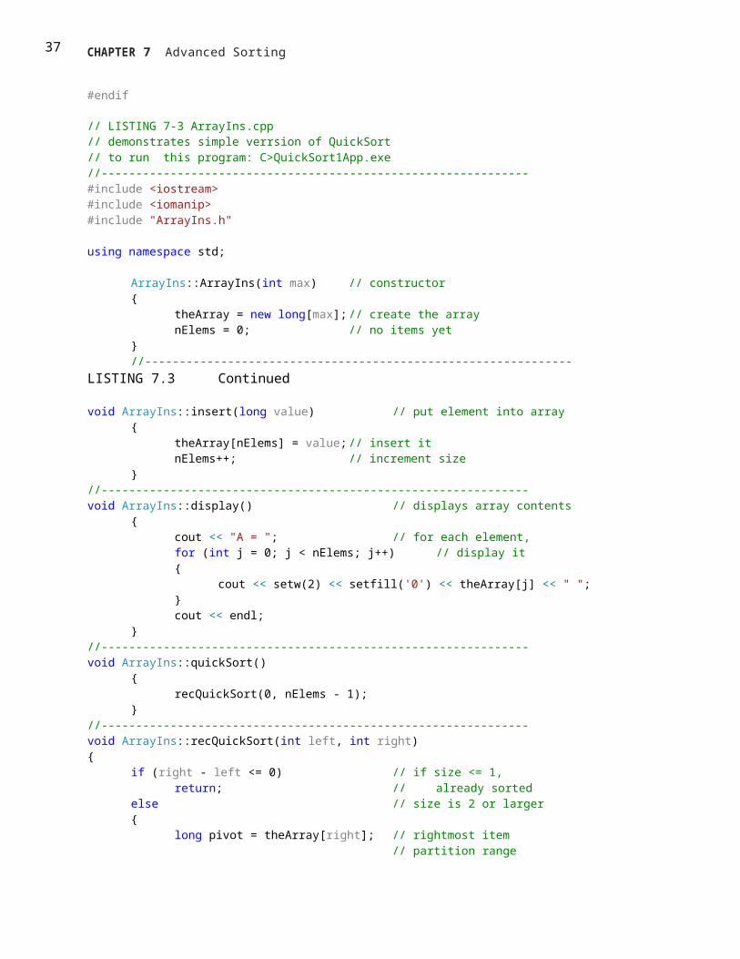
end into the partition’s location. Listing 7.3 shows the quickSort1.cpp program, which incorporates these

features.

LISTING 7.3 The quickSort1.cpp Program

// LISTING 7-3 ArrayIns.h// demonstrates simple verrsion of QuickSort// to run this program: C>QuickSort1App.exe//-------------------------------------------------------------- #ifndef _ArrayIns#define _ArrayIns

class ArrayIns{private:

long *theArray; // ref to array theArray int nElems; // number of data items

//-------------------------------------------------------------- public:

ArrayIns(int); // constructor//--------------------------------------------------------------

void insert(long); // put element into array//--------------------------------------------------------------

void display(); // displays array contents//--------------------------------------------------------------

void quickSort();//--------------------------------------------------------------

void recQuickSort(int, int);//--------------------------------------------------------------

int partitionIt(int, int, long);//--------------------------------------------------------------

void swap(int, int); // swap two elements//--------------------------------------------------------------}; // end class ArrayIns#endif

// LISTING 7-3 ArrayIns.cpp// demonstrates simple verrsion of QuickSort// to run this program: C>QuickSort1App.exe//-------------------------------------------------------------- #include <iostream>#include <iomanip>#include "ArrayIns.h"


ArrayIns::ArrayIns(int max) // constructor{

theArray = new long[max];// create the array nElems = 0; // no items yet

}//--------------------------------------------------------------



void ArrayIns::insert(long value) // put element into array{

theArray[nElems] = value;// insert it nElems++; // increment size

}//-------------------------------------------------------------- void ArrayIns::display() // displays array contents

{cout << "A = "; // for each element, for (int j = 0; j < nElems; j++) // display it{

cout << setw(2) << setfill('0') << theArray[j] << " ";}cout << endl;

}//-------------------------------------------------------------- void ArrayIns::quickSort()

{recQuickSort(0, nElems - 1);

}//-------------------------------------------------------------- void ArrayIns::recQuickSort(int left, int right){




int partition = partitionIt(left, right, pivot);recQuickSort(left, partition - 1); // sort left side recQuickSort(partition + 1, right); // sort right side

}} // end recQuickSort()//-------------------------------------------------------------- int ArrayIns::partitionIt(int left, int right, long pivot)

{int leftPtr = left - 1; // left (after ++) int rightPtr = right; // right-1 (after --) while (true){ // find bigger item

while (theArray[++leftPtr] < pivot) ; // (nop)// find smaller item while (rightPtr > 0 && theArray[--rightPtr] > pivot); // (nop)

if (leftPtr >= rightPtr) // if pointers cross, break; // partition done

else // not crossed, so swap(leftPtr, rightPtr); // swap elements

} // end while(true)swap(leftPtr, right); // restore pivotreturn leftPtr; // return pivot location} // end partitionIt()

//--------------------------------------------------------------



void ArrayIns::swap(int dex1, int dex2) // swap two elements{

long temp = theArray[dex1]; // A into temp theArray[dex1] = theArray[dex2]; // B into A theArray[dex2] = temp; // temp into B

} // end swap( //--------------------------------------------------------------

#include <iostream>#include <iomanip>#include <ctime>#include "ArrayIns.h"


void main(){

int maxSize = 16; // array sizeArrayIns *arr = new ArrayIns(maxSize); // create array

srand(static_cast<int>(time(0)));for (int j = 0; j<maxSize; j++){

long n = rand() % 99 + 1; // fill array witharr->insert(n); // random numbers

}arr->display(); // display items arr->quickSort(); // quicksort them arr->display(); // display them again

} // end main()

The main() routine creates an object of type ArrayIns, inserts 16 random data items of type long in it,

displays it, sorts it with the quickSort() method, and displays the results. Here’s some typical output:

A=69 0 70 6 38 38 24 56 44 26 73 77 30 45 97 65

A=0 6 24 26 30 38 38 44 45 56 65 69 70 73 77 97

An interesting aspect of the code in the partitionIt() method is that we’ve been able to remove the test

for the end of the array in the first inner while loop. This test, seen in the earlier partitionIt() method in

the partition.cpp program in Listing 7.2, was

leftPtr < right

It prevented leftPtr running off the right end of the array if no item there was larger than pivot. Why can

we eliminate the test? Because we selected the rightmost item as the pivot, so leftPtr will always stop


there. However, the test is still necessary for rightPtr in the second while loop. (Later we’ll see how this

test can be eliminated as well.)

Choosing the rightmost item as the pivot is thus not an entirely arbitrary choice; it speeds up the code

by removing an unnecessary test. Picking the pivot from some other location would not provide this

advantage.

The QuickSort1 Workshop Applet

At this point you know enough about the quicksort algorithm to understand the nuances of the

QuickSort1 Workshop applet.

The Big Picture

For the big picture, use the Size button to set the applet to sort 64 random bars, and press the Run

button. Following the sorting process, the display will look something like Figure 7.11.

FIGURE 7.11 The QuickSort1 Workshop applet with 64 bars.

Watch how the algorithm partitions the array into two parts, then sorts each of these parts by

partitioning it into two parts, and so on, creating smaller and smaller subarrays.

When the sorting process is complete, each dotted line provides a visual record of one of the sorted

subarrays. The horizontal range of the line shows which bars were part of the subarray, and its vertical

position is the pivot value (the height of the pivot). The total length of all these lines on the display is a


measure of how much work the algorithm has done to sort the array; we’ll return to this topic later.

Each dotted line (except the shortest ones) should have a line below it (probably separated by other,

shorter lines) and a line above it that together add up to the same length as the original line (less one

bar). These are the two partitions into which each subarray is divided.

The Details

For a more detailed examination of quicksort’s operation, switch to the 12-bar display in the QuickSort1

Workshop applet and step through the sorting process. You’ll see how the pivot value corresponds to

the height of the pivot on the right

side of the array and how the algorithm partitions the array, swaps the pivot into the space between the

two sorted groups, sorts the shorter group (using many recursive calls), and then sorts the larger group.

Figure 7.12 shows all the steps involved in sorting 12 bars. The horizontal brackets under the arrays

show which subarray is being partitioned at each step, and the circled numbers show the order in which

these partitions are created. A pivot being swapped into place is shown with a dotted arrow. The final

position of the pivot is shown as a dotted cell to emphasize that this cell contains a sorted item that will

not be changed thereafter. Horizontal brackets under single cells (steps 5, 6, 7, 11, and

12) are base case calls to recQuickSort(); they return immediately.

Sometimes, as in steps 4 and 10, the pivot ends up in its original position on the right side of the array

being sorted. In this situation, there is only one subarray remaining to be sorted: the one to the left of

the pivot. There is no second subarray to its right.

The different steps in Figure 7.12 occur at different levels of recursion, as shown in Table 7.3. The initial

call from main() to recQuickSort() is the first level, recQuickSort() calling two new instances of itself is

the second level, these two instances calling four more instances is the third level, and so on.

TABLE 7.3 Recursion Levels for Figure 7.12

Step Recursion Level

1 1

2, 8 2

3, 7, 9, 12 3

4, 10 4


5, 6, 11 5


FIGURE 7.12 The quicksort process.


The order in which the partitions are created, corresponding to the step numbers, does not correspond

with depth. It’s not the case that all the first-level partitions are done first, then all the second level

ones, and so on. Instead, the left group at every level is handled before any of the right groups.

In theory there should be 8 steps in the fourth level and 16 in the fifth level, but in this small array we

run out of items before these steps are necessary.

The number of levels in the table shows that with 12 data items, the machine stack needs enough space

for 5 sets of arguments and return values; one for each recursion level. This is, as we’ll see later,

somewhat greater than the logarithm to the base 2 of the number of items: log N. The size of the

machine stack is determined by your particular system. Sorting very large numbers of data items using

recursive procedures may cause this stack to overflow, leading to memory errors.

Things to Notice

Here are some details you may notice as you run the QuickSort1 Workshop applet.

You might think that a powerful algorithm like quicksort would not be able to handle subarrays as small

as two or three items. However, this version of the quicksort algorithm is quite capable of sorting such

small subarrays; leftScan and rightScan just don’t go very far before they meet. For this reason we don’t

need to use a different sorting scheme for small subarrays. (Although, as we’ll see later, handling small

subarrays differently may have advantages.)

At the end of each scan, the leftScan variable ends up pointing to the partition— that is, the left element

of the right subarray. The pivot is then swapped with the partition to put the pivot in its proper place, as

we’ve seen. As we noted, in steps 3 and 9 of Figure 7.12, leftScan ends up pointing to the pivot itself, so

the swap has no effect. This may seem like a wasted swap; you might decide that leftScan should stop

one bar sooner. However, it’s important that leftScan scan all the way to the pivot; otherwise, a swap

would unsort the pivot and the partition.

Be aware that leftScan and rightScan start at left-1 and right. This may look peculiar on the display,

especially if left is 0; then leftScan will start at –1. Similarly,

rightScan initially points to the pivot, which is not included in the partitioning process. These pointers

start outside the subarray being partitioned because they will be incremented and decremented,

respectively, before they’re used the first time.

The applet shows ranges as numbers in parentheses; for example, (2-5) means the subarray from index


2 to index 5. The range given in some of the messages may be negative: from a higher number to a

lower one, such as Array partitioned; left (7-6), right (8-8). The (8-8) range means a single cell (8), but

what does (7-6) mean? This range isn’t real; it simply reflects the values that left and right, the

arguments to recQuickSort(), have when this method is called. Here’s the code in question:

int partition = partitionIt(left, right, pivot); recQuickSort(left, partition-1); // sort left side

recQuickSort(partition+1, right); // sort right side

If partitionIt() is called with left = 7 and right = 8, for example, and happens to return 7 as the partition,

then the range supplied in the first call to recQuickSort() will be (7-6) and the range to the second will be

(8-8). This is normal. The base case in recQuickSort() is activated by array sizes less than 1 as well as by 1,

so it will return immediately for negative ranges. Negative ranges are not shown in Figure

7.12, although they do cause (brief) calls to recQuickSort().

Degenerates to O(N2) Performance

If you use the QuickSort1 Workshop applet to sort 100 inversely sorted bars, you’ll see that the

algorithm runs much more slowly and that many more dotted horizontal lines are generated, indicating

more and larger subarrays are being partitioned. What’s happening here?

The problem is in the selection of the pivot. Ideally, the pivot should be the median of the items being

sorted. That is, half the items should be larger than the pivot, and half smaller. This would result in the

array being partitioned into two subarrays of equal size. Having two equal subarrays is the optimum

situation for the quicksort algorithm. If it has to sort one large and one small array, it’s less efficient

because the larger subarray has to be subdivided more times.

The worst situation results when a subarray with N elements is divided into one subarray with 1 element

and the other with N-1 elements. (This division into 1 cell and N-1 cells can also be seen in steps 3 and 9

in Figure 7.12.) If this 1 and N-1 division happens with every partition, then every element requires a

separate partition step. This is in fact what takes place with inversely sorted data: In all the subarrays,

the pivot is the smallest item, so every partition results in N-1 elements in one subarray and only the


pivot in the other.

To see this unfortunate process in action, step through the QuickSort1 Workshop applet with 12

inversely sorted bars. Notice how many more steps are necessary than with random data. In this

situation the advantage gained by the partitioning process is lost and the performance of the algorithm

degenerates to O(N2).

Besides being slow, there’s another potential problem when quicksort operates in O(N2) time. When the

number of partitions increases, the number of recursive function calls also increases. Every function

call takes up room on the machine stack. If there are too many calls, the machine stack may overflow

and paralyze the system.

To summarize: In the QuickSort1 applet, we select the rightmost element as the pivot. If the data is truly

random, this isn’t too bad a choice because usually the

pivot won’t be too close to either end of the array. However, when the data is sorted or inversely

sorted, choosing the pivot from one end or the other is a bad idea. Can we improve on our approach to

selecting the pivot?

Median-of-Three Partitioning

Many schemes have been devised for picking a better pivot. The method should be simple but have a

good chance of avoiding the largest or smallest value. Picking an element at random is simple but—as

we’ve seen—doesn’t always result in a good selection. However, we could examine all the elements and

actually calculate which one was the median. This would be the ideal pivot choice, but the process isn’t

prac- tical, as it would take more time than the sort itself.

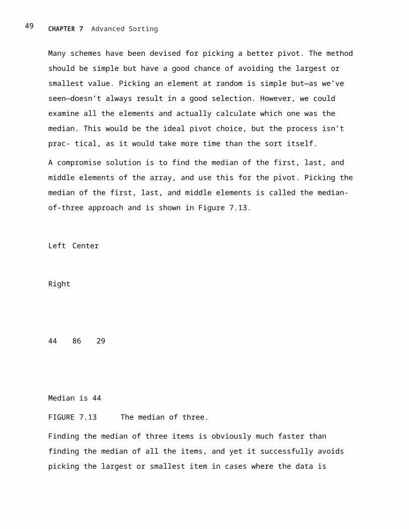
A compromise solution is to find the median of the first, last, and middle elements of the array, and use

this for the pivot. Picking the median of the first, last, and middle elements is called the median-of-three

approach and is shown in Figure 7.13.

Left Center


Right

44 86 29

Median is 44

FIGURE 7.13 The median of three.

Finding the median of three items is obviously much faster than finding the median of all the items, and

yet it successfully avoids picking the largest or smallest item in cases where the data is already sorted or

inversely sorted. There are probably some pathological arrangements of data where the median-of-

three scheme works poorly, but normally it’s a fast and effective technique for finding the pivot.

Besides picking the pivot more effectively, the median-of-three approach has an additional benefit: We

can dispense with the rightPtr>left test in the second inside while loop, leading to a small increase in the

algorithm’s speed. How is this possible?

The test can be eliminated because we can use the median-of-three approach to not only select the

pivot, but also to sort the three elements used in the selection process. Figure 7.14 shows this

operation.

When these three elements are sorted, and the median item is selected as the pivot, we are guaranteed

that the element at the left end of the subarray is less than (or equal to) the pivot, and the element at

the right end is greater than (or equal to) the

pivot. This means that the leftPtr and rightPtr indices can’t step beyond the right or left ends of the

array, respectively, even if we remove the leftPtr>right and rightPtr<left tests. (The pointer will stop,


thinking it needs to swap the item, only to find that it has crossed the other pointer and the partition is

complete.) The values at left and right act as sentinels to keep leftPtr and rightPtr confined to valid array

values.

Left Center Right

44 86 29

Before sorting

Left Center Right

29 44 86

After sorting

Becomes pivot

FIGURE 7.14 Sorting the left, center, and right elements.

Another small benefit to median-of-three partitioning is that after the left, center, and right elements

are sorted, the partition process doesn’t need to examine these elements again. The partition can begin

at left+1 and right-1 because left and right have in effect already been partitioned. We know that left is

in the correct partition because it’s on the left and it’s less than the pivot, and right is in the correct

place because it’s on the right and it’s greater than the pivot.

Thus, median-of-three partitioning not only avoids O(N2) performance for already- sorted data, it also

allows us to speed up the inner loops of the partitioning algorithm and reduce slightly the number of

items that must be partitioned.

The quickSort2.cpp Program

Listing 7.4 shows the quickSort2.cpp program, which incorporates median-of-three partitioning. We use

a separate method, medianOf3(), to sort the left, center, and right elements of a subarray. This method

returns the value of the pivot, which is then


sent to the partitionIt() method.


// quickSort2.cpp

// demonstrates quick sort with median-of-three partitioning

// to run this program: C>C++ QuickSort2App

////////////////////////////////////////////////////////////////

class ArrayIns

{

private long[] theArray; // ref to array theArray private int nElems; // number of data items

//-------------------------------------------------------------- public ArrayIns(int max) // constructor

{


}

//-------------------------------------------------------------- public void insert(long value) // put element into

array

{

theArray[nElems] = value; // insert it nElems++; // increment size

}

//-------------------------------------------------------------- public void display() // displays array contents

{ System.out.print(“A=”);

for(int j=0; j<nElems; j++) // for each element, System.out.print(theArray[j] + “ “); // display it

System.out.println(“”);


}

//-------------------------------------------------------------- public void quickSort()

{

recQuickSort(0, nElems-1);

}

//-------------------------------------------------------------- public void recQuickSort(int left, int right)

{

int size = right-left+1;

if(size <= 3) // manual sort if small manualSort(left, right);

else // quicksort if large

{

long median = medianOf3(left, right);

int partition = partitionIt(left, right, median); recQuickSort(left, partition-1); recQuickSort(partition+1,

right);

}

} // end recQuickSort()

//-------------------------------------------------------------- public long medianOf3(int left, int right)

{

int center = (left+right)/2;

// order left & center if( theArray[left] > theArray[center] )

swap(left, center);

// order left & right if( theArray[left] > theArray[right] )

swap(left, right);

// order center & right if( theArray[center] > theArray[right] )


swap(center, right);

swap(center, right-1); // put pivot on right return theArray[right-1]; // return median value

} // end medianOf3()

//-------------------------------------------------------------- public void swap(int dex1, int dex2) // swap two

elements

{

long temp = theArray[dex1]; // A into temp theArray[dex1] = theArray[dex2]; // B into A

theArray[dex2] = temp; // temp into B

} // end swap(

//-------------------------------------------------------------- public int partitionIt(int left, int right, long pivot)

{

int leftPtr = left; // right of first elem int rightPtr = right - 1; // left of pivot

while(true)

{

while( theArray[++leftPtr] < pivot ) // find bigger

; // (nop)

while( theArray[--rightPtr] > pivot ) // find smaller


; // (nop)



} // end while(true)


swap(leftPtr, right-1); // restore pivot

return leftPtr; // return pivot location

} // end partitionIt()

//-------------------------------------------------------------- public void manualSort(int left, int right)

{


if(size <= 1)

return; // no sort necessary if(size == 2)

{ // 2-sort left and right if( theArray[left] > theArray[right] )

swap(left, right);

return;

}

else // size is 3

{ // 3-sort left, center, & right if( theArray[left] > theArray[right-1] )

swap(left, right-1); // left, center if( theArray[left] > theArray[right] )

swap(left, right); // left, right if( theArray[right-1] > theArray[right] )

swap(right-1, right); // center, right

}

} // end manualSort()

//--------------------------------------------------------------

} // end class ArrayIns

////////////////////////////////////////////////////////////////

class QuickSort2App

{

public static void main(String[] args)


{

int maxSize = 16; // array size

ArrayIns arr; // reference to array arr = new ArrayIns(maxSize); // create the array

for(int j=0; j<maxSize; j++) // fill array with

{ // random numbers long n = (int)(C++.lang.Math.random()*99); arr.insert(n);

}

arr.display(); // display items arr.quickSort(); // quicksort them arr.display(); // display them again

} // end main()

} // end class QuickSort2App

This program uses another new method, manualSort(), to sort subarrays of three or fewer elements. It

returns immediately if the subarray is one cell (or less), swaps the cells if necessary if the range is 2, and

sorts three cells if the range is 3. The recQuickSort() routine can’t be used to sort ranges of 2 or 3

because median partitioning requires at least four cells.

The main() routine and the output of quickSort2.cpp are similar to those of

quickSort1.cpp.

The QuickSort2 Workshop Applet

The Quicksort2 Workshop applet demonstrates the quicksort algorithm using median-of-three

partitioning. This applet is similar to the QuickSort1 Workshop applet, but starts off sorting the first,

center, and left elements of each subarray and selecting the median of these as the pivot value. At least,

it does this if the array size is greater than 3. If the subarray is two or three units, the applet simply sorts

it “by hand” without partitioning or recursive calls.

Notice the dramatic improvement in performance when the applet is used to sort

100 inversely ordered bars. No longer is every subarray partitioned into 1 cell and

N-1 cells; instead, the subarrays are partitioned roughly in half.


Other than this improvement for ordered data, the QuickSort2 Workshop applet produces results similar

to QuickSort1. It is no faster when sorting random data; it’s advantages become evident only when

sorting ordered data.

Handling Small Partitions

If you use the median-of-three partitioning method, it follows that the quicksort algorithm won’t work

for partitions of three or fewer items. The number 3 in this case is called a cutoff point. In the examples

above we sorted subarrays of two or three items by hand. Is this the best way?

Using an Insertion Sort for Small Partitions

Another option for dealing with small partitions is to use the insertion sort. When you do this, you aren’t

restricted to a cutoff of 3. You can set the cutoff to 10, 20, or any other number. It’s interesting to

experiment with different values of the cutoff to see where the best performance lies. Knuth (see

Appendix B) recommends a cutoff of

9. However, the optimum number depends on your computer, operating system, compiler (or

interpreter), and so on.

The quickSort3.cpp program, shown in Listing 7.5, uses an insertion sort to handle subarrays of fewer

than 10 cells.


// quickSort3.cpp

// demonstrates quick sort; uses insertion sort for cleanup

// to run this program: C>C++ QuickSort3App

////////////////////////////////////////////////////////////////

class ArrayIns

{

private long[] theArray; // ref to array theArray private int nElems; // number of data items


//-------------------------------------------------------------- public ArrayIns(int max) // constructor

{


}

//-------------------------------------------------------------- public void insert(long value) // put element into

array

{

theArray[nElems] = value; // insert it nElems++; // increment size

}

//-------------------------------------------------------------- public void display() // displays array contents

{ System.out.print(“A=”);

for(int j=0; j<nElems; j++) // for each element, System.out.print(theArray[j] + “ “); // display it

System.out.println(“”);

}

//-------------------------------------------------------------- public void quickSort()

{

recQuickSort(0, nElems-1);

// insertionSort(0, nElems-1); // the other option

}

//-------------------------------------------------------------- public void recQuickSort(int left, int right)

{


if(size < 10) // insertion sort if small insertionSort(left, right);

else // quicksort if large


{

long median = medianOf3(left, right);

int partition = partitionIt(left, right, median); recQuickSort(left, partition-1); recQuickSort(partition+1,

right);

}

} // end recQuickSort()

//-------------------------------------------------------------- public long medianOf3(int left, int right)

{

int center = (left+right)/2;

// order left & center if( theArray[left] > theArray[center] )

swap(left, center);

// order left & right if( theArray[left] > theArray[right] )

swap(left, right);

// order center & right if( theArray[center] > theArray[right] )

swap(center, right);

swap(center, right-1); // put pivot on right return theArray[right-1]; // return median value

} // end medianOf3()

//-------------------------------------------------------------- public void swap(int dex1, int dex2) // swap two

elements

{

long temp = theArray[dex1]; // A into temp theArray[dex1] = theArray[dex2]; // B into A

theArray[dex2] = temp; // temp into B



} // end swap(

//-------------------------------------------------------------- public int partitionIt(int left, int right, long pivot)

{

int leftPtr = left; // right of first elem int rightPtr = right - 1; // left of pivot while(true)

{

while( theArray[++leftPtr] < pivot ) // find bigger

; // (nop)

while( theArray[--rightPtr] > pivot ) // find smaller

; // (nop)



} // end while(true)

swap(leftPtr, right-1); // restore pivot

return leftPtr; // return pivot location

} // end partitionIt()

//--------------------------------------------------------------

// insertion sort public void insertionSort(int left, int right)

{

int in, out;

// sorted on left of out for(out=left+1; out<=right; out++)

{

long temp = theArray[out]; // remove marked item in = out; // start shifts at out

// until one is smaller, while(in>left && theArray[in-1] >= temp)

{


theArray[in] = theArray[in-1]; // shift item to right

--in; // go left one position

}

theArray[in] = temp; // insert marked item

} // end for

} // end insertionSort()

//--------------------------------------------------------------

} // end class ArrayIns

////////////////////////////////////////////////////////////////

class QuickSort3App

{

public static void main(String[] args)

{

int maxSize = 16; // array size

ArrayIns arr; // reference to array arr = new ArrayIns(maxSize); // create the array

for(int j=0; j<maxSize; j++) // fill array with

{ // random numbers long n = (int)(C++.lang.Math.random()*99); arr.insert(n);

}

arr.display(); // display items arr.quickSort(); // quicksort them arr.display(); // display them again

} // end main()

Using the insertion sort for small subarrays turns out to be the fastest approach on our particular

installation, but it is not much faster than sorting subarrays of three or fewer cells by hand, as in

quickSort2.cpp. The numbers of comparisons and copies are reduced substantially in the quicksort


phase, but are increased by an almost

equal amount in the insertion sort, so the time savings are not dramatic. However, this approach is

probably worthwhile if you are trying to squeeze the last ounce of performance out of quicksort.

Insertion Sort Following Quicksort

Another option is to completely quicksort the array without bothering to sort partitions smaller than

the cutoff. This is shown with a commented-out line in the quickSort() method. (If this call is used, the

call to insertionSort() should be removed from recQuickSort().) When quicksort is finished, the array will

be almost sorted. You then apply the insertion sort to the entire array. The insertion sort is supposed to

operate efficiently on almost-sorted arrays, and this approach is recommended by some experts, but

on our installation it runs very slowly. The insertion sort appears to be happier doing a lot of small sorts

than one big one.

Removing Recursion

Another embellishment recommended by many writers is removing recursion from the quicksort

algorithm. This involves rewriting the algorithm to store deferred

subarray bounds (left and right) on a stack, and using a loop instead of recursion to oversee the

partitioning of smaller and smaller subarrays. The idea in doing this is to speed up the program by

removing method calls. However, this idea arose with older compilers and computer architectures,

which imposed a large time penalty for each method call. It’s not clear that removing recursion is much

of an improvement for modern systems, which handle method calls more efficiently.

Efficiency of Quicksort

We’ve said that quicksort operates in O(N*logN) time. As we saw in the discussion of mergesort in

Chapter 6, this is generally true of the divide-and-conquer algorithms, in which a recursive method

divides a range of items into two groups and then calls itself to handle each group. In this situation the

logarithm actually has a base of 2: The running time is proportional to N*log N.

You can get an idea of the validity of this N*log N running time for quicksort by running one of the


quickSort Workshop applets with 100 random bars and examining the resulting dotted horizontal lines.

Each dotted line represents an array or subarray being partitioned: the pointers leftScan and rightScan

moving toward each other, comparing each data item and swapping when appropriate. We saw in the

“Partitioning” section that a single partition runs in O(N) time. This tells us that the total length of all

the dotted lines is proportional to the running time of quicksort. But how long are all the lines?

Measuring them with a ruler on the screen would be tedious, but we can visualize them a different way.

There is always 1 line that runs the entire width of the graph, spanning N bars. This results from the first

partition. There will also be 2 lines (one below and one above the first line) that have an average length

of N/2 bars; together they are again N bars long. Then there will be 4 lines with an average length of N/4

that again total N

bars, then 8 lines, 16 lines, and so on. Figure 7.15 shows how this looks for 1, 2, 4, and 8 lines.

In this figure solid horizontal lines represent the dotted horizontal lines in the quicksort applets, and

captions like N/4 cells long indicate average, not actual, line lengths. The circled numbers on the left

show the order in which the lines are created.

Each series of lines (the eight N/8 lines, for example) corresponds to a level of recursion. The initial call

to recQuickSort() is the first level and makes the first line; the two calls from within the first call—the

second level of recursion—make the next two lines; and so on. If we assume we start with 100 cells, the

results are shown in Table 7.4.

15

13

14

9

12

10

11


1

8

6

7

2

5

3

4

FIGURE 7.15 Lines correspond to partitions.

TABLE 7.4 Line Lengths and Recursion

Step Average

Numbers Line

Recursion in Figure Length Number of Total Length

Level 7.15 (Cells) Lines (Cells)

1 1 100 1 100

2 2, 9 50 2 100

3 3, 6, 10,25 4 100

13

4 4, 5, 7, 12 8 96

8, 11, 12,

14, 15

5 Not shown 6 16 96

6 Not shown 3 32 96

7 Not shown 1 64 64


Total = 652

Where does this division process stop? If we keep dividing 100 by 2, and count how many times we do

this, we get the series 100, 50, 25, 12, 6, 3, 1, which is about

seven levels of recursion. This looks about right on the workshop applets: If you pick some point on the

graph and count all the dotted lines directly above and below it, there will be an average of

approximately seven. (In Figure 7.15, because not all

levels of recursion are shown, only four lines intersect any vertical slice of the graph.)

Table 7.4 shows a total of 652 cells. This is only an approximation because of round- off errors, but it’s

close to 100 times the logarithm to the base 2 of 100, which is

6.65. Thus, this informal analysis suggests the validity of the N*log N running time

for quicksort.

More specifically, in the section on partitioning, we found that there should be N+2 comparisons and

fewer than N/2 swaps. Multiplying these quantities by log N for

various values of N gives the results shown in Table 7.5.

n

2

The log N quantity used in Table 7.5 is actually true only in the best-case scenario, where each subarray

is partitioned exactly in half. For random data the figure is slightly greater. Nevertheless, the QuickSort1

and QuickSort2 Workshop applets approximate these results for 12 and 100 bars, as you can see by

running them and observing the Swaps and Comparisons fields.


Because they have different cutoff points and handle the resulting small partitions differently,

QuickSort1 performs fewer swaps but more comparisons than QuickSort2. The number of swaps shown

in Table 7.5 is the maximum (which assumes the data

is inversely sorted). For random data the actual number of swaps turns out to be one- half to two-thirds

of the figures shown.

Radix Sort

We’ll close this chapter by briefly mentioning a sort that uses a different approach. The sorts we’ve

looked at so far treat the key as a simple numerical value that is compared with other values to sort the

data. The radix sort disassembles the key into digits and arranges the data items according to the value

of the digits. Amazingly, no comparisons are necessary.

Algorithm for the Radix Sort

We’ll discuss the radix sort in terms of normal base-10 arithmetic, which is easier to visualize. However,

an efficient implementation of the radix sort would use base-2 arithmetic to take advantage of the

computer’s speed in bit manipulation. We’ll look at the radix sort rather than the similar but somewhat

more complex radix-exchange sort. The word radix means the base of a system of numbers. Ten is the

radix of the decimal system and 2 is the radix of the binary system. The sort involves examining each

digit of the key separately, starting with the 1s (least significant) digit.

1. All the data items are divided into 10 groups, according to the value of their 1s digit.

2. These 10 groups are then reassembled: All the keys ending with 0 go first, followed by all the keys

ending in 1, and so on up to 9. We’ll call these steps a sub-sort.

3. In the second sub-sort, all data is divided into 10 groups again, but this time according to the value of

their 10s digit. This must be done without changing the order of the previous sort. That is, within each of

the 10 groups, the order- ing of the items remains the same as it was after step 2; the sub-sorts must be

stable.


4. Again the 10 groups are recombined, those with a 10s digit of 0 first, then those with a 10s digit of 1,

and so on up to 9.

5. This process is repeated for the remaining digits. If some keys have fewer digits than others, their

higher-order digits are considered to be 0.

Here’s an example, using seven data items, each with three digits. Leading zeros are shown for clarity.

421 240 035 532 305 430 124 // unsorted array

(240 430) (421) (532) (124) (035 305) // sorted on 1s digit (305) (421 124) (430 532 035) (240)

// sorted on 10s digit (035) (124) (240) (305) (421 430) (532) // sorted on 100s digit

035 124 240 305 421 430 532 // sorted array

The parentheses delineate the groups. Within each group the digits in the appropriate position are the

same. To convince yourself that this approach really works, try it on a piece of paper with some numbers

you make up.

Designing a Program

In practice the original data probably starts out in an ordinary array. Where should the 10 groups go?

There’s a problem with using another array or an array of 10

arrays. It’s not likely there will be exactly the same number of 0s, 1s, 2s, and so on in every digit position,

so it’s hard to know how big to make the arrays. One way to solve this problem is to use 10 linked lists

instead of 10 arrays. Linked lists expand and contract as needed. We’ll use this approach.

An outer loop looks at each digit of the keys in turn. There are two inner loops: The first takes the data

from the array and puts it on the lists; the second copies it from the lists back to the array. You need to

use the right kind of linked list. To keep the sub-sorts stable, you need the data to come out of each list

in the same order it went in. Which kind of linked list makes this easy? We’ll leave the coding details as

an exercise.

Efficiency of the Radix Sort


At first glance the efficiency of the radix sort seems too good to be true. All you do is copy the original

data from the array to the lists and back again. If there are 10 data items, this is 20 copies. You repeat

this procedure once for each digit. If you assume, say, 5-digit numbers, then you’ll have 20*5 equals 100

copies. If you have 100 data items, there are 200*5 equals 1,000 copies. The number of copies is

proportional to the number of data items, which is O(N), the most efficient sorting algorithm we’ve

seen.

Unfortunately, it’s generally true that if you have more data items, you’ll need longer keys. If you have

10 times as much data, you may need to add another digit to the key. The number of copies is

proportional to the number of data items times the number of digits in the key. The number of digits is

the log of the key values, so in most situations we’re back to O(N*logN) efficiency, the same as

quicksort.

There are no comparisons, although it takes time to extract each digit from the number. This must be

done once for every two copies. It may be, however, that a given computer can do the digit-extraction in

binary more quickly than it can do a comparison. Of course, like mergesort, the radix sort uses about

twice as much memory as quicksort.

Summary

• The Shellsort applies the insertion sort to widely spaced elements, then less widely spaced elements,

and so on.

• The expression n-sorting means sorting every nth element.

• A sequence of numbers, called the interval sequence, or gap sequence, is used to determine the

sorting intervals in the Shellsort.

• A widely used interval sequence is generated by the recursive expression h=3*h+1, where the initial

value of h is 1.

• If an array holds 1,000 items, it could be 364-sorted, 121-sorted, 40-sorted,


13-sorted, 4-sorted, and finally 1-sorted.

• The Shellsort is hard to analyze, but runs in approximately O(N*(logN)2) time.

This is much faster than the O(N2) algorithms like insertion sort, but slower than the O(N*logN)

algorithms like quicksort.

• To partition an array is to divide it into two subarrays, one of which holds items with key values less

than a specified value, while the other holds items with keys greater than or equal to this value.

• The pivot value is the value that determines into which group an item will go during partitioning. Items

smaller than the pivot value go in the left group; larger items go in the right group.

• In the partitioning algorithm, two array indices, each in its own while loop, start at opposite ends of

the array and step toward each other, looking for items that need to be swapped.

• When an index finds an item that needs to be swapped, its while loop exits.

• When both while loops exit, the items are swapped.

• When both while loops exit, and the indices have met or passed each other, the partition is complete.

• Partitioning operates in linear O(N) time, making N plus 1 or 2 comparisons and fewer than N/2 swaps.

• The partitioning algorithm may require extra tests in its inner while loops to prevent the indices

running off the ends of the array.

• Quicksort partitions an array and then calls itself twice recursively to sort the two resulting subarrays.

• Subarrays of one element are already sorted; this can be a base case for quicksort.

• The pivot value for a partition in quicksort is the key value of a specific item, called the pivot.

• In a simple version of quicksort, the pivot can always be the item at the right end of the subarray.

• During the partition the pivot is placed out of the way on the right, and is not involved in the

partitioning process.

• Later the pivot is swapped again, into the space between the two partitions.

This is its final sorted position.


• In the simple version of quicksort, performance is only O(N2) for already-sorted

(or inversely sorted) data.

• In a more advanced version of quicksort, the pivot can be the median of the first, last, and center

items in the subarray. This is called median-of-three partitioning.

• Median-of-three partitioning effectively eliminates the problem of O(N2)

performance for already-sorted data.

• In median-of-three partitioning, the left, center, and right items are sorted at the same time the

median is determined.

• This sort eliminates the need for the end-of-array tests in the inner while loops in the partitioning

algorithm.

• Quicksort operates in O(N*log N) time (except when the simpler version is applied to already-sorted

data).

• Subarrays smaller than a certain size (the cutoff) can be sorted by a method other than quicksort.

• The insertion sort is commonly used to sort subarrays smaller than the cutoff.

• The insertion sort can also be applied to the entire array, after it has been sorted down to a cutoff

point by quicksort.

• The radix sort is about as fast as quicksort but uses twice as much memory.

Questions

These questions are intended as a self-test for readers. Answers may be found in

Appendix C.

1. The Shellsort works by

a. partitioning the array.

b. swapping adjacent elements.

c. dealing with widely separated elements.


d. starting with the normal insertion sort.

2. If an array has 100 elements, then Knuth’s algorithm would start with an interval of .

3. To transform the insertion sort into the Shellsort, which of the following do you not do?

a. Substitute h for 1.

b. Insert an algorithm for creating gaps of decreasing width.

c. Enclose the normal insertion sort in a loop.

d. Change the direction of the indices in the inner loop.

4. True or false: A good interval sequence for the Shellsort is created by repeatedly dividing the array

size in half.

5. Fill in the big O values: The speed of the Shellsort is more than but less than .

6. Partitioning is

a. putting all elements larger than a certain value on one end of the array.

b. dividing an array in half.

c. partially sorting parts of an array.

d. sorting each half of an array separately.

7. When partitioning, each array element is compared to the .

8. In partitioning, if an array element is equal to the answer to question 7,

a. it is passed over.

b. it is passed over or not, depending on the other array element.

c. it is placed in the pivot position.

d. it is swapped.

9. True or false: In quicksort, the pivot can be an arbitrary element of the array.


10. Assuming larger keys on the right, the partition is

a. the element between the left and right subarrays.

b. the key value of the element between the left and right subarrays.

c. the left element in the right subarray.

d. the key value of the left element in the right subarray.

11. Quicksort involves partitioning the original array and then .

12. After a partition in a simple version of quicksort, the pivot may be

a. used to find the median of the array.

b. exchanged with an element of the right subarray.

c. used as the starting point of the next partition.

d. discarded.

13. Median-of-three partitioning is a way of choosing the .

14. In quicksort, for an array of N elements, the partitionIt() method will examine each element

approximately times.

15. True or false: You can speed up quicksort if you stop partitioning when the partition size is 5 and

finish by using a different sort.

Experiments

Carrying out these experiments will help to provide insights into the topics covered in the chapter. No

programming is involved.

1. Find out what happens when you use the Partition Workshop applet on 100 inversely sorted bars. Is

the result almost sorted?

2. Modify the shellSort.cpp program (Listing 7.1) so it prints the entire contents of the array after


completing each n-sort. The array should be small enough so its contents fit on one line. Analyze these

intermediate steps to see if the algorithm is operating the way you think should.

3. Modify the shellSort.cpp (Listing 7.1) and the quickSort3.cpp (Listing 7.5) programs to sort

appropriately large arrays, and compare their speeds. Also, compare these speeds with those of the

sorts in Chapter 3.

Programming Projects

Writing programs that solve the Programming Projects helps to solidify your under- standing of the

material and demonstrates how the chapter’s concepts are applied. (As noted in the Introduction,

qualified instructors may obtain completed solutions to the Programming Projects on the publisher’s

Web site.)

7.1 Modify the partition.cpp program (Listing 7.2) so that the partitionIt() method always uses the

highest-index (right) element as the pivot, rather than an arbitrary number. (This is similar to what

happens in the quickSort1.cpp program in Listing 7.3.) Make sure your routine will work for arrays of

three or fewer elements. To do so, you may need a few extra statements.

7.2 Modify the quickSort2.cpp program (Listing 7.4) to count the number of

copies and comparisons it makes during a sort and then display the totals. This program should

duplicate the performance of the QuickSort2 Workshop applet, so the copies and comparisons for

inversely sorted data should agree. (Remember that a swap is three copies.)

7.3 In Exercise 3.2 in Chapter 3, we suggested that you could find the median of a set of data by sorting

the data and picking the middle element. You might think using quicksort and picking the middle

element would be the fastest way to find the median, but there’s an even faster way. It uses the

partition algorithm to find the median without completely sorting the data.

To see how this works, imagine that you partition the data, and, by chance, the pivot happens to end up

at the middle element. You’re done! All the items to the right of the pivot are larger (or equal), and all


the items to the left are smaller (or equal), so if the pivot falls in the exact center of the array, then it’s

the median. The pivot won’t end up in the center very often, but we can fix that by repartitioning the

partition that contains the middle element.

Suppose your array has seven elements numbered from 0 to 6. The middle is element 3. If you partition

this array and the pivot ends up at 4, then you need to partition again from 0 to 4 (the partition that

contains 3), not 5 to 6. If the pivot ends up at 2, you need to partition from 2 to 6, not 0 to 1. You

continue partitioning the appropriate partitions recursively, always checking if the pivot falls on the

middle element. Eventually, it will, and you’re done. Because you need fewer partitions than in

quicksort, this algorithm is faster.

Extend Programming Project 7.1 to find the median of an array. You’ll make recursive calls somewhat

like those in quicksort, but they will only partition each subarray, not completely sort it. The process

stops when the median is found, not when the array is sorted.

7.4 Selection means finding the kth largest or kth smallest element from an array.

For example, you might want to select the 7th largest element. Finding the median (as in Programming

Project 7.2) is a special case of selection. The same partitioning process can be used, but you look for an

element with a specified index number rather than the middle element. Modify the program from

Programming Project 7.2 to allow the selection of an arbitrary element. How small an array can your

program handle?

7.5 Implement a radix sort as described in the last section of this chapter. It should handle variable

amounts of data and variable numbers of digits in the key. You could make the number-base variable as

well (so it can be something other

than 10), but it will be hard to see what’s happening unless you develop a routine to print values in

different bases.

Documents

bcs.solano.edubcs.solano.edu/workarea/jurrutia/Coursework/CIS 23 - Data... · Web viewNote that Nx/y means the yth root of N raised to the ... The word radix means the base of a