BDD-based Value Analysis for X86 Executables

Vom Promotionsausschuss derTechnische Universität Hamburg-Harburgzur Erlangung des akademischen Grades

Dr. rer. nat.genehmigte Dissertation

vonSven Christoph Mattsen

ausSchleswig

2017

1. Gutachter: Prof. Dr. Sibylle Schupp2. Gutachter: Dr. Johannes Kinder

Datum der mündlichen Prüfung: 14.12.2017

Acknowledgements

First, I’d like to thank the STS institute, especially Volker Menrad and Sibylle Schupp,who have provided me with opportunities that at the time, I thought I was not worthyof. You had to suffer through me learning to write, together with the unnamed reviewersthat read my articles over the years. Thanks for your selfless work!

Arne, you were and continue to be a dear friend. You made most of our time at theSTS fun.I also thank all students I was fortunate to advice with their theses and every student

who ever asked a question in my exercise sessions. I wish I had done that when I was astudent and try to follow your example now.A big thanks goes to Johannes Kinder, Sibylle Schupp, and Dieter Gollmann, who

reviewed my dissertation, and organized my defense.Lastly, I thank my Family for the stability and calm they provide. Special thanks goes

to my Grandmother, who’s emotional support was invaluable. We miss you.

iii

Abstract

We present an abstract domain for integer value analysis that is especially suited for the analysis of low-levelcode, where precision is of particular interest. Traditional value analysis domains trade precision for efficiency byapproximating value sets to convex shapes. Our value sets are based on modified binary decision diagrams (BDDs),which enable size-efficient storage of integer sets. The associated transfer functions are defined on the structureof the BDDs, making them efficient even for very large sets. We provide the domain in the form of a library thatwe use in the implementation of a plug-in for the binary analysis framework Jakstab. The library and the plug-inare evaluated by comparison to set representations in traditional value analyses and application of the plug-in toCPU2006 benchmarks respectively.

Zusammenfassung

Wir präsentieren eine abstrakte Domäne zur Ganzzahlanalyse, die für maschinennahen Code, wo Präzision be-sonders wichtig ist, geeignet ist. Ganzzahlanalysen approximieren Ganzzahlmengen normalerwise durch konvexeMengen, wobei Präzision verloren geht, aber Effizienz gewonnen wird. Unsere Ganzzahlanalyse basiert auf modifi-zierten binären Entscheidungsbäumen (BDD), die ein effizientes Speichern von Ganzzahlmengen ermöglichen. Diezugehörigen Transferfunktionen definieren wir auf der Struktur der BDDs, was sie selbst für sehr große Mengeneffizient macht. Wir stellen die Domäne in Form einer Bibliothek bereit und nutzen diese, um ein Modul für Jak-stab, eine Plattform zur Binäranalyse, zu implementieren. Die Bibliothek evaluieren wir durch Vergleich mit denMengendarstellungen traditioneller Ganzzahlanalysen, das Modul durch Anwendung auf CPU2006-Testfälle.

iv

Contents

Contents

Notation 1

1. Introduction 3

2. Analysis of Executables 72.1. Example Program: C and Corresponding Assembly . . . . . . . . . . . . . 82.2. Alternatives to Value Analysis of Binaries . . . . . . . . . . . . . . . . . . 102.3. Challenges during Value Analysis of Example Program . . . . . . . . . . . 11

3. Value Analysis 133.1. Abstract Domains for Value Analysis . . . . . . . . . . . . . . . . . . . . . 133.2. Data Flow Analysis . . . . . . . . . . . . . . . . . . . . . . . . . . . . . . . 163.3. Configurable Program Analysis . . . . . . . . . . . . . . . . . . . . . . . . 203.4. Lattices . . . . . . . . . . . . . . . . . . . . . . . . . . . . . . . . . . . . . 243.5. Abstract Interpretation . . . . . . . . . . . . . . . . . . . . . . . . . . . . 253.6. Galois Connection . . . . . . . . . . . . . . . . . . . . . . . . . . . . . . . 263.7. Heap Analysis . . . . . . . . . . . . . . . . . . . . . . . . . . . . . . . . . . 273.8. Value Analysis Tools for Binaries . . . . . . . . . . . . . . . . . . . . . . . 283.9. Binary Decision Diagrams . . . . . . . . . . . . . . . . . . . . . . . . . . . 29

4. BDDStab Library 354.1. BDD Structure . . . . . . . . . . . . . . . . . . . . . . . . . . . . . . . . . 35

4.1.1. Labelless Nodes . . . . . . . . . . . . . . . . . . . . . . . . . . . . . 374.1.2. Structural Induction . . . . . . . . . . . . . . . . . . . . . . . . . . 384.1.3. Set Cardinality in O(1) . . . . . . . . . . . . . . . . . . . . . . . . 39

4.2. Representing Integer Sets . . . . . . . . . . . . . . . . . . . . . . . . . . . 434.3. Conversion Algorithms . . . . . . . . . . . . . . . . . . . . . . . . . . . . . 44

4.3.1. Configurable BDD Construction from Singletons . . . . . . . . . . 444.3.2. BDD Creation from Standard Intervals . . . . . . . . . . . . . . . 454.3.3. Approximated Set of Intervals from BDD . . . . . . . . . . . . . . 464.3.4. BDD Creation from Strided Intervals . . . . . . . . . . . . . . . . . 474.3.5. BDD Transfer Functions from Interval Transfer Functions . . . . . 50

4.4. Higher-Order Algorithm for Binary Bitwise Operations . . . . . . . . . . . 504.5. Arithmetic Operations . . . . . . . . . . . . . . . . . . . . . . . . . . . . . 534.6. Bitwise Operations on one BDD . . . . . . . . . . . . . . . . . . . . . . . 684.7. BDDStab Library Implementation . . . . . . . . . . . . . . . . . . . . . . 74

4.7.1. The BDD Class . . . . . . . . . . . . . . . . . . . . . . . . . . . . . 754.7.2. The CBDD Class . . . . . . . . . . . . . . . . . . . . . . . . . . . . 754.7.3. The IntSet Class . . . . . . . . . . . . . . . . . . . . . . . . . . . . 764.7.4. The IntLikeSet Class . . . . . . . . . . . . . . . . . . . . . . . . . . 76

4.8. Testing . . . . . . . . . . . . . . . . . . . . . . . . . . . . . . . . . . . . . 76

v

Contents

4.9. Evaluation . . . . . . . . . . . . . . . . . . . . . . . . . . . . . . . . . . . . 784.9.1. Measuring Procedure . . . . . . . . . . . . . . . . . . . . . . . . . . 784.9.2. Representation Efficiency for Intervals . . . . . . . . . . . . . . . . 794.9.3. Representation Efficiency for Congruence Classes . . . . . . . . . . 804.9.4. Threats to Validity . . . . . . . . . . . . . . . . . . . . . . . . . . . 88

5. Jakstab 895.1. Value Analysis with Jakstab . . . . . . . . . . . . . . . . . . . . . . . . . . 895.2. Abstract Environment . . . . . . . . . . . . . . . . . . . . . . . . . . . . . 905.3. Intermediate Language . . . . . . . . . . . . . . . . . . . . . . . . . . . . . 92

6. BDDStab Jakstab Adapter 956.1. Statements . . . . . . . . . . . . . . . . . . . . . . . . . . . . . . . . . . . 956.2. Abstract Evaluation Function . . . . . . . . . . . . . . . . . . . . . . . . . 966.3. Assume Statement . . . . . . . . . . . . . . . . . . . . . . . . . . . . . . . 996.4. Equivalence Class Analysis . . . . . . . . . . . . . . . . . . . . . . . . . . 1046.5. Widening . . . . . . . . . . . . . . . . . . . . . . . . . . . . . . . . . . . . 1086.6. CPA Configuration for BDDStab . . . . . . . . . . . . . . . . . . . . . . . 1106.7. Implementation of BDDStab Jakstab Adapter . . . . . . . . . . . . . . . . 1126.8. Evaluation . . . . . . . . . . . . . . . . . . . . . . . . . . . . . . . . . . . . 113

6.8.1. The CPU2006 Benchmark Suite . . . . . . . . . . . . . . . . . . . 1136.8.2. Measuring Procedure . . . . . . . . . . . . . . . . . . . . . . . . . . 1136.8.3. Data Description . . . . . . . . . . . . . . . . . . . . . . . . . . . . 1146.8.4. Results . . . . . . . . . . . . . . . . . . . . . . . . . . . . . . . . . 116

7. Future Work 121

8. Conclusion 125

A. Auxiliary Algorithms 135

B. BDDStab Library Example Project 137

vi

Contents

1

Contents

Notation

a Scalar valueax Scalar value with subscript xa{n} Bit 2n of bitvector aa{n} x Bit 2n of bitvector axA Non-scalar value (possibly BDD representation)Ax Non-scalar value with subscript x (possibly BDD representation)A{n} Non-scalar of n-bit integers (∀a ∈ An : 0 ≤ a < 2n)A{n} x Non-scalar of n-bit integers (∀a ∈ An : 0 ≤ a < 2n) named Ax(A ◦ B) Decision node with true successor A and false successor B1 Terminal true node0 Terminal false node·# Abstract version of ··#[] Interval version of ··#s[] Strided interval version of ·[l .. h] Interval from l to h (∀a ∈ [l .. h] : l ≤ a ≤ h)s[l .. h] Strided interval from l to h, with stride s (∀a ∈ [l .. h] : (l ≤ a ≤ h∧∃k :

l + k ∗ s = a))σ#.h The heap of the abstract state σ#.σ#.r The register table of the abstract state σ#.σ#.h[α] Given address α, index the heap of σ# at address ασ#.r[α] Given register α, index the register table of σ# at register ασ#[α] Index the abstract state σ#. If α is an integer, then index heap, if α is

a register name, then index the register table.σ#[α] := β Produce new state with storage location α set to β. All other elements

of σ# remain unchanged.∩ Logic ∧ of two BDDs. Equivalent to intersection of two BDD-based

integer sets.∪ Logic ∨ of two BDDs. Equivalent to union of two BDD-based integer

sets.⋃ Logic ∨ of a set of BDDs. Equivalent to union of set of BDD-basedinteger sets.

%named A register with name “named”.mov a b Move a value from a to b.cmp a b Compare the values a and b, and set the flags correspondingly.test a b Essentially the same as cmp a b.js t Jump to address t if the sign flag is set.jle t Jump to address t if a ≤ b in the preceding cmp a b.call t Call function at address t.$c The constant c in assembly.

Notation used in this Dissertation

2

1. Introduction

The advancement of general purpose computers and their integration into safety-criticaldevices such as braking systems of cars or autopilots in planes demands the identificationand elimination of faulty behavior from their computers in the design phase. Since thebehavior of general purpose computers is configured using programs, analyzing theseprograms is an important research topic in computer science.

The field of program analysis is divided in formal and non-formal methods. Theadvantage of formal methods is that they enable arguments about program propertieswith mathematical rigor. Analyses that are powerful enough to prove the absence offaults are called sound. These analyses must analyze the complete state space of a givenprogram, which is not possible for infinite state transition systems such as the programsof general purpose computers.The framework of abstract interpretation allows the conversion of an infinite state

transition system of a program to a finite state transition system by summarizing stateswithout losing any of the original system’s behavior. The granularity of the summarizedstate, now called abstract state, determines which properties can be reasoned about usingthe resulting finite state transition system. The summarization itself is provided byabstract domains, which additionally provide a transition that operates on summarizedstates for each transition of the analyzed system. These transitions are called transferfunctions.In this dissertation, we define an abstract domain for the analysis of integer values in

programs. As is common, this domain summarizes program states by using sets of values,called variation domain, where the original program used singletons. Summarizationis performed by first replacing each value by a singleton set that contains the value,and then unioning all resulting sets variable per variable, a process called joining. Asan example, a state that associates the variables x and y with 0 ({x 7→ 0, y 7→ 0}),and one that associates the variables with 1 ({x 7→ 1, y 7→ 1}) are first replaced bysingleton set variants, and then joined to {x 7→ {0, 1}, y 7→ {0, 1}}. Generally, joining isapproximative because relations between variables are not represented. In the example,the state {x 7→ 0, y 7→ 1} is also included in the abstract state, but was not one of thesummarized states.

A challenge in the implementation of abstract integer value domains is that they mustbe able to represent very large variation domains, including ones that contain all n-bitintegers. Storing such large variation domains naively in a set data structure such ashash-based sets is not feasible. A common answer to this challenge is to approximatevariation domains further using intervals. The interval representation of a set A is then[min(A) .. max(A)], which clearly includes all elements from A, but may also add moreelements, which deteriorates precision. Worse, the convexity constraint on intervals alsocauses the join operation to approximate stronger.Another challenge is the definition of precise transfer functions that remain efficient

even for very large variation domains. When variation domains are approximated usingconvex shapes such as intervals, defining such transfer functions is often impossible,

3

1. Introduction

as convexity forces approximation. The exact transfer function of bit-level operations,such as bitwise and and bitwise or, produce non-convex sets even when applied toconvex sets only. Hence, transfer functions for convex domains must restore convexityby approximation.Altogether, we identify three main causes for approximation in integer value analyses:

1. Approximation caused by non-relational abstract states

2. Approximation due to approximative set representations

3. Approximation introduced by transfer functions

In our abstract domain, we address approximation Cause 2 by representing arbitraryinteger sets using modified binary decision diagrams (BDDs), which are graph structuresknown to stay efficient even when representing large structures, thereby eliminating theneed to approximate, e.g., by convex sets such as intervals. In difference to traditionalBDDs, our BDDs are shared even if their decision node labels differ and allow O(1)set cardinality. Operating on the BDD graph, and not on the integers represented bythe BDD, allows our transfer function to remain efficient, even for very large sets. Toaddress approximation Cause 3, many of our transfer functions, e.g., the ones for bitwiseand and or, as well as addition and negation, are exact when operating on abstractvalues of unrelated variables. We provide an implementation of our abstract domainin terms of a library called BDDStab [1, 2] that is usable on the Java virtual machine.This library includes an equivalence class analysis that can be used to partially addressapproximation Cause 1 from outside our abstract domain itself.We use our abstract domain library in the implementation of an integer value analysis

plug-in for the binary analysis framework Jakstab [3]. The binary representation of pro-grams is the form which general purpose computers use. It is normally not hand-written,but rather generated by programs from higher-level representations. This generation pro-cess, called compilation, generally does not preserve information that might be helpfulin the understanding of programs, but is not needed for a general purpose computer toexecute the program. Crucially, the structure of the compiled program, which constrainsthe number of feasible paths through the program, is lost and must be reconstructed bythe analyzer, using integer variation domains for guidance. Furthermore, when there areseveral options to translate from a higher-level representation to the binary form, opti-mizing compilers try to choose the representation enabling the most efficient execution,which is often harder to analyze. Hence, program analysis on the binary representationpresents a unique challenge for integer value analyzers, and therefore also for our domain.In summary, we make the following contributions:

• Formulation and implementation of a modified BDD structure to represent integersets

• Definition and implementation of algorithms for transfer functions on this BDDstructure

4

• Definition and implementation of an integer value analysis on Jakstab’s interme-diate language

• An evaluation of our BDD structure and associated algorithms within its applica-tion in Jakstab and in isolation

We present our own contributions in Chapters 4 and 6. We review challenges uniqueto the analysis of executables in Chapter 2. We motivate the relation between integervalue analysis and control flow reconstruction, as well as unique challenges for transferfunctions. For these unique challenges, we provide an overview of the approaches takenin related work.In Chapter 3, we describe traditional value analyses, based on abstract interpretation

and data flow analysis. We review configurable program analysis (CPA), which is ananalysis formulation used by Jakstab, allowing the implementation of data flow analysisas well as model checking, and is also suitable for the analysis of binaries. Penultimately,we give an overview of tools that use the presented techniques for the analysis of binaries.The chapter finishes with an introduction to BDDs.Next follows Chapter 4 about our BDD-based integer sets and associated algorithms.

We first present our modifications to traditional BDDs, and set up an induction schemewe use later to prove correctness of our main algorithm. A precise description of therepresentation of integer sets using these BDDs follows, which includes a discussionabout variable ordering. Then, we introduce algorithms that convert well-known integerset approximations to BDD-based integer sets and algorithms that implement transferfunctions for operators common to many program representations. The library’s imple-mentation details are presented next, and we end the chapter with an in vitro evaluationof our BDD-based integer set data structure as well as a selection of the presentedalgorithms.We provide an overview of Jakstab’s analysis process and its intermediate language

that Jakstab uses internally in the definition of its analyses in Chapter 5. This languagedefines which transfer functions are needed in the implementation of our Jakstab plug-in.We instantiate our Jakstab plug-in in Chapter 6, which requires the definition of

transfer functions for statements, and an abstract evaluation function for expressions.The unique challenge of conditional statements in binary representations of programsdeserves particular attention and leads us to define a specialized analysis of equivalencerelations. We provide an overview of our widening operator, and instantiate a CPA in-stance formally. The chapter ends with an in vivo evaluation of our plug-in on CPU2006benchmarks. We suggest future work (Chapter 7) and conclude the dissertation in Chap-ter 8.

5

2. Analysis of Executables

Executables, or binaries, are the representation of programs that is accepted for executionby general purpose computers and essentially consists of a sequence of bytes that encodesinstructions of varying length. The core challenge in analyzing executables comes fromthe fact that they are unstructured. In structured programs, a control flow graph (CFG)can be recovered from the source code, because the language constructs of structuredprograms make explicit where execution may continue [4]. The key control flow constructmissing or discouraged in structured programming is the goto statement, especially withcomputed target addresses. In contrast, the goto like jump instructions are the essentialcontrol flow constructs in executables. The absence of a CFG for executables means thatwithout analysis, it is not known which paths may be taken through it, an informationthat is usually the starting point for an analysis.Worse yet, the bytes of executables are not split into code and data. If control reaches a

location in the executable, then the byte sequence starting at this location is interpretedas an instruction. The question of whether a sequence of bytes is an instruction or not istherefore equivalent to the question whether control reaches this byte sequence or not, aquestion that is undecidable [5], and can therefore only be answered in an approximativeway.If reachability is approximated, then it is likely that locations within the executable are

falsely determined as reachable, which can lead to re-interpretation of byte sequences.Consider Figure 2.1, which uses a dynamic jump to an address stored in the register%eax. Therefore, approximating which program locations are reachable from the jumpinstruction requires an approximation of the contents of %eax. Assuming the registercan only contain the address of the first byte in the sequence in any actual execution ofthe corresponding program, and the contents of %eax is approximated to also include thelocation of the second byte in the sequence, then we get two interpretations of the samebyte sequence. The red interpretation is the desired interpretation, while the green oneis spurious, and can lead to spurious parts in the reconstructed CFG, which in turn maydeteriorate analysis precision. Control flow reconstruction (CFR) is therefore the corechallenge in the analysis of executables [6].

0101008bmov (%eax),%eaxadd %eax,(%ecx)

add %eax,(%ecx)add ...

jmp %eax

Figure 2.1.: Re-Interpretation of Bytes in the Executable

7

2. Analysis of Executables

The most common and therefore relevant pattern generated by compilers that usesdynamic jumps is the jump table pattern, which consists of an indexable sequence ofjump addresses, an instruction that loads an address from this table and a jump tothe loaded address. C compilers frequently generate jump tables in the translation ofswitch statements and in the presence of function pointers. In higher-level programminglanguages, jump tables are used, e.g., to implement dynamic dispatch.In the next section we first introduce an example C program and an excerpt of corre-

sponding assembly, which we will use in Section 2.2 to review binary analysis approachesthat are not based on value analysis, and then motivate some differences between valueanalysis of executables and structured programs, leading to additional challenges (Sec-tion 2.3).

2.1. Example Program: C and Corresponding Assembly

In the next two sections, we use the example C program in Figure 2.2, taken from thepaper “ByteWeight: Learning to Recognize Functions in Binary Code” [7] that presentsa technique to identify function entry points within an executable. Within the paper,the example is used to show that many analysis tools do not identify the sum, sub, andassign functions as reachable, and will therefore not mark them as functions in theirresults.

The program implements parts of a calculator that supports addition, subtraction, andassignment. It uses an array of function pointers, funcs, to store the addresses of thecorresponding sum, sub, and assign functions. It then reads an integer and two stringsfrom the user, stores them in f, a, and b respectively, and calls the function that is storedat position f in funcs with a and b as arguments. We changed the original programby adding lines 26 and 27, to avoid accessing the funcs array out of bounds, whichis undefined in C, leaving the compiler free to generate code with unwanted behaviorsuch as a jump to a non-deterministic value as in our example. For an analyzer, it isimpossible to decide why it was unable to resolve this jump target, leading to a warningabout an incomplete analysis.

Figure 2.3 shows an excerpt of an assembly representation of the C program fromFigure 2.2 in GNU assembly syntax (GAS). We denote static control flow using greenarrows, and dynamic control flow using blue arrows. It is important to keep in mindthat our goal is not to analyze assembly, but rather to analyze binaries. However, we useassembly in this illustration, as it is unstructured as well and easier to read than a merebyte sequence. Analyzing on the machine code level is strictly harder than analyzing onassembly, as faulty re-interpretation of bytes is not possible on the assembly level.At the addresses 02a to 03a, the code copies the addresses of the sum, sub, and assign

functions to the stack, initializing the jump table. Afterwards, at address 042 it readsthe integer and the two strings, and stores the integer in %edx, which now correspondsto f from the C representation. At the addresses 04b to 057 it checks whether the readinteger is a valid index into the funcs array. The code only reaches address 067 if theindex is valid, and then calls the corresponding function using a computation involving

8

2.1. Example Program: C and Corresponding Assembly

%edx at address 06e.

1 #include <stdio.h>2 #include <string.h>3 #define MAX 104

5 void sum(char *a, char *b) {6 printf("%s + %s = %d\n", a, b, atoi(a) + atoi(b));7 }8 void sub(char *a, char *b) {9 printf("%s - %s = %d\n", a, b, atoi(a) - atoi(b));

10 }11 void assign(char *a, char *b) {12 char pre_b[MAX];13 strcpy(pre_b, b);14 strcpy(b, a);15 printf("b is changed from %s to %s\n", pre_b, b);16 }17

18 int main(int argc, char **argv) {19 void (*funcs[3])(char *x, char *y);20 int f;21 char a[MAX], b[MAX];22 funcs[0] = sum;23 funcs[1] = sub;24 funcs[2] = assign;25 scanf("%d %s %s", &f, a, b);26 if(f < 0) return 1;27 if(f > 2) return 2;28 (*funcs[f])(a, b);29 return 0;30 }

Figure 2.2.: Indirect Jump Example in C

9

2. Analysis of Executables

000 main:000: push %ebp001: mov %esp,%ebp003: push %esi004: push %ebx005: and $0xfffffff0,%esp008: sub $0x40,%esp00b: lea 0x1c(%esp),%eax00f: lea 0x2a(%esp),%esi013: lea 0x20(%esp),%ebx017: mov %esi,0xc(%esp)01b: mov %ebx,0x8(%esp)01f: mov %eax,0x4(%esp)023: movl $0x80487a8,(%esp)02a: movl $0x170,0x34(%esp)032: movl $0x1e0,0x38(%esp)03a: movl $0x250,0x3c(%esp)042: call 8048410 <__isoc99_scanf@plt>047: mov 0x1c(%esp),%edx04b: test %edx,%edx04d: js 60 <main+0x60>04f: cmp $0x2,%edx052: mov $0x2,%eax057: jle 67 <main+0x67>059: lea -0x8(%ebp),%esp05c: pop %ebx05d: pop %esi05e: pop %ebp05f: ret060: mov $0x1,%eax065: jmp 59 <main+0x59>067: mov %esi,0x4(%esp)06b: mov %ebx,(%esp)06e: call *0x34(%esp,%edx,4)072: xor %eax,%eax074: jmp 59 <main+0x59>

170 sum:1e0 sub:250 assign:

Figure 2.3.: Extract from Indirect Jump Example in GAS, with Address Offset Removed

2.2. Alternatives to Value Analysis of Binaries

Without value analysis, other means to determine the successors of each instruction mustbe found. Disassemblers [8, 9, 10] convert programs from their binary representation toa representation in assembly language that usually also contains some control flow in-formation such as function entry points. Generally, disassemblers do not guarantee thattheir result will include all instructions that are in the binary, nor do they guarantee that

10

2.3. Challenges during Value Analysis of Example Program

the instructions they found are used in the binary. The simplest class of disassemblersuse the linear sweep method to determine the successor of each disassembled instruction.Whenever a linear sweep disassembler analyzed an n-byte instruction at address a, itsheuristics is to assume that the successor instruction is found at position a + n, i.e.,directly after the disassembled instruction. Because linear sweep disassemblers do notinterpret any control flow instructions, they will interpret data, embedded in the exe-cutable, as instructions, which leads to false disassembly if the end of the data section isnot aligned with its interpretation as code. Another, more capable class of disassemblersuses the recursive descent strategy [8]. Prominent examples of this class are IdaPro [10]and radare2 [9]. With recursive descent, the analysis of a program location yields notonly a disassembled instruction, but also an approximated set of successor locations.This set of successor locations may be determined by sophisticated program heuristicsthat make use of the systematic way compilers generate code to resolve dynamic jumps.However, since our example implements jump tables in a non-standard way, i.e., via func-tion pointers, it is unlikely that these heuristics will identify the entry points of sum, sub,and assign. Because the heuristics used by recursive descent disassemblers are known,it is possible to craft an executable that hides malicious behavior from disassemblers,making its disassembly appear harmless [11].

2.3. Challenges during Value Analysis of Example ProgramIn this section, we discuss aspects of the program from Figure 2.3 when using valueanalysis to determine control flow. We will focus on the following three challengingaspects:

1. Dynamically computed target of call instruction (Address 06e)

2. Non-deterministic functions (Address 042)

3. Conditional jumps with interleaved code (addresses 04b to 057)

The challenge in Aspect 1 is to compute a variation domain (VD) for the targetexpression, i.e., *0x34(%esp,%edx,4), which corresponds to the value stored under theaddress given by %edx ∗ 4 + %esp + 0x34. Computing a VD for this expression notonly requires a VD of %edx and %esp, but also the ability to compute a VD for themultiplication of a VD by a constant and the addition of two VDs. The resulting VDmust then be used to retrieve the call target from the jump table, which requires amodel of the heap. Since the VD of the call target describes the target addresses,spurious elements in the VD may lead to spurious edges and nodes in the computedCFG, which reduces the analyses’ precision. Should the spurious CFG edges and nodeslead to loops, then it is possible that the precision loss applies also to the original VD,which in turn may worsen the precision of the CFG. A value analyzer for binaries shouldtherefore focus on precision even at reduced analysis efficiency.Aspect 2 is a challenge, because the scanf function retrieves input from the user.

During static analysis of the binary, the result of scanf is therefore non-deterministic,

11

2. Analysis of Executables

and the analyzer must represent that with a special VD that contains all values of thecorresponding type, e.g., all possible n-bit integers. Some analyzers only allow VDs upto a maximum size, and use a symbolic value to represent a VD that includes all values,but as we will see in the discussion of Aspect 3, this is not always sufficient as conditionalbranches may restrict VDs, resulting in very large VDs.Aspect 3 is challenging because a value analyzer must be able to restrict an abstract

state according to an analyzed conditional branch. In the example, the integer, retrievedfrom the user by the scanf function, is non-deterministic. Therefore, the VD of %edxmust contain all integer values at address 04b. The test instruction sets the sign flagwhen %edx is less than zero. If so, the js instruction jumps to address 60, otherwiseexecution continues at 04f. A precise value analyzer would compute two abstract valuesfor %edx, one for address 60 containing all negative integers, and one for address 04fcontaining all non-negative integers. This restriction is challenging because the js in-struction does not directly refer to %edx. Therefore, test or cmp instructions must eitherbe analyzed together with the corresponding jump, or the relation between each flagand the computation of its value must be kept. RREIL [12], an intermediate languagefor binary analysis, takes the first approach using instructions that are essentially thecombination of test or cmp and the corresponding conditional jump. When the compilerinterleaves instructions between the comparing instruction and the corresponding jump,as it has done in our example at addresses 04f to 057, then it must be ensured that theinterleaved instructions do not change the value of the flags used by the jump. Jakstab[3] implements the second approach, by storing the value of flags symbolically.

12

3. Value AnalysisIn this chapter, we provide an overview of value analyses, which statically approximatethe set of values each variable may have in an analyzed program. We first categorize theapproximation behavior of known value analyses (Section 3.1) and then review analysismethods and algorithms to implement value analyses (Sections 3.2 and 3.3). Afterwards,we give a short introduction to abstract interpretation (Sections 3.5 and 3.6). Section3.7 briefly reviews approaches to model the heap of programs during value analysisand Section 3.8 gives an overview of existing binary analysis tools. We finish with anintroduction to BDDs (Section 3.9), which we later extend for our value analysis domain(Chapter 4).

Value analyses approximate the infinite state transition system of Turing-completeprograms by summarizing states to representative versions. These representative ver-sions are constructed by systematically replacing the program’s values with approxi-mative abstract versions, which themselves represent collections of original values. Thisapproximation is necessary as exact analysis of infinite state systems is generally not pos-sible [5, 13]. Which abstract representations are admissible is defined by the analyses’abstract domain. Specialized versions are available for the analysis of specific kinds ofvalues, e.g., Booleans [14], integers [2], and floating point numbers [15]. Their area of ap-plication depends on the type of approximation used in the abstraction. Value analysesthat can prove that a variable at a specific program location cannot have certain valuesare called sound, otherwise they are called unsound. Unsound value analyses are usedfor bug finding, where proving the absence of bugs is not required, or for disassemblythat does not have to identify all instructions [16]. Because these analyses are unsound,they do not have to cover the whole state space of the analyzed program, and insteaduse a higher precision for the covered state space. Sound value analyzers, on the otherhand, are able to prove that programs do not reach states that are defined as erroneousor unwanted. They are therefore used to provide assurance in safety-critical areas ofapplications [17, 18]. In this dissertation, we focus on sound integer value analysis, andprovide an overview of contemporary abstract domains next.

3.1. Abstract Domains for Value AnalysisAn abstract domain determines the kind of abstraction performed in a value analysis. Itconsists of abstraction and concretization functions, which convert between the kind ofvalues used by the original program and the abstract representation, a set of admissibleabstract values. Furthermore, abstract domains must supply a transfer function, whichperforms computations corresponding to program instructions on a given abstract state.We discuss the requirements for soundness on the components of an abstract domain inSection 3.5.One of the best-known abstract domains in value analysis is the interval abstract

domain [19], which we use to illustrate how the individual parts of an abstract domainare used. Abstraction, i.e., summarizing a set of program states to one abstract state,

13

3. Value Analysis

is done independently per variable, by assigning each variable in the abstract state toan interval that covers all of the variable’s values from the original program states. Theconcretization, i.e., creating the set of represented states from an abstract state, mustreturn the largest set of states of which the abstraction yields the original abstract state.Consider the following set of states S, which assign x and y to values between 0 and

4:

S = {(x 7→ 0, y 7→ 0), (x 7→ 4, y 7→ 4), (x 7→ 4, y 7→ 0), (x 7→ 3, y 7→ 0)}

Figure 3.1 shows a visual representation of the four original states, using black coloreddots, and their interval abstraction using the rectangle. The corresponding concretiza-tion includes all states within the rectangle, which, assuming integer value analysis, arevisualized by the intersections of the dotted lines. In this example, the interval abstractdomain therefore overapproximates S by 21 states. We can identify two causes for theapproximation of the interval domain in our example:

1. Convexity requirement

2. Loss of relational information

Cause 1 comes from the fact that intervals can only represent convex sets precisely,i.e., all values between two included values must be included as well. Abstract domainssupporting only convex abstractions are aptly called convex domains. The main advan-tage of convexity is that it simplifies the implementation of transfer functions, as theycan usually be formulated exclusively on the borders.Cause 2 comes from abstracting each variable independently, which in this case means

that the abstract state does not include the fact that y ≤ x for all states in S. Anabstract domain with this kind of per variable abstraction is called non-relational andall represented elements are included in hyper rectangles.There also exist well-known relational convex abstract domains. This kind of domain

allows the representation of S using the triangle in Figure 3.1, which causes an over-approximation of 11 states, instead of the 21 for intervals. One of the earliest of suchdomains is the polyhedra abstract domain [20, 21], which represents convex shapes inn-dimensional space, where each dimension corresponds to one variable. To improveefficiency with moderate precision loss, several abstract domains have been devised thatrestrict the n-dimensional shape further [15, 22].

Non-convex, non-relational abstract domains such as the domain of strided intervals[23, 24], which combines intervals with congruence information [25], retain the propertythat their representations are enclosed using hyper rectangles. However, they do notenforce that all states framed by the border must be included. In strided intervals, allincluded elements must be equi-spaced, meaning the holes between any two includedelements must have the same size. This restriction applies with different hole sizes ineach dimension. In our example, the y components of all states in S fulfill y%4 = 0,and can therefore be represented without approximation. However, the x componentsof these states have irregular holes between them and their representation can therefore

14

3.1. Abstract Domains for Value Analysis

x

y

0 4

0

4

Figure 3.1.: Abstraction of States using the Interval Domain

not be improved using congruence information. Therefore, the strided interval domaincan approximate to an abstract state that represents all states on the lower and upperhorizontal of the rectangle, which is an overapproximation by only 6 elements.A perfect abstract domain would be non-convex and relational, and would neither

restrict the shape of the border of abstract states, nor the type of non-convexity. Thistype of domain corresponds to what is used in classic model checking [26], which isapplicable to finite state systems. Nevertheless, symbolic model checking [27] uses BDDsto store the state space in a similar way to our domain, without abstracting each variableindividually. Non-convex, relational analyses that are used in infinite systems are oftenimplemented using limited disjunctive refinement, i.e., the representation of states usingup to k abstract states [18, 28] of a base abstract domain. Should no optimal disjunctionpoints be known, then disjunctive refinement can be used in an automatic iterativeprocess [29]. Alternatively, relational, non-convex domains only support very limitedtypes of non-convexity and relations [30, 31].

With BDDStab, we present a non-relational, non-convex abstract domain for integervalue analysis, where each dimension is not restricted in its non-convexity. In essence,we track an arbitrary set of integer values for each variable, which means that in ourexample, we can represent S by an abstract state that approximates only by the twocircled states in Figure 3.1. To stay efficient, even for large variation domains, we useBDD-based integer sets.Until now, we have discussed the abstraction and concretization functions, as well as

the set of admissible abstract values of abstract value analyses. Another crucial partof abstract domains are the transfer functions, which modify a given abstract state inaccordance to an analyzed instruction. As an example, given the interval abstractionof S and the instruction y = x + y, the interval abstract domain sets y to [0 .. 8],which is computed by addition of the lower and upper bounds of the values x and yin the abstraction of S. However, to analyze a program, it is not sufficient to simplyreplace all transitions with the corresponding transfer function and execute the resultingprogram, because in the resulting approximative abstract version, it is in general notpossible to decide the outcome of conditional statements. Therefore, these programs are

15

3. Value Analysis

not deterministic and a different way of analysis must be used. We present the mostcommon one, namely data flow analysis, in Section 3.2.

3.2. Data Flow AnalysisData Flow Analysis (DFA) is a general analysis framework for structured programs,originally proposed by Gary Kildall [32] to perform global program optimization. It hassince evolved into a general analysis tool that is used not only in optimization [33], butalso in verification [17, 18].As an example, we will execute the interval analysis on the CFG in Figure 3.2a. We

use the following simplified transfer functions, where the subscript denotes to whichstatement they apply. Additionally, we assume the abstract state σ#[] to contain onlythe abstract value of x and use f#[]

[while(x≤1)]T when the condition x ≤ 1 is true andf

#[][while(x≤1)]F otherwise. The ∅ symbol denotes an empty interval.

f#[][x=x+1](σ

#[]) = [l + 1 .. h+ 1] with [l .. h] = σ#[]

f#[][while(x≤1)]T (σ#[]) =

{[l .. min(h, 1)] if [l .. h] = σ#[] ∧ ∃v ∈ σ#[] : v ≤ 1∅ otherwise

f#[][while(x≤1)]F (σ#[]) =

{[max(l, 2) .. h] if [l .. h] = σ#[] ∧ ∃v ∈ σ#[] : v > 1∅ otherwise

f#[][entry](σ

#[]) = σ#[]

0: entry : x 7→ [0 .. 0]

1: while(x ≤ 1)

2: x = x+ 1;3: exitTF

(a) Example Program

IV◦(0) = IV•(0) = [0 .. 0]IV◦(1) = IV•(0) ∪ IV•(2)IV•(1T ) = f

#[][while(x≤1)]T (IV◦(1))

IV•(1F ) = f#[][while(x≤1)]F (IV◦(1))

IV◦(2) = IV•(1T )IV•(2) = f

#[][x=x+1](IV◦(2))

(b) Associated Constraint System

Figure 3.2.: Examples of Integer Interval Analysis

DFA establishes a constraint system between abstract states on all edges. Using sub-script IV◦(n) to denote the abstract state before the statement n, IV•(n) for the abstractstate directly after the statement n, and again denoting true and false information usingsubscript T and F , we get a constraint system as depicted in Figure 3.2b.

Because the program from Figure 3.2a contains a loop, the constraint system includesa cyclic dependency. IV◦(1) is the summarization of all abstract states from all incoming

16

3.2. Data Flow Analysis

edges, namely the entry node and Node 2. However, IV•(2) depends on IV◦(2), whichin turn depends on IV◦(1).

In his foundational work [32], Kildall proposes a worklist algorithm (Algorithm 1) tocompute a solution to constraint systems as the one above. As a generalization, thealgorithm assumes that the property space, i.e., the set of possible data flow facts, formsa complete lattice. Complete lattices are non-empty partially ordered sets that supporta join operation, denoted t, that the algorithm uses instead of the union we used inIV◦(1), and provide a unique smallest element, denoted ⊥, which the analysis uses forinitialization. We provide a formal definition of complete lattices in Section 3.4. For theinterval abstract domain, ⊥ is the empty interval ∅, t is the same as the union of twointervals, and the ordering v is given by interval inclusion, i.e., if an interval A coversB then B v A. The worklist algorithm is defined in Figure 1. It takes as input the setof edges F of the analyzed program, a set of entry nodes E, an initial abstract value ι,the complete lattice L of the analyses’ property space defining ⊥, t, and v, as well as atransfer function fl. The algorithm computes the most precise fix point of the constraintsystem in MFP◦ and MFP•, where again the subscript ◦ denotes information before a givennode and the corresponding subscript • information after this node.

In Step 1, the algorithm initializes the worklist W with all edges from the program’sCFG, as well as the table A, which contains the data flow information at each node l.By default, this table is initialized with the least element of the complete property spacelattice (⊥). The only exception is that the information at initial nodes is set to theinitial abstract state ι.

Step 2 is the main part of the algorithm, which computes a solution to the givenconstraint system. The worklist contains all edges along which constraints may not yethave been propagated. Therefore, if the worklist is empty, the algorithm terminates,as the constraints along all edges are fulfilled. However, initially, the worklist is notempty and the algorithm pops the first edge from it. It retrieves the corresponding flowdata from A and applies the corresponding transfer function fl. If the newly computedinformation is already aptly represented by the data flow information at the target(A[l] v A[l′]), then it restarts at Step 2. Otherwise, it updates the data flow informationat the target, which means that constraints along paths starting at the target have tobe reestablished. Therefore, the algorithm pushes the start edges of such paths onto theworklist, so that they will be operated on in a subsequent iteration.

In Step 3, the algorithm presents the solution, where the entry information at eachnode is given by A, and the exit information is recomputed using the entry informationand the transfer function.

17

3. Value Analysis

Algorithm worklist (F, E, ι, L, fl) isInput: Analysis flow F, analysis entries E, initial value ι, complete lattice L,

transfer functions flResult: Solution in MFP◦ and MFP•

Step 1: Initialization1 forall (l, l′) ∈ F do W := (l, l′) :: W2 forall l ∈ F ∪ E do if l ∈ E then A[l] := ι else A[l] := ⊥L

Step 2: Iteration3 while W 6= ∅ do4 (l, l′) :: t = W5 W := t6 if fl(A[l]) 6v A[l′] then7 A[l′] := A[l′] t fl(A[l])8 forall {l′′ | (l′, l′′) ∈ F} do W := (l′, l′′) :: W

endend

Step 3: Presentation9 forall l ∈ F ∪ E do

10 MFP◦(l) := A[l]11 MFP•(l) := fl(A[l])

endend

Algorithm 1: DFA Worklist Algorithm

Table 3.1 shows the evolution of the worklist algorithm’s values while solving theconstraint system from Figure 3.2b. The underlined entry in the worklist is the elementthat is extracted from the worklist in Line 4 to produce the next iteration’s state. Afterinitialization, only the entry node has data flow information different from the leastelement of the correponding lattice. Since the transfer function for the entry node isthe identity function, and since the information at A[1] is smaller than that at A[entry],A[1] is updated. Since information is updated at position 1, the algorithm would add alledges starting at 1 to the worklist. However, we omit adding entries that are alreadyin the worklist, as this would only lead to additional steps that do not change thealgorithm’s result. In iteration 2, the transfer function f

#[][while(x≤1)]T is used, since we

compute information for the true successor of Node 1. Because all elements in theinterval [0 .. 0] fulfill the condition, we update A[2] to [0 .. 0]. The next iteration (#3)applies transfer function f

#[][x=x+1] producing [1 .. 1], which, unioned with the existing

[0 .. 0] at A[1], gives [0 .. 1]. Since information at position 1 is updated, the edge (1, 2)is added to the worklist. Executing another round of iterations over the edges (1, 2)and (2, 1) leaves us with A[1] = [0 .. 2] in iteration 6. This time, the application of the

18

3.2. Data Flow Analysis

# A[entry] A[1] A[2] A[exit] Worklist1 [0 .. 0] ∅ ∅ ∅ (entry, 1), (1, 2), (2, 1), (1, exit)2 [0 .. 0] [0 .. 0] ∅ ∅ (1, 2), (2, 1), (1, exit)3 [0 .. 0] [0 .. 0] [0 .. 0] ∅ (2, 1), (1, exit)4 [0 .. 0] [0 .. 1] [0 .. 0] ∅ (1, 2), (1, exit)5 [0 .. 0] [0 .. 1] [0 .. 1] ∅ (2, 1), (1, exit)6 [0 .. 0] [0 .. 2] [0 .. 1] ∅ (1, 2), (1, exit)7 [0 .. 0] [0 .. 2] [0 .. 1] ∅ (1, exit)8 [0 .. 0] [0 .. 2] [0 .. 1] [2 .. 2]

Table 3.1.: Worklist Evolution of Interval Analysis on Program in Figure 3.2a

transfer function f#[][while(x≤1)]T results again in [0 .. 1], meaning that no new information

was computed and therefore no edge must be added to the worklist. After the applicationof the transfer function f#[]

[while(x≤1)]F in iteration 7, the worklist is empty and the loopterminates. The entries for A[n] correspond to IV◦(n) from our constraint system inFigure 3.2b. We omit the computation of the corresponding set IV•(n) by applicationof the corresponding transfer function in Step 3.

Apart from forward analyses, where F is the set of edges in the control flow graph ofthe analyzed program, there also exist analyses that propagate flow data in the oppositedirection of the control flow. If the data flow information at an edge depends on that ofcontrol flow successors, then the corresponding analysis must be specified as a backwardanalysis, and otherwise as a forward analysis. Because we analyze the possible valuesof a program, and the program’s values at a specific location depend on the values inpredecessor locations, value analyses are generally defined as forward DFA. However,there also exist formulations for bi-directional DFA [34]. Since DFA stores one flowvalue per edge, the memory demands of an analysis can get unwieldy if no sharing canbe implemented and the abstract representation is not compact. In such cases, sparseDFA [35] reduces the number of stored values during analysis. Storing one abstractstate per edge is especially demanding in the analysis of low-level code, because oneinstruction in a high-level language is usually compiled to many instructions in low-levelcode. Hence, this code contains more edges, requiring the storage of more abstractvalues. Our BDD-based integer sets are shared, meaning that we never store the sameBDD twice, which alleviates the storage problem.

An alternative formulation of DFA is configurable program analysis (CPA) [28], whichaims at providing a framework that can scale between classic DFA and model checking.CPA makes analyses composable via special operator configurations and a commoninterface that all analyses must support. In difference to DFA, the CPA formulationdoes not require a static control flow graph. Instead, the control flow automaton iscomputed during the analysis itself [28].

19

3. Value Analysis

3.3. Configurable Program AnalysisWhen applying traditional data flow analysis to binaries, one encounters a problem:The algorithm assumes the existence of a correct static control flow graph (CFG). Onstructured programs, this CFG is provided by language constructs. As an example, thetargets of a structured if instruction are limited to the true and the false successor.As discussed in Chapter 2, this is not the case for executables, where the successoraddress can be taken from a register, and hence can hold an arbitrary value. Therefore,binaries do not provide a precise CFG. Theoretically, it would be possible to supply afully connected graph that contains as nodes all possible disassemblies of the binary. Theanalysis itself can determine which edges are not traversable. Even though this methodwould work, the fully connected CFG would obviously not yield any meaningful analysisand can therefore be ignored.Jakstab instead builds on an alternative formulation of data flow analysis called con-

figurable program analysis (CPA) [28]. CPA was initially created as a way to defineand implement model checking and data flow analysis in the same framework. To thatend, CPA defines two operators that control when to merge information and when tostop the analysis. Delayed merging shifts the analysis towards model checking, where,traditionally, no merging is performed at confluence points, while aggressive mergingshifts the analysis towards data flow analysis, where, traditionally, merging is performedat each confluence point. Furthermore, CPA facilitates the implementation of composedanalyses to improve the result. One of the composed analyses usually provides controlflow information that is provided by the static CFG in DFA.CPA is presented formally in Definition 1. D is the abstract domain, which itself

consists of a set of concrete states C, a join semi-lattice E of abstract states, and aconcretization function J·K that maps abstract states to concrete states. Furthermore, is the transfer relation, which assigns to each abstract state e, a possible new abstractstates e′, and to each such relation a control flow label g ∈ G, written e g

e′.

Definition 1. Configurable Program Analysis D

D = (D, ,merge, stop)

D = (C, E , J·K)

E = (E,>,⊥,v,t)

J·K : E → P(C)

⊆ E ×G× E

Additionally, the following conditions apply for correct CPAs:

1. J>K = C

2. J⊥K = ∅

20

3.3. Configurable Program Analysis

3. ∀e, e′ ∈ E : Je t e′K ⊇ JeK ∪ Je′K (join operator overapproximates)

4. ∀e ∈ E : ∃e′ ∈ E, g ∈ G : e g e′ (transfer relation is total)

5. ∀e ∈ E, g ∈ G : ⋃e

g e′Je′K ⊇

⋃c∈JeK{c′ | c

g→ c′} (transfer relation overapproxi-mates)

6. e′ v merge(e, e′) (merge relaxes second argument with information from first)

7. stop(e,R) =⇒ JeK ⊆⋃e′∈RJe′K (analysis only stops if e is already covered by

reached abstract states)

For both the merge and stop operators, there exist variants that configure the analysistowards model checking, where information is kept separate at confluence points, ortowards traditional data flow analysis where information is joined at confluence points.The two operator variants are as follows:

mergesep(e, e′) = e′

mergejoin(e, e′) = e t e′

stopsep(e,R) = ∃e′ ∈ R : e v e′

stopjoin(e,R) = e v⊔e′∈R

e′

One of the most common CP analyses is the location analysis, as described in Defini-tion 2, which introduces control flow graph information to CPA. Essentially, the locationanalysis provides a transfer relation from one location to another, exactly when thereexists a corresponding edge in the analyzed program’s CFG. In binary analysis, the factthat we can alter the way locations are treated is useful as no static CFG is available.By itself, the location analysis does not compute a useful result. Hence, it is usuallycombined with another analysis, which constitutes the main part of the analysis. CPAscan therefore be composed as described in the following section.

Definition 2. Location CPA L for CFG with set of nodes N and edges G

L = (DL, L,mergeL, stopL)

DL = (CL, EL, J·KL)

EL = (N ∪ {>L,⊥L},>L,⊥L,vL,tL)

da vL db ⇐⇒ da = ⊥L ∨ db = >L

l L l′ ⇐⇒ ∃(l, l′) ∈ G, l L ⊥L otherwise

mergeL = mergesep

stopL = stopsep

21

3. Value Analysis

Composing Configurable Program Analyses

It is possible and common to combine two configurable program analyses into one. As-suming two input CPAs Di = (Di, i,mergei, stopi), the combined CFA will use theCartesian product to combine the property spaces, i.e., D× = (D×,merge×, stop×) withD× = D1×D2 = (C, E×, J·K×) and E× = E1×E2 = (E1×E2, (>1,>2), (⊥1,⊥2),v×,t×).The ordering and the join are defined pointwise, i.e., (e1, e2) v× (e′1, e′2) ⇐⇒ e1 v1e′1 ∧ e2 v2 e

′2 and (e1, e2)t× (e′1, e′2) = (e1 t1 e

′1, e2 t2 e

′2). In difference to the traditional

reduced direct product, the transfer relation, merge and stop operators are defined specif-ically to each composition and can therefore improve precision more than reduction, e.g.,because the transfer relation of one domain may be improved by the information fromthe other in a more direct way.

Algorithm worklistCPA(D, ι) isInput: Configurable program analysis

D = (D = (C, E = (E,>,⊥,v,t), J·K), ,merge, stop), initial abstractstate ι ∈ E

Result: Set of reachable abstract statesStep 1: Initializationwaitlist := {ι}reached := {ι}Step 2: Iterationwhile waitlist 6= ∅ do

e :: t = waitlist;waitlist := t;forall e′ with e e′ do

forall e′′ ∈ reached doenew := merge(e′, e′′)if enew 6= e′′ then

waitlist := (waitlist ∪ {enew}) \ {e′′}reached := (reached ∪ {enew}) \ {e′′}

endendif ¬stop(e′, reached) then

waitlist := waitlist ∪ {e′}reached := reached ∪ {e′}

endend

endreturn reached

endAlgorithm 2: CPA Worklist Algorithm

Similarly to the worklist algorithm for DFA (see Algorithm 1), the CPA algorithm

22

3.3. Configurable Program Analysis

EIV = (EL × E ′IV)

(l, i) IV (l′, i′) ⇐⇒ l L l′ ∧ f IV

l (i) = i′

mergeIV((l, i), (l′, i′)) ={

(l,mergejoin(i, i′)) if l = l′

(l′, i′) otherwise

stopIV((l, i), I) = stopjoin(i, {i′ | (l′, i′) ∈ I, l′ = l})

DIV = ((C, EIV, J·K), r,mergeIV, stopIV)

ιIV = (l, ι), where l is an entry node of the analyzed program

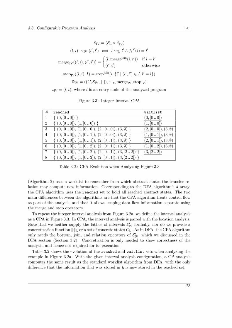
Figure 3.3.: Integer Interval CPA

# reached waitlist1 { (0, [0 .. 0]) } (0, [0 .. 0])2 { (0, [0 .. 0]), (1, [0 .. 0]) } (1, [0 .. 0])3 { (0, [0 .. 0]), (1, [0 .. 0]), (2, [0 .. 0]), (3, ∅) } (2, [0 .. 0]), (3, ∅)4 { (0, [0 .. 0]), (1, [0 .. 1]), (2, [0 .. 0]), (3, ∅) } (1, [0 .. 1]), (3, ∅)5 { (0, [0 .. 0]), (1, [0 .. 1]), (2, [0 .. 1]), (3, ∅) } (2, [0 .. 1]), (3, ∅)6 { (0, [0 .. 0]), (1, [0 .. 2]), (2, [0 .. 1]), (3, ∅) } (1, [0 .. 2]), (3, ∅)7 { (0, [0 .. 0]), (1, [0 .. 2]), (2, [0 .. 1]), (3, [2 .. 2]) } (3, [2 .. 2])8 { (0, [0 .. 0]), (1, [0 .. 2]), (2, [0 .. 1]), (3, [2 .. 2]) }

Table 3.2.: CPA Evolution when Analyzing Figure 3.3

(Algorithm 2) uses a worklist to remember from which abstract states the transfer re-lation may compute new information. Corresponding to the DFA algorithm’s A array,the CPA algorithm uses the reached set to hold all reached abstract states. The twomain differences between the algorithms are that the CPA algorithm treats control flowas part of the analysis, and that it allows keeping data flow information separate usingthe merge and stop operators.To repeat the integer interval analysis from Figure 3.2a, we define the interval analysis

as a CPA in Figure 3.3. In CPA, the interval analysis is paired with the location analysis.Note that we neither supply the lattice of intervals E ′IV formally, nor do we provide aconcretization function J·KL or a set of concrete states CL. As in DFA, the CPA algorithmonly needs the bottom, join, and relation operators of E ′IV, which we discussed in theDFA section (Section 3.2). Concretization is only needed to show correctness of theanalysis, and hence not required for its execution.Table 3.2 shows the evolution of the reached and waitlist sets when analyzing the

example in Figure 3.2a. With the given interval analysis configuration, a CP analysiscomputes the same result as the standard worklist algorithm from DFA, with the onlydifference that the information that was stored in A is now stored in the reached set.

23

3. Value Analysis

3.4. Lattices

As described in Sections 3.2 and 3.3, DFA and CPA require the space of data flowinformation to form a lattice. Lattices are partially ordered sets (see Definition 4) thatinclude a unique least upper bound (join, t) and greatest lower bound (meet, u) for anytwo elements of the set (see Definition 5). Complete lattices additionally support leastupper bound and greatest lower bound operations for subsets (see Definition 6).Figure 3.4 shows a Hasse Diagram of the powerset lattice (P({a, b}),⊆). Hasse Di-

agrams are the most common way of visualizing small lattices. Essentially, Hasse Dia-grams use the transitive reduction with an embedding such that if an element is depictedabove another, and there exists a path between the two elements, then the lower elementis smaller than the upper element. As an example, ∅ is depicted lower than {a, b} inFigure 3.4 and there exists a path between the two, therefore ∅ v {a, b}.

{a, b}

{a} {b}

∅

Figure 3.4.: Hasse Diagram of (P({a, b}),⊆)

Definition 3. Upper and Lower Bounds of Set SUB(S) = {e | ∀s ∈ S : s v e}LB(S) = {e | ∀s ∈ S : e v s}

Definition 4. Partially Ordered SetA partially ordered set is a combination of a set P and an ordering relation v: (P ×

P )− > B that fulfills the following criteria:

1. ∀a : a v a (reflexivity)

2. ∀a, b : (a v b) ∧ (b v a) =⇒ (a = b) (antisymmetry)

3. ∀a, b, c : (a v b) ∧ (b v c) =⇒ (a v c) (transitivity)

Definition 5. LatticeA lattice is a partially ordered set P that supports the binary least upper bound (t)

and greatest lower bound (u) operations (see Definition 3) as follows:∀a, b ∈ P : (a t b) ∈ P ∧ (a t b) ∈ UB({a, b}) ∧ (∀c ∈ UB({a, b}) : (a t b) v c)∀a, b ∈ P : (a u b) ∈ P ∧ (a u b) ∈ LB({a, b}) ∧ (∀c ∈ LB({a, b}) : c v (a u b))

24

3.5. Abstract Interpretation

Definition 6. Complete LatticeA lattice L is complete when it supports the least upper bound and greatest lower

bound operations on subsets (⊔,d) as follows:

∀S ⊆ L : ⊔S ∈ L ∧

⊔S ∈ UB(S) ∧ (∀c ∈ UB(S) : ⊔

S v c)∀S ⊆ L :

dS ∈ L ∧

dS ∈ LB(S) ∧ (∀c ∈ LB(S) : c v

dS)

3.5. Abstract Interpretation

Abstract interpretation (AI) is a proof framework for proving correctness of programanalyses with respect to formal semantics of the language of analyzed programs. AIwas first described by Patrick and Radhia Cousot in 1977 [36], and has been a veryactive research field since. We will first present the AI framework, and then derive therequirements for the correctness of abstract value analysis domains.With AI, one establishes a correctness relation R between an execution of program

P and its analysis. Specifically, the relation R is established between the states of theanalyzed program and their corresponding summarizations in the analysis. If a programmaps a state c1 to a state c2, then the analysis must map an abstract state a1, which is ina correctness relation with c1, to an abstract state a2, which is in a correctness relationwith c2. Figure 3.5a visualizes the correctness relation R. Here, execution of the programP maps the input state c1 to c2, denoted as P ` c1 c2. Further, the analysis of theprogram P maps a value a1 to a2, denoted as P ` a1 . a2. If the correctness relationR holds between c1 and a1 (c1 R a1), then it must also relate c2 with a2 (c2 R a2) forthe analysis to be correct. Generally, corresponds to a statement in the analyzedprogram, and . to the corresponding transfer function.Recall that each abstract domain requires its state space L to form a complete lattice.

AI requires that if s R a then ∀a′ w a : s R a′, meaning that if an abstract valueis a correct description of a concrete value, then greater values must also be a correctdescription of that value. Intuitively speaking, this requirement enforces the lattice ofabstract values to be ordered with respect to precision. Greater values are generallyless precise than smaller values. AI further requires that there exists a most precisedescription for each concrete value. With these two requirements, we can alternativelyformulate correctness via the representation function as depicted in Figure 3.5. Thisformulation of correctness makes explicit that we are allowed to approximate, usingvalues greater than the least, i.e., most precise value.For value analysis on integer programs, it is natural to accept β as β(s) = {s}, i.e.,

given a state s we return the singleton set containing s. The generated correctnessrelation R would then also accept all supersets of {s} as a correct representation. Un-fortunately, an analysis on sets of states is not feasible on infinite state systems, as nosummarization of states has taken place. This summarization can be defined by estab-lishing a Galois Connection between a precise, but possibly infeasible analysis, and anapproximative variation. The Galois Connection ensures that if the precise analysis wascorrect, then so is the approximative one.

25

3. Value Analysis

P ` c1 c2

P ` a1 a2.

R R

(a) Correctness Relation

P ` c1 c2

P ` a1 a2.

v vβ β

(b) Representation Function

Figure 3.5.: Correctness Requirements in AI

3.6. Galois Connection

A Galois Connection allows the conversion of values from one state space to anotherwithout losing correctness. It uses α to move from the precise space (concrete space) tothe less precise one (abstract space), and γ to move back. Note that α corresponds tothe abstraction function of an abstract domain, while γ corresponds to its concretizationfunction. The beauty of this approach is that Galois Connections can be chained, mean-ing we can move to more and more abstract spaces without losing correctness. Hence,AI is a modular framework, because it is not necessary to start abstractions at the mostbasic level, i.e., at the level of program states, but instead, one can abstract from anyproven point. It is, e.g., common for non-relational value analysis domains to abstractfrom integer sets, and avoid the work necessary to get to this abstraction.The formal definition of Galois Connections is given in Definition 7.

Definition 7. Galois Connection between L (concrete space) and M (abstract space),Classic Formulation

α and γ are monotone (order-preserving) functionsα : L→Mγ : M → Ll v γ(α(l))α(γ(m)) v m

Definition 7 confirms that M (abstract space) is a less precise variant of L (concretespace) in that it requires that going from the more precise L to the less precise M andback will not increase precision (γ ◦ α does not map to smaller values). Further, it alsorequires that going from the less precise M to the more precise L and back does not loseprecision (α ◦ γ does not map to greater values).Assuming a concrete state using a set of associations between program variables V ?

and integer values, and denoting an association between v and e as v 7→ e, an abstractionfrom the analysis over sets of states can be constructed as follows, where we use asuperscript # to denote an abstract state:

26

3.7. Heap Analysis

α(S) = {v 7→⋃s∈S{s(v)} | v ∈ V ?}

γ(S#) =∏v∈V ?

{v 7→ e | e ∈ S#(v)}

The abstraction function α goes through all program variables, and associates eachwith all values found under this variable in all states in S. Correspondingly, γ creates aset of associations for all values of each variable, and then uses the Cartesian Productover all resulting sets. As an example, let us abstract the set of states S = {{x 7→ 0, y 7→0}, {x 7→ 1, y 7→ 1}}:

α(S) = {x 7→ {0, 1}, y 7→ {0, 1}}The concretization is then the following:

γ(α(S)) = {{x 7→ 0, y 7→ 0}, {x 7→ 0, y 7→ 1}, {x 7→ 1, y 7→ 0}, {x 7→ 1, y 7→ 1}}We use this abstraction in our integer value analysis domain.

3.7. Heap AnalysisValue analyses are often combined with specialized analyses of the program’s heap, whichcan be considered as an association of each address, given by an integer, with a value.Since value analyzers overapproximate integers, the target of read and write operationscan, in general, not be determined. Sound integer value analyzers must overappoximatethe heap, which requires read and write operations on sets of possible addresses, whichmay overlap. Implementing a sound heap model is often challenging without concretizingthe abstract value that describes the address to read and write operations. Instead ofviewing the heap as a simple association, addressable using integers, it is common tointroduce abstract locations when objects are created. The contents of these abstractlocations is then restricted to structures of specific shapes [37, 38]. When loops thatcreated data structures cannot be shown to terminate, it must be possible to efficientlyrepresent infinite structures. Finding an efficient representation is especially challengingif no information about the shape of the represented structure is known before theanalysis. As an example, an abstract location may at first contain a hashmap, andlater on a list; hence shape analysis must be adaptive. Many shape analyses are basedon shape graphs [39], which represent which object may contain which other object.Parametric shape analysis [40] uses three valued logic to model the shape of structuresin memory. BDDStab currently does not use shape analysis as such, but uses Jakstab’sheap model instead. In Jakstab, each abstract heap location is indexable, i.e., eachabstract location consists of a region and an offset address into that region [3]. Theabstract regions are assumed to not overlap, which is unsound in general, but simplifiesthe analysis. In the default configuration, Jakstab only uses two regions to distinguishaddresses pointing to the stack from those that do not.

27

3. Value Analysis

3.8. Value Analysis Tools for Binaries

Different approaches with different soundness requirements are proposed for the analysisof machine code. Most approaches opt for improved applicability to larger programs anddo not aim for soundness. However, this does not mean that increasing precision of asound domain is not a valuable effort. It is, e.g., common to identify possible functionstart sequences in a binary and start value analysis at each of these sequences [7, 41]. Amore precise abstract domain will improve the result of analyzers that use this approach.

Possibly the best-known commercial tool is GrammaTech’s CodeSurfer/x86 [41], whichassumes that the code it analyzes has a clear separation of data and code, does notmodify itself, and adheres to stack discipline. Hence it may not be suited to analyzeexecutables that are designed to hide their behavior. However, CodeSurfer/x86 doesuse value analysis (k-set analysis) in combination with abstract locations, determined inpart using IDAPro’s heuristics, to compute possible targets for dynamic jumps.

The Jakstab framework [3] uses the SSL intermediate language [42] to support theformulation of analyses. For the analyses, it makes use of the CPA formulation, whichmeans that approaches known from software model checking as well as classic DFAand combinations thereof are implementable. Jakstab provides several value analysesto resolve jump targets, such as k-set, interval, and sign-agnostic interval domains [43].We extend Jakstab with an unrestricted set domain with abstract values represented byBDDs.

Another analysis framework for the analysis of executables is the binary analysisplatform (BAP) [44]. BAP’s focus is on providing a well-specified intermediate languageas a common grounds for implementing further analyses. BAP uses special instructionsfor indirect jumps, which may be resolved using value set analysis [45]. However, itseems that the main focus of BAP is on working with code in its intermediate languageBIL, and not on soundly lifting machine code to BIL.

Bitblaze [46], which is in part a predecessor to BAP, combines static and dynamicanalyses to increase precision. Its dynamic analysis part is based on the Qemu [47]emulator.

Another comprehensive effort is the Bincoa framework [48], which also formulates acommon model for the analysis of executables. Its tool set consists of Osmose [49], a testdata generation tool for binaries, Insight [50], a tool that supports lifting and analysisincluding value analysis, and TraceAnalyzer [51], a tool that uses value analysis andrefinement of VDs that are used in dynamic jumps and have been overapproximated to>.

All of the above-mentioned tools that use value analysis, approximate VDs using eithera form of intervals, or k-sets, or a combination thereof. In difference, with BDDStab, weprovide a value analysis that does neither enforce convexity nor is restricted to a specifictype of non-convexity.

28

3.9. Binary Decision Diagrams

3.9. Binary Decision Diagrams

Binary Decision Diagrams (BDD) [52, 53, 54] are an efficient graph representation forBoolean functions, i.e, functions of the type Bn → B, that consist of decision nodesand terminal nodes. Decision nodes have two outgoing edges to sub-BDDs and carry aslabel a variable that determines which edge must be followed during evaluation of theBDD. The terminal node’s label determines the result of the function. Usually, BDDsare based on the Shannon Decomposition, shown in Definition 8, where xk is used aslabel in a decision node, and the BDD representation of fxk

and f¬xkare used as targets

of the decision node’s edges. When repeated application of Shannon Decomposition andconstruction of decision nodes yields a Boolean constant, then this constant is used aslabel in a terminal node. One early form of BDD is the free BDD (FBDD) [55], whichenforces that no path within the BDD may contain two decision nodes with the samelabel, in order to avoid reading the same input more than once.

Definition 8. Shannon DecompositionAssuming an n-ary Boolean function f(x1, . . . , xn) = f(x), the positive and negative

cofactors of f are defined asfxk

(x) = f(x1, . . . , xk−1, 1, xk+1, . . . , xn−1)andf¬xk

(x) = f(x1, . . . , xk−1, 0, xk+1, . . . , xn−1).

Any n-ary Boolean function can be decomposed into two functions of arity n − 1 bythe Shannon Decomposition:f(x) = (xk ∧ fxk

(x)) ∨ (¬xk ∧ f¬xk(x))

In the following, we will visualize decision nodes using a circular node, labeled withthe corresponding variable. If this variable is true, then evaluation must continue at thesub-BDD reachable by traversing the solid edge, and otherwise it must continue at thesub-BDD reachable using the dashed edge. Terminals are represented using rectangularnodes, labeled with the Boolean constant they represent. In text form, we use 1 for atrue terminal, and 0 for a false terminal. The graphs in Figure 3.6 represent Booleanand.

x1

x2

01

(a) BDD 1

x2

x1

01

(b) BDD 2

x1

x2 x2

10

(c) BDD 3

x1

x2 0

1 0

(d) BDD 4

Figure 3.6.: Equivalent BDDs Representing and

29

3. Value Analysis

The core advantage of BDDs is that they support canonicity, meaning that any twoequivalent Boolean functions have the same BDD representation, which allows equiva-lence checking in O(1), and in turn enables a systematic optimization of functions onBDDs using caches [56]. Since the BDDs in Figure 3.6 represent the same Boolean func-tion, but use different graphs, it is clear that some restrictions are missing to enforcecanonicity. The first restriction is to define a total order on all variables, and enforcethat the encountered labels on all decision nodes are strictly ascending along all pathsof the BDD. BDDs that fulfill this restriction are called ordered (OBDD) [54]. If wechoose the order to include x1 < x2, then BDD 2 is disallowed. To disallow BDDs 3 and4, only BDDs that have been fully reduced with the following two rules are allowed.

1. When both successors of a decision node are the same BDD, delete the node andredirect its incoming edges to the successor.

2. When a BDD contains two equal sub-BDDs, delete one and redirect its incomingedge to the other.

Since the right x2 node in BDD 3 can be removed using Rule 1, and one of the 0sub-BDDs in BDD 4 is redundant and can therefore removed by Rule 2, both BDDsare forbidden, leaving only BDD 1. OBDDs that are unchanged by both rules suchas BDD 1 are called reduced OBDD (ROBDD) [54, 56] and support canonicity. SinceROBDDs are the most common BDD structure, we will use the terms BDD and ROBDDsynonymously in the remainder of this thesis.There has been extensive research in optimizing the size of BDDs by optimizing the

variable order [57, 58, 59]. Unfortunately, ordering optimizations depend on heuristics,and reordering BDDs is NP-complete [60]. Further, most operations on BDDs requireall operand BDDs to respect the same, or a compatible, ordering, which means that itis unlikely that a chosen ordering is near optimal for all BDDs.Another optimization is the complementable edges extension [61], which makes the

interpretation of the terminal’s label path-dependent, whereby it allows up to twice asmany BDDs to be shared in memory. With this extension, a BDD and its complementshare the same structure, and differ only in one Boolean that is stored outside of theshared BDD part. Consider the BDD in Figure 3.7, which represents a ∧ ¬b, where aand b are ordered as follows: a > b.

BDDs with complementable edges only require one terminal node, i.e., 1 . With com-plemented edges, the incoming edges to a node can signal that the result of the evaluationmust be complemented, hence the interpretation of the 1 node is path-dependent. Werepresent edges that signal complementation of their targets using a circle in the mid-dle of them, while edges that do not signal complementation are visualized without thecircle. To allow complementing of entire BDDs, a dangling incoming edge to the BDDis added. This edge is not part of the BDD structure itself, and is therefore not shared.Hence, a BDD and its complement are shared and the number of unique BDDs is halved.The interpretation of a BDD with complement edges is as follows: Paths that contain

an even number of complement edges lead to 1 , paths that contain an odd number of

30

3.9. Binary Decision Diagrams

a

b

1

Figure 3.7.: BDD Representing a ∧ ¬b

x x x x

x x x x

Figure 3.8.: Complemented Edges Conflicts

complement edges lead to 0 . The only path with an even number of complementations inthe BDD from Figure 3.7 is a = 1, b = 0. All other paths have only the complementationfrom the dangling edge and will therefore lead to 0 .

There is, however, one restriction missing to make complemented edges canonical.Consider Figure 3.8, which contains pairs of semantically equivalent BDDs with differingstructure. To restore canonicity to BDDs with complemented edges, it is forbidden tohave a solid complement edge of the internal nodes. Consequently, whenever a node isto be constructed with a solid complement edge, the complement information on thedangling edge as well as the one on the unset edge are inverted instead.An alternative formulation of BDDs can be derived from the Davio decomposition,

provided in Definition 9, instead of the classic Shannon decomposition. Using either thepositive or negative Davio Decomposition exclusively results in the functional decisiondiagrams, named pFDD for positive decomposition and nFDD for negative decomposi-tion [62]. It is also possible to use positive or negative decomposition per variable, whichresults in general FDDs [63].Similarly to FDDs, one can also allow using Shannon, and positive and negative Davio

Decomposition per variable. Decision diagrams constructed with all three decomposition

31

3. Value Analysis

types are called Kronecker functional decision diagrams (KFDD) [64].

Definition 9. Davio DecompositionWe define the Boolean derivation of a function f(x1, . . . , xn) as

∂f∂xk

= fxk(x)⊕ f¬xk

(x).

Any Boolean function with n > 0 inputs f(x0, . . . , xn−1) can be decomposed in twoways into sub-functions with n− 1 inputs:

1. Positive decomposition: f = f¬xk⊕ xk ∧ ∂f

∂xk

2. Negative decomposition: f = fxk⊕ ¬xk ∧ ∂f

∂xk

Apart from introducing alternative decompositions, other techniques have been re-searched to reduce the size of the decision diagrams for specific configurations. Whensolving combinatorial problems, it is often desirable to manipulate subsets of the pow-erset of an n-element set. Those subsets, commonly called combinations, can be rep-resented by BDDs by assigning one input variable to each combination, and storingthe indicator function of a set of combinations in a BDD. When n is large, there existextremely many input variables to the indicator function, hence the reduction rule ofBDDs that removes decision nodes must be efficient. It is common for combination setsto be sparse, i.e., combination sets usually are small compared to their maximum size.Therefore, if the indicator function of common combination sets is true, then it is likelythat most inputs are false. Representing such function in a classic BDD would lead tomany decision nodes where the true successor edge points to 0 , meaning the decisionnode cannot be deleted. To have a more efficient representation in this application,Minato introduced zero suppressed BDDs (ZDD) [65], which are classic BDDs basedon Shannon’s Decomposition with a modified reduction rule. Instead of eliminating adecision node exactly when both its successors are the same node, in ZDDs, decisionnodes are removed if their true edge points to 0 , leading to an efficient representationfor sparse combination sets.A common generalization of classic BDDs is to relax the requirement that leaves

contain a Boolean, and instead allow values from another finite domain. In verification,this domain of values is often a subset of integral numbers. Such decision diagrams arecalled multi-terminal BDDs (MTBDDs) [66]. A special form of MTBDDs are algebraicBDDs (ADDs), which are MTBDDs that are specialized for algebraic applications [67].Yet another way in which decision diagrams differ from classic BDDs are attribute

edges, where edges carry information other than whether they correspond to a true orfalse decision. An optimization to MTBDDs with integer leaves are edge-valued BDDs(EVBDDs) [68], which attribute the BDD edges with integer offsets to improve sharing.Such edge weights can also be generalized to factors, where the edge attributes along apath to a leaf are not added to the leaf’s integer, but multiplied instead.

32

3.9. Binary Decision Diagrams

Another decision diagram, designed for the verification of timed automata, are dif-ference decision diagrams (DDD) [69], which represent a Boolean logic over inequalitiesof the form x − y ≤ c. Modified algorithms from classic BDDs support unification andintersection of the non-convex and relational space that DDDs represent.Numeric decision diagrams (NDDs) [70] are designed with a similar goal as DDDs,

namely the verification of timed automata. Specifically, NDDs target the representationof discrete and dense clock variables, the latter by discretization. Essentially, NDDsrepresent bitvectors that may be built from the concatenation of bitvectors that representvariables in the analyzed automaton.For our BDD-based integer set implementation, we introduce a variant of ROBDDs

with complement edges that is optimized for representing Boolean functions with fewinput variables. Our BDDs do not label the decision nodes with their correspondingvariable, which enables sharing of BDDs that are structurally equivalent but representdifferent functions.

33

4. BDDStab Library

The BDDStab library enables the definition of integer value analysis domains for data-flow-based analysis tools using abstract interpretation. It takes its name from its usein the binary analysis platform Jakstab via the BDDStab Jakstab adapter. In thisapplication, the BDDStab library provides the heavy lifting, i.e., the representation ofabstract integer values and the transfer functions. By using maximally shared BDDs torepresent abstract values, the BDDStab library minimizes the memory consumption ofthe many abstract states that must be stored during analysis. The right side of Figure4.5 shows the BDD representation of the integer set {1, 2}. Each path of the BDD thatterminates in 1 represents included integers, in this case 1 for the grey path, whichencodes 0 ∗ 21 + 1 ∗ 20 since the decision node corresponding to 21 is false and the nodecorresponding to 20 is true, and 2 for the orange path, which encodes 1 ∗ 21 + 0 ∗ 20.Complement edges, as introduced in Section 3.9, allow the same BDD to be representedby just two nodes. Further savings are achieved if sub-ranges covering powers of two,i.e., [2n .. 2n+m − 1] are either included or excluded from the represented set, becausethen, entire sub-BDDs are set to 1 or 0 respectively. In difference to most other valueanalysis domains such as the interval abstract domain, the BDDStab library does notrequire convexity and provides precise transfer functions on the bit level. Table 4.1 givesan overview of the provided functions and in case of transfer functions, categorizes theirapproximation behavior, where we use P for precise, A for approximating, and an emptycell if the method is not a transfer function. We consider an n-ary transfer function of aconcrete operator as precise exactly when it produces exactly the set of all combinationsof the n input sets with the operator applied. A transfer function ◦# is precise for thebinary operator ◦ exactly when A ◦# B = {a ◦ b | a ∈ A, b ∈ B}.

In this chapter, we describe our BDD representation in detail and provide implemen-tations for all common transfer functions.

4.1. BDD Structure

To optimize for the operations that we use in BDDStab, we use a modified BDD struc-ture. We base our structure on reduced ordered binary decision diagrams with comple-mentable edges, but modify it to improve sharing. Specifically, we do not store variablenames in each decision node’s label as would be done using traditional BDDs, and makethe correspondence between a decision node and its variable dependent on the depthof the decision node in the BDD. Additionally, we add set cardinality, i.e., determiningthe number of represented concrete elements, in O(1) by precomputing values duringeach construction of a decision node. This precomputation needs to be adapted to workso that it is dependent on the BDD depth, because when each decision node’s label isdetermined by its depth, the same BDD, rooted at different depths, may represent setsof different sizes. As an example, a 1 node can represent varyingly many elements,depending on its depth in a BDD.

35

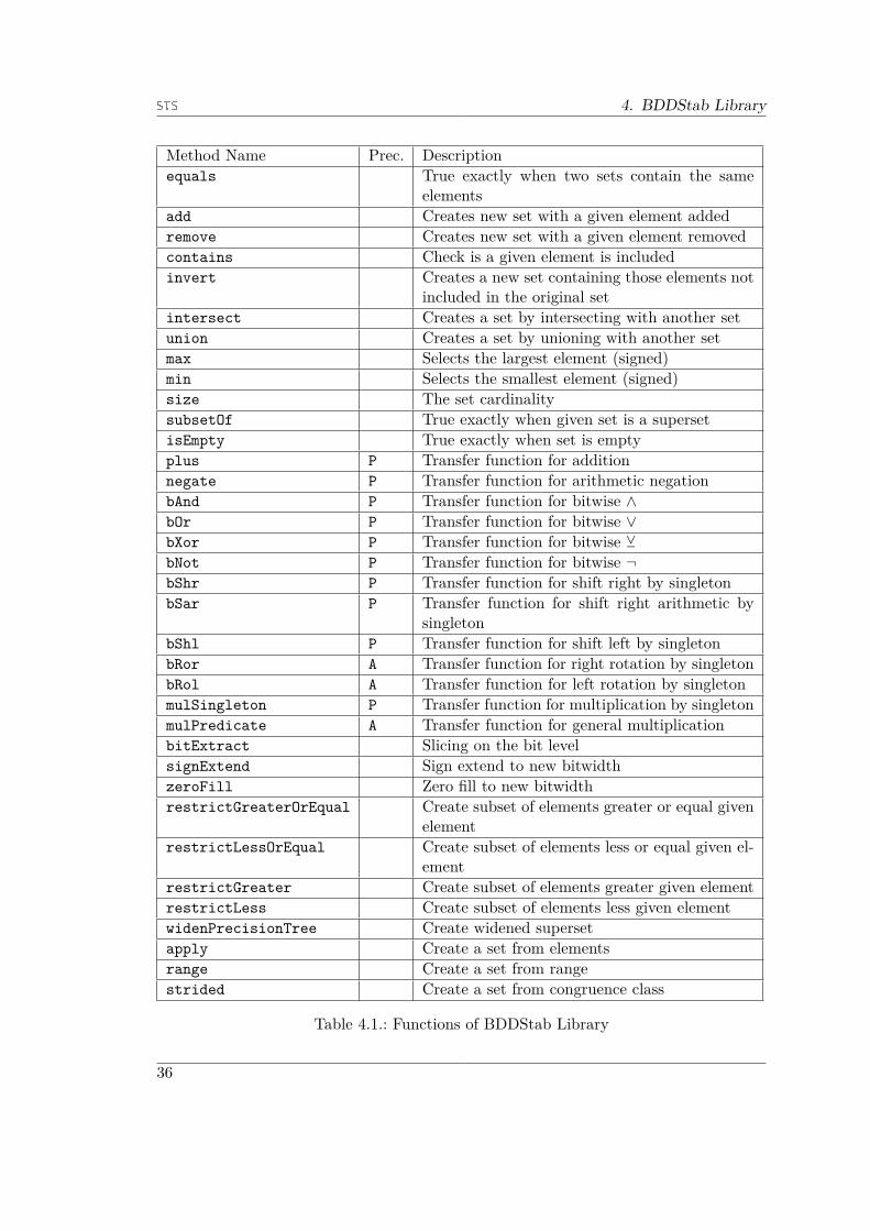
4. BDDStab Library

Method Name Prec. Descriptionequals True exactly when two sets contain the same

elementsadd Creates new set with a given element addedremove Creates new set with a given element removedcontains Check is a given element is includedinvert Creates a new set containing those elements not

included in the original setintersect Creates a set by intersecting with another setunion Creates a set by unioning with another setmax Selects the largest element (signed)min Selects the smallest element (signed)size The set cardinalitysubsetOf True exactly when given set is a supersetisEmpty True exactly when set is emptyplus P Transfer function for additionnegate P Transfer function for arithmetic negationbAnd P Transfer function for bitwise ∧bOr P Transfer function for bitwise ∨bXor P Transfer function for bitwise YbNot P Transfer function for bitwise ¬bShr P Transfer function for shift right by singletonbSar P Transfer function for shift right arithmetic by

singletonbShl P Transfer function for shift left by singletonbRor A Transfer function for right rotation by singletonbRol A Transfer function for left rotation by singletonmulSingleton P Transfer function for multiplication by singletonmulPredicate A Transfer function for general multiplicationbitExtract Slicing on the bit levelsignExtend Sign extend to new bitwidthzeroFill Zero fill to new bitwidthrestrictGreaterOrEqual Create subset of elements greater or equal given

elementrestrictLessOrEqual Create subset of elements less or equal given el-

ementrestrictGreater Create subset of elements greater given elementrestrictLess Create subset of elements less given elementwidenPrecisionTree Create widened supersetapply Create a set from elementsrange Create a set from rangestrided Create a set from congruence class

Table 4.1.: Functions of BDDStab Library

36

4.1. BDD Structure

4.1.1. Labelless NodesDuring analysis, a value analyzer, such as the BDDStab adapter to Jakstab (Section 5),produces at least one abstract state per reachable program location. Lifted versions oflow-level code, such as executables, tend to increase the number of program locations,as each effect of an instruction is made explicit. Each abstract state in turn is composedof one abstract value per storage location, of which there may exist as many as there areheap entries. Therefore, a value analyzer tends to store extremely many abstract values,the collection of which must therefore be size-efficient. We therefore decide to optimizethe well-known BDD structure to improve sharing. Additionally, improved sharing alsoallows for improved memoizing of functions. Our labelless nodes modification of BDDsdoes not store variable names in the decision nodes, but makes the decision node’svariable dependent on the depth of the decision node in the BDD itself. The advantageof this modification is that two structurally equivalent BDDs can be shared, even if theyrepresent different boolean functions. Consider the BDDs in Figure 4.1. The rectangularnode that points to the BDDs contains the BDD ordering and is headed by the namedBoolean function. The top-most marked (grey) decision node for fa decides on variablex2, as it is the second node on all BDD paths. Because this decision node points to 1for the true successor and 0 for the false successor, it represents the function x2. In fb,the same marked structure represents the function x1, as the top-most marked decisionnode is the first on all paths in this BDD. Since all three marked sub-BDDs in Figure4.1 are structurally equivalent, it is possible to share them as done in the right-hand sideforest. To make the depth of a node determine its label, we modify reduction Rule 1 asfollows:

1. When both successors of a decision node are the same terminal, delete the nodeand redirect its incoming edges to the terminal.

The disadvantage of this approach is that the reduction rules of traditional BDDsmust be changed to allow a clear correspondence between decision node and its placein the BDD ordering. There may not be any gaps, meaning variables in the orderingthat have no corresponding decision node, between any two decision nodes in a labellessBDD. Only nodes with false and true successor pointing to the same terminal nodemay be deleted. Therefore, a labelless BDD such as the one representing fc may havemore nodes than one with explicit labels within its decision nodes. In this BDD, theroot node would traditionally have been removed, as both successors point to the sameBDD. However, with labelless nodes, this is not possible as removal would change theinterpretation of the top-most marked decision node. On the upside, none of the markedsub-BDDs could have been shared in a traditional BDD structure, but all of them areshared with labelless nodes.Since equivalence check on BDDs is in O(1), it is possible to skip redundant decision

nodes in O(1) during BDD operations. The penalty in the efficiency of the algorithmsthat has to be expected therefore depends on the maximal number of variables in theordering. Since this number of variables in the ordering is bounded by the widest in-teger type to be analyzed, no huge negative impact must be expected. As an example,

37

4. BDDStab Library

π: x1 < x2

fa: x1 ∨ x2

1 0

π: x1 < x2

fb: x1

1 0

π: x2 < x1

fc: x1

1 0

π: x2 < x1

fc: x1π: x1 < x2

fa: x1 ∨ x2

π: x1 < x2

fb: x1

1 0

Figure 4.1.: Improved Sharing with Labelless Nodes

the BDDStab Jakstab adapter uses at most 64 variables in the ordering to adequatelyrepresent 32 bit integers after multiplication.

4.1.2. Structural Induction

To prove correctness of our algorithms on BDDs, we will use proof by induction. Morespecifically, we use structural induction, as we operate on trees rather than naturalnumbers. Assuming a property P that is to be shown for arbitrary trees, structuralinduction operates by showing P for the basic elements of the tree, i.e., the leaves, andthen showing that if P holds for the sub-trees, it also holds for a tree constructed fromthose sub-trees. Formally, structural induction on BDDs for an arbitrary property P istherefore:Base Cases: P (0), P (1)Inductive Case: ∀X,Y : P (X) ∧ P (Y ) =⇒ P ((X ◦ Y ))It is important for an induction scheme to be complete, meaning that if base case and

inductive case are proven, then it must be possible to construct P for arbitrary BDDs.

Induction Scheme for Cartesian Product BDD Algorithms

Interestingly, our algorithms for binary transfer functions, such as addition, operate ontwo BDDs and their correctness must therefore be encoded in a binary property, i.e., ofthe form P (X,Y ) instead of P (X). Possibly the first idea that one might have is to usethe Cartesian product of the base cases and extend the inductive step as follows:

Scheme 1. Incomplete Induction Scheme for Cartesian Product Fashion AlgorithmsBase Cases: P (0 , 0)

P (0 , 1),P (1 , 0),P (1 , 1)

Inductive Case: ∀A,B,C,D : P (A,B) ∧ P (C,D) =⇒ P ((A ◦ B), (C ◦ D))

38

4.1. BDD Structure

This scheme, however, is not complete. Consider the BDD in Figure 4.2.

1

0 1

1 0

Figure 4.2.: BDDs not Covered by Induction Scheme 1

This tuple of BDDs is constructed using (((0 ◦ 1) ◦ 1), (1 ◦ 0)). To concludeP (((0 ◦ 1) ◦ 1), (1 ◦ 0)), it is necessary to have P ((0 ◦ 1), 1) and P (1 , 0). How-ever, P ((0 ◦ 1), 1) cannot be constructed since there exists no way to construct a non-terminal BDD on one side and a terminal on the other. Hence, P cannot be establishedusing only the base and inductive cases for the BDD in Figure 4.2, because the inductivecase forces the node constructor in both arguments to P , which is why only pairs ofBDDs with the same depth are covered by this induction scheme. Furthermore, ouralgorithms proceed in a Cartesian product fashion, and require correct sub-results notonly for P (A,B) and P (C,D) but also for P (A,D) and P (B,C).

We therefore propose the following induction scheme:

Scheme 2. Induction Scheme for Cartesian Product Fashion AlgorithmsBase Cases: ∀B : P (0 , B),

∀B : P (1 , B),∀A : P (A, 0),∀A : P (A, 1)

Inductive Case: ∀A,B,C,D : P (A,C) ∧ P (A,D) ∧ P (B,C) ∧ P (B,D)=⇒ P ((A ◦ B), (C ◦ D))

With this induction scheme, it is possible to derive P for the example BDD in Figure4.2 as follows:

P ((0 ◦ 1), 1) ∧ P ((0 ◦ 1), 0) ∧ P (1 , 1) ∧ P (1 , 0)=⇒ P (((0 ◦ 1) ◦ 1), (1 ◦ 0))

All P s in the antecedent (induction hypothesis) of this derivation are covered by basecases, hence P can be derived for the whole tuple of BDDs.

4.1.3. Set Cardinality in O(1)When operating on sets, one often wants to know the cardinality, i.e., how many ele-ments are included. With the BDD-based set encoding, the corresponding operation issatisfiability count, which essentially searches for paths to true terminals in the BDD.Each discovered path to 1 represents 2n satisfiable variable valuations, where n is the

39

4. BDDStab Library

number of variables without a corresponding decision node. Unfortunately, this simplealgorithm requires full traversal of the BDD, which should be avoided as the operationis often executed, e.g., to judge precision loss in widening, determine if a precise heapoperation would be too expensive as there are too many possible addresses, consideringwhether printing the set to the screen should list all elements, or to produce a goodapproximation in operations such as multiplication. For traditional BDDs, it is possibleto compute and store the satisfiability count whenever a BDD is constructed from twoother BDDs by taking the precomputed satisfiability count from each input BDD, mul-tiplying them by 2n, where n is the size of the gap between the new node and the rootnode of the corresponding input BDDs, and adding the result. However, since labellessnodes do not carry variables, this simple algorithm cannot be used as the number ofsatisfiable valuations of a labelless BDD depends on the layer it is rooted in. The solu-tion is to cache not the total number of satisfiable variable valuations, but the minimalnumber and height instead. Consider the two left-most BDDs in Figure 4.1. The markedsub-BDD contains 20 satisfiable variable valuations in fa, because there is no variableleft in the ordering at the decision node’s successors, and 21 such paths in fb, becausethere is one variable left in the ordering at the decision node’s successors. The differencebetween the two interpretations is that one is rooted at a higher layer in the orderingthan the other.A key insight is that if a BDD has height h, then each terminal at depth d represents at

least 2h−d = c satisfiable variable valuations. As we have learned from the example, theexact number of satisfiable variable valuations represented by each 1 depends addition-ally on where the corresponding BDD is rooted in the ordering. Assuming the number ofelements in the ordering to be n, the number of variables that are not referenced within agiven BDD of height h is n− h. Since these variables multiply the number of satisfiablevariable valuations by 2 each, the exact number of satisfiable variable valuations canbe computed by multiplying the minimal number of satisfiable variable valuations with2n−h. The parameters c and h depend only on the structure of a given BDD, and not onits interpretation. Hence, it is safe to cache the two parameters for each decision node,even in the presence of sharing. If n is known, which is the case in the BDDStab library,then the parameters c and h are sufficient in computing the exact satisfiability countusing c ∗ 2n−h.To not negatively affect BDD performance, the computation of the parameters c and h

for a new decision node must be in O(1). The parameters c and h for 0 and 1 are c = 0,h = 0, and c = 1, h = 0 respectively. Given two BDDs s and u, with s.h, u.h, s.c, and u.cdenoting their height and minimum satisfiability count respectively, then the new heightof a node (s ◦ u) is max(s.h, u.h) + 1 = (s ◦ u).h, the computation of which is indeed inO(1). Computing (s ◦ u).c from s.h, s.c, u.h, and u.c cannot be done by simply addings.c and u.c because the minimum number of input variables, referenced by (s ◦ u), isdetermined by its height, which in turn is computed using the maximum height of sand u. Within (s ◦ u), the minimum number of referenced input variables of s and u ismax(s.h, u.h). If s.h ≤ u.h, we therefore compute (s ◦ u).c = s.c ∗ 2|s.h−u.h| + u.c, whichadjusts the minimum satisfiability count of s to the depth of u. Similarly if u.h ≤ s.h,

40

4.1. BDD Structure

satnaive(n, 1) = 2nsatnaive(n, 0) = 0satnaive(n, (s ◦ u)) = satnaive(n− 1, s) + satnaive(n− 1, u)

Figure 4.3.: Satcount Naive

we compute (s ◦ u).c = u.c ∗ 2|s.h−u.h| + s.c. In both cases, the computation is in O(1).As an example, consider the creation of the unmarked node of fa. The height of the

newly computed BDD is 2, the minimum satisfiability count is 3, while the height of themarked sub-BDD A is 1 and its minimum satisfiability count is 1. With A = (1 ◦ 0),i.e., the marked sub-BDD, the corresponding computation of the minimum satisfiabilitycount for fa is as follows:

A.c = 1 .c ∗ 21 .h−0 .h + 0 .c = 1 .c+ 0 .c = 1

(1 ◦ A).c = 1 .c ∗ 21 .h−A.h +A.c = 1 ∗ 21 + 1 = 3

Since the number of input variables n is known for each BDD r, and the height andminimum satisfiability count are cached, we define our set cardinality as:

sat(n, r) = 2n−r.h ∗ r.c

The O(1) BDD-set cardinality has been implemented and evaluated as part of a bach-elor thesis [71].In the following, we prove equivalence between the non-naive method of computing the

number of satisfiable variable valuations as outlined above, and a naive implementationas given in Figure 4.3. This naive algorithm takes the number of input variables to therepresented function and a corresponding BDD, and recurses the BDD until it reachesa terminal node. During this recursion, it keeps track of the number of traversed inputvariables, and is thereby able to compute the number of unique paths to 1 , representedby a 1 .Figure 4.4 proves equivalence between the naive and the non-naive satisfiability count

algorithms. The proofs of the two base cases (4.1, 4.2) are trivial. The value of r.c is0 for a terminal false node and 1 for a terminal true node. The proof for the inductivecase (4.3) is slightly more involved. Since the construction of r.h for a new node r usesthe max function and the construction of r.c takes the absolute value of an expression,we use case distinction in our proof for r1.h ≤ r2.h and r1.h > r2.h. Note that for thefirst case, we have (r1 ◦ r2).h = r2.h + 1 and (r1 ◦ r2).c = r2.c + 2r2.h−r1.h ∗ r1.c, sincewe take the maximum height plus one and have to adjust the minimum count of r1 tothe depth of r2.

41

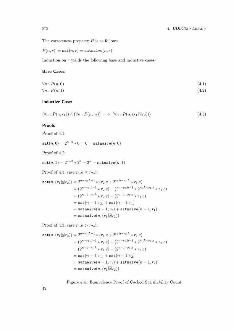
4. BDDStab Library

The correctness property P is as follows:

P (n, r) := sat(n, r) = satnaive(n, r)

Induction on r yields the following base and inductive cases.

Base Cases:

∀n : P (n, 0) (4.1)∀n : P (n, 1) (4.2)

Inductive Case:

(∀n : P (n, r1)) ∧ (∀n : P (n, r2)) =⇒ (∀n : P (n, (r1 ◦ r2))) (4.3)

Proofs

Proof of 4.1:

sat(n, 0) = 2n−0 ∗ 0 = 0 = satnaive(n, 0)

Proof of 4.2:

sat(n, 1) = 2n−0 ∗ 20 = 2n = satnaive(n, 1)

Proof of 4.3, case r1.h ≤ r2.h:

sat(n, (r1 ◦ r2)) = 2n−r2.h−1 ∗ (r2.c+ 2r2.h−r1.h ∗ r1.c)= (2n−r2.h−1 ∗ r2.c) + (2n−r2.h−1 ∗ 2r2.h−r1.h ∗ r1.c)= (2n−1−r2.h ∗ r2.c) + (2n−1−r1.h ∗ r1.c)= sat(n− 1, r2) + sat(n− 1, r1)= satnaive(n− 1, r2) + satnaive(n− 1, r1)= satnaive(n, (r1 ◦ r2))

Proof of 4.3, case r1.h > r2.h:

sat(n, (r1 ◦ r2)) = 2n−r1.h−1 ∗ (r1.c+ 2r1.h−r2.h ∗ r2.c)= (2n−r1.h−1 ∗ r1.c) + (2n−r1.h−1 ∗ 2r1.h−r2.h ∗ r2.c)= (2n−1−r1.h ∗ r1.c) + (2n−1−r2.h ∗ r2.c)= sat(n− 1, r1) + sat(n− 1, r2)= satnaive(n− 1, r1) + satnaive(n− 1, r2)= satnaive(n, (r1 ◦ r2))

Figure 4.4.: Equivalence Proof of Cached Satisfiability Count42

4.2. Representing Integer Sets

4.2. Representing Integer Sets

As outlined before, we use our BDD structure to represent integer sets in BDDStab.Traditionally, BDDs are a data structure to represent Boolean functions. Many struc-tures can be encoded as Boolean functions and can therefore also be stored in a BDD.As is customary, our encoding of integer sets uses the two’s complement conversion ofintegers to bitvectors, of which each bit is treated as an input to the Boolean function,represented by the BDD. This Boolean function returns true exactly when the corre-sponding bitvector and, therefore, the integer is included. In other words, we take theindicator function for the n-bit integer set, convert it to a Boolean function of the form{0, 1}n → {0, 1}, and represent that function using a BDD. Reduction of the resultingBDDs requires an ordering to be defined on its input variables, which we discuss in thenext subsection.

Ordering

Theoretically, one could choose any permutation of the n input variables to representn-bit integer sets. However, we also have to consider that we want to execute operationson the BDDs and these operation’s efficiency depends on the variable ordering. Thereare two natural choices for the variable ordering: Most significant bit (MSB) to leastsignificant bit (LSB) and LSB to MSB. LSB to MSB ordering, meaning the LSB is thebit associated with the root node of the BDD, simplifies the definition of the additionoperation, since the carry bit distributes from LSB to MSB and so does each path in aBDD with LSB to MSB ordering. However, with this ordering, two consecutive integersare not close with respect to the BDD structure. Consider Figure 4.5, which depictstwo non-reduced BDDs representing the integer set {0, 1}, the one with LSB to MSBordering on the left, and the one with MSB to LSB ordering on the right. Even thoughthe represented numbers in the set are consecutive, the paths on the left-hand side BDDare not, meaning the terminal node for one number could be far to the left and theterminal node for the other number could be far to the right even though the numbersare consecutive. In difference, in the BDD on the right-hand side, two numerically closeunsigned integers will have paths that are close to each other. In the MSB to LSBrepresentation, it is therefore more likely that a range of integers will have an efficientBDD representation as it is likely that reduction is able to remove nodes where bothsuccessors are the true terminal. Figure 4.6 illustrates this fact. Whenever an interval isto be represented in a BDD with MSB to LSB ordering, there are essentially two paths,one corresponding to the lower bound and one corresponding to the upper bound, whichborder an area of included integers. In other words, the successors of the nodes on thosepaths that point inwards are set to the true terminal, and the successors pointing tothe outside are set to the false terminal. Again, it is likely that there exist nodes thatcan be removed because both successors point to the terminal true in the inside (green)area. Since it is known that convex shapes, i.e., intervals in the non-relational case, arecommon during the analysis of software, we choose the MSB to LSB ordering to have amore efficient representation and conversion to and from intervals.

43

4. BDDStab Library

20

21 21

0 1 0 1

Xa = {0, 1} 21

20 20

0 1 1 0

Xb = {1, 2}

Figure 4.5.: Variable Ordering Options

2MSB

1

0 0

Figure 4.6.: Interval Conversion of [2 .. 7] with MSB to LSB Ordering

4.3. Conversion AlgorithmsIn this section, we present algorithms to create BDD-based integer sets from well-knownabstractions, namely singleton integers, intervals, and strided intervals. Additionally,we provide an approximating algorithm to convert a BDD-based integer set to a setof intervals, which can be used to synthesize transfer functions on BDD-based integersets from their corresponding counterparts in the interval abstract domain. Most of thealgorithms are recursive, and many count their recursion depth in a parameter, which hasto be set to 0 or a constant at the outer-most recursion. To avoid the explicit handlingof this parameter in the presentation of an algorithm, we use named parameters thatmust be associated with a default value and must be set by name should this defaultvalue be overwritten. Note that to avoid ambiguities, no regular parameters are allowedafter a named parameter in the parameter lists. The parameter d in Algorithm 3 is sucha named parameter, denoted using = in the algorithm’s parameter list. Its default valueis n− 1, and it is explicitly set to d− 1 in the recursive calls to fromNumber.

4.3.1. Configurable BDD Construction from Singletons

Algorithm 3 takes a singleton integer, and creates a BDD by creating the path describedby the corresponding bitvector. This algorithm is configurable in the BDDs it placesoutside of the path described by the given integer, and by the terminal node it places

44

4.3. Conversion Algorithms

at the end of the path. It can therefore be used to convert the unsigned n-bit integeri not only to a singleton BDD set {i} using fromNumber(i, 0, 0, 1), but also to aBDD-based integer set {e | e ≥ i}{n} using fromNumber(i, 1, 0, 0). A set with allintegers smaller than i can be created similarly.

Algorithm fromNumber(a, S, U, T, d = n− 1) isInput: n-bit integer a, depth d, set BDD S, unset BDD U , terminal BDD TResult: BDD with path given by a, terminated by T , all true successors

leaving path to S, all false successors leaving path to U1 if d < 0 then return T2 if a{d} then3 return (fromNumber(a, S, U, T, d = d− 1) ◦ U)

else4 return (S ◦ fromNumber(a, S, U, T, d = d− 1))

endend

Algorithm 3: Configurable Construction from Integer to BDD

As an example, let us use Algorithm 3 to create the set of all 3-bit unsigned integersgreater or equal than 2. From Figure 4.6, we know that the corresponding BDD mustcontain the path corresponding to the bitvector of 2, i.e., 010, and all BDDs to the leftor greater side must be set to 1 and all BDDs to the right or smaller side must be setto 0 . This BDD can be constructed using fromNumber(2, 1, 0, 1, d = 2):

fromNumber(2, 1, 0, 1, d = 2) =(1 ◦ fromNumber(2, 1, 0, 1, d = 1)) =(1 ◦ (fromNumber(2, 1, 0, 1, d = 0) ◦ 0)) =(1 ◦ ((1 ◦ fromNumber(2, 1, 0, 1, d = −1)) ◦ 0)) =(1 ◦ ((1 ◦ 1) ◦ 0)) =(1 ◦ (1 ◦ 0))

The resulting BDD is true if the 22 bit is set or if the 21 bit is set, otherwise it is false.This represents exactly the set of all 3-bit integers greater than 2.

4.3.2. BDD Creation from Standard Intervals

Algorithm 4 performs the conversion from an integer interval to a BDD-based integerset. The algorithm takes two (d + 1)-bit unsigned integers a and b, with a ≤ b, andcreates a BDD-based integer set {i | a ≤ i ≤ b}. Even though this algorithm operates onunsigned integers only, it is easily possible to use it for signed integers, by calling it oncefor all negative, and once for all positive integers and union the results. The algorithmuses fromNumber to create a set of all unsigned integers smaller than b and a set of allunsigned integers greater than a. The desired result is then the intersection of these twoBDDs, which is computed using the well known if-then-else algorithm (ite) [56].

45

4. BDDStab Library

Algorithm ival2bdd(a, b, d) isInput: (d+ 1)-bit unsigned integers a and b, satisfying a ≤ bResult: BDD-based integer set representing [a..b]

1 s := fromNumber(a, 1, 0, 1, d = d)2 u := fromNumber(b, 0, 1, 1)3 return ite(s, u, 0, d = d)end

Algorithm 4: Conversion from Interval to BDD-based Integer Set

As an example, we recreate the BDD from Figure 4.6, i.e., a BDD representing the3-bit interval [2 .. 7], which is created using ival2bdd(2, 7, 2):

ival2bdd(2, 7, 2) =ite(fromNumber(2, 1, 0, 1, d = 2), fromNumber(7, 0, 1, 1), 0, d = 2) =ite((1 ◦ (1 ◦ 0)), fromNumber(7, 0, 1, 1, d = 2), 0) =ite((1 ◦ (1 ◦ 0)), (fromNumber(7, 0, 1, 1, d = 1) ◦ 1), 0) =ite((1 ◦ (1 ◦ 0)), ((fromNumber(7, 0, 1, 1, d = 0) ◦ 1) ◦ 1), 0) =ite((1 ◦ (1 ◦ 0)), (((fromNumber(7, 0, 1, 1, d = −1) ◦ 1) ◦ 1) ◦ 1), 0) =ite((1 ◦ (1 ◦ 0)), (((1 ◦ 1) ◦ 1) ◦ 1), 0) =ite((1 ◦ (1 ◦ 0)), 1, 0) =(1 ◦ (1 ◦ 0))

This result is the same as the BDD for all unsigned 3-bit integers greater than 2,because 7 is the largest unsigned 3-bit number.

4.3.3. Approximated Set of Intervals from BDD

Algorithm 5 performs an approximation from BDD-based integer sets to sets of inte-ger intervals. The precision parameter i determines the maximum depth to which thealgorithm performs a precise conversion, before approximating sub-BDDs. When thealgorithm has reached 1 , or arrived at the maximum depth, the algorithm creates aninterval [0 .. 2d − 1], offset by o. Since o tracks the value of the traversed edges withinthe recursion and 1 at depth n− d represents 2d elements, the created interval containsexactly the values represented by the encountered 1 , or the non-terminal node at themaximum depth, replaced with 1 .

As an example, if the BDD from Figure 4.6 gets approximated with a maximum depthi = 1, then the result is {[0 .. 3], [4 .. 7]}, because the offset for the false successor of theroot node is 0, while the offset for the true successor of the root node is 4. In the secondrecursion, the algorithm has reached its maximum depth and will therefore treat thesub-BDDs as 1 , giving {[0 .. 0 + 22 − 1]} on the false side, and {[4 .. 4 + 22 − 1]} on thetrue side.The performance of Algorithm 5 can be optimized. As presented, the algorithm is con-

figured by the precision parameter i, which is the maximum depth to which the algorithmwill perform precise conversion of the given BDD-based integer set. This is suboptimal

46

4.3. Conversion Algorithms

since this simple precision configuration may lead to unacceptable overapproximation.Consider a singleton integer set. The conversion to an interval set should contain ex-actly one singleton interval. However, Algorithm 5 will produce this result only if givena precision parameter that is the depth of the BDD itself, which is unacceptable for mostother BDDs.

An improved algorithm uses the O(1) cardinality, supported by our BDD structure,to judge whether approximation by 1 is acceptable or not. One possibility is to use i todefine the maximum approximation allowed by each interval included in the result set.This behavior can be achieved in Algorithm 5 by replacing the call to stopDepth withstopApprox in Line 7. Of course it is also possible to combine the two approaches orreplace the stopping condition with another heuristics.

Algorithm bdd2ival(A{n} , i = n/2, o = 0, d = n) isInput: BDD-based integer set A{n} , depth d, offset o , precision parameter

i < n with conservative default n/2Result: Set of intervals that overapproximate A{n}Function stopDepth(i, d, x) is

1 return i = n− dendFunction stopApprox(i, d, x) is

2 return 2d − sat(x) ≤ iend

3 switch A do4 case 1 do return {[o .. o+ 2d − 1]}5 case 0 do return ∅6 case (a ◦ b) do7 if stopDepth(i, d, A) then8 return bdd2ival(1, i = i, o = o, d = d)

else9 return bdd2ival(a, i = i, o = o+ 2d−1, d = d− 1) ∪

bdd2ival(b, i = i, o = o, d = d− 1)end

endend

endAlgorithm 5: Approximation from BDD-based Integer Set to Interval Set

4.3.4. BDD Creation from Strided Intervals

As we will motivate in Section 4.5, precise multiplication of a BDD-based integer setwith a singleton requires the exact conversion of a strided interval to a BDD-basedset. We implement this conversion in terms of Algorithm 7, which takes a maximumdepth maxdepth that is the bitwidth of the output set and a stride, and creates the set of

47

4. BDDStab Library

maxdepth-bit integers that belong to the congruence class described by the stride withoutany offset. We then use the addition algorithm for BDD-based integer sets, as definedin Section 4.5, to add the required offset and intersect with the interval restriction ofthe strided interval. In other words, given a set {i | l ≤ i ≤ h,∃k ∈ Z : i = l + k ∗ s, s ∈N, s > 0}, which is described by the strided interval s[l .. h], BDD creation of this intervalworks as described in Algorithm 6.

Algorithm strided(maxdepth, s[l .. h]) isInput: Bitwidth of interval maxdepth, strided intervalResult: BDD correspondence to given maxdepth-bit strided interval

1 congruenceSet := congruence(maxdepth, s)2 isect := ival2bdd(0, h− l, maxdepth− 1)3 offset := fromNumber(l, 0, 0, 1, d = maxdepth− 1)4 return add(congruenceSet ∩ isect, offset, maxdepth, fAdder)end

Algorithm 6: Conversion of Strided Interval to BDD-based Integer Set

Algorithm 7 performs the heavy lifting when converting strided intervals to BDDs.Given the desired bitwidth of the integer set (maxdepth), and a stride (s), it createsa BDD-based integer set {i | ∃k ∈ N : i = k ∗ s}. The algorithm starts at 0, whichis always included, and counts in n how many elements must be skipped, i.e., not beincluded. Whenever the desired depth is reached, and no elements must be skippedanymore, the algorithm places a 1 and resets n to s − 1, since it must skip this manyelements before the next included element. Otherwise, the algorithm computes howmany elements can be represented at the current position (2maxdepth−d). If the algorithmmust skip more elements than can be represented by the node at the current position,it places a 0 and adjusts n accordingly. Else, there exists at least one path to a 1 fromthe current position. Hence, the algorithm first creates the false BDD successor, anduses the returned usetn as n in the recursive call for the true BDD successor.Even though this algorithm produces the desired BDD-based integer set, it is very

inefficient for small strides, i.e., d-bit congruence sets that are almost full. As an example,consider the creation of a BDD-based congruence set for stride 2. Independent of theinteger size, the only decision node that determines whether an element is included ornot is 20, i.e., the one corresponding to the least significant bit. This simple BDD shapesuggests that creating the BDD should be fast. However, building the BDD in a leftdepth-first way is extremely inefficient, because no sub-BDD can be skipped by placing0 . Figure 4.7 shows the construction of a BDD for stride 2, and additionally lists at eachposition the algorithm’s only non-constant d and n parameters. The final reduced BDDwill have the true successor edge from the root not pointing to the 20 sub-BDD, however,as is, the algorithm will create this result inefficiently. A closer look at the parametersshows immediately that since the d and n parameters are equal for both successors ofthe root node, they must point to the same sub-BDD. Memoizing the algorithm, i.e.,caching previously computed results, would avoid recomputation, with the effect thateven BDD-based integer sets with a bigger bit size can be constructed efficiently. In the

48

4.3. Conversion Algorithms

stride 2 example, all successors of all decision nodes except the deepest one will each havethe same n and d parameters, and can therefore use precomputed results. Essentially, foreach depth d, there are stride− 1 possible different inputs to the algorithm, suggestingthat the memoization will be less efficient for larger strides. However, for larger strides,there are more opportunities for the algorithm to place a 0 terminal at a higher level,which increases efficiency. We therefore expect the algorithm to perform well for largeand small strides.

Algorithm congruence(maxdepth, stride, d = 0, n = 0) isInput: Maximum BDD depth d, stride s, current depth d, values to skip nResult: BDD representing unsigned set {i | 0 ≤ i ≤ 2d − 1,∃k : i = k ∗ s},next n value

1 if d = maxdepth ∧ n = 0 then2 return (1 , stride− 1)

else3 v := 2maxdepth−d

4 if v ≤ n then5 return (0 , n− v)

else6 (uset, usetn) := congruence(maxdepth, stride, d = d+ 1, n = n)7 (set, setn) := congruence(maxdepth, stride, d = d+ 1, n = usetn)8 return ((uset ◦ set), setn)

endend

endAlgorithm 7: Congruence BDD Creation

21

20

0 1

d = 0n = 0

d = 1n = 0

d = 2n = 0

d = 2n = 1

d = 1n = 0

Figure 4.7.: 2-bit Congruence Set for Stride 2

49

4. BDDStab Library

4.3.5. BDD Transfer Functions from Interval Transfer Functions

Using Algorithms 4 and 5, together with the well known transfer function on intervals(◦#[]), it is easy to define approximative transfer functions for BDD-based integer setsby first converting to interval sets, then applying the interval transfer function in aCartesian fashion, and finally converting the result back to a BDD-based integer set asfollows:

A ◦# B =⋃{ival2bdd(a ◦#[] b) | a ∈ bdd2ival(A), b ∈ bdd2ival(B)}

Transfer functions for unary operators can be derived similarly. We use derived intervalfunctions whenever no direct algorithm on BDDs is available, e.g., in division as well asmultiplication of large sets.

4.4. Higher-Order Algorithm for Binary Bitwise Operations

The binary bitwise operations, namely bitwise and, or, and xor, have in common thatevery nth output bit is determined by the two input bits at position n. This characteristicimplies that, as long as both input BDDs adhere to the same ordering, which we assumein all operations since we always use MSB to LSB ordering, the recursion is not requiredto communicate information other than the computed sub-BDDs for the correspondingoperation.

We will first present a configurable algorithm that supports all binary bitwise opera-tions, and subsequently optimize it using additional base cases for the specific operations.

To develop the algorithm, we will first look at the bitwise variants of traditionalbinary Boolean operators, i.e., ∧, ∨, Y, and ¬, as well as their bitwise counterparts. Theproperty that we will use in designing our configurable algorithm is that these operatorsdo not introduce dependencies between the bit positions, i.e., an output bit at positionn depends only on the input bits at position n. We exploit this property in the recursiveformulation of the algorithm, where we assume that we only compute one bit at positionn, given that we already have a result for the bits at positions p ≤ n.

50

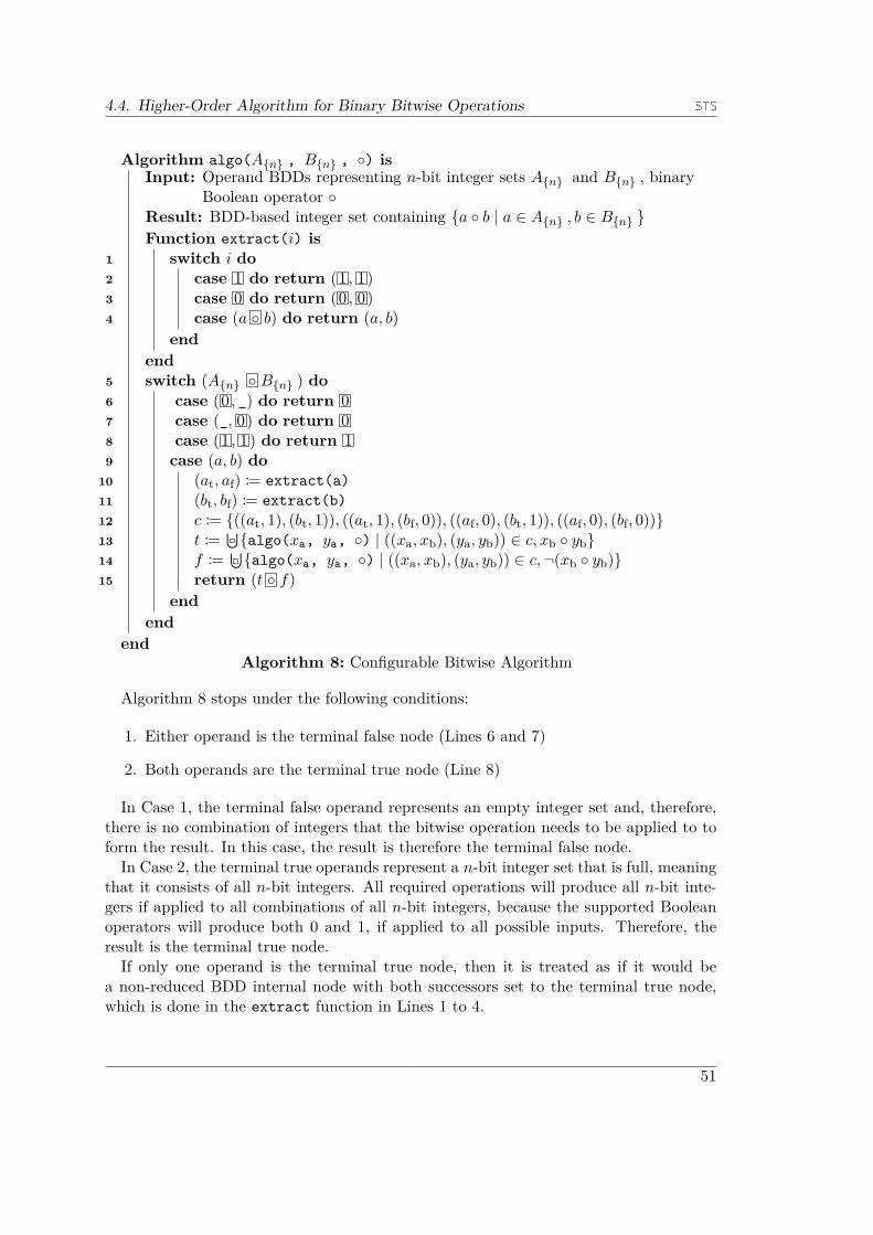
4.4. Higher-Order Algorithm for Binary Bitwise Operations

Algorithm algo(A{n} , B{n} , ◦) isInput: Operand BDDs representing n-bit integer sets A{n} and B{n} , binary

Boolean operator ◦Result: BDD-based integer set containing {a ◦ b | a ∈ A{n} , b ∈ B{n} }Function extract(i) is

1 switch i do2 case 1 do return (1 , 1)3 case 0 do return (0 , 0)4 case (a ◦ b) do return (a, b)

endend

5 switch (A{n} ◦ B{n} ) do6 case (0 , _) do return 07 case (_, 0) do return 08 case (1 , 1) do return 19 case (a, b) do

10 (at, af) := extract(a)11 (bt, bf) := extract(b)12 c := {((at, 1), (bt, 1)), ((at, 1), (bf, 0)), ((af, 0), (bt, 1)), ((af, 0), (bf, 0))}13 t := ⋃

{algo(xa, ya, ◦) | ((xa, xb), (ya, yb)) ∈ c, xb ◦ yb}14 f := ⋃

{algo(xa, ya, ◦) | ((xa, xb), (ya, yb)) ∈ c,¬(xb ◦ yb)}15 return (t ◦ f)

endend

endAlgorithm 8: Configurable Bitwise Algorithm

Algorithm 8 stops under the following conditions:

1. Either operand is the terminal false node (Lines 6 and 7)

2. Both operands are the terminal true node (Line 8)

In Case 1, the terminal false operand represents an empty integer set and, therefore,there is no combination of integers that the bitwise operation needs to be applied to toform the result. In this case, the result is therefore the terminal false node.In Case 2, the terminal true operands represent a n-bit integer set that is full, meaning

that it consists of all n-bit integers. All required operations will produce all n-bit inte-gers if applied to all combinations of all n-bit integers, because the supported Booleanoperators will produce both 0 and 1, if applied to all possible inputs. Therefore, theresult is the terminal true node.If only one operand is the terminal true node, then it is treated as if it would be

a non-reduced BDD internal node with both successors set to the terminal true node,which is done in the extract function in Lines 1 to 4.

51

4. BDDStab Library

The only missing case is when both operands are non-terminal. In this case (Lines 9to 15), each operand node can be deconstructed into a true and false successor sub-BDDusing the extract function. The successor sub-BDDs under the true edge, i.e., at andbt in this case, represent the sets of integers with the corresponding bit set, and the falsesuccessors, i.e., af, and bf, represent the sets with the bit unset. Since the algorithm mustcompute a result in Cartesian product fashion, it must consider all combinations of thesuccessors of both inputs A{n} and B{n} , hence the construction of c in Line 12. Thisc not only contains tuples of all combinations of sub-BDDs, but additionally a Booleanthat indicates whether this sub-BDD was a true or a false successor, which is equivalentto the value of the bit at the current position. These additional Booleans are used inLines 13 and 14, where the true and false successor of the result node are constructed.The construction of the true successor, in Line 13, only uses those combinations from cwhere the given Boolean operator ◦, applied to the corresponding Booleans, yields true.The algorithm is called recursively on all these combinations and the results of these callsare merged using integer set union, i.e., a disjunction at BDD level. The construction ofthe false successor in Line 14 applies the same operations on those combinations from cwhere the Boolean operator yields false.In the following, we will compute algo(A2, B2, ∧), where A2 = {0, 3} and B2 ={1, 2}. Figure 4.8 lists the corresponding BDDs of the two bit integer sets.

algo(A{2} , B{2} , ∧) =(algo(A{1} , B{1} , ∧)◦⋃{algo(A{1} , B′{1} , ∧), algo(A′{1} , B{1} , ∧), algo(A′{1} , B′{1} , ∧)})

In the first recursive step, only the combination (A{1} , B{1} ) gets selected for the truesuccessor of the result node, since only these BDDs are true successors and thereforecorrespond to sub-BDDs with an incoming true edge, and a ∧ b is only true if both aand b are; all other combinations are selected for the false successor of the result node.

algo(A{1} , B{1} , ∧) =(algo(1, 0, ∧) ◦

⋃{algo(1, 1, ∧), algo(0, 0, ∧), algo(0, 1, ∧)}) =

(0 ◦ 1)

With the above result, the algorithm has computed that 2 is included in the resultset, since (0 ◦ 1) is set under the true edge of the result node. In the following, thealgorithm computes the node for the false successor of the result node.

algo(A{1} , B′{1} , ∧) =(algo(1, 1, ∧) ◦

⋃{algo(1, 0, ∧), algo(0, 1, ∧), algo(0, 0, ∧)}) =

(1 ◦ 0)

algo(A′{1} , B{1} , ∧) =(algo(0, 0, ∧) ◦

⋃{algo(0, 1, ∧), algo(1, 0, ∧), algo(1, 1, ∧)}) =

(0 ◦ 1)

52

4.5. Arithmetic Operations

algo(A′{1} , B′{1} , ∧) =(algo(0, 1, ∧) ◦

⋃{algo(0, 0, ∧), algo(1, 1, ∧), algo(1, 0, ∧)}) =

(0 ◦ 1)

The false successor of the outer result node is the union of all of the above threeintermediate results, i.e., 1 . Hence, the result of the computation is {2, 1, 0}, just asexpected.

A{2}

A{1} A′{1}

1 0 0 1

B{2}

B{1} B′{1}

0 1 1 0

Figure 4.8.: BDDs of A{2} on the left, and B{2} on the right

Optimization

Algorithm 8 produces the desired results, but it can be improved in terms of efficiency. Ifc in Line 12 contains two tuples where the BDDs are equal and only the bit informationdiffers, the recursive call must only be applied once and its result can be copied forthe other tuple. This optimization is included in the memoization technique. Further,all of the targeted Boolean operators are commutative. Hence, c can be reduced byremoving tuples that differ in the order the BDDs appear. This optimization can also beimplemented using memoization by checking whether a call to the algorithm with flippedarguments is cached. If these optimizations are to be implemented using memoizationit must be ensured that cache entries outlive the call of the algorithm, since otherwise,it could be that cached results are dropped before becoming useful in the next recursivealgorithm call.

4.5. Arithmetic Operations

In difference to the bitwise variations of the binary Boolean operators discussed before,in arithmetic operations, an output bit at position n is not uniquely determined by theinput bits at position n. Therefore, Algorithm 8 is not directly applicable for addition.In this section, we therefore adapt Algorithm 8 to addition and subtraction, and provideapproximating algorithms for multiplication and division, as well as precise versions forspecial cases.

53

4. BDDStab Library

Addition

Algorithm 8 takes one of the common binary Boolean operators, and computes thebitwise version of the operator on integer sets. The corresponding Boolean operatorfor addition is the full adder, which we will use to design an algorithm that supportsaddition. Since overflow behavior is defined on machine code level, this algorithm mustprecisely simulate overflow.A full adder takes three Boolean inputs, and produces two boolean outputs, i.e., sum

and carry. Equation 4.4 defines the sum (s) and carry (cout) outputs depending on theinput Booleans a, b, and cin.

s(a, b, cin) = a Y b Y cincout(a, b, cin) = (a ∧ b) ∨ b(∧cin) ∨ (a ∧ cin) (4.4)

To produce an n-bit adder, the full adders are combined as described in Equation 4.5.

c{0} = 0c{i} = cout(a{i−1} , b{i−1} , c{i−1} )o{i} = s(a{i} , b{i} , c{i} )

(4.5)

From these equations, we know that to determine a bit at position i, we need not onlyknow the two input bits a{i} and b{i} , but also the carry information as computed fromposition i−1. Therefore, each recursive call must additionally produce carry information.We modify the algorithm to return two BDD-based integer sets instead of one. One setrepresents the resulting integer sets without values that are the result from overflow,and one set represents only values that result from overflow. This modification allowsthe communication of the carry information as required, since values that result fromoverflow are values that have the carry bit set. Unioning the carry and non-carry resultproduces a correct result if traditional wrap-around semantics is assumed. Since thecarry information from bit position n influences the calculation for bit position n + 1,it can be said to propagate from LSB to MSB. The formulation of an algorithm foraddition and subtraction would therefore benefit from LSB to MSB ordering in theBDD. However, our algorithm must support MSB to LSB ordering for the reasons givenin Section 4.2.Algorithm 9 is an adaptation of Algorithm 8 to support a full adder as operator. The

algorithm uses the extract function from Algorithm 8, as well as the ival2bdd function(Algorithm 4) that takes a lower and an upper bound and creates a BDD integer setcontaining elements within the bounds. In the base cases where one input BDD is 0(Lines 2 and 3), the algorithm returns 0 for the non-overflow BDD in the first elementof the returned tuple, and 0 as the overflow BDD in the second element of the tuple.The reason for returning 0 is that one of the input integer sets does not contain anyelements, therefore the Cartesian product is empty.In case both input BDDs are 1 (line 4), i.e., the represented n-bit integer set contains

all n-bit integers, then the non-overflow BDD must contain all n-bit integers as wellbecause one such integer set contains 0 and {0}+# {i | 0 ≤ i < 2n} is {i | 0 ≤ i < 2n}.

54

4.5. Arithmetic Operations

The overflow result contains all but the largest n-bit integer, since the largest overflowresult is 2n − 1 + 2n − 1 = 2n+1 − 2 and the MSB is treated as unset to simulatewrap-around.

The recursive case is in Lines 8 to 18. First, the true and false successors of theroots of the input BDDs are extracted (Lines 9 and 10). Similarly to Algorithm 8, allcombinations of the successors are built in Lines 11 to 13. In difference to Algorithm8, each recursive call generates two results, one non-overflow result and one overflowresult, which both get stored in cab together with the input bit information and carryinformation. Lines 14 to 17 compute the successor for the overflow and non-overflowresults by applying the given operator, which for addition is the full adder, and selectingand merging the corresponding BDDs.

Algorithm add(A{n} , B{n} , ◦, d = n) isInput: Operand BDDs representing n-bit integer sets A{n} and B{n} , ternary

Boolean operator ◦, depth dResult: BDD-based integer sets containing overflow and non-overflow results

1 switch (A{n} , B{n} ) do2 case (0 , _) do return (0 , 0)3 case (_, 0) do return (0 , 0)4 case (1 , 1) do5 if d = 0 then6 return (1 , 0)

else7 return (1 , ival2bdd(0, 2d − 2))

endend

8 case (a, b) do9 (at, af) := extract(a)

10 (bt, bf) := extract(b)11 ca := {(at, 1), (af, 0)}12 cb := {(bt, 1), (bf, 0)}13 cab := ⋃

{{(z, ya, yb, 0), (zc, ya, yb, 1)} | (xa, ya) ∈ ca, (xb, yb) ∈ cb, (z, zc) =add(xa, xb, ◦, d = d− 1)}

14 t := ⋃{z | (z, ya, yb, c) ∈ cab, (r, cr) = ◦(ya, yb, c), r,¬cr}

15 tc := ⋃{z | (z, ya, yb, c) ∈ cab, (r, cr) = ◦(ya, yb, c), r, cr}

16 f := ⋃{z | (z, ya, yb, c) ∈ cab, (r, cr) = ◦(ya, yb, c),¬r,¬cr}

17 fc := ⋃{z | (z, ya, yb, c) ∈ cab, (r, cr) = ◦(ya, yb, c),¬r, cr}

18 return ((t ◦ f), (tc ◦ fc))end

endend

Algorithm 9: Algorithm Supporting Addition and Subtraction

55

4. BDDStab Library

As an example, we use Algorithm 9 to compute A{1} +# B{1} , where A{1} = {1}and B{1} = {0, 1}. In 1-bit unsigned arithmetic with wrap-around, we would expectthe result of the above computation to be {0, 1}, since 1 + 0 = 1 and 1 + 1 = 2, whichis 0 in one bit arithmetic with overflow. We therefore expect the algorithm to return({1}, {0}), since {1} is the non-overflow part of the result and {0} is the overflow partof the result. Unioning of the overflow and non-overflow results will obtain the desiredresult with overflow simulation. The BDDs of A{1} and B{1} are shown in Figure 4.9.Note that B{1} is the terminal true node, since it represents the set of all 1-bit integers.

A{1}

1 0

1

Figure 4.9.: BDDs of A{1} on the left, and B{1} on the right

Algorithm 9, applied to A{1} and B{1} , proceeds as follows:

add(A{1} , B{1} , fAdder(), d = 1) =cab := {(z11, 1, 1, 0), (z11c, 1, 1, 1), (z10, 1, 0, 0), (z10c, 1, 0, 1)

, (z01, 0, 1, 0), (z01c, 0, 1, 1), (z00, 0, 0, 0), (z00c, 0, 0, 1)| (z11, z11c) = add(1, 1, fAdder(), d = 0) = (1 , 0), (z10, z10c) = add(1, 1, fAdder(), d = 0) = (1 , 0), (z01, z01c) = add(0, 1, fAdder(), d = 0) = (0 , 0), (z00, z00c) = add(0, 1, fAdder(), d = 0)} = (0 , 0)

= {(1 , 1, 1, 0), (0 , 1, 1, 1), (1 , 1, 0, 0), (0 , 1, 0, 1), (0 , 0, 1, 0), (0 , 0, 1, 1), (0 , 0, 0, 0), (0 , 0, 0, 1)}

t := ⋃{1 , 0 , 0} = 1

tc := ⋃{0} = 0

f := ⋃{0} = 0

fc := ⋃{1 , 0 , 0} = 1

return((1 ◦ 0), (0 ◦ 1))

When applied to A{1} , B{1} , and depth 1 corresponding to the bitwidth of the inputinteger sets, the algorithm executes the recursive switch case (Lines 8 to 18). Conse-quently, the successors of the input BDDs are extracted and all required combinationsare built with the corresponding results of the recursive addition calls in cab, while retain-ing the information from which edges the combination was built. The recursive additioncalls with 0 as one of the arguments will return (0 , 0) according to the switch cases inLines 2 and 3. The recursive addition calls with 1 for both arguments will return (1 , 0)according to the switch case in Lines 4 to 7 since d is 0. The non-overflow true edgeBDD (t) gets constructed from those tuples in cab that have one set bit in the last threetuple elements, because only then will the full adder return 1 for the sum and 0 for the

56

4.5. Arithmetic Operations

carry. Likewise, only the tuple with all bits set is selected for tc, since only then will thefull adder return 1 for the sum and carry. The non-overflow false edge BDD (f) is builtfrom the tuple with all bits set to 0, all other tuples are selected for the remaining falseedge BDD of the overflow result. Hence, the result is ((1 ◦ 0), (0 ◦ 1)), which is theexpected ({1}, {0}) in integer set-interpretation.

Optimizations

Algorithm 9 can be optimized, but one must be careful not to change the function ofthe algorithm. For example, it may be tempting to replace the case where both inputBDDs are equal, which can, of course, be checked in O(1), by multiplication of two orshift left of one. However, this would be incorrect, since the algorithm must computeits result in the previously outlined Cartesian product fashion. In other words, equalityof two variation domains does not imply that the corresponding variables, for which theVDs were computed, are equal. Therefore, such optimization can only be done outsideof the algorithm, if equality can be proven.More optimization potential can be found in the unification of the BDDs for t and

fc. The full adder will always select three BDDs for t and fc, since there are threeinputs with one set bit, and also three inputs with two set bits. Therefore, insteadof defining unification of a set of BDD-based integer sets using repeated applicationof binary unification, which requires two BDD traversals, we specialize union of threeBDD-based integers sets in Algorithm 10.

Algorithm merge3(A, B, C) isInput: Three BDD-based integer setsResult: Union of given BDD-based integer sets

1 switch (A,B,C) do2 case (1 , _, _) do return 13 case (_, 1 , _) do return 14 case (_, _, 1) do return 15 case (0 , _, _) do return B ∪ C6 case (_, 0 , _) do return A ∪ C7 case (_, _, 0) do return A ∪B8 case ((Aa ◦ Ab), (Ba ◦ Bb), (Ca ◦ Cb)) do9 t := merge3(Aa, Ba, Ca)

10 f := merge3(Ab, Bb, Cb)11 return (t ◦ f)

endend

endAlgorithm 10: Algorithm for Unification of Three BDD-based Integer Sets

Another substantial optimization for Algorithm 9 is the addition of base cases specificto addition. Currently, the algorithm only stops its recursion if at least one operand

57

4. BDDStab Library

is 0 , or both operands are 1 . However, it is possible to extend the algorithm to alsostop its recursion when at least one operand is 1 . Whenever one of the arguments is 1 ,this 1 represents an interval of all n-bit integers (A = [0 .. 2n − 1]), whereas the otherrepresents a set of n-bit integers B. Since A is the set of all n bit integers, we concludeB ⊆ A. The distance between any two elements in B is less than the width of A,and hence all intervals that result from adding a number from B to each element in Awill overlap. Therefore, the non-overflow result will be an interval, starting at the leastelement in B (min(B) = min(B) + min(A)) to the maximum n-bit integer (max(A)).The overflow result will be an interval from 0 to the greatest element in B minus one,since max(B) + max(A) = max(B) + 2n− 1 = max(B)− 1(mod 2n). Algorithm 11 lists theoptimized addition algorithm.

Algorithm add(A{n} , B{n} , d) isInput: Operand BDDs representing n-bit integer sets A{n} and B{n}Result: BDD-based integer sets containing overflow and non-overflow results

1 switch (A{n} , B{n} ) do2 case (0 , _) do return (0 , 0)3 case (_, 0) do return (0 , 0)4 case (1 , _) do return

(ival2bdd(min(B{n} ), max(A{n} )), ival2bdd(0, max(B{n} )− 1))5 case (_, 1) do return add(B{n} , A{n} , d)6 case ((At ◦ Af), (Bt ◦ Bf)) do7 (x11, xc11) := add(At, Bt, d− 1)8 (x10, xc10) := add(At, Bf, d− 1)9 (x01, xc01) := add(Af, Bt, d− 1)

10 (x00, xc00) := add(Af, Bf, d− 1)11 t := merge3(x10, x01, xc00)12 tc := xc1113 f := x0014 fc := merge3(x11, xc10, xc01)15 return ((t ◦ f), (tc ◦ fc))

endend

endAlgorithm 11: Optimized Algorithm for Addition

Correctness of Addition

In this paragraph, we will discuss the correctness of Algorithm 11. We will assumecorrectness of the ival2bdd algorithm that constructs BDD representation of intervals,as well as correctness of merge3, which unifies three BDD-based sets. In the proof, weuse the induction scheme as described in Section 4.1.2.First, let us define the correctness property for addition (P in the induction scheme).

58

4.5. Arithmetic Operations

As previously discussed, abstract interpretation demands that if a correctness relationexists between the concrete and abstract values for the input of an operation, thenthe outputs of the corresponding transfer function must also be correct with respectto the output of the operation. For the addition transfer function on non-relational,unsigned n-bit integer sets A{n} and B{n} this requirement applies as well. However,our addition algorithm returns a tuple of two BDDs, one for the non-overflow and onefor the overflow result. Therefore, we first define the functions h and g that convertbetween a tuple of non-overflow (Rcarry

{n} ) and overflow result (Rcarry{n} ) and addition via

the Cartesian product:

h(R{n+1} ) = ({r | r ∈ R{n+1} , r < 2n}, {r − 2n | r ∈ R{n+1} , r ≥ 2n})g((Rcarry

{n} , Rcarry{n} )) = R

carry{n} ∪ {r + 2n | r ∈ Rcarry

{n} }

Next, we prove that h and g together form a bijection by showing h ◦ g = id andg ◦ h = id.

Assuming R = L ∪B with ∀l ∈ L : 0 ≤ l < 2n and ∀b ∈ B : 2n ≤ b < 2n+1 we get:h(R) = h(L ∪B) = (L, {r − 2n | r ∈ B}) andg((L, {r − 2n | r ∈ B}))

= L ∪ {r′ + 2n | r′ ∈ {r − 2n | r ∈ B}}= L ∪ {r′ | r′ ∈ B}= L ∪B= R

Hence, g ◦ h = id.

Assuming L and B with ∀l ∈ L : 0 ≤ l < 2n and ∀b ∈ B : 0 ≤ b < 2n we get:g((L,B)) = g(({l | l ∈ L, 0 ≤ l < 2n}, {b | b ∈ B, 0 ≤ b < 2n}))

= {l | l ∈ L, 0 ≤ l < 2n} ∪ {r + 2n | r ∈ {b | b ∈ B, 0 ≤ b < 2n}}= {l | l ∈ L, 0 ≤ l < 2n} ∪ {b | b ∈ {r + 2n | r ∈ B, 0 ≤ r < 2n}, 2n ≤ b < 2n+1}

h({l | l ∈ L, 0 ≤ l < 2n} ∪ {b | b ∈ {r + 2n | r ∈ B, 0 ≤ r < 2n}, 2n ≤ b < 2n+1})= (L, {r − 2n | r ∈ {b+ 2n | b ∈ B}})= (L, {r − 2n + 2n | r ∈ B})= (L,B)

Hence, h ◦ g = id.�

We further observe the following equalities:(A{n} ◦ B{n} ) = {a+ 2n | a ∈ A{n} } ∪B{n} = g((B{n} , A{n} ))0{n} = ∅1{n} = {e | 0 ≤ e < 2n}merge3(A{n} , B{n} , C{n} ) = A{n} ∪B{n} ∪ C{n}

The correctness property P for addition is defined as follows:

59

4. BDDStab Library

P (X{n} , Y{n} ) ⇐⇒ h({x+ y | x ∈ X{n} , y ∈ Y{n} }) = add(X{n} , Y{n} , n)

In other words, if addition via the Cartesian product is executed and the result, usingh, is partitioned into values that fit into the original n-bit range and those that do not,then this partition must be returned by the addition algorithm. In the following, weprove P for arbitrary tuples of BDDs using the induction scheme described in Section4.1.2. Hence, we have to prove the following:

Base Cases:

∀A{n} : P (A{n} , 0) (4.6)

∀B{n} : P (0 , B{n} ) (4.7)

∀A{n} : P (A{n} , 1) (4.8)

∀B{n} : P (1 , B{n} ) (4.9)

Inductive Case:

P (A{n} , C{n} ) ∧ P (A{n} , D{n} ) ∧ P (B{n} , C{n} ) ∧ P (B{n} , D{n} )=⇒ P ((A{n} ◦ B{n} ), (C{n} ◦ D{n} )) (4.10)

Proofs

Proof of 4.6:h({a+ b | a ∈ A{n} , b ∈ 0}) = add(A{n} , 0 , n)=⇒ ∅ = add(A{n} 0 , n)=⇒ ∅ = 0{n}=⇒ ∅ = ∅

Proof 4.7: Analog to ∀A{n} : P (A{n} , 0).Proof of 4.8:

60

4.5. Arithmetic Operations

h({a+ b | a ∈ A{n} , b ∈ 1}) = add(A{n} , 1 , n)⇐⇒ h({a+ b | a ∈ A{n} , b ∈ 1{n} }) = add(A{n} , 1 , n)⇐⇒ h({a+ b | a ∈ A{n} , b ∈ {e | 0 ≤ e < 2n}}) = add(A{n} , 1 , n)Hence, A{n} ∈ {e | 0 ≤ e < 2n}, and since {e | 0 ≤ e < 2n} is convex,{a+ b | a ∈ A{n} , b ∈ {e | 0 ≤ e < 2n}} is convex as well.Setting X{n+1} = {a+ b | a ∈ A{n} , b ∈ {e | 0 ≤ e < 2n}} we get:h({e | min(X{n+1} ) ≤ e ≤ max(X{n+1} )}) = add(A{n} , 1 , n)⇐⇒ h({e | min(A{n} ) ≤ e ≤ max(A{n} ) + 2n − 1}) = add(A{n} , 1 , n)⇐⇒ {e | min(A{n} ) ≤ e ≤ max(A{n} ) + 2n − 1} = g(add(A{n} , 1 , n))

Assuming correctness of ival2bdd, we have:g(add(A{n} , 1 , n))= g((ival2bdd(min(A{n} ), max(1)), ival2bdd(0, max(A{n} )− 1)))= g((ival2bdd(min(A{n} ), 2n − 1), ival2bdd(0, max(A{n} )− 1)))= g(({e | min(A{n} ) ≤ e ≤ 2n − 1}, {e | 0 ≤ e ≤ max(A{n} )− 1}))= {e | min(A{n} ) ≤ e ≤ 2n − 1} ∪ {e+ 2n | 0 ≤ e ≤ max(A{n} )− 1}= {e | min(A{n} ) ≤ e ≤ 2n − 1} ∪ {e | 2n ≤ e ≤ max(A{n} ) + 2n − 1}= {e | min(A{n} ) ≤ e ≤ max(A{n} ) + 2n − 1}

Proof of 4.9: Analog to ∀A{n} : P (A{n} , 1).

Inductive Case

Proof of 4.10:

( P (A{n} , C{n} ) ∧ P (A{n} , D{n} ) ∧ P (B{n} , C{n} ) ∧ P (B{n} , D{n} )=⇒ P ((A{n} ◦ B{n} ), (C{n} ◦ D{n} ))) ⇐⇒ ( h({a+ c | a ∈ A{n} , c ∈ C{n} }) = add(A{n} , C{n} , n)

∧h({a+ d | a ∈ A{n} , d ∈ D{n} }) = add(A{n} , D{n} , n)∧h({b+ c | b ∈ B{n} , c ∈ C{n} }) = add(B{n} , C{n} , n)∧h({b+ d | b ∈ B{n} , d ∈ D{n} }) = add(B{n} , D{n} , n)

=⇒ h({s+ u | s ∈ (A{n} ◦ B{n} ), u ∈ (C{n} ◦ D{n} )})= add((A{n} ◦ B{n} ), (C{n} ◦ D{n} ), n+ 1)

)(4.11)

First, we operate on the right-hand side of the consequent in Equation 4.11 and expandthe recursive calls to add using the induction hypothesis:

61

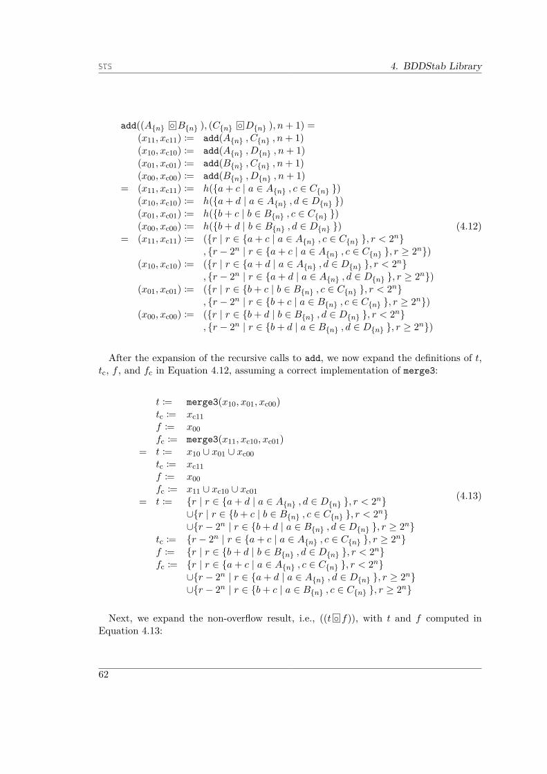
4. BDDStab Library

add((A{n} ◦ B{n} ), (C{n} ◦ D{n} ), n+ 1) =(x11, xc11) := add(A{n} , C{n} , n+ 1)(x10, xc10) := add(A{n} , D{n} , n+ 1)(x01, xc01) := add(B{n} , C{n} , n+ 1)(x00, xc00) := add(B{n} , D{n} , n+ 1)

= (x11, xc11) := h({a+ c | a ∈ A{n} , c ∈ C{n} })(x10, xc10) := h({a+ d | a ∈ A{n} , d ∈ D{n} })(x01, xc01) := h({b+ c | b ∈ B{n} , c ∈ C{n} })(x00, xc00) := h({b+ d | b ∈ B{n} , d ∈ D{n} })

= (x11, xc11) := ({r | r ∈ {a+ c | a ∈ A{n} , c ∈ C{n} }, r < 2n}, {r − 2n | r ∈ {a+ c | a ∈ A{n} , c ∈ C{n} }, r ≥ 2n})

(x10, xc10) := ({r | r ∈ {a+ d | a ∈ A{n} , d ∈ D{n} }, r < 2n}, {r − 2n | r ∈ {a+ d | a ∈ A{n} , d ∈ D{n} }, r ≥ 2n})

(x01, xc01) := ({r | r ∈ {b+ c | b ∈ B{n} , c ∈ C{n} }, r < 2n}, {r − 2n | r ∈ {b+ c | a ∈ B{n} , c ∈ C{n} }, r ≥ 2n})

(x00, xc00) := ({r | r ∈ {b+ d | b ∈ B{n} , d ∈ D{n} }, r < 2n}, {r − 2n | r ∈ {b+ d | a ∈ B{n} , d ∈ D{n} }, r ≥ 2n})

(4.12)

After the expansion of the recursive calls to add, we now expand the definitions of t,tc, f , and fc in Equation 4.12, assuming a correct implementation of merge3:

t := merge3(x10, x01, xc00)tc := xc11f := x00fc := merge3(x11, xc10, xc01)

= t := x10 ∪ x01 ∪ xc00tc := xc11f := x00fc := x11 ∪ xc10 ∪ xc01

= t := {r | r ∈ {a+ d | a ∈ A{n} , d ∈ D{n} }, r < 2n}∪{r | r ∈ {b+ c | b ∈ B{n} , c ∈ C{n} }, r < 2n}∪{r − 2n | r ∈ {b+ d | a ∈ B{n} , d ∈ D{n} }, r ≥ 2n}

tc := {r − 2n | r ∈ {a+ c | a ∈ A{n} , c ∈ C{n} }, r ≥ 2n}f := {r | r ∈ {b+ d | b ∈ B{n} , d ∈ D{n} }, r < 2n}fc := {r | r ∈ {a+ c | a ∈ A{n} , c ∈ C{n} }, r < 2n}

∪{r − 2n | r ∈ {a+ d | a ∈ A{n} , d ∈ D{n} }, r ≥ 2n}∪{r − 2n | r ∈ {b+ c | a ∈ B{n} , c ∈ C{n} }, r ≥ 2n}

(4.13)

Next, we expand the non-overflow result, i.e., ((t ◦ f)), with t and f computed inEquation 4.13:

62

4.5. Arithmetic Operations

(t ◦ f) = g(f, t) ={r | r ∈ {b+ d | b ∈ B{n} , d ∈ D{n} }, r < 2n}∪{r′ + 2n | r′ ∈{r | r ∈ {a+ d | a ∈ A{n} , d ∈ D{n} }, r < 2n}∪{r | r ∈ {b+ c | b ∈ B{n} , c ∈ C{n} }, r < 2n}∪{r − 2n | r ∈ {b+ d | a ∈ B{n} , d ∈ D{n} }, r ≥ 2n}}

= {r | r ∈ {b+ d | b ∈ B{n} , d ∈ D{n} }, r < 2n}∪{r + 2n | r ∈ {a+ d | a ∈ A{n} , d ∈ D{n} }, r < 2n}∪{r + 2n | r ∈ {b+ c | b ∈ B{n} , c ∈ C{n} }, r < 2n}∪{r | r ∈ {b+ d | a ∈ B{n} , d ∈ D{n} }, r ≥ 2n}

(4.14)

Now, we expand the overflow result, i.e., ((tc ◦ fc)), with tc and fc given by Equation4.13:

(tc ◦ fc) = g(fc, tc) ={r | r ∈ {a+ c | a ∈ A{n} , c ∈ C{n} }, r < 2n}∪{r − 2n | r ∈ {a+ d | a ∈ A{n} , d ∈ D{n} }, r ≥ 2n}∪{r − 2n | r ∈ {b+ c | a ∈ B{n} , c ∈ C{n} }, r ≥ 2n}∪{r − 2n + 2n | r ∈ {a+ c | a ∈ A{n} , c ∈ C{n} }, r ≥ 2n}

= {r | r ∈ {a+ c | a ∈ A{n} , c ∈ C{n} }, r < 2n}∪{r − 2n | r ∈ {a+ d | a ∈ A{n} , d ∈ D{n} }, r ≥ 2n}∪{r − 2n | r ∈ {b+ c | a ∈ B{n} , c ∈ C{n} }, r ≥ 2n}∪{r | r ∈ {a+ c | a ∈ A{n} , c ∈ C{n} }, r ≥ 2n}

(4.15)

In the following, we use the fact that g ◦ h = id and insert the results, obtained usingEquation 4.14 and 4.15, into the consequent of Equation 4.11:

h({s+ u | s ∈ (A{n} ◦ B{n} ), u ∈ (C{n} ◦ D{n} )}) =add((A{n} ◦ B{n} ), (C{n} ◦ D{n} ), n+ 1)

⇐⇒ {s+ u | s ∈ (A{n} ◦ B{n} ), u ∈ (C{n} ◦ D{n} )} =g(add((A{n} ◦ B{n} ), (C{n} ◦ D{n} ), n+ 1))

⇐⇒ {s+ u | s ∈ (A{n} ◦ B{n} ), u ∈ (C{n} ◦ D{n} )} =g((g(f, t), g(fc, tc)))

(4.16)

Next, we expand and rewrite the right-hand side of Equation 4.16. Note that the colorsdenote elements of a partition, i.e., subsets X ∈ Z and Y ∈ Z such that X ∩ Y = ∅ andX ∪ Y = Z. Furthermore ∃p : (∀x ∈ X : p(x)∧ ∀y ∈ Y : ¬p(y)), whenever we may unifythe colored sets and drop the predicate:

63

4. BDDStab Library

g(g(f, t), g(fc, tc)) ={r | r ∈ {b+ d | b ∈ B{n} , d ∈ D{n} }, r < 2n}∪{r + 2n | r ∈ {a+ d | a ∈ A{n} , d ∈ D{n} }, r < 2n}∪{r + 2n | r ∈ {b+ c | b ∈ B{n} , c ∈ C{n} }, r < 2n}∪{r | r ∈ {b+ d | a ∈ B{n} , d ∈ D{n} }, r ≥ 2n}∪{r′ + 2n+1 | r′ ∈{r | r ∈ {a+ c | a ∈ A{n} , c ∈ C{n} }, r < 2n}∪{r − 2n | r ∈ {a+ d | a ∈ A{n} , d ∈ D{n} }, r ≥ 2n}∪{r − 2n | r ∈ {b+ c | a ∈ B{n} , c ∈ C{n} }, r ≥ 2n}∪{r | r ∈ {a+ c | a ∈ A{n} , c ∈ C{n} }, r ≥ 2n}}

= {r | r ∈ {b+ d | b ∈ B{n} , d ∈ D{n} }, r < 2n}∪{r + 2n | r ∈ {a+ d | a ∈ A{n} , d ∈ D{n} }, r < 2n}∪{r + 2n | r ∈ {b+ c | b ∈ B{n} , c ∈ C{n} }, r < 2n}∪{r | r ∈ {b+ d | a ∈ B{n} , d ∈ D{n} }, r ≥ 2n}∪{r + 2n+1 | r ∈ {a+ c | a ∈ A{n} , c ∈ C{n} }, r < 2n}∪{r + 2n | r ∈ {a+ d | a ∈ A{n} , d ∈ D{n} }, r ≥ 2n}∪{r + 2n | r ∈ {b+ c | a ∈ B{n} , c ∈ C{n} }, r ≥ 2n}∪{r + 2n+1 | r ∈ {a+ c | a ∈ A{n} , c ∈ C{n} }, r ≥ 2n}

= {r + 2n+1 | r ∈ {a+ c | a ∈ A{n} , c ∈ C{n} }, r < 2n}∪{r + 2n+1 | r ∈ {a+ c | a ∈ A{n} , c ∈ C{n} }, r ≥ 2n}∪{r + 2n | r ∈ {a+ d | a ∈ A{n} , d ∈ D{n} }, r < 2n}∪{r + 2n | r ∈ {a+ d | a ∈ A{n} , d ∈ D{n} }, r ≥ 2n}∪{r + 2n | r ∈ {b+ c | b ∈ B{n} , c ∈ C{n} }, r < 2n}∪{r + 2n | r ∈ {b+ c | a ∈ B{n} , c ∈ C{n} }, r ≥ 2n}∪{r | r ∈ {b+ d | b ∈ B{n} , d ∈ D{n} }, r < 2n}∪{r | r ∈ {b+ d | a ∈ B{n} , d ∈ D{n} }, r ≥ 2n}

= {r + 2n+1 | r ∈ {a+ c | a ∈ A{n} , c ∈ C{n} }}∪{r + 2n | r ∈ {a+ d | a ∈ A{n} , d ∈ D{n} }}∪{r + 2n | r ∈ {b+ c | b ∈ B{n} , c ∈ C{n} }}∪{r | r ∈ {b+ d | b ∈ B{n} , d ∈ D{n} }}

= {(a+ c+ 2n+1)n + 2 | a ∈ A{n} , c ∈ C{n} }∪{(a+ d+ 2n)n + 2 | a ∈ A{n} , d ∈ D{n} }∪{(b+ c+ 2n)n + 2 | b ∈ B{n} , c ∈ C{n} }∪{b+ d | b ∈ B{n} , d ∈ D{n} }

(4.17)

Lastly, we rewrite the left-hand side of Equation 4.16 to show that it is equal to thatof Equation 4.17.

64

4.5. Arithmetic Operations

{s+ u | s ∈ (A{n} ◦ B{n} ), u ∈ (C{n} ◦ D{n} )}= {s+ u | s ∈ g(B{n} , A{n} ), u ∈ g(D{n} , C{n} )= {s+ u | s ∈ {r + 2n | r ∈ A{n} } ∪B{n} , u ∈ {r + 2n | r ∈ C{n} } ∪D{n} }= {s+ u | s ∈ {r + 2n | r ∈ A{n} }, u ∈ {r + 2n | r ∈ C{n} }}∪{s+ u | s ∈ {r + 2n | r ∈ A{n} }, u ∈ D{n} }∪{s+ u | s ∈ B{n} , u ∈ {r + 2n | r ∈ C{n} }}∪{s+ u | s ∈ B{n} , u ∈ D{n} }= {s+ u+ 2n+1 | s ∈ A{n} , u ∈ C{n} }∪{s+ u+ 2n | s ∈ A{n} , u ∈ D{n} }∪{s+ u+ 2n | s ∈ B{n} , u ∈ C{n} }∪{s+ u | s ∈ B{n} , u ∈ D{n} }

(4.18)Hence, the two left- and right-hand sides of the consequent in Equation 4.11 are equal,

which concludes our proof. �

Multiplication

In the algorithms for binary bitwise operations and addition, we used the fact thateach output bit at position n is determined by input bits at position n plus a carrybit computed at position n − 1. The fact that at most one bit of information must becommunicated from position n− 1 to n resulted in our algorithm returning two BDDs,one for a set carry bit and one for an unset carry bit, which in turn means that weonly have to do 21 recursive calls in the worst case. With multiplication, however,the number of additional information that must be transported from one recursive callto another is not constant, but instead grows with the length of the input bitvectors.Hence, the number of required recursive calls in the worst case grows with the length ofthe bitvectors, which is not acceptable.

An alternative idea is to express multiplication using shift left and addition, as is donein the Egyptian method [72]. The assumption of this method is that addition and mul-tiplication by 0, 1, and 2 (shift left) are cheaper operations than general multiplication.These assumptions are true for BDD-based integer sets, as multiplication by 0 and 1 aretrivial and we support addition as well as shift left (see Section 4.6).Figure 4.10 shows how two 3-bit integers are multiplied using the Egyptian method.

First, the integer b is shifted by the bit position of integer a, and then multiplied by thecorresponding bit in a, i.e., if the bit of a at position n is set, then b << n is added tothe result, otherwise it is not. This multiplication is an example of more than one carrybit influencing one output bit. Both the carries produced from positions 2 (value 22) and3 influence the value of the output at position 4, since at position 2, there are up to 4bits that are added, giving a maximum result of 4, which is 100 in binary representation.Therefore, not only the next bit position is influenced, but also the one beyond that.

65

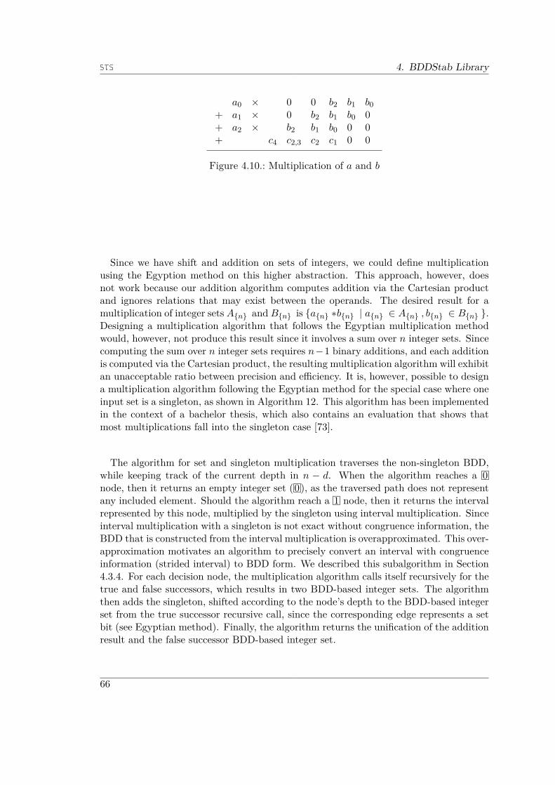
4. BDDStab Library

a0 × 0 0 b2 b1 b0+ a1 × 0 b2 b1 b0 0+ a2 × b2 b1 b0 0 0+ c4 c2,3 c2 c1 0 0

Figure 4.10.: Multiplication of a and b

Since we have shift and addition on sets of integers, we could define multiplicationusing the Egyption method on this higher abstraction. This approach, however, doesnot work because our addition algorithm computes addition via the Cartesian productand ignores relations that may exist between the operands. The desired result for amultiplication of integer sets A{n} and B{n} is {a{n} ∗b{n} | a{n} ∈ A{n} , b{n} ∈ B{n} }.Designing a multiplication algorithm that follows the Egyptian multiplication methodwould, however, not produce this result since it involves a sum over n integer sets. Sincecomputing the sum over n integer sets requires n−1 binary additions, and each additionis computed via the Cartesian product, the resulting multiplication algorithm will exhibitan unacceptable ratio between precision and efficiency. It is, however, possible to designa multiplication algorithm following the Egyptian method for the special case where oneinput set is a singleton, as shown in Algorithm 12. This algorithm has been implementedin the context of a bachelor thesis, which also contains an evaluation that shows thatmost multiplications fall into the singleton case [73].

The algorithm for set and singleton multiplication traverses the non-singleton BDD,while keeping track of the current depth in n − d. When the algorithm reaches a 0node, then it returns an empty integer set (0), as the traversed path does not representany included element. Should the algorithm reach a 1 node, then it returns the intervalrepresented by this node, multiplied by the singleton using interval multiplication. Sinceinterval multiplication with a singleton is not exact without congruence information, theBDD that is constructed from the interval multiplication is overapproximated. This over-approximation motivates an algorithm to precisely convert an interval with congruenceinformation (strided interval) to BDD form. We described this subalgorithm in Section4.3.4. For each decision node, the multiplication algorithm calls itself recursively for thetrue and false successors, which results in two BDD-based integer sets. The algorithmthen adds the singleton, shifted according to the node’s depth to the BDD-based integerset from the true successor recursive call, since the corresponding edge represents a setbit (see Egyptian method). Finally, the algorithm returns the unification of the additionresult and the false successor BDD-based integer set.

66

4.5. Arithmetic Operations

Algorithm mulSingl(A{n} , b{n} , d = n) isInput: BDD representing an n-bit integer set A{n} , an n-bit singleton b{n} ,

depth dResult: BDD-based 2n-bit integer set containing multiplication result

1 switch A{n} do2 case 1 do3 [l .. h] := [0 .. 2d − 1] ∗#[] b{n}4 return ival2bdd(l, h, 2n)

end5 case 0 do return 06 case (s ◦ u) do

7l := add(mulSingl(s, b{n} , d = d− 1),

fromNumber(b{n} << n− d, 0, 0, 1, d = 2n), 2n)8 r := mulSingl(u, b{n} , d = d− 1)9 return ite(l, 1, r)

endend

endAlgorithm 12: Multiplication with Singleton

For the cases where neither input set is a singleton, we use an approximative algorithmthat converts the input BDD-based integer sets to sets of intervals, performs intervalmultiplication in a Cartesian fashion, and converts the resulting set of intervals back toa BDD-based integer set.

Division

Algorithm 13 uses the transfer function for division of the interval abstract domain (/#[])in combination with the approximative conversion from BDD-based integer sets to setsof intervals. The algorithm’s precision can be adjusted using the parameter i, whichconfigures the precision of the conversion to interval sets.

Algorithm div(A{n} , B{n} , i) isInput: BDDs A{n} and B{n} , representing n-bit integer sets, precision

parameter i < nResult: BDD-based 2n-bit integer set containing division result

1return

⋃{ival2bdd(A/#[]B) | A ∈ bdd2ival(A{n} , i = i)

, B ∈ bdd2ival(B{n} , i = i)}end

Algorithm 13: Division via Interval Transfer Function

67

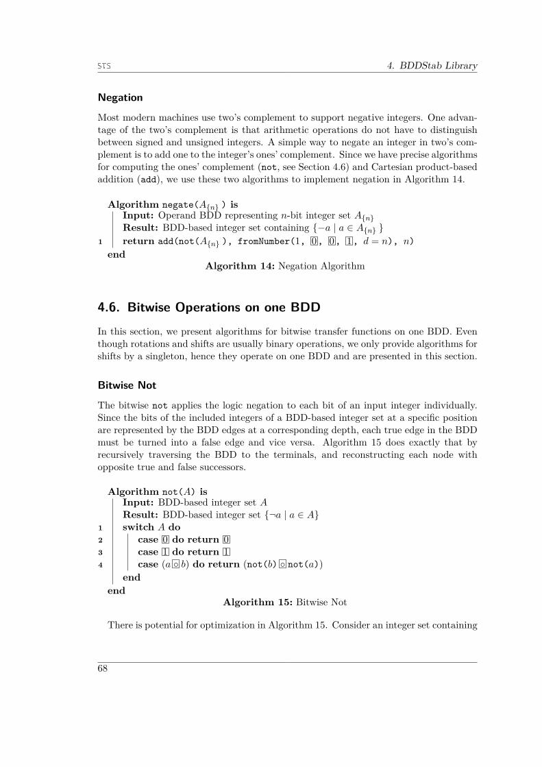
4. BDDStab Library

Negation

Most modern machines use two’s complement to support negative integers. One advan-tage of the two’s complement is that arithmetic operations do not have to distinguishbetween signed and unsigned integers. A simple way to negate an integer in two’s com-plement is to add one to the integer’s ones’ complement. Since we have precise algorithmsfor computing the ones’ complement (not, see Section 4.6) and Cartesian product-basedaddition (add), we use these two algorithms to implement negation in Algorithm 14.

Algorithm negate(A{n} ) isInput: Operand BDD representing n-bit integer set A{n}Result: BDD-based integer set containing {−a | a ∈ A{n} }

1 return add(not(A{n} ), fromNumber(1, 0, 0, 1, d = n), n)end

Algorithm 14: Negation Algorithm

4.6. Bitwise Operations on one BDD

In this section, we present algorithms for bitwise transfer functions on one BDD. Eventhough rotations and shifts are usually binary operations, we only provide algorithms forshifts by a singleton, hence they operate on one BDD and are presented in this section.

Bitwise Not

The bitwise not applies the logic negation to each bit of an input integer individually.Since the bits of the included integers of a BDD-based integer set at a specific positionare represented by the BDD edges at a corresponding depth, each true edge in the BDDmust be turned into a false edge and vice versa. Algorithm 15 does exactly that byrecursively traversing the BDD to the terminals, and reconstructing each node withopposite true and false successors.

Algorithm not(A) isInput: BDD-based integer set AResult: BDD-based integer set {¬a | a ∈ A}

1 switch A do2 case 0 do return 03 case 1 do return 14 case (a ◦ b) do return (not(b) ◦ not(a))

endend

Algorithm 15: Bitwise Not

There is potential for optimization in Algorithm 15. Consider an integer set containing

68

4.6. Bitwise Operations on one BDD

all even integers of a fixed bitwidth. Assuming n-bit integers, our BDD representationof this set consists of n decision nodes. Each of these decision nodes has its true andfalse successors set to the same sub-BDD. Hence, Algorithm 15 executes two recursivecalls per decision node, yielding exponential runtime even though n recursive calls aresufficient. Introducing a case that checks for equivalence of the two input BDDs, anduses only one recursive call in case of equivalence, alleviates this inefficiency.

Sized, Drop, and Fill

In this section, we first present helper algorithms that we will use later in this sectionto define various shift and rotation algorithms.

The sized algorithm (Algorithm 16) takes a BDD A, a target height d, and anotherBDD T , and cuts A to a depth d, and places T at all cutting points. This algorithm isused to limit the height of A.

Algorithm sized(A, d, T) isInput: BDD A, target height d, path end BDD TResult: BDD with maximum height d+ depth(T )

1 if d = 0 then return T2 switch A do3 case 0 do 04 case 1 do 15 case (S ◦ U) do6 return (sized(S, d− 1, T) ◦ sized(U, d− 1, T))

endend

endAlgorithm 16: Sized

Algorithm 17 removes the first n decision nodes from a given BDD A, by computingthe disjunction of all sub-BDDs at depth n.

69

4. BDDStab Library

Algorithm drop(A{n} , d) isInput: BDD A{n} , bits to drop dResult: BDD with maximum height n− d, with the first d bits dropped

1 if n = 0 then return {A}2 switch A do3 case 0 do return 04 case 1 do return 15 case (S ◦ U) do6 ite(drop(S, n - 1), 1, drop(U, n - 1))

endend

endAlgorithm 17: Drop

The fill algorithm (Algorithm 18) takes a depth d and a BDD T , and places T at theend of a chain of decision nodes where both outgoing edges point to the next element inthe chain. This operation is therefore equivalent to shifting the ordering of the variablesin the BDD, because the root node of T becomes a decision node at depth d in theresulting BDD.

Algorithm fill(d, T) isInput: Number of bits to ignore d, BDD to end paths TResult: BDD with maximum height d+ depth(T ), ignoring the first d bits

1 if d = 0 then2 return T

else3 temp := fill(d− 1, T)4 return (temp ◦ temp)

endend

Algorithm 18: Fill

The bitExtract algorithm (Algorithm 19) combines sized and drop to perform slic-ing at the bit level. It takes an integer set A{n} , a high bit position h, and a low bitposition l, and returns an h− l bit integer set that contains only the bits between h andl of all integers in A{n} . The algorithm can be used to model shadow registers, used inx86 assembly.

Algorithm bitExtract(A{n} , h, l) isInput: n-bit integer set A{n} , start of slice h, end of slice lResult: h− l bit BDD integer set containing slices of integer

1 return sized(drop(A{n} , n− h), h− l, 1)end

Algorithm 19: bitExtract

70

4.6. Bitwise Operations on one BDD

Shift Left

A shift left moves the bits of a bitvector to the left (MSB) a given number of times. Bitsthat are shifted outside the range of the vector are discarded, new bits on the right-handside are filled with zero.

In our BDDs, the MSB is represented by the root decision node’s edges. Hence, we canuse drop to discard the desired number of bits, ending up with a BDD that representsthe remaining bits only. In the next step, we compute a BDD that represents the filledin zeros on the bottom of the BDD, using fromNumber to create a BDD representation ofa bitvector with only zeros, and fill to shift this bitvector to the right position. Lastly,we compute the conjunction of the two BDDs using ite.

Algorithm shiftl(A{n} , s) isInput: BDD-based n-bit integer set A{n} , steps to shift sResult: BDD-based integer set {a << s | a ∈ A}

1 dropped := drop(A{n} , s)2 zeros := fill(s, fromNumber(0, 0, 0, 1, d = n− s))3 return ite(dropped, zeros, 0)end

Algorithm 20: Shift Left

Shift Right

Algorithm 21 implements shift right by adding a bitvector of zeros above the MSB ofA{n} using fromNumber, and cutting the resulting BDD to the required height usingsized.

Algorithm shiftr(A{n} , s) isInput: BDD-based n-bit integer set A{n} , steps to shift sResult: BDD-based integer set {a >>> s | a ∈ A}

1 return sized(fromNumber(0, 0, 0, A{n} , d = s), n, 1)end

Algorithm 21: Shift Right

Shift Right Arithmetic

In difference to shift right on bit vectors, arithmetic shift right does not always fill with0 at the MSB position, but instead uses the value of the sign before shifting to fillat MSB. As a result, after executing an arithmetic shift right of l positions, the l + 1most significant bits will have the same value. An arithmetic shift on integer sets musttherefore treat all those elements that have their MSB set differently from those thatdo not. Accordingly, Algorithm 22 inspects the MSB in Line 4. After this inspection, Srepresents all sub-bitvectors with the MSB set, and U all sub-bitvectors with an unset

71

4. BDDStab Library

MSB. Hence, S is shifted with 1 as filler using fromNumber with 2n − 1, a number withall bits set in unsigned representation, and u is shifted using 0 as filler. The resultingBDDs are restricted to the given integer set’s size.

Algorithm shiftrarith(A{n} , s) isInput: BDD-based n-bit integer set A{n} , steps to shift sResult: BDD-based integer set {a >> s | a ∈ A}

1 switch A{n} do2 case 0 do return 03 case 1 do return sized(((1 ◦ 0) ◦ (0 ◦ 1)), n, 1)4 case (S ◦ U) do5 negative := sized(fromNumber(2n − 1, 0, 0, S, d = s), n, 1)6 positive := sized(fromNumber(0, 0, 0, U, d = s), n, 1)7 return ite(negative, 1, positive)

endend

endAlgorithm 22: Shift Right by One Arithmetic

Rotate Left

Rotate left (rol) shifts the bits of a bitvector to the left, and fills the LSB position withthe bit that was discarded at the MSB during the shift. On BDDs, this operation isessentially equivalent to BDD reordering, which is known to be prohibitively expensive.

We therefore choose to implement the rotate operations in an overapproximating man-ner. Specifically, we ignore the relations between the bits that are shifted out at the LSBposition and those that are added at the MSB position. As an example, consider the setof bit vectors {101, 010} that, precisely rolled to the left by one positions would yield{011, 100}, since in 101 the MSB is shifted outside and therefore added at the LSB andsimilarly in 010. Our overapproximating variant cannot relate the bits that are shiftedout to the part that remains and will therefore return {011, 101, 010, 100}, i.e., it willcombine each remaining part with each shifted out part. Implementing rotation by npositions using n rotations by 1 position would lead to unacceptable loss in precision,since each rotated bit would lose its relation to all other bits. We therefore implementrotations by n positions directly. Consequently, relations are lost only between thesub-bitvector of rotated bits and the remaining bits.

72

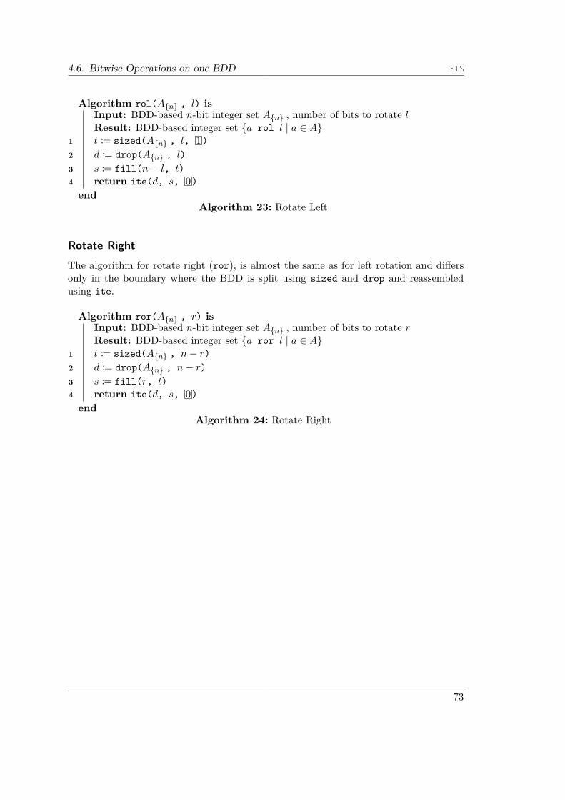
4.6. Bitwise Operations on one BDD

Algorithm rol(A{n} , l) isInput: BDD-based n-bit integer set A{n} , number of bits to rotate lResult: BDD-based integer set {a rol l | a ∈ A}

1 t := sized(A{n} , l, 1)2 d := drop(A{n} , l)3 s := fill(n− l, t)4 return ite(d, s, 0)end

Algorithm 23: Rotate Left

Rotate RightThe algorithm for rotate right (ror), is almost the same as for left rotation and differsonly in the boundary where the BDD is split using sized and drop and reassembledusing ite.

Algorithm ror(A{n} , r) isInput: BDD-based n-bit integer set A{n} , number of bits to rotate rResult: BDD-based integer set {a ror l | a ∈ A}

1 t := sized(A{n} , n− r)2 d := drop(A{n} , n− r)3 s := fill(r, t)4 return ite(d, s, 0)end

Algorithm 24: Rotate Right

73

4. BDDStab Library

4.7. BDDStab Library Implementation

The BDDStab library (Chapter 4) implements BDD-based integer sets (Sections 4.1,4.2), as well as transfer functions on these sets (Section 4.4 to 4.6). With it, we targetinteger value analyses that are implemented on the Java platform, i.e., that are executedon the Java Virtual Machine (JVM). To use pattern matching on BDDs, which we believenot only simplifies the implementation of our library but also makes the code readable,we chose Scala as our implementation language. With Scala, the library consists ofabout 4000 lines of code. Since Scala provides language constructs that Java does not,we provide Java compatible APIs whenever needed.

Different integer analyses require different abstractions. It is common for most lan-guages to only support a limited set of integer types with constant bitwidth, such asint or long. For the analysis of these languages, it is sufficient to provide a set ab-straction that can only handle exactly these types, i.e., a BDD-based set supportingconstant bitwidth integers. However, there exist languages that support integers ofvarying bitwidth, which demands a set data structure that can support these. In Jak-stab, each integer is a combination of a bitwidth and a bitvector, where the bitwidthdetermines where overflow happens in additions.

We therefore provide different entry points to our BDD-based integer sets, all withassociated transfer functions. Figure 4.11 shows an overview of these entry points. Inthis figure, the arrow denotes composition, i.e., CBDDs are a wrapper around BDDs,IntSets wrap CBDDs, and IntLikeSets wrap IntSets. Most algorithms are defined on theCBDD class, as it represents reduced BDDs with labelless nodes and complementableedges. IntSets and IntLikeSets are integer sets that implement Scala’s set trait. Thedifference between them is that IntSets only supports integers with constant bitwidth,while IntLikeSets supports integers with dynamic bitwidths as required by Jakstab.

In Sections 4.7.1 to 4.7.4, we provide more details for each of the library’s entry pointsand give an overview of their APIs. We finish with a description of our test suite inSection 4.8.

BDD

CBDD

IntSet

IntLikeSet

Figure 4.11.: Main Hierarchy in BDDStab Library

74

4.7. BDDStab Library Implementation

4.7.1. The BDD Class

The BDD class implements BDDs with complement edges, but without the complementinformation that applies to the root of a BDD. Therefore, this class only represents thepart of a BDD with complemented edges that is shared using a unique table [56].

One of the challenges when implementing a BDD package is to enforce the BDD’sreduction rules. With labelless BDDs, we have to remove redundant sub-BDDs, andreplace a decision node by one of its sub-BDDs if both sub-BDDs are the same termi-nal. We implement both reduction rules in a factory for decision nodes, require thatall non-terminal BDDs are built using it, and provide static objects for the terminal.Implementing Rule 1 from Section 4.1.1 is done by only creating a new decision node ifnot both sub-BDDs are the same terminal. If they are, then the factory returns one ofthem.The factory’s implementation of Rule 2 from Section 3.9 is done using hash consing,

which ensures that each BDD exists at most once in memory. Hence, if two BDDs areequivalent, they are the same object. Hash consing exploits that both argument sub-BDDs have been constructed using the factory, and must therefore be reduced already.The implementation uses a unique table that stores the forest of BDDs that have previ-ously been constructed. If the BDD that the factory must build exists in the forest, thenthis BDD is returned. Otherwise, a new BDD is constructed and added to the forest. Toenable fast lookup in the forest, we use a weak hashmap, which requires fast hash com-putation and equality checking between BDDs. As is common in hash consing, we makethe hash of a decision node dependent only on the hashes of its sub-BDDs, and storethe hash of each BDD in its root, thus avoiding recursion. When constructing a decisionnode with sub-BDDs A and B, the factory creates a hash for (A ◦ B), and accesses thecorresponding bucket in the hashmap. Within this bucket, the factory searches for theBDD (A ◦ B), using the O(1) reference equality on A and B that is established by hashconsing, and returns it if it exists. Otherwise, the factory creates a new decision node,adds it to the hashmap and returns it.The BDD class itself is not intended to be used outside of its wrapper class CBDD,

which we present next.

4.7.2. The CBDD Class

The CBDD class implements labelless BDDs with complemented edges, and O(1) satis-fiability count as described in Section 4.1. To simplify the use of CBDDs, we provide anAPI that transparently handles the complement bits, as well as the machinery for thesatisfiability count and acts as a simple binary tree with Booleans at the leaves.The API addresses two concerns: construction and deconstruction. Construction of a

CBDD is done using either a terminal node, available via the objects True and False inScala, and True$.MODULE$ and False$.MODULE$ in Java, or via creating a decision nodegiven two CBDDs. The construction of a decision node with true successor BDD T andfalse successor BDD F is done using Node(T, F) in Scala, and Node$.MODULE$.apply(T,F) in Java. Deconstruction, i.e., extracting the true and false successor BDDs from a

75

4. BDDStab Library

BDD, is done using pattern matching agains Node(a, b) in Scala, where a will beassigned the true successor BDD, and b the false successor BDD. In Java, one usesthe Node$.MODULE$.unapply method that returns an optional tuple of true and falsesuccessor BDDs. This optional value is empty, if the given BDD cannot be deconstructed,i.e., when it is a terminal.Additionally, CBDDs contain static methods, e.g., for the if-then-else function on

BDDs and BDD evaluation, the construction algorithms described in Section 4.3, andthe transfer algorithms from Sections 4.4 to 4.6. The presence of these algorithms on theCBDD level facilitates the implementation of new BDD-based integer set data structuresfor value analysis.

4.7.3. The IntSet ClassIntSets implement BDD-based integer sets for any finite integral type with a constantfinite bit length, such as Integer and Long. Only integer types that support certainfunctionality can be used with Intsets. These types must be integral, i.e., support com-mon operations on integers such as addition, negation, multiplication and comparison,and must be representable using a constant size bitvector. These type constraints areimplemented using Scala type classes, implementations of which must be passed duringIntset construction. The BDDStab library provides implementations for Java’s Integerand Long types.

The API supports IntSet creation via the overloaded method IntSet in Scala, andIntSet$.MODULE$.apply in Java. This method can construct IntSets from Scala integersets, Java integer sets as well as intervals.

4.7.4. The IntLikeSet ClassIntLikeSets implement BDD-based integer sets for integers up to a finite bitwidth, i.e.,finite integers. Additionally to the requirements for IntSets, IntLikeSets require theincluded type to support an operation that returns their bitwidth, as well as one thatconverts them into a constant bitwidth type such as Long. This abstraction allows us tohave the API deal with Jakstab numbers (RTLNumbers) directly instead of convertingin the Jakstab Adapter.Creation of IntLikeSets is done similarly to that of IntSets, i.e., via an overloaded

IntLikeSet method in Scala, named IntLikeSet$.MODULE$.apply in Java. Since theScala methods require passing of type class implementations, we provide special con-struction methods for Java’s Long type so that no passing of type class implementationsis necessary in this case.

4.8. TestingThe BDDStab library contains about 60 ScalaCheck tests, testing not only the set typesfor basic functionality such as adding elements to the set and checking for membership,but also the implementation of all algorithms from Sections 4.3 to 4.6 with particular

76

4.8. Testing

focus on algo, add, and mulSingl. These tests are formulated as functions that, givenappropriate input data, return true exactly when the implemented test case succeeds.ScalaCheck generates pseudo random input, and calls the tests with it. Most of our testsuse an oracle, i.e., a simple but inefficient implementation of an algorithm using explicitsets that predicts the correct result. To facilitate the implementation of such oracles forIntLikeSets, the BDDStab library includes a class for integers with a dynamic behavior,i.e., arbitrary bitwidth and corresponding wrap-around.

77

4. BDDStab Library

4.9. EvaluationWe evaluate the performance of the BDDStab library on integer sets that have exactrepresentations in the common abstractions of integer sets. If these experiments revealthat BDD-based integer sets are suitable for the exact representation of these shapes,then it is likely that they are also suitable for the representation of integer sets that areclose to these representations, as the BDD shape will not change drastically by adding ordeleting a few elements. In particular, we evaluate the following two set shapes, knownfrom other value analyses:

1. Intervals

2. Congruence Classes

For intervals, we evaluate the efficiency of the BDD representation, and for congrunececlasses, we additionally evaluate the construction speed, and the performance of the pre-cise algorithms for abstract evaluation, namely addition and binary bitwise operations.

4.9.1. Measuring Procedure

To determine the efficiency of our BDD-based integer representation and measure theperformance of algorithms, we record the following measurements:

1. The number of decision nodes in unique sub-BDDs

2. The number of decision nodes in all sub-BDDs

3. Time spent during execution of an algorithm

Measurement 2 is the number of decision nodes a labelless BDD would include ifequivalent sub-BDDs would not be shared. We call the BDD that would result fromnot sharing equivalent sub-BDDs binary decision tree (BDT). This number is computedduring node construction and is therefore easily available. Only Measurement 1 is notavailable and must be computed. Since we use maximal sharing via hashconsing (Section4.7.1), we compute this number by constructing the BDD we want to measure, thenrequest the garbage collector to run, wait and query the number of elements in the uniquetable that stores all unique sub-BDDs. Before construction and after measurement weclear the unique table. Requesting and waiting for the garbage collector is necessaryto purge the weak hashmap that implements our unique table of decision nodes thatwere only constructed temporarily and are not part of the final result. Because onlydecision nodes are stored in the unique table, this measurement does not include theterminal node. Measurement 1 provides insight into the nodes our BDD-based integerset implementation uses in total to represent integer sets, while the relation betweenMeasurement 2 and 1 shows the effectiveness of sharing equivalent sub-BDDs within oneBDD. Note that sharing increases its effectiveness with a growing forest. To measure

78

4.9. Evaluation

the speed of our algorithms, we used an early 2015 MacBook Pro with a 3.1 Ghz i7processor and 16 GB of DDR3 ram.

In the evaluation of the algorithms for abstract evaluation, we use Measurement 3,i.e., the time spent computing results for a representative subset of a given set shape. Asan example, to evaluate the addition algorithm on intervals, we choose a representativesubset of intervals, apply the addition algorithm on all elements in this subset andmeasure its execution time. Note that we do not instruct the garbage collector to runwhen evaluating algorithm performance, since our algorithms make use of caching toimprove performance, and the garbage collector may clear the caches, hence negativelyaffecting algorithm performance.

4.9.2. Representation Efficiency for IntervalsTo evaluate the efficiency of our BDD-based integer set data structure when representingintervals, we construct all 10-bit intervals, represent them with BDD-based integer sets,and record Measurement 1. Using 10-bit intervals results in 210∗210/2 = 524288 intervals,since there exist 210 possible lower and upper bounds, giving 220 possible combinationsof lower and upper bounds, half of which have a lower bound that is smaller or equalto the upper bound. Measuring all 11-bit intervals would already have required about2 million measurements, which would have required an excessive amount of time. Sincewe spend most of the time waiting for the garbage collector to run, we cannot increasethe benchmark speed by using more powerful hardware. Hence, 10-bit intervals is agood compromise between a speedy execution of the benchmark and a representativebitwidth, i.e., one that is wide enough to reveal the behavior of the BDDs on largerbitwidths.Figure 4.12 shows a histogram of the reduced BDD sizes for all 10-bit intervals. The

x-axis shows Measurement 1, i.e., the number of nodes in the reduced BDD, and they-axis denotes how often this number was measured in logarithmic scale. We observethat the BDD size varies between 23 and 44 nodes, with an average number of 36 nodes.It may be surprising that we observe BDD sizes greater than twice the bitwidths of the

represented intervals, since an n-bit interval is represented by two n-bit numbers. Thisoddity is explained by the fact that we use the bitwidth of an underlying type internally.In the interval measurements, we used Java Integer, i.e., 32-bit as underlying type,meaning that only the last 10 bits of the BDDs represent the intervals, while the upper22 bits are set to 0. Hence, the theoretical maximum BDD size for 10-bit intervals is 42because there are 32− 10 = 22 bits outside of the 10 bit used to represent the intervals,and 2 ∗ 10 bits are used for the two interval boundaries. However, the data contains asample where the maximum measured result is 44, i.e., 2 over the theoretical maximum.Closer investigation reveals that this is the only test case where the number of nodes inthe BDT form is smaller than that of the reduced BDD form (44 > 23). Recreation ofthis interval and waiting for garbage collection showed the real number of reduced BDDnodes to be 23. Hence, the result of this test case is an artifact.With a theoretical maximum BDD size of 2n+c−n, when representing n-bit intervals

in an underlying c bit integer type, where c is usually 64, the size of BDDs representing

79

4. BDDStab Library

intervals remains small. Better yet, further investigation of our benchmark data revealsthat sharing equivalent sub-BDDs improves the average BDD size by about 14%, evenwhen representing intervals, which only demand storing two numbers and therefore leadto a simple BDD shape.

Figure 4.12.: Node Count of Reduced BDD Representing 10-bit Intervals

4.9.3. Representation Efficiency for Congruence Classes

Compared to n-bit intervals, where the BDD representation must at most store twon-bit paths, congruence classes produce BDDs with more internal nodes, as they arenon-convex and hence must represent holes between any two included elements. There-

80

4.9. Evaluation

fore, representing congruence classes using BDD-based integer sets is more challenging,and hence we provide a more in-depth evaluation that covers the effectiveness of reduc-tion Rule 1 from Section 4.1.1 (Measurement 2) as well as the performance of variousalgorithms (Measurement 3). We use Algorithm 6 to construct integer sets with dynamicbitwidth set to 16, and the underlying constant bitwidth 32, for all possible strides. Intotal, we therefore measure 216 − 1 = 65535 BDD-based integer sets, since 0 is not avalid stride. We chose 16 bit, as it is a common integer size and still small enough toallow measuring all possible congruence classes. In difference to intervals, which aredefined by two parameters, i.e., upper and lower bound, and are therefore hard to plotin two dimensions, congruence classes are defined by one parameter only, i.e., the stride.Hence, we will not use histograms, as we did for intervals, but instead use a regulartwo-dimensional plot.

Figure 4.13 shows our measurements with the stride on the x-axis in logarithmic scale,and the number of nodes in the reduced BDD on the y-axis. The node count for thereduced BDDs ranges from 16, at stride 1, to 780 for stride 257, and is 77 in average.

It may be surprising that the minimum size of the reduced BDD is 16 and not 0,as stride 1 should generate 1 as BDD, which is not measured because it is a terminal.Similarly to the interval benchmark, the first 32 − 16 = 16 bits are set to 0 in ourimplementation. Hence, 16 is the least number of nodes possible for any non-empty16-bit integer sets, represented using an underlying 32 bits in the BDD. Apart from theleft most point, corresponding to stride 1, the strides producing the smallest BDDs are2n strides, which is not surprising because in these strides, the last n bits of all includedelements and, therefore, their BDDs are constant. Figure 4.13 shows several sub-plotsthat behave similarly, i.e., they rise to their peak, and then fall again. We call each ofthese sub-plots a stride class, distinguish them using color, and number them as givenin the legend. Closer investigation reveals that each stride can be assigned to exactlyone stride class as it fulfills s%2c == 2c−1, where s is the stride and c the stride classnumber, only for exactly one class number. As an example, consider the stride classwith the highest peak (outer, enclosing plot). All strides s in this stride class satisfys%2 == 1, i.e., the strides are all odd. Similarly, the next lower stride class are builtfrom strides s with s%4 == 2. From the classes, we can conclude that the lower thestride class, the less efficient is the BDD representation.The shape of the stride classes,i.e., rising quickly in the beginning then falling off, confirms our expectation about theperformance of Algorithm 6: Small strides lead to more sharing (memoizing), while largestrides lead to small sets. Both, sharing and small set sizes, can produce minimal BDDs.

The average 77 nodes required to represent 16-bit congruence classes within reducedBDDs with 32 variables is encouraging, especially when considering that the congruenceclass with stride 2 would have 216 nodes without sharing.

81

4. BDDStab Library

Figure 4.13.: Node Count for all 16-bit Strides in 16-bit Integer Sets

To investigate further the efficiency of BDD reduction when representing congruenceclasses, we next show the relation between the node count of BDTs (Measurement 2)to that of the reduced BDDs (Measurement 1), i.e., we show the factor by which thereduced BDD contains fewer nodes than the non-reduced BDT. Figure 4.14 containsthe plot of the relation, again for all 16-bit congruence classes, with the stride on thelogarithmic x-axis, and the relation on the y-axis. We see that the BDD and BDT sizesare essentially equal for stride 1. The reason for equality in this case is that stride 1 leadsto a full set of all 16 bit integers, which is represented by just 1 for the reduced BDDand the BDT that implements only reduction Rule 2. The most efficient representationof each stride class is at a power of 2, since the bitvectors contained in the BDDs have

82

4.9. Evaluation

constant trailing zeros. As an example, the congruence class of 4-bit integers with stride4 contains 0, 4, 8, and 12, all of which have the two least significant bits set to 0.Above these constant bits, the stride class will contain all bit patterns, which results inan efficient BDD representation. Unsurprisingly, the stride class with the highest nodecount (Class 1 in Figure 4.13) has the least efficient BDD representation.

Figure 4.14.: Ratio between Number of Nodes in Non-Reduced and Reduced BDDs forall 16-bit Strides in 16-bit Integer Sets

83

4. BDDStab Library

Construction Performance for Congruence Classes

Figure 4.15 shows the construction times, i.e., Measurement 3, of congruence classeswhen using Algorithm 6 to construct all congruence classes of 1- to 24-bit integers.For each bitwidth n, we construct all congruence classes with the strides from 1 to2n − 1, meaning we create up to 224 − 1 sets for one measurement. The x-axis showsthe bitwidth of the created congruence classes, the y-axis shows the time in seconds ittook to create all congruence classes of the given bitwidth, and the color indicates themaximum construction time of one congruence class of the given bitwidth. Note thatthe scale of the construction time (y-axis) is logarithmic.

Figure 4.15.: BDD Construction Speed for all Strides in 1- to 24-bit Integer Sets

84

4.9. Evaluation

We observe that the construction of all 1-bit congruence classes, which is only the set{0, 1}, takes unusually long. We consider this measurement an outlier, most likely causedby the Java runtime system’s optimization procedure. It is noticable that, particularlyafter the 12-bit congruence class constructions, the construction time increases linearlyin the logarithmic scale. This progression is not surprising, as we always construct allpossible congruence classes and the number of possible congruence classes with offset 0in n-bit integers is 2n. Hence, we call the construction algorithm 2n times for each datapoint, which suggests that the construction times grow linearly with the bitwidth of theconstructed congruence class. The maximum construction times of single congruenceclasses per bitwidth ranges from 1 millisecond to 34 milliseconds when ignoring theoutlier for bitwidth 1. We would expect the maximum single construction time, whenignoring the outlier at 1, to occur at the widest bitwidth, but instead, we measured itat bitwidth 22, which suggests that there is jitter on the measurements. This jitter can,e.g., be caused by the garbage collector.

Algorithm Performance for Congruence ClassesThe previous benchmarks have shown that our BDDs efficiently represent congruenceclasses by sharing common sub-BDDs, which leads to smaller reduced BDDs. However,smaller BDD sizes do not necessarily improve the performance of the algorithms thatoperate on them. Ignoring memoization, algorithms are defined on the BDT form, andwe have shown that there may be huge differences between this non-reduced form and thereduced form. We therefore evaluate the performance of the exact algorithms for binarytransfer functions, namely the addition algorithm (Algorithm 11), and the algorithm forbinary bitwise operations (Algorithm 8) on BDD representations of congruence classes.Since we expect the same performance for any of the common bitwise operators (∨ and∧ on the bit level), we only present data for bitwise and.Similarly to the measurements on intervals, we chose 10-bit congruence classes, because

we want to evaluate the performance of the algorithms on all unique combinations of alln-bit congruence classes, and that leads to 22n measurements. For 10-bit, we thereforehave to record about 1 million samples, which is acceptable.

Figure 4.16 shows the time (Measurement 3) needed by the addition algorithm whenadding two 10-bit congruence class sets, while Figure 4.17 shows the same for the logicaland. As we can see, their performance is almost equivalent. The maximum time spentfor one operation is about 1 second for both. However, the mean of all additions is atabout 4 milliseconds, while the mean of all bitwise operations is about 3 milliseconds.All but two additions took less than 550 milliseconds, and all but two bitwise operationstook less than 750 milliseconds. Since our measurements contain Java runtime actions, itis possible that the two outliers are caused by garbage collector runs. Further inspectionof the data did not reveal that the performance of the algorithms is significantly betteror worse for specific congruence classes.

Even though speeds close to 1 second may be excessive for the application of onetransfer function, the vast majority of cases show a performance of under 4 milliseconds,which is acceptable, considering that both algorithm produce an exact result.

85

4. BDDStab Library

Figure 4.16.: Addition of all Combinations of all 10-bit Congruence Classes

86

4.9. Evaluation

Figure 4.17.: Bitwise And of all Combinations of all 10-bit Congruence Classes

87

4. BDDStab Library

4.9.4. Threats to ValidityWe identify two potential threats to the validity of our data:

1. Dirty computed table

2. Tested bitwidths not representative

Threat 1 threatens our measurements because we use System.gc() to clean our com-puted table of non-referenced BDDs and this only suggests to the Java Virtual Machine(VM) that garbage collection may be beneficial, it does not necessarily cause the VMto perform garbage collection. If the production of the BDDs that must be measuredcauses the creation of temporary BDDs which are not part of the BDD that should bemeasured, and these temporary BDDs are not dropped by the garbage collector, then themeasurement of the number of decision nodes of the BDD will include spurious nodes.A dirty computed table, however, can only lead to pessimistic values, i.e., to an

overestimation of the reduced BDD size. Therefore, the values we report for the reducedBDD sizes must be interpreted as an upper bound, not as the exact size.

Threat 2 may invalidate the conclusions we draw from the measurements as we onlytested the BDD sizes for sets of fixed bitwidths. This threat cannot entirely be dis-missed. However, we find it unlikely that effects that occur in a certain bitwidth do notoccur on wider or narrower sets and vice versa. To double check, we ran a selectionof our benchmarks with narrower and wider bitwidth and found the same phenomena,suggesting that our selection of bitwdiths are representative.

88

5. JakstabIn Chapter 2, we motivated that reconstructing control flow is the focal task in theanalysis of executables, and that this task involves resolving jump targets, which in turndemands the computation of possible sets of integers for the target addresses. Jakstab,a static analysis framework for x86 32-bit executables created by Johannes Kinder [3],provides all the necessary machinery for the flow-based analysis of executables, suchas parsing the executable (e.g., ELF or EXE), as well as an implementation of CPA.CPA enables the formulation of an analysis on a dynamically constructed control flowgraph, facilitates the implementation of disjunctive refinement via the merge operator,and improves precision via the combination of analyses.In Jakstab, we distinguish between four different abstract entities: Abstract value,

abstract environment, abstract location, and abstract state. An abstract value is arepresentation of a concrete value, e.g., a representation of Booleans or Integers, whilean abstract environment represents an assignment of all storage locations to an abstractvalue. An abstract location represents a control position in the analyzed program, andan abstract state is the combination of an abstract location and abstract environment. Ingeneral, entities in the concrete are singletons, while their abstract counterparts describea collection of concrete values. As an example, X86 registers may each contain only onebitvector, while in the abstract, each register is associated with a set of bitvectors.Jakstab draws its strengths from its plug-ins, which implement the core part of the

analysis, and communicates with its plug-ins via its intermediate language SSL. Hence,plug-ins must not only support the operators required by CPA, such as merge, stop, andconcretization, but also abstract evaluation and transfer functions for all SSL statementsand expressions. Soundness requires that these functions are overapproximating (seeChapter 3.5). Jakstab’s analysis process is visualized in Figure 5.1. Jakstab keeps aset of active abstract states in the workset and extracts one such state in each analysisiteration. It deconstructs this state into a location in the executable and an abstractenvironment, lifts the instruction found at the location to SSL, and calls the analysisplug-in with the resulting SSL and the abstract environment. The active abstract states,computed by the plug-in, are added back to the workset and the next analysis iterationis started.In the remainder of this section, we focus on integer value analysis, i.e., abstract values

are sets of n-bit integers.

5.1. Value Analysis with JakstabImplementing an integer value analysis plug-in for Jakstab requires the implementationof the abstract environment, abstract values, and transfer and evaluation functions forSSL statements and expressions respectively. In Figure 5.1, a new value analysis plug-inwould therefore provide the “Environment” as well as the “Analyze” parts in Jakstab’sanalysis flow. In Jakstab, abstract locations are hidden from value analysis plug-ins,which therefore operate on abstract environments instead of abstract states. Jakstab

89

5. Jakstab

Workset Abstract State

Location Lift

Environment

Analyze

Figure 5.1.: Jakstab Analysis Process

computes the corresponding abstract locations either by using the length and locationof the analyzed expression in case of a non-jump instruction, or by calling the abstractevaluation function with the produced abstract environment on the target address of ajump.

In the following sections, we will first focus on the abstract environment (Section5.2), and then present Jakstab’s intermediate language (Section 5.3). Afterwards, inChapter 6, we describe our BDDStab Jakstab adapter, which uses the BDDStab libraryto implement BDD-based value analysis for Jakstab.

5.2. Abstract Environment

To define a common abstract environment for a value analysis in Jakstab, let us firstconsider the shape of a concrete environment as depicted in Figure 5.2. Formally, a stateis a combination of a program location together with an environment, i.e., an assignmentof each storage location to a value. In the following, we focus on the environment, asthe location is part of Jakstab’s location CPA and must therefore not be reimplementedby a value analysis plug-in. Further, we only consider integral values, as it is uncommonfor floating point values to be converted to integral values and used in indirect jumps. Aconcrete environment consists of a RegTable, which is a function that assigns a value toeach register, as well as a Heap, which assigns a value to each address. It is possible thatthere is no meaningful value for a register or memory location, as none might have beenassigned. In an actual execution on a computer, accessing this location would most likelyyield a random value, a behavior which can be captured in the abstract by initializingthat memory location with >.An abstract environment, as visualized in Figure 5.3, is structurally equivalent to a

concrete environment, with concrete integral values replaced by abstract values, whichsummarize a set of concrete values soundly. While in the concrete, associations betweenstorage locations and values can be modeled by simple updatable associations, modelingHeap and RegTable in the abstract is slightly more complex.

90

5.2. Abstract Environment

EnvironmentRegTable

Heapi ∈ Z

Register

Address

Figure 5.2.: Concrete Environment

Abstract EnvironmentRegTable

HeapAbstract Value (AV)

l ⊆ region× Z

γα

Register

AV

Figure 5.3.: Abstract Environment

Heap

Jakstab’s heap model supports abstract base addresses, called regions, which are gener-ated by memory allocation statements. Additionally there always exists a global regionthat is used by default, e.g., when no dynamic memory management is used or the useof dynamic allocations cannot be identified in the executable. The set of possible regionsforms a join semi-lattice, hence a top symbol exists, which signifies that a region couldnot be determined precisely. Since it is not possible to distinguish pointers from integerson the binary level, all integers are assigned the global region by default, which signifiesa base address of zero. It is assumed that abstract regions cannot overlap. Therefore, ifan operand address of a memory operation cannot be computed precisely enough or isapproximated to >, then the region information may limit the effect of the operation tothe region only. The core difference between the operation of the Heap in the concrete isthat there, values are singletons. In the abstract, each value represents a set of concretevalues. Therefore, the Heap must support lookup and write operations on collectionsof addresses. Since these collections of addresses are overapproximations, it cannot beguaranteed that a write operation deletes information stored before under the given ad-dresses. Only when the collection of target addresses for a write operation is a singletoncan old information at that address be deleted safely, since even if this singleton wouldbe spurious, execution in the concrete would not be able to perform the write operation.

RegTable

In difference to the Heap, the RegTable is not addressable, so that values cannot beaccessed using computed values. Instead, values are accessed using constant registernames. Therefore, write operations can always overwrite present information. X86 hasregisters that overlap by default, e.g., there are 8- and 16-bit sized registers that containparts of an underlying 32-bit register.

91

5. Jakstab

5.3. Intermediate LanguageSimilar to other analysis frameworks [33, 74, 75], Jakstab uses an intermediate languageto perform the analysis on. Whenever an analysis has determined a new program locationas reachable, Jakstab lifts the instruction at that location to the intermediate languageand performs a new analysis step which produces new successor states, which in turncontain successor locations. The iterative process of lifting and analysis continues atthese new successor locations, and since the successor locations are computed as partof the analysis, the precision of the computed control flow depends on the analysis aswell. However, the control flow analysis itself is hidden from the value analysis partand therefore this part does not have to handle control flow instructions such as jumpsexplicitly.In Figure 5.4, we present those instructions that are exposed to the value analysis part

of the analysis, such as BDDStab. The instructions can generally be categorized intoexpressions that operate on abstract values, and statements that operate on abstractstates. For expressions, Jakstab plug-ins must provide evaluation functions that takeabstract values and produce abstract values that correspond to the result. The trans-fer functions for statements use these evaluation functions to soundly update affectedvariables and memory locations corresponding to the statement.Our BDDStab Adapter supports the underlined statement and expression types from

Figure 5.4, which we describe in Table 5.1.

92

5.3. Intermediate Language

〈Program〉 |= 〈Statement〉 ∗

〈Statement〉 |=

〈VarAssignment〉 | 〈MemAssignment〉| 〈Assume〉 | 〈Alloc〉| 〈Dealloc〉 | 〈UnknownCall〉| 〈Havoc〉 | 〈MemSet〉| 〈MemCpy〉

〈Expression〉 |=

〈BitRange〉 | 〈CondExpr〉| 〈MemLoc〉 | 〈Nondet〉| 〈Number〉 | 〈Operation〉| 〈SpecialExpr〉 | 〈Variable〉

〈Operation〉 |=

〈Expression〉 == 〈Expression〉| 〈Expression〉<〈Expression〉| 〈Expression〉≤〈Expression〉| 〈Expression〉<u〈Expression〉| 〈Expression〉≤u〈Expression〉| !〈Expression〉| -〈Expression〉| 〈Expression〉&&〈Expression〉| 〈Expression〉||〈Expression〉| 〈Expression〉^〈Expression〉| 〈Expression〉+〈Expression〉| 〈Expression〉*〈Expression〉| 〈Expression〉/〈Expression〉| 〈Expression〉%〈Expression〉| 〈Expression〉>>>〈Expression〉| 〈Expression〉>>〈Expression〉| 〈Expression〉<<〈Expression〉| 〈Expression〉rol〈Expression〉| 〈Expression〉ror〈Expression〉

〈VarAssignment〉 |= 〈Variable〉 := 〈Expression〉〈MemAssignment〉 |= 〈MemLoc〉 := 〈Expression〉

〈Assume〉 |= assume(〈Expression〉)〈Variable〉 |= %[a-c]+〈Number〉 |= %[0-9]+〈MemLoc〉 |= M(〈Expression〉)〈BitRange〉 |= bitRange(〈Expression〉, 〈Expression〉, 〈Expression〉)〈CondExpr〉 |= 〈Expression〉?〈Expression〉 : 〈Expression〉〈Nondet〉 |= nondet

Figure 5.4.: Fragment of Jakstab’s IL relevant for Value Analysis

93

5. Jakstab

VarAssignment Updates the given variable to the value of the given expressionMemAssignment Updates the value stored at the given address to the value of the

given expressionAssume Prevents execution to continue if given expression evaluates to

falseBitRange Slices a given integer on the bitlevelCondExpr Evaluates to the second expression if the first is true and to the

third otherwiseMemLoc A heap location described by the given addressNondet An arbitrary valueOperation Boolean, arithmetic, or bitwise operationNumber A numberVariable A variable== True exactly when both operands are equal< True exactly when first operand is strictly smaller than second in

signed interpretation≤ True exactly when first operand is smaller or equal to second in

signed interpretation<u True exactly when first operand is strictly smaller than second in

unsigned interpretation≤u True exactly when first operand is smaller or equal to second in

unsigned interpretation! Bitwise or Boolean negation− Arithmetic negation& Bitwise or Boolean and|| Bitwise or Boolean orˆ Bitwise or Boolean xor+ Addition∗ Multiplication/ Division% Modulo>>> Bitwise shift right>> Arithmetic shift right<< Shift leftrol Rotate leftror Rotate rightnondet Non-deterministic value

Table 5.1.: Description of Expressions, Statements, and Operations relevant for ValueAnalysis

94

6. BDDStab Jakstab Adapter

In the previous chapter, we introduced the Jakstab framework for binary analysis andits requirements for value analysis CPAs in the form of plug-ins. In this chapter, weuse the BDDStab library (Chapter 4) in the implementation of such a plug-in. Besidesthe merge and stop operators, we define the transfer and abstract evaluation functions(Sections 6.1, and 6.2 respectively) on the intermediate language SSL, which provide theheavy lifting of the plug-in. The most intricate transfer function is the assume statement,which makes our analysis path-sensitive by producing precise restrictions for the true andfalse successors of conditional branches. To improve precision of this transfer function,we define an overapproximating constraint solver (Section 6.3) and an equivalence classanalysis (Section 6.4) that enables the restriction of related storage locations that arenot directly mentioned in the condition. Lastly, we briefly discuss widening (Section 6.5)and tie the presented analysis parts together to a CPA instance in Section 6.6.

6.1. Statements

In this section, we discuss the transfer functions for the statements of the intermediatelanguage as presented in Figure 5.4. In the definitions, we assume an abstract evalu-ation function eval, which evaluates a given expression e in a given abstract state σ#

(evalJeK(σ#)). We describe the eval function in Section 6.2.The transfer functions for the statements are as follows, where the subscript in the

brackets denotes the statement type:

fBDD[α:=e](σ#) = σ#.r[α] := evalJeK(σ#)

fBDD[M(e1):=e](σ#) =

σ#.h[m] := evalJeK(σ#) if {m} = evalJe1K(σ#)⊔{σ#.h[m] := σ#.h[m]tevalJeK(σ#) | m ∈ evalJe1K(σ#)}

otherwise

fBDD[assume(e)](σ#) = σ# u solveoJeK(σ#)

The transfer function for the variable assignment updates the register table at theposition described by α to the result of the evaluation function on e in σ#. In principle,the transfer function for variable assignment is similar to the transfer function for heapassignment. There is, however, a noticable difference: The evaluation function for theassignment to the heap only updates, and thereby deletes, the old value if its addresscan be resolved without ambiguity, i.e., can be resolved to a singleton set. If the heapaddress cannot be resolved to a singleton, then the transfer function does not perform adestructive update and joins the new with the old abstract values instead (weak update).The function is limited to weak updates in case the heap address cannot be resolved to asingleton, because the abstract evaluation function, applied to the expression providingthe address, computes an overapproximated result, meaning that not each of the elementsfrom the concretization of the set may be assumed to be feasible. Therefore, it cannot be

95

6. BDDStab Jakstab Adapter

assumed that an update at a specific address occurred or not. The situation is differentif the set of heap addresses is a singleton: Even though this singleton value could bethe result of an overapproximation, and therefore have no feasible concretization, strongupdate is sound, since control could not reach the heap assignment in the concrete. Wedelay the discussion of the assume statement until Section 6.3.

6.2. Abstract Evaluation FunctionIn this section, we will use the algorithms provided by the BDDStab library to definethe abstract evaluation function evalJeK(σ#). We assume that constants are denoted byc, variables by v, and memory locations by M(e), and split the definition of the abstractevaluation function into 5 categories:

1. Constants, registers, memory locations, and Boolean and arithmetic negation (Fig-ure 6.1)

2. Relational operations (Figure 6.2)

3. Binary bitwise and arithmetic operations (Figure 6.3)

4. Shifts and rotations (Figure 6.4)

5. Bit-level slicing, conditional expression, and non-determinism (Figure 6.5)

evalJcK(σ#) = fromNumber(c, 0, 0, 1)evalJvK(σ#) = σ#.r[v]evalJM(e)K(σ#) = ⋃

{σ#.r[c] | c ∈ evalJeK(σ#)}evalJ!eK(σ#) = not(evalJeK(σ#))evalJ−eK(σ#) = negate(evalJeK(σ#))

Figure 6.1.: Abstract Evaluation for Constants, Registers, Memory Locations, andBoolean and Arithmetic Negation

The abstract evaluation function for relational operators (Figure 6.2) returns 0 , i.e.,⊥ for BDD-based integer sets, when the evaluation of either of the operands evaluates to0 . Returning 0 in this case is correct, because in the concrete, evaluation of a booleanexpression must yield either true or false, and if overapproximated evaluation yields0 , then execution cannot reach this program point. For ==, the abstract evaluationfunction returns (0 ◦ 1), i.e., the abstraction of false, when there does not exist a valuethat is in the evaluation of both expressions. Similarly, it returns (1 ◦ 0), i.e., theabstraction of true, when the evaluation of both operands is the same singleton, as then,there does not exist any combination of elements in the concrete that are unequal. In allother cases, i.e., the intersection of the operand evalutions is neither empty nor singleton,the evaluation function returns 1 , i.e., > for BDD-based integer sets. The remaining

96

6.2. Abstract Evaluation Function

relational operators from Figure 6.2 use the minimum and maximum functions to checkwhether there exist elements in the evaluations of the operands that fulfill either therelation or its negation, and add (1 ◦ 0), i.e., the abstraction of true, and (0 ◦ 1), i.e.,the abstraction of false, correspondingly.

evalJe1 == e2K(σ#) =

0 if evalJe1K(σ#) = 0 ∨ evalJe2K(σ#) = 0(0 ◦ 1) if evalJe1K(σ#) ∩ evalJe2K(σ#) = 0(1 ◦ 0) if {v} = evalJe1K(σ#) = evalJe2K(σ#)1 otherwise

evalJe1 < e2K(σ#) =

0 if evalJe1K(σ#) = 0∨evalJe2K(σ#) = 0⋃({(1 ◦ 0) | min(evalJe1K(σ#))

< max(evalJe2K(σ#))}∪{(0 ◦ 1) | min(evalJe2K(σ#))

≤ max(evalJe1K(σ#))})

otherwise

evalJe1 ≤ e2K(σ#) =

0 if evalJe1K(σ#) = 0∨evalJe2K(σ#) = 0⋃({(1 ◦ 0) | min(evalJe1K(σ#))

≤ max(evalJe2K(σ#))}∪{(0 ◦ 1) | min(evalJe2K(σ#))

< max(evalJe1K(σ#))})

otherwise

evalJe1 <u e2K(σ#) =

0 if evalJe1K(σ#) = 0∨evalJe2K(σ#) = 0⋃({(1 ◦ 0) | minu(evalJe1K(σ#))

< maxu(evalJe2K(σ#))}∪{(0 ◦ 1) | minu(evalJe2K(σ#))

≤ maxu(evalJe1K(σ#))})

otherwise

evalJe1 ≤u e2K(σ#) =

0 if evalJe1K(σ#) = 0∨evalJe2K(σ#) = 0⋃({(1 ◦ 0) | minu(evalJe1K(σ#))

≤ maxu(evalJe2K(σ#))}∪{(0 ◦ 1) | minu(evalJe2K(σ#))

< maxu(evalJe1K(σ#))})

otherwise

Figure 6.2.: Abstract Evaluation for Relational Operators

For multiplication in Figure 6.3, the evaluation function is defined for multiplicationby constants using mulSingl. The general case still uses mulSingl if evaluation of one

97

6. BDDStab Jakstab Adapter

operand yields a singleton set. Otherwise, we re-use the abstract multiplication functionfrom interval arithmetic (∗#[]) and the function bdd2ival, which overapproximates aBDD-based integer set by a set of covering intervals, and the function ival2bdd toconvert the resulting intervals back to BDD-based integer sets. The parameter p definesthe precision of the overapproximation and must be set appropriately. We use the samemethod to evaluate division, i.e., conversion from and to intervals and application of theinterval transfer function for division (/#[]).

evalJe1||e2K(σ#) = algo(evalJe1K(σ#), evalJe2K(σ#), ∨)evalJe1&&e2K(σ#) = algo(evalJe1K(σ#), evalJe2K(σ#), ∧)evalJe1 + e2K(σ#) = add(evalJe1K(σ#), evalJe2K(σ#))evalJe ∗ cK(σ#) = mulSingl(evalJeK(σ#), evalJcK(σ#))evalJc ∗ eK(σ#) = mulSingl(evalJeK(σ#), evalJcK(σ#))

evalJe1 ∗ e2K(σ#) =

mulSingl(evalJe2K(σ#), v1) if {v1} = evalJe1K(σ#)mulSingl(evalJe1K(σ#), v2) if {v2} = evalJe2K(σ#)⋃{ival2bdd(i1 ∗#[] i2) |

i1 ∈ bdd2ival(evalJe1K(σ#), p)i2 ∈ bdd2ival(evalJe1K(σ#), p)}

otherwise

evalJe1/e2K(σ#) =⋃{ival2bdd(i1/#[]i2) | i1 ∈ bdd2ival(evalJe1K(σ#), p)

i2 ∈ bdd2ival(evalJe1K(σ#), p)}

Figure 6.3.: Abstract Evaluation for Binary Bitwise and Arithmetic Operations

Abstract evaluation for shifts and rotations (Figure 6.4) is only supported if the eval-uation of the second operand yields a singleton. Otherwise, the abstract evaluationfunction returns 1 , i.e., > for BDD-based integer sets.

evalJe1 >>> e2K(σ#) ={

shiftr(evalJe1K(σ#), v2) if {v2} = evalJe2K(σ#)1 otherwise

evalJe1 >> e2K(σ#) ={

shiftrarith(evalJe1K(σ#), v2) if {v2} = evalJe2K(σ#)1 otherwise

evalJe1 << e2K(σ#) ={

shiftl(evalJe1K(σ#), v2) if {v2} = evalJe2K(σ#)1 otherwise

evalJe1 rol e2K(σ#) ={

ror(evalJe1K(σ#), v2) if {v2} = evalJe2K(σ#)1 otherwise

evalJe1 ror e2K(σ#) ={

rol(evalJe1K(σ#), v2) if {v2} = evalJe2K(σ#)1 otherwise

Figure 6.4.: Abstract Evaluation for Shifts and Rotations

The evaluation function for the bitRange expression (Figure 6.5) returns 1 , i.e., > for

98

6.3. Assume Statement

BDDs, if the lower and upper bit position cannot be resolved to a singleton. Otherwise,it calls the bitExtract algorithm with the computed bit positions. The evaluation ofthe ternary operator must include the evaluation of e2, if the evaluation of e1 includes 1,and the evaluation of e3 if the evaluation of e1 includes 0. The corresponding evaluationfunction implements this behavior by unioning a set of at most two BDDs, one for theevaluation of e1 and one for the evaluation of e3.

evalJbitRange(e1, e2, e3)K(σ#) =

bitExtract(V3) if

{v1} = evalJe1K(σ#)∧{v2} = evalJe2K(σ#)V3 = evalJe3K(σ#)

1 otherwiseevalJe1 ? e2 : e3K(σ#) = ⋃({evalJe2K(σ#) |

evalJe1K(σ#) = 1 ∨ evalJe1K(σ#) = (1 ◦ 0)}∪{evalJe3K(σ#) |

evalJe1K(σ#) = 1 ∨ evalJe1K(σ#) = (0 ◦ 1)})evalJnondetK(σ#) = 1

Figure 6.5.: Abstract Evaluation for Bit-level Slicing, Conditional Expressions and Non-determinism

6.3. Assume Statement

In this section, we discuss the handling of the assume statement. Jakstab generates thisstatement from conditional branches. As an example, consider the assembly programon the left-hand side of Figure 6.6. This program first loads into %ebx the contentsstored in the heap under an address given by %eax, and then compares it to 9. Ifthe comparison determines that the contents of %ebx is greater than 9, then the codejumps to $g using jg (jump greater). Otherwise the code jumps to $f using jle (jumpless or equal). In the abstract, a perfect transfer function would not only determinewhich transitions can be traversed in the given abstract state, but would also restrictthe storage locations affected by the condition accordingly. Considering the examplecode in Figure 6.6 and assuming that the variation domain of %ebx is an interval from 0to 20, the jump conditions of both jumps are determined as possibly true, whereas if theVD is 0 to 9, then only the transition to $f should be determined as possible. Assumingthat the address stored in %ebx can exactly be determined (its VD is singleton), theanalysis should derive that both %ebx and the abstract value stored under the addressin %ebx should be restricted to 0 to 9 for the transition to $f , and 10 to 20 for $g.

Since the abstract domains operate on Jakstab’s intermediate language SSL, it isnecessary to look at the corresponding SSL code. The right-hand side of Figure 6.6 showsthe SSL code from the assembly on the left. This SSL code makes the computation of theregisters explicit, which is hidden in the assembly code. The compare instruction getscompiled to a subtraction, the result of which is used in the computation of the carry

99

6. BDDStab Jakstab Adapter

mov (%eax ) %ebxcmpl $9 %ebxjg gj l e f

ebx := mem32 [ ( eax ) ]tmp1 := ( ebx + −9)CF := ( ebx u< 9)OF := ((0 < tmp1) & ( ebx < 0) )SF := (tmp1 < 0)ZF := ( ebx == 9){assume ( (SF == OF) & ( ! ZF) )c a l l g} or {assume ( ! ( (SF == OF) & ( ! ZF) ) )c a l l f}

Figure 6.6.: Conditional Branching in Assembly and SSL

ebx := mem32 [ ( eax ) ] := 9tmp1 := (9 + −9) := 0CF := (9 u< 9) := 0OF := ((0 < 0) & (9 < 0)) := 0SF := (9 < 0) := 0ZF := (9 == 9) := 1{assume ( (0 == 0) & ( ! 1 ) )c a l l g} or {assume ( ! ( (0 == 0) & ( ! 1 ) ) )c a l l f}

ebx := mem32 [ ( eax ) ] := 10tmp1 := (10 + −9) := 1CF := (10 u< 9) := 0OF := ((0 < 1) & (10 < 0) ) := 0SF := (1 < 0) := 0ZF := (10 == 9) := 0{assume ( (0 == 0) & ( ! 0 ) )c a l l g} or {assume ( ! ( (0 == 0) & ( ! 0 ) ) )c a l l f}

Figure 6.7.: Conditional Branching in SSL for %ebx = 9 (left) and 10 (right)

flag (CF), the overflow flag (OF), the sign flag (SF), and the zero flag (ZF). Afterwards,the assume statements select whether control can reach their successors. As an example,the left side of Figure 6.7 lists the evaluation of the SSL code for %ebx= 9, where allflags are assigned to 0, with the exception of the zero flag. Therefore, the expression ofthe assume clause that guards the execution of $g is evaluated to 0, and, conversely, theassumes clause that guards $f can be traversed. Additionally, the right side of Figure6.7 lists the evaluation of the SSL code for %ebx= 10, where all flags are assigned to0. In this case, the expression of the assume clause that guards the execution of $g isevaluated to 1, and therefore only the transition to $g is possible.

It is challenging to restrict %ebx and mem32[(eax)] for the successor of an assumestatement, because the corresponding condition does not refer to these memory loca-tions explicitly. To rewrite the assume statements to formulas over the original entities,Jakstab includes the forward substitution domain, which keeps the value of the flags and

100

6.3. Assume Statement

%ebx := mem32[(%eax ) ]tmp1 := (%ebx + −9)CF := (%ebx u< 9)OF := ((0 < tmp1) & (%ebx < 0))SF := (tmp1 < 0)ZF := (%ebx == 9){assume ((((% ebx + −9) < 0) == ((0 < (%ebx + −9)) & (%ebx < 0 ) ) )

& (!(% ebx == 9) ) )c a l l g} or {assume ( ! ((((% ebx + −9) < 0) == ((0 < (%ebx + −9)) & (%ebx < 0 ) ) )

& (!(% ebx == 9 ) ) ) )c a l l f}

Figure 6.8.: Conditional Branching in SSL with Forward Substitution

temporary variables symbolic. This domain therefore keeps a set of valid associationsbetween flags, temporary variables, and storage locations per location. The associationsbecome invalid when any of the included storage locations or flags gets assigned a newvalue. Figure 6.8 shows the corresponding assembly and SSL with enabled forward sub-stitution. Even though the original condition was essentially %ebx < 10, where it isobvious how to restrict the VD of %ebx, it is not obvious how to do that on forwardsubstituted assume clauses.

In order do handle complex conditions that result from forward substitution, we usetwo techniques:

1. Simplification/backtranslation

2. Overapproximating constraint solving

Specifically, we use Jakstab’s simplifier to produce a simpler constraint and afterwardsuse BDDStab’s solver that takes a constraint and computes an overapproximated ab-stract state that represents at least all concrete states that fulfill the constraint. Thetransfer functions for assume statements compute the meet of this abstract state withthe incoming abstract state to produce a restriction, i.e., exclude concrete states thatdo not fulfill the constraint. One advantage of computing such an overapproximated ab-stract state first and then use the meet on incoming abstract states is that the conditiondoes not change during the analysis, and therefore the restricting abstract state can becached.

Technique 1: Simplification/Backtranslation Whenever a complex formula in anassume statement is the result of a translation and forward substitution from a sim-ple constraint such as a < b, it is possible to use simplification rules to translate back to

101

6. BDDStab Jakstab Adapter

that simple form. We have changed Jakstab’s simplification rules towards exact back-translation from complex constraint formulas to simple relational conditions. The ruleswe use are derived from the code that GCC generates for conditions that use the basicrelational operators. Instead of matching a complete formula, we provide simplificationrules that, together, perform complete backtranslation.Whenever the value of the flags has not been computed using test or comparison

statements, complete backtranslation is not feasible. In this case, not enough simplifi-cation rules are applicable and the best we can hope for is a less complex, though notyet simple constraint. We therefore introduce a simple overapproximating constraintsolver that takes a constraint formula, and computes an overapproximated VD for eachincluded variable that contains at least all values that are feasible according to the for-mula. BDDStab uses this solver to compute restrictions on all assume statements aftersimplification. We now describe this solver formally.

Technique 2: Overapproximating Solver We formulate our solver in terms of two func-tions, namely solveo and solveu, given in Equation 6.2. These functions take a constraintand an abstract state and produce an abstract state that represents all concrete statesthat fulfill this constraint. Note that we use > and ⊥ as the state that assigns all memorylocations to 1 and 0 respectively. Hence, >[a] := 1 is a new abstract state that has a setto 1, and all other locations set to 1 , which is > in the lattice of BDD-based integer sets.Consequently, (>[a] := 1)[b] := 2 is an abstract state that has a set to 1, b set to 2, andall other locations set to 1 . In the definitions we assume that a and b are either memorylocations with a singleton VD, or registers. In all cases where a memory location with anon-singleton VD or a constant is to be assigned, this assignment shall have no effect.The solveo function produces the required overapproximation, while solveu produces anunderapproximation that, when complemented, produces a valid overapproximation. Toproduce an overapproximation of a negated condition, we use the underapproximatingsolveu function. Negated constraints may either appear naturally, or from rewriting ofdisjunctions via De Morgan’s law. The reason why an underapproximation is needed liesin Equation 6.1. Assuming X to be an exact set, and X ∪ O an overapproximated setwith spurious elements O\X, complementation of X∪O yields X \O, which is clearly anunderapproximation. Similarly, complementing the underapproximated set X \O yieldsX ∪ O, itself clearly an overapproximation. Hence, whenever an overapproximation isneeded for a negated condition, then we must complement the result of solveu, and, con-versely, when an underapproximation is needed for a negated condition, then we mustcomplement the result of solveo. Therefore, the recursive solver must track which kindof approximation is needed, and call its appropriate variant.

X ∪O = X ∩O = X \OX \O = X ∩O = X ∪O

(6.1)

102

6.3. Assume Statement

solveoJa == bK(σ#) = (>[a] := evalJbK(σ#))[b] := evalJaK(σ#)solveuJa == bK(σ#) = ⊥solveoJa < bK(σ#) = (>[a] := {x | x < max(evalJbK(σ#))})[b]

:= {x | min(evalJaK(σ#)) < x}solveuJa < bK(σ#) = (⊥[a] := {x | x < min(evalJbK(σ#))})[b]

:= {x | max(evalJaK(σ#)) < x}solveoJa <u bK(σ#) = (>[a] := {x | x <u maxu(evalJbK(σ#))})[b]

:= {x | minu(evalJaK(σ#)) < x}solveuJa <u bK(σ#) = (⊥[a] := {x | x <u minu(evalJbK(σ#))})[b]

:= {x | maxu(evalJaK(σ#)) < x}∀x : solvexJa ≤ bK(σ#) = solvexJ!(b < a)K(σ#)∀x : solvexJa ≤u bK(σ#) = solvexJ!(b <u a)K(σ#)∀x : solvexJA & BK(σ#) = solvexJAK(σ#) u solvexJBK(σ#)∀x : solvexJA || BK(σ#) = solvexJ!(!A & !B)K(σ#)solveoJ!AK(σ#) = solveuJAK(σ#)solveuJ!AK(σ#) = solveoJAK(σ#)

(6.2)

As an example, the solveo function for constraints of the form a < b creates a staterestricting only the two included variables, i.e., a and b. It modifies the value stored forthese variables in the > state, setting a to all values smaller than the maximum valuein b’s variation domain, because all these values will satisfy the constraint for all valuesof b. Similarly, b is set to all values greater than the minimum of a’s variation domain.Note that the BDD-based integer set of the abstract value for a and b is constructedefficiently using the interval to BDD conversion algorithm (Algorithm 4).As a further example, let us compute a restriction for our example from Figure 6.6,

assuming that backtranslation was able to translate back to %ebx ≤ 9 and !(%ebx ≤ 9).For the example, we will assume that the abstract state before the restriction is σ =>[%ebx] := [0 .. 20]. The solver proceeds as follows:

solveoJ%ebx ≤ $9K(σ)= solveoJ!($9 < %ebx)K(σ)= solveuJ$9 < %ebxK(σ)= ⊥[%ebx] := {x | max(evalJ$9K(σ)) < x}= ⊥[%ebx] := {x | $9 < x}= ⊥[%ebx] := [$10 .. ]= >[%ebx] := [ .. $9]

Note that the solve functions, when operating on a < b, would compute a restrictionfor a and b, but in this example, a is a constant that cannot be assigned. As describedbefore, we assume that assignments to constants have no effect, hence we may omit thisassignment without changing the result.

103

6. BDDStab Jakstab Adapter

solveoJ!(%ebx ≤ $9)K(σ)= solveuJ%ebx ≤ $9K(σ#)= solveuJ!($9 < %ebx)K(σ#)= solveoJ$9 < %ebxK(σ#)= >[%ebx] := {x | min(evalJ$9K(σ#)) < x}= >[%ebx] := {x | $9 < x}= >[%ebx] := [$10 .. ]

The resulting abstract state from our example computation contains > for all elementsexcept %ebx. Therefore, applying the meet operation with another state will only restrict%ebx since X u> = X. The transfer function for assume statements computes the meetof the incoming abstract state and the one computed by the solver to produce theoutgoing abstract state. In our example, the abstract state after applying the meet isσtrue = >[%ebx] := [0 .. 9] for the true successor, and σfalse = >[%ebx] := [10 .. 20] forthe false successor. This result matches our expectation except that if %eax in Figure6.6 was a singleton, then we would also expect a restriction of the value stored in theheap under this singleton address. Before we define the transfer function for assumestatements in Section 6.4, we introduce an equivalence class analysis that allows therestriction of storage locations that can be proved to be equivalent to a storage locationfor which a restriction applies.

6.4. Equivalence Class Analysis

In Section 6.3 we discussed how conditional branches are translated to assume statementsand how restrictions for these statements can be computed using an overapproximatingconstraint solver [76]. The presented method will only compute restrictions for thoseregisters or memory locations that directly appear in the given constraint. It will notrestrict the abstract values of any related values, including those that have an equivalencerelation to a restricted storage location, i.e., must have the same value at runtime asthat storage location. The behavior of the transfer functions for assume statementsis therefore the same as for non-relational value analyses on structured programs. Instructured programs, equivalence relations are rare. When a structured program assignsa temporary variable to another left value, and subsequently uses this temporary variablein a condition, it is likely that this temporary variable has no other use than beinganother name for the left value and is therefore never reassigned. In this scenario, ananalyzer could simply rewrite the program to use the left value directly and the relationbetween the temporary variable and the left value would not be lost during analysis. Thisrewriting technique is not applicable to low-level programs such as machine code becausethere exists only a limited number of variables. These variables, namely registers, arecommonly reused, thereby invalidating the equivalence relation, and hence the validity ofthe rewrite. Therefore, we introduce an equivalence class analysis that computes for eachprogram location a set of equivalence relations between registers and memory locationsthat must hold. This equivalence class analysis is formulated as a data flow analysisand, since it requires an abstract evaluation function to determine possible addresses of

104

6.4. Equivalence Class Analysis

memory locations and the transfer function of assume statements will make use of itsresults, runs in parallel to the value analysis. Hence we extend our abstract state withan equivalence class field, available via subscript e (σ#

e ). As usual, we use := to create anew abstract state that differs only in the subscript e field, which is set to the right-handside of := (σ#

e := x). The field σ#e contains a value from the lattice L as defined with the

corresponding analysis in Figure 6.9. In this definition, we use V as the set of storagelocations, i.e., the set of all registers and memory locations.Every element l in the lattice L is a set of sets of storage locations, such that each

element contains each storage location exactly once. Essentially, the sets in l representequivalence classes, i.e., sets of storage locations that must have equal values at run time.Every storage location must belong to exactly one, possible singleton equivalence class.Assuming V = {r1, r2, r3, r4}, the lattice element {{r1, r2, r3}, {r4}} means that r1, r2,and r3 must have equal values at run time, but r4 may or may not. In other words, theabstract state represents the equivalence relations r1 == r2, r1 == r3, and r2 == r3.In an implementation it is not feasible to store those storage locations that are not

part of any equivalence relation, e.g., r4 in the previous example, since the set V ofstorage locations contains all valid heap addresses. We therefore choose an equivalentrepresentation that only stores storage locations that are part of represented equivalencerelations.As demanded by the correctness relation R from abstract interpretation, the ordering

on the lattice is constructed such that > is the least precise solution (∀v : vR>). A latticeelement is greater than another lattice element when the smaller element describes allequivalence relations described by the greater element. Since > is the greatest element,it must be greater than all other elements and therefore all other elements must representall equivalence relations from >. It is therefore natural that > represents no equivalencerelations, which corresponds to the case where each storage location is equivalent onlyto itself. It follows that ⊥ represents all equivalence relations, which corresponds to thecase where all storage locations are equivalent to all other storage locations.The rem function takes an abstract state and a set of storage locations A, and removes

the storage locations in A from their equivalence class in the abstract state and puts itinto a singleton class. The function constructs a state that has each storage locationin A in a singleton equivalence class and all other variables in one class, and joins thisstate with the original one. As a result, this join operation forces the variables in thesingleton classes to remain in singleton classes in the output. Only equivalence classesthat are subclasses of the V \ A class may remain non-singleton. The rem function isused whenever the contents of a storage location gets updated. Since the value of theupdated storage location may change, equivalence relations on that storage location thatwere valid before the update may not be valid after the update. Hence rem is used toremove the affected storage locations from their equivalence classes.Conversely, the estr function takes two storage locations and creates a lattice element

that, if joined with another lattice element, forces the two given storage locations tobecome a member of one equivalence class, thereby possibly combining existing classes.The function is used in the transfer functions for the assume statement, as well as in the

105

6. BDDStab Jakstab Adapter

est function, described next.The est function takes an abstract state and two storage locations, removes the first

storage location from all equivalence classes using rem, and then forces both given storagelocations to be in one equivalence class. This function is used for assignments, wherethe contents of one storage location gets updated to the value of another.The corresponding transfer functions call rem for all possibly affected storage loca-

tions. To compute this set of possibly affected storage locations, they use the abstractevaluation function from the value analysis. Only if this evaluation function is able toresolve all heap locations to singletons, do the transfer functions establish correspondingequivalence relations. In Figure 6.9, as before, α denotes register names, and e denotesexpressions. To distinguish the transfer functions for the equivalence class analysis fromother domains, such as our BDD-based integer domain, we name them by using EQ insuperscript position.As an example, let us assume the incoming data flow to an assignment is σ# ={{%ecx,m}, {%eax, %ebx}} and the assignment itself assigns the contents of %eax to amemory location given by the expression e ([M(e) := %eax]). Let us further assume thatthe value analysis can resolve the VD of e to a singleton set {m}, and that the set V ofstorage locations is set to {%eax, %ebx, %ecx,m}. As result, we intuitively expect thatm, %eax, and %ebx are in an equivalence relation, and that %ecx is not. The analysiscalls the corresponding transfer function as follows:

rem(σ#, {m})= σ# t {{m}, {%eax, %ebx, %ecx}}= {{%ecx,m}, {%eax, %ebx}} t {{m}, {%eax, %ebx, %ecx}}= {{m}, {%ecx}, {%eax, %ebx}}

fEQ[M(e):=%eax](σ

#)= est(σ#,m, %eax)= rem(σ#, {m}) u {{m, %eax}, {%ebx}, {%ecx}}= {{m}, {%ecx}, {%eax, %ebx}}u{{m, %eax}, {%ebx}, {%ecx}}

= {{m, %eax, %ebx}, {%ecx}}

This result is exactly as we expected.Figure 6.9 also defines transfer functions for the assume statement, as they can also

establish equivalence relations, if their constraint uses the equality operator. In differenceto assignments, assume statements do not update any storage location’s contents, hencethe rem function is not called since no equivalence relation must be invalidated.

Using Equivalence Relations

In Section 6.3, we formulated our expectations on a good transfer function for the assumestatement in Figure 6.6. Such a transfer function should not only restrict directly af-fected storage locations, but also those that are transitively equivalent. The equivalence

106

6.4. Equivalence Class Analysis

L = {X | X ⊆ P(V ),⋃X = V,∀xi, xj ∈ X : (xi = xj) ∨ (xi ∩ xj = ∅)}

X vL Y ⇐⇒ (∀x ∈ X, y ∈ Y : x ∩ y 6= ∅ =⇒ y ⊆ x)

rem(σ#, A) = σ#e := σ#

e t ({{v} | v ∈ A} ∪ {V \A})

estr(a, b) = {{a, b}} ∪ {{v}|v ∈ V \{a, b}}

est(σ#, a, b) = σ#e := rem(σ#, {a}) u estr(a, b)

fEQ[α1:=α2](σ

#) = est(σ#, α1, α2)

fEQ[M(e):=α](σ

#) ={

est(σ#,m, α) if {m} = evalJeK(σ#)rem(σ#, evalJeK(σ#)) otherwise

fEQ[α:=M(e)](σ

#) ={

est(σ#, α,m) if {m} = evalJeK(σ#)rem(σ#, {α}) otherwise

fEQ[M(e1):=M(e2)](σ

#) ={

est(σ#,m1,m2) if mrem(σ#, evalJe1K(σ#) ∪ evalJe2K(σ#)) otherwise

where m ⇐⇒ {m1} = evalJe1K(σ#) ∧ {m2} = evalJe2K(σ#)

fEQ[α:=_](σ

#) = rem(σ#, {α})

fEQ[M(e):=_](σ

#) = rem(σ#, evalJeK(σ#))

fEQ[assume(α1==α2)](σ

#) = σ#e := σ#

e u estr(α1, α2)

fEQ[assume(M(e)==α)](σ

#) ={σ#e := σ#

e u estr(m,α) if {m} = evalJeK(σ#)σ# otherwise

fEQ[assume(α==M(e))](σ

#) ={σ#e := σ#

e u estr(α,m) if {m} = evalJeK(σ#)σ# otherwise

fEQ[assume(M(e1)==M(e2))](σ

#) ={σ#e := σ#

e u estr(m1,m2) if mσ# otherwise

where m ⇐⇒ {m1} = evalJe1K(σ#) ∧ {m2} = evalJe2K(σ#)

fEQ[_](σ

#) = σ#

Figure 6.9.: Equivalence Class Analysis

107

6. BDDStab Jakstab Adapter

analysis from Section 6.4 determines those relations. Whenever the solver computeda restriction for one storage location, we can now select the equivalence class of thatlocation and restrict all members of it the same way.We are now ready to define a transfer function for the assume statement that is more

precise than that from Section 6.1. The following transfer function first creates a newrestricting abstract state by using the constraint solver from Section 6.3. To applythe computed restrictions not only to the storage locations directly appearing in theexpression e, we compute the meet of all restrictions for the variables that are withinone equivalence class. The function then uses the result to restrict the incoming abstractstate σ#.

f[assume(e)](σ#) = σ# u swhere s =

d{>[v1] := solveoJeK(σ#)[v2] | v1 ∈ c, v2 ∈ c, c ∈ σ#

e }

As an example, let us assume that the solver has computed the restricting state>[%eax] := [0 .. 5] and that the equivalence analysis determined {{%eax, %ebx}, {%ecx}}.In this case, the transfer function should restrict the abstract state(>[%eax] := [0 .. 5])[%ebx] := [0 .. 5], i.e., a state that restricts both %eax and %ebxequivalently. Computing s in this case proceeds as follows:

d{>[%eax] := [0 .. 5],>[%eax] := >,>[%ebx] := [0 .. 5],>[%ebx] := >,>[%ecx] := >} =

(>[%eax] := [0 .. 5])[%ebx] := [0 .. 5]

Equivalence relations can also be used to enhance the precision of transfer functionsother than that for the assume statement. If their operands are equivalent in the con-crete, then all binary transfer functions could change their behavior from computingtheir result via the Cartesian product to computation using element-by-element traver-sal. Additionally, whenever two storage locations are equivalent in the concrete, it isadmissible to intersect their abstract values, since any represented value is infeasiblethat is not in both abstract values.

6.5. WideningTo ensure termination, it is common in abstract interpretation-based analyses to usea widening operator. Without this widening operator, termination can either not beguaranteed at all or may take unacceptably long. Formally, a widening operator (∇) isan upper bound operator (a∇b w a ∧ a∇b w b) that ensures that each ascending chaineventually stabilizes. Although not required by Jakstab, BDDStab therefore also definesa widening operator.On traditional data flow analyses, the widening operator is commonly applied at

confluence points during the analysis. The reason for applying widening at confluencepoints is to avoid iterating on loops in the CFG of the analyzed program. Considerthe example from Figure 6.10, which shows a CFG of a structured program, and theprogression of the variation domain of the variable i after the conditional expression.

108

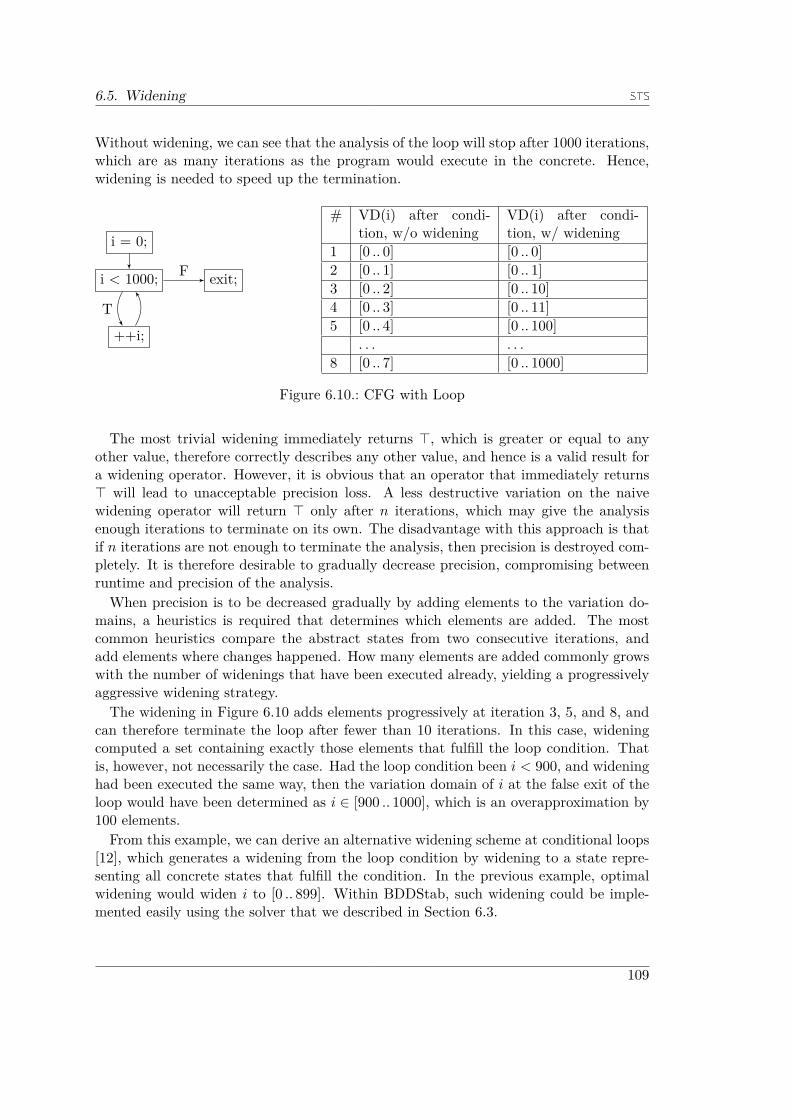
6.5. Widening

Without widening, we can see that the analysis of the loop will stop after 1000 iterations,which are as many iterations as the program would execute in the concrete. Hence,widening is needed to speed up the termination.

i = 0;

i < 1000;

++i;

exit;

T

F

# VD(i) after condi-tion, w/o widening

VD(i) after condi-tion, w/ widening

1 [0 .. 0] [0 .. 0]2 [0 .. 1] [0 .. 1]3 [0 .. 2] [0 .. 10]4 [0 .. 3] [0 .. 11]5 [0 .. 4] [0 .. 100]

. . . . . .8 [0 .. 7] [0 .. 1000]

Figure 6.10.: CFG with Loop

The most trivial widening immediately returns >, which is greater or equal to anyother value, therefore correctly describes any other value, and hence is a valid result fora widening operator. However, it is obvious that an operator that immediately returns> will lead to unacceptable precision loss. A less destructive variation on the naivewidening operator will return > only after n iterations, which may give the analysisenough iterations to terminate on its own. The disadvantage with this approach is thatif n iterations are not enough to terminate the analysis, then precision is destroyed com-pletely. It is therefore desirable to gradually decrease precision, compromising betweenruntime and precision of the analysis.When precision is to be decreased gradually by adding elements to the variation do-

mains, a heuristics is required that determines which elements are added. The mostcommon heuristics compare the abstract states from two consecutive iterations, andadd elements where changes happened. How many elements are added commonly growswith the number of widenings that have been executed already, yielding a progressivelyaggressive widening strategy.The widening in Figure 6.10 adds elements progressively at iteration 3, 5, and 8, and

can therefore terminate the loop after fewer than 10 iterations. In this case, wideningcomputed a set containing exactly those elements that fulfill the loop condition. Thatis, however, not necessarily the case. Had the loop condition been i < 900, and wideninghad been executed the same way, then the variation domain of i at the false exit of theloop would have been determined as i ∈ [900 .. 1000], which is an overapproximation by100 elements.From this example, we can derive an alternative widening scheme at conditional loops

[12], which generates a widening from the loop condition by widening to a state repre-senting all concrete states that fulfill the condition. In the previous example, optimalwidening would widen i to [0 .. 899]. Within BDDStab, such widening could be imple-mented easily using the solver that we described in Section 6.3.

109

6. BDDStab Jakstab Adapter

Instead, the widening strategy of the BDDStab adapter uses bisection to find changesbetween abstract states from two consecutive iterations. BDDs support bisection effi-ciently, as they support O(1) equivalence checking and their structure is derived from theShannon expansion, itself a form of applied bisection. The widening operator recursesinto the changed sub-BDDs to a depth determined by the number of previous widenings,and replaces the found sub-BDD by 1 , thereby adding more elements and reducing theBDD size at the same time.

The implementation of the widening operator of the BDDStab adapter was done aspart of a bachelor thesis, which contains a precise description of the operator [77].

6.6. CPA Configuration for BDDStab

After defining the transfer functions for Jakstab’s SSL, we are now ready to define a CPAinstance for BDDStab. As discussed previously, the CPA formulation that Jakstab usesallows the combination of analyses, facilitated by the required merge and join operators.By default, BDDStab uses the mergejoin and stopjoin operators, i.e., a configurationcorresponding to classic DFA. Additionally, Jakstab, by default, combines any analysiswith a location analysis, suitable for the analysis of executables. In this configuration,BDDStab constitutes a classic DFA, with the difference that the CFG is built within thelocation analysis and therefore is not static. Figure 6.11 contains the CPA instance forthe BDDStab adapter, where EBDD is the described composition of an abstract variabletable and a heap model, both using BDD-based integer sets for abstract values. Asusual, each abstract BDD state is paired with an abstract location, which we treat asequivalent to the disassembled instruction at this position. The transfer relation BDDis defined between combinations of location and BDD state, exactly when the right-hand side location is reachable from the left-hand side, and the transfer function of theBDDStab adapter maps the left-hand BDD state to the right-hand side BDD state. Themerge operator merges only states with identical locations and the stop operator is trueexactly when the join of all states for a location covers the new state. Note that as before,we do not provide the domain of concrete states C and the concretization function J·K,as they are not needed for the execution of the analysis. Furthermore, we assume thelocation analysis as implemented in Jakstab, i.e., we assume that it implicitly uses ourabstract evaluation function to resolve jump targets.

110

6.6. CPA Configuration for BDDStab

EBDD = (EL × EBDDSet)

(l1, σ#BDD1 ) BDD (l2, σ#BDD

2 ) ⇐⇒ l1 L l2 ∧ fBDDl1 (fEQ

l1(σ#BDD

1 )) = σ#BDD2

mergeBDD((l1, σ#BDD1 ), (l2, σ#BDD

2 )) ={

(l1,mergejoin(σ#BDD1 , σ#BDD

2 )) if l1 = l2

(l2, σ#BDD2 ) otherwise

stopBDD((l1, σ#BDD), R) = stopjoin(σ#BDD, {σ#BDD2 | (l2, σ#BDD

2 ) ∈ R, l2 = l1})

DBDD = ((C, EBDD, J·K), BDD,mergeBDD, stopBDD)

ιBDD = (l, ∅) where l is an entry node of the analyzed program

Figure 6.11.: BDDStab CPA

111

6. BDDStab Jakstab Adapter

6.7. Implementation of BDDStab Jakstab AdapterThe implementation of the Jakstab adapter consists of 6 Java classes. The main entrypoint to the analysis is the BDDTracking class that contains the CPA instance. ThisCPA instance uses abstract environments, implemented in the BDDState class, whichcontains the transfer function and abstract evaluation functions, and therefore containsthe adapter’s main functionality. The BDDSet class, which implements abstract values,wraps a BDD-based integer set from the BDDStab library, and re-exports most of itsfunctionality. Since Jakstab’s output contains string representations of abstract values,the BDDSet class must provide a pretty printer. However, since abstract values inBDDStab are capable of representing many concrete elements, and the output as BDDis not helpful, we only explicitly show sets with up to 100 elements. Should the setcontain more elements, then its cardinality is displayed instead.

UsageThe analysis is activated using “z” as a parameter to Jakstab’s “–cpa” option. Toactivate the restriction of flow data at conditional branches (Assume statement), theanalysis must be combined with Jakstab’s forward substitution analysis, which is doneby additionally passing “f” to “–cpa”. The analysis additionally supports a thresholdparameter (“–bdd-threshold”), that determines when widening should take place, and aconcretization threshold (“–bdd-concthreshold”) that defines up to how many elementsconcretizations may take place. The concretization threshold is important, as it deter-mines up to how many addresses may be considered during a write to the heap, and upto how many targets may be considered when resolving jumps.To analyze the binary “demo.exe” using BDDStab, one could call Jakstab as follows:

./jakstab -m demo.exe --cpa fz --bdd-threshold 3 --bdd-concthreshold 1000

112

6.8. Evaluation

6.8. Evaluation

Because of the unique challenges connected to sound CFR on binaries, it is unlikelythat integer value analysis, even if precise, is enough to produce sound CFGs for largerreal-world programs. With this evaluation, we provide an insight into the performanceof our domain when applied to real-world programs. Hence, we chose the CPU2006[78] as benchmark suite, which contains such programs. For the evaluation, we use aconfiguration of Jakstab that makes the least number of assumptions about the analyzedprograms. Specifically, no assumptions about the stack discipline of included functionsare made.

6.8.1. The CPU2006 Benchmark Suite

The CPU2006 benchmark suite was designed to measure the performance of compilers aswell as the integer and floating point performance of computers and is now widely usedfor this purpose [79]. The suite contains 17 floating point benchmarks and 13 integerbenchmarks from various domains, including fluid dynamics, biochemistry, linear pro-gramming, video compression, and path finding algorithms. The benchmark programsare written in C, C++, and Fortran, and perform an expensive calculation dependingon input that is included in the benchmark suite.We chose the CPU benchmark suite because it is well-known [79] and contains adap-

tations of real-world programs each of which compiles to a single executable. Theseexecutables do not load code at runtime, which would complicate the analysis withJakstab.However, the benchmark was not designed for benchmarking binary analyzers. More

than half of the programs perform mostly floating point operations, which are notsupported by our domain. Consequently, these operations are interpreted as non-deterministic in the analysis. Furthermore, the programs perform computations de-pending on input that the CPU2006 suite provides. It is unclear whether the programsassume correctly formatted input and exhibit undefined runtime behavior if presentedwith invalid input. If so, then it is possible that the programs contain unbounded controlflow and the analysis using a sound analyzer will fail because not all jump targets canbe resolved.

6.8.2. Measuring Procedure

The benchmarks are compiled using GCC version 4.8.4, provided by Ubuntu 14.04.3.We use the flag “no-stack-protector” as well was the option “-m32” to suppress stackprotection and generate 32-bit code, as Jakstab lacks support for the 64-bit instructionset. Furthermore, we create and measure each binary for the optimization levels 0 to 3,and s. For the measuring procedure, we apply Jakstab with the options “–cpa fz”, “–bdd-threshold 10”, and “–bdd-concthreshold 1000”, i.e., we activate forward substitution andBDDStab, use widening after 10 iterations and concretize sets with up to 1000 elements.This configuration means that Jakstab will use its pessimistic resolve operator, which

113

6. BDDStab Jakstab Adapter

means that if a dynamic jump cannot be resolved by BDDStab, then the analysis isstopped. We use the pessimistic resolve operator as it makes no assumptions about theexecutable and is therefore sound for any executable. If the analysis took more than 10hours, we terminated it. After termination of Jakstab, we parse its output to generateour measurements. If the analysis was terminated prematurely, and this has lead tospecific measurements to not be made, then we denote this in our data using the ⊥symbol.

6.8.3. Data Description

In this section, we describe the individual columns of our CPU2006 evaluation data.

Opt The optimization level passed to GCC during for compilation. O0 means no opti-mization, whereas O3 means maximum optimization. O1 and O2 enable optimizationsthat should not incur any speed-space tradeoffs, such as loop unrolling, which may in-crease the executable’s size. In difference to O1, O2 includes expensive optimizationssuch as instruction scheduling, which is a technique to improve pipeline efficiency. O3enables optimizations that try to improve execution speed but may increase the gen-erated executable such as inlining of functions. Os instructs the compiler to generatesmall executables, e.g., to run on size constrained systems such as microcontrollers.

Program The name of the analyzed program from the CPU 2006 benchmark suite.

Instrs The number of disassembled assembly instructions. This measurement gives aninsight into the size of executables that we can expect Jakstab with BDDStab to analyzesoundly.

IL Instrs The number of analyzed intermediate language instructions. During analysis,each disassembled assembly instruction gets lifted to Jakstab’s intermediate language.Since each instruction at assembly level may produce several instructions at the level ofthe intermediate language, the number of intermediate language instructions is generallygreater than that on assembly level. This measurement gives an insight into how manyIL instructions on average are needed to represent assembly instructions, and how manyour analysis actually analyzed.

IBran The number of disassembled indirect branches at assembly level. A branchinstruction in X86 is considered indirect if its target is not described by a constant offsetto the program counter or by a constant. Furthermore, the target may not lie in thestatic data region of the binary.

UBran The number of unresolved targets on intermediate language level. A target ofa jump instruction in the intermediate language is considered unresolved, if the analysiscould not produce a set of target addresses. Within BDDStab, if the variation domain

114

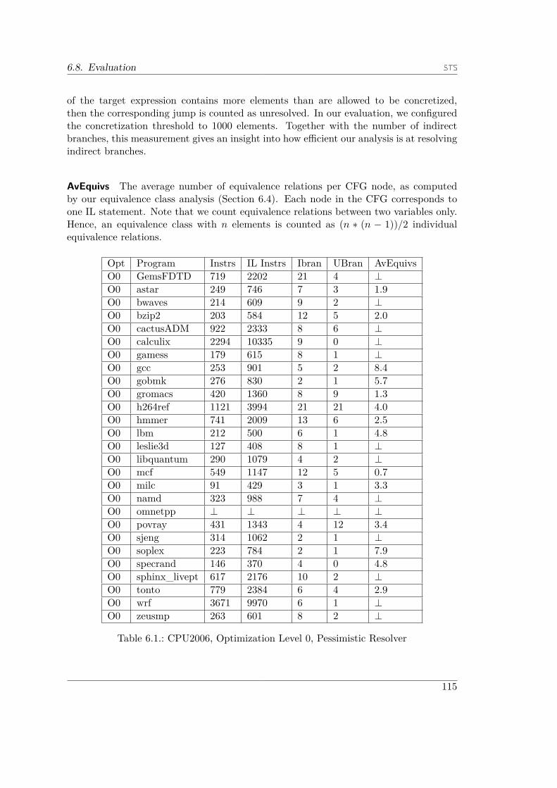
6.8. Evaluation

of the target expression contains more elements than are allowed to be concretized,then the corresponding jump is counted as unresolved. In our evaluation, we configuredthe concretization threshold to 1000 elements. Together with the number of indirectbranches, this measurement gives an insight into how efficient our analysis is at resolvingindirect branches.

AvEquivs The average number of equivalence relations per CFG node, as computedby our equivalence class analysis (Section 6.4). Each node in the CFG corresponds toone IL statement. Note that we count equivalence relations between two variables only.Hence, an equivalence class with n elements is counted as (n ∗ (n − 1))/2 individualequivalence relations.

Opt Program Instrs IL Instrs Ibran UBran AvEquivsO0 GemsFDTD 719 2202 21 4 ⊥O0 astar 249 746 7 3 1.9O0 bwaves 214 609 9 2 ⊥O0 bzip2 203 584 12 5 2.0O0 cactusADM 922 2333 8 6 ⊥O0 calculix 2294 10335 9 0 ⊥O0 gamess 179 615 8 1 ⊥O0 gcc 253 901 5 2 8.4O0 gobmk 276 830 2 1 5.7O0 gromacs 420 1360 8 9 1.3O0 h264ref 1121 3994 21 21 4.0O0 hmmer 741 2009 13 6 2.5O0 lbm 212 500 6 1 4.8O0 leslie3d 127 408 8 1 ⊥O0 libquantum 290 1079 4 2 ⊥O0 mcf 549 1147 12 5 0.7O0 milc 91 429 3 1 3.3O0 namd 323 988 7 4 ⊥O0 omnetpp ⊥ ⊥ ⊥ ⊥ ⊥O0 povray 431 1343 4 12 3.4O0 sjeng 314 1062 2 1 ⊥O0 soplex 223 784 2 1 7.9O0 specrand 146 370 4 0 4.8O0 sphinx_livept 617 2176 10 2 ⊥O0 tonto 779 2384 6 4 2.9O0 wrf 3671 9970 6 1 ⊥O0 zeusmp 263 601 8 2 ⊥

Table 6.1.: CPU2006, Optimization Level 0, Pessimistic Resolver

115

6. BDDStab Jakstab Adapter

6.8.4. Results

Tables 6.1, 6.2, 6.3, 6.4, and 6.5 show the results of applying Jakstab with BDDStab onthe CPU2006 programs, compiled with varying optimization levels. These tables do notlist results for the “dealII”, “perlbench”, and “xalancbmk” benchmarks, as Jakstab waseither not able to parse the corresponding ELF file, or BDDStab was not able to provideany usable result in time. The tables use the ⊥ symbol, if no result could be obtainedfor the corresponding measurement. Since the AvEquivs measurement depends on thenumber of CFG edges on IL level, it requires a CFG to be generated, which does nothappen if the analysis terminated abnormally.

Opt Program Instrs IL Instrs Ibran UBran AvEquivsO1 GemsFDTD 368 1021 20 5 ⊥O1 astar 294 981 9 4 1.2O1 bwaves 849 3523 9 0 ⊥O1 bzip2 100 351 4 2 3.7O1 cactusADM 752 2230 5 7 4.7O1 calculix 40 484 1 0 3.9O1 gamess 1971 8116 10 0 ⊥O1 gcc 71 595 2 1 7.4O1 gobmk 217 767 2 1 5.0O1 gromacs 262 1047 7 4 2.9O1 h264ref 326 922 14 7 1.7O1 hmmer 325 1049 5 6 4.9O1 lbm 166 414 6 1 6.8O1 leslie3d 783 3655 8 2 ⊥O1 libquantum ⊥ ⊥ ⊥ ⊥ ⊥O1 mcf 499 1168 12 8 ⊥O1 milc 76 410 3 1 3.4O1 namd 86 370 5 2 2.9O1 omnetpp ⊥ ⊥ ⊥ ⊥ ⊥O1 povray 236 1045 3 7 2.6O1 sjeng 146 573 2 1 3.5O1 soplex 236 980 3 0 ⊥O1 specrand 124 313 4 0 3.2O1 sphinx_livept 236 833 8 5 ⊥O1 tonto 513 1636 5 3 3.5O1 wrf 1445 3821 4 1 ⊥O1 zeusmp 231 545 8 2 2.1

Table 6.2.: CPU2006, Optimization Level 1, Pessimistic Resolver

With BDDStab resolving dynamic jumps, Jakstab was able to disassemble between

116

6.8. Evaluation

40 (“calculix”, O1) and 18070 (“wrf”, O3) instructions. Since the “wrf” executable is4.3 megabytes in size, it is safe to assume that even in the optimal case, our analysisonly covered a small part of the executable before it stopped. Overall, each assemblyinstruction gets translated to about 3 instructions in Jakstab’s intermediate language.

Opt Program Instrs IL Instrs Ibran UBran AvEquivsO2 GemsFDTD 2325 9673 22 10 ⊥O2 astar 308 1075 9 3 2.0O2 bwaves 580 2269 9 1 ⊥O2 bzip2 102 360 4 2 3.4O2 cactusADM 679 2101 6 1 ⊥O2 calculix 44 497 1 0 3.8O2 gamess 209 745 7 0 ⊥O2 gcc 66 583 3 1 8.7O2 gobmk 217 783 2 1 4.9O2 gromacs 732 2874 12 8 ⊥O2 h264ref 325 962 14 7 ⊥O2 hmmer 298 1038 5 6 4.1O2 lbm 171 431 6 1 5.6O2 leslie3d 779 3571 9 1 ⊥O2 libquantum 239 677 6 2 1.5O2 mcf 483 1123 12 8 ⊥O2 milc 78 422 3 1 3.3O2 namd 82 364 5 2 2.8O2 omnetpp 346 1397 16 9 0.9O2 povray 225 1041 3 7 2.5O2 sjeng 147 598 2 1 3.3O2 soplex 170 798 3 0 ⊥O2 specrand 124 335 4 0 3.9O2 sphinx_livept 585 2185 9 4 ⊥O2 tonto 527 1642 5 3 3.2O2 wrf 1421 3697 4 1 ⊥O2 zeusmp 242 559 8 2 1.9

Table 6.3.: CPU2006, Optimization Level 2, Pessimistic Resolver

It may be surprising that the “UBran” column can contain greater numbers than the“IBran” column. Unfortunately, the number of successfully resolved indirect branchescannot be computed by subtracting the “UBran” column from the “IBran” column,because the “IBran” column refers to instructions on assembly level, while the “UBran”column refers to instructions on the IL level. Furthermore, “UBran” lists all instanceswhere the analysis was unable to determine a set of successors. Therefore, “UBran”includes cases where the analysis was unable to resolve return statements, which can

117

6. BDDStab Jakstab Adapter

happen if the precision of the stack has deteriorated. An example of such a case isthe “povray” benchmark in optimization level O1. Therefore, the number of resolvedindirect branches can be larger than the difference between the “UBran” and “IBran”columns, suggesting that BDDStab is effective at resolving dynamic jumps, but must beimproved in terms of context sensitivity.

Opt Program Instrs IL Instrs Ibran UBran AvEquivsO3 GemsFDTD 1322 5249 21 7 ⊥O3 astar 287 967 9 3 0.7O3 bwaves 567 2229 9 0 ⊥O3 bzip2 103 367 4 2 3.4O3 cactusADM 527 1595 6 1 ⊥O3 calculix 44 497 1 0 3.8O3 gamess 242 853 7 0 ⊥O3 gcc 66 583 3 1 8.0O3 gobmk 211 772 2 1 4.5O3 gromacs 700 2713 12 8 ⊥O3 h264ref ⊥ ⊥ ⊥ ⊥ ⊥O3 hmmer 298 1038 5 6 4.2O3 lbm 171 431 6 1 5.6O3 leslie3d ⊥ ⊥ ⊥ ⊥ ⊥O3 libquantum 239 672 6 2 1.6O3 mcf ⊥ ⊥ ⊥ ⊥ ⊥O3 milc 79 430 3 1 3.3O3 namd 82 364 5 2 2.8O3 omnetpp 346 1397 16 9 0.9O3 povray 212 1019 3 3 3.0O3 sjeng 147 598 2 1 3.2O3 soplex 196 845 3 0 ⊥O3 specrand 124 330 4 0 3.6O3 sphinx_livept 819 3152 10 4 ⊥O3 tonto 507 1586 5 2 3.1O3 wrf 18070 80923 6 1 ⊥O3 zeusmp 242 577 8 2 1.9

Table 6.4.: CPU2006, Optimization Level 3, Pessimistic Resolver

The “AvEquivs” column shows that there exist up to 8.7 equivalence relations onaverage per CFG node (“gcc”, O2). However, in this benchmark, the analysis onlyrecovered 66 instructions. The fewer instructions are analyzed, the more likely is thenumber of equivalence relations per node overestimated, because when more parts ofthe CFG are reconstructed, back edges may lead to additional confluence points. Thejoin of the equivalence class analysis only keeps two variables in the same equivalence

118

6.8. Evaluation

class if they are considered equivalent in all incoming flow data. We therefore believethe 1.5 equivalence relations per CFG node in the “povray” benchmark for optimizationlevel Os to be more realistic. The high number of equivalences for programs with fewerrecovered instructions is still potentially contributing to the analysis’ precision duringanalysis.

Opt Program Instrs IL Instrs Ibran UBran AvEquivsOs GemsFDTD 108 523 7 1 3.2Os astar 369 1122 8 3 2.4Os bwaves ⊥ ⊥ ⊥ ⊥ ⊥Os bzip2 97 379 4 1 3.7Os cactusADM 1213 4049 7 1 ⊥Os calculix 54 514 1 0 4.0Os gamess ⊥ ⊥ ⊥ ⊥ ⊥Os gcc 85 633 2 1 8.4Os gobmk 467 1276 1 3 1.6Os gromacs 318 1231 7 5 2.1Os h264ref 414 1363 15 17 2.0Os hmmer 131 690 3 2 5.7Os lbm 186 535 6 1 6.8Os leslie3d 292 1187 8 0 ⊥Os libquantum 166 588 4 1 2.3Os mcf ⊥ ⊥ ⊥ ⊥ ⊥Os milc 99 472 3 1 4.2Os namd 259 704 8 3 1.0Os omnetpp ⊥ ⊥ ⊥ ⊥ ⊥Os povray 3176 10430 3 9 1.5Os sjeng 151 605 2 1 3.7Os soplex 107 558 2 1 4.8Os specrand 130 383 4 0 4.5Os sphinx_livept 857 3296 11 15 ⊥Os tonto 353 1244 5 3 4.3Os wrf 189 965 4 1 2.2Os zeusmp 158 490 8 0 ⊥

Table 6.5.: CPU2006, Optimization Level s, Pessimistic Resolver

119

7. Future Work

In this chapter, we discuss future research directions to improve the efficiency and pre-cision of our BDD-based, non-convex abstract domain.

Benchmark SuiteAs described in the evaluation of our Jakstab plug-in, one cannot yet hope to performsound binary analysis of real-world programs such as those in the CPU2006 benchmarksuite, which is not surprising as this benchmark suite was not designed for benchmarkingbinary analyzers. Simply compiling benchmark suites for software analyzers on struc-tured languages is insufficient to produce a useful benchmark suite for binary analyzers,since the challenges in these suites are often to detect undefined runtime behavior such asout of bounds array access. As discussed briefly in Section 2.1, the compiler may producecode with unbounded control flow, i.e., a jump instruction with non-deterministic target,for source code with undefined behavior. Binary analyzers cannot decide whether thesource of such a non-deterministic jump is undefined behavior in the source program, oroverapproximation during the analysis. A specialized benchmark suite for sound binaryanalyzers would contain for each instruction of an executable in the suite a trace thatproves that this instruction is indeed reachable. This information can then be used asground truth during the evaluation of an analyzer.

Tree-based Heap ModelOur domain is efficient at working with large VDs. However, in the BDDStab adapter,there are two operations that force concretization, which is not feasible for large VDs:

1. Heap Access

2. Resolve Operator

The resolve operator is used by Jakstab to compute successor abstract locations froman abstract state and an instruction. Heap access forces concretization, because we usethe heap model of Jakstab, which is based on a simple map structure from heap addressesto abstract values. Therefore, when reading and writing to a heap address represented bya VD with n elements, n map accesses are performed, which may be unacceptable. Anabstract heap based on binary tree structures similar to multi-terminal BDDs (MTBDD)[66], could be used to speed up read and write operations, if the BDD representationof the address VD is efficient. We envision this binary tree structure to have the sameinterpretation of its edges as our BDD-based integer sets, i.e., the edges correspond tothe bits in the heap address. As in our BDD structure, sub-trees would correspondto an interval of heap addresses. All nodes in the heap tree would contain a BDDthat represents all abstract values written to exactly this interval of heap addresses.

121

7. Future Work

Therefore, performing a weak update would traverse the address BDD and the heaptree together until a 1 is found in the address BDD. Then, the BDD stored in thecorresponding heap tree node is updated to the union of the abstract value that must bestored and previously stored value. Read operations would again traverse the addressBDD and the heap tree together, while unioning all BDDs in the heap tree’s nodes. Ifa 1 node is found in the address BDD, then the complete sub-heap-tree must still betraversed to collect also those values written to sub-address ranges. However, it shouldbe possible to cache in each heap tree node the union of all BDDs in the nodes on thepath to this node, as well as the union of all BDDs below this node. This caching mustbe implemented lazily to avoid traversing the whole heap tree in each operation.

Context Sensitivity

The current CPA configuration for our domain is equivalent to classic DFA. Therefore,we currently join the incoming data flow information at each confluence point. In thisjoin, the stack of all abstract states get merged. Because the stack contains the returnaddresses from function calls, joining the stack destroys context sensitivity. Jakstabcontains a CPA that uses call strings [80] to avoid joining different contexts. Yet, usingthis domain is only sound if the analyzed program uses stack discipline, i.e., does notchange the return address explicitly. By changing the CPA merge operator to merge onlyabstract states with equal stack value, or merging only if there are too many abstractstates with the same abstract location, limited context sensitivity could be achievedwithout assuming stack discipline.

Naive Sets for Small VDs

Our BDD-based domain remains efficient for large integer sets. However, for small sets,it is likely that our transfer functions are slower than those on naive sets. It is thereforepossible to speed up our domain using naive sets for VDs with fewer elements thana given threshold and BDD-based integer sets otherwise. To avoid creating naive setsthat are larger than the threshold, transfer functions on naive sets must be able toapproximate the size of their result. Using a non-relational abstraction, as we do inour domain, the size of the result of most transfer functions can safely be approximatedusing the multiplication of all operand set sizes. Should this multiplication be above thethreshold, then BDD-based sets are used in the computation.

Relational Information in Transfer Functions

By itself, our integer value analysis domain is non-relational, which compromises preci-sion for efficiency. However, we believe that introducing relational information can beused to improve the precision as well as the efficiency of our transfer functions. The com-putation of this relational information would be left to an extra domain, e.g., the equiv-

122

alence class domain presented in Section 6.4. The exact abstract version of the binaryoperator ◦ of non-relational value analysis domains computes {a ◦ b | a ∈ A, b ∈ B}, i.e.,it combines every value from the VD A with every value form the VD B. If it is knownthat the variables whose values these VDs represent must have equal value at runtime,then the result of the transfer function can be simplified to {a◦b | a ∈ A, b ∈ B, a == b},which is likely to contain fewer elements, corresponding to better precision, but is alsopotentially easier to compute because fewer combinations must be considered.Generally, our algorithms for binary transfer functions use four recursive calls in the

case where both BDDs are non-terminals. These four recursive calls use all four combi-nations of the two decision node’s sub-BDDs as arguments. With the equality constraint,the number of recursive calls can be reduced to two, namely those on both true successorBDDs and both false successor BDDs, as equal integers have the same bit pattern andthe edges encode the bits.It is also possible to support more complex constraints such as ±a ± b ≤ c, where c

is a constant, as computed by the octagon abstract domain [15]. A path of length mto a decision node in the BDD of an unsigned n-bit integer set, described by an m-bitbitvector p, corresponds to a weight of pv = ∑m−1

i=0 p{i} ∗ 2i+n−m−1 in the integers thatinclude the bitvector as their first m bits. Hence, all these integers are greater or equalthan pv and smaller or equal than pv + 2n−m − 1. Our algorithms can use these boundsto decide whether the BDDs of a recursive call can fulfill the constraint or not. If theBDDs cannot fulfill the constraint, then the recursive call does not have to be executed.

123

8. Conclusion

In this dissertation, we presented an abstract domain for integer value analysis. We makethe implementation of this abstract domain available in the BDDStab library, and useit to implement an integer value analysis for binaries using the Jakstab binary analysisframework. The domain uses BDD-based integer sets to implement efficient abstractvalues that neither enforce convexity nor are restricted to a specific type of non-convexity.Hence, this domain does not suffer from any precision loss through joining at confluencepoints, other than the loss that is caused by its non-relational abstraction. To supportBDD-based integer sets, we define a variation of classic BDDs with complement edgesthat differs in two ways:

1. Labelless Decision Nodes

2. Precomputed Satisfiability Counts

Labelless decision nodes allow the sharing of structurally equivalent BDDs that havedifferent semantics. This extension compromises on the efficiency of BDD reduction, aseach decision node’s label is given by the length of the path from the BDD’s root node toit. Since our BDDs only contain path lengths of up to the bitwidths of the representedintegers, which are usually 64, this compromise seems advantageous, especially becauseimproved sharing also improves the memoization of algorithms.Precomputed satisfiability counts allow us to determine in O(1) the number of different

paths from a BDD’s root node to a true terminal. In our BDD-based integer sets,satisfiability count corresponds to the set cardinality.We define algorithms for the most common transfer functions that are defined on the

structure of the BDDs instead of the integers they represent. Hence our algorithms areefficient even on very large integer sets. The algorithms for bitwise and and or, as well asthe algorithms for addition and subtraction, are exact in the non-relational case. Otheralgorithms such as multiplication, shifts, and rotations are only exact when one operandset is a singleton, as exact versions that do not rely on concretization are not known.Efficient conversion from strided intervals and to regular intervals allows us to fall backon known transfer functions when no more precise algorithm is known.Our BDDStab adapter plug-in for the binary analysis framework Jakstab implements

BDD-based value analysis for binaries. The reliance of machine code on dynamicallycomputed jumps, necessitates precise analysis of jump target addresses. Since the dis-tribution of target addresses within an executable is arbitrary, arbitrary sets are neededfor a precise representation of the abstract target value.The treatment of conditional jumps in the analysis of executables is challenging, be-

cause the jump condition does not directly depend on registers or memory locations,but instead on formulas over special variables called flags, the value of which in turndepends on registers and memory locations. Since a non-relational abstraction losesthe relationship between registers, memory locations, and flags, non-relational analyz-ers can only compute restrictions for flags at conditional jumps, and not for registers

125

8. Conclusion

and memory locations as required. We use a combination of forward substitution andsimplification to translate conditions back to registers and memory locations, and thenuse our overapproximating constraint solver for BDD-based integer sets to create anabstract state that represents all states that fulfill the constraint. To restrict not onlythose abstract values of registers and memory locations that are directly referenced inthe simplified constraint, but also those that must have equal values at runtime, we de-fine and implement a specialized analysis that computes equivalence relations betweenstorage locations.In difference to most other abstractions used in integer value analyses, such as strided

intervals, our BDD-based integer sets require no approximation. However, as the evalu-ation of our BDDStab library shows, they can still efficiently exploit regularities in therepresented sets. The performance evaluation of our BDD-based integer sets for inter-vals and congruence classes leads us to expect that our sets are efficient at representingset shapes that are similar to the evaluated ones. For example, if a strided interval isjoined with a singleton interval that is not in the strided interval’s congruence class, thenthe resulting join will have a stride of 1. Our BDD-based integer sets simply add thissingleton without approximation.The evaluation of the BDDStab library also shows that the performance of the eval-

uated algorithms does not depend on the size of the operand sets, but rather on thestructure of the associated BDDs, which allows our algorithms to remain efficient evenfor large integer sets. The evaluation using congruence classes, which contain many ref-erences to the same sub-BDD in memory, showed that our algorithms avoid recomputingresults for previously computed operands.The evaluation of our BDDStab adapter using CPU2006 benchmarks confirms that

it is necessary for a binary analysis framework to resolve indirect branches, and thatour integer value analysis is able to do so. Furthermore, the evaluation substantiatesour assumption that equivalence relations between storage locations are frequent in themachine code representation of programs. This discovery justifies our implementationof a dedicated equivalence analysis.The low number of analyzed instructions in the CPU2006 benchmark shows that,

without further assumptions about the binary, sound analysis of real-world executablesis not yet within the capabilities of integer value analysis, even if it focuses on precisionas BDDStab does. Smaller sized programs, such as the example from Section 2.1, canbe analyzed soundly using a combination of Jakstab and BDDStab, which suggests thatBDDStab will be useful in the analysis of parts of executables, e.g., functions. Hence, wesuggest further research in combining BDDStab with unsound analysis methods, suchas identifying functions in binaries, or iteratively improving precision only if needed.The unique challenges of the analysis of binaries cannot be solved using only well-

known techniques from the analysis of structured programs. We think that the combi-nation of precise value analyzers with heuristics that guide the analysis is the directionthat future research should take.

126

Bibliography

Bibliography

[1] S. Mattsen, A. Wichmann, and S. Schupp, “BDDStab: BDD-based Value Analy-sis of Binaries,” in The Fifth Workshop on Tools for Automatic Program Analysis(TAPAS), 2014.

[2] S. Mattsen, A. Wichmann, and S. Schupp, “A non-convex abstract domain for thevalue analysis of binaries,” in 2015 IEEE 22nd International Conference on SoftwareAnalysis, Evolution, and Reengineering (SANER), pp. 271–280, Mar. 2015.

[3] J. Kinder and H. Veith, “Jakstab: A Static Analysis Platform for Binaries,” in Com-puter Aided Verification (A. Gupta and S. Malik, eds.), Lecture Notes in ComputerScience, pp. 423–427, Springer, July 2008.

[4] O. J. Dahl, E. W. Dijkstra, and C. A. R. Hoare, eds., Structured Programming.London, UK, UK: Academic Press Ltd., 1972.

[5] A. M. Turing, “On Computable Numbers, with an Application to the Entschei-dungsproblem,” Proceedings of the London Mathematical Society, vol. 42, pp. 230–265, Jan. 1937.

[6] X. Meng and B. P. Miller, “Binary Code is Not Easy,” in Proceedings of the 25thInternational Symposium on Software Testing and Analysis, ISSTA 2016, (NewYork, NY, USA), pp. 24–35, ACM, 2016.

[7] T. Bao, J. Burket, M. Woo, R. Turner, and D. Brumley, “BYTEWEIGHT: Learn-ing to Recognize Functions in Binary Code,” in Proceedings of the 23rd USENIXConference on Security Symposium, SEC’14, (Berkeley, CA, USA), pp. 845–860,USENIX Association, 2014.

[8] B. Schwarz, S. Debray, and G. Andrews, “Disassembly of Executable Code Revis-ited,” in Proceedings of the 9th Working Conference on Reverse Engineering, WCRE’02, (Washington, DC, USA), pp. 45–54, IEEE Computer Society, 2002.

[9] “Radare: a Portable Reversing Framework.” www.radare.org. Last accessed 29March 2017.

[10] “IDAPro: The Interactive Disassembler.” www.hex-rays.com/products/ida. Lastaccessed 29 March 2017.

[11] C. Linn and S. Debray, “Obfuscation of Executable Code to Improve Resistance toStatic Disassembly,” in Proceedings of the 10th ACM Conference on Computer andCommunications Security, CCS ’03, (New York, NY, USA), pp. 290–299, ACM,2003.

[12] A. Sepp, B. Mihaila, and A. Simon, “Precise Static Analysis of Binaries by Ex-tracting Relational Information,” in Proceedings of the 18th Working Conference

127

Bibliography

on Reverse Engineering, WCRE ’11, (Washington, DC, USA), pp. 357–366, IEEEComputer Society, 2011.

[13] H. G. Rice, “Classes of Recursively Enumerable Sets and Their Decision Problems,”Transactions of the American Mathematical Society, vol. 74, no. 2, pp. 358–366,1953.

[14] T. Ball and S. K. Rajamani, “The SLAM Toolkit,” in Computer Aided Verification,Lecture Notes in Computer Science, (London, UK), pp. 260–264, Springer, 2001.

[15] A. Miné, “The Octagon Abstract Domain,” Higher Order Symbolic Computation,vol. 19, pp. 31–100, Mar. 2006.

[16] J. Kinder and H. Veith, “Precise Static Analysis of Untrusted Driver Binaries,” inProceedings of the 2010 Conference on Formal Methods in Computer-Aided Design,FMCAD ’10, (Austin, TX), pp. 43–50, FMCAD Inc, 2010.

[17] B. Blanchet, P. Cousot, R. Cousot, J. Feret, L. Mauborgne, A. Miné, D. Monniaux,and X. Rival, “A Static Analyzer for Large Safety-critical Software,” in Proceedingsof the ACM SIGPLAN 2003 Conference on Programming Language Design andImplementation, PLDI ’03, (New York, NY, USA), pp. 196–207, ACM, 2003.

[18] P. Cuoq, J. Signoles, P. Baudin, R. Bonichon, G. Canet, L. Correnson, B. Monate,V. Prevosto, and A. Puccetti, “Experience Report: OCaml for an Industrial-strength Static Analysis Framework,” in Proceedings of the 14th ACM SIGPLANInternational Conference on Functional Programming, ICFP ’09, (New York, NY,USA), pp. 281–286, ACM, 2009.

[19] P. Cousot and R. Cousot, “Static determination of dynamic properties of programs,”in Proceedings of the Second International Symposium on Programming, pp. 106–130, Dunod, Paris, France, 1976.

[20] P. Cousot and N. Halbwachs, “Automatic Discovery of Linear Restraints AmongVariables of a Program,” in Proceedings of the 5th ACM SIGACT-SIGPLAN Sympo-sium on Principles of Programming Languages, POPL ’78, (New York, NY, USA),pp. 84–96, ACM, 1978.

[21] L. Chen, A. Miné, and P. Cousot, “A Sound Floating-Point Polyhedra AbstractDomain,” in Programming Languages and Systems (G. Ramalingam, ed.), LectureNotes in Computer Science, pp. 3–18, Springer, Dec. 2008.

[22] K. Ghorbal, E. Goubault, and S. Putot, “The Zonotope Abstract Domain Tay-lor1+,” in Computer Aided Verification (A. Bouajjani and O. Maler, eds.), LectureNotes in Computer Science, pp. 627–633, Springer, June 2009.

[23] G. Balakrishnan and T. Reps, “WYSINWYX: What You See is Not What YoueXecute,” ACM Transactions on Programming Languages and Systems, vol. 32,pp. 23:1–23:84, Aug. 2010.

128

Bibliography

[24] J. Brauer, A. King, and S. Kowalewski, “Abstract Interpretation of MicrocontrollerCode: Intervals Meet Congruences,” Science of Computer Programming, vol. 78,pp. 862–883, July 2013.

[25] P. Granger, “Static Analysis of Linear Congruence Equalities Among Variables ofa Program,” in Proceedings of the International Joint Conference on Theory andPractice of Software Development on Colloquium on Trees in Algebra and Program-ming (CAAP ’91): Vol 1, TAPSOFT ’91, (New York, NY, USA), pp. 169–192,Springer, 1991.

[26] E. M. Clarke and E. A. Emerson, “Design and Synthesis of Synchronization Skele-tons Using Branching-Time Temporal Logic,” in Logic of Programs, Workshop,(London, UK, UK), pp. 52–71, Springer, 1982.

[27] K. L. McMillan, Symbolic Model Checking. Norwell, MA, USA: Kluwer AcademicPublishers, 1993.

[28] D. Beyer, T. A. Henzinger, and G. Théoduloz, “Configurable Software Verification:Concretizing the Convergence of Model Checking and Program Analysis,” in Com-puter Aided Verification (W. Damm and H. Hermanns, eds.), no. 4590 in LectureNotes in Computer Science, pp. 504–518, Springer, July 2007.

[29] S. Mattsen, P. Cuoq, and S. Schupp, “Driving a sound static software analyzerwith branch-and-bound,” in 2013 IEEE 13th International Working Conference onSource Code Analysis and Manipulation (SCAM), pp. 63–68, Sept. 2013.

[30] K. Ghorbal, F. Ivančić, G. Balakrishnan, N. Maeda, and A. Gupta, “Donut Do-mains: Efficient Non-convex Domains for Abstract Interpretation,” in Proceedingsof the 13th International Conference on Verification, Model Checking, and AbstractInterpretation, VMCAI’12, (Berlin, Heidelberg), pp. 235–250, Springer, 2012.

[31] L. Chen, J. Liu, A. Miné, D. Kapur, and J. Wang, “An Abstract Domain to In-fer Octagonal Constraints with Absolute Value,” in Static Analysis Symposium(M. Müller-Olm and H. Seidl, eds.), Lecture Notes in Computer Science, pp. 101–117, Springer, Sept. 2014.

[32] G. A. Kildall, “A Unified Approach to Global Program Optimization,” in Proceed-ings of the 1th ACM SIGPLAN-SIGACT Symposium on Principles of ProgrammingLanguages, POPL ’73, (New York, NY, USA), pp. 194–206, ACM, 1973.

[33] C. Lattner, LLVM: An Infrastructure for Multi-Stage Optimization. PhD thesis,Computer Science Dept., University of Illinois at Urbana-Champaign, Urbana, IL,Dec. 2002.

[34] U. P. Khedker and D. M. Dhamdhere, “Bidirectional Data Flow Analysis: Mythsand Reality,” SIGPLAN Not., vol. 34, pp. 47–57, June 1999.

129

Bibliography

[35] M. Madsen and A. Møller, “Sparse Dataflow Analysis with Pointers and Reach-ability,” in Static Analysis (M. Müller-Olm and H. Seidl, eds.), Lecture Notes inComputer Science, pp. 201–218, Springer, Sept. 2014.

[36] P. Cousot and R. Cousot, “Abstract Interpretation: A Unified Lattice Model forStatic Analysis of Programs by Construction or Approximation of Fixpoints,” inProceedings of the 4th ACM SIGACT-SIGPLAN Symposium on Principles of Pro-gramming Languages, POPL ’77, (New York, NY, USA), pp. 238–252, ACM, 1977.

[37] M. Sintzoff, “Calculating Properties of Programs by Valuations on Specific Models,”in Proceedings of ACM Conference on Proving Assertions About Programs, (NewYork, NY, USA), pp. 203–207, ACM, 1972.

[38] N. D. Jones and S. S. Muchnick, “A Flexible Approach to Interprocedural Data FlowAnalysis and Programs with Recursive Data Structures,” in Proceedings of the 9thACM SIGPLAN-SIGACT Symposium on Principles of Programming Languages,POPL ’82, (New York, NY, USA), pp. 66–74, ACM, 1982.

[39] D. R. Chase, M. Wegman, and F. K. Zadeck, “Analysis of Pointers and Structures,”in Proceedings of the ACM SIGPLAN 1990 Conference on Programming LanguageDesign and Implementation, PLDI ’90, (New York, NY, USA), pp. 296–310, ACM,1990.

[40] M. Sagiv, T. Reps, and R. Wilhelm, “Parametric Shape Analysis via 3-valuedLogic,” in Proceedings of the 26th ACM SIGPLAN-SIGACT Symposium on Prin-ciples of Programming Languages, POPL ’99, (New York, NY, USA), pp. 105–118,ACM, 1999.

[41] G. Balakrishnan, R. Gruian, T. Reps, and T. Teitelbaum, “CodeSurfer/x86—APlatform for Analyzing x86 Executables,” in Compiler Construction, pp. 250–254,Springer, Apr. 2005.

[42] C. Cifuentes and S. Sendall, “Specifying the semantics of machine instructions,” in6th International Workshop on Program Comprehension, 1998. IWPC ’98. Proceed-ings, pp. 126–133, 1998.

[43] A. Scholl, “A signedness-agnostic interval domain with congruences and an imple-mentation for jakstab,” Bachelor thesis, Hamburg University of Technology, May2016.

[44] D. Brumley, I. Jager, T. Avgerinos, and E. J. Schwartz, “BAP: A Binary AnalysisPlatform,” in Computer Aided Verification, Lecture Notes in Computer Science,(Berlin, Heidelberg), pp. 463–469, Springer, 2011.

[45] E. Schwartz, J. Lee, M. Woo, and D. Brumley, “Native x86 Decompilation usingSemantics-Preserving Structural Analysis and Iterative Control-Flow Structuring,”Proceedings of the USENIX Security Symposium, pp. 353–368, Aug. 2013.

130

Bibliography

[46] D. Song, D. Brumley, H. Yin, J. Caballero, I. Jager, M. G. Kang, Z. Liang, J. New-some, P. Poosankam, and P. Saxena, “BitBlaze: A New Approach to Computer Se-curity via Binary Analysis,” in Proceedings of the 4th International Conference onInformation Systems Security, ICISS ’08, (Berlin, Heidelberg), pp. 1–25, Springer,2008.

[47] F. Bellard, “QEMU, a Fast and Portable Dynamic Translator,” in Proceedings of theAnnual Conference on USENIX Annual Technical Conference, ATEC ’05, (Berkeley,CA, USA), pp. 41–41, USENIX Association, 2005.

[48] S. Bardin, P. Herrmann, J. Leroux, O. Ly, R. Tabary, and A. Vincent, “TheBINCOA Framework for Binary Code Analysis,” in Computer Aided Verification(G. Gopalakrishnan and S. Qadeer, eds.), Lecture Notes in Computer Science,pp. 165–170, Springer, July 2011.

[49] S. Bardin and P. Herrmann, “OSMOSE: Automatic Structural Testing of Executa-bles,” Software Testing, Verification and Reliability, vol. 21, pp. 29–54, Mar. 2011.

[50] E. Fleury, O. Ly, G. Point, and A. Vincent, “Insight: An Open Binary AnalysisFramework,” in Proceedings of the 21st International Conference on Tools and Al-gorithms for the Construction and Analysis of Systems, Lecture Notes in ComputerScience, pp. 218–224, Springer, 2015.

[51] S. Bardin, P. Herrmann, and F. Védrine, “Refinement-based CFG Reconstructionfrom Unstructured Programs,” in Proceedings of the 12th International Conferenceon Verification, Model Checking, and Abstract Interpretation, VMCAI’11, (Berlin,Heidelberg), pp. 54–69, Springer, 2011.

[52] C. Y. Lee, “Representation of Switching Circuits by Binary-Decision Programs,”Bell System Technical Journal, vol. 38, pp. 985–999, July 1959.

[53] S. B. Akers, “Binary Decision Diagrams,” IEEE Transactions on Computers, vol. 27,pp. 509–516, June 1978.

[54] R. E. Bryant, “Graph-Based Algorithms for Boolean Function Manipulation,” IEEETransactions on Computers, vol. 35, pp. 677–691, Aug. 1986.

[55] W. J. Masek, A Fast Algorithm for the String Editing Problem and Decision GraphComplexity. Master thesis, Massachusetts Institute of Technology, 1976.

[56] K. S. Brace, R. L. Rudell, and R. E. Bryant, “Efficient Implementation of a BDDPackage,” in Proceedings of the 27th ACM/IEEE Design Automation Conference,DAC ’90, (New York, NY, USA), pp. 40–45, ACM, 1990.

[57] M. Fujita, Y. Matsunaga, and T. Kakuda, “On variable ordering of binary decisiondiagrams for the application of multi-level logic synthesis,” in Proceedings of theEuropean Conference on Design Automation., EURO-DAC ’91, pp. 50–54, Feb.1991.

131

Bibliography

[58] H. Fujii, G. Ootomo, and C. Hori, “Interleaving Based Variable Ordering Meth-ods for Ordered Binary Decision Diagrams,” in Proceedings of 1993 InternationalConference on Computer Aided Design (ICCAD), ICCAD ’93, (Los Alamitos, CA,USA), pp. 38–41, IEEE Computer Society Press, Nov. 1993.

[59] R. Rudell, “Dynamic variable ordering for ordered binary decision diagrams,” inProceedings of 1993 International Conference on Computer Aided Design (ICCAD),ICCAD ’93, (Los Alamitos, CA, USA), pp. 42–47, IEEE Computer Society Press,Nov. 1993.

[60] B. Bollig and I. Wegener, “Improving the Variable Ordering of OBDDs Is NP-Complete,” IEEE Transactions on Computers, vol. 45, pp. 993–1002, Sept. 1996.

[61] J. C. Madre and J. P. Billon, “Proving circuit correctness using formal comparisonbetween expected and extracted behaviour,” in Proceedings of the 25th ACM/IEEEDesign Automation Conference, DAC ’88, pp. 205–210, June 1988.

[62] U. Kebschull, E. Schubert, and W. Rosenstiel, “Multilevel logic synthesis based onfunctional decision diagrams,” in Proceedings of the European Conference on DesignAutomation, EURO-DAC ’92, pp. 43–47, Mar. 1992.

[63] R. Drechsler, B. Becker, and M. Theobald, “Fast OFDD Based Minimization ofFixed Polarity Reed-Muller Expressions,” in Proceedings of the European Confer-ence on Design Automation, EURO-DAC ’94, (Los Alamitos, CA, USA), pp. 2–7,IEEE Computer Society Press, 1994.

[64] R. Drechsler, A. Sarabi, M. Theobald, B. Becker, and M. A. Perkowski, “EfficientRepresentation and Manipulation of Switching Functions Based on Ordered Kro-necker Functional Decision Diagrams,” in Proceedings of the 31st ACM/IEEE De-sign Automation Conference, DAC ’94, (New York, NY, USA), pp. 415–419, ACM,1994.

[65] S. Minato, “Zero-Suppressed BDDs for Set Manipulation in Combinatorial Prob-lems,” in Proceedings of the 30st ACM/IEEE Design Automation Conference, DAC’93, pp. 272–277, June 1993.

[66] M. Fujita, P. C. McGeer, and J. C.-Y. Yang, “Multi-Terminal Binary DecisionDiagrams: An Efficient Data Structure for Matrix Representation,” Formal Methodsin System Design, vol. 10, pp. 149–169, Apr. 1997.

[67] R. I. Bahar, E. A. Frohm, C. M. Gaona, G. D. Hachtel, E. Macii, A. Pardo, andF. Somenzi, “Algebraic Decision Diagrams and Their Applications,” in Proceedingsof 1993 International Conference on Computer Aided Design (ICCAD), ICCAD’93, (Los Alamitos, CA, USA), pp. 188–191, IEEE Computer Society Press, Nov.1993.

132

Bibliography

[68] Y. T. Lai and S. Sastry, “Edge-valued binary decision for multi-level hierarchicalverification,” in Proceedings of the 29th ACM/IEEE Design Automation Conference,DAC ’92, pp. 608–613, June 1992.

[69] J. Møller, J. Lichtenberg, H. R. Andersen, and H. Hulgaard, “Fully symbolic modelchecking of timed systems using difference decision diagrams,” in Workshop onSymbolic Model Checking, vol. 23, (The IT University of Copenhagen, Denmark),pp. 88–107, June 1999.

[70] E. Asarin, M. Bozga, A. Kerbrat, O. Maler, A. Pnueli, and A. Rasse, “Data-structures for the verification of timed automata,” in Hybrid and Real-Time Systems(O. Maler, ed.), Lecture Notes in Computer Science, pp. 346–360, Springer, Mar.1997.

[71] A. Bouraffa, “Fast SAT-count for labelless complementable bdds in bddstab,” Bach-elor thesis, Hamburg University of Technology, July 2014.

[72] M. Clagett, Ancient Egyptian Science: Ancient Egyptian mathematics. AmericanPhilosophical Society, 1989.

[73] J. Müller, “Multiplication of BDD-based integer sets for abstract interpretation ofexecutables,” Bachelor thesis, Hamburg University of Technology, Mar. 2017.

[74] G. C. Necula, S. McPeak, S. P. Rahul, and W. Weimer, “CIL: Intermediate Lan-guage and Tools for Analysis and Transformation of C Programs,” in CompilerConstruction, CC ’02, (London, UK, UK), pp. 213–228, Springer, 2002.

[75] T. Reps, G. Balakrishnan, and J. Lim, “Intermediate-representation Recovery fromLow-level Code,” in Proceedings of the 2006 ACM SIGPLAN Symposium on PartialEvaluation and Semantics-based Program Manipulation, PEPM ’06, (New York,NY, USA), pp. 100–111, ACM, 2006.

[76] S. Mattsen and S. Schupp, “The challenge of indirection: Treating Flags duringSound Analysis of Machine Code,” in 18th Workshop Software-Reengineering andEvolution, 2016.

[77] F. Lublow, “Change- and precision-sensitive widening for BDD-based integer sets,”Bachelor thesis, Hamburg University of Technology, Oct. 2016.

[78] J. L. Henning, “SPEC CPU2006 Benchmark Descriptions,” SIGARCH ComputerArchitecture News, vol. 34, no. 4, pp. 1–17, 2006.

[79] “SPEC CPU2006 Results.” www.spec.org/cpu2006/results. Last accessed 29 March2017.

[80] M. Sharir and A. Pnueli, Two Approaches to Interprocedural Data Flow Analysis.New York: Courant Institute of Mathematical Sciences, New York University, 1978.

133

A. Auxiliary Algorithms

In the following, we present algorithms to select the minimum and maximum value froma BDD-based integer set. The algorithms make use of the MSB to LSB ordering, meaningthat the unsigned variants (maxu, minu) can make use of the fact that all representedvalues on the true successor side of the root node of a BDD-based integer set are largerthan those on the false successor side. All algorithms assume that the given set is notempty. The signed variants perform a case distinction on the root node (MSB), andafterwards reuse the unsigned variants.

Algorithm min(A{n} ) is1 switch A{n} do2 case 1 do return −2n−1

3 case (S ◦ U) do4 return ¬minu(S) + 1

endend

endAlgorithm 25: Min

Algorithm max(A{n} ) is1 switch A{n} do2 case 1 do return 2n−1 − 13 case (S ◦ U) do4 return maxu(U)

endend

endAlgorithm 26: Max

Algorithm maxu(A{n} , h = n) is1 switch A{n} do2 case 1 do return 2h − 13 case (0 ◦ U) do return maxu(U, h = h− 1)4 case (S ◦ U) do return maxu(S, h = h− 1) + 2h−1

endend

Algorithm 27: Unsigned Max

135

A. Auxiliary Algorithms

Algorithm minu(A{n} , h = n) is1 switch A{n} do2 case 1 do return 03 case (S ◦ 0) do return minu(S, h = h− 1) + 2h−1

4 case (S ◦ U) do return minu(U, h = h− 1)end

endAlgorithm 28: Unsigned Min

136

B. BDDStab Library Example Project

In this chapter, we will discuss a self-contained example project in Scala that uses ourBDDStab library for computations with large integer sets. We assume that the gitversion control system and the scala build tool sbt are installed on the user’s machine.Figure B.1 shows the project skeleton, including the directory structure and the contentsof the assembly.sbt and build.sbt files. The assembly.sbt file loads a plug-in thatgenerates self-contained Java jar files, and the build.sbt file describes our exampleproject. We name this project “bddusage”, and use Scala version 2.12.2. The last twolines in the build.sbt file introduce a dependency on our BDDStab library, instructingit to be built if the example project is built.

/build.sbtMain.scalaproject

assembly.sbt

(a) Directory Structure of Example Program

addSbtPlugin("com.eed3si9n"% "sbt-assembly" % "0.14.4")

(b) assembly.sbt

name := "bddusage"scalaVersion := "2.12.2"lazy val root = Project("root", file(".")).dependsOn(bddproject)lazy val bddproject =

RootProject(uri("https://github.com/bigmac2k/integerset-bdd.git"))

(c) build.sbt

Figure B.1.: Example Project Skeleton

Figure B.2 contains the Scala source code of our example program, which computesall 64-bit integers that are even (evens), and those that are odd (odds). It then uses theconstraint solver to compute all positive even and odd numbers (evensPos and oddsPosrespectively), and computes their intersection and union. Additionally, it computes theaddition of all 64-bit odd integers to all 64-bit even integers, and compares the resultingset to odds.

137

B. BDDStab Library Example Project

1 import cc.sven.tlike._2 import cc.sven.constraint._3 import scala.collection.immutable.HashMap4 object Main extends App {5 //Empty 64-bit integer set6 val empty = IntLikeSet.apply[Long, Long](64)7 //All 64-bit integers that are not in empty = all 64-bit integers8 val top = !empty9 //Singleton set containing 0

10 val zero = IntLikeSet.range[Long, Long](64, 0, 0)11 //Singleton set containing 112 val one = IntLikeSet.range[Long, Long](64, 1, 1)13 //Bitwise boolean negation of all bits in one14 val negtwo = one.bNot15 //Bitweise AND of all 64-bit integers with negtwo16 //Should give all even integers since LSB is bit masked out17 val evens = top.bAnd(negtwo)18 //Add one to all even integers without wrap-around, store in odds19 val (odds, _) = evens.plusWithCarry(one)20 //All positive even integers21 val evensPos = {22 //Mapping between variables, named using integers, and their contents23 val m = HashMap(0 -> evens, 1 -> zero)24 //Greater or equal (GTE) of two variables25 val t = GTE(0, 1).solveIntLike[Long, Long](m)26 //Select the constrained value for variable 027 t(0)28 }29 //All positive odd integers30 val oddsPos = {31 val m = HashMap(0 -> odds, 1 -> zero)32 val t = GTE(0, 1).solveIntLike[Long, Long](m)33 t(0)34 }35 //Add all odd integers to all even integers, store in odds_36 val (odds_, _) = evens.plusWithCarry(odds)37 //Output results38 println(s"all positive evens:\n${evensPos}\n")39 println(s"all positive odds:\n${oddsPos}\n")40 println(s"intersection:\n${evensPos intersect oddsPos}\n")41 println(s"union:\n${evensPos union oddsPos}\n")42 println(s"evens + odds == odds:\n${odds_ == odds}\n")43 }

Figure B.2.: Example Scala Program (Main.scala)

138

The example program can be compiled to a Java jar file and executed using thecommands in Figure B.3. Since the resulting sets are often too large to be displayed,their cardinality is shown in brackets after “Set”. When the sets do not contain all 64-bitintegers and are non-empty, then the (lowerBound, MANYVAL, upperBound) pattern isused as an approximative set visualization. Hence, the set of all positive 64-bit integerscontains 4611686018427387904 = 262 elements between 0 and 9223372036854775806.This result is as expected since there are 263 positive integers and half of them are even.The set of all 64-bit positive integers that are odd is similar, with boundaries increasedby 1. As expected, the intersection of the two sets is empty, and their union contains9223372036854775808 = 263 integers. Lastly, the program determines that the additionof all even 64-bit integers to all odd 64-bit integers yields the set of all odd 64 integers.Again, this result is as expected, since 1 is in the set of all odd integers, all even integersplus 1 yields all odd integers, and the addition of an even and an odd integer must beodd. Executing this program on an early 2015 MacBook Pro with a 3.1 Ghz i7 processorand 16 GB of DDR3 ram took less than a second, including the Java runtime start-up.

$ sbt assembly...$ time java -jar target/scala-2.12/bddusage-assembly-0.1-SNAPSHOT.jar...all positive evens:Set[4611686018427387904](0, MANYVAL, 9223372036854775806)

all positive odds:Set[4611686018427387904](1, MANYVAL, 9223372036854775807)

intersection:Set[0]()

union:Set[9223372036854775808](0, MANYVAL, 9223372036854775807)

evens + odds == odds:true

java -jar 1,01s user 0,04s system 165% cpu 0,632 total

Figure B.3.: Building and Executing the Example Project

139