Embed Size (px)
Citation preview

BEAM-COLUMN IN-PLANE RESISTANCE BASED ON
THE CONCEPT OF EQUIVALENT GEOMETRIC
IMPERFECTIONS
M.A. GIŻEJOWSKI1, R.B. SZCZERBA2, M.D. GAJEWSKI3, Z. STACHURA4
Assessment of the flexural buckling resistance of bisymmetrical I-section beam-columns using FEM is widely
discussed in the paper with regard to their imperfect model. The concept of equivalent geometric imperfections
is applied in compliance with the so-called Eurocode’s general method. Various imperfection profiles are
considered. The global effect of imperfections on the real compression members behaviour is illustrated by the
comparison of imperfect beam-columns resistance and the resistance of their perfect counterparts. Numerous
FEM simulations with regard to the stability behaviour of laterally and torsionally restrained steel structural
elements of hot-rolled wide flange HEB section subjected to both compression and bending about the major or
minor principal axes were performed. Geometrically and materially nonlinear analyses, GMNA for perfect
structural elements and GMNIA for imperfect ones, preceded by LBA for the initial curvature evaluation of
imperfect member configuration prior to loading were carried out. Numerical modelling and simulations were
conducted with use of ABAQUS/Standard program. FEM results are compared with those obtained using the
Eurocode’s interaction criteria of Method 1 and 2. Concluding remarks with regard to a necessity of equivalent
imperfection profiles inclusion in modelling of the in-plane resistance of compression members are presented.
Keywords: steel I-section, beam-column, flexural buckling resistance, equivalent geometric imperfections, FEM modelling
1 Prof., DSc., PhD., Eng., Warsaw University of Technology, Faculty of Civil Engineering, Al. Armii Ludowej 16,
00-637 Warsaw, Poland, e-mail: [email protected] (corresponding author)2 MSc., Eng., Warsaw University of Technology, Faculty of Civil Engineering, Al. Armii Ludowej 16, 00-637 Warsaw,
Poland, e-mail: [email protected] PhD., Eng., Warsaw University of Technology, Faculty of Civil Engineering, Al. Armii Ludowej 16, 00-637 Warsaw,
Poland, e-mail: [email protected] MSc., Eng., Warsaw University of Technology, Faculty of Civil Engineering, Al. Armii Ludowej 16, 00-637 Warsaw,
Poland, e-mail: [email protected]

1. INTRODUCTION
The classical linear stability theory of structures is based on assumptions of the idealized structure
perfect geometry and the structure residual stress free state in the initial configuration adopted as a
reference one for modelling the stability behaviour. Furthermore, for the flexural bifurcation
buckling behaviour of plane frameworks it is required that all the frame members are under pure
compression. The prebuckling internal force state needs therefore to be decomposed into a
membrane stress resultant state (axial forces) and the flexural stress resultant state (bending
moments) that are in the equilibrium with applied actions [35]. Steel beam-columns of real
structural frameworks do not however comply with these assumptions since firstly ‒ they are
fabricated with unavoidable initial curvature and residual stresses due to the heat treatment
technological production processes of rolling or welding, and secondly – coupling of the membrane
and flexural internal force states that results in compression/tension and bending of framework
members right from the beginning of the load application. Hence, the bifurcation instability
described by the linear buckling theory does not generally take place since the structure response to
actions belongs to the class of nonlinear equilibrium path problems analysed within the framework
of either the second order theory (a direct extension of the linear buckling theory) or the large
deformation theory (the nonlinear buckling theory) [36].
Analytical or numerical solutions related to the strength limit of hypothetically perfect structures
constitute therefore an upper bound limit of the resistance evaluations based on the nonlinear
equilibrium path behaviour of real structures the imperfections of which are of infinitesimally small
values [33]. Furthermore, in case of applied actions producing purely membrane state of stress, the
bifurcation instability behaviour of hypothetically perfect structures has to be interpreted as the
limiting behaviour of real structural systems the imperfections of which are of infinitesimally small
values. The practical implication of the above statements is that the inelastic buckling strength
predictions of perfect systems may be obtained numerically with use the so-called GMNIA
(geometrically and materially nonlinear analysis with imperfections taken into account) in which
the imperfection types are reduced to a representative one of an infinitesimally small value. Results
obtained in this way for frameworks the members of which are subjected to combined membrane
and flexural stress states are practically coinciding with those of GMNA (geometrically and
materially nonlinear analysis without imperfections taken into account). Moreover, in case of
applied actions producing purely membrane state of stress resultants, GMNIA with an
36 M.A. GI�EJOWSKI, R.B. SZCZERBA, M.D. GAJEWSKI, Z. STACHURA

infinitesimally small value of the representative imperfection allows for the buckling strength
estimation of perfect members (analysis denoted hereafter by GMNA+) the prediction of which
could not have been possible by the direct use of GMNA.
The imperfection of a representative type is treated as an equivalent imperfection which has a
similar effect on the stability behaviour of the structure as the combined effect of all imperfections.
The most useful concept with this regard is concerned with an equivalent geometric imperfection as
the representative imperfection. The adopted initial configuration is therefore related to a distorted
initial geometry profile that is postulated to be a combination of LBA eigenmodes [10] (evaluated
from the linear buckling analysis of perfect structure) with an appropriate scaling of their
amplitudes. In case of steelwork design, the scaling procedure has to conform with the so-called
Eurocode’s general method [11]. Hence, the amplitude of equivalent geometric imperfection of the
lowest eigenmode of the frame member most sensitive to buckling is linked to the strength of the
single member based on the Eurocode’s buckling curve formulation and dependent upon the
member cross section type, the proportion of section dimensions, the direction and type of buckling
and finally the steel strength value. The detailed explanation of the Eurocode’s general method is
given in the ECCS Manual [30]. Numerical validation of this method for prismatic members is
presented in [29]. Considering only a single imperfection profile which is defined by the lowest
buckling mode can lead to errors in some cases of structural system strength evaluations. Therefore,
combinations of the basic mode with higher buckling modes should also be investigated [28]. The
direction of the imperfection amplitude is also of a high importance in regard to the external load
application. Introduction to the incorporation of equivalent member imperfections in the global
analysis of steel frames are given in [8, 15]. The overall definitions of the equivalent initial
imperfection are presented in [3, 4] for Class 2 and Class 3 cross-sections and in [23] for all the
cross-section classes. Practical application of the so-called Eurocode’s general method to design of
steel beam-columns is presented in [6, 13, 19, 24].
In EN 1993-1-1 [11], member imperfections can be considered indirectly as well, by using the
resistance interaction formulae. For the member subjected to compression and bending, two
alternative methods are available, namely Method 1 [7] (so-called "the French–Belgian approach")
and Method 2 [16] (so-called "the Austro–German approach"). Both of these methods make use of
the buckling curve approach in a well-known Ayrton-Perry format [5] and the concept of equivalent
bow imperfection [26].
Nowadays, numerical solutions of buckling problems are obtained mainly with the use of the finite
element method [34]. Analytical and numerical solutions of the buckling resistance of steel beam-
BEAM-COLUMN IN-PLANE RESISTANCE BASED ON THE CONCEPT OF EQUIVALENT... 37

columns may be found in many papers and monograph publications, [9, 20, 22, 27, 31, 33, 35]
among others. For the case of in-plane beam-column buckling a new design method is presented in
[32]. This proposal is compatible with Eurocode’s general method and combines the advantages of
the interaction and generalized slenderness concepts. This method is validated against numerical
results using GMNIA with imperfections in the form of initial bow geometric imperfection (with a
constant amplitude related to the length of member) and residual stresses. Advanced geometric and
material nonlinear analysis for direct design on steel structure will be the standard method of
structural steel design over the next few decades [25].
In the present study, the structure initial deflected profile in the form of a LBA multi-modes
combination used as the equivalent geometric imperfection profile is considered. The effect of
equivalent imperfection profile on the buckling resistance of real steel members of a wide flange
section subjected to compression and moment gradient bending is examined. The amplitude
corresponding to the lowest eigenmode is calculated according to the general method of [11] while
for the amplitude of the second lowest eigenmode, two values are taken into account as indicated in
[14]. FEM discrete computational models are built with use of shell elements within the large
displacements theory implemented in the ABAQUS/Standard package via the NLGEOM option
[1, 2]. A number of computer simulations for different imperfection profiles have been run using
GMNIA. The results are presented in the form of dimensionless interaction graphs describing the
pair of internal stress resultants at the ultimate limit state. Discrete points of resistance curves of
imperfect members evaluated from GMNIA are compared with those obtained with use of GMNA+
and regarded as a close estimation of the results referred to their perfect counterparts (columns and
beam-columns). Finally, the results based on Eurocode’s analytical formulations according to
Method 1 and Method 2 are verified by comparing them with the results from GMNIA for the
imperfection profiles considered. Practical conclusions are drawn with regard to the effect of single
and multiple mode imperfection profiles on the buckling strength of beam-column elements.
2. THE BASIC ASSUMPTIONS
2.1. DESCRIPTION OF BEAM-COLUMNS GEOMETRY AND LOADING
Beam-columns of the HEB 300 rolled section are considered that are fully laterally and torsionally
restrained between end supports for buckling and bending about y-y (Fig. 1b) axis while for
buckling and bending about z-z axis the modelling of in-plane buckling and bending is relevant to
38 M.A. GI�EJOWSKI, R.B. SZCZERBA, M.D. GAJEWSKI, Z. STACHURA

all the situations of in-span unrestrained and restrained boundary conditions (in general simply
supported beam-columns). The LHS support is hinged and immovable in x direction while the RHS
is also hinged but with the allowance for longitudinal movement. The beam-column section is of
class 1 (insensitive to local buckling of section walls). The range of slenderness ratio of 0.2-4.0 is
regarded for both considered planes of flexural buckling and bending. Table 1 shows the beam-
column lengths corresponding to the considered range of the slenderness ratio.
Table 1. List of member lengths with corresponding slenderness ratios considered in numerical simulations
AxisBeam-column length [mm] for Euler slenderness �
0.2 0.5 1.0 1.5 2.0 2.5 3.0 3.5 4.0
Strongy�� � 2444 6111 12221 18332 24443 30553 36664 42775 48886
Weak
z�� � 1454 3634 7268 10901 14535 18169 21803 25436 29070
Three load cases of simply supported beam-columns are analysed, namely, elements with uniform
bending moment diagram (UM-IP), triangular bending moment diagram (TM-IP) and finally with
anti-symmetric bending moment diagram (AM-IP), where IP = Y, Z corresponds to the notation
ip = y, z (see Table 2 and Fig. 2). Table 2 shows the load cases considered in numerical simulations.
Table 2. Load cases considered
Case SymbolMoment gradient factors
Strong axis ψy Weak axis ψz
1 UM-Y 1.0 ‒
2 TM-Y 0.0 ‒
3 AM-Y -1.0 ‒
4 UM-Z ‒ 1.0
5 TM-Z ‒ 0.0
6 AM-Z ‒ -1.0
UM – uniform moment diagram; opposite sign end moments (reference cases)TM – triangular moment diagram; end moment applied only over one supportAM – anti-symmetric moment diagram; consistent sign end moments
BEAM-COLUMN IN-PLANE RESISTANCE BASED ON THE CONCEPT OF EQUIVALENT... 39

2.2. MATERIAL MODEL, FINITE ELEMENT TYPES AND GEOMETRIC DISCRETIZATION
For material description, the constitutive model of elasto-plasticity with Huber-Mises yield
condition is used [17]. The Huber-Mises surface is a potential for plastic strains, so the associated
flow rule is applied. What’s more, to make possible modelling material behaviour shown in Fig. 1a
in case of uniaxial tension test, the isotropic strain hardening is also needed [18]. For the uniaxial
tension test, represented graphically in Fig. 1a the following dimensionless coordinates yf�� �
and y��� � are assumed (where εy = fy / E). Adopted elastic-plastic material constitutive model
meets the requirements of the EN 1993-1-1 [11]. Considered beam-columns are made of steel
S 235. The following properties of the parent material are assumed: E = 210 GPa, ν = 0.3,
fy = 235 MPa, fu = 1.1×fy, εu = 0.15.
Advanced numerical simulations presented hereafter are based on shell modelling technique
applying 4-node thin shell finite elements with linear shape functions and reduced integration
(S4R). Fig. 1b presents the exemplary shell model of a beam-column element in bending about
stronger axis of inertia y-y where the continuous lateral and torsional in-span restraints are applied
at the web-flange junctions. In case of bending about weaker axis of inertia (z-z), support conditions
are applied in an analogous way but without in-span restraints. To solve nonlinear boundary value
problems of buckling, ABAQUS/Standard program is used, in which the theory of moderately large
deformation is implemented and available through the NLGEOM option.
a) b)
Fig. 1. Basis for numerical analysis, a) assumed relationship between stress and strain in uniaxial tension
test, b) FE SM model in bending about stronger axis of inertia y-y
2.3. EQUIVALENT GEOMETRIC IMPERFECTION PROFILES AND THEIR AMPLITUDES
In the following, single and multiple imperfection profile cases are considered for strong and weak
axes in-plane bending and compression. Geometric imperfections corresponding to the lowest
40 M.A. GI�EJOWSKI, R.B. SZCZERBA, M.D. GAJEWSKI, Z. STACHURA

bifurcation mode (half-sine wave profile) as well as to the second lowest bifurcation mode (sine
wave profile) are taken into account. For the first half-sine wave flexural mode, the amplitudes
e0,y = e0,y,1 and e0,z = e0,z,1 are applied. For comparison, in the case of the second sine wave flexural
mode two different amplitude values of e0,y,2 and e0,z,2 are considered.
The characteristic value of the half-sine wave imperfection amplitudes is determined according to
the so-called general method of EN 1993-1-1 [11] from:
(2.1) Rkpl
Rkipc
ipcr
Rkplipip N
MNN
e,
,,
,
,,0 2.0 �
��
�
���
where:
ip = y, z; αip ‒ the imperfection factor for the buckling curve corresponding to the direction ip of in-
plane bending and buckling, Ncr,ip, Mc,ip,Rk = Wip fy ‒ the buckling force and the cross-section
bending resistance corresponding to the ip direction of flexural buckling and bending.
Amplitudes of first mode imperfection profile are calculated according to the Eq. (2.1) taking the
section resistances Mc,ip,Rk equal to Mpl,ip,Rk, respectively Mcy,pl,Rk = Wy,pl fy or Mcz,pl,Rk = Wz,pl fy for the
plastic hinge formation about the axes y-y or z-z. The calculated values are presented in Table 3.
Table 3. Amplitudes of first mode imperfection profile (αy = 0.34, αz = 0.49)
AxisLowest mode amplitudes [mm] for Euler slenderness ip� (ip = y, z)
0.2 0.5 1.0 1.5 2.0 2.5 3.0 3.5 4.0
Strong
1,0,0 yy ee � 0 12.8 34.1 55.4 76.7 98.0 119.3 140.7 162.0
Weak1,0,0 zz ee � 0 8.9 23.7 38.5 53.3 68.1 82.9 97.7 112.5
For the amplitudes of higher order buckling modes, different approaches to the evaluation of their
amplitude values are considered as discussed in details in [14]. In cases involving the second mode,
the sine wave amplitude e0,ip,2 in relation to that of e0,ip = e0,ip,1 of the initial deflection profile, two
possibilities were suggested in [14]:
1. The amplitudes of the successive eigenmodes yield from the concept of buckling length
equivalence e0,ip,i = e0,ip / i, leading for i = 2 to the ratio e0,ip,i / e0,ip = 1/2.
BEAM-COLUMN IN-PLANE RESISTANCE BASED ON THE CONCEPT OF EQUIVALENT... 41

2. The amplitudes of the successive eigenmodes yield from the concept of strain energy
equivalence e0,ip,i = e0,ip / i2, leading for i = 2 to the ratio e0,ip,i / e0,ip = 1/4.
Considered hereafter cases of the single imperfection profile are given in Table 4.
Table 4. Imperfection profiles for the single imperfection profile
AxisAmplitudes considered for imperfection profile
First modeCase 1
Second modeCase 2a Case 2b
Strong e0,y1 e0,y2a = e0,y1/2 e0,y2b = e0,y1/4
Weak e0,z1 e0,z2a = e0,z1/2 e0,y2b = e0,z1/4
The effect of multiple mode imperfection profile on the buckling resistance of beam-columns is
simulated by considering two lowest buckling modes of the different wave amplitude as shown in
Table 5. Cases a and b refer to the notation used in Table 4.
Table 5. Imperfection profile combinations for the double imperfection profile
AxisAmplitudes considered for imperfection profile
First mode and second mode acc. to Case 1 and 2a
First mode and second mode acc. to Case 1 and 2b
Strong e0,y1 "+" e0,y2a e0,y1 "+" e0,y2b
Weak e0,z1 "+" e0,z2a e0,z1 "+" e0,z2b
a) b) c)
Fig. 2. Considered load cases of simply supported beam-columns of HEB 300 cross-section (ip = y, z)
together with imperfection profiles. Moment diagrams: a) UM-IP, b) TM-IP, c) AM-IP (IP = Y, Z)
The summary of load cases and imperfection profiles considered is presented in Fig. 2. The applied
moments Mip,d produce the linear first order moment gradient action effect while the longitudinal
42 M.A. GI�EJOWSKI, R.B. SZCZERBA, M.D. GAJEWSKI, Z. STACHURA

applied force Px,d produces the axial force action effect of NEd being constant along the beam-
column length.
2.4. EFFECT OF MESH REFINEMENT ON THE BUCKLING RESISTANCE
Before conducting the simulations, a study of mesh refinement effect on the buckling resistance is
carried out for bending and buckling about y-y and z-z axes, and for a selected single value of the
slenderness ratio ip� equal to 0.5, where ip = y, z. The study governs the uniform bending cases
UM-IP and the dimensionless moments mc,ip = 0.0 (axial compression of imperfect beam-column),
0.5, 0.9, where mc,ip = MEd,ip / Mpl,ip,Rd. The following loading sequence is used:
- Step 0: Identification of the reference configuration prior to loading as a deflected profile
corresponding to the lowest buckling mode with amplitude according to Eq. (2.1).
- Step 1: Application of concentrated moments of the above stated value over the member supports
in order to get the prebuckling bending state of action effects.
- Step 2: Application of the displacement along the x-x axis of the RHS support in an incremental
way using the Newton-Raphson algorithm in order to follow up the nonlinear equilibrium path and
the maximum reactive force at the RHS support that corresponds to the limit point on the
equilibrium path.
It is noticeable that the reversal of steps 1 and 2 of the loading sequence, i.e. first the application of
the force along the x-x axis at the RHS support of a value lesser than that of the column buckling
resistance and then the application of equal and opposite rotations at the LHS and RHS supports
leads to the results being practically the same as for the sequence adopted hereafter [12].
Table 6 shows the cases considered for the study of the influence of mesh refinement on the
buckling resistance and Table 7 summarizes the considered meshes.
Table 6. Parameters of beam-columns considered in the study of mesh
refinement effect on the buckling resistance
ip� UM-Y (Ly = 6111 mm) UM-Z (Lz = 3634 mm)
0.5 mcy = 0.0, 0.5, 0.9 mcz = 0.0, 0.5, 0.9
BEAM-COLUMN IN-PLANE RESISTANCE BASED ON THE CONCEPT OF EQUIVALENT... 43
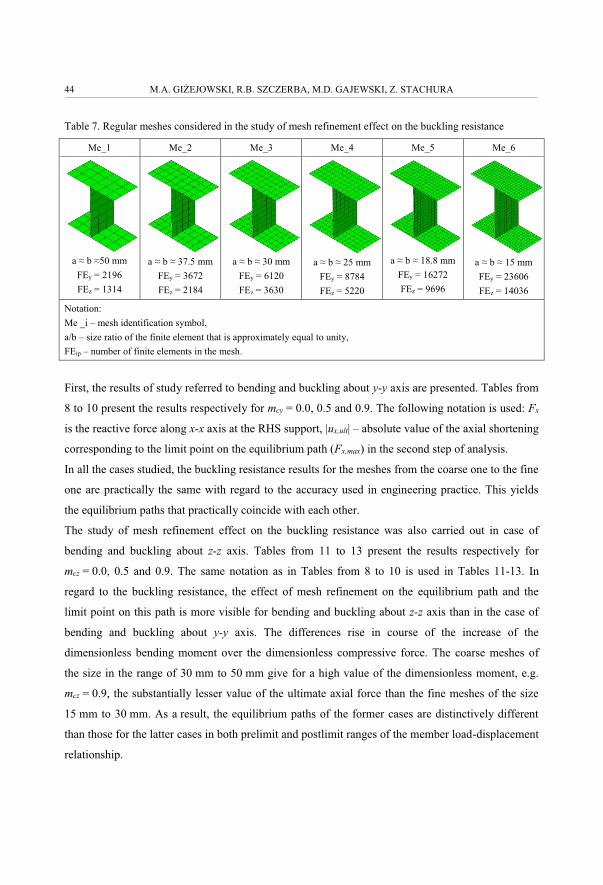
Table 7. Regular meshes considered in the study of mesh refinement effect on the buckling resistance
Me_1 Me_2 Me_3 Me_4 Me_5 Me_6
a ≈ b ≈50 mmFEy = 2196FEz = 1314
a ≈ b ≈ 37.5 mmFEy = 3672FEz = 2184
a ≈ b ≈ 30 mmFEy = 6120FEz = 3630
a ≈ b ≈ 25 mmFEy = 8784FEz = 5220
a ≈ b ≈ 18.8 mmFEy = 16272FEz = 9696
a ≈ b ≈ 15 mmFEy = 23606FEz = 14036
Notation:Me _i – mesh identification symbol, a/b – size ratio of the finite element that is approximately equal to unity,FEip – number of finite elements in the mesh.
First, the results of study referred to bending and buckling about y-y axis are presented. Tables from
8 to 10 present the results respectively for mcy = 0.0, 0.5 and 0.9. The following notation is used: Fx
is the reactive force along x-x axis at the RHS support, |ux,ult| ‒ absolute value of the axial shortening
corresponding to the limit point on the equilibrium path (Fx,max) in the second step of analysis.
In all the cases studied, the buckling resistance results for the meshes from the coarse one to the fine
one are practically the same with regard to the accuracy used in engineering practice. This yields
the equilibrium paths that practically coincide with each other.
The study of mesh refinement effect on the buckling resistance was also carried out in case of
bending and buckling about z-z axis. Tables from 11 to 13 present the results respectively for
mcz = 0.0, 0.5 and 0.9. The same notation as in Tables from 8 to 10 is used in Tables 11-13. In
regard to the buckling resistance, the effect of mesh refinement on the equilibrium path and the
limit point on this path is more visible for bending and buckling about z-z axis than in the case of
bending and buckling about y-y axis. The differences rise in course of the increase of the
dimensionless bending moment over the dimensionless compressive force. The coarse meshes of
the size in the range of 30 mm to 50 mm give for a high value of the dimensionless moment, e.g.
mcz = 0.9, the substantially lesser value of the ultimate axial force than the fine meshes of the size
15 mm to 30 mm. As a result, the equilibrium paths of the former cases are distinctively different
than those for the latter cases in both prelimit and postlimit ranges of the member load-displacement
relationship.
44 M.A. GI�EJOWSKI, R.B. SZCZERBA, M.D. GAJEWSKI, Z. STACHURA
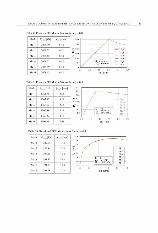
Table 8. Results of FEM simulations for mcy = 0.0
Mesh Fx,max [kN] |ux,ult| [mm]
Me_1 3009.39 6.12
Me_2 3009.32 6.12
Me_3 3009.55 6.12
Me_4 3009.52 6.12
Me_5 3009.49 6.12
Me_6 3009.42 6.12
Table 9. Results of FEM simulations for mcy = 0.5
Mesh Fx,max [kN] |ux,ult| [mm]
Me_1 1364.76 4.08
Me_2 1365.85 4.08
Me_3 1366.59 4.08
Me_4 1366.98 4.08
Me_5 1366.99 4.08
Me_6 1366.89 4.18
Table 10. Results of FEM simulations for mcy = 0.9
Mesh Fx,max [kN] |ux,ult| [mm]
Me_1 387.69 7.18
Me_2 389.84 7.28
Me_3 390.80 7.38
Me_4 391.32 7.48
Me_5 391.73 7.28
Me_6 391.78 7.28
BEAM-COLUMN IN-PLANE RESISTANCE BASED ON THE CONCEPT OF EQUIVALENT... 45

Table 11. Results of FEM simulations for mcz = 0.0
Mesh Fx,max [kN] |ux,ult| [mm]
Me_1 3030.38 3.88
Me_2 3037.59 3.98
Me_3 3040.84 3.98
Me_4 3041.87 3.98
Me_5 3042.84 3.98
Me_6 3043.57 3.98
Table 12. Results of FEM simulations for mcz = 0.5
Mesh Fx,max [kN] |ux,ult| [mm]
Me_1 1743.63 3.78
Me_2 1749.11 3.98
Me_3 1761.49 4.08
Me_4 1764.60 3.98
Me_5 1765.34 4.08
Me_6 1766.91 3.98
Table 13. Results of FEM simulations for mcz = 0.9
Mesh Fx,max [kN] |ux,ult| [mm]
Me_1 262.15 2.88
Me_2 264.05 1.58
Me_3 279.82 1.88
Me_4 279.38 2.28
Me_5 284.72 1.98
Me_6 282.85 2.13
The conducted study gave way to an adoption of meshing that yields more balanced results of FEM
simulations in reference to the calculation time and the accuracy level that is acceptable from an
engineering point of view. In the simulations presented hereafter the dimension of shell finite
elements along the section walls mid-surface contour is taken of a = 30 mm (Me_3) and of
a different value b along the x-x axis, depending upon the member length. This yields the range of
ratio a/b being between 0.91 and 1.00 for bending and buckling about axis y-y and 0.94 and 1.00 for
bending and buckling about axis z-z.
46 M.A. GI�EJOWSKI, R.B. SZCZERBA, M.D. GAJEWSKI, Z. STACHURA

3. RESULTS OF NUMERICAL SIMULATIONS FOR THE IN-PLANE BENDING
AND BUCKLING
3.1. BEAM-COLUMNS SUBJECTED TO AXIAL COMPRESSION
Figs. 3 and 4 present the results for imperfect beam-columns for which the applied moments are
equal to zero. Results correspond to single imperfection profiles, namely, Cases 1, 2a and 2b (see
Tab. 4) and are compared with results obtained with application of Eurocode’s recommendations
[11]. In the figures, the following designations are used: dashed line ‒ results from adopting the
Eurocode’s criteria [11], solid line ‒ Euler's curve, PER ‒ results of elements with perfect geometry
according to [12] (GMNA+ denoted by squares, LBA denoted by diamonds), IMP_1, IMP_2a,
IMP_2b ‒ results of numerical simulations of present study taking into account the appropriate
imperfection profiles (GMNIA denoted by circles and triangles).
a) b)
Fig. 3. Numerical results for pure compression and buckling about y-y axis in case of single imperfection
profile (αy = 0.34); a) IMP_1, b) IMP_2a, IMP_2b
a) b)
Fig. 4. Numerical results for pure compression and buckling about z-z axis in case of single imperfection
profile (αz = 0.49); a) IMP_1, b) IMP_2a, IMP_2b
BEAM-COLUMN IN-PLANE RESISTANCE BASED ON THE CONCEPT OF EQUIVALENT... 47

Comparing the results presented in Figs. 3 and 4 for imperfect and perfect columns, the following
observations can be drawn:
1. Global effect of imperfections modelled by equivalent quantities of the representative
geometrical imperfection profile is important leading to the drastic reduction of the perfect member
buckling resistance.
2. Results of numerical simulations for medium and large values of the slenderness ratio of
imperfect columns with the equivalent imperfection profile according to the lowest LBA mode
(i = 1 in Figs. 3a and 4a) and the amplitude of the Eurocode’s general method are a bit lower than
those based on the analytical buckling curve formulation adopted in [11]. The equivalent
imperfection amplitude is directly proportional to the member section resistance [see Eq. (2.1)]. The
greater difference between the FEM results and those yielding directly from the Eurocode’s
buckling curve formulation is observed for buckling about z-z axis. Such difference results from the
fact that the ratio of the equivalent imperfection amplitude calculated for Mc,ip,Rk = Mpl,ip,Rk and
Mc,ip,Rk = Mel,ip,Rk is for buckling about z-z axis much greater than that referred to buckling about y-y
axis.
3. Results of numerical simulations for low values of the slenderness ratio of imperfect columns
with the equivalent imperfection profile according to the lowest LBA mode (i = 1 in Figs. 3a and
4a) and the amplitude of the Eurocode’s general method are a bit higher than those based on the
analytical buckling curve formulation adopted in EN 1993-1-1 [11]. This results from the fact that
the present study takes the linear strain hardening effect into account in contrast to the Eurocode’s
buckling curve formulation that takes a tri-linear stress-strain model with the yielding plateau and
strain hardening affecting the resistance when the member slenderness ratio is lower than 0.2.
4. Global effect of imperfections represented by equivalent values of the representative geometrical
imperfection profile according to the second lowest LBA mode (i = 2 in Figs. 3b and 4b) is of
a similar tendency as for the imperfection profile according to the lowest LBA mode. It is important
to notice that firstly, the Riks (or Newton-Raphson) incremental-iterative algorithm in the
NLGEOM option used in ABAQUS/Standard cannot detect the effect of bifurcation instability. As
a result, the imperfect column deflects according to the double curvature from the starting point of
Px,d load application up to reaching the limit point on the nonlinear equilibrium path characterizing
the imperfect member response under adopted loading conditions. Secondly, the resistance results
referred to the value of amplitudes based on the slenderness ratio concept are lower than those
based on the energy concept, and closer to the results of Eurocode’s buckling curve formulation
based on the critical force equal to the second lowest bifurcation force.
48 M.A. GI�EJOWSKI, R.B. SZCZERBA, M.D. GAJEWSKI, Z. STACHURA

5. For practical simulations of the buckling resistance of steel members, the imperfection profile
cannot miss the form of initial curvature representing the lowest eigenmode. The imperfection
profile has to be based on the initial curvature representing the lowest eigenmode and successive
modes, if it is necessary.
Figs. 5 and 6 present the results of imperfect columns for which double imperfection profiles are
used, namely Case 1 “+” 2a, and Case 1 “+” 2b (see Table 5) and are compared with outcomes
resulting from the application of Eurocode’s recommendations [11]. In the figures, the following
designations are used: dashed line ‒ results from adopting the Eurocode’s criteria, solid line ‒
Euler's curve, IMP_1,2a, IMP_1,2b ‒ results of numerical simulations of present study taking into
account the appropriate imperfection profiles (GMNIA denoted by circles and triangles).
a) b)
Fig. 5. Numerical results for pure compression and buckling about y-y axis in case of double imperfection
profile (αy = 0.34); a) IMP_1,2a, b) IMP_1,2b
a) b)
Fig. 6. Numerical results for pure compression and buckling about z-z axis in case of double imperfection
profile (αz = 0.49); a) IMP_1,2a, b) IMP_1,2b
BEAM-COLUMN IN-PLANE RESISTANCE BASED ON THE CONCEPT OF EQUIVALENT... 49

Comparing the results presented in Figs. 5 and 6 one can conclude the following:
1. Inclusion of the double imperfection profile and the amplitudes according to the Eurocode’s
general method evaluated on the basis of plastic section resistances results, for slenderness ratios of
around one or less, in a better reproduction of the buckling curves than in case of application of the
single imperfection profile according to the lowest eigenmode.
2. Despite the fact that for the single imperfection profile according to the second lowest mode, the
results obtained for the amplitude based on the slenderness ratio concept are closer to the buckling
curve (the modified Eurocode’s one evaluated analytically for the critical force equal to the second
lowest bifurcation force, i.e. for i = 2), the results of double imperfection profile with the amplitude
based on the energy concept are closer to the original Eurocode’s buckling curve.
3. The general conclusion from the numerical study presented in this section is that the resistance of
real steel structural systems should be based on either:
a) a single imperfection profile according to the lowest eigenmode and its amplitude based on the
elastic section resistance Mc,ip,Rk = Mel,ip,Rk rather than on the section class dependent resistances of
Mc,ip,Rk, for a better accuracy of buckling strength predictions of members with larger values of the
slenderness ratio (over that distinguishing notionally the regions of inelastic and elastic buckling),
or
b) a double imperfection profile according to the combination of the lowest and the second lowest
bifurcation modes, and their amplitudes based on class dependent section resistances Mc,ip,Rk rather
than on the resistance Mc,ip,Rk = Mel,ip,Rk, for a better accuracy of buckling strength predictions of
members with low up to medium values of the slenderness ratio (up to that distinguishing notionally
the regions of inelastic and elastic buckling).
It is important to notice that in the present study of class 1 section members the application of
Mc,ip,Rk = Mpl,ip,Rk is used throughout the FEM simulations.
3.2. BEAM-COLUMNS SUBJECTED TO IN-PLANE BENDING AND BUCKLING
The results of numerical simulations are illustrated graphically by the relationship between the
normalized first-order moment mc,ip = Mip,Ed,max / Mip,pl,Rd and the axial force Nip,max,Ed corresponding
to the limit point on the nonlinear equilibrium path at the ultimate limit state for bending and
buckling about ip axis, normalized with reference to the design plastic resistance of the cross-
section in compression Npl,Rd, i.e. nc,ip = Nip,max,Ed / Npl,Rd. The first order moments
Mip,Ed,max = MIip,Ed,max are used for the graphical illustration of numerical results for both perfect and
imperfect beam-columns. It has to be noted that a comprehensive analysis of the perfect beam-
50 M.A. GI�EJOWSKI, R.B. SZCZERBA, M.D. GAJEWSKI, Z. STACHURA

column resistance with regard to the normalized second-order moment mIIc,ip = MII
ip,Ed,max / Mip,pl,Rd
was presented in [12].
The following figures present the resistance interaction curves. Obtained results are referred to four
different values of the relative flexural slenderness ratio ip� , namely, 0.5 (black); 1.0 (blue); 1.5
(green) and 2.0 (red). Additionally, interaction resistance curve for the relative flexural slenderness
ip� = 0.2 was created (grey), for which the beam-column with perfect geometry was analyzed
(without the effect of imperfections). In the figures, the following designations were adopted:
_1 ‒ geometric imperfection profile corresponding to the lowest bifurcation mode with amplitude
e0,y1 or e0,z1 (solid line with a proper marker), _1,2a and _1,2b ‒ geometric imperfection profile
corresponding to the combination of two lowest eigenmodes with two different values of the second
mode amplitude e0,y2a or e0,z2a (solid line with a proper marker) and e0,y2b or e0,z2b (long-dashed line),
respectively, PER ‒ results of elements with perfect geometry (pale line).
Figs. 7, 8 and 9 correspond to bending and buckling about y-y axis with regard to the single
imperfection profile. Figs. 10, 11 and 12 present the results of similar investigations made available
for bending and buckling about z-z axis. Figs. 7a and 10a, 8a and 11a as well as 9a and 12a show
the results for a single imperfection profile corresponding to the lowest eigenmode (see Table 4,
case 1) evaluated for the amplitude based on Mip,pl,Rd. Figs. from 7b to 12b show the similar results
for a single imperfection profile corresponding to the second lowest eigenmode (see Table 4, cases
2a, 2b). They are compared with the results obtained in [12] for perfect beam-columns (pale line).
a) b)
Fig. 7. Numerical results for bending and buckling about y-y axis in case of UM-Y; a) imperfect elements
with a single imperfection profile IMP_1 (GMNIA), b) imperfect elements with a single imperfection profile
IMP_2a or IMP_2b (GMNIA); PER ‒ perfect elements (GMNA+)
BEAM-COLUMN IN-PLANE RESISTANCE BASED ON THE CONCEPT OF EQUIVALENT... 51

a) b)
Fig. 8. Numerical results for bending and buckling about y-y axis in case of TM-Y;
a) imperfect elements with a single imperfection profile IMP_1 (GMNIA), b) imperfect elements with
a single imperfection profile IMP_2a or IMP_2b (GMNIA); PER ‒ perfect elements (GMNA+)
a) b)
Fig. 9. Numerical results for bending and buckling about y-y axis in case of AM-Y; a) imperfect elements
with a single imperfection profile IMP_1 (GMNIA), b) imperfect elements with a single imperfection profile
IMP_2a or IMP_2b (GMNIA); PER ‒ perfect elements (GMNA+)
a) b)
Fig. 10. Numerical results for bending and buckling about z-z axis in case of UM-Z;
a) imperfect elements with a single imperfection profile IMP_1 (GMNIA), b) imperfect elements with
a single imperfection profile IMP_2a or IMP_2b (GMNIA); PER ‒ perfect elements (GMNA+)
52 M.A. GI�EJOWSKI, R.B. SZCZERBA, M.D. GAJEWSKI, Z. STACHURA

a) b)
Fig. 11. Numerical results for bending and buckling about z-z axis in case of TM-Z; a) imperfect elements
with a single imperfection profile IMP_1 (GMNIA), b) imperfect elements with a single imperfection profile
IMP_2a or IMP_2b (GMNIA); PER ‒ perfect elements (GMNA+)
a) b)
Fig. 12. Numerical results for bending and buckling about z-z axis in case of AM-Z; a) imperfect elements
with a single imperfection profile IMP_1 (GMNIA), b) imperfect elements with a single imperfection profile
IMP_2a or IMP_2b (GMNIA); PER ‒ perfect elements (GMNA+)
Figs. 13, 14 and 15 present the results for double imperfection profiles marked by solid and dashed
lines, respectively for cases e0,ip1“+”e0,ip2a and e0,ip1“+”e0,ip2b (see Table 5) and evaluated for the
amplitudes based also on Mip,pl,Rd. They are compared with numerical results obtained for the
amplitude value e0,ip1 (dotted line) to assess the effect of the higher order eigenmode in combination
with the lowest one on the buckling resistance.
BEAM-COLUMN IN-PLANE RESISTANCE BASED ON THE CONCEPT OF EQUIVALENT... 53

a) b)
Fig. 13. Numerical results for bending and buckling in case of double imperfection profiles IMP_1,2a,
IMP_1,2b (GMNIA) and UM-IP; a) bending and buckling about y-y axis, b) bending and buckling about z-z
axis
a) b)
Fig. 14. Numerical results for bending and buckling in case of double imperfection profiles IMP_1,2a,
IMP_1,2b (GMNIA) and TM-IP; a) bending and buckling about y-y axis, b) bending and buckling about z-z
axis
a) b)
Fig. 15. Numerical results for bending and buckling in case of double imperfection profiles IMP_1,2a,
IMP_1,2b (GMNIA) and AM-IP; a) bending and buckling about y-y axis, b) bending and buckling about z-z
axis
54 M.A. GI�EJOWSKI, R.B. SZCZERBA, M.D. GAJEWSKI, Z. STACHURA

Comparing the results presented in figures shown in this subsection, one can conclude the
following:
1. Global effect of imperfections modelled by equivalent quantities of the representative
geometrical imperfection profile is more important for low vales of bending moments and their
influence on the resistance decreases when the bending stress resultant starts to dominate over the
axial force.
2. The effect of multiple mode imperfection profile on the member resistance is negligible in case
of uniform bending but starts to have a more significant influence on the beam-column behaviour
for nonuniform bending cases that are referred to the higher moment gradient (the lower moment
gradient ratio ψip). For the moment gradient ratio ψip = -1 the difference are the highest and they are
more visible for the medium values of the stress resultants ratio mc,ip / nc (or nc / mc,ip) and contrarily
less visible for dimensionless stress resultants approaching the unit values.
3. The upper bound resistance interaction curve is created by the FEM results of a single
imperfection profile according to the lowest eigenmode while the lower bound of this curve by
numerical results of a double imperfection profile according to the combination of the lowest
eigenmode and the second lowest mode with the amplitude relevant to the buckling length concept.
The results of a double imperfection profile with the amplitude relevant to the energy concept are
placed in between.
4. The results for beam-columns referred to a single imperfection profile corresponding to the
second lowest eigenmode are placed above those for a single imperfection profile corresponding to
the lowest eigenmode.
3.3. COMPARISON OF IMPERFECT BEAM-COLUMN RESISTANCES WITH EUROCODE’S
RECOMMENDATIONS
The results derived from numerical simulations are compared with those of EN 1993-1-1 [11]. In
the figures, the following designations were adopted: _1 ‒ geometric imperfection profile
corresponding to the lowest bifurcation mode with amplitude e0,ip1 (solid line with a proper marker),
_1,2a and _1,2b ‒ geometric imperfection profile corresponding to the combination of two lowest
eigenmodes with two different values of the second mode amplitude e0,ip2, namely e0,ip2a (solid line
with a proper marker) and e0,ip2b (long-dashed line), respectively, EC ‒ results from adopting the
EN 1993-1-1 [11] resistance criteria according to Method 1 or Method 2 (dotted line).
BEAM-COLUMN IN-PLANE RESISTANCE BASED ON THE CONCEPT OF EQUIVALENT... 55

EN 1993-1-1 [11] introduces two methods for the strength verification of beam-columns. The
analytical formulation of interaction resistance according to Eurocode’s Method 1 is regarded a
more accurate approximation of the results of FEM simulations. The comparison of dimensionless
interaction curves given in Figs. 16 to 18 for bending and buckling about y-y axis and in Figs. 19 to
21 for bending and buckling about z-z axis constitutes a verification exercise of the formulation
presented in the current design practice codification [11] since it utilizes EC Method 1 (EC3‒M1).
The accuracy of EC Method 2 may be examined by the comparison of dimensionless interaction
curves given in Figs. 22 to 24 for bending and buckling about y-y axis and in Figs. 25 to 27 for
bending and buckling about z-z axis obtained from FEM simulations and the Eurocode’s analytical
formulation based on the interaction factors corresponding to EC Method 2 (EC3‒M2).
a) b)
Fig. 16. Numerical results for bending and buckling about y-y axis in case of UM-Y (αy = 0.34); a) imperfect
elements with a single imperfection profile IMP_1 (GMNIA), b) imperfect elements with a double
imperfection profile IMP_1,2a or IMP_1,2b (GMNIA); EC ‒ results from adopting the EC3‒M1
a) b)
Fig. 17. Numerical results for bending and buckling about y-y axis in case of TM-Y (αy = 0.34); a) imperfect
elements with a single imperfection profile IMP_1 (GMNIA), b) imperfect elements with a double
imperfection profile IMP_1,2a or IMP_1,2b (GMNIA); EC ‒ results from adopting the EC3‒M1
56 M.A. GI�EJOWSKI, R.B. SZCZERBA, M.D. GAJEWSKI, Z. STACHURA

a) b)
Fig. 18. Numerical results for bending and buckling about y-y axis in case of AM-Y (αy = 0.34);
a) imperfect elements with a single imperfection profile IMP_1 (GMNIA), b) imperfect elements with
a double imperfection profile IMP_1,2a or IMP_1,2b (GMNIA); EC ‒ results from adopting the EC3‒M1
a) b)
Fig. 19. Numerical results for bending and buckling about z-z axis in case of UM-Z (αz = 0.49);
a) imperfect elements with a single imperfection profile IMP_1 (GMNIA), b) imperfect elements with
a double imperfection profile IMP_1,2a or IMP_1,2b (GMNIA); EC ‒ results from adopting the EC3‒M1
a) b)
Fig. 20. Numerical results for bending and buckling about z-z axis in case of TM-Z (αz = 0.49);
a) imperfect elements with a single imperfection profile IMP_1 (GMNIA), b) imperfect elements with
a double imperfection profile IMP_1,2a or IMP_1,2b (GMNIA); EC ‒ results from adopting the EC3‒M1
BEAM-COLUMN IN-PLANE RESISTANCE BASED ON THE CONCEPT OF EQUIVALENT... 57

a) b)
Fig. 21. Numerical results for bending and buckling about z-z axis in case of AM-Z (αz = 0.49);
a) imperfect elements with a single imperfection profile IMP_1 (GMNIA), b) imperfect elements with
a double imperfection profile IMP_1,2a or IMP_1,2b (GMNIA); EC ‒ results from adopting the EC3‒M1
a) b)
Fig. 22. Numerical results for bending and buckling about y-y axis in case of UM-Y (αy = 0.34);
a) imperfect elements with a single imperfection profile IMP_1 (GMNIA), b) imperfect elements with
a double imperfection profile IMP_1,2a or IMP_1,2b (GMNIA); EC ‒ results from adopting the EC3‒M2
a) b)
Fig. 23. Numerical results for bending and buckling about y-y axis in case of TM-Y (αy = 0.34); a) imperfect
elements with a single imperfection profile IMP_1 (GMNIA), b) imperfect elements with a double
imperfection profile IMP_1,2a or IMP_1,2b (GMNIA); EC ‒ results from adopting the EC3‒M2
58 M.A. GI�EJOWSKI, R.B. SZCZERBA, M.D. GAJEWSKI, Z. STACHURA

a) b)
Fig. 24. Numerical results for bending and buckling about y-y axis in case of AM-Y (αy = 0.34);
a) imperfect elements with a single imperfection profile IMP_1 (GMNIA), b) imperfect elements with
a double imperfection profile IMP_1,2a or IMP_1,2b (GMNIA); EC ‒ results from adopting the EC3‒M2
a) b)
Fig. 25. Numerical results for bending and buckling about z-z axis in case of UM-Z (αz = 0.49);
a) imperfect elements with a single imperfection profile IMP_1 (GMNIA), b) imperfect elements with
a double imperfection profile IMP_1,2a or IMP_1,2b (GMNIA); EC ‒ results from adopting the EC3‒M2
a) b)
Fig. 26. Numerical results for bending and buckling about z-z axis in case of TM-Z (αz = 0.49);
a) imperfect elements with a single imperfection profile IMP_1 (GMNIA), b) imperfect elements with
a double imperfection profile IMP_1,2a or IMP_1,2b (GMNIA); EC ‒ results from adopting the EC3‒M2
BEAM-COLUMN IN-PLANE RESISTANCE BASED ON THE CONCEPT OF EQUIVALENT... 59

a) b)
Fig. 27. Numerical results for bending and buckling about z-z axis in case of AM-Z (αz = 0.49);
a) imperfect elements with a single imperfection profile IMP_1 (GMNIA), b) imperfect elements with
a double imperfection profile IMP_1,2a or IMP_1,2b (GMNIA); EC ‒ results from adopting the EC3‒M2
Comparing the results presented in figures presented in this subsection, one can conclude the
following:
1. Generally, resistance interaction curves determined in accordance with EN 1993-1-1 [11] are
situated below those constructed on the basis of FEM simulations, with the exception of the pure
compression (mc,ip = 0) and very small values of mc,ip (see Subsection 3.1 for the extensive
explanation).
2. Resistance interaction curves of EN 1993-1-1 [11] are based on both cross-section resistance
check and stability verification.
3. Very good consistency of results is obtained in case of bending and buckling about y-y axis for
SMY (buckling mode and the beam-column deflected profile under bending moment are alike) and
TMY (buckling mode and the beam-column deflected profile under bending moment are not alike
but of the same sign of displacements). A discrepancy of results may be seen in case of AMY
bending moment diagram, especially for the medium values of the stress resultants ratios mc,ip
(buckling mode and the beam-column deflected profile under bending moment are represented by
two extreme displacement shapes).
4. Taking into account the multiple mode imperfection profile results in a better agreement of EC
and FEM interaction curves.
5. In case of bending and buckling about z-z axis, the differences between EC and FEM interaction
curves are quite visible, especially for the small and medium values of the relative flexural
slenderness .z� In case of the z� = 0.5 resistances based on the application of EN 1993-1-1 [11]
are much smaller than those determined with the use of FEM calculations in the whole range of mcz
60 M.A. GI�EJOWSKI, R.B. SZCZERBA, M.D. GAJEWSKI, Z. STACHURA

and nc. It may result from the fact that in case of bisymmetrical I-shape sections of Class 1 and 2
cross-sections Wz,pl / Wz,el ratio is much greater than that referred to the stronger axis of inertia y-y.
6. Although Method 1 is regarded as the most accurate approximation of the results of FEM
simulations, there are still some visible differences in results obtained with use of EN 1993-1-1 [11]
analytical formulation and numerical FEM based simulations.
7. Taking into account the above mentioned observations it is reasonable to develop an alternative
verification method of the beam-column resistance to that of EN 1993-1-1 [11], especially in case
of elements of Class 1 and 2 cross-sections, that would reduce the discrepancies existing mainly for
members with moment diagrams between those of the standard TM and AM cases.
8. The verification carried out according to Method 2, relevant for members adequately torsionally
and laterally restrained, leads to the results being more conservative than those obtained with use of
interaction factors of Method 1 evaluated for members not susceptible to torsional deformations.
4. CONCLUDING REMARKS
In this paper, the comprehensive study of the geometrical imperfection shape and amplitude on the
resistance of simply supported columns and beam-columns of H-sections is presented for a wide
range of the slenderness ratio. The analysis was done for hot-rolled wide flange HEB 300 section
subjected to both compression and bending about the major and minor principal axes and with
different bending moment distributions (cases denoted by UM, TM, AM) along the member
longitudinal x-x axis. The global resistance curves in all cases were determined on a basis of FEM
simulations using the shell modelling technique and elasto-plasticity constitutive model. Thanks to
that there is no need for division onto the cases in which material behaves elastically (elastic
buckling), material behaves elasto-plastically or plastically. Depending on the slenderness ratio,
cross-section type, boundary conditions, imperfection type, imperfection amplitude value or
material description, the global response of imperfect beam-columns is to be determined accurately.
Various imperfection profiles were applied for the beam-column resistance evaluation and obtained
FEM simulation results in the form of global response were compared with results based on the
Eurocode’s analytical formulations according to Method 1 and Method 2. Results obtained from
GMNIA are based on a imperfection profile for the first buckling mode and the amplitude
determined on the basis of Eq. (2.1) or on a double imperfection profile in which the second lowest
buckling mode is taken with the amplitude according to two alternative concepts, namely based on
the buckling length equivalence and the strain energy equivalence. For a better readability of the
BEAM-COLUMN IN-PLANE RESISTANCE BASED ON THE CONCEPT OF EQUIVALENT... 61

paper, the detailed conclusions are numbered and placed in the text just underneath the figures
corresponding to the verification exercise carried out. Nonetheless, some general conclusion are
recalled hereafter in order to underline the main findings.
In case of pure compression of beam-column members with imperfection profiles being a sum of
the first and second lowest buckling mode gives the results of the buckling resistance comparable to
those obtained in case of a single first buckling mode imperfection profile (both in a good
agreement with predictions according to Eurocode’s buckling curves). On the other hand, in case of
beam-columns subjected to in-plane buckling and bending, the application of double imperfection
profiles leads to the results being quite close to Eurocede predictions for the bending moment
distributions denoted as UM (uniform) and TM (triangular). For the antisymmetrical moment
distribution (AM) there are bigger discrepancies. Thus the conclusion may be formulated that
proper choice of the imperfection profile is strongly related to the member loading pattern.
The results of FEM simulations prove that the imperfection profile should always consist of the
component being alike the lowest buckling mode and if necessary in combination with other
components being represented by higher order buckling modes. It is important to underline that
because of this fact the standard design methods based on the lowest eigenmode imperfection
profile are sufficient for the buckling resistance evaluation in all the cases of members subjected to
a single curvature of second order bending.
From the calculations presented in this study one may conclude that the amplitude of the equivalent
imperfection profile evaluated from Eq. (2.1) should be based rather on the elastic section
properties, regardless the class of the section, than on the class dependent properties. This allows for
general method based predictions of the buckling strength of slender members closer to the
predictions based on the Eurocode’s buckling curve formulation. For inelastic buckling range, the
results presented in this study are higher than the predictions based on the Eurocode’s buckling
curve formulation since the steel constitutive model adopted accounts for the strain hardening
effect. Utilization of the elastic-perfect-plastic constitutive model would lead to a similar accuracy
of predictions, regardless the member slenderness ratio.
62 M.A. GI�EJOWSKI, R.B. SZCZERBA, M.D. GAJEWSKI, Z. STACHURA

REFERENCES
1. ABAQUS Theory manual, Version 6.1, Hibbitt, Karlsson & Sorensen, Inc., Pawtucket, 2000. 2. ABAQUS/Standard User’s manual, Version 6.1, Hibbitt, Karlsson & Sorensen, Inc., Pawtucket, 2000.3. A. Aguero, L. Pallares, F.J. Pallares, “Equivalent geometric imperfection definition in steel structures sensitive
to lateral torsional buckling due to bending moment”, Engineering Structures, 96, pp 41-55, 2015. 4. A. Aguero, L. Pallares, F.J. Pallares, “Equivalent geometric imperfection definition in steel structures sensitive
to flexural and/or torsional buckling due to compression”, Engineering Structures, 96, pp 160-77, 2015. 5. W.E. Ayrton, J. Perry, “On struts”, The Engineer, 62, pp 464-465, 1886. 6. F. Bijlaard, M. Feldmann, J. Naumes, G. Sedlacek, “The “general method” for assessing the out-of-plane
stability of structural members and frames and the comparison with alternative rules in EN 1993 – Eurocode 3 – Part 1-1”, Steel Construction, 3 (1), pp 19-33, 2010.
7. A. Boissonnade, J.-P. Jaspart, J.-P. Muzeau, M. Villette, “New interaction formulae for beam-columns in Eurocode 3: The French–Belgian approach”, Journal of Constructional Steel Research, 60, pp 421-431, 2004.
8. E. Chladny, M. Stujberova, “Frames with unique global and local imperfection in the shape of the elastic buckling mode”, Stahlbau, Part 1 – 82 (8), pp 609-617, 2013; Part 2 – 82 (9), pp 684-695, 2013.
9. W.F. Chen, T. Atsuta, “Theory of Beam-Columns, Vol. 1, In-plane Behavior and Design”, McGraw-Hill, New York, 1976.
10. C. Dou, Y. Pi, “Effects of Geometric Imperfections on Flexural Buckling Resistance of Laterally Braced Columns”, Journal of Structural Engineering, 142 (9), 2016.
11. EN 1993-1-1, Eurocode 3: Design of Steel Structures, Part 1-1: General rules and rules for buildings. Brussels, European Committee for Standardization, 2005.
12. M. Giżejowski, R. Szczerba, M. Gajewski, Z. Stachura, “Buckling resistance assessment of steel I-section beam-columns not susceptible to LT-buckling”, Archives of Civil and Mechanical Engineering, 17 (2), pp 205-221, 2017 (in press).
13. M. Giżejowski, Z. Stachura, “Buckling strength of a steel multi-storey framework according to Eurocode’s general method”, Proceedings of the XIII-th International Conference on Metal Structures, Zielona Gora, Poland, pp 154-155 (e-book on CD: pp 381-391), 2016.
14. M. Giżejowski, Z. Stachura, M. Gajewski, R. Szczerba, “A new method of buckling resistance evaluation of laterally restrained beam-columns”, Proceedings of the XIII-th International Conference on Metal Structures, Zielona Gora, Poland, pp 102-103 (e-book on CD: pp 197-205), 2016.
15. R. Gonçalves, D. Camotim, “On the incorporation of equivalent member imperfections in the in-plane design of steel frames”, Journal of Constructional Steel Research, 61 (9), pp 1226-1240, 2005.
16. R. Greiner, J. Lindner, “Interaction formulae for members subjected to bending and axial compression in Eurocode 3–the Method 2 approach”, Journal of Constructional Steel Research, 62, 757-770, 2006.
17. S. Jemioło, M. Gajewski, “Hyperelasto-plasticity”, Warsaw University of Technology Publishing House, Warsaw, 2014 [in Polish].
18. A.S. Khan, S. Huang, “Continuum Theory of Plasticity”, John Wiley & Sons, Inc., New York, 1995. 19. A. Kozłowski, R. Szczerba, “Design resistance of beam-column according to general method”, Proceedings of
the 7th European Conference on Steel and Composite Structures EUROSTEEL, Naples, Italy, pp 155-156 (full paper – pen-drive 6p.), 2014.
20. A. Lechner, “Flexural buckling of frames according to the new EC3 rules – a comparative, parametric study”, Proceedings of the International colloquium on stability and ductility of steel structures, Lisbon, Portugal, 2006.
21. J. Lubliner, “Plasticity Theory”, Macmillan Publishing Company, New York, 1990. 22. Sz. Pałkowski, “Basis of stability of steel rod structures”, Wyd. Uczelniane PK, Koszalin, 2016 [in Polish].23. F. Papp, “Buckling assessment of steel members through overall imperfection method”, Engineering
Structures, 106, pp 124-136, 2016. 24. F. Papp, A. Rubert, J. Szalai, “DIN EN 1993-1-1 based integrated stability analysis of 2D/3D steel structures”,
Stahlbau, Part 1 – 83 (1), pp 1-15, 2014; Part 2 – 83 (2), pp 122-141, 2014; Part 3 – 83 (5), 325-342, 2014 [in German]
25. K.J.R. Rasmussen, F. de Sena Cardoso, “On the next generation of design specifications for steel structures. Insights and Innovations in Structural Engineering, Mechanics and Computation”, Proceedings of the 6th International Conference on Structural Engineering, Mechanics and Computation, Cape Town, South Africa, 2016.
26. J. Rondal, R. Maquoi, “Le Flambement des Collonnes en Acier”, Notice 1091, Chambre Syndicale des Fabricants de Tubes d’Acier, Paris, France, 1980 [in French].
27. K. Rykaluk,. “Stability problems of metal structures”, Dolnośląskie Wydawnictwo Edukacyjne, Wrocław, 2012 [in Polish].
BEAM-COLUMN IN-PLANE RESISTANCE BASED ON THE CONCEPT OF EQUIVALENT... 63

28. S. Shayan, K.J.R. Rasmussen, H. Zhang, “On the modelling of initial geometric imperfections of steel frames in advanced analysis”, Journal of Constructional Steel Research, 98, pp 167-177, 2014.
29. L. Simões da Silva, L. Marques, C. Rebelo, “Numerical validation of the general method in EC3-1-1 for prismatic members”, Journal of Constructional Steel Research, 66, pp 575-590, 2010.
30. L. Simoes da Silva, R. Simoes, H. Gervasio, “Design of Steel Structures, Eurocode 3: Design of Steel Structures, Part 1-1: General Rules and Rules for Buildings”, ECCS Eurocode Design Manual, Ernst & Sohn, Berlin, 2010.
31. T. Tankova, L. Simões da Silva, L. Marques, A. Andrade, “Proposal of an Ayrton-Perry design methodology for the verification of flexural and lateral-torsional buckling of prismatic beam-columns”, Proceedings of the 8th International Conference on Advances in Steel Structures, Lisbon, Portugal, 2015.
32. A. Taras, “Derivation of DSM-type resistance functions for in-plane global buckling of steel beam-columns”, Journal of Constructional Steel Research, 125, pp 95-113, 2016.
33. N.S. Trahair, M.A. Bradford, D.A. Nethercot, L. Gardner, “The Behaviour and Design of Steel Structures to EC3”, fourth ed., Taylor & Francis, London and New York, 2008.
34. Z. Waszczyszyn, Cz. Cichoń, M. Radwańska, “Finite element method in stability assessment of structures”,Arkady, Warszawa, 1990 [in Polish]
35. S. Weiss, M.A. Giżejowski, “Stability of metal structures. Rod structures”, Arkady, Warszawa, 1991 [in Polish].
36. M. Życzkowski, “Stability of rods and rod structures”, in “Strength of structural elements” (eds. Z. Brzoska, Z. Kączkowski, J. Lipka, Z. Olesiak, M. Życzkowski), vol. IX, chapter III, PWN, Warsaw, 1988.
Received 08.11.2016
Revised 10.12.2016
LIST OF FIGURES AND TABLES:
Fig. 1. Basis for numerical analysis, a) assumed relationship between stress and strain in uniaxial tension
test, b) FE SM model in bending about stronger axis of inertia y-y
Rys. 1. Założenia do analizy numerycznej, a) przyjęta relacja pomiędzy naprężeniem a odkształceniem w
próbie jednoosiowego rozciągania, b) model FE SM przy zginaniu względem osi większej bezwładności y-y
Fig. 2. Considered load cases of simply supported beam-columns of HEB 300 cross-section (ip = y, z)
together with imperfection profiles. Moment diagrams: a) UM-IP, b) TM-IP, c) AM-IP (IP = Y, Z)
Rys. 2. Rozpatrywane przypadki obciążenia swobodnie podpartych elementów ściskanych i zginanych
o przekroju HEB 300 (ip = y, z) łącznie z kształtem imperfekcji. Wykresy momentów: a) UM-IP, b) TM-IP,
c) AM-IP (IP = Y, Z)
Fig. 3. Numerical results for pure compression and buckling about y-y axis in case of single imperfection
profile (αy = 0.34); a) IMP_1, b) IMP_2a, IMP_2b
Rys. 3. Wyniki numeryczne przy czystym ściskaniu i zginaniu względem osi y-y w przypadku pojedynczej
imperfekcji (αy = 0.34); a) IMP_1, b) IMP_2a, IMP_2b
Fig. 4. Numerical results for pure compression and buckling about z-z axis in case of single imperfection
profile (αz = 0.49); a) IMP_1, b) IMP_2a, IMP_2b
Rys. 4. Wyniki numeryczne przy czystym ściskaniu i zginaniu względem osi z-z w przypadku pojedynczej
imperfekcji (αz = 0.49); a) IMP_1, b) IMP_2a, IMP_2b
64 M.A. GI�EJOWSKI, R.B. SZCZERBA, M.D. GAJEWSKI, Z. STACHURA
Fig. 5. Numerical results for pure compression and buckling about y-y axis in case of double imperfection
profile (αy = 0.34); a) IMP_1,2a, b) IMP_1,2b
Rys. 5. Wyniki numeryczne przy czystym ściskaniu i zginaniu względem osi y-y w przypadku podwójnej
imperfekcji (αy = 0.34); a) IMP_1,2a, b) IMP_1,2b
Fig. 6. Numerical results for pure compression and buckling about z-z axis in case of double imperfection
profile (αz = 0.49); a) IMP_1,2a, b) IMP_1,2b
Rys. 6. Wyniki numeryczne przy czystym ściskaniu i zginaniu względem osi z-z w przypadku podwójnej
imperfekcji (αz = 0.49); a) IMP_1,2a, b) IMP_1,2b
Fig. 7. Numerical results for bending and buckling about y-y axis in case of UM-Y; a) imperfect elements
with a single imperfection profile IMP_1 (GMNIA), b) imperfect elements with a single imperfection profile
IMP_2a or IMP_2b (GMNIA); PER ‒ perfect elements (GMNA+)
Rys. 7. Wyniki numeryczne przy zginaniu i wyboczeniu względem osi y-y w przypadku UM-Y; a) elementy
nieidealne z pojedynczą imperfekcją IMP_1 (GMNIA), b) elementy nieidealne z pojedynczą imperfekcją
IMP_2a lub IMP_2b (GMNIA); PER ‒ elementy idealne (GMNA+)
Fig. 8. Numerical results for bending and buckling about y-y axis in case of TM-Y; a) imperfect elements
with a single imperfection profile IMP_1 (GMNIA), b) imperfect elements with a single imperfection profile
IMP_2a or IMP_2b (GMNIA); PER ‒ perfect elements (GMNA+)
Rys. 8. Wyniki numeryczne przy zginaniu i wyboczeniu względem osi y-y w przypadku TM-Y; a) elementy
nieidealne z pojedynczą imperfekcją IMP_1 (GMNIA), b) elementy nieidealne z pojedynczą imperfekcją
IMP_2a lub IMP_2b (GMNIA); PER ‒ elementy idealne (GMNA+)
Fig. 9. Numerical results for bending and buckling about y-y axis in case of AM-Y; a) imperfect elements
with a single imperfection profile IMP_1 (GMNIA), b) imperfect elements with a single imperfection profile
IMP_2a or IMP_2b (GMNIA); PER ‒ perfect elements (GMNA+)
Rys. 9. Wyniki numeryczne przy zginaniu i wyboczeniu względem osi y-y w przypadku AM-Y; a) elementy
nieidealne z pojedynczą imperfekcją IMP_1 (GMNIA), b) elementy nieidealne z pojedynczą imperfekcją
IMP_2a lub IMP_2b (GMNIA); PER ‒ elementy idealne (GMNA+)
Fig. 10. Numerical results for bending and buckling about z-z axis in case of UM-Z; a) imperfect elements
with a single imperfection profile IMP_1 (GMNIA), b) imperfect elements with a single imperfection profile
IMP_2a or IMP_2b (GMNIA); PER ‒ perfect elements (GMNA+)
Rys. 10. Wyniki numeryczne przy zginaniu i wyboczeniu względem osi z-z w przypadku UM-Z; a) elementy
nieidealne z pojedynczą imperfekcją IMP_1 (GMNIA), b) elementy nieidealne z pojedynczą imperfekcją
IMP_2a lub IMP_2b (GMNIA); PER ‒ elementy idealne (GMNA+)
BEAM-COLUMN IN-PLANE RESISTANCE BASED ON THE CONCEPT OF EQUIVALENT... 65
Fig. 11. Numerical results for bending and buckling about z-z axis in case of TM-Z; a) imperfect elements
with a single imperfection profile IMP_1 (GMNIA), b) imperfect elements with a single imperfection profile
IMP_2a or IMP_2b (GMNIA); PER ‒ perfect elements (GMNA+)
Rys. 11. Wyniki numeryczne przy zginaniu i wyboczeniu względem osi z-z w przypadku TM-Z; a) elementy
nieidealne z pojedynczą imperfekcją IMP_1 (GMNIA), b) elementy nieidealne z pojedynczą imperfekcją
IMP_2a lub IMP_2b (GMNIA); PER ‒ elementy idealne (GMNA+)
Fig. 12. Numerical results for bending and buckling about z-z axis in case of AM-Z; a) imperfect elements
with a single imperfection profile IMP_1 (GMNIA), b) imperfect elements with a single imperfection profile
IMP_2a or IMP_2b (GMNIA); PER ‒ perfect elements (GMNA+)
Rys. 12. Wyniki numeryczne przy zginaniu i wyboczeniu względem osi z-z w przypadku AM-Z; a) elementy
nieidealne z pojedynczą imperfekcją IMP_1 (GMNIA), b) elementy nieidealne z pojedynczą imperfekcją
IMP_2a lub IMP_2b (GMNIA); PER ‒ elementy idealne (GMNA+)
Fig. 13. Numerical results for bending and buckling in case of double imperfection profiles IMP_1,2a,
IMP_1,2b (GMNIA) and UM-IP; a) bending and buckling about y-y axis, b) bending and buckling about z-z
axis
Rys. 13. Wyniki numeryczne przy zginaniu i wyboczeniu w przypadku podwójnej imperfekcji IMP_1,2a,
IMP_1,2b (GMNIA) oraz UM-IP; a) zginanie i wyboczenie względem osi y-y, b) zginanie i wyboczenie
względem osi z-z
Fig. 14. Numerical results for bending and buckling in case of double imperfection profiles IMP_1,2a,
IMP_1,2b (GMNIA) and TM-IP; a) bending and buckling about y-y axis, b) bending and buckling about z-z
axis
Rys. 14. Wyniki numeryczne przy zginaniu i wyboczeniu w przypadku podwójnej imperfekcji IMP_1,2a,
IMP_1,2b (GMNIA) oraz TM-IP; a) zginanie i wyboczenie względem osi y-y, b) zginanie i wyboczenie
względem osi z-z
Fig. 15. Numerical results for bending and buckling in case of double imperfection profiles IMP_1,2a,
IMP_1,2b (GMNIA) and AM-IP; a) bending and buckling about y-y axis, b) bending and buckling about z-z
axis
Rys. 15. Wyniki numeryczne przy zginaniu i wyboczeniu w przypadku podwójnej imperfekcji IMP_1,2a,
IMP_1,2b (GMNIA) oraz AM-IP; a) zginanie i wyboczenie względem osi y-y, b) zginanie i wyboczenie
względem osi z-z
Fig. 16. Numerical results for bending and buckling about y-y axis in case of UM-Y (αy = 0.34); a) imperfect
elements with a single imperfection profile IMP_1 (GMNIA), b) imperfect elements with a double
imperfection profile IMP_1,2a or IMP_1,2b (GMNIA); EC ‒ results from adopting the EC3‒M1
Rys. 16. Wyniki numeryczne przy zginaniu i wyboczeniu względem osi y-y w przypadku UM-Y (αy = 0.34);
a) elementy nieidealne z pojedynczą imperfekcją IMP_1 (GMNIA), b) elementy nieidealne z podwójną
imperfekcją IMP_1,2a lub IMP_1,2b (GMNIA); EC ‒ wyniki po przyjęciu EC3‒M1
66 M.A. GI�EJOWSKI, R.B. SZCZERBA, M.D. GAJEWSKI, Z. STACHURA

Fig. 17. Numerical results for bending and buckling about y-y axis in case of TM-Y (αy = 0.34); a) imperfect
elements with a single imperfection profile IMP_1 (GMNIA), b) imperfect elements with a double
imperfection profile IMP_1,2a or IMP_1,2b (GMNIA); EC ‒ results from adopting the EC3‒M1
Rys. 17. Wyniki numeryczne przy zginaniu i wyboczeniu względem osi y-y w przypadku TM-Y (αy = 0.34);
a) elementy nieidealne z pojedynczą imperfekcją IMP_1 (GMNIA), b) elementy nieidealne z podwójną
imperfekcją IMP_1,2a lub IMP_1,2b (GMNIA); EC ‒ wyniki po przyjęciu EC3‒M1
Fig. 18. Numerical results for bending and buckling about y-y axis in case of AM-Y (αy = 0.34); a) imperfect
elements with a single imperfection profile IMP_1 (GMNIA), b) imperfect elements with a double
imperfection profile IMP_1,2a or IMP_1,2b (GMNIA); EC ‒ results from adopting the EC3‒M1
Rys. 18. Wyniki numeryczne przy zginaniu i wyboczeniu względem osi y-y w przypadku AM-Y (αy = 0.34);
a) elementy nieidealne z pojedynczą imperfekcją IMP_1 (GMNIA), b) elementy nieidealne z podwójną
imperfekcją IMP_1,2a lub IMP_1,2b (GMNIA); EC ‒ wyniki po przyjęciu EC3‒M1
Fig. 19. Numerical results for bending and buckling about z-z axis in case of UM-Z (αz = 0.49); a) imperfect
elements with a single imperfection profile IMP_1 (GMNIA), b) imperfect elements with a double
imperfection profile IMP_1,2a or IMP_1,2b (GMNIA); EC ‒ results from adopting the EC3‒M1
Rys. 19. Wyniki numeryczne przy zginaniu i wyboczeniu względem osi z-z w przypadku UM-Z (αz = 0.49);
a) elementy nieidealne z pojedynczą imperfekcją IMP_1 (GMNIA), b) elementy nieidealne z podwójną
imperfekcją IMP_1,2a lub IMP_1,2b (GMNIA); EC ‒ wyniki po przyjęciu EC3‒M1
Fig. 20. Numerical results for bending and buckling about z-z axis in case of TM-Z (αz = 0.49); a) imperfect
elements with a single imperfection profile IMP_1 (GMNIA), b) imperfect elements with a double
imperfection profile IMP_1,2a or IMP_1,2b (GMNIA); EC ‒ results from adopting the EC3‒M1
Rys. 20. Wyniki numeryczne przy zginaniu i wyboczeniu względem osi z-z w przypadku TM-Z (αz = 0.49);
a) elementy nieidealne z pojedynczą imperfekcją IMP_1 (GMNIA), b) elementy nieidealne z podwójną
imperfekcją IMP_1,2a lub IMP_1,2b (GMNIA); EC ‒ wyniki po przyjęciu EC3‒M1
Fig. 21. Numerical results for bending and buckling about z-z axis in case of AM-Z (αz = 0.49); a) imperfect
elements with a single imperfection profile IMP_1 (GMNIA), b) imperfect elements with a double
imperfection profile IMP_1,2a or IMP_1,2b (GMNIA); EC ‒ results from adopting the EC3‒M1
Rys. 21. Wyniki numeryczne przy zginaniu i wyboczeniu względem osi z-z w przypadku AM-Z (αz = 0.49);
a) elementy nieidealne z pojedynczą imperfekcją IMP_1 (GMNIA), b) elementy nieidealne z podwójną
imperfekcją IMP_1,2a lub IMP_1,2b (GMNIA); EC ‒ wyniki po przyjęciu EC3‒M1
Fig. 22. Numerical results for bending and buckling about y-y axis in case of UM-Y (αy = 0.34); a) imperfect
elements with a single imperfection profile IMP_1 (GMNIA), b) imperfect elements with a double
imperfection profile IMP_1,2a or IMP_1,2b (GMNIA); EC ‒ results from adopting the EC3‒M2
Rys. 22. Wyniki numeryczne przy zginaniu i wyboczeniu względem osi y-y w przypadku UM-Y (αy = 0.34);
a) elementy nieidealne z pojedynczą imperfekcją IMP_1 (GMNIA), b) elementy nieidealne z podwójną
imperfekcją IMP_1,2a lub IMP_1,2b (GMNIA); EC ‒ wyniki po przyjęciu EC3‒M2
BEAM-COLUMN IN-PLANE RESISTANCE BASED ON THE CONCEPT OF EQUIVALENT... 67
Fig. 23. Numerical results for bending and buckling about y-y axis in case of TM-Y (αy = 0.34); a) imperfect
elements with a single imperfection profile IMP_1 (GMNIA), b) imperfect elements with a double
imperfection profile IMP_1,2a or IMP_1,2b (GMNIA); EC ‒ results from adopting the EC3‒M2
Rys. 23. Wyniki numeryczne przy zginaniu i wyboczeniu względem osi y-y w przypadku TM-Y (αy = 0.34);
a) elementy nieidealne z pojedynczą imperfekcją IMP_1 (GMNIA), b) elementy nieidealne z podwójną
imperfekcją IMP_1,2a lub IMP_1,2b (GMNIA); EC ‒ wyniki po przyjęciu EC3‒M2
Fig. 24. Numerical results for bending and buckling about y-y axis in case of AM-Y (αy = 0.34); a) imperfect
elements with a single imperfection profile IMP_1 (GMNIA), b) imperfect elements with a double
imperfection profile IMP_1,2a or IMP_1,2b (GMNIA); EC ‒ results from adopting the EC3‒M2
Rys. 24. Wyniki numeryczne przy zginaniu i wyboczeniu względem osi y-y w przypadku AM-Y (αy = 0.34);
a) elementy nieidealne z pojedynczą imperfekcją IMP_1 (GMNIA), b) elementy nieidealne z podwójną
imperfekcją IMP_1,2a lub IMP_1,2b (GMNIA); EC ‒ wyniki po przyjęciu EC3‒M2
Fig. 25. Numerical results for bending and buckling about z-z axis in case of UM-Z (αz = 0.49); a) imperfect
elements with a single imperfection profile IMP_1 (GMNIA), b) imperfect elements with a double
imperfection profile IMP_1,2a or IMP_1,2b (GMNIA); EC ‒ results from adopting the EC3‒M2
Rys. 25. Wyniki numeryczne przy zginaniu i wyboczeniu względem osi z-z w przypadku UM-Z (αz = 0.49);
a) elementy nieidealne z pojedynczą imperfekcją IMP_1 (GMNIA), b) elementy nieidealne z podwójną
imperfekcją IMP_1,2a lub IMP_1,2b (GMNIA); EC ‒ wyniki po przyjęciu EC3‒M2
Fig. 26. Numerical results for bending and buckling about z-z axis in case of TM-Z (αz = 0.49); a) imperfect
elements with a single imperfection profile IMP_1 (GMNIA), b) imperfect elements with a double
imperfection profile IMP_1,2a or IMP_1,2b (GMNIA); EC ‒ results from adopting the EC3‒M2
Rys. 26. Wyniki numeryczne przy zginaniu i wyboczeniu względem osi z-z w przypadku TM-Z (αz = 0.49);
a) elementy nieidealne z pojedynczą imperfekcją IMP_1 (GMNIA), b) elementy nieidealne z podwójną
imperfekcją IMP_1,2a lub IMP_1,2b (GMNIA); EC ‒ wyniki po przyjęciu EC3‒M2
Fig. 27. Numerical results for bending and buckling about z-z axis in case of AM-Z (αz = 0.49); a) imperfect
elements with a single imperfection profile IMP_1 (GMNIA), b) imperfect elements with a double
imperfection profile IMP_1,2a or IMP_1,2b (GMNIA); EC ‒ results from adopting the EC3‒M2
Rys. 27. Wyniki numeryczne przy zginaniu i wyboczeniu względem osi z-z w przypadku AM-Z (αz = 0.49);
a) elementy nieidealne z pojedynczą imperfekcją IMP_1 (GMNIA), b) elementy nieidealne z podwójną
imperfekcją IMP_1,2a lub IMP_1,2b (GMNIA); EC ‒ wyniki po przyjęciu EC3‒M2
Tab. 1. List of member lengths with corresponding slenderness ratios considered in numerical simulations
Tab. 1. Wykaz długości prętów odpowiadających smukłościom rozważanym w symulacjach numerycznych
Tab. 2. Load cases considered
Tab. 2. Rozważane przypadki obciążeń
68 M.A. GI�EJOWSKI, R.B. SZCZERBA, M.D. GAJEWSKI, Z. STACHURA

Tab. 3. Amplitudes of first mode imperfection profile (αy = 0.34, αz = 0.49)
Tab. 3. Amplitudy pierwszej postaci imperfekcji (αy = 0.34, αz = 0.49)
Tab. 4. Imperfection profiles for the single imperfection profile
Tab. 4. Kształty imperfekcji pojedynczej imperfekcji
Tab. 5. Imperfection profile combinations for the double imperfection profile
Tab. 5. Kombinacje kształtów imperfekcji dla podwójnej imperfekcji
Tab. 6. Parameters of beam-columns considered in the study of mesh refinement effect on the buckling
resistance
Tab. 6. Parametry elementów ściskanych i zginanych przyjętych do badania wpływu gęstości siatki na
nośność wyboczeniową
Tab. 7. Regular meshes considered in the study of mesh refinement effect on the buckling resistance
Tab. 7. Siatki o układzie regularnym rozważane przy badaniu wpływu gęstości siatki na nośność
wyboczeniową
Tab. 8. Results of FEM simulations for mcy = 0.0
Tab. 8. Wyniki symulacji FEM przy mcy = 0.0
Tab. 9. Results of FEM simulations for mcy = 0.5
Tab. 9. Wyniki symulacji FEM przy mcy = 0.5
Tab. 10. Results of FEM simulations for mcy = 0.9
Tab. 10. Wyniki symulacji FEM przy mcy = 0.9
Tab. 11. Results of FEM simulations for mcz = 0.0
Tab. 11. Wyniki symulacji FEM przy mcz = 0.0
Tab. 12. Results of FEM simulations for mcz = 0.5
Tab. 12. Wyniki symulacji FEM przy mcz = 0.5
Tab. 13. Results of FEM simulations for mcz = 0.9
Tab. 13. Wyniki symulacji FEM przy mcz = 0.9
BEAM-COLUMN IN-PLANE RESISTANCE BASED ON THE CONCEPT OF EQUIVALENT... 69

NOŚNOŚĆ ELEMENTÓW STALOWYCH ŚCISKANYCH I ZGINANYCH BEZ ZWICHRZENIA NA PODSTAWIE
KONCEPCJI RÓWNOWAŻNYCH IMPERFEKCJI GEOMETRYCZNYCH
Słowa kluczowe: dwuteownik stalowy, zginanie i ściskanie, nośność na wyboczenie giętne, równoważne imperfekcje geometryczne, modelowanie FEM
STRESZCZENIE:
W artykule przedstawiono obszerne studium numeryczne dotyczące wpływu kształtu i amplitudy imperfekcji
o charakterze geometrycznym na nośność swobodnie podpartych elementów ściskanych i zginanych bez zwichrzenia
o przekrojach dwuteowych bisymetrycznych walcowanych typu HEB. Imperfekcje przyjęto zgodnie z koncepcją
równoważnych imperfekcji geometrycznych (która ujmuje zbiorczo zarówno wpływ losowych imperfekcji
geometrycznych jak również materiałowych różnych typów) w odniesieniu do tak zwanej eurokodowej metody ogólnej
[11].
Zgodnie z koncepcją metody ogólnej linia wstępnego wygięcia odpowiada skalowanej formie sprężystego wyboczenia,
stowarzyszonego z wektorem własnym ze sprężystej analizy wyboczeniowej (LBA). Należy jednak zwrócić uwagę, że
rozważenie tylko pojedynczej imperfekcji odpowiadającej pierwszej postaci wyboczenia może w niektórych układach
konstrukcyjnych prowadzić do błędów w oszacowaniu ich nośności. W analizie powinno się uwzględnić kombinację
imperfekcji geometrycznych odpowiadających pierwszej podstawowej i wyższym postaciom wyboczenia [28].
W artykule rozważono wpływ imperfekcji odpowiadających dwóm najniższym postaciom wyboczenia, rozważanych
oddzielnie jak również w ich kombinacji liniowej. Amplitudę równoważnej imperfekcji geometrycznej odpowiadającej
pierwszemu wektorowi własnemu z analizy LBA wyznaczono zgodnie z zaleceniami metody ogólnej zgodnie ze
wzorem (2.1), natomiast amplitudę odpowiadającej drugiej postaci wyboczenia wyznaczono wykorzystując dwa
podejścia [14], z których pierwsze związane jest z długością wyboczeniowej pręta, zaś drugie bazuje na koncepcji
równoważności energetycznej.
Analizy przeprowadzono na prętach stężonych bocznie i przeciwskrętnie poddanych równoczesnemu ściskaniu
i jednokierunkowemu zginaniu względem obu głównych osi bezwładności. Rozważono trzy różne rozkłady wzdłuż osi
x-x wykresu momentu zginającego wywołanego zginaniem momentami skupionymi na końcach pręta: stały
symetryczny (UM), zmienny trójkątny (TM) oraz zmienny antysymetryczny (AM). Modele numeryczne rozważanych
prętów wykonano w programie ABAQUS/Standard z użyciem liniowych, prostokątnych elementów powłokowych typu
S4R (ze zredukowanym całkowaniem) [1, 2]. W ramach pracy, na wybranych przykładach prętów przeprowadzono
badanie wpływu gęstości siatki MES na przebieg ścieżki równowagi i otrzymaną na jej podstawie nośność pręta przy
ściskaniu i zginaniu. Do opisu charakterystyki przyjętej stali konstrukcyjnej S 235 wykorzystano sprężysto-plastyczny
model materiału ze wzmocnieniem izotropowym. Dzięki przyjęciu takiego modelu materiału nie ma potrzeby
rozdzielania zadań na przypadki różnej fazy pracy materiału: sprężystej, sprężysto-plastycznej oraz plastycznej.
Obliczenia numeryczne do wyznaczenia nośności przy ściskaniu oraz ściskaniu i zginaniu elementów imperfekcyjnych
wykonano z wykorzystaniem analizy geometrycznie i materiałowo nieliniowej (GMNIA) z imperfekcją pojedynczą
odpowiadającą pierwszej lub drugiej postaci wyboczenia z analizy LBA lub imperfekcją podwójną odpowiadającą
kombinacji liniowej dwóch pierwszych wektorów własnych. W przypadku prętów o geometrii idealnej wykorzystano
analizę geometrycznie i materiałowo nieliniową z imperfekcją o kształtach i rodzajach analogicznych jak przyjętych
w odniesieniu do elementów nieidealnych, lecz o nieskończenie małej amplitudzie (GMNA+). Przeprowadzone
70 M.A. GI�EJOWSKI, R.B. SZCZERBA, M.D. GAJEWSKI, Z. STACHURA

w programie ABAQUS/Standard analizy GMNA+ i GMNIA zostały wykonane w ramach umiarkowanie dużych
deformacji, tj. przy wykorzystaniu opcji NLGEOM [1, 2].
Globalny efekt wpływu imperfekcji na nośność i zachowanie się słupów i elementów zginanych zilustrowano
porównując nośności elementów nieidealnych z ich odpowiednikami o geometrii idealnej. Wyniki porównań
zaprezentowano na rysunkach w formie wykresów przedstawiających krzywe graniczne nośności prętów ściskanych
i zginanych w bezwymiarowych współrzędnych, z których oś rzędnych opisuje proporcję maksymalnej siły ściskającej
do nośności przekroju na ściskanie, natomiast oś odciętych opisuje proporcję maksymalnego momentu zginającego
(I rzędu) do nośności przekroju na zginanie.
W dalszej części pracy, wyniki otrzymane z analiz numerycznych dotyczących ściskanych i zginanych elementów
imperfekcyjnych porównano z krzywymi granicznymi nośności wyznaczonymi zgodnie z eurokodowymi formułami
interakcyjnymi [11] przyjmując współczynniki interakcyjne dwoma alternatywnymi metodami ‒ Metodą 1 (Rys. 16-21)
oraz Metodą 2 (Rys. 22-27).
W celu lepszej czytelności artykułu, szczegółowe wnioski dotyczące poszczególnych analiz ponumerowano
i umieszczono na końcu tekstu (pod rysunkami) każdego z podpunktów do punktu 3. Mimo to, niektóre ogólne wnioski
przywołano w podsumowaniu artykułu w celu podkreślenia najważniejszych ustaleń wynikających z przeprowadzanych
badań.
W przypadku słupów osiowo ściskanych, otrzymane z analiz numerycznych nośności na wyboczenie po przyjęciu
podwójnej imperfekcji odpowiadającej kombinacji liniowej dwóch pierwszych wektorów własnych otrzymanych
z analizy LBA są porównywalne do nośności słupów z pojedynczą imperfekcją odpowiadającej pierwszej postaci
wyboczenia. Wyniki obliczeń numerycznych z obu modeli imperfekcji są zbliżone do eurokodowych krzywych
wyboczeniowych [11]. Z drugiej strony, w przypadku elementów poddanych jednoczesnemu ściskaniu i zginaniu
w płaszczyźnie wyboczenia giętnego, o ile w odniesieniu do stałego (UM) i trójkątnego (TM) rozkładu wykresu
momentu zginającego przyjęcie podwójnej imperfekcji prowadzi do rezultatów bliskich otrzymanym z normowych
formuł analitycznych [11], o tyle w odniesieniu do antysymetrycznego (AM) rozkładu wykresu momenty zginającego
wyniki obliczeń numerycznych dość istotnie różnią się od otrzymanych zgodnie z eurokodowymi formułami
interakcyjnymi [11]. Oznacza to, że właściwy wybór imperfekcji jest silnie związany ze schematem obciążenia pręta.
Otrzymane wyniki obliczeń numerycznych dowodzą, że kształt imperfekcji powinien zawsze odpowiadać pierwszej
najniższej postaci wyboczenia, a jeżeli jest to konieczne (np. z uwagi na schemat obciążenia) to powinien również
uwzględniać kombinację z innymi wyższymi formami wyboczenia. Należy zwrócić uwagę, że eurokodowe formuły
analityczne do określania nośności elementów [11] bazują tylko i wyłącznie na imperfekcji odpowiadającej pierwszej
najniższej postaci utraty stateczności.
Na podstawie zaprezentowanych w artykule obliczeń i analiz można stwierdzić, że amplituda równoważnych
imperfekcji geometrycznych opisana wzorem (2.1) powinna bazować na sprężystych cechach przekroju zamiast na
cechach przekroju zależnych od jego klasy. Takie założenie pozwoli w obliczeniach numerycznych z wykorzystaniem
analizy GMNIA otrzymać wyniki bliższe do wyznaczonych z eurokodowych formuł interakcyjnych [11], szczególnie
w odniesieniu do prętów smukłych.
BEAM-COLUMN IN-PLANE RESISTANCE BASED ON THE CONCEPT OF EQUIVALENT... 71