Embed Size (px)
Citation preview

Master Thesis
Bearing Behaviour of Shallow
Foundations Under Heavy Train Load
Nelson García Iglesias
Luleå University of Technology
Department of Civil, Environmental and Natural Resources Engineering
2019

Acknowledgements
2

Acknowledgements
3
ACKNOWLEDGEMENTS
The present work is the end of the master studies in Mining engineering which I had the
opportunity to finish in the Luleå University of Technology Soil Mechanics department.
In first place, I would like to thank my supervisor and examiner, Professor Jan Laue who
has guided me with his knowledge and experience during the development of this thesis.
Finally, I would also like to thank Per Gunnvard, PhD student in the Soil Mechanics
department of Luleå University of Technology; who helped me with his expertise in the finite
element program Plaxis.
Luleå, June 2019
Nelson García Iglesias

Abstract
4
ABSTRACT
Foundations related to slopes are commonly found holding railway bridges. Traditionally
this type of foundations is assessed from a foundation’s static point of view and with very
conservative factors of safety. The bearing behaviour of this foundations is not well studied
yet, neither how cyclic loads affect it since these loads are normally neglected. The aim of this
thesis is to get a better understanding of the bearing behaviour of foundations related to
slopes under heavy train loads in static and dynamic conditions with the help of the finite
element program Plaxis.
The models have been built regarding a square foundation of 2,8 m side and 1,14 m of
embedment. This foundation will be placed in top and in the middle of a sand slope. 20º and
30º angle slopes are considered. The same models are made with the foundation’s
embedment doubled. To all the models, bearing capacity calculations are performed from an
analytical and numerical point of view. In addition, the models are cyclically loaded (along 100
cycles) in three ways: first for the foundations with the initial embedment, a load keeping a
ratio of 3,7 between maximum bearing capacity and applied load is used; for the cases with
double embedment a calculated load form a train passing through the bridge is placed; finally,
in the case of double embedment and foundation on top of a 20º slope the horizontal force
and momentum generated by the train braking is also added to the foundation.
From the ultimate bearing capacity calculations, it is seen that a local shear failure is
present in all cases. In situations with bigger slope angles and the foundation situated in the
middle of the slope a combination of local shear failure and slope failure is present. The main
parameter affecting the bearing capacity is the slope angle, bigger slope angles reduce
significantly the bearing capacity. Positions in the middle of the slope and bigger embedment
deals higher bearing capacities.
When taking a look to the cyclic models a punching like failure is developing in all cases,
combined with the start of a slope failure in cases with the foundation in the middle of a 30º
angle slope. In all cases the vertical displacement along the cycles presents an inflexion point
which separates an initial slower settlement speed from the bigger settlement speed after the
inflexion. This interesting point is related with the generation of an active area under the
foundation. The amplitude of the plastic deformation along the cycles follows the same patter
for all cases, it increases until the inflexion point for staying constant after it. The speed of
settlement is affected mainly by the slope angle.

Abstract
5
TABLE OF CONTENTS
Acknowledgements ........................................................................................................................ 3
Abstract ........................................................................................................................................... 4
1 Introduction ............................................................................................................................ 7
2 Background and Motivation ................................................................................................... 8
2.1 Traditional Bearing Capacity Calculations ..................................................................... 8
2.2 Bearing Capacity Problem vs Slope Stability Problem. ................................................ 13
2.3 Strain Accumulation Under Cyclic Loading .................................................................. 13
2.4 Failure Behaviour of Horizontally Loaded Foundations in Slopes ............................... 14
2.5 Small Strain Hardening Soil Model............................................................................... 15
2.6 Phi-C Reduction Calculation ......................................................................................... 16
2.7 Aim and Objectives....................................................................................................... 17
3 Methodology ........................................................................................................................ 18
3.1 Ultimate Bearing Capacity: Analytical Methods .......................................................... 18
3.2 Plaxis Models Build ....................................................................................................... 20
3.3 Ultimate Bearing Capacity Plaxis.................................................................................. 22
3.4 Cyclic Loading Models .................................................................................................. 22
3.4.1 Calculation of Vertical Train Load ........................................................................ 22
3.4.2 Calculation of Horizontal Train Load .................................................................... 24
3.4.3 Constant Force Ratio Loading .............................................................................. 24
3.4.4 Real Force Loading ............................................................................................... 24
3.4.5 Plaxis Modelling for Cyclic Loading ...................................................................... 25
4 Results and Analysis ............................................................................................................. 26
4.1 Ultimate Bearing Capacity ............................................................................................ 26
4.1.1 Input ..................................................................................................................... 26
4.1.2 Calculations .......................................................................................................... 26
4.1.3 Output .................................................................................................................. 27
4.2 Cyclic Loading: Constant Vertical Force Ratio .............................................................. 49
4.2.1 Input ..................................................................................................................... 49
4.2.2 Output .................................................................................................................. 49
4.3 Cyclic Load: Vertical Real Load ..................................................................................... 63
4.3.1 Input ..................................................................................................................... 63
4.3.2 Output .................................................................................................................. 63
4.4 Cyclic Loading: Vertical and Horizontal Real Load ....................................................... 82
4.4.1 Input ..................................................................................................................... 82

Abstract
6
4.4.2 Output .................................................................................................................. 82
4.5 Analysis of the Results .................................................................................................. 90
4.5.1 Cyclic Loading with Vertical Load ......................................................................... 92
4.5.2 Cyclic Loading with Horizontal and Vertical Load ................................................ 95
5 Discussion ............................................................................................................................. 97
5.1 Bearing Capacity ........................................................................................................... 97
5.2 Cyclic Vertical Loading .................................................................................................. 99
5.3 Cyclic Vertical and Horizontal Loading ....................................................................... 101
6 Conclusion and Future Work .............................................................................................. 103
7 References .......................................................................................................................... 104
Appendix I: Soil Model Selection ................................................................................................ 106
Appendix II: Load Control vs Prescribed Displacement ............................................................. 108
Appendix III: Boundary effects ................................................................................................... 113
Appendix IV: Ultimate Bearing Capacity, Shear Surfaces Development ................................... 116

Introduction
7
1 INTRODUCTION
Bridges supported by foundations located close or in slopes is not an uncommon find in
railway lines. This generates a relation between the slope and the foundation in which both
are affected by the others characteristics, changing their isolated ability to support load
without failure.
Traditionally, these problems have been assessed with static calculations that combine
bearing capacity of foundations theories and slope stability. These calculations are also
supported by very conservative factors of safety. Many bridge foundations falling into this
category which have been calculated with these methods are in use today. With time the load
of the trains has been increased leading to a reduction in the safety of these foundations and
making them deal with heavy loads.
It can be said that the failure mechanism of this problem is still not fully studied in order
to understand what kind of failure and how it develops under the heavy load of the foundation
and the slope characteristics.
Other topic traditionally disregarded is the cyclic load that the trains generate when they
travel through the bridge as well as the horizontal forces generated due to braking. With
enough number of cycles and the added effect of the big loads it can change the bearing
behaviour of the foundation in relation to a static situation helping to trigger a failure in the
foundation – slope system.
The present work studies this topic from a theoretical point of view, analysing the static
bearing capacity and developed failures in several foundation – slope cases under heavy loads.
A cyclic analysis of the same cases will be performed as well to see the differences with the
static situation and how the cyclic load affects the bearing capacity and failure mechanisms.
Static and cyclic situations will be studied developing finite element models of the cases in the
program Plaxis.

Background and Motivation
8
2 BACKGROUND AND MOTIVATION
2.1 TRADITIONAL BEARING CAPACITY CALCULATIONS One of the most popular bearing capacity theories is the one developed by Karl Terzaghi.
He considers the soil to be in elastic equilibrium before placing any load. Once the load is
applied and until a certain amount of it, the soil is still in elastic conditions. If the load is
increased more, the soil enters a state of plastic equilibrium (Terzaghi, 1943)
In the case when the soil’s plastic flow during loading is preceded by a very small strain,
general shear failure takes place. In this case the foundation has very few settlements until
failure. If the strain that takes place before the failure is big, local shear failure takes place.
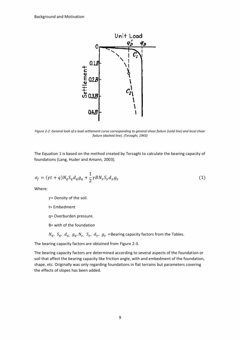
Showing important settlements before failure (Terzaghi, 1943). Figure 2-2 represents the
general look of the load – settlement curve related with both failure cases. General shear
failure surfaces are developed from the edges of the footing all the way until the surface,
ground surface heave is normally present in both sides of the foundation (Figure 2-1, a). In the
case of local shear failure, a state of plastic equilibrium is not fully developed, therefor the
failure surfaces do not reach the surface, heave is slightly present (Figure 2-1, b) (Knappett and
Craig, 2012).
Figure 2-1: General shear failure of a shallow foundation (a) and local shear failure of a shallow foundation (b). (M. Das 2011)
Background and Motivation
9
Figure 2-2: General look of a load settlement curve corresponding to general shear failure (solid line) and local shear failure (dashed line). (Terzaghi, 1943)
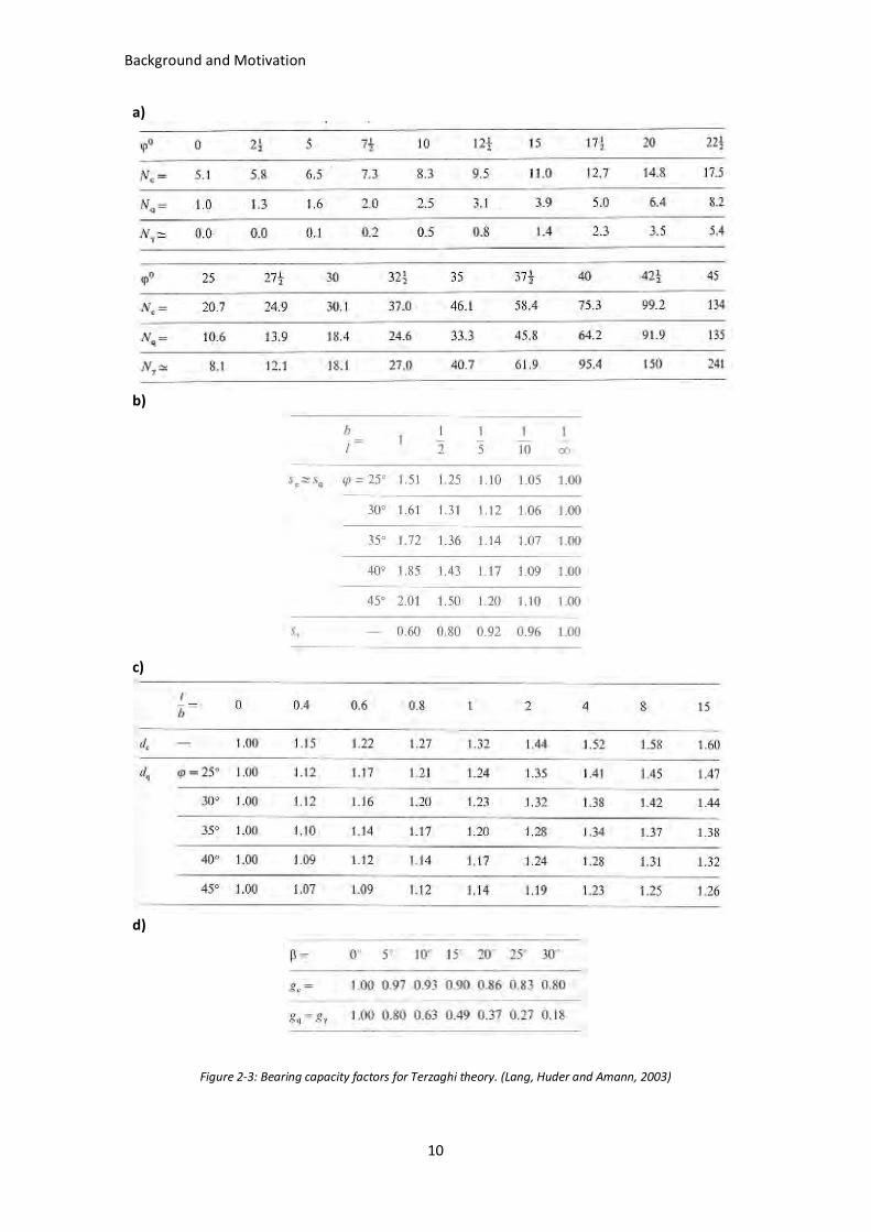
The Equation 1 is based on the method created by Terzaghi to calculate the bearing capacity of
foundations (Lang, Huder and Amann, 2003).
𝜎𝑓 = (𝛾𝑡 + 𝑞)𝑁𝑞𝑆𝑞𝑑𝑞𝑔𝑞 +1
2𝛾𝐵𝑁𝛾𝑆𝛾𝑑𝛾𝑔𝛾 (1)
Where:
𝛾= Density of the soil.
t= Embedment
q= Overburden pressure.
B= with of the foundation
𝑁𝑞 , 𝑆𝑞 , 𝑑𝑞, 𝑔𝑞 , 𝑁𝛾, 𝑆𝛾 , 𝑑𝛾 , 𝑔𝛾 =Bearing capacity factors from the Tables.
The bearing capacity factors are obtained from Figure 2-3.
The bearing capacity factors are determined according to several aspects of the foundation or
soil that affect the bearing capacity like friction angle, with and embedment of the foundation,
shape, etc. Originally was only regarding foundations in flat terrains but parameters covering
the effects of slopes has been added.
Background and Motivation
10
a)
b)
c)
d)
Figure 2-3: Bearing capacity factors for Terzaghi theory. (Lang, Huder and Amann, 2003)
Background and Motivation
11
Meyerhof also developed a bearing capacity theory which he combined with slope
stability (Meyerhof, 1957) for foundations on top and in slopes. He provides methods of
calculating bearing capacities in pure cohesive and pure frictional soils, as well as a combined
way for soils in between of this range.
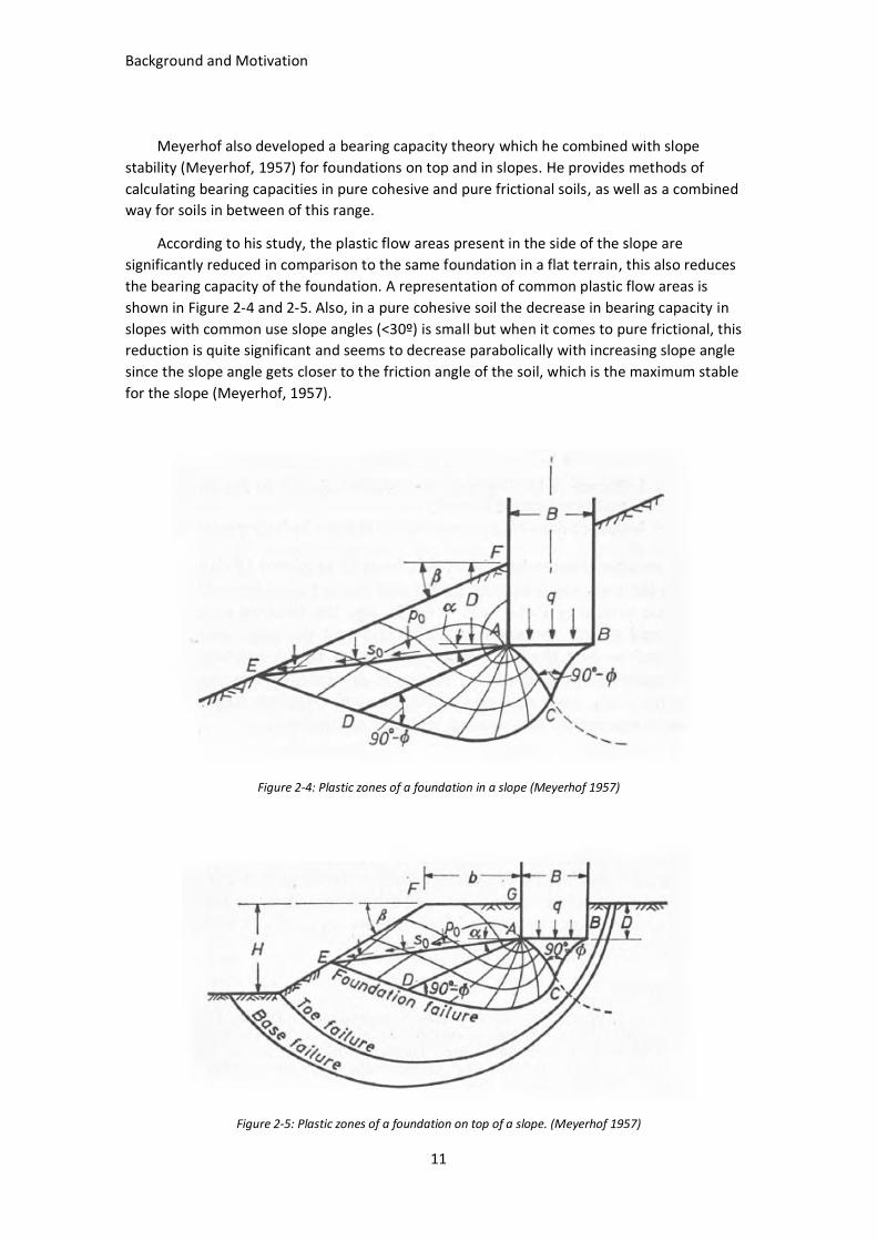
According to his study, the plastic flow areas present in the side of the slope are
significantly reduced in comparison to the same foundation in a flat terrain, this also reduces
the bearing capacity of the foundation. A representation of common plastic flow areas is
shown in Figure 2-4 and 2-5. Also, in a pure cohesive soil the decrease in bearing capacity in
slopes with common use slope angles (<30º) is small but when it comes to pure frictional, this
reduction is quite significant and seems to decrease parabolically with increasing slope angle
since the slope angle gets closer to the friction angle of the soil, which is the maximum stable
for the slope (Meyerhof, 1957).
Figure 2-4: Plastic zones of a foundation in a slope (Meyerhof 1957)
Figure 2-5: Plastic zones of a foundation on top of a slope. (Meyerhof 1957)

Background and Motivation
12
Following the procedure in (Meyerhof, 1957), the bearing capacity for a foundation on the
crest or in a slope is described with Equation 2:
𝑞 = 𝑐𝑁𝑐𝑞 + 𝛾𝐵𝑁𝛾𝑞
2 (2)
Where
c=cohesion of the soil
𝛾=unit weight of the soil (in this case is dry weight)
B=with of the foundation
𝑁𝑐𝑞 and 𝑁𝛾𝑞= Bearing capacity factors obtained from Tables (since the studied soil is
cohesionless, only 𝑁𝛾𝑞 will be needed and can be found in Figure 2-6, a and 2-6, b for
each case)
a)
b)
Figure 2-6: Meyerhof bearing capacity factors for cohesionless soils. a) bearing capacity factor for foundations on top of a slope. b) bearing capacity factor for foundation in the slope. (Meyerhof, 1957)
Background and Motivation
13
2.2 BEARING CAPACITY PROBLEM VS SLOPE STABILITY PROBLEM. The classification of a foundation’s bearing capacity related to a slope into a pure bearing
capacity or slope stability problem cannot be done straightforward. Neither the calculation
approach to the problem. Traditionally bearing capacity problems in foundations are assessed
by determining a factor of safety which relates the maximum load that the foundation can deal
with and the load that is going to carry. On the other hand, the stability of a slope is designed
by studying a safety factor regarding the shear strength of it. The safety factors that normally
are used in both approaches are generally very conservative. Despite this, none of the
approaches can be considered alone when studying a foundation – slope relation.
The way in which the failure mechanism of this problem can tend to one or the other
failure mode (or even have both at the same time), depends on many factors like magnitude of
the load and type of it, geometry of the slope and foundation, and characteristics of the soil.
Figure 2-5 shows the main failure modes in this type of problems. Generally, for light loaded
foundations, the main failure mode tends to be base and toe failure of the slope. When the
load is increased bearing capacity failure of the foundation starts to appear, coexisting with
the slope failure for a load interval until the main failure is bearing capacity of the foundation
(Pantelidis and Griffiths, 2014).
2.3 STRAIN ACCUMULATION UNDER CYCLIC LOADING
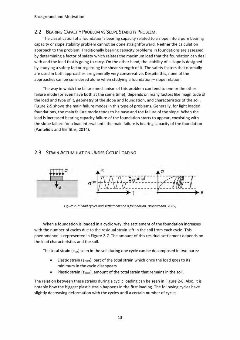
Figure 2-7: Load cycles and settlements on a foundation. (Wichtmann, 2005)
When a foundation is loaded in a cyclic way, the settlement of the foundation increases
with the number of cycles due to the residual strain left in the soil from each cycle. This
phenomenon is represented in Figure 2-7. The amount of this residual settlement depends on
the load characteristics and the soil.
The total strain (εtot) seen in the soil during one cycle can be decomposed in two parts:
• Elastic strain (εelast), part of the total strain which once the load goes to its
minimum in the cycle disappears.
• Plastic strain (εplast), amount of the total strain that remains in the soil.
The relation between these strains during a cyclic loading can be seen in Figure 2-8. Also, it is
notable how the biggest plastic strain happens in the first loading. The following cycles have
slightly decreasing deformation with the cycles until a certain number of cycles.

Background and Motivation
14
Figure 2-8: Representation of a strain history from a cyclic loading. (Adapted from Wichtmann, 2005)
Not every case behaves in the same way. Three main patterns can be defined according to
the plastic strain along the cycles (Goldscheider and Gudehus, 1976). In the case of stepwise
failure, the plastic strain that remains from each cycle is constant; in a shakedown case, the
remaining plastic strain reduces along the cycles until some point that only elastic
deformations occur; in an abation case the remaining plastic strain diminishes with the cycles
but never disappears completely.
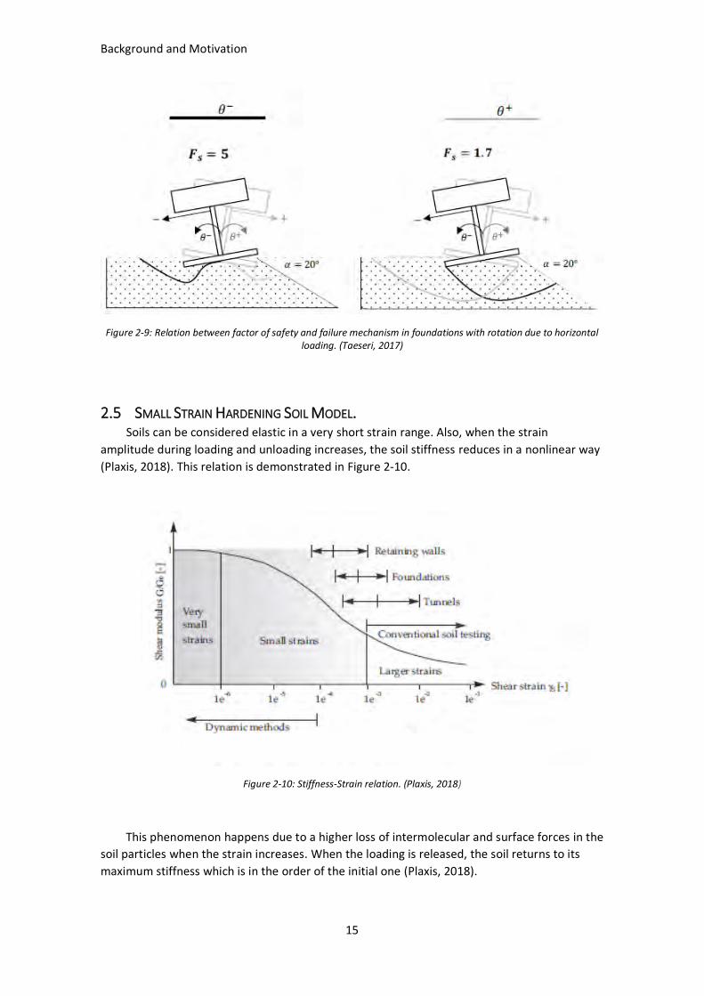
2.4 FAILURE BEHAVIOUR OF HORIZONTALLY LOADED FOUNDATIONS IN SLOPES When a foundation is affected by a horizontal load, rotation or sliding of it are common
occurrences. The amount of rotation depends on geometrical and soil parameters, also it is
strongly influenced by the load on the foundation and its horizontal-vertical ratio. The next
situations can occur for a surface foundation which suffers from important rotation. Figure 2-9
offers a clearer view of the phenomenon: (Taeseri, 2017)
• For big factors of safety (against vertical load), the failure surface is generated in the
same direction as the rotation.
• In case of safety factors close to 1 the failure is developed in the opposite direction as
the rotation.
This effect can also be noticed for embedded foundations, but this type is more resistant to
rotation than a foundation in the surface.
Background and Motivation
15
Figure 2-9: Relation between factor of safety and failure mechanism in foundations with rotation due to horizontal loading. (Taeseri, 2017)
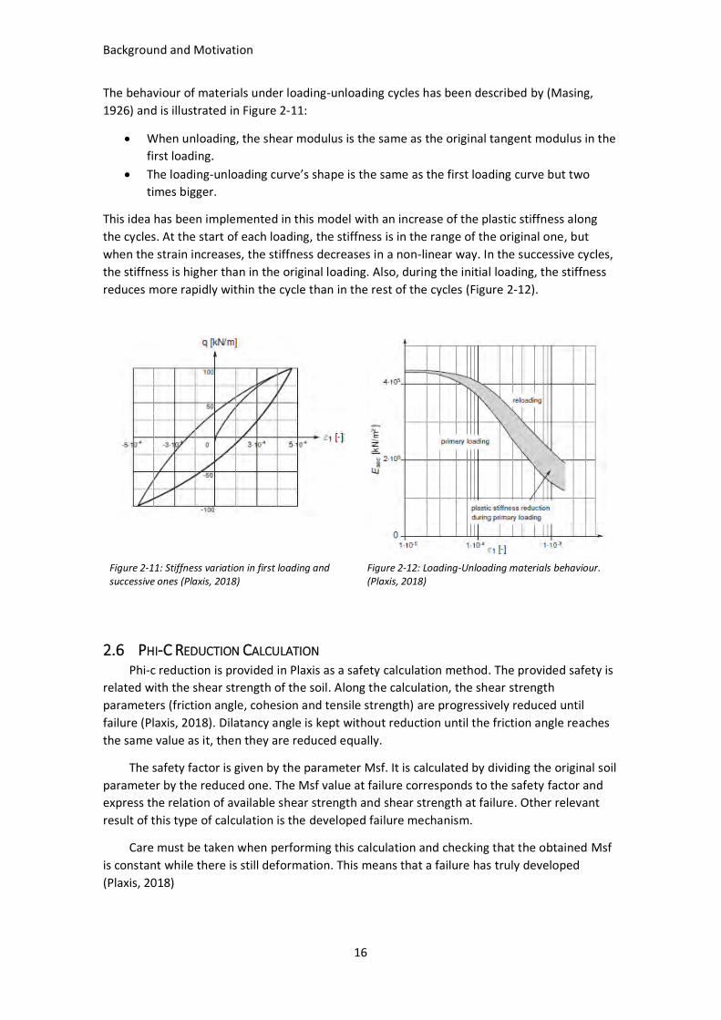
2.5 SMALL STRAIN HARDENING SOIL MODEL. Soils can be considered elastic in a very short strain range. Also, when the strain
amplitude during loading and unloading increases, the soil stiffness reduces in a nonlinear way
(Plaxis, 2018). This relation is demonstrated in Figure 2-10.
Figure 2-10: Stiffness-Strain relation. (Plaxis, 2018)
This phenomenon happens due to a higher loss of intermolecular and surface forces in the
soil particles when the strain increases. When the loading is released, the soil returns to its
maximum stiffness which is in the order of the initial one (Plaxis, 2018).
Background and Motivation
16
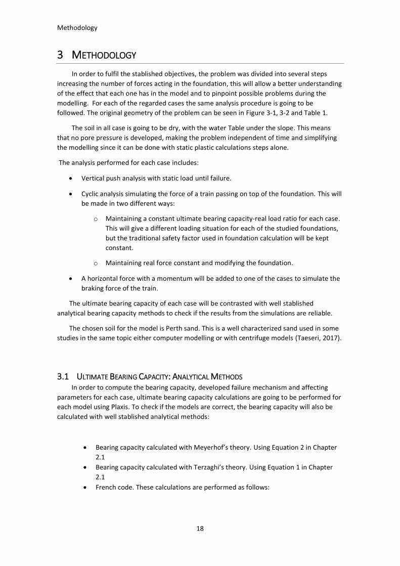
The behaviour of materials under loading-unloading cycles has been described by (Masing,
1926) and is illustrated in Figure 2-11:
• When unloading, the shear modulus is the same as the original tangent modulus in the
first loading.
• The loading-unloading curve’s shape is the same as the first loading curve but two
times bigger.
This idea has been implemented in this model with an increase of the plastic stiffness along
the cycles. At the start of each loading, the stiffness is in the range of the original one, but
when the strain increases, the stiffness decreases in a non-linear way. In the successive cycles,
the stiffness is higher than in the original loading. Also, during the initial loading, the stiffness
reduces more rapidly within the cycle than in the rest of the cycles (Figure 2-12).
Figure 2-11: Stiffness variation in first loading and successive ones (Plaxis, 2018)
Figure 2-12: Loading-Unloading materials behaviour. (Plaxis, 2018)
2.6 PHI-C REDUCTION CALCULATION Phi-c reduction is provided in Plaxis as a safety calculation method. The provided safety is
related with the shear strength of the soil. Along the calculation, the shear strength
parameters (friction angle, cohesion and tensile strength) are progressively reduced until
failure (Plaxis, 2018). Dilatancy angle is kept without reduction until the friction angle reaches
the same value as it, then they are reduced equally.
The safety factor is given by the parameter Msf. It is calculated by dividing the original soil
parameter by the reduced one. The Msf value at failure corresponds to the safety factor and
express the relation of available shear strength and shear strength at failure. Other relevant
result of this type of calculation is the developed failure mechanism.
Care must be taken when performing this calculation and checking that the obtained Msf
is constant while there is still deformation. This means that a failure has truly developed
(Plaxis, 2018)

Background and Motivation
17
2.7 AIM AND OBJECTIVES Two main cases are going to be regarded. A square foundation placed on top of the crest
of a slope and a foundation in the slope. In the second case, the slope is divided in two parts
with a small flat part in between where the foundation is placed. This can be normally seen in
real foundations due to the need of a working platform for the construction of it. These two
cases represent railway bridge foundations heavily loaded with the weight of the bridge and a
cyclic load corresponding to a train passing on top of them.
The principal aim of this work is to have a better understanding of the bearing behaviour
and failure mechanisms developed in foundations under the described conditions. The
stablished objectives are:
• Model foundations on slopes in Plaxis 2D.
• Analyse the ultimate bearing capacity of the different cases, the developed failure
mechanisms and understand some of the main parameters that influence the bearing
capacity.
• Study the bearing behaviour and how failures develop of the chosen cases under
several loading cycles.
• Find any difference, if it exists, between the failure mechanism present in a cyclic
loading and when a static bearing capacity failure happen.
Methodology
18
3 METHODOLOGY
In order to fulfil the stablished objectives, the problem was divided into several steps
increasing the number of forces acting in the foundation, this will allow a better understanding
of the effect that each one has in the model and to pinpoint possible problems during the
modelling. For each of the regarded cases the same analysis procedure is going to be
followed. The original geometry of the problem can be seen in Figure 3-1, 3-2 and Table 1.
The soil in all case is going to be dry, with the water Table under the slope. This means
that no pore pressure is developed, making the problem independent of time and simplifying
the modelling since it can be done with static plastic calculations steps alone.
The analysis performed for each case includes:
• Vertical push analysis with static load until failure.
• Cyclic analysis simulating the force of a train passing on top of the foundation. This will
be made in two different ways:
o Maintaining a constant ultimate bearing capacity-real load ratio for each case.
This will give a different loading situation for each of the studied foundations,
but the traditional safety factor used in foundation calculation will be kept
constant.
o Maintaining real force constant and modifying the foundation.
• A horizontal force with a momentum will be added to one of the cases to simulate the
braking force of the train.
The ultimate bearing capacity of each case will be contrasted with well stablished
analytical bearing capacity methods to check if the results from the simulations are reliable.
The chosen soil for the model is Perth sand. This is a well characterized sand used in some
studies in the same topic either computer modelling or with centrifuge models (Taeseri, 2017).
3.1 ULTIMATE BEARING CAPACITY: ANALYTICAL METHODS In order to compute the bearing capacity, developed failure mechanism and affecting
parameters for each case, ultimate bearing capacity calculations are going to be performed for
each model using Plaxis. To check if the models are correct, the bearing capacity will also be
calculated with well stablished analytical methods:
• Bearing capacity calculated with Meyerhof’s theory. Using Equation 2 in Chapter
2.1
• Bearing capacity calculated with Terzaghi’s theory. Using Equation 1 in Chapter
2.1
• French code. These calculations are performed as follows:
Methodology
19
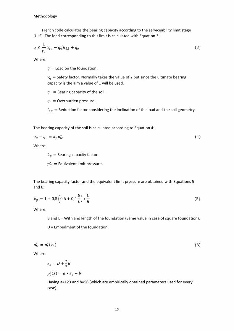
French code calculates the bearing capacity according to the serviceability limit stage
(ULS). The load corresponding to this limit is calculated with Equation 3:
𝑞 ≤1
𝛾𝑞
(𝑞𝑢 − 𝑞0)𝑖𝛿𝛽 + 𝑞𝑜 (3)
Where:
𝑞 = Load on the foundation.
𝛾𝑞 = Safety factor. Normally takes the value of 2 but since the ultimate bearing
capacity is the aim a value of 1 will be used.
𝑞𝑢 = Bearing capacity of the soil.
𝑞0 = Overburden pressure.
𝑖𝛿𝛽 = Reduction factor considering the inclination of the load and the soil geometry.
The bearing capacity of the soil is calculated according to Equation 4:
𝑞𝑢 − 𝑞0 = 𝑘𝑝𝑝𝑙𝑒∗ (4)
Where:
𝑘𝑝 = Bearing capacity factor.
𝑝𝑙𝑒∗ = Equivalent limit pressure.
The bearing capacity factor and the equivalent limit pressure are obtained with Equations 5
and 6:
𝑘𝑝 = 1 + 0,5 (0,6 + 0,4𝐵
𝐿) ∗
𝐷
𝐵 (5)
Where:
B and L = With and length of the foundation (Same value in case of square foundation).
D = Embedment of the foundation.
𝑝𝑙𝑒∗ = 𝑝𝑙
∗(𝑧𝑒) (6)
Where:
𝑧𝑒 = 𝐷 +2
3𝐵
𝑝𝑙∗(𝑧) = 𝑎 ∗ 𝑧𝑒 + 𝑏
Having a=123 and b=56 (which are empirically obtained parameters used for every
case).

Methodology
20
Finally, the reduction factor is computed with Equation 7:
𝑖𝛿𝛽 = 1 − 0,9 tan(𝛽) (2 − tan(𝛽)) [max ((1 −𝑑
8𝐵) ; 0)]
2
(7)
Where:
𝛽 = Inclination of the slope.
d = Distance from the foundation to the edge of the crest.
3.2 PLAXIS MODELS As two geometries are regarded, two basic models are developed. These models will be
the base on where further modifications will be made.
The foundation studied in the bearing capacity calculations and in the constant force ratio
is a square foundation with the characteristic shown in Table 1. For the real force calculations,
the geometry of the foundation will be modified to fit the load requirements. The geometry
from Table 1 is based on foundations studied in centrifuge tests in Taeseri, 2017.
Table 1: Original geometry of the foundation.
Side Length Thickness Embedment Ration Material
B= 2,8 m D=1,12 m 0,4 Aluminium
In the mentioned study made by Taeseri, Aluminium is chosen as the foundation’s
material in the physical models for having a similar density to concrete, which will be also
followed here. Also, the foundation will be made fairly rigid. The point of this study is to
analyse the interaction between the soil and the foundation and not the structural behaviour
of the foundation.
Figure 3-1 and Figure 3-2 show the original geometry of the complete model for both
studied cases. The original model is made with a slope of 20º angle. In order to study the effect
of the slope angle in the foundation, a 30º angle slope will also be modelled. For consistency,
the height of the slope is 8 m in every case.
The chosen size for the model is 40 x 20 m, being big enough to avoid boundary effects in
the models. More information about how the boundaries were set can be found in Appendix
III.
Methodology
21
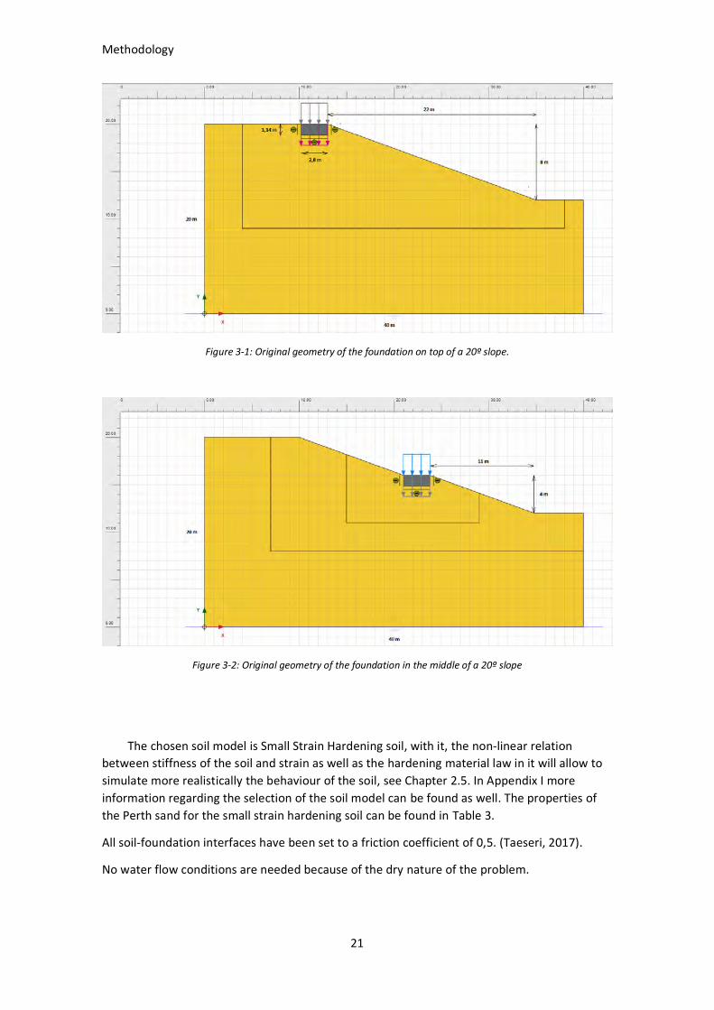
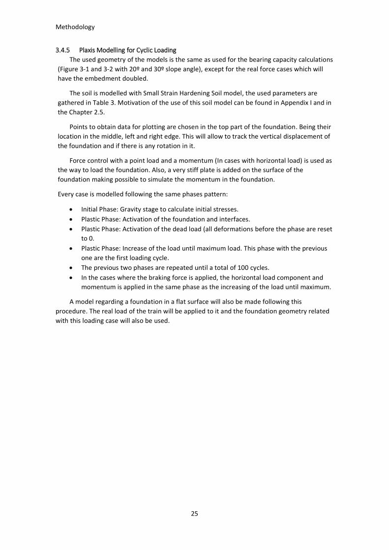
Figure 3-1: Original geometry of the foundation on top of a 20º slope.
Figure 3-2: Original geometry of the foundation in the middle of a 20º slope
The chosen soil model is Small Strain Hardening soil, with it, the non-linear relation
between stiffness of the soil and strain as well as the hardening material law in it will allow to
simulate more realistically the behaviour of the soil, see Chapter 2.5. In Appendix I more
information regarding the selection of the soil model can be found as well. The properties of
the Perth sand for the small strain hardening soil can be found in Table 3.
All soil-foundation interfaces have been set to a friction coefficient of 0,5. (Taeseri, 2017).
No water flow conditions are needed because of the dry nature of the problem.

Methodology
22
3.3 ULTIMATE BEARING CAPACITY PLAXIS For calculating the ultimate bearing capacity of the foundation, the way Plaxis applies a
load during a plastic phase is going to be used. This load is not applied at once, it goes
gradually increasing with the iterations until it reaches the defined value or the soil collapses.
The amount of the applied load during the calculations is denoted by the program with the
Mstage parameter. This parameter ranges from 0 to 1, being 0 equal to no applied load and 1
the total of the designated load is applied. As an example, if a load of -100 kN/m/m is
designated, the Mstage will be 0,5 when -50 kN/m/m are applied in the calculations.
The way to find the ultimate bearing capacity is: first an arbitrary big load is placed in the
foundation, which makes the soil body collapse since is bigger than the bearing capacity. At
this point, the reached Mstage is checked and multiplied by the applied load. The result is the
maximum load that could be applied before collapse or, in other words the ultimate bearing
capacity. Finally, the model is calculated once again with the calculated load. Doing this the
load is checked and the failure mechanism can be observed in the results.
The calculated models are the ones with the original geometry shown in Figure 3-1 and 3-
2 with a slope angle of 20º and 30º. Also, the same models are calculated once again with the
embedment of the foundation doubled.
Several mesh sizes were tried until the adequate one was found. The selected one is a bit
finer than the minimum required, since the calculation time in these models is not a problem.
Also, this mesh provides good quality.
The stages used to calculate these models are:
• Initial phase where the initial stresses are computed. This is done only with gravity
loading since there is no phreatic in the model.
• During the second phase, the foundation is placed in the soil and the interfaces
activated. After this stage all displacement are reset.
• In the next phase the force is activated.
• Two more phases are added with halve and 2/3 of the ultimate bearing capacity.
3.4 CYCLIC LOADING MODELS When a train passes on top of a foundation, the loads generated by it can be divided into
three steps. Initially the train starts entering the influence area of the foundation increasing
the vertical load on it. Once the head of the train has passed the foundation and left the
influence area, the load stops increasing and stays stable until the end of the train enters the
influence area. At this point the load starts decreasing until the end of the trains lives the
influence area when the train load becomes zero again.
3.4.1 Calculation of Vertical Train Load
For calculating the loads related with a train passing on top of the foundation, several
assumptions and simplifications are made:

Methodology
23
• The bridge that the foundation supports has 30m span, being the smallest span where the
inertia of moving vehicles can be neglected (Unsworth, 2017). Also, the dead load of the
bridge is assumed to be 96 tons (being a reasonable load for a bridge of medium size
(Taeseri, 2017) which gives a force of 940 kN or a dead load of 336 kN/m (as a point load
in Plaxis 2D the units are kN/m).
• The wagons of the passing train have a weight of 30 tons (no difference made between
wagons and locomotive) with a length of 9,4 m. This leads to a line load of 31,3 kN/m. The
speed of the train is chosen to be 30 km/h (8,33 m/s). With very long trains, the interval
when the load is constant at its maximum is also long. This is important in cases when
pore pressure can develop, although this fact is not applicable for this case.
• All the generated loads will be transferred to a point load in the middle of the foundation.
The load is assumed to affect the foundation from the half of the spam before and after the
foundation (15 m on each side of the foundation). In this way, the line load of the train is
calculated as a moving point load with increasing value until the train is covering the full
influence length. The same calculations are made when the train leaves the influence length of
the bridge. In Figure 3-3 the profile of the calculated load can be seen.
Figure 3-3: Load profile on the foundation generated by a train passing on top, according to the assumptions and simplifications made.
The maximum reached force is 939 kN, which transferred to a point load in the foundation
gives 335 kN/m. The calculated loads that are going to be applied are summarised in Table 2.
From now on these loads are going to be referred as real loads
Table 2: Real loads applied on the foundation.
Dead Load [kN/m] Train Load [kN/m] Maximum Load [kN/m]
336 335 671
Each load corresponds to the 50 % of the maximum one.
0
100
200
300
400
500
600
700
800
900
1000
0 5 10 15 20 25 30
Load
[kN
]
time [s]
Train Load

Methodology
24
3.4.2 Calculation of Horizontal Train Load
The horizontal forces in the bridge are generated by the movement of trains along the
bridge. These horizontal forces are transferred to the tracks by friction forces between wheels
and tracks, and from the tracks to the superstructure and substructure of the bridge. The
horizontal forces generated by the train moving at constant speed are small, but they reach
bigger values when the train brakes or accelerates (Fryba, 1996).
Traditionally this force does not play an important role when designing a foundation for a
small or medium bridge. In these cases, it is considered that this force act only in the
abutments and any horizontal load in the foundations is just covered by the conservative
safety factors used for its design. But even being small, this force generates a cyclic loading in
the foundation that can affect the bearing capacity in a long term.
The horizontal force generated by a train braking is taken as 25% of the axle load (Chen
and Duan, 2000). According to this and having a wagon with 30 tons weight and four axles,
each axle deals with a load of 73,5 kN. Giving a braking force of 18,375 kN. Which transferred
to a point load in Plaxis is 6,56 kN/m.
Since this load is applied on the bridge it will be transferred to the foundation by a
horizontal component to the load of 6,56 kN/m and a momentum. This momentum is
calculated according to the height of the pier that connects the foundation with the bridge,
this height is assumed to be 4m (Taeseri, 2017). For this situation the momentum is 26,25
kN·m/m. The momentum will be applied in a clockwise direction with a horizontal force
pointing right to simulate a train passing through the bridge from left to right. The opposite
force and momentum will be applied to simulate a train going from right to left.
3.4.3 Constant Force Ratio Loading
For this situation, all cases have a ratio between bearing capacity and applied load of 3,7
(Equation 8). This can also be seen as a traditional safety factor of 3,7 (A value between 3 and
4 is commonly used for design of foundations). The ratio between dead load and maximum
train load is also maintained, corresponding 50% of the total load to the dead load and 50% to
the maximum train load. The calculated loads that are going to be applied can be found in
Table 6.
𝑈𝑙𝑡𝑖𝑚𝑎𝑡𝑒 𝐵𝑒𝑎𝑟𝑖𝑛𝑔 𝐶𝑎𝑝𝑎𝑐𝑖𝑡𝑦
𝐴𝑝𝑝𝑙𝑖𝑒𝑑 𝑀𝑎𝑥𝑖𝑚𝑢𝑚 𝐿𝑜𝑎𝑑= 3,7 (8)
3.4.4 Real Force Loading
The real load is too big for the original foundation’s geometry. In real situations with this
kind of foundations it is common to have a limited building area so increasing the area of the
foundation is not an option. The common solution is to increase the depth of embedment.
Following this praxis, the embedment of the foundation will be doubled, being the new one
2,24 m.
The applied load for every case can be found in Table 2.
Methodology
25
3.4.5 Plaxis Modelling for Cyclic Loading
The used geometry of the models is the same as used for the bearing capacity calculations
(Figure 3-1 and 3-2 with 20º and 30º slope angle), except for the real force cases which will
have the embedment doubled.
The soil is modelled with Small Strain Hardening Soil model, the used parameters are
gathered in Table 3. Motivation of the use of this soil model can be found in Appendix I and in
the Chapter 2.5.
Points to obtain data for plotting are chosen in the top part of the foundation. Being their
location in the middle, left and right edge. This will allow to track the vertical displacement of
the foundation and if there is any rotation in it.
Force control with a point load and a momentum (In cases with horizontal load) is used as
the way to load the foundation. Also, a very stiff plate is added on the surface of the
foundation making possible to simulate the momentum in the foundation.
Every case is modelled following the same phases pattern:
• Initial Phase: Gravity stage to calculate initial stresses.
• Plastic Phase: Activation of the foundation and interfaces.
• Plastic Phase: Activation of the dead load (all deformations before the phase are reset
to 0.
• Plastic Phase: Increase of the load until maximum load. This phase with the previous
one are the first loading cycle.
• The previous two phases are repeated until a total of 100 cycles.
• In the cases where the braking force is applied, the horizontal load component and
momentum is applied in the same phase as the increasing of the load until maximum.
A model regarding a foundation in a flat surface will also be made following this
procedure. The real load of the train will be applied to it and the foundation geometry related
with this loading case will also be used.

Results and Analysis
26
4 RESULTS AND ANALYSIS
4.1 ULTIMATE BEARING CAPACITY
4.1.1 Input
The soil parameters of the Perth sand used in the Small Strain Hardening Soil for the computer
calculations are gathered in Table 3.
Table 3: Perth sand parameters for Small Strain Hardening Soil model
Parameters Perth Sand
Effective particle size, 𝐷10 (𝑚𝑚) 0.14
Average particle size, 𝐷50 (𝑚𝑚) 0.23
Uniformity coefficient, 𝐶𝑢 1.79
Coefficient of curvature, 𝐶𝑐 1.26
Specific density, 𝜌𝑠 (𝑘𝑔/𝑚3) 2700
Dry density, 𝜌𝑑 (𝑘𝑔/𝑚3) 1700
Relative density, 𝐷𝑟 (%) 80
Void ratio, 𝑒𝑚𝑖𝑛 … 𝑒𝑚𝑎𝑥 0.502…0.752
Friction angle, 𝜑′𝑚𝑎𝑥(°) 38
Dilatancy angle, 𝜓 (°) 8
Surface shear modulus, 𝐺0 (𝑘𝑃𝑎) 35000
Surface shear wave velocity 𝑉𝑠,0 (𝑚/𝑠) 150
Secant stiffness, 𝐸50𝑟𝑒𝑓(𝑘𝑃𝑎) 33000
Tangent stiffness, 𝐸𝑜𝑒𝑑𝑟𝑒𝑓 (𝑘𝑃𝑎) 27150
Unloading reloading stiffness, 𝐸𝑢𝑟𝑟𝑒𝑓 (𝑘𝑃𝑎) 99000
Shear strain, 𝛾0.72 (−) 2x10⁻⁴
Shear modulus at very small strains, 𝐺0𝑟𝑒𝑓 (𝑘𝑃𝑎) 190000
Reference stress level, 𝑃𝑟𝑒𝑓 (𝑘𝑃𝑎) 100
In the case of the hand calculations, dry density is used from Table 3, a friction angle of 30º
(which comes from the subtraction of the dilatancy, 8º; to the real friction angle 38º), and the
specific parameters needed in each case are obtained from the Figures presented in Chapter
2.1
4.1.2 Calculations
Analytical calculations are made with the formulas related with each of the three methods
presented in Chapters 2.1 and 3.1
The Plaxis models are calculated following the stages from Chapter 3.3.

Results and Analysis
27
4.1.3 Output
4.1.3.1 Analytical Calculations
Table 4 gathers the ultimate bearing capacity obtained from the three analytical methods
for each case. Terzaghi and French Code methods are only applied for the cases with the
foundation on top of the slope.
Table 4: Ultimate bearing capacity results from the three analytical calculations
Case Meyerhof Terzaghi French Code
Top, 20º slope 671,73 kN/m2 552,04 kN/m2 527,184 kN/m2
Top, 30º slope 480,47 kN/m2 268,46 kN/m2 151,38 kN/m2
Middle, 20º slope 848,99 kN/m2 - -
Middle, 30º slope 587,76 kN/m2 - -
4.1.3.2 Original Geometry Cases
A) FOUNDATION ON TOP OF A 20º ANGLE SLOPE, ORIGINAL GEOMETRY
The following set of figures shows the incremental displacements and incremental
deviatoric strain generated by the ultimate load (Mstage = 1). Vertical displacement- load
curve is also included.
Figure 4-1: Incremental displacements plot from ultimate bearing capacity calculations of a foundation on top of a 20º slope
Results and Analysis
28
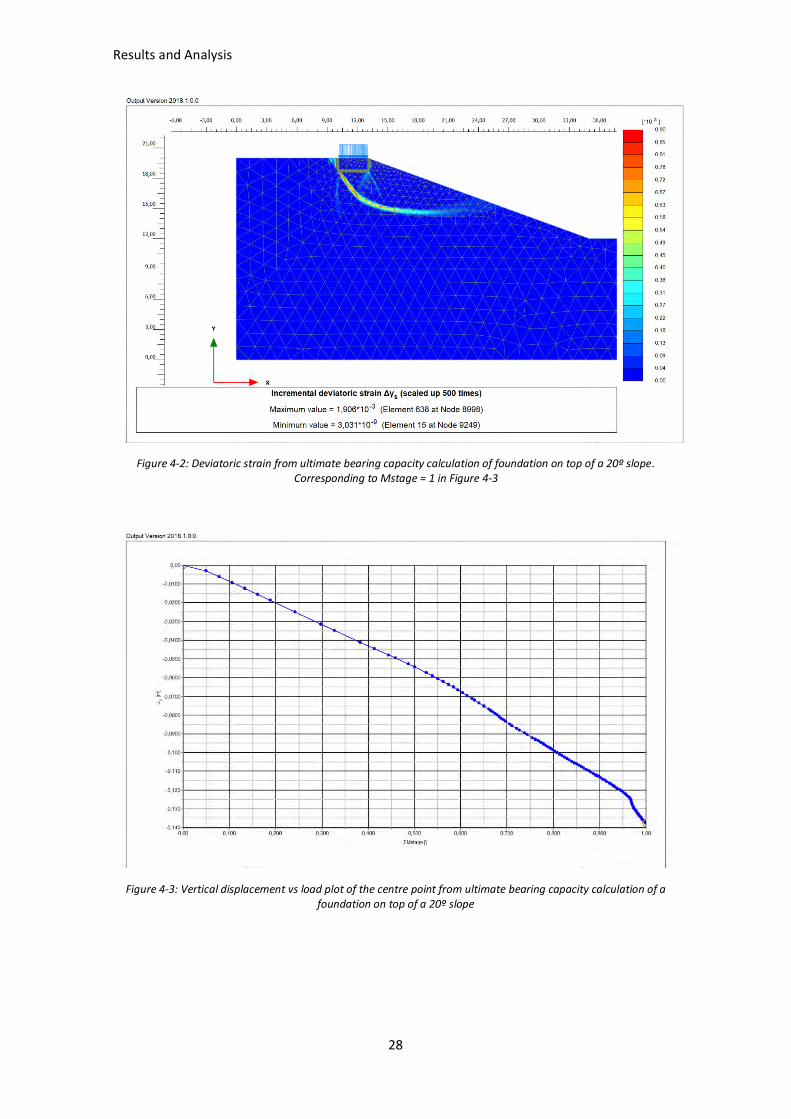
Figure 4-2: Deviatoric strain from ultimate bearing capacity calculation of foundation on top of a 20º slope. Corresponding to Mstage = 1 in Figure 4-3
Figure 4-3: Vertical displacement vs load plot of the centre point from ultimate bearing capacity calculation of a foundation on top of a 20º slope
Results and Analysis
29
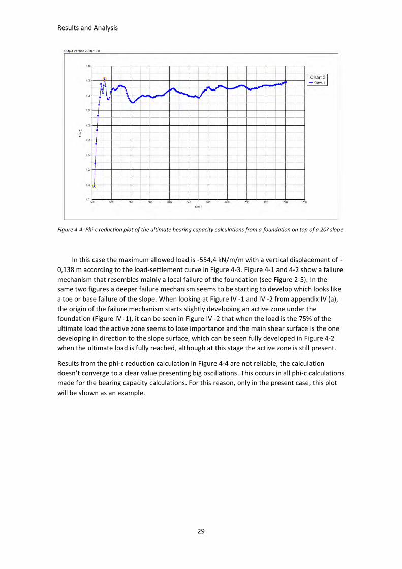
Figure 4-4: Phi-c reduction plot of the ultimate bearing capacity calculations from a foundation on top of a 20º slope
In this case the maximum allowed load is -554,4 kN/m/m with a vertical displacement of -
0,138 m according to the load-settlement curve in Figure 4-3. Figure 4-1 and 4-2 show a failure
mechanism that resembles mainly a local failure of the foundation (see Figure 2-5). In the
same two figures a deeper failure mechanism seems to be starting to develop which looks like
a toe or base failure of the slope. When looking at Figure IV -1 and IV -2 from appendix IV (a),
the origin of the failure mechanism starts slightly developing an active zone under the
foundation (Figure IV -1), it can be seen in Figure IV -2 that when the load is the 75% of the
ultimate load the active zone seems to lose importance and the main shear surface is the one
developing in direction to the slope surface, which can be seen fully developed in Figure 4-2
when the ultimate load is fully reached, although at this stage the active zone is still present.
Results from the phi-c reduction calculation in Figure 4-4 are not reliable, the calculation
doesn’t converge to a clear value presenting big oscillations. This occurs in all phi-c calculations
made for the bearing capacity calculations. For this reason, only in the present case, this plot
will be shown as an example.
Results and Analysis
30
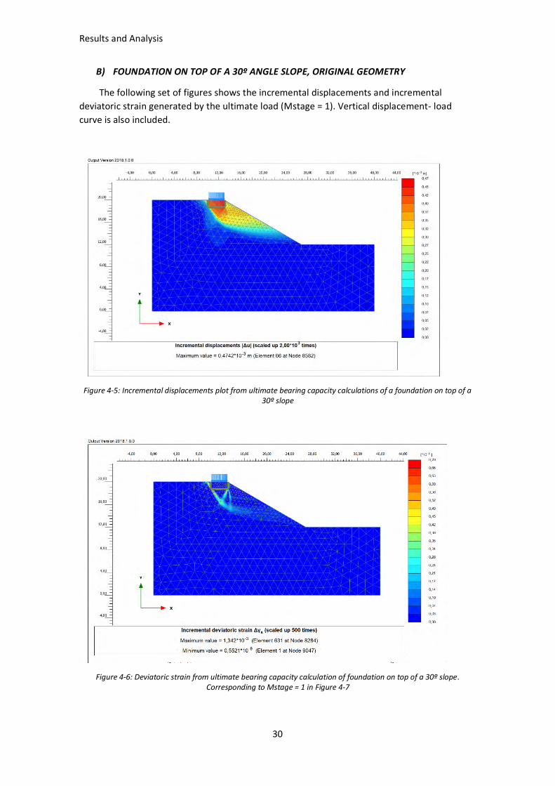
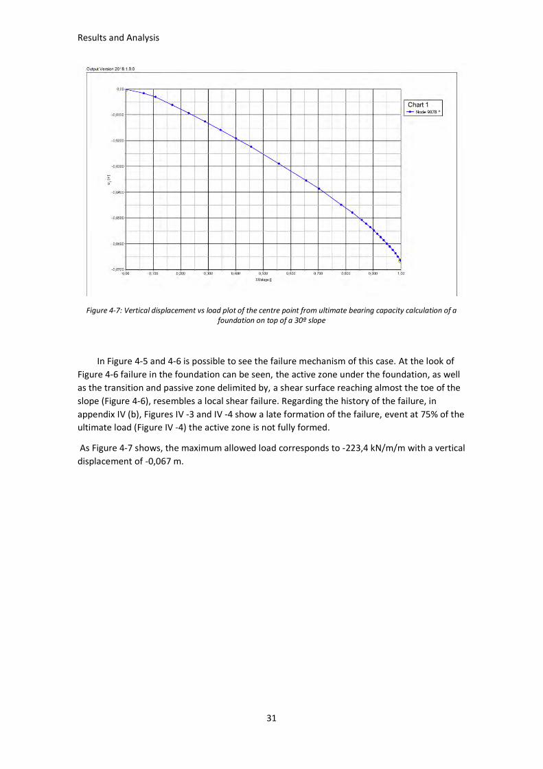
B) FOUNDATION ON TOP OF A 30º ANGLE SLOPE, ORIGINAL GEOMETRY
The following set of figures shows the incremental displacements and incremental
deviatoric strain generated by the ultimate load (Mstage = 1). Vertical displacement- load
curve is also included.
Figure 4-5: Incremental displacements plot from ultimate bearing capacity calculations of a foundation on top of a 30º slope
Figure 4-6: Deviatoric strain from ultimate bearing capacity calculation of foundation on top of a 30º slope. Corresponding to Mstage = 1 in Figure 4-7
Results and Analysis
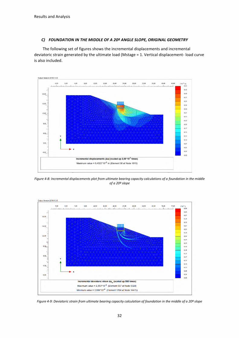
31
Figure 4-7: Vertical displacement vs load plot of the centre point from ultimate bearing capacity calculation of a foundation on top of a 30º slope
In Figure 4-5 and 4-6 is possible to see the failure mechanism of this case. At the look of
Figure 4-6 failure in the foundation can be seen, the active zone under the foundation, as well
as the transition and passive zone delimited by, a shear surface reaching almost the toe of the
slope (Figure 4-6), resembles a local shear failure. Regarding the history of the failure, in
appendix IV (b), Figures IV -3 and IV -4 show a late formation of the failure, event at 75% of the
ultimate load (Figure IV -4) the active zone is not fully formed.
As Figure 4-7 shows, the maximum allowed load corresponds to -223,4 kN/m/m with a vertical
displacement of -0,067 m.
Results and Analysis
32
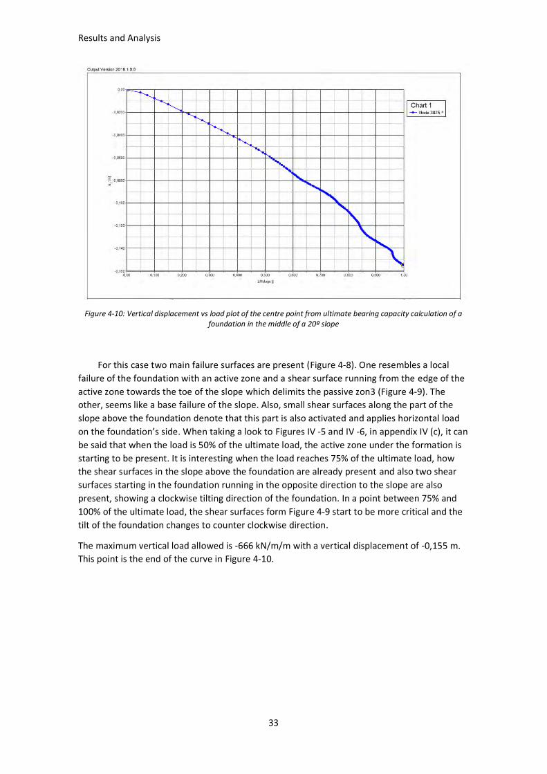
C) FOUNDATION IN THE MIDDLE OF A 20º ANGLE SLOPE, ORIGINAL GEOMETRY
The following set of figures shows the incremental displacements and incremental
deviatoric strain generated by the ultimate load (Mstage = 1. Vertical displacement- load curve
is also included.
Figure 4-8: Incremental displacements plot from ultimate bearing capacity calculations of a foundation in the middle of a 20º slope
Figure 4-9: Deviatoric strain from ultimate bearing capacity calculation of foundation in the middle of a 20º slope
Results and Analysis
33
Figure 4-10: Vertical displacement vs load plot of the centre point from ultimate bearing capacity calculation of a foundation in the middle of a 20º slope
For this case two main failure surfaces are present (Figure 4-8). One resembles a local
failure of the foundation with an active zone and a shear surface running from the edge of the
active zone towards the toe of the slope which delimits the passive zon3 (Figure 4-9). The
other, seems like a base failure of the slope. Also, small shear surfaces along the part of the
slope above the foundation denote that this part is also activated and applies horizontal load
on the foundation’s side. When taking a look to Figures IV -5 and IV -6, in appendix IV (c), it can
be said that when the load is 50% of the ultimate load, the active zone under the formation is
starting to be present. It is interesting when the load reaches 75% of the ultimate load, how
the shear surfaces in the slope above the foundation are already present and also two shear
surfaces starting in the foundation running in the opposite direction to the slope are also
present, showing a clockwise tilting direction of the foundation. In a point between 75% and
100% of the ultimate load, the shear surfaces form Figure 4-9 start to be more critical and the
tilt of the foundation changes to counter clockwise direction.
The maximum vertical load allowed is -666 kN/m/m with a vertical displacement of -0,155 m.
This point is the end of the curve in Figure 4-10.
Results and Analysis
34
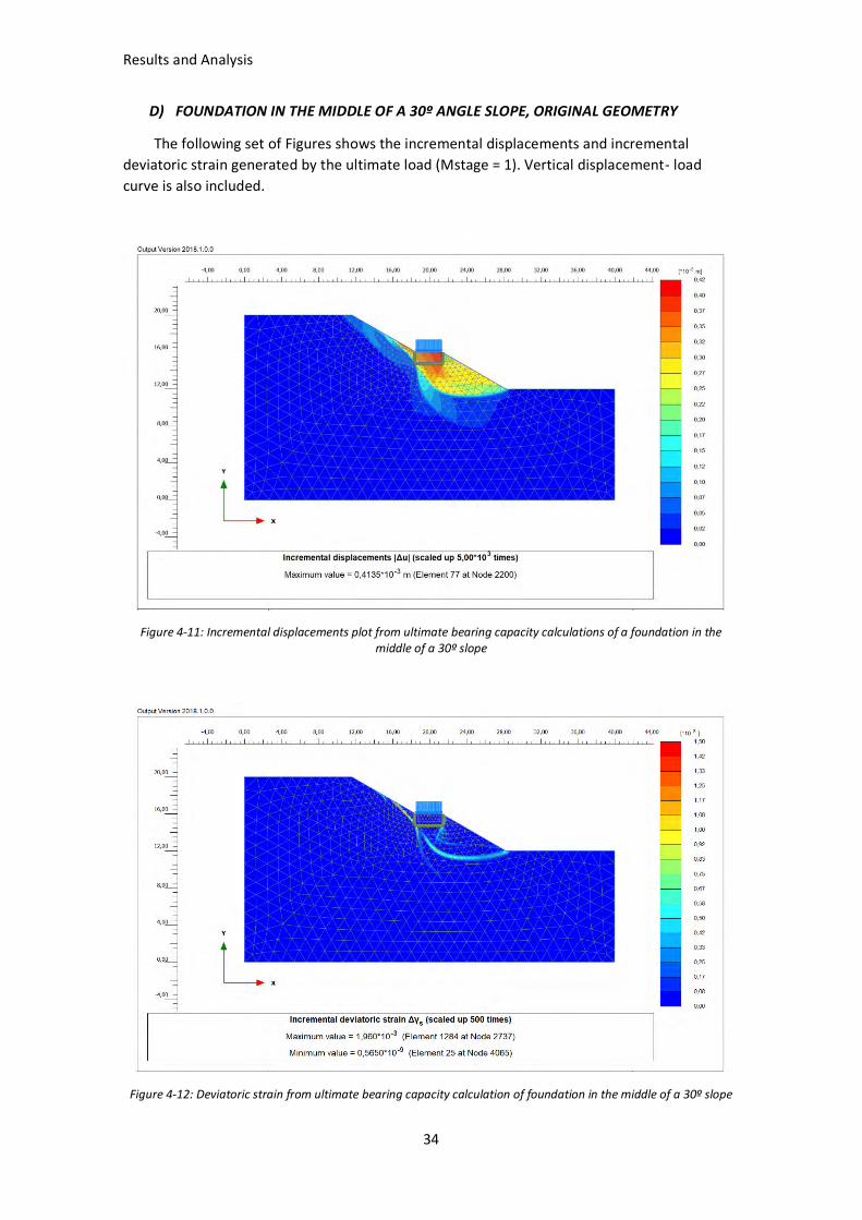
D) FOUNDATION IN THE MIDDLE OF A 30º ANGLE SLOPE, ORIGINAL GEOMETRY
The following set of Figures shows the incremental displacements and incremental
deviatoric strain generated by the ultimate load (Mstage = 1). Vertical displacement- load
curve is also included.
Figure 4-11: Incremental displacements plot from ultimate bearing capacity calculations of a foundation in the middle of a 30º slope
Figure 4-12: Deviatoric strain from ultimate bearing capacity calculation of foundation in the middle of a 30º slope

Results and Analysis
35
Figure 4-13: Vertical displacement vs load plot of the centre point from ultimate bearing capacity calculation of a foundation in the middle of a 30º slope
As seen in Figure 4-11 and 4-12, there is a foundation failure with a fully developed active
zone under the foundation and a shear surface running from this zone until the toe of the
slope. The start of a deeper failure surface in the slope is also visible (Figure 4-11 and 4-12).
The shear surface showing the biggest amount of strain is the one located in the slope above
the foundation (Figure 4-12). When looking at Figures IV -7 and IV -8 from appendix IV (d), it
can be said that the development of the shear surfaces is quite late, when the 50% of the
ultimate load the active zone is not fully developed (Figure IV -7), and when the 75% of the
load is applied the active zone is present as well as the shear surface from the active zone
towards the toe of the foundation and the shear surface in the part of the slope above the
foundation (Figure IV -8).
The maximum load obtained from the end point of Figure 4-13 is -423,5 kN/m/m with a
vertical displacement of -0,118 m.
Results and Analysis
36
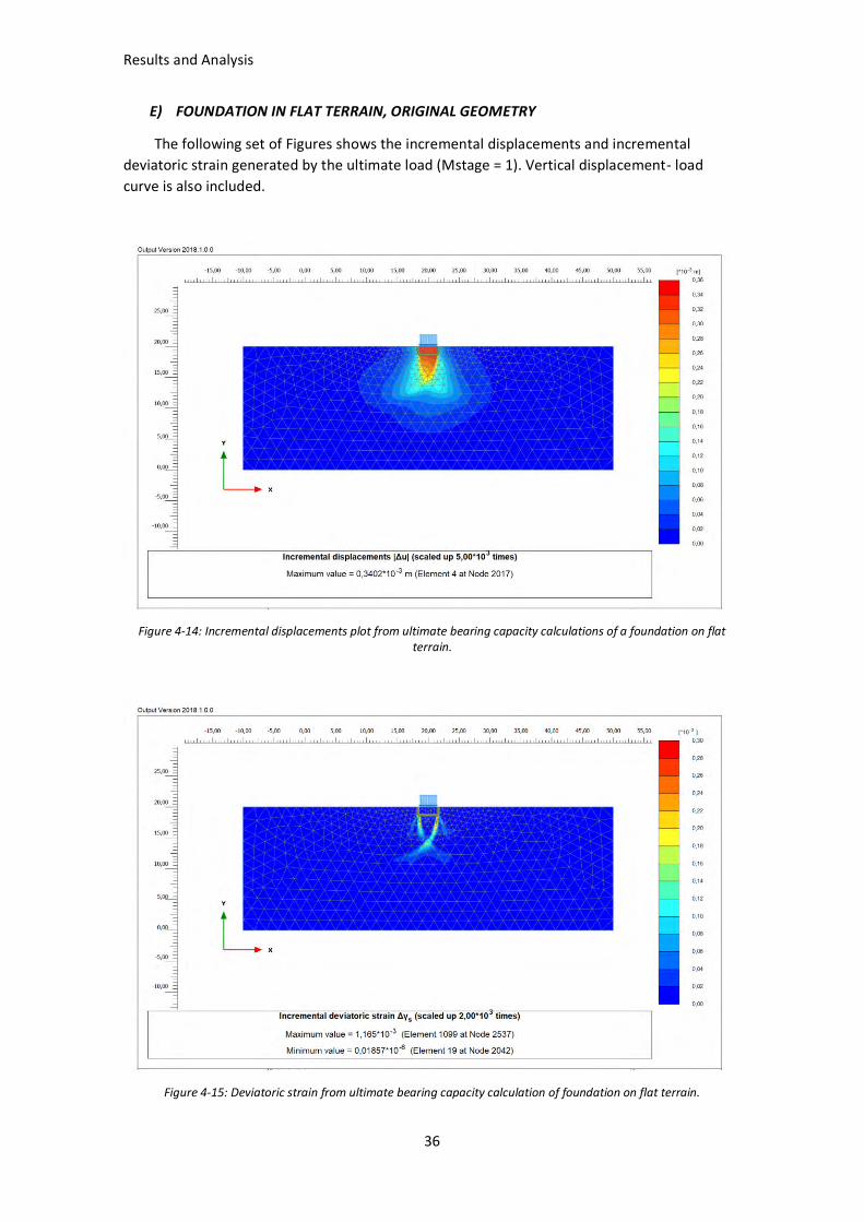
E) FOUNDATION IN FLAT TERRAIN, ORIGINAL GEOMETRY
The following set of Figures shows the incremental displacements and incremental
deviatoric strain generated by the ultimate load (Mstage = 1). Vertical displacement- load
curve is also included.
Figure 4-14: Incremental displacements plot from ultimate bearing capacity calculations of a foundation on flat terrain.
Figure 4-15: Deviatoric strain from ultimate bearing capacity calculation of foundation on flat terrain.
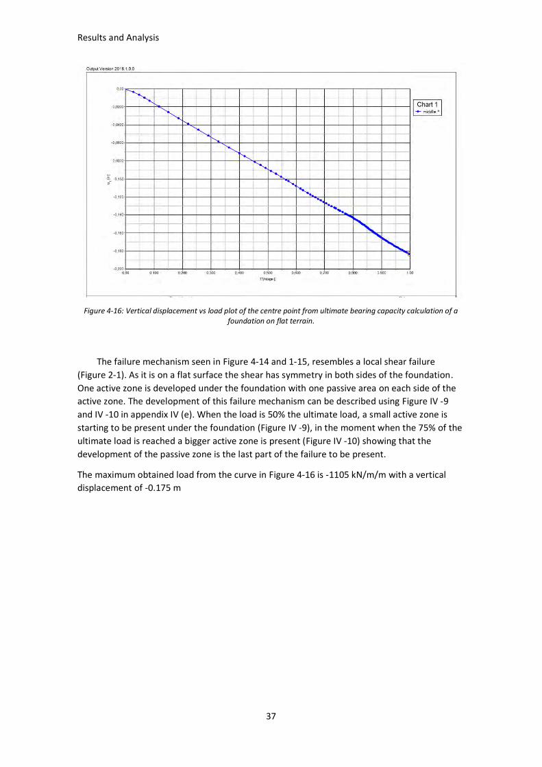
Results and Analysis
37
Figure 4-16: Vertical displacement vs load plot of the centre point from ultimate bearing capacity calculation of a foundation on flat terrain.
The failure mechanism seen in Figure 4-14 and 1-15, resembles a local shear failure
(Figure 2-1). As it is on a flat surface the shear has symmetry in both sides of the foundation.
One active zone is developed under the foundation with one passive area on each side of the
active zone. The development of this failure mechanism can be described using Figure IV -9
and IV -10 in appendix IV (e). When the load is 50% the ultimate load, a small active zone is
starting to be present under the foundation (Figure IV -9), in the moment when the 75% of the
ultimate load is reached a bigger active zone is present (Figure IV -10) showing that the
development of the passive zone is the last part of the failure to be present.
The maximum obtained load from the curve in Figure 4-16 is -1105 kN/m/m with a vertical
displacement of -0.175 m
Results and Analysis
38
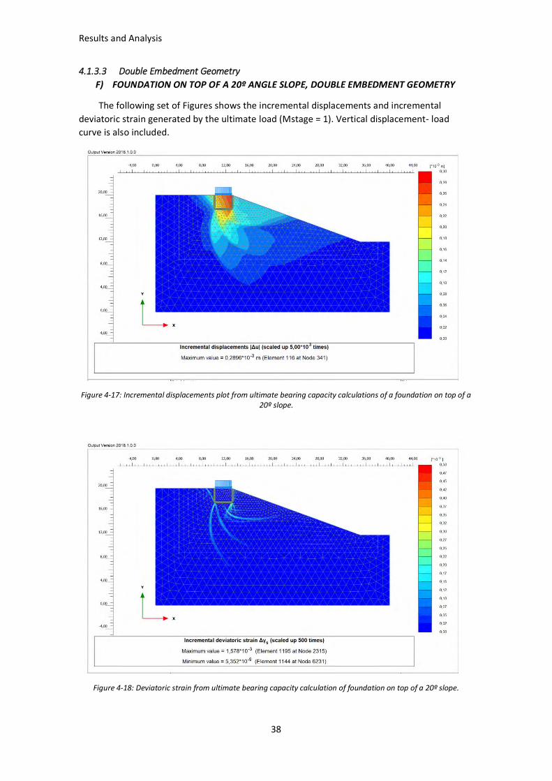
4.1.3.3 Double Embedment Geometry
F) FOUNDATION ON TOP OF A 20º ANGLE SLOPE, DOUBLE EMBEDMENT GEOMETRY
The following set of Figures shows the incremental displacements and incremental
deviatoric strain generated by the ultimate load (Mstage = 1). Vertical displacement- load
curve is also included.
Figure 4-17: Incremental displacements plot from ultimate bearing capacity calculations of a foundation on top of a 20º slope.
Figure 4-18: Deviatoric strain from ultimate bearing capacity calculation of foundation on top of a 20º slope.

Results and Analysis
39
Figure 4-19: Vertical displacement vs load plot of the centre point from ultimate bearing capacity calculation of a foundation on top of a 20º slope.
Figure 4-17 and 4-18 show three main failure mechanism toward the slope, one starting
from the active zone under the foundation that seems to go towards the toe of the
foundation, a deeper shear surface resembling the start of a base failure and one shallower.
Also, in the left side of the foundation one shear surface is present form the bottom left corner
of the foundation to the surface (also looks like it has the same direction as the shallower
shear surface on the right. At the look of Figure IV -11 and IV -12 (appendix IV, (f)), when the
50% of the ultimate load is applied, the active zone under the foundation is present (Figure IV -
11), the moment the load reaches the 75% of the ultimate load, an active zone under the
foundation and what seems a passive zone at each side of the active is visible, one of the shear
surfaces is already getting close to the slope surface (it seems to be the shallower shear
surface in the ultimate stage of the failure).
The ultimate reached load is -871,3 kN/m/m with a vertical displacement of -0,176 m, from
Figure 4-19.
Results and Analysis
40
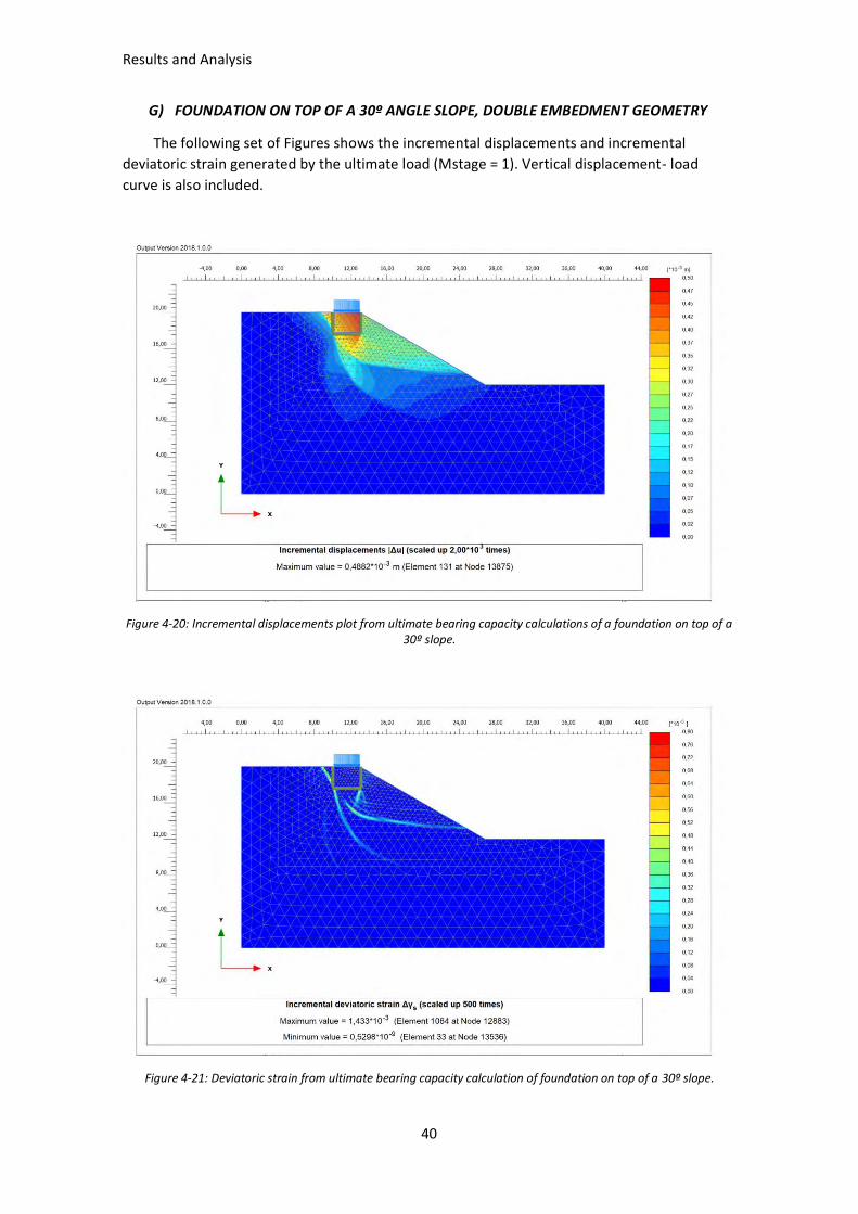
G) FOUNDATION ON TOP OF A 30º ANGLE SLOPE, DOUBLE EMBEDMENT GEOMETRY
The following set of Figures shows the incremental displacements and incremental
deviatoric strain generated by the ultimate load (Mstage = 1). Vertical displacement- load
curve is also included.
Figure 4-20: Incremental displacements plot from ultimate bearing capacity calculations of a foundation on top of a 30º slope.
Figure 4-21: Deviatoric strain from ultimate bearing capacity calculation of foundation on top of a 30º slope.

Results and Analysis
41
Figure 4-22: Vertical displacement vs load plot of the centre point from ultimate bearing capacity calculation of a foundation on top of a 30º slope.
Figure 4-21 and 4-20 show a similar mechanism than in the 20º case but shallower, the
main shear surface that goes until the slope surface seems to cut the active zone and has the
same direction as the failure surface on the left of the foundation. A deeper shear surface
starting from the active zone is also present, as well as the start of what it seems a base failure.
From Figures IV -13 and IV -14 in appendix IV (g), when the load is 50% of the ultimate load,
the active zone is already present, in this point the shear surface from the active zone to the
surface of the slope is starting to develop. This shear surface seems to move deeper and reach
the horizontal surface on the left of the foundation when the applied load reaches 70% of the
ultimate load, the start of what seems a base failure is also present, but it does not present big
strains.
From Figure 4-22, the ultimate reached load is -445,2 kN/m/m with a vertical displacement of -
0,111 m.

Results and Analysis
42
H) FOUNDATION IN THE MIDDLE OF A 20º ANGLE SLOPE, DOUBLE EMBEDMENT
GEOMETRY
The following set of Figures shows the incremental displacements and incremental
deviatoric strain generated by the ultimate load (Mstage = 1). Vertical displacement- load
curve is also included.
Figure 4-23: Incremental displacements plot from ultimate bearing capacity calculations of a foundation in the middle of a 20º slope.
Figure 4-24: Deviatoric strain from ultimate bearing capacity calculation of foundation in the middle of a 20º slope.
Results and Analysis
43
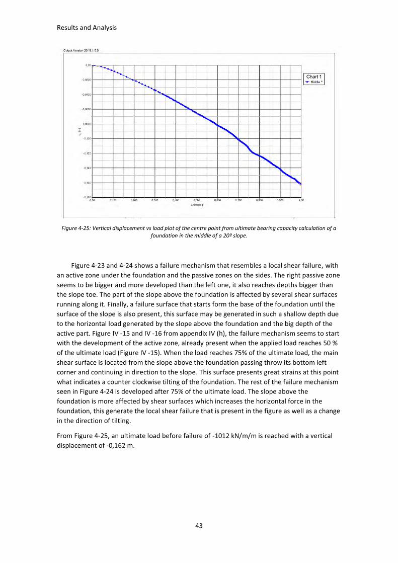
Figure 4-25: Vertical displacement vs load plot of the centre point from ultimate bearing capacity calculation of a foundation in the middle of a 20º slope.
Figure 4-23 and 4-24 shows a failure mechanism that resembles a local shear failure, with
an active zone under the foundation and the passive zones on the sides. The right passive zone
seems to be bigger and more developed than the left one, it also reaches depths bigger than
the slope toe. The part of the slope above the foundation is affected by several shear surfaces
running along it. Finally, a failure surface that starts form the base of the foundation until the
surface of the slope is also present, this surface may be generated in such a shallow depth due
to the horizontal load generated by the slope above the foundation and the big depth of the
active part. Figure IV -15 and IV -16 from appendix IV (h), the failure mechanism seems to start
with the development of the active zone, already present when the applied load reaches 50 %
of the ultimate load (Figure IV -15). When the load reaches 75% of the ultimate load, the main
shear surface is located from the slope above the foundation passing throw its bottom left
corner and continuing in direction to the slope. This surface presents great strains at this point
what indicates a counter clockwise tilting of the foundation. The rest of the failure mechanism
seen in Figure 4-24 is developed after 75% of the ultimate load. The slope above the
foundation is more affected by shear surfaces which increases the horizontal force in the
foundation, this generate the local shear failure that is present in the figure as well as a change
in the direction of tilting.
From Figure 4-25, an ultimate load before failure of -1012 kN/m/m is reached with a vertical
displacement of -0,162 m.
Results and Analysis
44
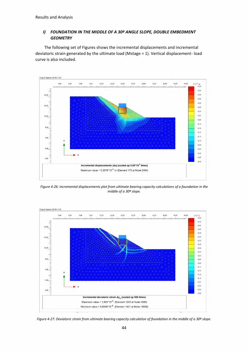
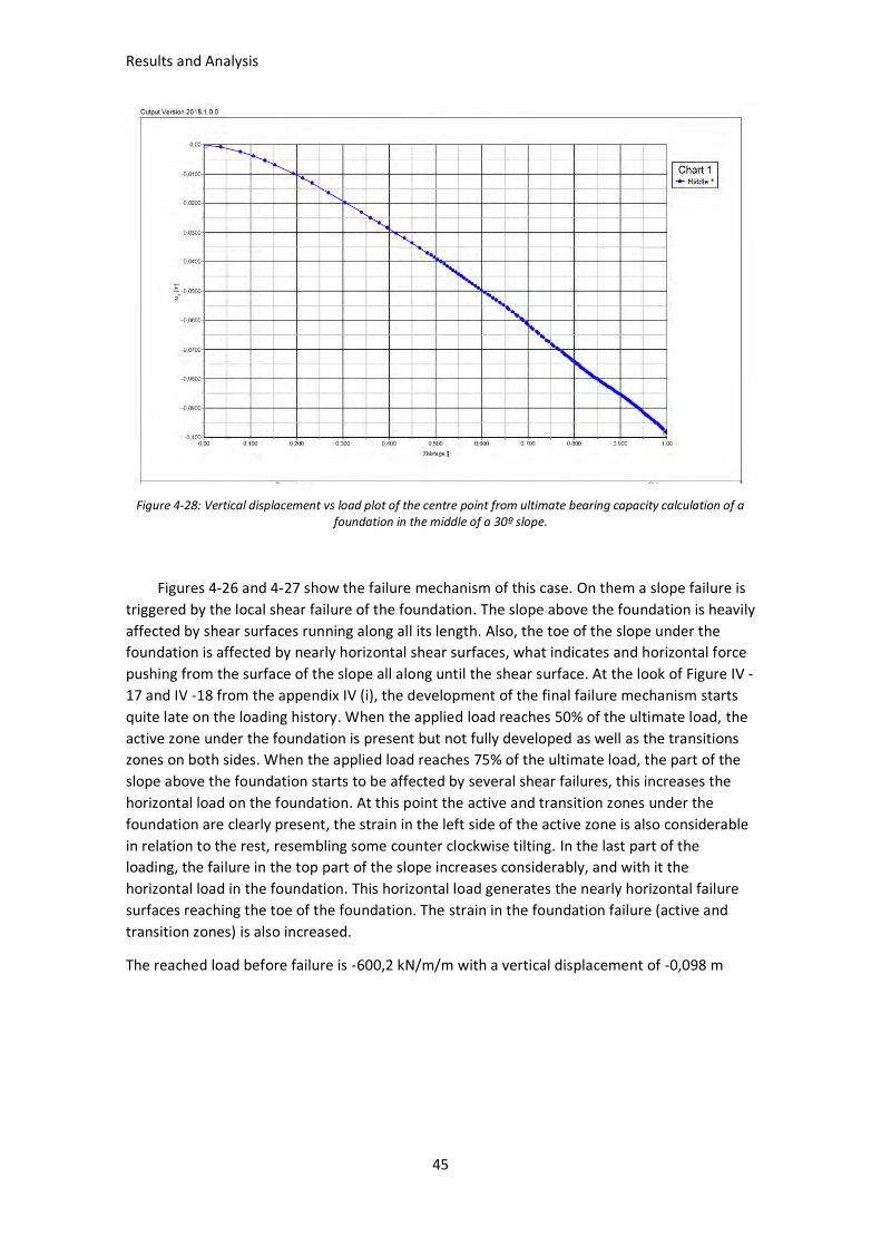
I) FOUNDATION IN THE MIDDLE OF A 30º ANGLE SLOPE, DOUBLE EMBEDMENT
GEOMETRY
The following set of Figures shows the incremental displacements and incremental
deviatoric strain generated by the ultimate load (Mstage = 1). Vertical displacement- load
curve is also included.
Figure 4-26: Incremental displacements plot from ultimate bearing capacity calculations of a foundation in the middle of a 30º slope.
Figure 4-27: Deviatoric strain from ultimate bearing capacity calculation of foundation in the middle of a 30º slope.
Results and Analysis
45
Figure 4-28: Vertical displacement vs load plot of the centre point from ultimate bearing capacity calculation of a foundation in the middle of a 30º slope.
Figures 4-26 and 4-27 show the failure mechanism of this case. On them a slope failure is
triggered by the local shear failure of the foundation. The slope above the foundation is heavily
affected by shear surfaces running along all its length. Also, the toe of the slope under the
foundation is affected by nearly horizontal shear surfaces, what indicates and horizontal force
pushing from the surface of the slope all along until the shear surface. At the look of Figure IV -
17 and IV -18 from the appendix IV (i), the development of the final failure mechanism starts
quite late on the loading history. When the applied load reaches 50% of the ultimate load, the
active zone under the foundation is present but not fully developed as well as the transitions
zones on both sides. When the applied load reaches 75% of the ultimate load, the part of the
slope above the foundation starts to be affected by several shear failures, this increases the
horizontal load on the foundation. At this point the active and transition zones under the
foundation are clearly present, the strain in the left side of the active zone is also considerable
in relation to the rest, resembling some counter clockwise tilting. In the last part of the
loading, the failure in the top part of the slope increases considerably, and with it the
horizontal load in the foundation. This horizontal load generates the nearly horizontal failure
surfaces reaching the toe of the foundation. The strain in the foundation failure (active and
transition zones) is also increased.
The reached load before failure is -600,2 kN/m/m with a vertical displacement of -0,098 m

Results and Analysis
46
J) FOUNDATION ON FLAT TERRAIN, DOUBLE EMBEDMENT GEOMETRY
The following set of Figures shows the incremental displacements and incremental
deviatoric strain generated by the ultimate load (Mstage = 1). Vertical displacement- load
curve is also included.
Figure 4-29: Incremental displacements plot from ultimate bearing capacity calculations of a foundation on flat terrain
Figure 4-30: Deviatoric strain from ultimate bearing capacity calculation of foundation on flat terrain

Results and Analysis
47
Figure 4-31: Vertical displacement vs load plot of the centre point from ultimate bearing capacity calculation of a foundation on flat terrain.
Figure 4-29 and 4-30 show the failure mechanism for this case. It is a local shear failure
from a foundation. The mechanism is symmetrical due to the isotropy of the model. It has an
active zone under the foundation and one passive zone on each side. Since is local shear failure
the shear surfaces don’t reach the surface of the soil. When looking at Figures IV -19 and IV -20
from appendix IV (j), the development of the failure mechanism can be explained. Initially the
active zone becomes present, when the load reaches 50% of the ultimate load this zone is still
developing (Figure IV -19). Then the passive zones start to appear, and the active zone
becomes smaller adopting the characteristic triangular shape. This can be seen when the load
reaches 75% of the ultimate load (Figure IV -20). Having this failure mechanism, symmetrical
and so close to the described by the theory reassures that the model is made correctly.
For the present case, the reached load before failure is – 1379 kN/m/m with a vertical
displacement of – 0,173 m
Results and Analysis
48
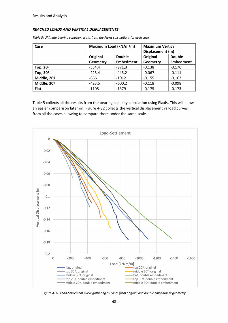
REACHED LOADS AND VERTICAL DISPLACEMENTS
Table 5: Ultimate bearing capacity results from the Plaxis calculations for each case
Case Maximum Load (kN/m/m) Maximum Vertical Displacement (m)
Original Geometry
Double Embedment
Original Geometry
Double Embedment
Top, 20º -554,4 -871,3 -0,138 -0,176
Top, 30º -223,4 -445,2 -0,067 -0,111
Middle, 20º -666 -1012 -0,155 -0,162
Middle, 30º -423,5 -600,2 -0,118 -0,098
Flat -1105 -1379 -0,175 -0,173
Table 5 collects all the results from the bearing capacity calculation using Plaxis. This will allow
an easier comparison later on. Figure 4-32 collects the vertical displacement vs load curves
from all the cases allowing to compare them under the same scale.
Figure 4-32: Load-Settlement curve gathering all cases from original and double embedment geometry
-0,2
-0,18
-0,16
-0,14
-0,12
-0,1
-0,08
-0,06
-0,04
-0,02
0
-1600-1400-1200-1000-800-600-400-2000
Ver
tica
l Dis
pla
cem
ent
[m]
Load [kN/m/m]
Load-Settlement
flat, original top 20º, originaltop 30º, original middle 20º, originalmiddle 30º, original flat, double embedmenttop 20º, double embedment top 30º, double embedmentmiddle 20º, double embedment middle 30º, double embedment
Results and Analysis
49
4.2 CYCLIC LOADING: CONSTANT VERTICAL FORCE RATIO
4.2.1 Input
The used soil parameters can be found in Table 3, being the same ones used for the
bearing capacity calculations. The applied forces for each case are calculated according to the
method described in Chapter 3.3.3 for keeping a constant ratio between bearing capacity and
applied load of 3,7. The used loads can be found in Table 6.
Table 6: Calculated forces for each case according to the method described in Chapter 3.3.3
Case Dead Load [kN/m] Maximum Load [kN/m]
Top of slope (20º) -210,7 -421,1
Top of slope (30º) -84,53 -169,1
Middle of slope (20º) -252 -504
Middle of slope (30º) -160 -320,5
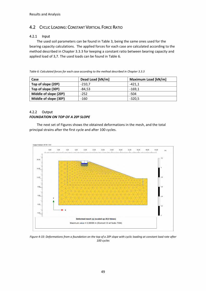
4.2.2 Output
FOUNDATION ON TOP OF A 20º SLOPE
The next set of Figures shows the obtained deformations in the mesh, and the total
principal strains after the first cycle and after 100 cycles.
Figure 4-33: Deformations from a foundation on the top of a 20º slope with cyclic loading at constant load rate after 100 cycles
Results and Analysis
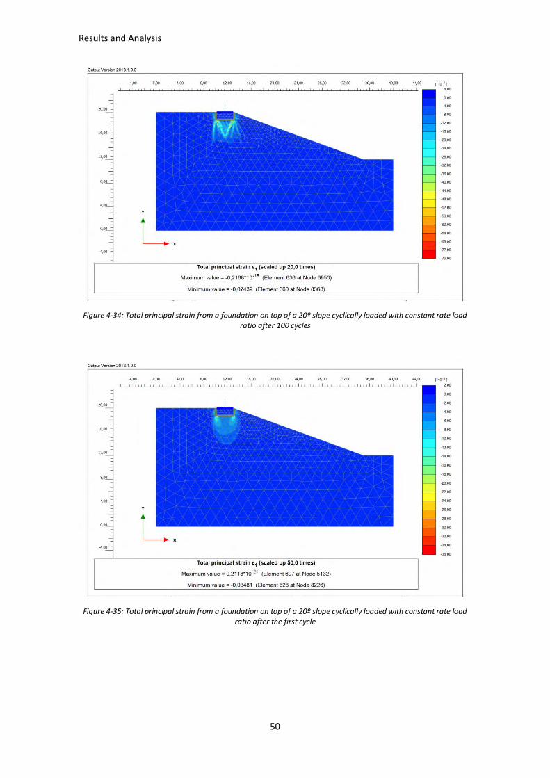
50
Figure 4-34: Total principal strain from a foundation on top of a 20º slope cyclically loaded with constant rate load ratio after 100 cycles
Figure 4-35: Total principal strain from a foundation on top of a 20º slope cyclically loaded with constant rate load ratio after the first cycle

Results and Analysis
51
The three following Figures gather the information related with vertical displacements as
well as amplitude of deformations within each cycle.
Figure 4-36: Vertical displacement of a foundation on top of 20º slope loaded with constant load ratio after 100 cycles. Vertical displacements taken in three points: middle (blue), right edge (red), left edge (purple).
Figure 4-37: Vertical displacement from a foundation on top of a 20º slope cyclically loaded with constant load ratio. Displacement of the middle point at no train load (blue) and with the maximum train load (orange)
-0,07
-0,06
-0,05
-0,04
-0,03
-0,02
-0,01
0
0 20 40 60 80 100 120
Ver
tica
l dis
pla
cem
ent
[m]
No. Cycles
Vertical Displacement
Displacement Dead Load Displacement Max Load

Results and Analysis
52
Figure 4-38: Deformations from a foundation in the top of a 20º slope loaded with constant load ratio. Total, plastic and elastic deformation within each cycle.
The shear surface develops starting from the edges of the foundation (Figure 4-35). At the
end of the cycles the active zone is fully present (Figure 4-34), the shear surface at the end
looks like the start of a foundation failure. The vertical displacement shows an inflexion point,
before the vertical displacement in each cycle is smaller than after. Passed the inflexion the
deformation per cycle is also fairly constant (Figure 4-37 and 4-38). Clockwise tilting is also
seen after the inflexion point (Figure 4-33 and 4-36). The plastic deformation in each cycle
seems to slightly increase until the inflexion point and remain with constant amplitude for the
rest of the cycles (Figure 4-38).
• Initial displacement with dead load is applied for first time: -0,012 m
• Displacement when first maximum train load is reached: -0,027 m
• Displacement at maximum train load in the last cycle: -0,061 m
• Displacement after last cycle: -0,059 m
• Inflexion point around cycle 32
• Tilt of the vertical displacement curve after inflexion: 0,02437
-0,016
-0,014
-0,012
-0,01
-0,008
-0,006
-0,004
-0,002
0
0,002
0 20 40 60 80 100 120D
efo
rmat
ion
[m
]
No. Cycle
Deformations/Cycle
Total Deformation
Plastic Deformation
Elastic Deformation
Results and Analysis
53
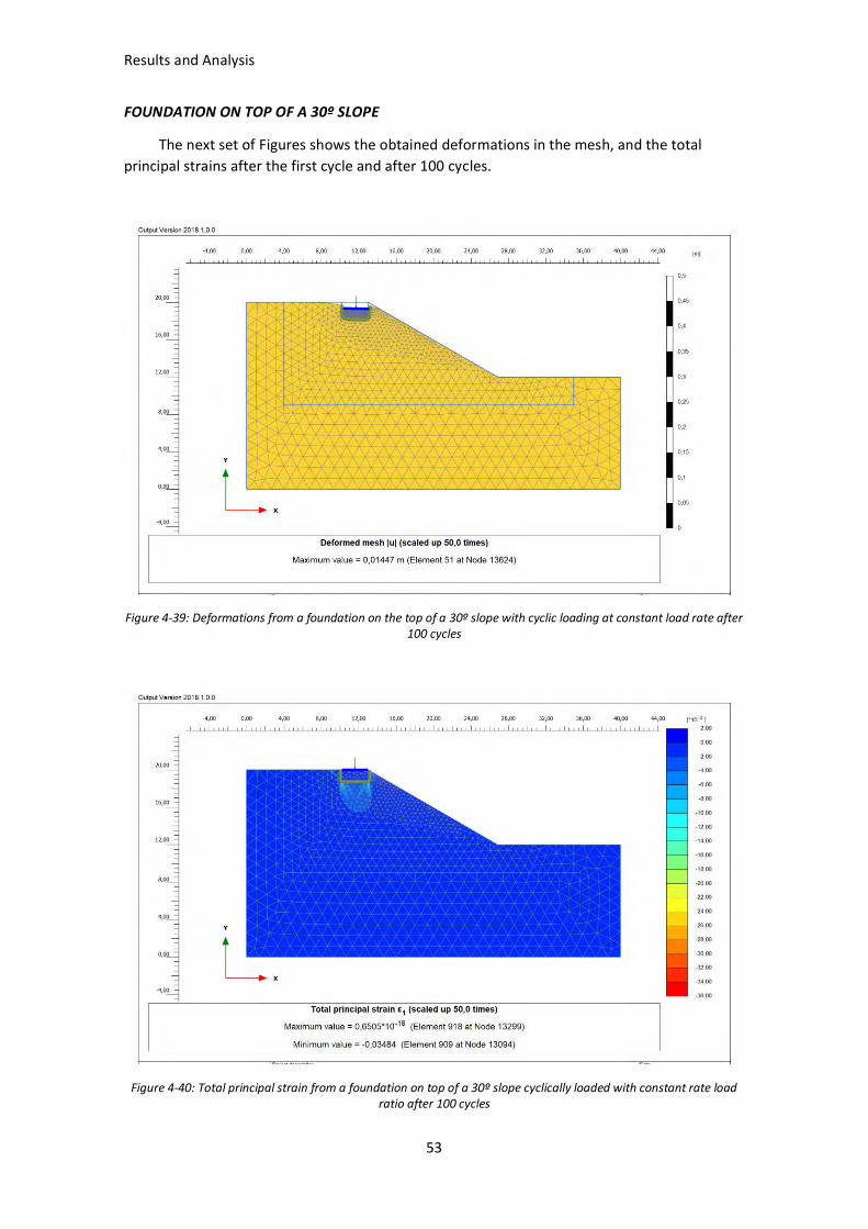
FOUNDATION ON TOP OF A 30º SLOPE
The next set of Figures shows the obtained deformations in the mesh, and the total
principal strains after the first cycle and after 100 cycles.
Figure 4-39: Deformations from a foundation on the top of a 30º slope with cyclic loading at constant load rate after 100 cycles
Figure 4-40: Total principal strain from a foundation on top of a 30º slope cyclically loaded with constant rate load ratio after 100 cycles

Results and Analysis
54
Figure 4-41: Total principal strain from a foundation on top of a 30º slope cyclically loaded with constant rate load ratio after the first cycle
The three following Figures gather the information related with vertical displacements as well
as amplitude of deformations within each cycle.
Figure 4-42: Vertical displacement of a foundation on top of 30º slope loaded with constant load ratio after 100 cycles. Vertical displacements taken in three points: middle (blue), left edge (red), right edge (purple).

Results and Analysis
55
Figure 4-43: Vertical displacement from a foundation on top of a 30º slope cyclically loaded with constant load ratio. Displacement of the middle point at no train load (blue) and with the maximum train load (orange)
Figure 4-44: Deformations from a foundation in the top of a 30º slope loaded with constant load ratio. Total, plastic and elastic deformation within each cycle
-0,016
-0,014
-0,012
-0,01
-0,008
-0,006
-0,004
-0,002
0
0 20 40 60 80 100 120
Dis
pla
cem
ent
[m]
No. Cycles
Vertical Displacement
Displacement Dead Load Displacement Max Load
-0,007
-0,006
-0,005
-0,004
-0,003
-0,002
-0,001
0
0,001
0 20 40 60 80 100 120
Dis
pla
cem
ent
[m]
No. Cycles
Deformation/Cycle
Total Deformation
Plastic Deformation
Elastic Deformation
Results and Analysis
56
The shear surface also develops from the edge of the foundation until the active zone is
developed (Figure 4-40 and 4-41). In this case the shear surfaces after 100 cycles seems to be
tilted towards the slope. The inflexion point is also present but not so obvious as in other cases
(Figure 4-43). A clockwise tilting is happening from the start of the loading, this can be seen in
Figure 4-42. The plastic deformation within the cycles Is small for this case also increasing after
the inflexion (Figure 4-44), the elastic deformation is almost constant for every cycle with a
very slight increase. The late development of the inflexion point can be an explanation of the
small plastic deformations obtained in this model.
• Initial displacement with dead load is applied for first time: -0,004 m
• Displacement when first maximum train load is reached: -0,011 m
• Displacement at maximum train load in the last cycle: -0,015 m
• Displacement after last cycle: -0,014 m
• Inflexion point around cycle 84
• Tilt of the vertical displacement curve after inflexion: 0,0372
FOUNDATION IN THE MIDDLE OF A 20º SLOPE
The next set of Figures shows the obtained deformations in the mesh, and the total
principal strains after the first cycle and after 100 cycles.
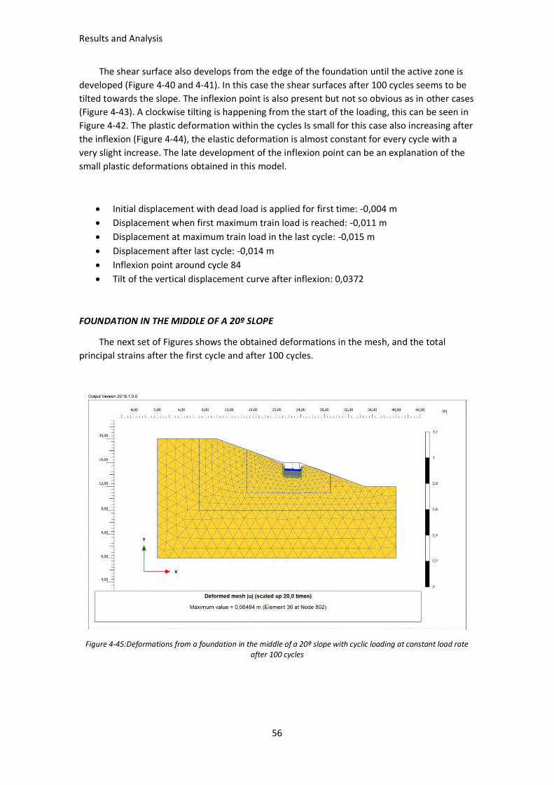
Figure 4-45:Deformations from a foundation in the middle of a 20º slope with cyclic loading at constant load rate after 100 cycles

Results and Analysis
57
Figure 4-46: Total principal strain from a foundation in the middle of a 20º slope cyclically loaded with constant rate load ratio after 100 cycles
Figure 4-47: Total principal strain from a foundation in the middle of a 20º slope cyclically loaded with constant rate load ratio after the first cycle
The three following Figures gather the information related with vertical displacements as well
as amplitude of deformations within each cycle.

Results and Analysis
58
Figure 4-48: Vertical displacement of a foundation in the middle of 20º slope loaded with constant load ratio after 100 cycles. Vertical displacements taken in three points: middle (blue), left edge (red), right edge (purple).
Figure 4-49:Vertical displacement from a foundation in the middle of a 20º slope cyclically loaded with constant load ratio. Displacement of the middle point at no train load (blue) and with the maximum train load (orange)
-0,07
-0,06
-0,05
-0,04
-0,03
-0,02
-0,01
0
0 20 40 60 80 100 120
Dis
pla
cem
ent
[m]
No. Cycles
Vertical Displacement
Displacement Dead Load Displacement Max Load

Results and Analysis
59
Figure 4-50: Deformations from a foundation in the middle of a 20º slope loaded with constant load ratio. Total, plastic and elastic deformation within each cycle
As seen in the previous cases the shear surface increases from the edges of the
foundation (Figure 4-46 and 4-47). At the end of the cycles the active zone is fully developed.
For this case the shear surfaces are tilted towards the slope (Figure 4-46). Also, the lower part
of the slope above the foundation is slightly affected by this shear surfaces. A clear inflexion
point is present. A bit before it the plastic deformations within each cycle starts increasing
(Figure 4-50 and 4-49) until they remain constant when the inflexion is passed. The clockwise
tilting of the foundation is also increasing until this inflexion, after it the foundation settles
evenly (Figure 4-48). The elastic deformation remains nearly constant with a slight increase
(Figure 4-50).
• Initial displacement with dead load is applied for first time: -0,011 m
• Displacement when first maximum train load is reached: -0,026 m
• Displacement at maximum train load in the last cycle: -0,062 m
• Displacement after last cycle: -0,060 m
• Inflexion point around cycle 40
• Tilt of the vertical displacement curve after inflexion: 0,02895
-0,016
-0,014
-0,012
-0,01
-0,008
-0,006
-0,004
-0,002
0
0,002
0 20 40 60 80 100 120D
efo
rmat
ion
[m
]
No. Cycles
Deformations/Cycle
Total Deformation Plastic Deformation Elastic deformation

Results and Analysis
60
FOUNDATION IN THE MIDDLE OF A 30º SLOPE
The next set of Figures shows the obtained deformations in the mesh, and the total
principal strains after the first cycle and after 100 cycles.
Figure 4-51: Deformations from a foundation in the middle of a 30º slope with cyclic loading at constant load rate after 100 cycles
Figure 4-52: Total principal strain from a foundation in the middle of a 30º slope cyclically loaded with constant rate load ratio after 100 cycles
Results and Analysis
61
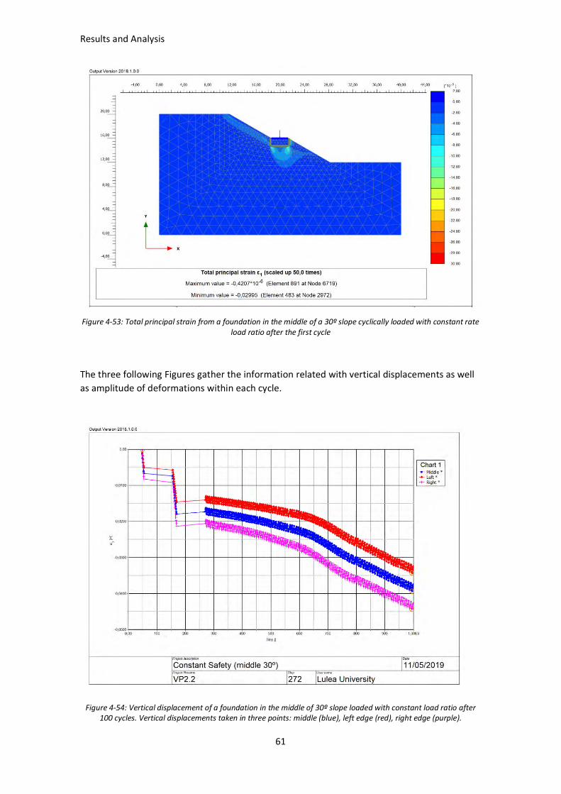
Figure 4-53: Total principal strain from a foundation in the middle of a 30º slope cyclically loaded with constant rate load ratio after the first cycle
The three following Figures gather the information related with vertical displacements as well
as amplitude of deformations within each cycle.
Figure 4-54: Vertical displacement of a foundation in the middle of 30º slope loaded with constant load ratio after 100 cycles. Vertical displacements taken in three points: middle (blue), left edge (red), right edge (purple).
Results and Analysis
62
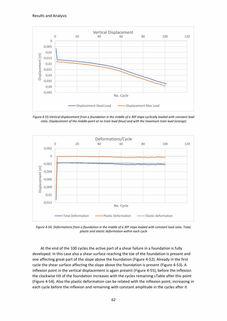
Figure 4-55:Vertical displacement from a foundation in the middle of a 30º slope cyclically loaded with constant load ratio. Displacement of the middle point at no train load (blue) and with the maximum train load (orange)
Figure 4-56: Deformations from a foundation in the middle of a 30º slope loaded with constant load ratio. Total, plastic and elastic deformation within each cycle
At the end of the 100 cycles the active part of a shear failure in a foundation is fully
developed. In this case also a shear surface reaching the toe of the foundation is present and
one affecting great part of the slope above the foundation (Figure 4-52). Already in the first
cycle the shear surface affecting the slope above the foundation is present (Figure 4-53). A
inflexion point in the vertical displacement is again present (Figure 4-55), before the inflexion
the clockwise tilt of the foundation increases with the cycles remaining sTable after this point
(Figure 4-54). Also the plastic deformation can be related with the inflexion point, increasing in
each cycle before the inflexion and remaining with constant amplitude in the cycles after it
-0,045
-0,04
-0,035
-0,03
-0,025
-0,02
-0,015
-0,01
-0,005
0
0 20 40 60 80 100 120D
isp
lace
men
t [m
]
No. Cycle
Vertical Displacement
Displacement Dead Load Displacement Max Load
-0,012
-0,01
-0,008
-0,006
-0,004
-0,002
0
0,002
0 20 40 60 80 100 120
Dis
pla
cem
ent
[m]
No. Cycle
Deformations/Cycle
Total Deformation Plastic Deformation Elastic deformation

Results and Analysis
63
(Figure 4-56). The elastic component of the deformation seems to be fairly constant with a
slight increase with the cycles.
• Initial displacement with dead load is applied for first time: -0,006 m
• Displacement when first maximum train load is reached: -0,018 m
• Displacement at maximum train load in the last cycle: -0,039 m
• Displacement after last cycle: -0,037 m
• Inflexion point around cycle 55
• Tilt of the vertical displacement curve after inflexion: 0,01849
4.3 CYCLIC LOAD: VERTICAL REAL LOAD
4.3.1 Input
The used soil parameters can be found in Table 3. Also, Table 7 shows the calculated
forces applied to each case. Since the load is too big for using with the original geometry, the
side of the foundation will be maintained at 2,8 m but the embedment will be doubled, 2,24m.
Table 7: Applied load for real load cases. Dead load corresponds to the dead load of the bridge that acts permanently, and maximum load is the maximum total load reached when the train passes
Case Dead Load [kN/m] Maximum Load [kN/m]
(Same to all) -336 -671,1
4.3.2 Output
FOUNDATION ON TOP OF A 20º SLOPE
The next set of Figures shows the obtained deformations in the mesh, and the total
principal strains after the first cycle and after 100 cycles.
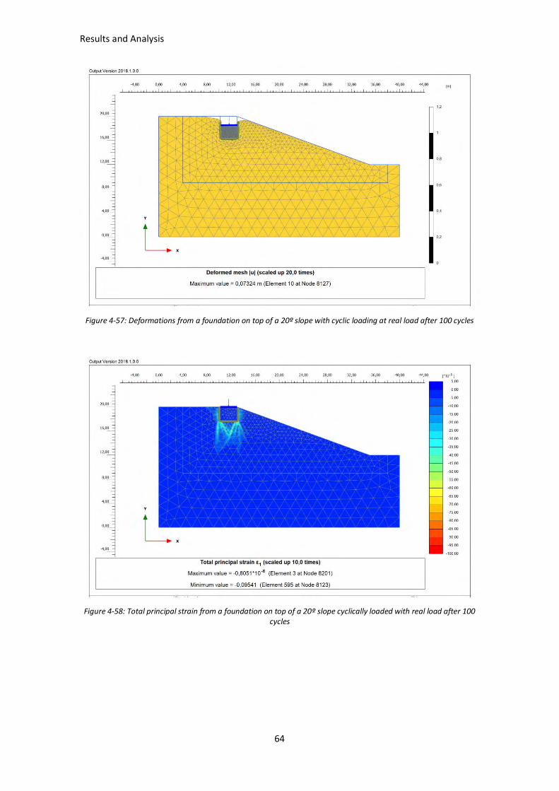
Results and Analysis
64
Figure 4-57: Deformations from a foundation on top of a 20º slope with cyclic loading at real load after 100 cycles
Figure 4-58: Total principal strain from a foundation on top of a 20º slope cyclically loaded with real load after 100 cycles

Results and Analysis
65
Figure 4-59: Total principal strain from a foundation on top of a 20º slope cyclically loaded with real load after the first cycle
The three following Figures gather the information related with vertical displacements as well
as amplitude of deformations within each cycle.
Figure 4-60: Vertical displacement of a foundation on top of 20º slope loaded with real load after 100 cycles. Vertical displacements taken in three points: middle (blue), left edge (red), right edge (purple).
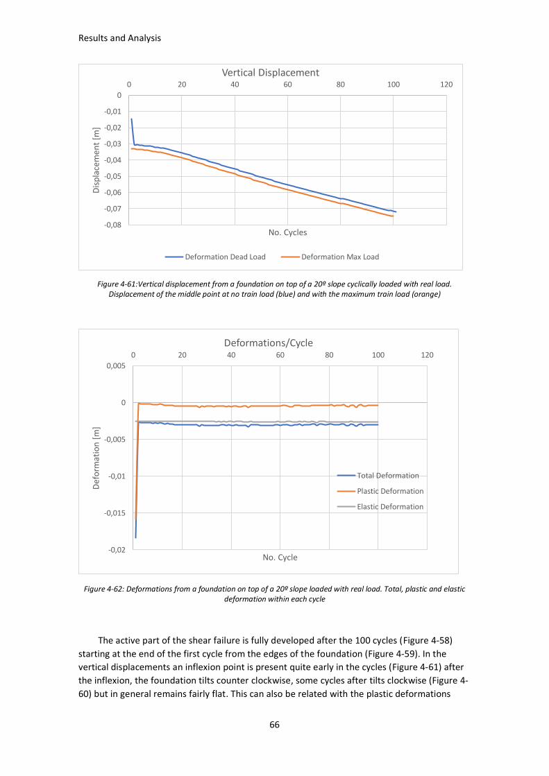
Results and Analysis
66
Figure 4-61:Vertical displacement from a foundation on top of a 20º slope cyclically loaded with real load. Displacement of the middle point at no train load (blue) and with the maximum train load (orange)
Figure 4-62: Deformations from a foundation on top of a 20º slope loaded with real load. Total, plastic and elastic deformation within each cycle
The active part of the shear failure is fully developed after the 100 cycles (Figure 4-58)
starting at the end of the first cycle from the edges of the foundation (Figure 4-59). In the
vertical displacements an inflexion point is present quite early in the cycles (Figure 4-61) after
the inflexion, the foundation tilts counter clockwise, some cycles after tilts clockwise (Figure 4-
60) but in general remains fairly flat. This can also be related with the plastic deformations
-0,08
-0,07
-0,06
-0,05
-0,04
-0,03
-0,02
-0,01
0
0 20 40 60 80 100 120
Dis
pla
cem
ent
[m]
No. Cycles
Vertical Displacement
Deformation Dead Load Deformation Max Load
-0,02
-0,015
-0,01
-0,005
0
0,005
0 20 40 60 80 100 120
Def
orm
atio
n [
m]
No. Cycle
Deformations/Cycle
Total Deformation
Plastic Deformation
Elastic Deformation

Results and Analysis
67
within each cycle shown in Figure 4-62. The plastic deformation amplitude increases after the
inflexion point, remaining stable for some cycles and slightly decreasing, the start of this
decrease can be matched with the cycles when the foundation starts tilting clockwise. The
elastic deformation is nearly constant.
• Initial displacement with dead load is applied for first time: -0,015 m
• Displacement when first maximum train load is reached: -0,033 m
• Displacement at maximum train load in the last cycle: -0,075 m
• Displacement after last cycle: -0,072 m
• Inflexion point around cycle 17
• Tilt of the vertical displacement curve after inflexion: 0,0258
FOUNDATION ON TOP OF A 30º SLOPE
The next set of Figures shows the obtained deformations in the mesh, and the total
principal strains after the first cycle and after 100 cycles.
Figure 4-63: Deformations from a foundation on top of a 30º slope with cyclic loading at real load after 100 cycles
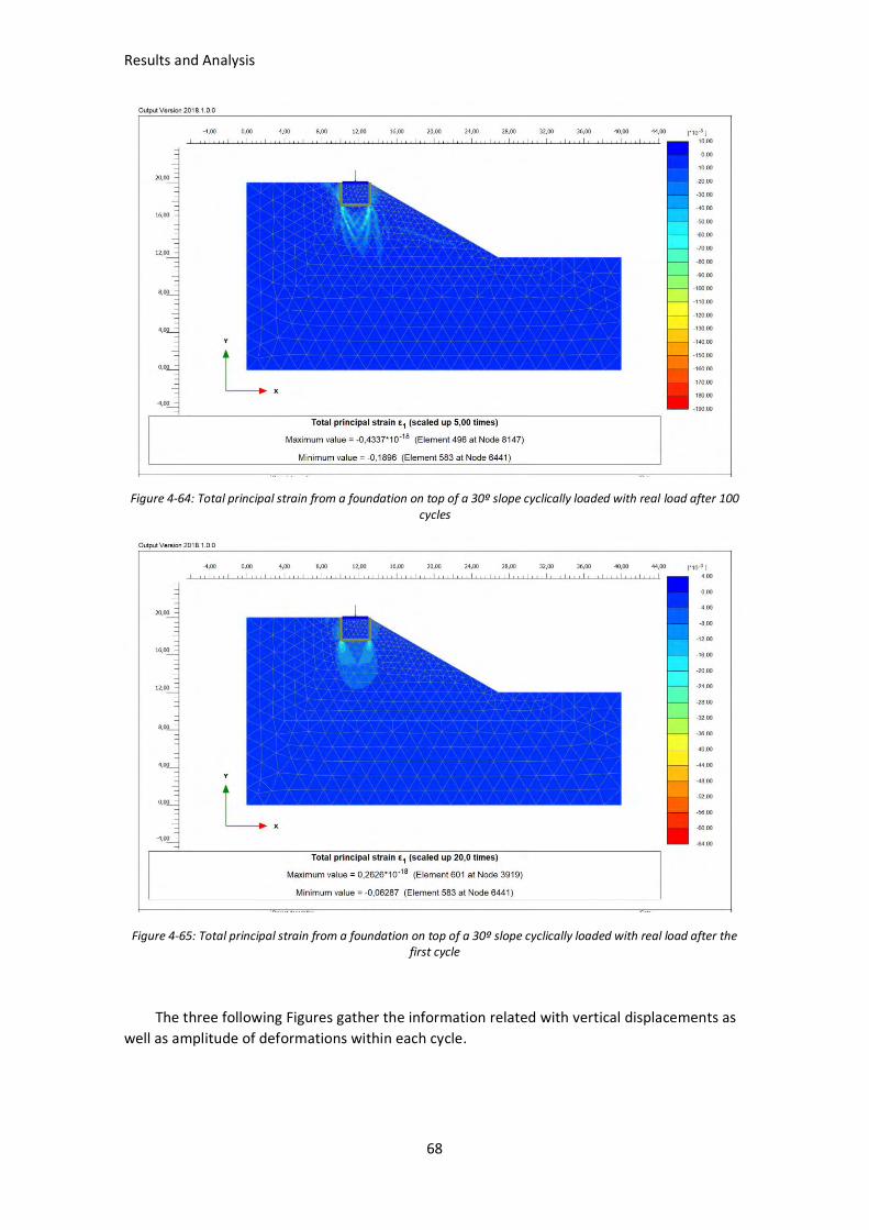
Results and Analysis
68
Figure 4-64: Total principal strain from a foundation on top of a 30º slope cyclically loaded with real load after 100 cycles
Figure 4-65: Total principal strain from a foundation on top of a 30º slope cyclically loaded with real load after the first cycle
The three following Figures gather the information related with vertical displacements as
well as amplitude of deformations within each cycle.
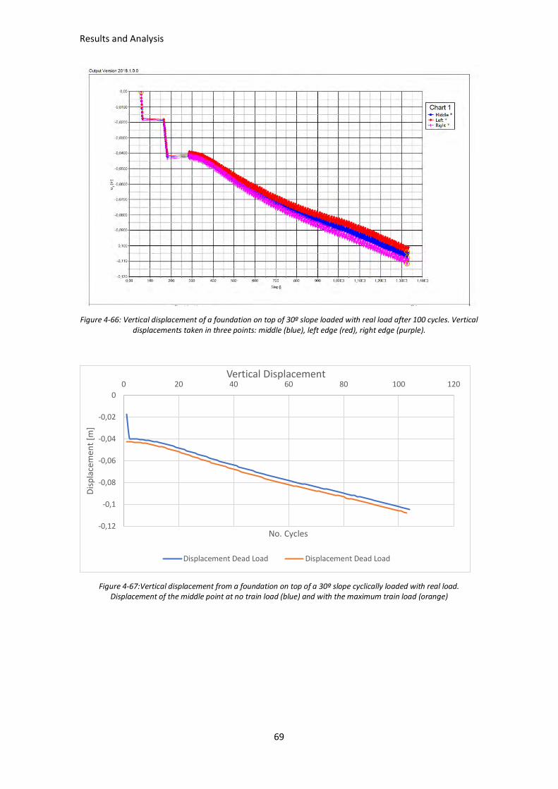
Results and Analysis
69
Figure 4-66: Vertical displacement of a foundation on top of 30º slope loaded with real load after 100 cycles. Vertical displacements taken in three points: middle (blue), left edge (red), right edge (purple).
Figure 4-67:Vertical displacement from a foundation on top of a 30º slope cyclically loaded with real load. Displacement of the middle point at no train load (blue) and with the maximum train load (orange)
-0,12
-0,1
-0,08
-0,06
-0,04
-0,02
0
0 20 40 60 80 100 120
Dis
pla
cem
ent
[m]
No. Cycles
Vertical Displacement
Displacement Dead Load Displacement Dead Load

Results and Analysis
70
Figure 4-68: Deformations from a foundation on top of a 30º slope loaded with real load. Total, plastic and elastic deformation within each cycle
For this case the active area of the shear failure is developed quite early in the cycles, in
Figure 4-65 is possible to see that after the first cycle it is almost formed. At the end of the 100
cycles it is fully developed, and it reaches great depth, seems to be tilted towards the slope.
Also, a shear surface towards the toe of the slope is starting to be present as well as one
affecting the soil on the left of the foundation. These two last surfaces can be the start of a toe
failure of the slope (Figure 4-64). The inflexion point in the vertical displacement curve (Figure
4-67) develops very early in the cycles. The foundation starts tilting form the first cycle,
increasing the rotation after the inflexion and remaining stable for the last cycles with even
settlement (Figure 4-66). This can be matched with the plastic deformation within each cycle
from Table 4-68, which increases the amplitude after the inflexion for later on decreasing it
and finally remain stable. The cycles with constant plastic amplitude are the same where the
foundation stops tilting.
• Initial displacement with dead load is applied for first time: -0,018 m
• Displacement when first maximum train load is reached: -0,043 m
• Displacement at maximum train load in the last cycle: -0,0108 m
• Displacement after last cycle: -0,0105 m
• Inflexion point around cycle 11
• Tilt of the vertical displacement curve after inflexion: 0,03735
-0,03
-0,025
-0,02
-0,015
-0,01
-0,005
0
0,005
0 20 40 60 80 100 120D
efo
rmat
ion
[m
]
No. Cycles
Deformations/Cycle
Total deformation
Plastic Deformation
Elastic Deformation
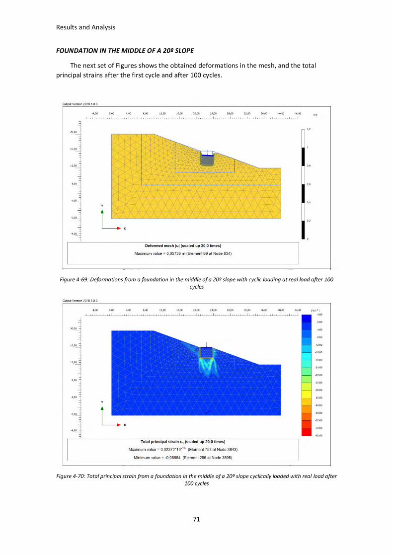
Results and Analysis
71
FOUNDATION IN THE MIDDLE OF A 20º SLOPE
The next set of Figures shows the obtained deformations in the mesh, and the total
principal strains after the first cycle and after 100 cycles.
Figure 4-69: Deformations from a foundation in the middle of a 20º slope with cyclic loading at real load after 100 cycles
Figure 4-70: Total principal strain from a foundation in the middle of a 20º slope cyclically loaded with real load after 100 cycles

Results and Analysis
72
Figure 4-71: Total principal strain from a foundation in the middle of a 20º slope cyclically loaded with real load after the first cycle
The three following Figures gather the information related with vertical displacements as
well as amplitude of deformations within each cycle.
Figure 4-72: Vertical displacement of a foundation in the middle of 20º slope loaded with real load after 100 cycles. Vertical displacements taken in three points: middle (blue), left edge (red), right edge (purple).

Results and Analysis
73
Figure 4-73:Vertical displacement from a foundation in the middle of a 20º slope cyclically loaded with real load. Displacement of the middle point at no train load (blue) and with the maximum train load (orange)
Figure 4-74: Deformations from a foundation in the middle of a 20º slope loaded with real load. Total, plastic and elastic deformation within each cycle
The present shear surfaces after 100 cycles are a fully developed active zone under the
foundation as well as some shear surfaces in the part of the slope above the foundation, as it
can be seen in Figure 4-70. As in the other cases the shear surfaces start from the edges of the
foundation (Figure 4-71). The vertical displacement curve from Figure 4-73 resembles an
inflexion point (Figure 4-73). From this inflexion point on the plastic deformation seems to
increase in amplitude in the following cycles for later on slightly decrease and remain stable
-0,06
-0,05
-0,04
-0,03
-0,02
-0,01
0
0 20 40 60 80 100 120D
isp
lace
men
t [m
]
No. Cycles
Vertical Displacement
Displacement Dead Load Displacement Max Load
-0,016
-0,014
-0,012
-0,01
-0,008
-0,006
-0,004
-0,002
0
0,002
0 20 40 60 80 100 120
Def
orm
atio
n [
m]
No. Cycle
Deformations/Cycle
Plastic Deformation Elastic deformation Total Deformation

Results and Analysis
74
(Figure 4-74). The tilting of the foundation is present since the first cycle but increase more
rapidly after the inflexion point it also seems to stop once the plastic deformation passes its
maximum and stabilizes (Figure 4-72).
• Initial displacement with dead load is applied for first time: -0,010 m
• Displacement when first maximum train load is reached: -0,025 m
• Displacement at maximum train load in the last cycle: -0,055 m
• Displacement after last cycle: -0,052 m
• Inflexion point around cycle 32
• Tilt of the vertical displacement curve after inflexion: 0,01994
FOUNDATION IN THE MIDDLE OF A 30º SLOPE
The next set of Figures shows the obtained deformations in the mesh, and the total
principal strains after the first cycle and after 100 cycles.
Figure 4-75: Deformations from a foundation in the middle of a 30º slope with cyclic loading at real load after 100 cycles

Results and Analysis
75
Figure 4-76: Total principal strain from a foundation in the middle of a 30º slope cyclically loaded with real load after 100 cycles
Figure 4-77:Total principal strain from a foundation in the middle of a 30º slope cyclically loaded with real load after the first cycle
The three following Figures gather the information related with vertical displacements as
well as amplitude of deformations within each cycle.

Results and Analysis
76
Figure 4-78: Vertical displacement of a foundation in the middle of 30º slope loaded with real load after 100 cycles. Vertical displacements taken in three points: middle (blue), right edge (red), left edge (purple).
Figure 4-79:Vertical displacement from a foundation in the middle of a 30º slope cyclically loaded with real load. Displacement of the middle point at no train load (blue) and with the maximum train load (orange)
-0,09
-0,08
-0,07
-0,06
-0,05
-0,04
-0,03
-0,02
-0,01
0
0 20 40 60 80 100 120
Dis
pla
cem
ent
[m]
No. Cycles
Vertical Displacement
Displacemenet Dead Load Displacement Max Load

Results and Analysis
77
Figure 4-80: Deformations from a foundation in the middle of a 30º slope loaded with real load. Total, plastic and elastic deformation within each cycle
From Figure 4-76, a fully active failure zone under the foundation is developed after 100
cycles. Also, there is a shear surface reaching the toe of the slope and one running along the
part of the slope above the foundation, strains in these two areas can be seen since the first
cycle (Figure 4-77). An inflexion point is present in the curve from Figure 4-79, developed early
during the cyclic loading. Clockwise tilting is present from the first cycle, seeming to be in the
middle part of the cycles but increasing again during the last part of the cyclic loading (Figure
4-78 and 4-75). Plastic deformation increases within each cycle after the inflexion point
remaining fairly constant after cycle 20. According to the elastic deformation it seems to be
constant (Figure 4-80).
• Initial displacement with dead load is applied for first time: -0,011 m
• Displacement when first maximum train load is reached: -0,028 m
• Displacement at maximum train load in the last cycle: -0,083 m
• Displacement after last cycle: -0,081 m
• Inflexion point around cycle 9
• Tilt of the vertical displacement curve after inflexion: 0,03390
-0,02
-0,015
-0,01
-0,005
0
0,005
0 20 40 60 80 100 120D
efo
rmat
ion
[m
]
No. Cycle
Deformations/Cycle
Total Deformation Plastic Deformation Elastic deformation
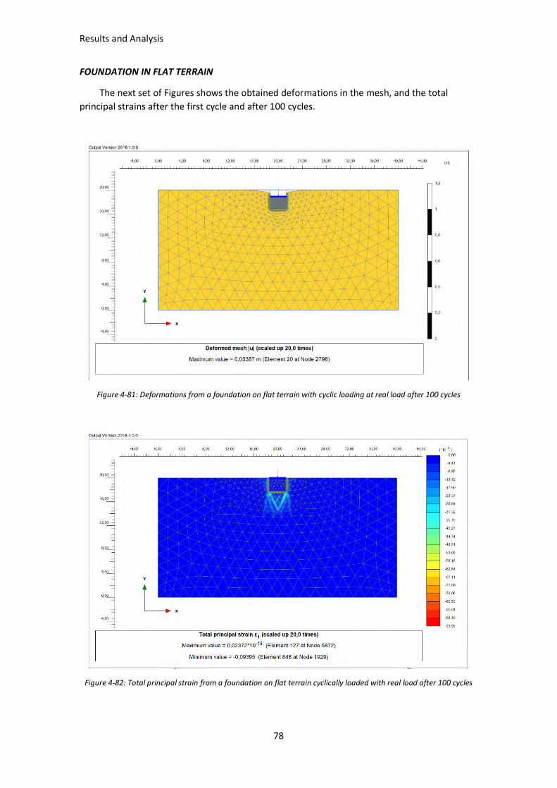
Results and Analysis
78
FOUNDATION IN FLAT TERRAIN
The next set of Figures shows the obtained deformations in the mesh, and the total
principal strains after the first cycle and after 100 cycles.
Figure 4-81: Deformations from a foundation on flat terrain with cyclic loading at real load after 100 cycles
Figure 4-82: Total principal strain from a foundation on flat terrain cyclically loaded with real load after 100 cycles

Results and Analysis
79
Figure 4-83:Total principal strain from a foundation on flat terrain cyclically loaded with real load after the first cycle
The three following Figures gather the information related with vertical displacements as
well as amplitude of deformations within each cycle.
Figure 4-84: Vertical displacement of a foundation on flat terrain loaded with real load after 100 cycles. Vertical displacements taken in three points: middle (blue), left edge (red), right edge (purple).

Results and Analysis
80
Figure 4-85:Vertical displacement from a foundation on flat terrain cyclically loaded with real load. Displacement of the middle point at no train load (blue) and with the maximum train load (orange)
Figure 4-86: Deformations from a foundation on flat terrain loaded with real load. Total, plastic and elastic deformation within each cycle
A fully developed active zone can be seen under the foundation in Figure 4-82, extending
from the edges of the foundation from the first cycle (Figure 4-83). The inflexion point in the
vertical displacement curve is also present but several cycles after it the vertical displacement
along the cycles seems to slow down (Figure 4-85). From Figure 4-81 and 4-84 no tilting is
present. Very small plastic deformation happens until the inflexion point is reached, after it the
amplitude of the plastic deformation within each cycle increases until cycle 60 approximately
when it reduces the amplitude and remain fairly constant for the rest of the cycles (Figure 4-
86). This reduction in the plastic deformation amplitude seems to match with the point when
-0,06
-0,05
-0,04
-0,03
-0,02
-0,01
0
0 20 40 60 80 100 120D
isp
lace
men
t [m
]
No. Cycles
Vertical Displacements
Displacement Dead Load Displacement Max Load
-0,016
-0,014
-0,012
-0,01
-0,008
-0,006
-0,004
-0,002
0
0,002
0 20 40 60 80 100 120
Def
orm
atio
n [
m]
No. Cycle
Deformation/Cycle
Total Deformation Plastic Deformation Elastic deformation

Results and Analysis
81
the vertical displacement starts increasing more slowly. The elastic deformation is nearly
constant with a slight increase.
• Initial displacement with dead load is applied for first time: -0,011 m
• Displacement when first maximum train load is reached: -0,026 m
• Displacement at maximum train load in the last cycle: -0,056 m
• Displacement after last cycle: -0,054 m
• Inflexion point around cycle 53
• Tilt of the vertical displacement curve after inflexion: 0,01740

Results and Analysis
82
4.4 CYCLIC LOADING: VERTICAL AND HORIZONTAL REAL LOAD
4.4.1 Input
For these calculations, soil parameters from Table 3 where used. As cyclic vertical load,
the values can be found in Table 7. The cyclic horizontal load and momentum will be applied
simulating a train passing from left to right in one case and from right to left in the other. The
values can be seen in Table 8. The geometry for a foundation on top of a 20º slope cyclically
loaded with vertical real load will be used for these cases.
Table 8: Cyclic horizontal load and momentum for simulating braking force.
Case Horizontal Load [kN/m] Momentum [kN·m/m]
Left to right 6,56 -26,25
Right to left -6,56 26,25
4.4.2 Output
BRAKING FORCE LEFT TO RIGHT
The next set of Figures shows the obtained deformations in the mesh, and the total
principal strains after the first cycle and after 100 cycles.
Figure 4-87: Deformations from a foundation on top of a 20º slope with cyclic loading (vertical and horizontal left to right) at real load after 100 cycles

Results and Analysis
83
Figure 4-88: Total principal strain from a foundation on top of a 20º slope cyclically loaded (vertical and horizontal left to right) with real load after 100 cycles
Figure 4-89:Total principal strain from a foundation on top of a 20º slope cyclically loaded (vertical and horizontal left to right) with real load after the first cycle
The three following Figures gather the information related with vertical displacements as
well as amplitude of deformations within each cycle.

Results and Analysis
84
Figure 4-90: Vertical displacement of a foundation on top of a 20º slope loaded with real load (vertical and horizontal left to right) after 100 cycles. Vertical displacements taken in three points: middle (blue), left edge (red),
right edge (purple).
Figure 4-91:Vertical displacement from a foundation on top of a 20º slope cyclically loaded (vertical and horizontal left to right) with real load. Displacement of the middle point at no train load (blue) and with the maximum train
load (orange)
-0,1
-0,09
-0,08
-0,07
-0,06
-0,05
-0,04
-0,03
-0,02
-0,01
0
0 20 40 60 80 100 120
Dis
pla
cem
ent
[m]
No. Cycles
Vertical Displacement
Displacement Dead Load Displacement Max Load

Results and Analysis
85
Figure 4-92: Deformations from a foundation on top of a 20º slope loaded with real load (vertical and horizontal left to right). Total, plastic and elastic deformation within each cycle
After 100 cycles a fully developed active zone under the foundation is present, bigger
strain can be seen in the right shear surface of the active zone (Figure 4-88). It started from the
edges of the foundation after the first cycle (Figure 4-89). Also, a shear surface is located on
the left of the foundation starting in the bottom left edge and reaching the surface of the flat
terrain. Increasing tilting of the foundation can be seen in Figure 4-90, starting from the first
loading cycle but increasing more rapidly along the cycles after the inflexion point in the
vertical displacement curve (Figure 4-91). Plastic deformation within each cycle seems to
increase around the inflexion point until its maximum around cycle 20. After this is remains
relatively constant with a slight decrease (Figure 4-92). Elastic deformation seems constant for
all cycles.
• Initial displacement with dead load is applied for first time: -0,015 m
• Displacement when first maximum train load is reached: -0,033 m
• Displacement at maximum train load in the last cycle: -0,091 m
• Displacement after last cycle: -0,089 m
• Inflexion point around cycle 12
• Tilt of the vertical displacement curve after inflexion: 0,03673
-0,02
-0,015
-0,01
-0,005
0
0,005
0 20 40 60 80 100 120D
efo
rmat
ion
[m
]
No. Cycle
Deformations/Cycle
Total Deformation Plastic Deformation Elastic deformation
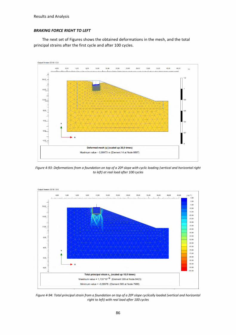
Results and Analysis
86
BRAKING FORCE RIGHT TO LEFT
The next set of Figures shows the obtained deformations in the mesh, and the total
principal strains after the first cycle and after 100 cycles.
Figure 4-93: Deformations from a foundation on top of a 20º slope with cyclic loading (vertical and horizontal right to left) at real load after 100 cycles
Figure 4-94: Total principal strain from a foundation on top of a 20º slope cyclically loaded (vertical and horizontal right to left) with real load after 100 cycles

Results and Analysis
87
Figure 4-95:Total principal strain from a foundation on top of a 20º slope cyclically loaded (vertical and horizontal right to left) with real load after the first cycle
The three following Figures gather the information related with vertical displacements as
well as amplitude of deformations within each cycle.
Figure 4-96: Vertical displacement of a foundation on top of a 20º slope loaded with real load (vertical and horizontal right to left) after 100 cycles. Vertical displacements taken in three points: middle (blue), right edge (red),
left edge (purple).
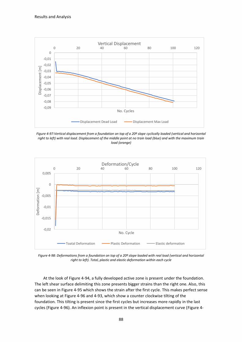
Results and Analysis
88
Figure 4-97:Vertical displacement from a foundation on top of a 20º slope cyclically loaded (vertical and horizontal right to left) with real load. Displacement of the middle point at no train load (blue) and with the maximum train
load (orange)
Figure 4-98: Deformations from a foundation on top of a 20º slope loaded with real load (vertical and horizontal right to left). Total, plastic and elastic deformation within each cycle
At the look of Figure 4-94, a fully developed active zone is present under the foundation.
The left shear surface delimiting this zone presents bigger strains than the right one. Also, this
can be seen in Figure 4-95 which shows the strain after the first cycle. This makes perfect sense
when looking at Figure 4-96 and 4-93, which show a counter clockwise tilting of the
foundation. This tilting is present since the first cycles but increases more rapidly in the last
cycles (Figure 4-96). An inflexion point is present in the vertical displacement curve (Figure 4-
-0,09
-0,08
-0,07
-0,06
-0,05
-0,04
-0,03
-0,02
-0,01
0
0 20 40 60 80 100 120
Dis
pla
cem
ent
[m]
No. Cycles
Vertical Displacement
Displacement Dead Load Displacement Max Load
-0,02
-0,015
-0,01
-0,005
0
0,005
0 20 40 60 80 100 120
Def
orm
atio
n [
m]
No. Cycle
Deformation/Cycle
Toatal Deformation Plastic Deformation Elastic deformation

Results and Analysis
89
97), during the cycles after the inflexion the amplitude of the plastic deformations within each
cycle starts increasing until it reaches the maximum around cycle 30. Elastic deformation
seems fairly constant with very slightly increase (Figure 4-98).
• Initial displacement with dead load is applied for first time: -0,015 m
• Displacement when first maximum train load is reached: -0,033 m
• Displacement at maximum train load in the last cycle: -0,082 m
• Displacement after last cycle: -0,079 m
• Inflexion point around cycle 15
• Tilt of the vertical displacement curve after inflexion: 0,02661
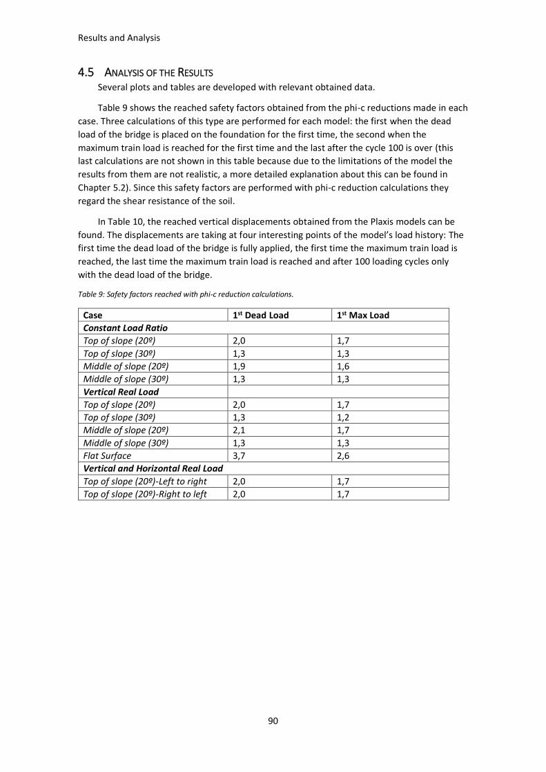
Results and Analysis
90
4.5 ANALYSIS OF THE RESULTS Several plots and tables are developed with relevant obtained data.
Table 9 shows the reached safety factors obtained from the phi-c reductions made in each
case. Three calculations of this type are performed for each model: the first when the dead
load of the bridge is placed on the foundation for the first time, the second when the
maximum train load is reached for the first time and the last after the cycle 100 is over (this
last calculations are not shown in this table because due to the limitations of the model the
results from them are not realistic, a more detailed explanation about this can be found in
Chapter 5.2). Since this safety factors are performed with phi-c reduction calculations they
regard the shear resistance of the soil.
In Table 10, the reached vertical displacements obtained from the Plaxis models can be
found. The displacements are taking at four interesting points of the model’s load history: The
first time the dead load of the bridge is fully applied, the first time the maximum train load is
reached, the last time the maximum train load is reached and after 100 loading cycles only
with the dead load of the bridge.
Table 9: Safety factors reached with phi-c reduction calculations.
Case 1st Dead Load 1st Max Load
Constant Load Ratio
Top of slope (20º) 2,0 1,7
Top of slope (30º) 1,3 1,3
Middle of slope (20º) 1,9 1,6
Middle of slope (30º) 1,3 1,3
Vertical Real Load
Top of slope (20º) 2,0 1,7
Top of slope (30º) 1,3 1,2
Middle of slope (20º) 2,1 1,7
Middle of slope (30º) 1,3 1,3
Flat Surface 3,7 2,6
Vertical and Horizontal Real Load
Top of slope (20º)-Left to right 2,0 1,7
Top of slope (20º)-Right to left 2,0 1,7

Results and Analysis
91
Table 10: Reached vertical displacements from each case
Case 1st Dead Load [m]
1st Max Load [m]
100 Cycles Max Load [m]
After 100 Cycles [m]
Inflexion Point Cycle Nº
Tilting after inflexion
Constant Load Ratio
Top of slope
(20º)
-0,012 -0,027 -0,061 -0,059 32 0,02437
Top of slope (30º)
-0,004 -0,011 -0,015 -0,014 84 0,03720
Middle of slope (20º)
-0,011 -0,026 -0,062 -0,060 40 0,02895
Middle of slope (30º)
-0,006 -0,018 -0,039 -0,037 55 0,01849
Vertical Real Load
Top of slope
(20º)
-0,015 -0,033 -0,075 -0,072 17 0,02580
Top of slope (30º)
-0,018 -0,043 -0,108 -0,105 11 0,03735
Middle of slope (20º)
-0,01 -0,025 -0,055 -0,052 32 0,01994
Middle of slope (30º)
-0,011 -0,028 -0,083 -0,081 9 0,0339
Flat Surface -0,011 -0,026 -0,056 -0,054 53 0,01740
Vertical and Horizontal Real Load
Top of slope (20º)-Left to right
-0,015 -0,033 -0,091 -0,089 12 0,03673
Top of slope
(20º)-Right to left
-0,015 -0,033 -0,082 -0,079 15 0,02661
In order to see and compare the vertical displacements and deformations per cycle from
each case with the others, they will be placed in a Figure with the same scale. All the cyclic
loading cases with vertical load are gathered in Figure 5-1. With the deformation per cycle
data, two sets of plots are done: one for the cases with constant load ratio and other for the
cases with vertical real load. Each set will have three Figures regarding total deformation per
cycle, plastic deformation per cycle and elastic deformation per cycle. The elastic deformation
plot is quite clear but the other two have too much noise due to the numerical calculations. A
polynomial interpolation has been done to clean the noise and obtain the general trend of the
results. Other set of Figures including all cases with cyclic real load (vertical, and vertical and
horizontal) related with a foundation on top of a 20º slope and the flat case is also made, the
same procedure as commented before is also followed for this set.

Results and Analysis
92
4.5.1 Cyclic Loading with Vertical Load
The following Figures shows the vertical displacement curves for the cyclic loading cases
only with horizontal loads and the deformations within each cycle, one set of Figures for the
cases with constant load ratio and other for the real force cases
Figure 4-99: Vertical displacement curves from all cases with cyclic vertical load
-0,12
-0,1
-0,08
-0,06
-0,04
-0,02
0
0 20 40 60 80 100 120
Ver
tica
l Dis
pla
cem
ent
[m]
No. Cycles
Vertical Displacement
top 20º, Real Load top 20º, Constant ratiotop 30º, Real Load top 30º, constant ratioMiddle 20º, Real Load middle 20º, constant ratiomiddle 30º, Real Load middle 30º, Constant Ratioflat, Real Load
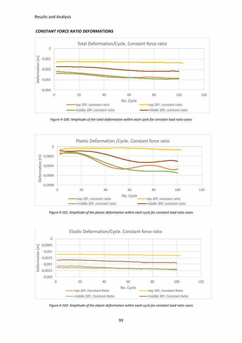
Results and Analysis
93
CONSTANT FORCE RATIO DEFORMATIONS
Figure 4-100: Amplitude of the total deformation within each cycle for constant load ratio cases
Figure 4-101: Amplitude of the plastic deformation within each cycle for constant load ratio cases
Figure 4-102: Amplitude of the elastic deformation within each cycle for constant load ratio cases
-0,004
-0,003
-0,002
-0,001
0
0 20 40 60 80 100 120
Def
orm
atio
n [
m]
No. Cycle
Total Deformation/Cycle. Constant force ratio
top 20º, constant ratio top 30º, constant ratio
middle 20º, constant ratio middle 30º, constant ratio
-0,0008
-0,0006
-0,0004
-0,0002
0
0 20 40 60 80 100 120
Def
orm
atio
n [
m]
No. Cycle
Plastic Deformation /Cycle. Constant force ratio
top 20º, constant ratio top 30º, constant ratio
middle 20º, constant ratio middle 30º, constant ratio
-0,003
-0,0025
-0,002
-0,0015
-0,001
-0,0005
0
0 20 40 60 80 100 120
Def
orm
atio
n [
m]
No. Cycle
Elastic Deformation/Cycle. Constant force ratio
top 20º, Constant Ratio top 30º, Constant Ratio
middle 20º, Constant Ratio middle 30º, Constant Ratio

Results and Analysis
94
VERTICAL REAL LOAD DEFORMATIONS
Figure 4-103: Amplitude of the total deformation within each cycle for vertical real load cases
Figure 4-104: Amplitude of the plastic deformation within each cycle for vertical real load cases
Figure 4-105: Amplitude of the elastic deformation within each cycle for vertical real load cases
-0,005
-0,004
-0,003
-0,002
-0,001
0 20 40 60 80 100 120
Def
orm
atio
n [
m]
No. Cycle
Total Deformation/Cycle. Real Load
top 20º, real loadtop 30º, real load middle 20º, real loadmiddle 30º, real load flat, real load
-0,001
-0,0005
0
0 20 40 60 80 100 120
Def
orm
atio
n [
m]
No. Cycle
Plastic Deformation /Cycle. Real Load
top 20º, real load
top 30º, real load middle 20º, real load
middle 20º, real load flat, real load
-0,0035
-0,003
-0,0025
-0,002
-0,0015
-0,001
0 20 40 60 80 100 120
Def
orm
atio
n [
m]
No. Cycle
Elastic Deformation/Cycle. Real Load
top 20º, Real Load top 30º, Real Load
middle 20º, Real Load middle 30º, Real Load
flat, Real Load
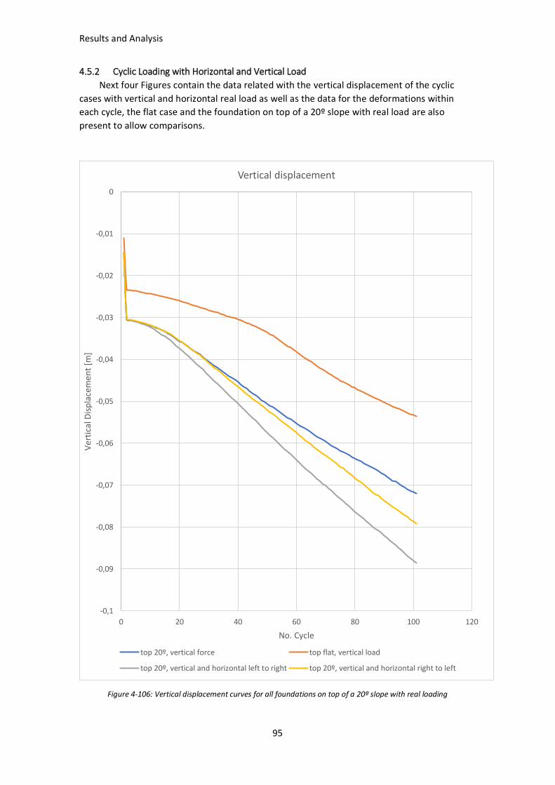
Results and Analysis
95
4.5.2 Cyclic Loading with Horizontal and Vertical Load
Next four Figures contain the data related with the vertical displacement of the cyclic
cases with vertical and horizontal real load as well as the data for the deformations within
each cycle, the flat case and the foundation on top of a 20º slope with real load are also
present to allow comparisons.
Figure 4-106: Vertical displacement curves for all foundations on top of a 20º slope with real loading
-0,1
-0,09
-0,08
-0,07
-0,06
-0,05
-0,04
-0,03
-0,02
-0,01
0
0 20 40 60 80 100 120
Ver
tica
l Dis
pla
cem
ent
[m]
No. Cycle
Vertical displacement
top 20º, vertical force top flat, vertical load
top 20º, vertical and horizontal left to right top 20º, vertical and horizontal right to left

Results and Analysis
96
FOUNDATION ON TOP OF A 20º SLOPE REAL LOAD DEFORMATIONS
Figure 4-107: Amplitude of the total deformation within each cycle for real load foundations on top of a 20º slope
Figure 4-108: Amplitude of the plastic deformation within each cycle for real load foundations on top of a 20º slope
Figure 4-109: Amplitude of the elastic deformation within each cycle for a real load foundation on top of a 20º slope
-0,004
-0,003
-0,002
-0,001
0 20 40 60 80 100 120
Def
orm
atio
n [
m]
No. Cycle
Total Deformation/Cycle
top 20º vertical flat, vertical
top 20º, vertical and horizontal left to right top 20º, vertical and horizontal right to left
-0,0008
-0,0006
-0,0004
-0,0002
0
0 20 40 60 80 100 120
Def
orm
atio
n [
m]
No. Cycle
Plastic Deformation/Cycle
top 20º, vertical flat, vertical
top 20º, vertical and horizontal left to right top 20º, vertical and horizontal right to left
-0,003
-0,0025
-0,002
-0,0015
-0,001
0 20 40 60 80 100 120
Def
orm
atio
n [
m]
No. Cycle
Elastic Deformation/Cycle
top 20º, vertical top flat, vertical
top 20º, vertical and horizontal left to right top 20º, vertical and horizontal right to left

Discussion
97
5 DISCUSSION
5.1 BEARING CAPACITY When comparing the results from the numerical simulations and the analytical methods
(Table 4 and Table 5), a good match can be seen. This increases the reliability of the results. As
the mentioned Tables show, the results from the models are very similar to the ones obtained
using Terzaghi’s method. Results from the French code are also in the range of the two
mentioned. These two methods only regard the case of foundations on top of a slope. Only
Meyerhof theory regards the case of foundations within the slope. For the case of a
foundation on top of the slope, Meyerhof results are in the range of 200 kN/m/m bigger than
the rest of the results. This is not a surprise since the theory is based on deep foundations.
When it comes to the foundations in the middle of the slope, Meyerhof results are also around
200 kN/m/m bigger than the ones obtained from Plaxis, this stable difference in the results
leads to think that the results from Plaxis related with the foundation in the middle of the
slope are also reasonable.
According to the results from Table 5, foundations placed in the middle of the slope have
bigger bearing capacity than the same ones on top of the slope. Also, bigger slope angles lead
to bigger reductions in bearing capacity. In the regarded cases, this effect is very remarkable
possibly by the proximity of the slope angle to the friction angle of the soil (since there is no
cohesion in the soil, the maximum allowed slope angle is equal to the friction angle). In
general, the cases with smaller or less shear surfaces tend to have less bearing capacity.
As mentioned in Chapter 2.2, the developed failure can be a foundation failure or slope
failure, or a combination of both. Ultimately, all the obtained failures resemble that the main
failure in the majority of the cases is related with the foundation. Since the aim of this set of
models is to find the bearing capacity, they can be considered as heavily loaded. As
commented in Pantelidis and Griffiths, 2014; heavily loaded foundations tend to show failures
related with foundations more than the slope.
When looking at the deviatoric strain plots from Chapter 4.1.3 al the failure mechanism
has at least one structure in common: a triangular active zone under the foundation with
transition zones on the sides is present resembling a local shear failure. This is also supported
by the shape of the curves in Figure 4-32, showing a great amount of plastic deformation
before failure (comparing with Figure 2-2). This basic structure is of course very affected by the
different characteristics of each case.
Figures 4-15 and 4-30 corresponding to the cases with foundations on flat terrain show a
clear local shear failure (compare with Figure 2-1). In these cases, the failure is symmetrical in
both sides of the foundation, changing the depth of the shear surfaces due to the change in
embedment. The differences from the rest of the models with this two are product only of
different slope angle and different position of the foundation in relation with the slope.
The cases with foundations on top of the slope with original embedment (Figure 4-2 and
4-6) present the same failure mechanism. The main parts of the local shear failure are present,
and they differ from the flat case on its lack of symmetry, being the failure developed on the
side of the slope. Both present also a shear surface running from the active zone towards the
surface of the slope but not reaching it. The case with 20º slope shows a longer shear surfaces

Discussion
98
and they affect the upper half part of the slope, when the slope is 30º the main shear surface
reaches nearly the toe of the slope.
Cases with original geometry and foundations in the middle of the slope have also the
same failure mechanism. The failure of this cases beside having the local shear failure
structure, seems that they also have an important component of slope failure. The active,
transition and passive zone is present in all of them. The part of the slope above of the
foundation presents failure signs in both cases (more important in the case with 30º slope).
This generates horizontal force in the foundation making the shear surface running from the
active zone towards the slope more active. In the case of 30º slope angle this failure reaches
the toe of the slope and is connected with the failure un the foundation above the foundation
(Figure 4-12). A deeper shear surface is present in both cases, it starts from the bottom left
corner of the foundation and resembles a base failure of the slope, it is more relevant in the
case with 20º angle slope (Figure 4-9).
For the cases with foundations on top of the slope and double embedment, the failure
mechanism seems very similar to the foundation in the middle of a slope with original
geometry but deeper. The local shear failure is again present with a bigger active zone than in
the cases with original geometry. Three well defined shear surfaces are also present but in
general does not reach the surface of the slope. The deepest starts from the bottom left
corner of the foundation and resembles the start of a base failure of the slope, more important
in the 20º case (Figure 4-18). Other runs from the active zone and seems to go in direction to
the toe of the slope but in both cases, it does not get close to the slope surface. The third one
starts from the middle of the active zone, nearly reaching the toe of the foundation in the case
of the 30º slope angle (Figure 4-21), the start of this surface seems to point towards the small
shear surface on the left of the foundation reaching the flat surface.
Finally, the cases with foundations in the middle of a slope and double of the original
embedment, are the ones with more complex failure mechanism. The active zone under the
foundation, and the transition zones are present in both cases what shows the local failure
component of the foundation. In the case of 20º slope angle (Figure 4-24) the transition and
passive zone in right are well developed and deep, no shear failure touches the slope surface.
In both cases the part of the slope above the foundation is heavily affected (important shear
surfaces along the full length of it in the case of 30º slope). This generates important horizontal
forces in the foundation, producing even a horizontal flat surface reaching the toe of the slope
in the 30º slope case (Figure 4-27). In both cases, shear surfaces with important strains are
present starting from the right bottom corner of the foundation and running in the opposite
direction than to the slope, this can be due to the horizontal force in the foundation that
makes it tilt clockwise. This surface is more relevant in the case with 20º slope angle.
The way failure mechanisms are developed is also quite similar for all the cases. First the
active zone is developed, in cases of 20º slope is normally already present when the load is
50% the ultimate load (Figure IV-11), cases with 30º slope tend to develop it after this load
(Figure IV-3). Also, before 50% of the ultimate load some strain is happening in the part of the
slope above the foundation for the cases with foundations in the middle of the slope (Figure
IV-7). In between 50% and 75% of the ultimate load, the part of the failure corresponding the
local shear failure of the foundation is generally developed (Figure IV-12). At this point nearly
all cases on slope, develop the shear failure starting from the active zone and pointing towards
the slope. In cases with foundation in the middle of the slope, the strain in the part above the

Discussion
99
foundation increases (This is more notable in cases with 30º slope). Finally, between 75% and
100% of the ultimate load the rest of the failure mechanism is developed.
The behaviour of the failure in foundations horizontally loaded according to the amount
of vertical load on them described by Taeseri 2017 (Figure 2-9), can be seen in some of the
models with bigger horizontal loads (foundation on the middle of a slope with double
embedment). When the foundations are not fully loaded, the principal shear failure tends to
develop in the same direction as the applied horizontal load (for these cases from left to right)
and generate a counter clockwise tilting. Figures resembling this are IV-16 and IV-18. When the
full load is applied, the mentioned shear surfaces seems to loose importance and the strain is
concentrated in surfaces with the opposite direction to the horizontal load applied, changing
the tilting direction (Figure 4-24 and 4-27).
5.2 CYCLIC VERTICAL LOADING Continuing with the topic of slope failure vs foundation failure, the constant load ratio
cases have a ratio of 3,7 between bearing capacity and applied load. This can be seen as a
traditional safety factor against vertical load for a foundation. When comparing the safety
factors obtained from the phi-c reduction calculations of this cases after applying the
maximum load (dead load and maximum train load) the results are around 1,7 for the cases
with 20º slopes and 1,3 for the cases with 30º slope. This safety factors are related with the
shear strength of the model, meaning that is more similar to the normal approach of analysing
slopes. It can be seen that the factors of safety about the half of the one against vertical load.
This proves two things: first the strong influence of the slope failure in the problem, and
second the necessity of checking both failure mechanism when assessing this kind of
problems.
On the other hand, this safety factors shows one limitation of the model. The safety
factors at the start and at the end of the cycles ares the same for every case. In reality, this is
not possible once deformation takes place. This is related with the activated dilatancy that the
model does not take into account for the safety calculation. To check it in the case of the
foundation on top of a 20º slope with double embedment geometry, the ultimate bearing
capacity load was placed in the foundation after the cycles. The result is that the foundation
can no longer hold this load, being reduced the bearing capacity by around a 10%.
Figure 4-99 and 4-106 show the vertical displacements along the cycles of the middle
point of the foundation in each case. It is possible to see that regardless of the case the general
shape of the displacement is very similar between all, showing an inflexion point that divides
the curve in two zones, before with a slower vertical displacement and after with faster
vertical displacement. Many of the obtained results can be related with this inflexion point.
The approximate cycle when the inflexion takes place for each case can be seen in Table 10.

Discussion
100
Beside when the inflexion appears the mechanism seems to be the same in all cases.
When comparing the plots of total principal strain from all cyclic cases (Chapter 4.2, 4.3 and
4.4) it can be seen for all cases that at the end of the 100 cycles a fully developed active zone
under the foundation is present. In the same way, after the first loading cycle a small start of
the shear surfaces that delimitate the active zone is present in the bottom edges of the
foundation. If this same plot is checked few cycles before the inflexion (Figure 5-1 a and c) the
two shear surfaces are already developed but they have not formed the triangular active zone.
Once this triangle is fully formed the inflexion takes place (Figure 5-1 b and d).
According to the sinking speed after the inflexion point, it seems to be highly related with
slope angle. Table 10 shows that the slowest sinking speed is the foundation in the flat terrain,
the foundations in slopes of 20º have slower sinking speed than the cases in slopes of 30º.
Beside the foundation in flat terrain (Figure 4-62), all the cases present tilting of the
foundation. Except a couple of exceptions where there is a great amount of tilting in the first
cycle (Figure 4-23 and 4-35), the tilt of the foundation starts some cycles before the inflexion
and increases the amplitude per cycle until some cycles after the inflexion. At this point it
becomes stable. Also, a bigger amount of tilting is present in the cases with 30º slope.
Regarding the generated shear surfaces in the models, all of them show a fully developed
active zone under the foundation at the end of 100 cycles (as an example Figure 4-15 and 4-57
can be seen). The active appear tilted towards the slope in the cases of the foundation in the
middle of the slope, with a bigger tilt when the slope is 30º. Also, these cases show shear
surfaces running along the slope above the foundation, being maybe an explanation about the
a)
b)
c)
d)
Figure 5-1: Total principal strains few cycles before the inflexion point (a, c) and few cycles after (b, d) for
foundation on top of a slope with real load (a, b) and in the middle of a slope with constant load ratio (c, d).

Discussion
101
tilt of the active zone due to the horizontal force that the soil between the shear surface and
the surface of the slope generate in the left side of the foundation (explaining also why these
cases show the biggest rotations in the foundation). Also some cases with 30º slope show
shear surfaces resembling toe slope failures (see Figure 4-33 and 4-45) reassuring the
important role of the slope angle in the bearing behaviour of this problems.
When comparing the shear surfaces of the cyclic models and the bearing capacity ones is
clear that they do not follow the same path. Shear surfaces that look like slope failures are
present in some of the cyclic loading, but they are more common in the models loaded until
failure. The foundation failure developed in the bearing capacity cases is a local shear failure
compared to the cyclic cases which resembles a punching failure.
For concluding a look to the deformations per cycle will be made. From Figure 4-100 to
Figure 4-105 the curves with total, plastic and elastic deformations in the cases with cyclic
vertical load are gathered. Generally, the amplitude of the elastic deformation in each cycle is
rather constant with a very small increase along the cycles. The plastic deformation increases
the amplitude in each cycle until the inflexion point. After, it decreases the amplitude and
remains fairly constant (some fluctuations can be seen in certain cases, but it can be more to
the interpolation from the original results than a real fluctuation). Again, it is seen that the
value of the amplitude is more related to the slope angle than to other parameters. Slopes
with more inclination give more plastic deformation amplitude in the cases of constant load
ratio and smaller one in the cases with real load. The shape of the curves in Figure 5-6 can also
be related with the position of the slope, the increase and decrease in amplitude around the
inflexion point is bigger in the cases with the foundation on top of the slope.
In general, the cases can be classified as stepwise failure according to Goldscheider and
Gudehus, 1976. Even if there are some small variations in the amplitude of the plastic
deformation, it never disappears completely and it does not decreases constantly with the
cycles. Also, as pointed by Wichtmann, 2005; the first cycle is where the biggest plastic
deformation takes place. Although, for surely know what kind of behaviour related with the
plastic deformation more cycles have to be done.
5.3 CYCLIC VERTICAL AND HORIZONTAL LOADING Many of the observations made for the cyclic vertical loading cases are also applicable to
these cases. Figure 5-8 shows the relation between the vertical displacement curves, the flat
case and the foundation on top of a 20º slope with real loading are also added for comparison.
The case in flat terrain is the one with less vertical deformation and less deformation speed. Is
interesting how the rest cases follow the same curve at the start, until the case with horizontal
force from left to right reaches its inflexion point (this case hast the fastest vertical
displacement between the ones in this Figure). The other two cases continue throw the same
path some more cycles until the one with horizontal force from right to left increases the
sinking speed. When comparing the reached vertical displacements in Table 10, all the cases
on slope have the same displacements during the first cycle.
The foundations tilt according to the applied momentum and horizontal force, showing an
always increasing clockwise rotation for the case with horizontal force left to right (Figure 4-
71) and a counter clockwise for the other case (Figure 4-77), in this last case the rotation only
seems to increase with the cycles along the last cycles.

Discussion
102
The developed shear surfaces are, as in every case, the ones related with the active zone
under the foundation. These cases also show some particular shear surfaces from the bottom
edge of the foundation to the surface of the soil, in the right of the foundation for the case
with horizontal force from right to left (Figure 4-75) and on the left for the other case (Figure
4-69). These surfaces are developed by the rotation of the foundation.
Elastic deformation has the same behaviour as the cases with vertical load and does not
seem very affected by the horizontal loads and momentums (Figure 4-109). The biggest plastic
deformation amplitude in the cycle is seen in the case with horizontal force from left to right.
Also, when this deformation decreases after the inflexion, it has the slowest decrease from all
the cases. Beside the flat terrain the three other curves have the same shape.

Conclusion and Future Work
103
6 CONCLUSION AND FUTURE WORK
The purpose of the present thesis has been to study the bearing capacity of railway bridge
foundations related to slopes under heavy loads. As a conclusion it can be said:
• The bearing capacity and failure mechanism depends strongly in the position of the
foundation, angle of the slope and embedment. The angle of the slope seems to be
the one affecting more the bearing capacity, reducing it considerable with bigger slope
angles. Bigger embedment gives bigger bearing capacities and foundations in the
middle of the slope generally have also bigger bearing capacities, but they have the
inconvenient of the horizontal load generated by the part of the slope above them.
• Local shear failure is the predominant failure mode when the models where statically
loaded until failure. Some cases, generally related with big slope angles or big
horizontal loads generated by the slope, present a combination between slope failure
and foundation failure.
• Traditional bearing capacity safety factors are not accurate for this type of problems.
The influence of the slope has also to be taken into account with shear strength
calculations.
• The present shear failures when the foundations are cyclically loaded resembles a
punching failure. As in the static case, models with bigger slopes and horizontal forces
also have a slope failure component in the mechanism.
• An inflexion point from where the vertical displacement increases the speed during
the cyclic loading is present in all cases. This point is related with the formation of an
active zone under the foundation and mainly is affected by the slope angle and the
embedment.
• Deformations within each cycle tend to increase until the inflexion point and then
remain more or less stable. Elastic deformation is constant along all cycles with a slight
increase in amplitude. Plastic deformation increases its amplitude until the inflexion
point, after it the amplitude reduces slightly and the remains constant.
Since this is the first approach to the problem, further investigation has to be done.
Physical experiments can be performed as well as data collection from real sites. Also, the
cases can be tested with more slope angles in order to see the transition from 20º slope to
30º. Sea page can be added to the system to check how the failures and bearing capacities
vary with water in the system, this is important in cyclic loading due to the pore pressure
development. In this thesis the foundations where loaded with 100 cycles, to further
investigate the failure mechanism, would be interesting to see situation at a bigger number of
cycles. For a complete understanding, several geometries can be tested.

References
104
7 REFERENCES
• Chen, W.F. & Duan, L. (2000). Bridge Engineering Handbook. Boca Raton: CRC Press.
• Das, B.M. (2011). Principles of Foundation Engineering (7 ed.). Cengage Learning.
• DTU 13.11 & 13.12. French code of shallow foundations.
• Fryba, L. (1996). Dynamics of Railway Bridges. Academy of Sciences of the Czech
Republic, Prague.
• Goldscheider, M. & Gudehus, G. (1976). Einige bodenmechanische Probleme bei
Küstenund Offshore-Bauwerken. In Vortr•age zur Baugrundtagung 1976.
• Knappett, J.A. & Craig, F. (2012). Craig’s Soil Mechanics (8 ed.). New York: Spon Press.
• Lang, H.J. & Huder, J. & Amann, P. (2003). Bodenmechanik und Grundbau: Das
Verhalten von Böden und Fels und die wichtigsten grundbaulichen Konzepte. Springer
International Publishing.
• Masing, G. (1926). Eigenspannungen und Verfestigung Beim Messing. In In Proc. 2nd
Int. Congr. Appl. Mech. Zurich
• Meyerhof, G.G. (1957) The Ultimate Bearing Capacity of Foundations on Slopes. 4th
International Conference on Soil Mechanics and Foundation Engineering, 3, 384-386
• Pantelidis, L. & Griffiths, D.V. (2014). (2015). Footing on the Crest of Slope: Slope
Stability or Bearing Capacity?. In Engineering Geology for Society and Territory-Volume
2 (pp. 1231-1234). Springer International Publishing.
• PLAXIS. (2018). Material Models Manual. Retrieved 15 January 2019 from
https://www.plaxis.com/support/manuals/plaxis-2d-manuals/
• PLAXIS. (2018). Reference Manual. Retrieved 15 January 2019 from
https://www.plaxis.com/support/manuals/plaxis-2d-manuals/
• Taeseri, D. (2017). The Non-Linear Behaviour of Foundations in Slopes During Seismic
Events. Doctoral Thesis. ETH Zurich.

References
105
• Terzaghi, K. (1943). Theoretical Soil Mechanics, New York: Wiley.
• Unsworth, J.F. (2017). Design and Construction of Modern Steel Railway Bridges (2
ed.). Boca Raton: Taylor & Francis, CRC Press.
• Wichtmann, T. (2005). Explicit Accumulation Model for Non-Cohesive Soils Under Cyclic
Loading. Ruhr-University, Bochum.

Appendix I: Soil Model Selection
106
APPENDIX I: SOIL MODEL SELECTION
Two soil models were regarded before starting to make the calculations: Mohr-Coulomb
soil model and Small Strain Hardening soil.
Information about the Small Strain Hardening Soil model can be found in Chapter 2.5.
Mohr-Coulomb soil model is a perfectly plastic linear elastic model. The linear elastic
behaviour in this model is based in Hooke’s law and the plasticity rule in the Mohr-Coulomb
failure criterion (Plaxis, 2018). This criterion has a fixed yield surface independent on load or
strain history.
Two cases where tested with both soil models in order to determine which is more suitable:
bearing capacity of a foundation on top of a 20º slope with original geometry and bearing
capacity of a foundation in the middle of a 20º slope with original geometry.
Figure I-1: Incremental displacements of a foundation on top of a 20º slope, Mohr-Coulomb soil model.

Appendix I: Soil Model Selection
107
Figure I-2: Incremental displacements for a foundation in the middle of a 20º slope. Mohr-Coulomb soil model.
When comparing Figure I-1 and I-2 with Figure 4-1 and 4-8 (which corresponds to the
same cases calculated with Small Strain Hardening Soil), is quite clear that the results are not
the same. Taking a look to the reached maximum bearing capacity loads, in the case of the
foundation on top of the slope calculated with Mohr-Coulomb gives -315,95 kN/m/m; way
smaller than the reached value calculated with Small Strain and also not very close to the
results from the analytical methods. In the case of a foundation in the middle of the slope, the
reached loads are quite similar in both cases, being the maximum allowed load -622,71
kN/m/m from the Mohr-Coulomb calculations. Related to the failure mechanisms obtained
from the Mohr-Coulomb models, it is important to say that are completely different to the
ones from Small Strain Hardening Soil. They are way smaller and doesn’t resemble to any
expected failure mechanism.
Since the Small Strain hardening soil gives closer results to the analytical solutions, the
failure mechanisms seem more realistic and it properly models the non-linear changes in
stiffness of the soil, it is the models that is going to be used for all the studied models.
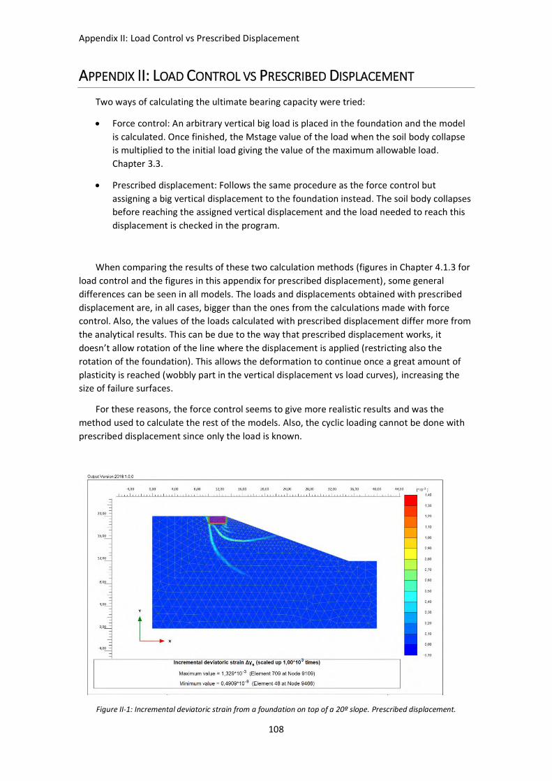
Appendix II: Load Control vs Prescribed Displacement
108
APPENDIX II: LOAD CONTROL VS PRESCRIBED DISPLACEMENT
Two ways of calculating the ultimate bearing capacity were tried:
• Force control: An arbitrary vertical big load is placed in the foundation and the model
is calculated. Once finished, the Mstage value of the load when the soil body collapse
is multiplied to the initial load giving the value of the maximum allowable load.
Chapter 3.3.
• Prescribed displacement: Follows the same procedure as the force control but
assigning a big vertical displacement to the foundation instead. The soil body collapses
before reaching the assigned vertical displacement and the load needed to reach this
displacement is checked in the program.
When comparing the results of these two calculation methods (figures in Chapter 4.1.3 for
load control and the figures in this appendix for prescribed displacement), some general
differences can be seen in all models. The loads and displacements obtained with prescribed
displacement are, in all cases, bigger than the ones from the calculations made with force
control. Also, the values of the loads calculated with prescribed displacement differ more from
the analytical results. This can be due to the way that prescribed displacement works, it
doesn’t allow rotation of the line where the displacement is applied (restricting also the
rotation of the foundation). This allows the deformation to continue once a great amount of
plasticity is reached (wobbly part in the vertical displacement vs load curves), increasing the
size of failure surfaces.
For these reasons, the force control seems to give more realistic results and was the
method used to calculate the rest of the models. Also, the cyclic loading cannot be done with
prescribed displacement since only the load is known.
Figure II-1: Incremental deviatoric strain from a foundation on top of a 20º slope. Prescribed displacement.
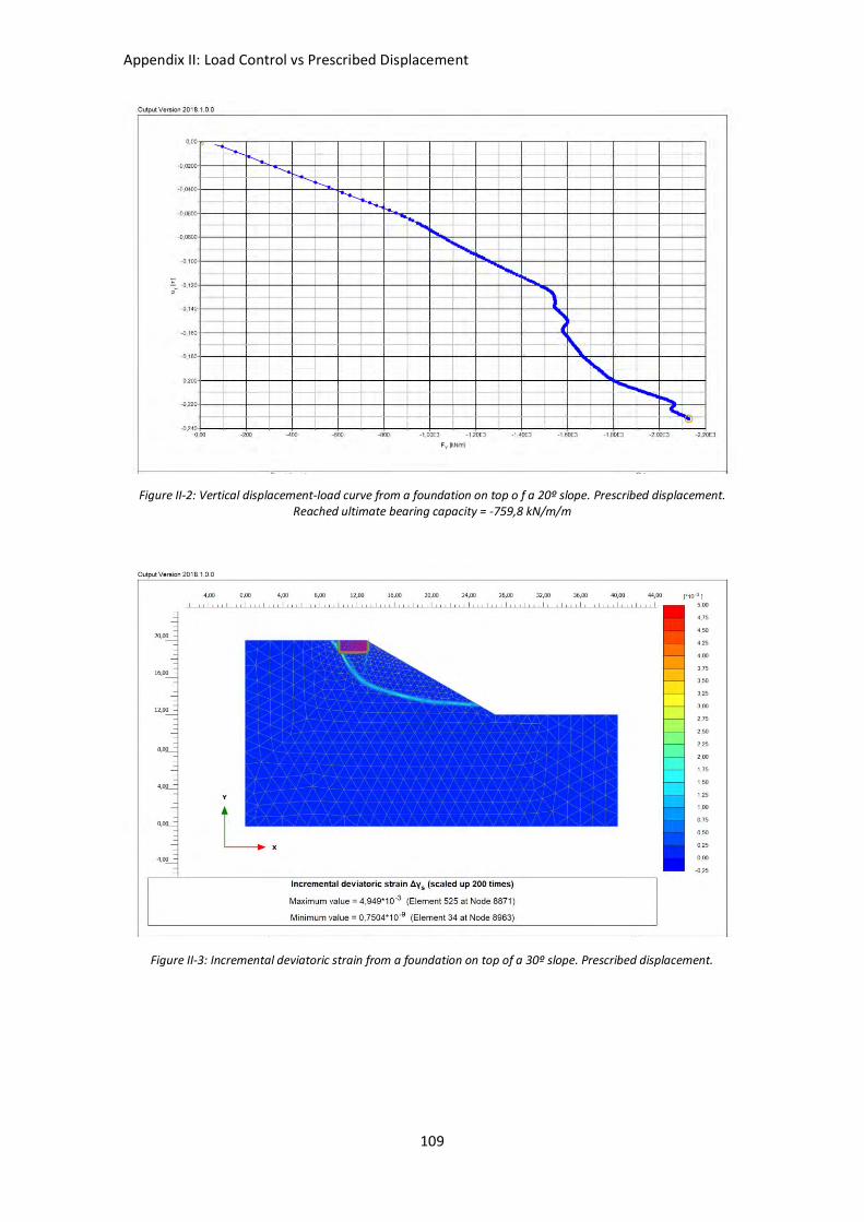
Appendix II: Load Control vs Prescribed Displacement
109
Figure II-2: Vertical displacement-load curve from a foundation on top o f a 20º slope. Prescribed displacement. Reached ultimate bearing capacity = -759,8 kN/m/m
Figure II-3: Incremental deviatoric strain from a foundation on top of a 30º slope. Prescribed displacement.

Appendix II: Load Control vs Prescribed Displacement
110
Figure II-4: Vertical displacement-load curve from a foundation on top of a 30º slope. Prescribed displacement. Reached maximum bearing capacity = -310 kN/m/m.
Figure II-5: Incremental deviatoric strain from a foundation in the middle of a 30º slope. Prescribed displacement.
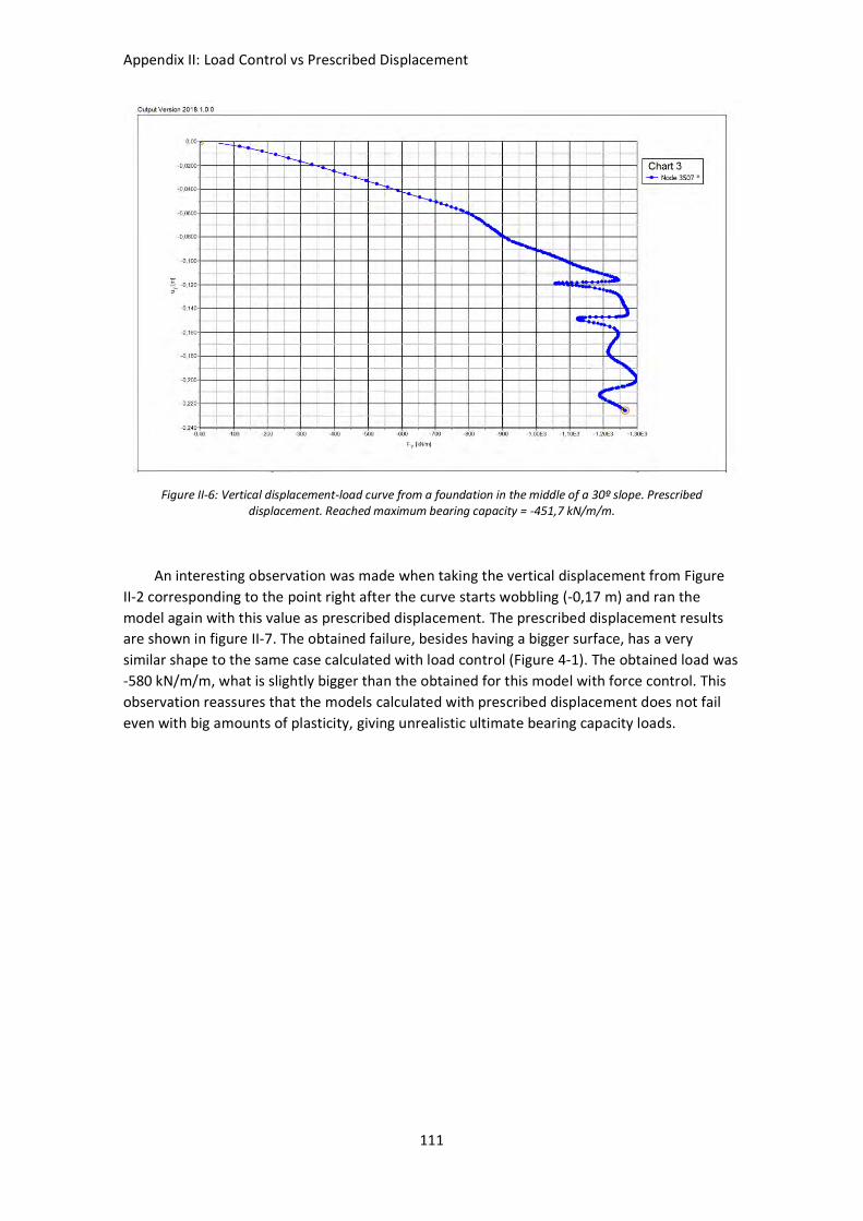
Appendix II: Load Control vs Prescribed Displacement
111
Figure II-6: Vertical displacement-load curve from a foundation in the middle of a 30º slope. Prescribed displacement. Reached maximum bearing capacity = -451,7 kN/m/m.
An interesting observation was made when taking the vertical displacement from Figure
II-2 corresponding to the point right after the curve starts wobbling (-0,17 m) and ran the
model again with this value as prescribed displacement. The prescribed displacement results
are shown in figure II-7. The obtained failure, besides having a bigger surface, has a very
similar shape to the same case calculated with load control (Figure 4-1). The obtained load was
-580 kN/m/m, what is slightly bigger than the obtained for this model with force control. This
observation reassures that the models calculated with prescribed displacement does not fail
even with big amounts of plasticity, giving unrealistic ultimate bearing capacity loads.

Appendix II: Load Control vs Prescribed Displacement
112
Figure II-7: Incremental displacemets from a foundation on top of a 20º slope. Prescribed displacement = -0,17 m
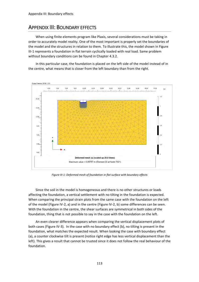
Appendix III: Boundary effects
113
APPENDIX III: BOUNDARY EFFECTS
When using finite elements program like Plaxis, several considerations must be taking in
order to accurately model reality. One of the most important is properly set the boundaries of
the model and the structures in relation to them. To illustrate this, the model shown in Figure
III-1 represents a foundation in flat terrain cyclically loaded with real load. Same problem
without boundary conditions can be found in Chapter 4.3.2.
In this particular case, the foundation is placed on the left side of the model instead of in
the centre, what means that is closer from the left boundary than from the right.
Figure III-1: Deformed mesh of foundation in flat surface with boundary effects
Since the soil in the model is homogeneous and there is no other structures or loads
affecting the foundation, a vertical settlement with no tilting in the foundation is expected.
When comparing the principal strain plots from the same case with the foundation on the left
of the model (Figure IV-2, a) and in the centre (Figure IV-2, b) some differences can be seen.
With the foundation in the centre, the shear surfaces are symmetrical in both sides of the
foundation, thing that is not possible to say in the case with the foundation on the left.
An even clearer difference appears when comparing the vertical displacement plots of
both cases (Figure IV-3). In the case with no boundary effect (b), no tilting is present in the
foundation, what matches the expected result. When looking the case with boundary effect
(a), a counter clockwise tilt is present (notice right edge has less vertical displacement than the
left). This gives a result that cannot be trusted since it does not follow the real behaviour of the
foundation.
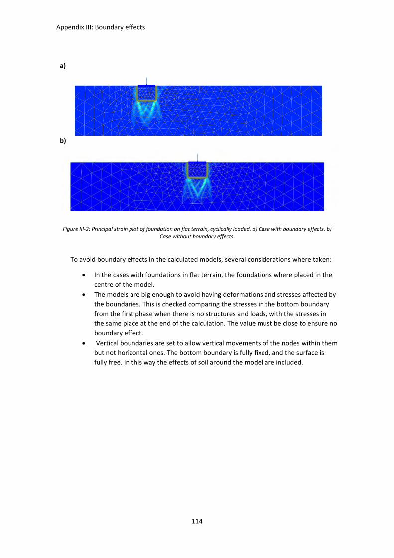
Appendix III: Boundary effects
114
a)
b)
Figure III-2: Principal strain plot of foundation on flat terrain, cyclically loaded. a) Case with boundary effects. b) Case without boundary effects.
To avoid boundary effects in the calculated models, several considerations where taken:
• In the cases with foundations in flat terrain, the foundations where placed in the
centre of the model.
• The models are big enough to avoid having deformations and stresses affected by
the boundaries. This is checked comparing the stresses in the bottom boundary
from the first phase when there is no structures and loads, with the stresses in
the same place at the end of the calculation. The value must be close to ensure no
boundary effect.
• Vertical boundaries are set to allow vertical movements of the nodes within them
but not horizontal ones. The bottom boundary is fully fixed, and the surface is
fully free. In this way the effects of soil around the model are included.

Appendix III: Boundary effects
115
a)
b)
Figure III-3: Vertical displacement of middle (blue), Left corner (red) and right corner (purple) of a foundation on flat terrain with cyclic loading. a) Case with boundary effects. b) Case without boundary effects.

Appendix IV: Ultimate Bearing Capacity, Shear Surfaces Development
116
APPENDIX IV: ULTIMATE BEARING CAPACITY, SHEAR SURFACES
DEVELOPMENT
In the present appendix, Figures complementing the ones located in Chapter 4.1.3 will be
gathered. For each ultimate bearing capacity calculation case, two more Figures will be shown
at different Mstages during loading: at Mstage = 0,5 (halve of the ultimate load) and Mstage =
0,75 (three fourths of the ultimate bearing capacity).
This is made for the sake of finding how the shear surfaces develop along the loading
process and have a better understanding of the failure mechanism.
The comments about these figures can be found in Chapter 4.1.3 in the analysis of the
cases which they correspond.
A) FOUNDATION ON TOP OF A 20º SLOPE, ORIGINAL GEOMETRY
Figure IV-1: Incremental deviatoric strain for a foundation on top of a 20º slope with original geometry. Mstage = 0,5.
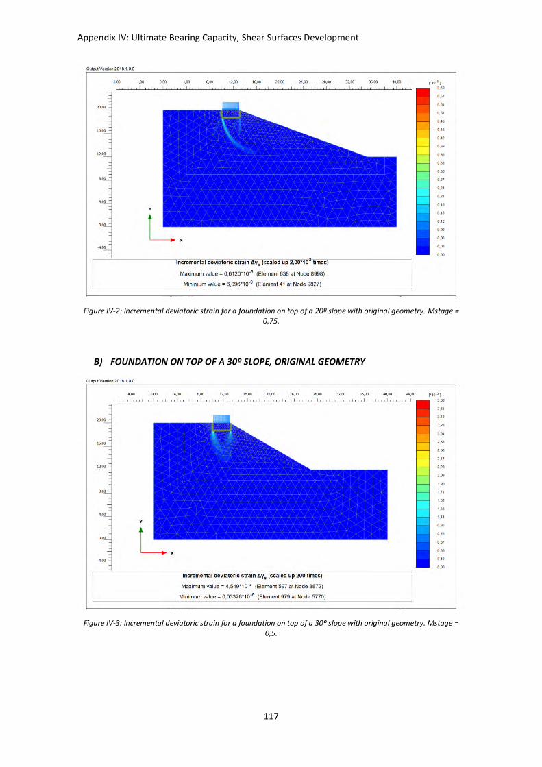
Appendix IV: Ultimate Bearing Capacity, Shear Surfaces Development
117
Figure IV-2: Incremental deviatoric strain for a foundation on top of a 20º slope with original geometry. Mstage = 0,75.
B) FOUNDATION ON TOP OF A 30º SLOPE, ORIGINAL GEOMETRY
Figure IV-3: Incremental deviatoric strain for a foundation on top of a 30º slope with original geometry. Mstage = 0,5.

Appendix IV: Ultimate Bearing Capacity, Shear Surfaces Development
118
Figure IV-4: Incremental deviatoric strain for a foundation on top of a 30º slope with original geometry. Mstage = 0,75.
C) FOUNDATION IN THE MIDDLE OF A 20º SLOPE, ORIGINAL GEOMETRY
Figure IV-5: Incremental deviatoric strain for a foundation in the middle of a 20º slope with original geometry. Mstage = 0,5.

Appendix IV: Ultimate Bearing Capacity, Shear Surfaces Development
119
Figure IV-6: Incremental deviatoric strain for a foundation in the middle of a 20º slope with original geometry. Mstage = 0,75.
D) FOUNDATION IN THE MIDDLE OF A 30º SLOPE, ORIGINAL GEOMETRY
Figure IV-7: Incremental deviatoric strain for a foundation in the middle of a 30º slope with original geometry. Mstage = 0,5.

Appendix IV: Ultimate Bearing Capacity, Shear Surfaces Development
120
Figure IV-8: Incremental deviatoric strain for a foundation in the middle of a 30º slope with original geometry. Mstage = 0,75.
E) FOUNDATION IN FLAT TERRAIN, ORIGINAL GEOMETRY
Figure IV -9: Incremental deviatoric strain for a foundation on flat terrain with original geometry. Mstage = 0,5.
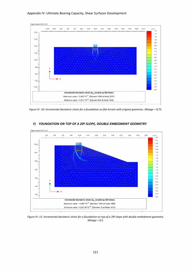
Appendix IV: Ultimate Bearing Capacity, Shear Surfaces Development
121
Figure IV -10: Incremental deviatoric strain for a foundation on flat terrain with original geometry. Mstage = 0,75.
F) FOUNDATION ON TOP OF A 20º SLOPE, DOUBLE EMBEDMENT GEOMETRY
Figure IV -11: Incremental deviatoric strain for a foundation on top of a 20º slope with double embedment geometry. Mstage = 0,5.
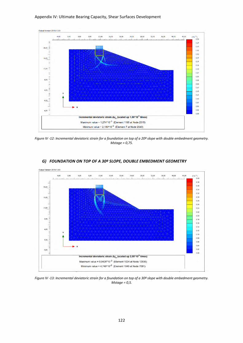
Appendix IV: Ultimate Bearing Capacity, Shear Surfaces Development
122
Figure IV -12: Incremental deviatoric strain for a foundation on top of a 20º slope with double embedment geometry. Mstage = 0,75.
G) FOUNDATION ON TOP OF A 30º SLOPE, DOUBLE EMBEDMENT GEOMETRY
Figure IV -13: Incremental deviatoric strain for a foundation on top of a 30º slope with double embedment geometry. Mstage = 0,5.
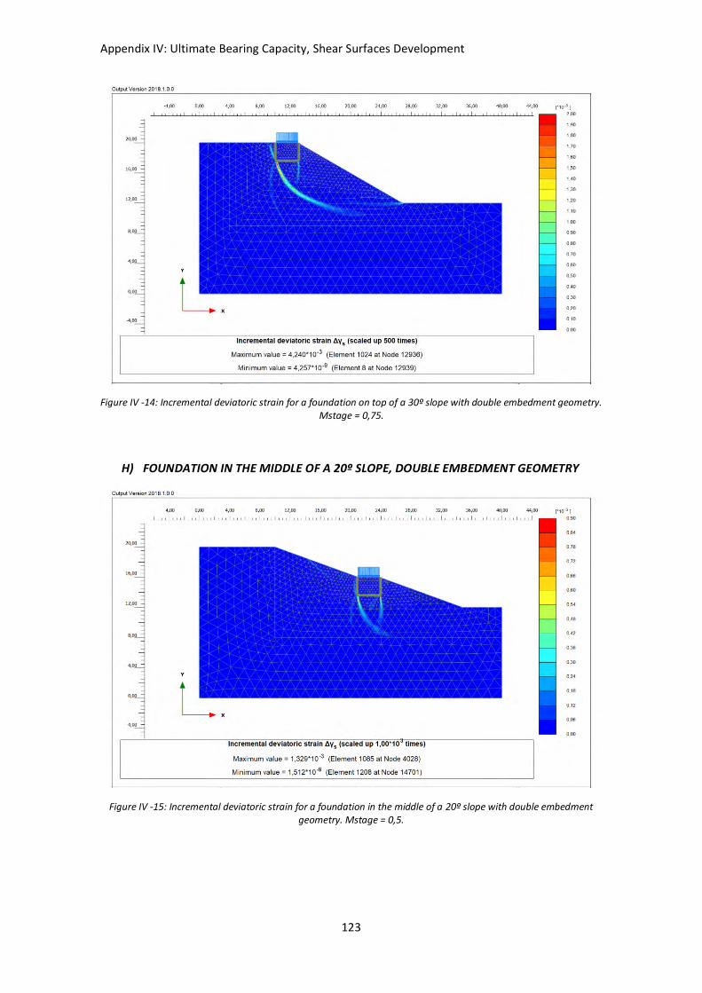
Appendix IV: Ultimate Bearing Capacity, Shear Surfaces Development
123
Figure IV -14: Incremental deviatoric strain for a foundation on top of a 30º slope with double embedment geometry. Mstage = 0,75.
H) FOUNDATION IN THE MIDDLE OF A 20º SLOPE, DOUBLE EMBEDMENT GEOMETRY
Figure IV -15: Incremental deviatoric strain for a foundation in the middle of a 20º slope with double embedment geometry. Mstage = 0,5.

Appendix IV: Ultimate Bearing Capacity, Shear Surfaces Development
124
Figure IV -16: Incremental deviatoric strain for a foundation in the middle of a 20º slope with double embedment geometry. Mstage = 0,75.
I) FOUNDATION IN THE MIDDLE OF A 30º SLOPE, DOUBLE EMBEDMENT GEOMETRY
Figure IV -17: Incremental deviatoric strain for a foundation in the middle of a 30º slope with double embedment geometry. Mstage = 0,5.

Appendix IV: Ultimate Bearing Capacity, Shear Surfaces Development
125
Figure IV -18: Incremental deviatoric strain for a foundation in the middle of a 30º slope with double embedment geometry. Mstage = 0,75.
J) FOUNDATION ON FLAT TERRAIN, DOUBLE EMBEDMENT GEOMETRY
Figure IV -19: Incremental deviatoric strain for a foundation on flat terrain with double embedment geometry. Mstage = 0,5.

Appendix IV: Ultimate Bearing Capacity, Shear Surfaces Development
126
Figure IV -20: Incremental deviatoric strain for a foundation on flat terrain with double embedment geometry. Mstage = 0,75.