Bearing capacity of a sand layer on clay by finite element ... · Bearing capacity of a sand layer on clay by finite element limit analysis J.S. Shiau, A.V. Lyamin, and S.W. Sloan

Bearing capacity of a sand layer on clay by finiteelement limit analysis

J.S. Shiau, A.V. Lyamin, and S.W. Sloan

Abstract: Rigorous plasticity solutions for the ultimate bearing capacity of a strip footing resting on a sand layer overclay soil are obtained by applying advanced upper and lower bound techniques. The study compares these solutionswith other published results and investigates the effect of various strength and geometry parameters. Assuming the soillayers obey an associated flow rule, the results presented typically bound the collapse load to within ±10% or better.

Key words: limit analysis, bearing capacity, layered soils, finite elements.

Résumé : On a obtenu des solutions rigoureuses en plasticité pour la capacité portante ultime d’une semelle filante surune couche de sable reposant sur un sol argileux en utilisant les techniques avancées de la limite supérieure et infé-rieure. L’étude compare ces solutions avec d’autres résultats publiés et examine l’effet de différents paramètres de ré-sistance et de géométrie. En supposant que les couches de sol obéissent à une loi d’écoulement associé, les résultatsont présenté la charge de rupture typiquement limitée à l’intérieur de ±10 % ou mieux.

Mots clés : analyse limite, capacité cortante, sols en couches, éléments finis.

[Traduit par la Rédaction] Shiau et al. 915

Introduction

The need to determine the bearing capacity of a com-pacted sand or gravel layer on soft clay arises frequently infoundation engineering. Of the published approaches to thisproblem, the semi-empirical solutions of Meyerhof (1974)and Hanna and Meyerhof (1980) are perhaps the mostwidely used in practice. Their methods are also known aspunching shear models, as they assume the sand layer to bein a state of passive failure along vertical planes beneath thefooting edges. Another commonly used semi-empirical ap-proach is the load spread model, in which the sand layer isassumed to merely spread the load to the underlying clayfoundation (e.g., Terzaghi and Peck 1948; Houlsby et al.1989). This technique ignores the shear strength of the sandand transforms the problem to the classical one of estimatingthe bearing capacity of a clay layer that is subjected to a sur-charge.

A more rigorous approach, based on the upper bound the-orem of limit analysis, has been used by Chen and Davidson(1973), Florkiewicz (1989), and Michalowski and Shi (1995)to calculate the bearing capacity of multilayered soils. Thesestudies consider various rigid block mechanisms that, at thepoint of collapse, assume power is dissipated solely at theinterfaces between adjacent blocks. After optimizing the ge-ometry to furnish the minimum dissipated power, the mecha-

nism that gives the lowest value is used to compute the bestupper bound on the limit load. To give confidence in the ac-curacy of the solutions obtained from upper bound calcula-tions, it is desirable to perform lower bound calculations inparallel so that the true result can be bracketed from aboveand below (Davis 1968; Chen 1975; Sloan 1988, 1989). Un-fortunately, due to the difficulty in constructing staticallyadmissible stress fields by traditional methods, this is rarelydone in practice.

Although conventional finite element analysis can be usedto predict the bearing capacity of multilayered soils(Griffiths 1982; Burd and Frydman 1997), the estimate soobtained is neither an upper bound nor a lower bound on thetrue value. Moreover, great care needs to be exercised withdisplacement finite element predictions in the fully plasticrange, as the results can be very inaccurate due to the occur-rence of locking (Nagtegaal et al. 1974; Sloan and Randolph1982). This phenomenon, which is characterized by a con-stantly rising load–deformation response, occurs when thedisplacement field becomes overconstrained by the require-ments of an incompressible plastic flow rule. To estimateundrained limit loads accurately using displacement finiteelements in plane strain, it is prudent to avoid using low-order formulations (Sloan and Randolph 1982) unless theyare used with some form of selective integration (Nagtegaalet al. 1974).

In this paper, we use finite element formulations of thelimit analysis theorems to obtain rigorous plasticity solutionsfor the bearing capacity of a layer of sand on clay. FollowingMerifield et al. (1999), who considered the classical bearingcapacity problem of a two-layered clay, we use the boundingmethods to bracket the true solution from above and below.The techniques themselves have been developed only re-cently and are discussed in detail by Lyamin and Sloan

Can. Geotech. J. 40: 900–915 (2003) doi: 10.1139/T03-042 © 2003 NRC Canada

900

Received 30 April 2002. Accepted 10 April 2003. Publishedon the NRC Research Press Web site at http://cgj.nrc.ca on8 September 2003.

J.S. Shiau, A.V. Lyamin, and S.W. Sloan.1 Civil, Surveyingand Environmental Engineering, University of Newcastle,Callaghan, NSW 2308, Australia.

1Corresponding author (e-mail: [email protected]).

I:\cgj\CGJ40-05\T03-042.vpSeptember 3, 2003 1:47:23 PM

Color profile: DisabledComposite Default screen

(2002a, 2002b). These procedures effectively supersede theearlier formulations proposed by Sloan (1988, 1989) andSloan and Kleeman (1995) which, although successful in awide range of practical applications, are less efficient.

Problem definition

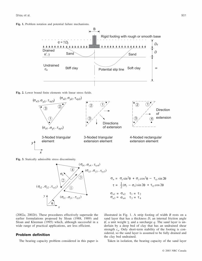
The bearing capacity problem considered in this paper is

illustrated in Fig. 1. A strip footing of width B rests on asand layer that has a thickness D, an internal friction angleφ′, a unit weight γ, and a surcharge q. The sand layer is un-derlain by a deep bed of clay that has an undrained shearstrength cu. Only short-term stability of the footing is con-sidered, so the sand layer is assumed to be fully drained andthe clay bed undrained.

Taken in isolation, the bearing capacity of the sand layer

© 2003 NRC Canada

Shiau et al. 901

Fig. 1. Problem notation and potential failure mechanisms.

Fig. 2. Lower bound finite elements with linear stress fields.

Fig. 3. Statically admissible stress discontinuity.



© 2003 NRC Canada

902 Can. Geotech. J. Vol. 40, 2003

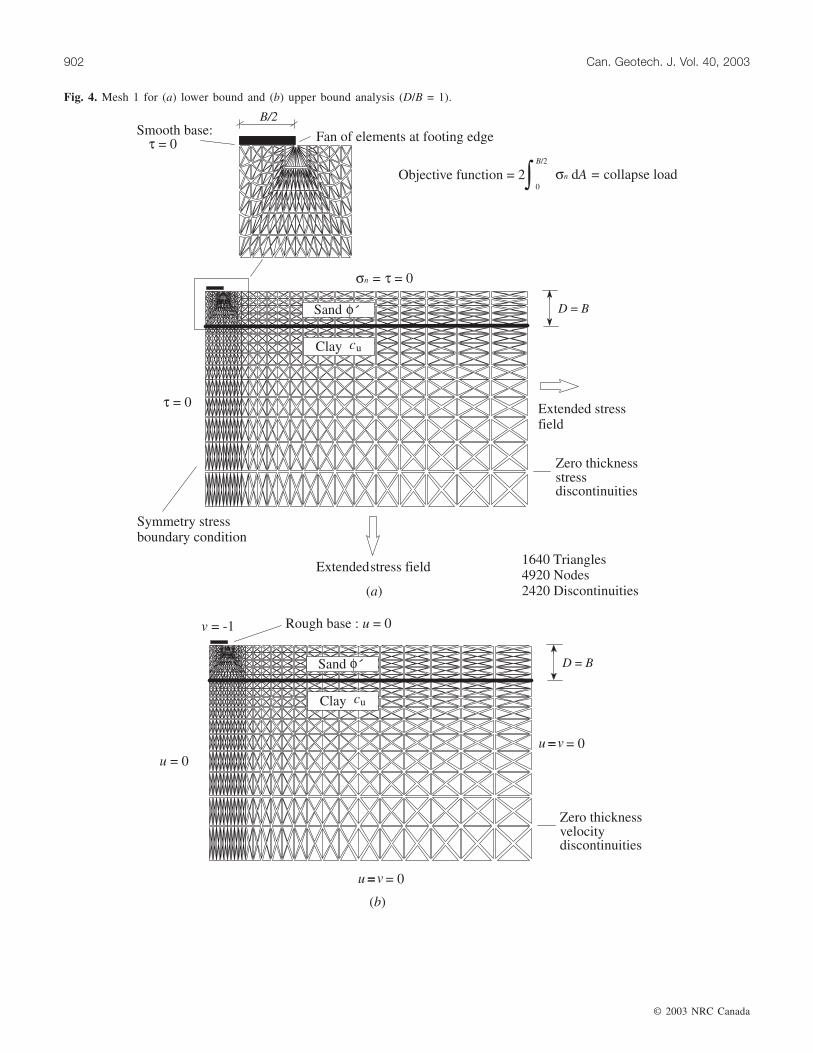
Fig. 4. Mesh 1 for (a) lower bound and (b) upper bound analysis (D/B = 1).



will be governed by φ′, γ, and q, with other possible factorsbeing the dilation angle ψ′ and the footing roughness. Classi-cal limit analysis theory assumes an associated flow rule,where normality of the plastic strains to the yield functionapplies and the dilation angle is set equal to the friction an-gle. Allowing for the presence of the clay layer, and assum-ing associated flow with a perfectly rough footing, theultimate bearing capacity of the two-layer foundation prob-lem can be expressed in the dimensionless form

[1]pB

fDB

cB

qBγ γ γ

φ= ′

, , ,u

where p is the average limit pressure. Accordingly, in thefollowing, the bearing capacities are presented in terms ofthe dimensionless quantities D/B, cu/γB, q/γB, and φ′, withthe role of the dilation angle and footing roughness investi-gated separately.

Numerical limit analysis models

This section gives a very brief summary of the finite ele-ment formulations of the upper and lower bound theorems.A more detailed description of the techniques, including adiscussion of the solution algorithms used to solve the re-sulting optimization problem, can be found in Lyamin andSloan (2002a, 2002b) and will not be repeated here.

The lower bound limit theorem states that if any equilib-rium state of stress can be found which balances the appliedloads and satisfies the yield criterion as well as the stressboundary conditions, then the body will not collapse (Chen1975). Stress fields that satisfy these requirements, and thusgive lower bounds, are said to be statically admissible. Thekey idea behind the lower bound analysis applied here is tomodel the stress field using finite elements and use the staticadmissibility constraints to express the unknown collapseload as a solution to a mathematical programming problem.For linear elements, the equilibrium and stress boundaryconditions give rise to linear equality constraints on thenodal stresses, and the yield condition, which requires allstress points to lie inside or on the yield surface, gives riseto a nonlinear inequality constraint on each set of nodalstresses. The objective function, which is to be maximized,corresponds to the collapse load and is a function of the un-

known stresses. For linear elements, this function is also lin-ear. After all the element coefficients are assembled, the fi-nal optimization problem is thus one with a linear objectivefunction, linear equality constraints, and nonlinear inequalityconstraints.

The lower bound formulation proposed by Lyamin andSloan (2002a) handles both two- and three-dimensionalstress fields and, in the former case, employs the linear ele-ments shown in Fig. 2. Note that it incorporates staticallyadmissible stress discontinuities at all interelement bound-aries (Fig. 3) and special extension elements for completingthe stress field in an unbounded domain (Fig. 2). Unlike dis-placement finite element meshes, each node is unique to asingle element and several nodes may share the same coordi-nates. Although the stress discontinuities increase the totalnumber of variables for a fixed mesh, they also introduce ex-tra “degrees of freedom” in the stress field, thus improvingthe accuracy of the solution. Along a given discontinuity thenormal and shear stresses must be continuous, but the tan-gential normal stress may be discontinuous.

As the formulation of Lyamin and Sloan (2002a) uses lin-ear elements in both two and three dimensions, the objectivefunction and equality constraints are linear in the unknowns.As discussed previously, the equality constraints arisebecause the stress field needs to satisfy equilibrium in thecontinuum and the discontinuities, as well as the stressboundary conditions. Some additional constraints may alsobe required to incorporate special types of loading along thedomain boundaries. After assembling the various objectivefunction coefficients and equality constraints for the mesh,and imposing the nonlinear yield inequalities on each node,the lower bound formulation of Lyamin and Sloan leads to anonlinear programming problem of the form

[2]

max

( ) {, ... }

imize

subject to =

Tc

A b

�

�

�f i Ni ≤ =0 1

where c is a vector of objective function coefficients, � is avector of unknowns (nodal stresses and possibly elementunit weights), cT� is the collapse load, A is a matrix ofequality constraint coefficients, b is a vector of coefficients,fi is the yield function for node i, and N is the number ofnodes. The solution to eq. [2], which constitutes a staticallyadmissible stress field, can be found efficiently by solvingthe system of nonlinear equations that define its Kuhn-Tucker optimality conditions. Indeed, the two-stage quasi-Newton solver developed by Lyamin (1999) usually needsfewer than about 50 iterations, regardless of the problemsize. Because it does not require the yield surface to belinearized, the formulation can be used for a wide range ofconvex yield criteria.

A “fan” mesh for a lower bound analysis of the problemdefined in Fig. 1 is shown in Fig. 4a. The grid consists of4920 nodes, 1640 triangular elements, and 2420 stress dis-continuities. It includes special extension elements along thebottom and right boundaries (not shown for clarity) to ex-tend the stress field throughout the semi-infinite domain.The fan of elements centred on the footing edge permits theprincipal stresses to rotate around this point and improves

© 2003 NRC Canada

Shiau et al. 903

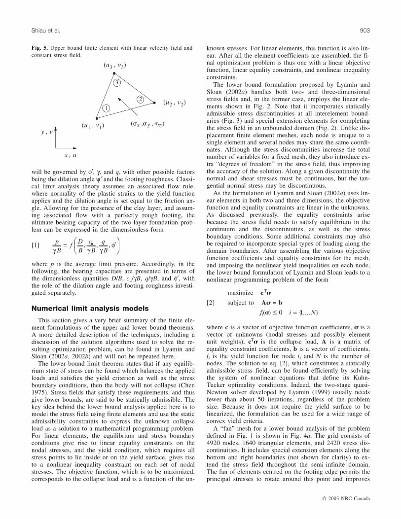
Fig. 5. Upper bound finite element with linear velocity field andconstant stress field.



the accuracy of the lower bound. This aspect and the resultsfrom an alternative type of mesh are investigated in a latersection of the paper.

To model a smooth footing that has no shear stress on itsunderside, additional constraints have to be imposed at allelement nodes along the footing–soil interface. For a roughfooting, the shear stress is typically nonzero and governedsolely by the specified yield criterion.

The upper bound theorem can be formulated in terms offinite elements by adopting a similar approach to that justdescribed for the static case. This theorem states that thepower dissipated by any kinematically admissible velocityfield can be equated to the power dissipated by the externalloads to give a rigorous upper bound on the true limit load.A kinematically admissible velocity field is one that satisfiescompatibility, the flow rule, and the velocity boundary con-ditions. In a finite element formulation of the upper boundtheorem, the velocity field is modelled using appropriatevariables, and the optimum (minimum) internal power dissi-pation is obtained as the solution to a mathematical pro-gramming problem.

© 2003 NRC Canada


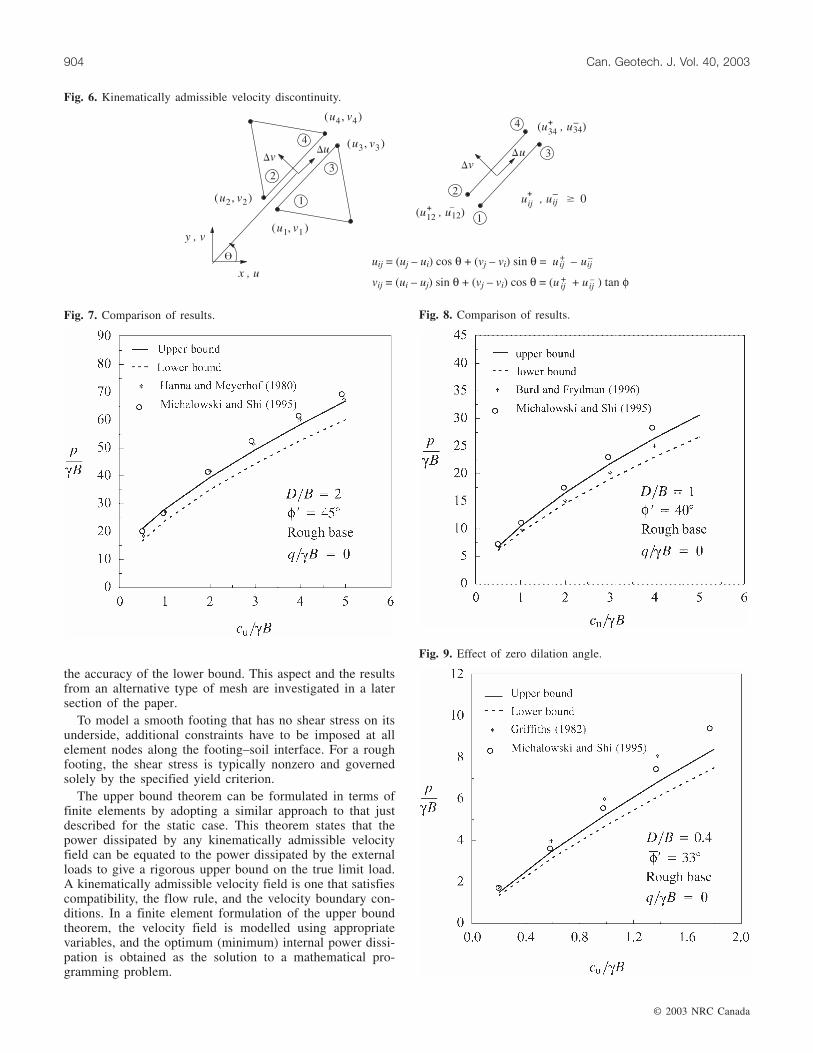
Fig. 6. Kinematically admissible velocity discontinuity.

Fig. 7. Comparison of results. Fig. 8. Comparison of results.

Fig. 9. Effect of zero dilation angle.



In the formulation of Lyamin and Sloan (2002b), theupper bound is found by the solution of a nonlinear pro-gramming problem. Their procedure uses linear triangles tomodel the velocity field, and each element is also associatedwith a constant stress field and a single plastic multiplierrate (Fig. 5). The element plastic multipliers do not need tobe included explicitly as variables, however, even thoughthey are used in the derivation of the formulation. This is be-

cause the final optimization problem can be cast in terms ofthe nodal velocities and element stresses alone. To ensurekinematic admissibility, flow-rule constraints are imposedon the nodal velocities, element plastic multipliers, and ele-ment stresses. In addition, the velocities are matched to thespecified boundary conditions, the plastic multipliers areconstrained to be non-negative, and the element stresses areconstrained to satisfy the yield criterion. Following Sloan

© 2003 NRC Canada

Shiau et al. 905

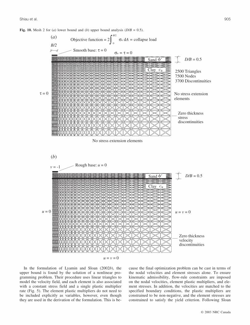
Fig. 10. Mesh 2 for (a) lower bound and (b) upper bound analysis (D/B = 0.5).



© 2003 NRC Canada


p/γB

Mesh 1 (Fig. 4) Mesh 2 (Fig. 10)

cu/γBLower bound(LB)

Upper bound(UB)

Accuracy(%)a

Lowerbound (LB)

Upper bound(UB)

Accuracy(%)a

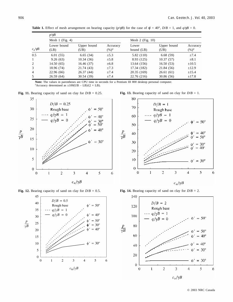
0.5 6.01 (55) 6.65 (34) ±5.3 5.82 (110) 6.68 (59) ±7.41 9.26 (63) 10.34 (36) ±5.8 8.93 (125) 10.37 (57) ±8.12 14.50 (65) 16.46 (37) ±6.8 13.64 (156) 16.50 (53) ±10.53 18.96 (74) 21.74 (43) ±7.3 17.34 (182) 21.84 (56) ±12.94 22.96 (66) 26.37 (44) ±7.4 20.35 (169) 26.61 (61) ±15.45 26.59 (64) 30.54 (39) ±7.4 22.76 (216) 30.86 (56) ±17.8

Note: The values in parentheses are CPU time in seconds for a Pentium III 800 desktop personal computer.aAccuracy determined as ±100(UB – LB)/(2 × LB).

Table 1. Effect of mesh arrangement on bearing capacity (p/γB) for the case of φ′ = 40°, D/B = 1, and q/γB = 0.

Fig. 11. Bearing capacity of sand on clay for D/B = 0.25. Fig. 13. Bearing capacity of sand on clay for D/B = 1.

Fig. 12. Bearing capacity of sand on clay for D/B = 0.5. Fig. 14. Bearing capacity of sand on clay for D/B = 2.



and Kleeman (1995), the method of Lyamin and Sloan per-mits velocity discontinuities at all interelement boundaries inthe mesh. As shown in Fig. 6, each discontinuity is definedby four nodes and requires four unknowns to describe thevelocity jumps along its length.

With the elements shown in Figs. 5 and 6, plastic defor-mation can occur in both the continuum and the velocity dis-

continuities, giving rise to two different sources of powerdissipation. For a given set of prescribed velocities, the fi-nite element formulation works by choosing the set of veloc-ities and stresses that minimize the dissipated power. Thispower is then equated to the power dissipated by the exter-nal loads to yield a strict upper bound on the true limit load.

After assembling the various objective function coeffi-

© 2003 NRC Canada

Shiau et al. 907

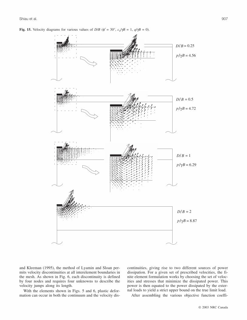
Fig. 15. Velocity diagrams for various values of D/B (φ′ = 30°, cu/γB = 1, q/γB = 0).



cients and constraints for the mesh, the upper bound formu-lation of Lyamin and Sloan (2002b) leads to a nonlinearprogramming problem of the form

Minimize �TuT

dTBu c c d+ + on (u,d)

Subject to A u A du d+ = b

[3] Bu = λ i ii

E

f∇=∑ ( )�

1

λ i ≥ 0 i = {1,...E}

λ i if ( )� = 0 i = {1,...E}

fi( )� ≤ 0 i = {1,...E}

d ≥ 0

where u is a global vector of unknown velocities; d is aglobal vector of unknown discontinuity variables; � is aglobal vector of unknown element stresses; cu and cd arevectors of objective function coefficients for the nodal veloc-ities and discontinuity variables, respectively; Au and Ad arematrices of equality constraint coefficients for the nodalvelocities and discontinuity variables, respectively; B isa global matrix of compatibility coefficients that operateon the nodal velocities; b is a vector of coefficients; ∇ = {∂/∂σx, ∂/∂σy, ∂/∂ τxy}

T; λi is an unknown plastic multiplier ratefor element i; fi is the yield function for element i; and E isthe number of triangular elements. In this equation, the ob-jective function �TBu + cu

Tu + cdTd denotes the total dissi-

pated power, with the first term giving the dissipation in thecontinuum, the second term giving the dissipation becauseof fixed boundary tractions or body forces, and the thirdterm giving the dissipation in the discontinuities. Using its

© 2003 NRC Canada


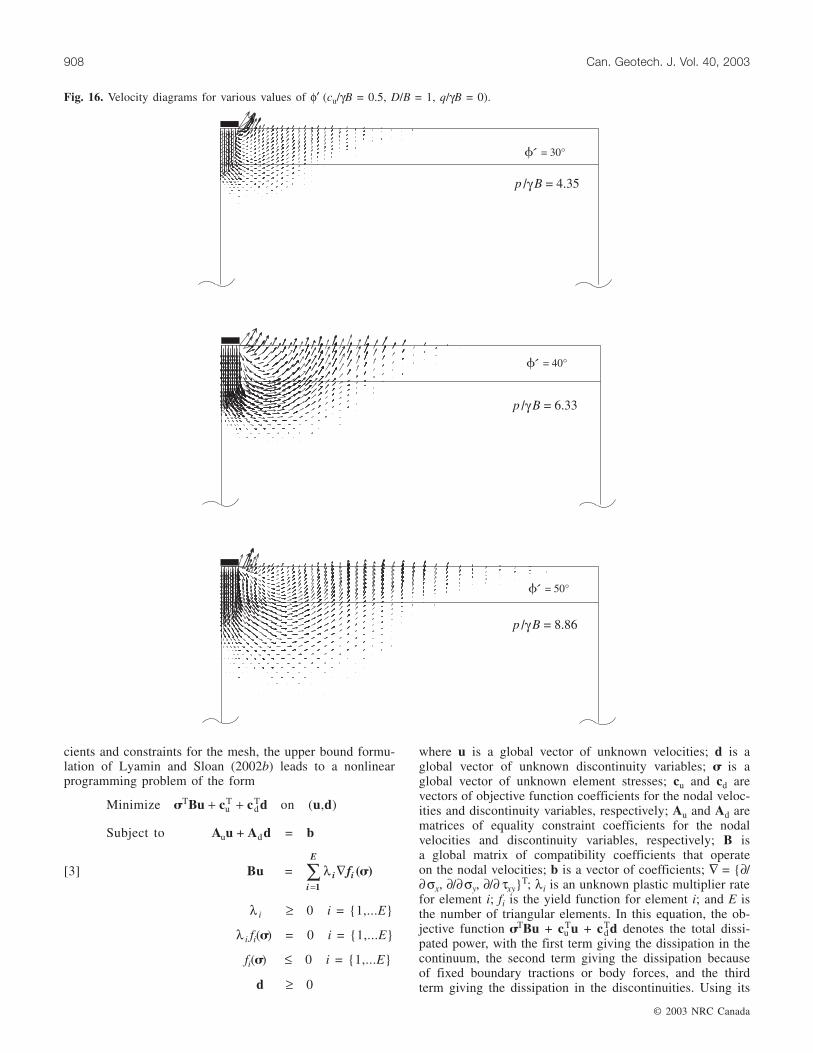
Fig. 16. Velocity diagrams for various values of φ′ (cu/γB = 0.5, D/B = 1, q/γB = 0).



Kuhn-Tucker optimality conditions, the optimization prob-lem (eq. [3]) may be recast in the alternative form

Maximize �TuT

dTBu c u c d+ + on (�)

Minimize �TuT

dTBu c u c d+ + on (u,d)

[4] Subject to A u A du d+ = b

fi( )� ≤ 0 i = {1,...E}

d ≥ 0

which has fewer variables (the plastic multipliers are no lon-ger needed) and fewer constraints. The solution to eq. [4]can be computed efficiently using a two-stage quasi-Newtonsolver which is a variant of the scheme developed for thelower bound method (Lyamin and Sloan 2002b). Again, amaximum of 50 iterations is typically required, regardless ofthe problem size.

Figure 4b shows a fan-type mesh for upper bound limitanalysis of the problem considered. This mesh is identical tothe lower bound mesh in Fig. 4a, except it does not need toincorporate extension elements along the bottom and rightboundaries. An upper bound solution is obtained by pre-scribing a unit downward velocity to the nodes on the foot-ing. To model a perfectly rough foundation, these nodes areconstrained so that they cannot move horizontally (u = 0).After the resulting optimization problem is solved for theimposed boundary conditions, the upper bound on the col-lapse load is obtained by equating the power expended bythe external loads to the power dissipated internally by plas-tic deformation.

Results and discussion

Using the methods described in the previous section, finiteelement limit analyses were performed to obtain upper and

© 2003 NRC Canada

Shiau et al. 909

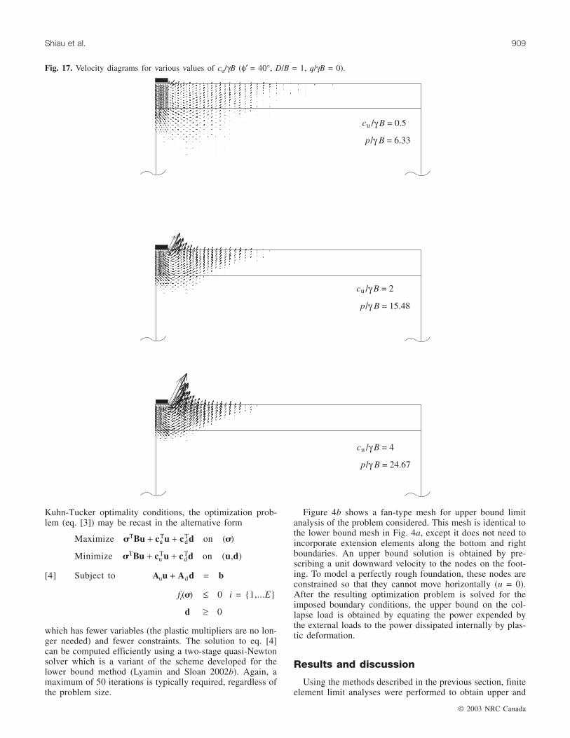
Fig. 17. Velocity diagrams for various values of cu/γB (φ′ = 40°, D/B = 1, q/γB = 0).



lower bound bearing capacity estimates for strip footings onvarious sand and clay layers. The study assumes the soil lay-ers obey an associated flow rule and covers a range of pa-rameters, including the depth of the sand layer (D/B), thefriction angle of the sand (φ′), the undrained shear strengthof the clay (cu/γB), and the effect of a surcharge (q/γB). Theinfluence of footing roughness and increasing strength withdepth for the clay soil are also quantified rigorously. For asingle example, the effect of zero dilatancy in the sand layeris investigated approximately by using an associated flowrule with a reduced friction angle. Where possible, the newnumerical results are compared with solutions obtained byothers.

Comparisons with previous resultsThe lower and upper bound estimates of the normalized

bearing capacity p/γB are compared with the semi-empirical

results suggested by Hanna and Meyerhof (1980), the dis-placement finite element method solutions of Griffiths(1982) and Burd and Frydman (1996), and the analytical ki-nematic predictions of Michalowski and Shi (1995). Thesecomparisons are shown in Figs. 7–9. The lower and upperbounds were computed using meshes similar to those inFig. 4.

For the case of φ′ = 45°, D/B = 2, and q/γB = 0, Fig. 7shows that the semi-empirical approach of Hanna andMeyerhof (1980) and the analytical kinematic approach ofMichalowski and Shi (1995) both overestimate the bearingcapacity p/γB at larger values of cu/γB. Although their solu-tions are reasonably close to our upper bounds, they are upto 18% above our lower bounds. As shown in Fig. 8, the ki-nematic results of Michalowski and Shi display similartrends for the case of φ′ = 40°, D/B = 1, and q/γB = 0. Thenumerical results reported by Burd and Frydman (1996),

© 2003 NRC Canada


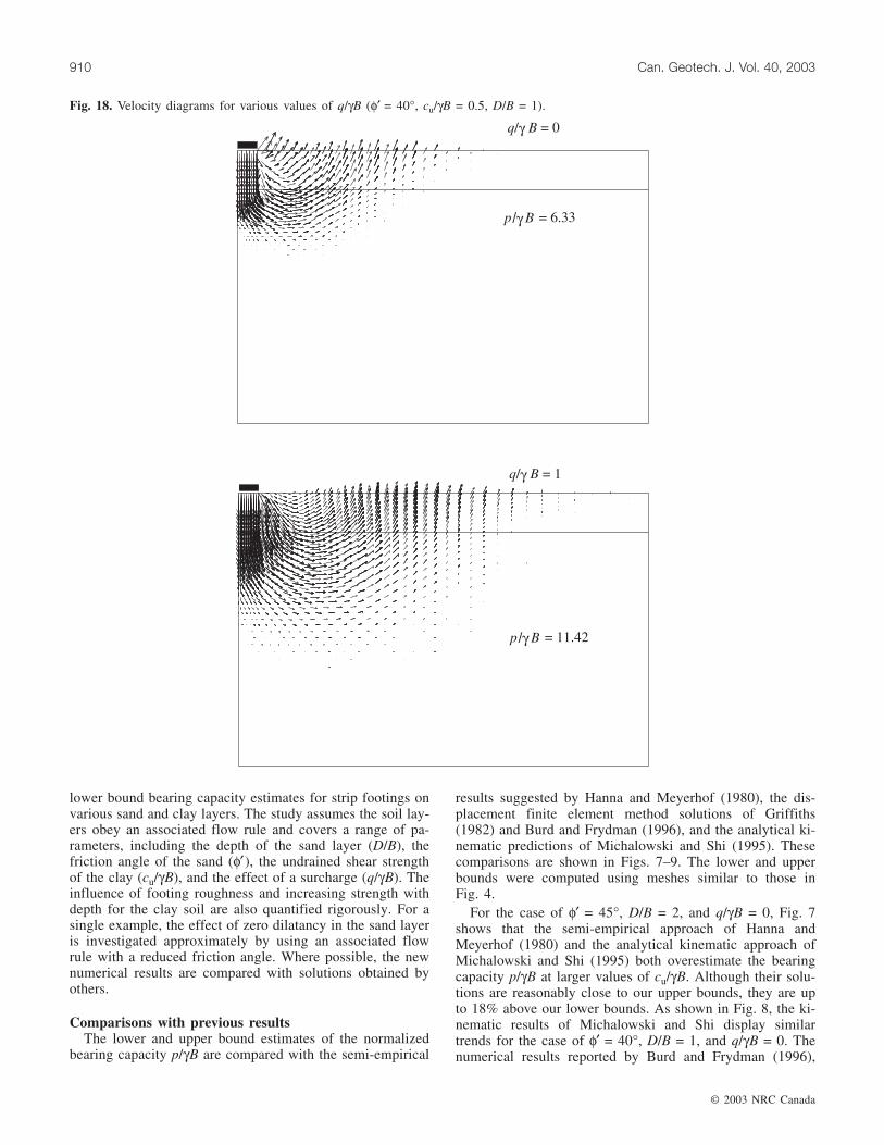
Fig. 18. Velocity diagrams for various values of q/γB (φ′ = 40°, cu/γB = 0.5, D/B = 1).



also plotted in Fig. 8, are for a non-associated flow rule witha dilation angle of ψ′ = 10° and represent average values ob-tained from their displacement finite element and finite dif-ference analyses. Their bearing capacity predictions lie closeto the average of our upper and lower bound estimates.

To compare their kinematic results with those of Griffiths(1982), who employed the displacement finite elementmethod with a non-associated flow rule for the sand layer,Michalowski and Shi (1995) replace the sand friction angleφ′ by ′φ , where

[5] tancos cos

sin sintan′ = ′ ′

− ′ ′′φ ψ φ

ψ φφ

1

This follows the work of Drescher and Detournay (1993)who argue that, for kinematic mechanisms comprised solelyof rigid blocks and velocity discontinuities, the use of ′φ in-stead of φ′ will furnish reasonable limit load estimates formaterials with coaxial non-associated flow rules. Indeed,Drescher and Detournay suggest that ′φ may be viewed as a“residual” friction angle which accounts for the softeningthat may be induced under certain stress conditions by anon-associated flow rule. Because failure may occur beforeall the stresses reach the residual state, this approach maygive limit loads that are lower than the true values. Figure 9compares the solutions of Griffiths (1982) and Michalowskiand Shi (1995) with our bound solutions for ′φ = 33°, whichapproximates the non-associated zero dilation case whereφ′ = 40° and ψ′ = 0°. Since our upper bound method permitsplastic dissipation in both the continuum and the velocitydiscontinuities, and thus violates one of the conditions of theproof by Drescher and Detournay, these results should betreated with some caution. Bearing this in mind, the predic-tions of Griffiths and Michalowski and Shi are reasonablyclose to our bound solutions for small to medium values ofcu/γB, but give higher bearing capacities as cu/γB increases.

Because of the large volume changes they predict duringplastic shearing, associated flow rules are sometimes thoughtto give questionable limit loads for frictional soils. For caseswhere the failure mechanism is kinematically highly con-strained, such as granular flow in a hopper, this concern iscertainly valid and needs to be addressed. For frictional soilswith a freely deforming surface and a semi-infinite domain,however, the use of an associated flow rule will, in manycases, give good estimates of the collapse load. Althoughdifficult to quantify, this important result is discussed atlength in Davis (1968) and has been confirmed by a numberof independent finite element studies (e.g., Zienkiewicz et al.1975; Sloan 1981).

Overall, the results shown in Figs. 7–9 suggest that thenew bound solutions give bearing capacities which are moreconservative than those published previously. Assuming thesoil layers obey an associated flow rule, the finite elementlimit analyses typically bound the limit load to ±10% orbetter.

Effect of mesh arrangementFor the case of φ′ = 40°, D/B = 1, and q/γB = 0, Table 1

compares the results from two different types of mesh ar-rangement with the upper and lower bound analyses. Closebounds are always obtained using mesh type 1 (Fig. 4),which has a fan of discontinuities at the footing edge. Theresults from mesh type 2 (Fig. 10) are less satisfactory, withthe accuracy of the lower bounds decreasing as cu/γB in-creases. Solutions from this type of grid cannot be improvedby using additional elements, as it will always fail to modelthe principal stress rotation at the edge of the footingadequately. Interestingly, the accuracy of the upper boundsolutions is roughly the same for both types of mesh ar-rangement. All subsequent limit analysis results in this paperwere obtained using fan-type meshes similar to those inFig. 4.

The central processing unit (CPU) times in Table 1 showthat the finite element bound formulations of Lyamin andSloan (2002a, 2002b) are computationally very efficient. Toobtain solutions of roughly the same accuracy using the con-ventional displacement method would, in the authors’ expe-rience, require similar computational effort. For materialswith an associated flow rule, the limit analysis solutionshave the key advantage of an built-in error indicator, withthe lower bounds always providing a conservative estimateof the bearing capacity. They also furnish the limit load di-rectly, without the need to infer it from a load–deformationresponse.

Parametric studyAssuming an associated flow rule for the soil layers,

Figs. 11–14 present results for the normalized bearing ca-pacity p/γB as a function of the dimensionless quantitiesD/B, cu/γB, q/γB, and φ′. These plots are for φ′ = 30°, 40°,and 50°, q/γB = 0 and 1, and D/B = 0.25, 0.5, 1, and 2 andare averages of the upper and lower bound estimates for thecase of a perfectly rough footing. In all cases the spread ofthe bound solutions is less than ±10%, which is sufficientlyaccurate for the purposes of design.

© 2003 NRC Canada

Shiau et al. 911

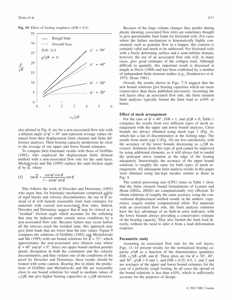
Fig. 19. Effect of footing roughness (D/B = 0.5).



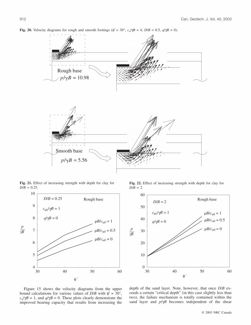
Figure 15 shows the velocity diagrams from the upperbound calculations for various values of D/B with φ′ = 30°,cu/γB = 1, and q/γB = 0. These plots clearly demonstrate theimproved bearing capacity that results from increasing the

depth of the sand layer. Note, however, that once D/B ex-ceeds a certain “critical depth” (in this case slightly less thantwo), the failure mechanism is totally contained within thesand layer and p/γB becomes independent of the shear

© 2003 NRC Canada


Fig. 20. Velocity diagrams for rough and smooth footings (φ′ = 30°, cu/γB = 4, D/B = 0.5, q/γB = 0).

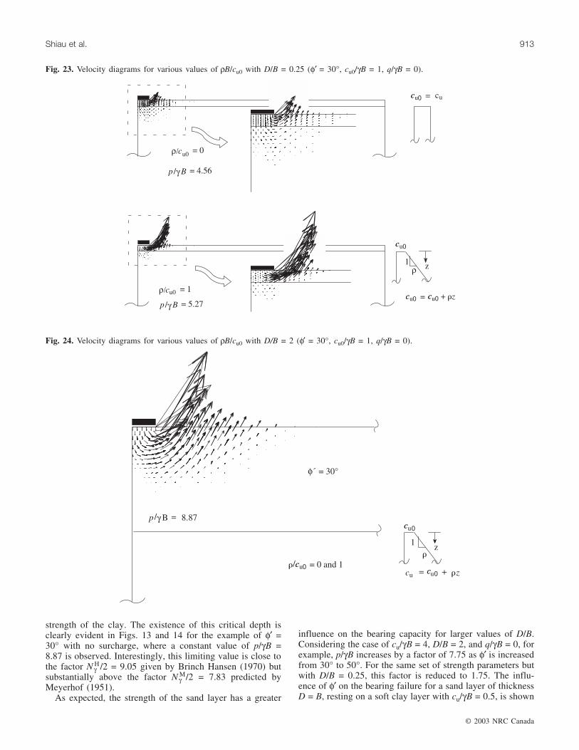
Fig. 21. Effect of increasing strength with depth for clay forD/B = 0.25.

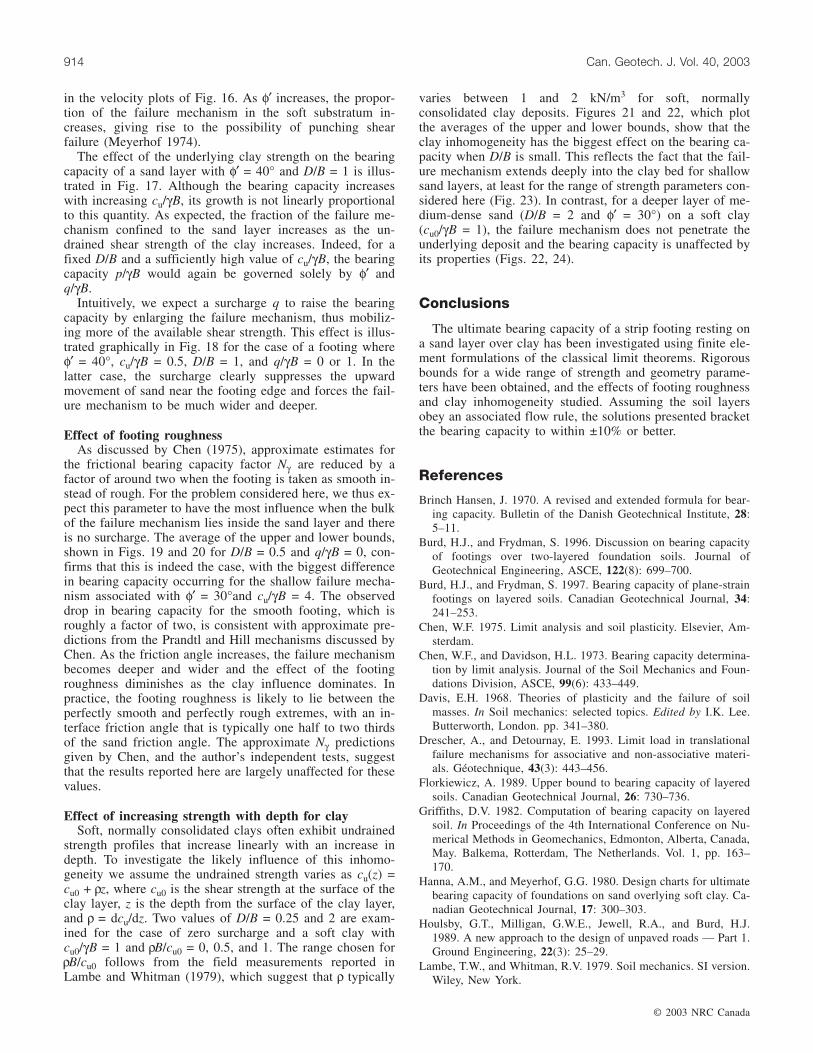
Fig. 22. Effect of increasing strength with depth for clay forD/B = 2.



strength of the clay. The existence of this critical depth isclearly evident in Figs. 13 and 14 for the example of φ′ =30° with no surcharge, where a constant value of p/γB =8.87 is observed. Interestingly, this limiting value is close tothe factor Nγ

H/2 = 9.05 given by Brinch Hansen (1970) butsubstantially above the factor Nγ

M/2 = 7.83 predicted byMeyerhof (1951).

As expected, the strength of the sand layer has a greater

influence on the bearing capacity for larger values of D/B.Considering the case of cu/γB = 4, D/B = 2, and q/γB = 0, forexample, p/γB increases by a factor of 7.75 as φ′ is increasedfrom 30° to 50°. For the same set of strength parameters butwith D/B = 0.25, this factor is reduced to 1.75. The influ-ence of φ′ on the bearing failure for a sand layer of thicknessD = B, resting on a soft clay layer with cu/γB = 0.5, is shown

© 2003 NRC Canada

Shiau et al. 913

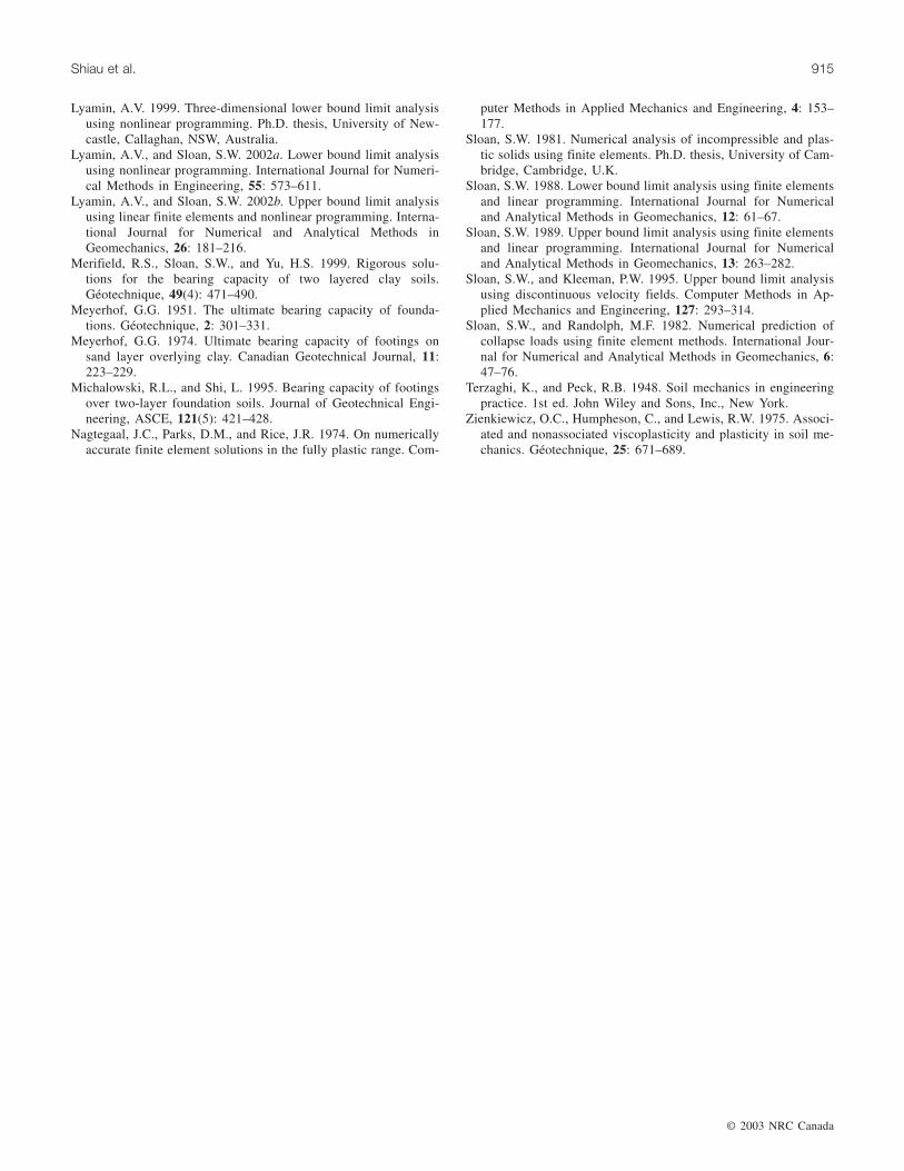
Fig. 23. Velocity diagrams for various values of ρB/cu0 with D/B = 0.25 (φ′ = 30°, cu0/γB = 1, q/γB = 0).

Fig. 24. Velocity diagrams for various values of ρB/cu0 with D/B = 2 (φ′ = 30°, cu0/γB = 1, q/γB = 0).



in the velocity plots of Fig. 16. As φ′ increases, the propor-tion of the failure mechanism in the soft substratum in-creases, giving rise to the possibility of punching shearfailure (Meyerhof 1974).

The effect of the underlying clay strength on the bearingcapacity of a sand layer with φ′ = 40° and D/B = 1 is illus-trated in Fig. 17. Although the bearing capacity increaseswith increasing cu/γB, its growth is not linearly proportionalto this quantity. As expected, the fraction of the failure me-chanism confined to the sand layer increases as the un-drained shear strength of the clay increases. Indeed, for afixed D/B and a sufficiently high value of cu/γB, the bearingcapacity p/γB would again be governed solely by φ′ andq/γB.

Intuitively, we expect a surcharge q to raise the bearingcapacity by enlarging the failure mechanism, thus mobiliz-ing more of the available shear strength. This effect is illus-trated graphically in Fig. 18 for the case of a footing whereφ′ = 40°, cu/γB = 0.5, D/B = 1, and q/γB = 0 or 1. In thelatter case, the surcharge clearly suppresses the upwardmovement of sand near the footing edge and forces the fail-ure mechanism to be much wider and deeper.

Effect of footing roughnessAs discussed by Chen (1975), approximate estimates for

the frictional bearing capacity factor Nγ are reduced by afactor of around two when the footing is taken as smooth in-stead of rough. For the problem considered here, we thus ex-pect this parameter to have the most influence when the bulkof the failure mechanism lies inside the sand layer and thereis no surcharge. The average of the upper and lower bounds,shown in Figs. 19 and 20 for D/B = 0.5 and q/γB = 0, con-firms that this is indeed the case, with the biggest differencein bearing capacity occurring for the shallow failure mecha-nism associated with φ′ = 30°and cu/γB = 4. The observeddrop in bearing capacity for the smooth footing, which isroughly a factor of two, is consistent with approximate pre-dictions from the Prandtl and Hill mechanisms discussed byChen. As the friction angle increases, the failure mechanismbecomes deeper and wider and the effect of the footingroughness diminishes as the clay influence dominates. Inpractice, the footing roughness is likely to lie between theperfectly smooth and perfectly rough extremes, with an in-terface friction angle that is typically one half to two thirdsof the sand friction angle. The approximate Nγ predictionsgiven by Chen, and the author’s independent tests, suggestthat the results reported here are largely unaffected for thesevalues.

Effect of increasing strength with depth for claySoft, normally consolidated clays often exhibit undrained

strength profiles that increase linearly with an increase indepth. To investigate the likely influence of this inhomo-geneity we assume the undrained strength varies as cu(z) =cu0 + ρz, where cu0 is the shear strength at the surface of theclay layer, z is the depth from the surface of the clay layer,and ρ = dcu/dz. Two values of D/B = 0.25 and 2 are exam-ined for the case of zero surcharge and a soft clay withcu0/γB = 1 and ρB/cu0 = 0, 0.5, and 1. The range chosen forρB/cu0 follows from the field measurements reported inLambe and Whitman (1979), which suggest that ρ typically

varies between 1 and 2 kN/m3 for soft, normallyconsolidated clay deposits. Figures 21 and 22, which plotthe averages of the upper and lower bounds, show that theclay inhomogeneity has the biggest effect on the bearing ca-pacity when D/B is small. This reflects the fact that the fail-ure mechanism extends deeply into the clay bed for shallowsand layers, at least for the range of strength parameters con-sidered here (Fig. 23). In contrast, for a deeper layer of me-dium-dense sand (D/B = 2 and φ′ = 30°) on a soft clay(cu0/γB = 1), the failure mechanism does not penetrate theunderlying deposit and the bearing capacity is unaffected byits properties (Figs. 22, 24).

Conclusions

The ultimate bearing capacity of a strip footing resting ona sand layer over clay has been investigated using finite ele-ment formulations of the classical limit theorems. Rigorousbounds for a wide range of strength and geometry parame-ters have been obtained, and the effects of footing roughnessand clay inhomogeneity studied. Assuming the soil layersobey an associated flow rule, the solutions presented bracketthe bearing capacity to within ±10% or better.

References

Brinch Hansen, J. 1970. A revised and extended formula for bear-ing capacity. Bulletin of the Danish Geotechnical Institute, 28:5–11.

Burd, H.J., and Frydman, S. 1996. Discussion on bearing capacityof footings over two-layered foundation soils. Journal ofGeotechnical Engineering, ASCE, 122(8): 699–700.

Burd, H.J., and Frydman, S. 1997. Bearing capacity of plane-strainfootings on layered soils. Canadian Geotechnical Journal, 34:241–253.

Chen, W.F. 1975. Limit analysis and soil plasticity. Elsevier, Am-sterdam.

Chen, W.F., and Davidson, H.L. 1973. Bearing capacity determina-tion by limit analysis. Journal of the Soil Mechanics and Foun-dations Division, ASCE, 99(6): 433–449.

Davis, E.H. 1968. Theories of plasticity and the failure of soilmasses. In Soil mechanics: selected topics. Edited by I.K. Lee.Butterworth, London. pp. 341–380.

Drescher, A., and Detournay, E. 1993. Limit load in translationalfailure mechanisms for associative and non-associative materi-als. Géotechnique, 43(3): 443–456.

Florkiewicz, A. 1989. Upper bound to bearing capacity of layeredsoils. Canadian Geotechnical Journal, 26: 730–736.

Griffiths, D.V. 1982. Computation of bearing capacity on layeredsoil. In Proceedings of the 4th International Conference on Nu-merical Methods in Geomechanics, Edmonton, Alberta, Canada,May. Balkema, Rotterdam, The Netherlands. Vol. 1, pp. 163–170.

Hanna, A.M., and Meyerhof, G.G. 1980. Design charts for ultimatebearing capacity of foundations on sand overlying soft clay. Ca-nadian Geotechnical Journal, 17: 300–303.

Houlsby, G.T., Milligan, G.W.E., Jewell, R.A., and Burd, H.J.1989. A new approach to the design of unpaved roads — Part 1.Ground Engineering, 22(3): 25–29.

Lambe, T.W., and Whitman, R.V. 1979. Soil mechanics. SI version.Wiley, New York.

© 2003 NRC Canada




© 2003 NRC Canada

Shiau et al. 915

Lyamin, A.V. 1999. Three-dimensional lower bound limit analysisusing nonlinear programming. Ph.D. thesis, University of New-castle, Callaghan, NSW, Australia.

Lyamin, A.V., and Sloan, S.W. 2002a. Lower bound limit analysisusing nonlinear programming. International Journal for Numeri-cal Methods in Engineering, 55: 573–611.

Lyamin, A.V., and Sloan, S.W. 2002b. Upper bound limit analysisusing linear finite elements and nonlinear programming. Interna-tional Journal for Numerical and Analytical Methods inGeomechanics, 26: 181–216.

Merifield, R.S., Sloan, S.W., and Yu, H.S. 1999. Rigorous solu-tions for the bearing capacity of two layered clay soils.Géotechnique, 49(4): 471–490.

Meyerhof, G.G. 1951. The ultimate bearing capacity of founda-tions. Géotechnique, 2: 301–331.

Meyerhof, G.G. 1974. Ultimate bearing capacity of footings onsand layer overlying clay. Canadian Geotechnical Journal, 11:223–229.

Michalowski, R.L., and Shi, L. 1995. Bearing capacity of footingsover two-layer foundation soils. Journal of Geotechnical Engi-neering, ASCE, 121(5): 421–428.

Nagtegaal, J.C., Parks, D.M., and Rice, J.R. 1974. On numericallyaccurate finite element solutions in the fully plastic range. Com-

puter Methods in Applied Mechanics and Engineering, 4: 153–177.

Sloan, S.W. 1981. Numerical analysis of incompressible and plas-tic solids using finite elements. Ph.D. thesis, University of Cam-bridge, Cambridge, U.K.

Sloan, S.W. 1988. Lower bound limit analysis using finite elementsand linear programming. International Journal for Numericaland Analytical Methods in Geomechanics, 12: 61–67.

Sloan, S.W. 1989. Upper bound limit analysis using finite elementsand linear programming. International Journal for Numericaland Analytical Methods in Geomechanics, 13: 263–282.

Sloan, S.W., and Kleeman, P.W. 1995. Upper bound limit analysisusing discontinuous velocity fields. Computer Methods in Ap-plied Mechanics and Engineering, 127: 293–314.

Sloan, S.W., and Randolph, M.F. 1982. Numerical prediction ofcollapse loads using finite element methods. International Jour-nal for Numerical and Analytical Methods in Geomechanics, 6:47–76.

Terzaghi, K., and Peck, R.B. 1948. Soil mechanics in engineeringpractice. 1st ed. John Wiley and Sons, Inc., New York.

Zienkiewicz, O.C., Humpheson, C., and Lewis, R.W. 1975. Associ-ated and nonassociated viscoplasticity and plasticity in soil me-chanics. Géotechnique, 25: 671–689.



Documents

Bearing capacity of a sand layer on clay by finite element ... · Bearing capacity of a sand layer on clay by finite element limit analysis J.S. Shiau, A.V. Lyamin, and S.W. Sloan