BEARING CAPACITY OF A STRIP FOOTING

ON A LAYERED COHESIONLESS SOIL

Brad Carter

(3129513)

Senior Report

CE 5943

November 2005

Abstract

Two critical aspects of footing design are: bearing capacity and settlement of the

underlying soil. Currently, analytical methods that have not been fully verified are used

to determine these aspects of design. The purpose of this study is to verify the theories

for the specific case of a strip footing over a layered cohesionless soil with the upper

layer being dense and the lower layer being loose.

Seven tests were conducted using the geotechnical centrifuge at the University of New

Brunswick to monitor the settlements of a model strip footing under central load. From

these tests, the ultimate bearing capacity was determined. The observed capacities were

compared with the theoretical values predicted in past studies. It was found that the

results of this study generally agree with the previous studies, but with minor differences.

It was predicted that when the layer of dense soil less than 1.5 times the width of the

footing, punching would be the governing mode of failure and when the upper dense

layer was thicker then 1.5 B bearing capacity or the dense layer would govern. In the

present study, punching was found to govern for a dense layer of soil with a depth equal

to the base of the footing and not 1.5 times the base of the footing.

It was found that Schmertmann’s method generally gave conservative values for the

amount of predicted settlement in cases where the dense layer of soil was less than two

times the width of the footing. More tests will be needed to confirm this difference.

ii

Acknowledgements

I would like to acknowledge Dr. A. J. Valsangkar for his advice and guidance during the

completion of this study.

I would further like to thank Mr. Dan Wheaton for his advices on assembly of the model,

as well as for fabricating the needed components, and operating the centrifuge.

iii

Table of Contents Abstract ............................................................................................................................... ii

Acknowledgements............................................................................................................ iii

List of Figures .................................................................................................................... vi

List of Tables ..................................................................................................................... vi

List of Symbols ................................................................................................................. vii

1 Introduction................................................................................................................. 1

1.1 Problem Statement .............................................................................................. 1

1.2 Objectives ........................................................................................................... 1

1.3 Background......................................................................................................... 1

2 Literature Review........................................................................................................ 3

2.1 Ultimate Bearing Capacity.................................................................................. 3

2.2 Settlement ........................................................................................................... 6

2.3 UNB’s Geotechnical Centrifuge ......................................................................... 6

2.3.1 Theory and Scale Relations ........................................................................ 7

2.3.2 Modeling Considerations............................................................................ 8

3 Methodology............................................................................................................. 10

3.1 Phases of Study................................................................................................. 10

3.2 Centrifuge Testing ............................................................................................ 10

3.2.1 Calibration ................................................................................................ 10

3.2.2 Model Assembly ........................................................................................ 12

3.2.3 Final Test Preparations ............................................................................ 14

3.2.4 Test ............................................................................................................ 15

3.3 Data Analysis .................................................................................................... 16

4 Results....................................................................................................................... 17

4.1 Test Results....................................................................................................... 17

4.2 Theoretical Results............................................................................................ 18

4.2.1 Ultimate Bearing Capacity ....................................................................... 18

4.2.2 Settlement .................................................................................................. 19

5 Discussions ............................................................................................................... 20

5.1 Experimental vs. Theoretical ............................................................................ 20

iv

5.1.1 Ultimate Bearing Capacity ....................................................................... 20

5.1.2 Settlement .................................................................................................. 21

5.2 Problems Encountered ...................................................................................... 22

6 Conclusions............................................................................................................... 23

7 Recommendations..................................................................................................... 24

References......................................................................................................................... 25

Appendix A – Data Collection Run Graphs ..................................................................... 26

Appendix B – Bearing Capacity Calculations .................................................................. 33

v

List of Figures

Figure 2-1 - Reference Diagram (Meyerhof, 1974)............................................................ 4

Figure 2-2 – Values of Ks (Meyerhof, 1978) ..................................................................... 5

Figure 2-3 - Assumed distribution of strain influence factor with depth (Das, 1990)........ 6

Figure 3-1 - Filling the Strongbox with Sand ................................................................... 12

Figure 3-2 - Levelling Sand with Vacuum ....................................................................... 12

Figure 3-3 - The Jig Placed in the Strongbox ................................................................... 13

Figure 3-4 - Placing the Model Footing using the Jig ...................................................... 13

Figure 3-5 - Footing with Load Cell and LSC's................................................................ 14

Figure 3-6 - Apparatus ...................................................................................................... 14

Figure 4-1 - Measured Load vs. Displacement................................................................. 18

Figure 5-1 - Experimental Results and Theoretical Results ............................................. 21

List of Tables

Table 2.1 - Scale Relations (Stewart, 2000) ....................................................................... 8

Table 3.1 - Channels used for electronics......................................................................... 15

Table 4.1 - Theoretical vs. measured ultimate bearing capacity and φ ............................ 19

Table 4.2 - Settlements for 50 kPa pressure ..................................................................... 19

vi

List of Symbols

B The width of the footing

c1 Correction factor for footing depth

c2 Correction factor for creep

D Depth of footing

Ez Young’s Modulus

g Acceleration due to gravity

H The depth of the soil to the loose layer

hm Height of model

Iz Strain influence factor

Kp Coefficient of passive earth pressure

Ks Coefficient of punching shear

N Scale factor

N γ, Nq Bearing capacity factors

Pp Total passive earth pressure

qlower Bearing capacity of lower layer

qn Net foundation pressure

qu Ultimate bearing capacity

Re Effective radius of rotation

Rt Radius at top of model

s Settlement

αm Acceleration of the model

αp Acceleration of the prototype

δ mobilized friction of truncated pyramid

γt Unit weight of upper soil layer

γ Unit weight of soil

φ Soil internal angle of friction

vii

ω Angular rotation speed

Δz Thickness of sand layer

viii

1 Introduction

1.1 Problem Statement

This study examines the bearing capacity of a strip footing on a layered cohesionless soil

using physical modeling. The results of the experiment are compared with existing

theories.

1.2 Objectives

The study had the following objectives:

• Model a footing on a layered soil using a geotechnical centrifuge.

• Compare the results with the existing theories of the bearing capacity and settlement

of footings on layered soils.

1.3 Background

A footing is used to transmit the load from a structure to the soil on a larger area to

reduce the pressure. Different types of footings are used for different applications. The

footing type used in this study is a strip footing which is largely used to support a linear

load such as a load bearing wall or a retaining wall. A strip footing is rectangular in

shape but its length is much greater than its width. Analysing a strip footing is a simple

case as it can be analysed in two dimensions.

When a structure is built, the soil on which the footing is to be founded is generally

compacted to provide a firm base. Since the compaction extends only a finite depth into

the soil it can create a dense soil over loose soil condition. It is important to know in

these situations, how much load a soil can support so that the soil does not fail in bearing

capacity under the loads applied by the structure. There are theoretical formulas which

can be used to determine bearing capacity for such layered soils. These formulas have

been in use for many years and have not been thoroughly verified. The lack of testing is

due to the difficulty of the tests. One option of testing is to build a full size footing and

test it for determining bearing capacity. While this would provide good results, a test

such as this is both expensive and difficult to accomplish. A second option is to test 1-g

1

scale models. This is the most common method as it is much less costly and the scale

models are easy to handle. However, the results from testing in this manner may not be

fully accurate as some factors are lost in the scaling(Taylor, 1995). A third approach is to

use centrifuge modeling. A scaled model when accelerated higher than that of gravity

will behave as a larger model. This allows for ease of handling and more representative

results for prototype structures.

In order to study bearing capacity of a footing in the specific case of dense sand over

loose sand, the thickness of the upper layers in relation to the width of the footing was

varied.

2

2 Literature Review

2.1 Ultimate Bearing Capacity

If the ultimate bearing capacity of the dense sand layer is much greater than that of the

underlying loose deposit it can be approximated by considering the failure as an inverted

uplift problem. At the ultimate load a sand mass having an approximately truncated

pyramidal shape is pushed into the lower sand layer in such a way that the friction angle

φ and the bearing capacity of the lower layer are mobilized in the combined failure zones

(Meyerhof, 1974). The ultimate bearing capacity of the layered soil should be equal to

bearing capacity of the lower layer plus the punching resistance of the upper layer and the

contribution due to surcharge.

The forces on the failure surface of the sand can be taken as total passive earth pressures

inclined at an angle δ acting upwards on a vertical plane through the footings edge.

Therefore the ultimate bearing capacity according do Meyerhof (1974), qu, of a strip

footing can be taken as

DB tγ

δ++=

)sin(2Pq q p

loweru .............................................................. (1)

Where:

qlower = bearing capacity of the lower sand layer,

Pp = total passive earth pressure,

δ = mobilized friction on truncated pyramid,

B = footing width, and

γt = unit weight of upper sand

3

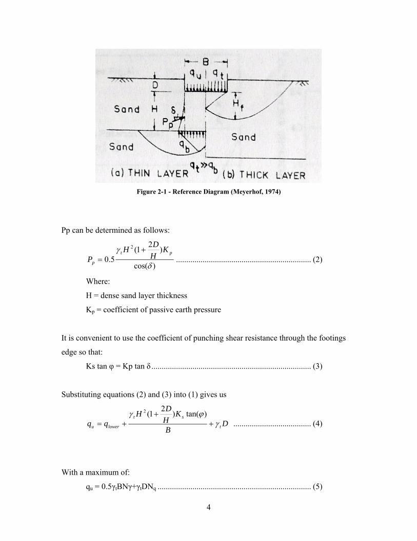
Figure 2-1 - Reference Diagram (Meyerhof, 1974)

Pp can be determined as follows:

)cos(

)21(5.0

2

δ

γ pt

p

KHDH

P+

= .................................................................. (2)

Where:

H = dense sand layer thickness

Kp = coefficient of passive earth pressure

It is convenient to use the coefficient of punching shear resistance through the footings

edge so that:

Ks tan φ = Kp tan δ .............................................................................. (3)

Substituting equations (2) and (3) into (1) gives us

DB

KHDH

qq t

st

loweru γϕγ

++

+=)tan()21(2

...................................... (4)

With a maximum of:

qu = 0.5γtBNγ+γtDNq ........................................................................... (5)

4

The maximum occurs when the H/B ratio is high enough such that the upper layer no

longer fails through punching and its bearing capacity governs the bearing capacity of the

layered soil system.

The factor Ks can be determined from the following figure provided by Meyerhof and

Hanna’s 1978 study on the Ultimate bearing capacity of foundations on layered soils

under inclined load.

Figure 2-2 – Values of Ks (Meyerhof, 1978)

5

2.2 Settlement

Schmertmann’s method is commonly used for estimating the amount of settlement due to

a load. It is based on a simplified version of vertical strain under a footing in the form of

a strain influence factor, Iz, as seen in Figure 2.3. The settlement is determined with the

equation: (Craig 1997)

∑ Δ=B

z

zn z

EIqccs

4

021 .............................................................................. (6)

Where, c1 = correction factor for footing depth

c2 = correction factor for creep

qn = net foundation pressure

B = width of footing

Iz = strain influence factor

Ez = Young’s Modulus

= thickness of the layer zΔ

Figure 2-3 - Assumed distribution of strain influence factor with depth (Das, 1990)

2.3 UNB’s Geotechnical Centrifuge

The centrifuge was commissioned in 1990 and is capable of inertial acceleration of up to

200gs at an effective radius of 1.6 meters. Each arm of the centrifuge can hold a load up

to 100 kg. The data acquisition is on arm supporting up to 16 channels and transmits to

6

the control room in real time through slip rings with one slip ring reserved for the

introduction of fluids. These data are then collected and stored by a computer program

called GEN2000.

2.3.1 Theory and Scale Relations

A centrifuge accelerates the model by rotating it at high revolutions per minute (rpm).

When the model is accelerated in this manner it experiences forces like earth’s gravity

but increased proportionally by a factor N. When the model is spun at high g’s, it

behaves like a prototype structure, N times its size. (Taylor, 1995) The inertial

acceleration of the model αm is denoted by:

αm= ω2Re .............................................................................................. (7)

Where ω = angular rotational speed

Re= the effective centrifuge radius

As the radius varies over the depth of a model, an effective radius needs to be determined

since the factors influenced by gravity will also vary over the depth of the model.

Re = Rt + Hm/3 ..................................................................................... (8)

Where Rt = Radius at the top of the model

Hm = the height or depth of model

Since N is the multiple of the model feels over the field of gravity it can be seen that

αm = Nαp............................................................................................... (9)

Where αp the acceleration the prototype experiences

The acceleration that the prototype experiences is due to gravity therefore it can be seen

therefore g can replace αp with g

αm = Ng ................................................................................................ (10)

Combining equations (7) and (10),

ω2Re= Ng.............................................................................................. (11)

7

Only forces which are normally affected by gravity are influenced by the centrifuge as

since it acts as an increased gravitational force on an object. The scaling laws are

presented in the following table. Table 2.1 - Scale Relations (Stewart, 2000)

Quantity Full Scale (Prototype) Centrifuge Model @Ng’s

Linear Dimension 1 1/N

Area 1 1/N2

Volume 1 1/N3

Velocity 1 1

Acceleration 1 N

Mass 1 1/N3

Force 1 1/N2

Stress 1 1

Strain 1 1

Density 1 1

2.3.2 Modeling Considerations

There are some factors that affect the results of the centrifuge tests that would not occur

in the real situations - such as, the model being confined in a box. The wall boundaries

exert sidewall friction on the soil. Sidewall friction is not major factor for this particular

experiment as all measurements are being taken from the surface and the model footing is

placed in the centre of the box a distance of 4.5B from the walls. Particle size must be

accounted for as well; it is logical to assume that the particle size increases by a factor of

the force of gravity like the model does, so fine sand could increase in size to represent

gravel (Taylor 1995). It is suggested that the effects of particle size can be avoided by

keeping the major model dimensions greater than 15 times that of the soil.

8

Another consideration is the fact that the factor N varies through the depth of the model.

In this experiment the distance from the top to the bottom of the model is 100 mm which

is relatively small. An effective radius is used which is located at the top third of the

model is used. The variation of N from the top of the model to the bottom of the model is

approximately 8%.

9

3 Methodology

Five tests were performed on a model of a footing at a rate of 30g’s. The depth of the

dense sand was varied with the loose sand to determine how this affected the results.

While a range near 30g’s was used for the testing this was not on purpose; instead, it is

due to the difficulty of running the centrifuge at an exact g-level. This should not affect

the results as it would only change the proportional value N which can be accounted for

in the calculations.

The factor H will be examined as a ratio to the width B. At 4 times the width of the

footing most of the stress from the load on the footing will have been dissipated. For that

reason, 4 times the width of the footing will be the lower bound for the thickness of the

dense sand with tests being run at 0B, 1B, 2B, 3B, and 4B.

3.1 Phases of Study

There were 3 phases of study:

1) Design and assembly of the model and apparatus: in this phase all the materials

needed to perform the tests were gathered and any modifications to existing

equipment were performed.

2) Testing the model on the centrifuge: during this phase the model was run on the

centrifuge 5 times at varying depths of dense and loose sand.

3) The final phase was analysis of the data: During this phase all of the collected

data from phase 2 were analysed.

3.2 Centrifuge Testing

3.2.1 Calibration

The load cell was calibrated first. The load cell allows for the measurement applied load

to the footing to be measured. At loads of varying and known intensity voltages were

10

measured in the load cell, a linear regression of these data points allowed for the

establishment of the calibration curve.

The LSC’s were calibrated with the GEN2000 computer program using a two point

calibration method. The distance LSC was extended was measured and noted in the

GEN2000 program. Finally the LSC was fully compressed and this was also noted in the

GEN2000 program. The procedure was then repeated for the other LSC.

3.2.2 Model Footing

The model footing was a steel bar with the base dimensions of 194 mm x 25 mm. When

accelerated to a rate of 30g’s it will simulate a footing of 5.82 m x 0.75 m. This will

approximate a strip footing.

3.2.3 Sand Placement

The strongbox used to hold the sand had internal dimensions of 197 mm x 254 mm x 194

mm deep. Since only 100 mm of room in the box was needed for the sand a 76 mm thick

wooden block was placed at the bottom. This allowed the soil sample to be closer to the

top of the box and the measuring devices.

Sand was air pluviated into the Strongbox from a hopper which was suspended over the

strongbox bolted on the centrifuge arm. The total depth of sand was 100 mm, which was

composed of a layer of dense sand over layer of loose sand. The loose sand was placed

in the strongbox first by maintaining a drop height of 0.5 cm. The dense sand was placed

in the box using a drop height of 40 cm. The dense layer was placed in approximately 1

cm lifts rather than the constant height at which the loose soil was maintained. Figure 3.1

shows the placement of the dense layer.

11

Figure 3-1 - Filling the Strongbox with Sand

Once the Box had been filled to slightly above 100 mm, the surface of the sand was

vacuumed level with a shop-vac and a leveling guide. This ensured that the top of the

sand was level. Vacuuming is demonstrated in Figure 3.2.

Figure 3-2 - Levelling Sand with Vacuum

3.2.2 Model Assembly

Once the sand was placed, the final assembly of the model and the measuring instruments

was performed. First the model footing was placed with a light wooden jig that was

constructed to allow for correct model placement. The model was carefully placed on the

12

sand so as not to compact the sand underneath. This process is shown in Figures 3.3 and

3.4

Figure 3-3 - The Jig Placed in the Strongbox

Figure 3-4 - Placing the Model Footing using the

Jig

Once the footing was placed the jig was removed and the pneumatic ram was bolted on

the strongbox. A small ball-bearing was placed on the center of the footing to act as a

contact point between the piston and the footing. Once the ball bearing was placed on the

footing the piston was carefully extended until it was almost touching the ball-bearing.

The LSC’s were then ready to be placed into their machined locations on the pneumatic

ram. The LSC’s were placed in such a manner that they are fully compressed. As the

footing is pushed into the soil they extend and correspond to the footing settlement.

Finally the lines which carry the nitrogen to operate the pneumatic ram are connected to

the hydraulic slip ring of the centrifuge. A photograph of the footing, LSC’s, and the

load cell is shown in Figure 3.5 and a sketch of the final apparatus can be seen in Figure

3.6.

13

Figure 3-5 - Footing with Load Cell and LSC's

Figure 3-6 - Apparatus

3.2.3 Final Test Preparations

The centrifuge needs to be properly balanced as the model is mounted on one arm of the

centrifuge. The weight of sand is approximated by the sand having an approximated

density of 1500kg/m3 and a known volume. Finally the strongbox, wood block and

apparatus all have known masses allowing an equal mass to be placed on the other arm of

the centrifuge.

14

The final procedure is for all the measuring devices to be connected into the electronic

panel on the centrifuge. The devices were connected into the following channels:

Table 3.1 - Channels used for electronics

Instrument Channel

LSC 2 2

LSC 1 3

Load Cell 1

Accelerometer 0

Finally the centrifuge area was cleared of all debris and the room vacated prior to starting

the centrifuge.

3.2.4 Test

From the control room the data logger is started followed by the starting of the centrifuge.

The data is logged during the acceleration of the centrifuge. Though these data were not

used in the actual calculation, they give an indication of how the model is performing

under self weight. This was especially important with the test when entirely loose sand

was tested as the model nearly failed under its own self weight.

The centrifuge is accelerated to as close to 30 g’s as possible without going under 30 g’s.

Once the required speed has been reached, the load is then applied the footing with a tank

of nitrogen located in the control room. Due to the valve on the nitrogen tank it was

difficult to slowly increase the pressure, so rather then smooth increases the pressure was

increased in steps. As load was being increased, the deflection of the footing was

monitored up to a displacement of 13 mm.

Finally the footing was unloaded and the centrifuge stopped. During the slowing down

of the centrifuge data logging was not carried out.

15

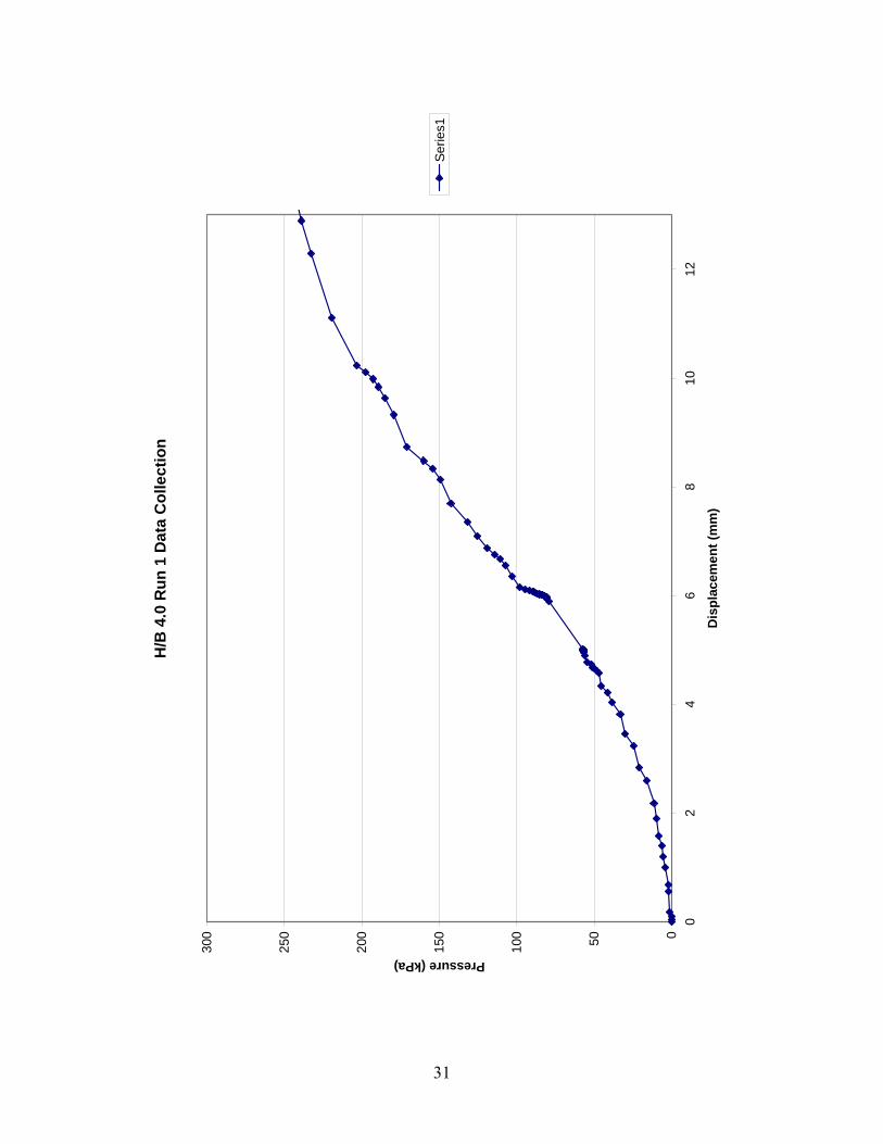
3.3 Data Analysis

The results of the data collection are then imported into excel as CVS data and plotted as

load vs. deflection. The point of failure is determined and the pressure is determined from

that, using the footings area

Aloadq f = ............................................................................................ (12)

Where:

load = load at failure

A = area of footing

Once qf is determined φ is needed. To determine φ the relationship between Nγ and Nq

(Craig 1997) is used.

qf = 0.5γtB Nγ + γtD Nq ........................................................................ (13)

Nq=exp(πtan(φ))tan2(45 + φ/2) .......................................................... (14)

Nγ = (Nq-1)tan(φ) ................................................................................ (15)

Equations (13), (14), and (15) are then combined to give us an equation which can be

used to solve for φ.

qf =0.5γtB (exp(πtan(φ))tan2(45 + φ/2)-1)tan(φ) + γtD exp(πtan(φ))tan2(45 + φ/2) ............................................................................................................. (16)

All quantities are known in the equation except φ.

All of the measured data can now be compared with the theoretical equations to

determine φ.

Once φ has been determined the theoretical bearing capacity will be calculated using the

equation qu = qlower+γtH2(1+2D/H)Kstan(φ)/B + γtD (which was shown in the literature

review portion of this report).

16

4 Results

Seven centrifuge tests were completed. The maximum bounds from which φ and qlower

was derived from were completed twice, with the other 3 tests were for the H/B ratios of

0.5, 1, 2. The results are presented in Figure 4.1, and individual data runs are presented

in Appendix A.

4.1 Test Results

The ultimate bearing capacity was determined at 12 mm deflection or a settlement of

approximately 50% of the base width. A structure would not tolerate a deflection of

nearly 50% of the base width and as such this value was used to define qf.

The results which are presented in Figure 4.1 show a general trend of increasing bearing

capacity as the thickness of the upper dense layer increases. This result is as expected; as

the upper layer becomes thicker more force will be required to punch through the upper

dense layer. Once the upper layer reaches sufficient thickness, punching is no longer the

governing mode of failure. This is demonstrated in that H/B of 2 and 4 having similar

results.

The reading from the load cell was multiplied by g or 9.81m/s2 to determine the force

applied to the footing. This force is then divided by the footing area to obtain a pressure.

17

Load vs Displacement

0

25

50

75

100

125

150

175

200

225

250

275

300

325

350

375

0 1 2 3 4 5 6 7 8 9 10 11 12 13

Displacement (mm)

Pres

sure

(kPa

) 0 H/B0.5 H/B1 H/B2 H/B4 H/B4 H/B (run 2)

Figure 4-1 - Measured Load vs. Displacement

4.2 Theoretical Results

The experimental results were compared with the theoretical results based on the

equations outlined in the literature review.

4.2.1 Ultimate Bearing Capacity

Using equation (16), φ for dense layer was determined to be 43.6o and φ for the loose

layer was determined to be 28.3 o, though φ for the loose layer is not needed in any

calculations. The measured bearing capacity for H/B ratio of 0 is used for the value of

qlower. Using φdense , qlower, and γt in equation (4), theoretical values can be calculated for

the different H/B ratios. See Appendix B for calculations. The results are summarized in

the following table:

18

Table 4.1 - Theoretical vs. measured ultimate bearing capacity and φ

H/B Ratio Theoretical

Ultimate Bearing

Capacity (kPa)

Measured Ultimate

Bearing Capacity

(kPa)

Percent Difference

(%)

0.5 75.9 99.9 31.6

1 155.2 157.3 1.4

2 420.8 229.7 -45.4

φdense = 43.6o φloose = 28.3 o

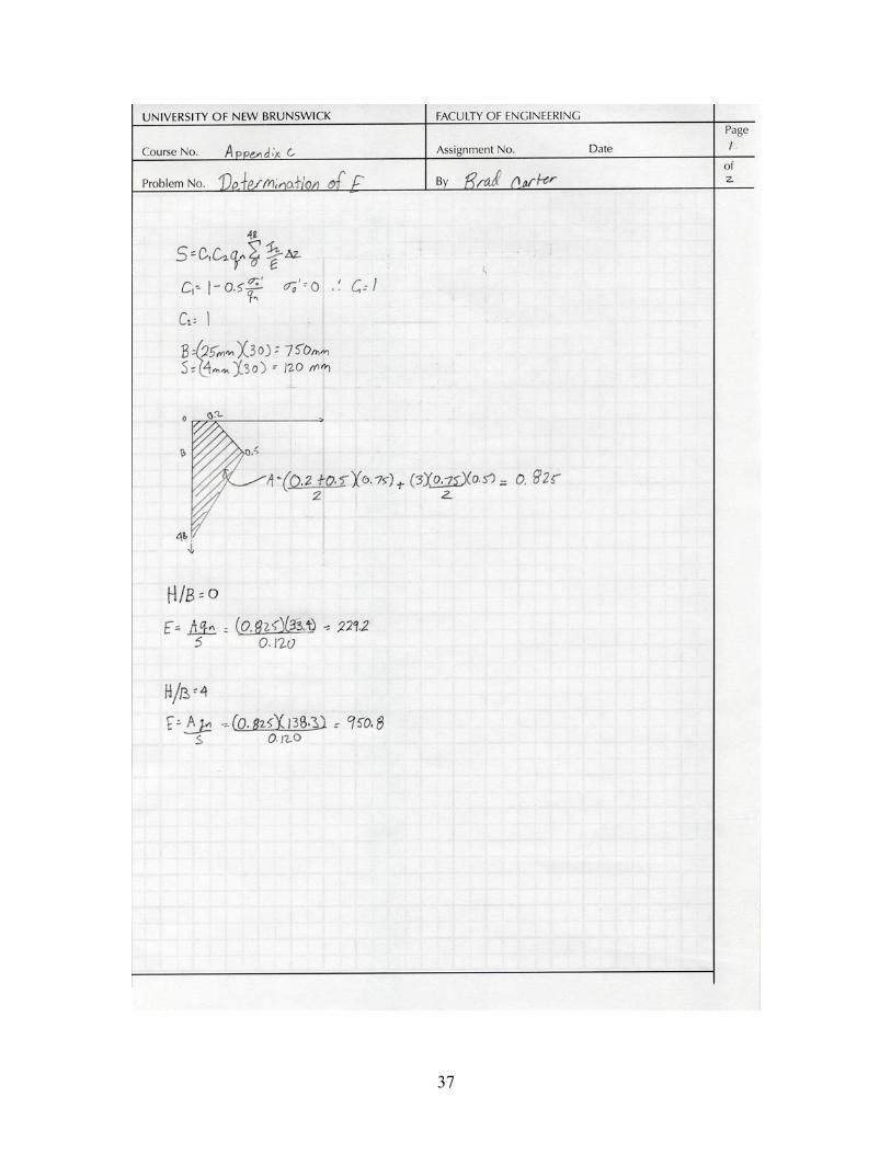
4.2.2 Settlement

The theoretical settlement values were determined using Schmertmann’s method as

outlined in the literature study. The value for Young’s Modulus, E, for dense and loose

soils was determined by using the measured pressures at 4 mm settlement and solving for

E. These E values were then used to calculate the settlements at a pressure of 50 kPa for

the H/B ratios of 0.5, 1, and 2. Calculations are shown in appendix C.

Table 4.2 - Settlements for 50 kPa pressure

H/B Ratio Theoretical

Settlement (mm)

Measured Settlement

(mm)

Percent

Difference (%)

0.5 170 141 20.6

1.0 143 111 28.8

2.0 88 90 -2.2

19

5 Discussions

The results are discussed further in this section.

5.1 Experimental vs. Theoretical

5.1.1 Ultimate Bearing Capacity

The experimental results of this study were compared with the theoretical values based

on Meyerhof’s findings for the expected bearing capacity of the footing on a layered soil.

As seen in the following figure (Figure 5.1) the theoretical estimates for H/B greater than

1 start to overestimate the actual bearing capacity of the soil. It can also be seen that

increasing the thickness of the upper sand layer increases the bearing capacity until an

H/B of 2 is reached. However the equation which assumes a punching failure for the

upper sand layer overestimates the capacity of the upper soil. As the upper layer

becomes thicker it is less likely to fail in punching and more likely to be a standard

bearing capacity failure. This is likely what is happening between the H/B ratio of 1 and

2.

20

Calculated Results and Measured results

0

100

200

300

400

500

600

0.5 1 1.5 2

H/B

qf(k

Pa)

Calculated ResultsMeasured Results

Figure 5-1 - Experimental Results and Theoretical Results

5.1.2 Settlement

Schmertmann’s method provided generally good results. In all cases but H/B = 2, the

theoretical values were greater than the measured. The value predicted for settlement

with H/B = 2 is very close with approximately a 2% difference. This difference could

possibly be accounted for with experimental error. Since no tests were completed for

H/B ratios between 2 and 4, it is unknown if the values between 2 and 4 are accurately

predicted.

As can be seen in Figure 5.2, the predicted settlements for the theoretical and the

measured values are changing at different rates. This is due to the predicted values

following the 2 linear lines in the strain influence diagram, whereas the measured values

21

follow a non-linear shape. Though there is a difference in the curves they both have the

same general shape, making Schmertmann’s method a reasonable prediction.

Settlement vs Sand Thickness

0

20

40

60

80

100

120

140

160

180

0.5 1 2

H/B ratio

Settl

emen

t (m

m)

Theoretical Measured

Figure 5.2 - Settlement vs Sand Thickness

5.2 Problems Encountered

There were few problems encountered in this study. The problems encountered centred

on not being able to apply a load in fine enough increments. This created “jumps” in the

data. The solution which was used in this case was to do some of the tests twice to try

and pick up missing data points.

22

6 Conclusions

This study has shown that as the upper dense layer of a soil increases in thickness the

ultimate bearing capacity generally increases up until an H/B ratio of 1. The following

conclusions can be derived about a footing on dense sand over loose sand

• Meyerhof’s findings for sand over clay can be applied to the dense sand over

loose sand with the difference that it only applies until an H/B ratio of 1 is

reached.

• At an H/B ratio of about 1 the failure is less to do with a punching failure from

the dense sand but increasingly more of a standard bearing failure. At an H/B

ratio of about 2 the dense layer of sand is no longer experiencing punching

failure.

• Schmertmann’s method overestimates the settlement which the footing

experiences for H/B ratios less than 2, but otherwise it provides a reasonable

estimate.

23

7 Recommendations

From this study 3 recommendations can be made

1) Redo the testing with an apparatus which can apply a load in finer increments so a

smoother curve can be derived

2) More testing is needed for H/B ratio of 1 and some testing of for an H/B ratio of

1.5 to get more results around the critical area which the punching failure starts to

convert to a bearing failure

3) Test at least one run at a H/B ratio of 3 to determine if the theoretical settlement is

still underestimated.

24

References

Craig, R.F. 1997. Soil Mechanics, 6th Ed. Spon Press, London New York

Das, B.M, 1990. Principles of Foundation Engineering. PWS-Kent, Boston.

Meyerhof G.G. 1974. Ultimate Bearing Capacity of Footings on Sand Layer Overlaying

Clay. Canadian Geotechnical Journal, 11(2) pp 223-229.

Myerhof G.G., Hanna A.M, 1978. Ultimate bearing capacity of footings on layered soils

under an inclined load. Canadian Geotechnical Journal, 15, pp 565-572

Stewart, Marcie 2000. Smooth Strip Footing on a Finite Layer of Sand Over a Rigid

Boundary. University of New Brunswick, Fredericton

Taylor, RN 1995. Geotechnical Centrifuge Technology. Blackie Academic and

Professional, Bishopbriggs, Glasgow.

25

Appendix A – Data Collection Run Graphs

26

H/B

0 D

ata

Col

lect

ion

051015202530354045

02

46

810

12

Dis

plac

emen

t (m

m)

Pressure (kPa)

27

H/B

0.5

Dat

a C

olle

ctio

n

020406080100

120

02

46

810

12

Dis

plac

emen

t (m

m)

Pressure (kPa)

28

H/B

1.0

Dat

a C

olle

ctio

n

020406080100

120

02

46

810

12

Dis

plac

emen

t (m

m)

Pressure (kPa)

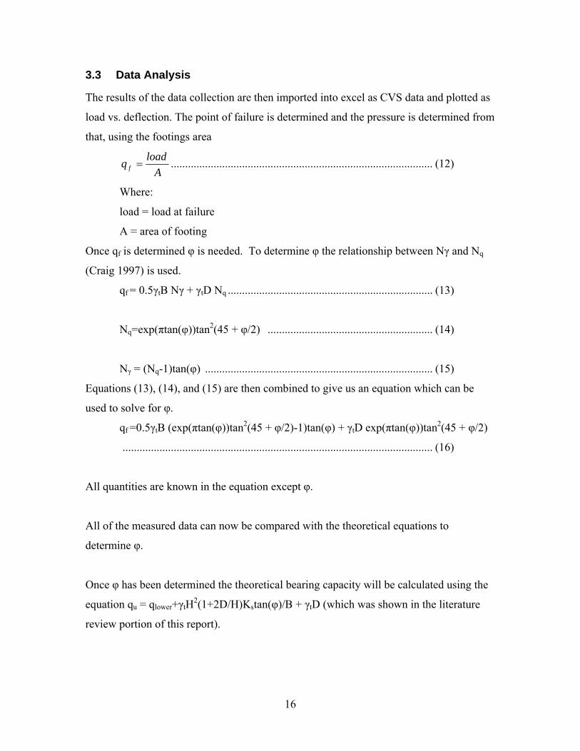
29

H/B

2.0

Dat

a C

olle

ctio

n

020406080100

120

140

160

180

02

46

810

12

Dis

plac

emen

t (m

m)

Pressure (kPa)

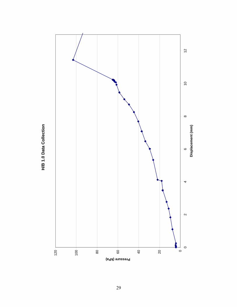
30

H/B

4.0

Run

1 D

ata

Col

lect

ion

050100

150

200

250

300

02

46

810

12

Dis

plac

emen

t (m

m)

Pressure (kPa)

Serie

s1

31

H/B

4.0

Run

2 D

ata

Col

lect

ion

050100

150

200

250

300

02

46

810

12

Dis

plac

emen

t (m

m)

Pressure (kPa)

Serie

s1

32

Appendix B – Bearing Capacity Calculations

33

34

35

Appendix C - Settlement Calculations

36

37

38