Embed Size (px)
Citation preview

Bearing Capacity
of Shallow
Foundations
INTRODUCTION
Bearing capacity is the power of foundation soil to hold the forces from the
superstructure without undergoing shear failure or excessive settlement.
Foundation soil is that portion of ground which is subjected to additional
stresses when foundation and superstructure are constructed on the
ground. The following are a few important terminologies related to bearing
capacity of soil.
Super Structure
Foundation
Foundation Soil
Ground Level
Ultimate Bearing Capacity (qf) : It is the maximum pressure that a
foundation soil can withstand without undergoing shear failure.
Net ultimate Bearing Capacity (qn) : It is the maximum extra pressure (in
addition to initial overburden pressure) that a foundation soil can withstand
without undergoing shear failure.
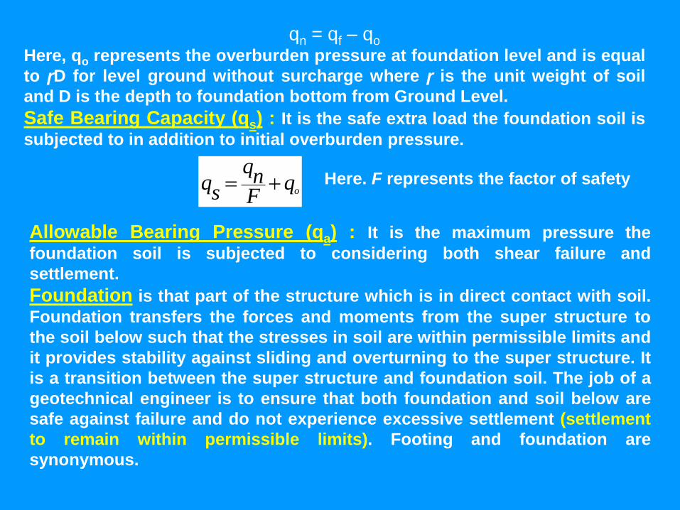
qn = qf – qo
Here, qo represents the overburden pressure at foundation level and is equal
to ɼD for level ground without surcharge where ɼ is the unit weight of soil
and D is the depth to foundation bottom from Ground Level.
Safe Bearing Capacity (qs) : It is the safe extra load the foundation soil is
subjected to in addition to initial overburden pressure.
oqFnq
sq
Allowable Bearing Pressure (qa) : It is the maximum pressure the
foundation soil is subjected to considering both shear failure and
settlement.
Foundation is that part of the structure which is in direct contact with soil.
Foundation transfers the forces and moments from the super structure to
the soil below such that the stresses in soil are within permissible limits and
it provides stability against sliding and overturning to the super structure. It
is a transition between the super structure and foundation soil. The job of a
geotechnical engineer is to ensure that both foundation and soil below are
safe against failure and do not experience excessive settlement (settlement
to remain within permissible limits). Footing and foundation are
synonymous.
Here. F represents the factor of safety
MODES OF SHEAR FAILUREDepending on the stiffness of foundation soil and depth of foundation, the
following are the modes of shear failure experienced by the foundation soil.
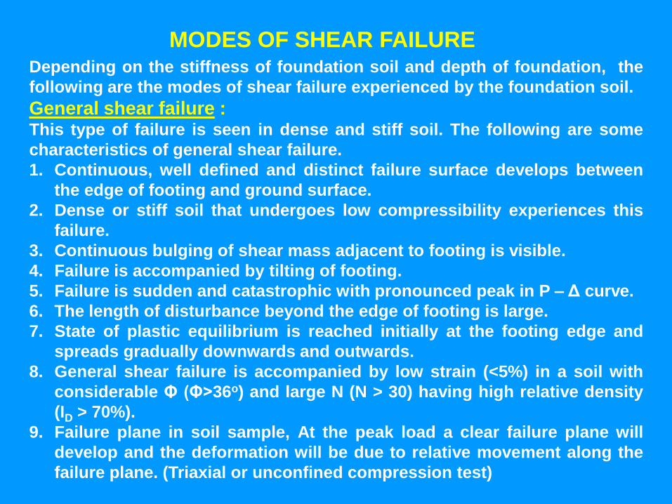
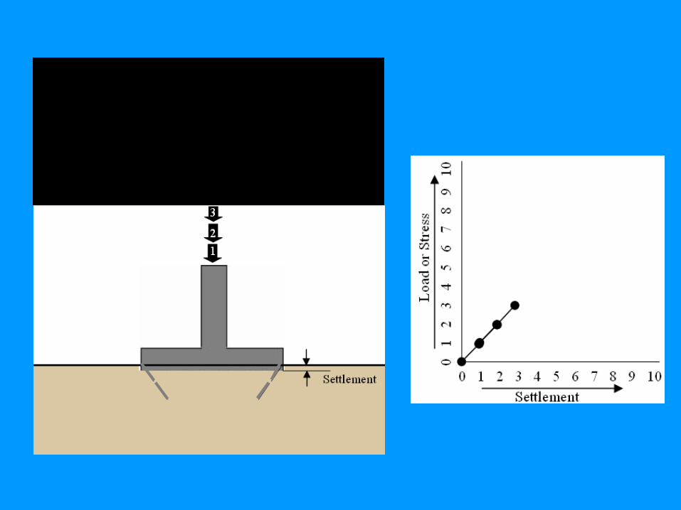
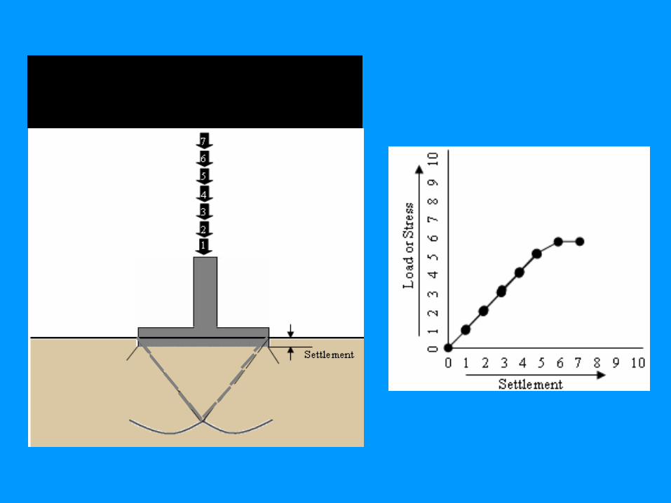
General shear failure :This type of failure is seen in dense and stiff soil. The following are some
characteristics of general shear failure.
1. Continuous, well defined and distinct failure surface develops between
the edge of footing and ground surface.
2. Dense or stiff soil that undergoes low compressibility experiences this
failure.
3. Continuous bulging of shear mass adjacent to footing is visible.
4. Failure is accompanied by tilting of footing.
5. Failure is sudden and catastrophic with pronounced peak in P – Δ curve.
6. The length of disturbance beyond the edge of footing is large.
7. State of plastic equilibrium is reached initially at the footing edge and
spreads gradually downwards and outwards.
8. General shear failure is accompanied by low strain (<5%) in a soil with
considerable Φ (Φ>36o) and large N (N > 30) having high relative density
(ID > 70%).
9. Failure plane in soil sample, At the peak load a clear failure plane will
develop and the deformation will be due to relative movement along the
failure plane. (Triaxial or unconfined compression test)
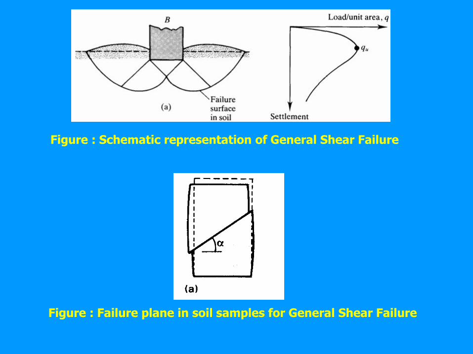
Figure : Schematic representation of General Shear Failure
Figure : Failure plane in soil samples for General Shear Failure
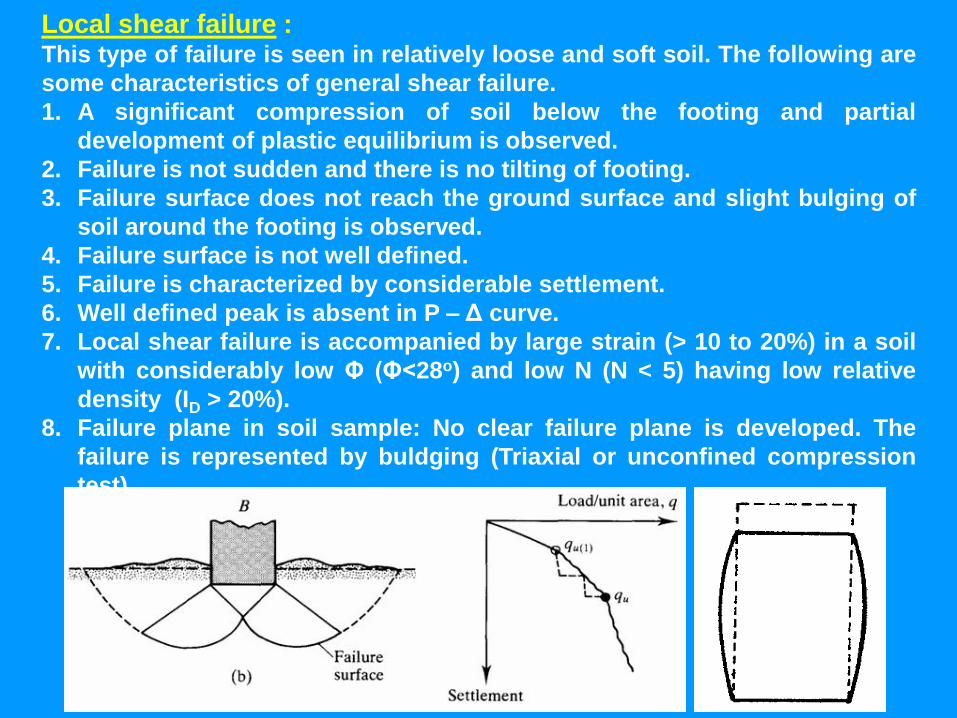
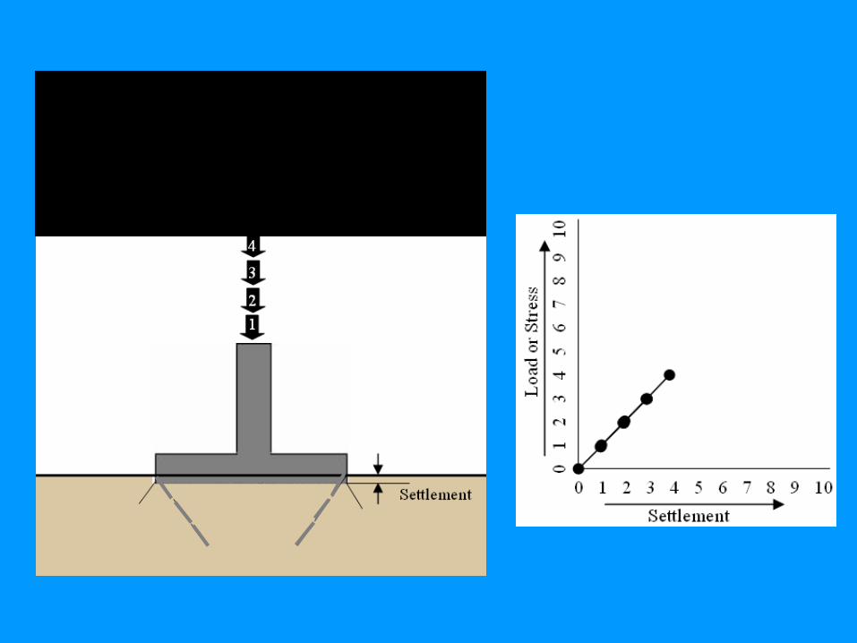
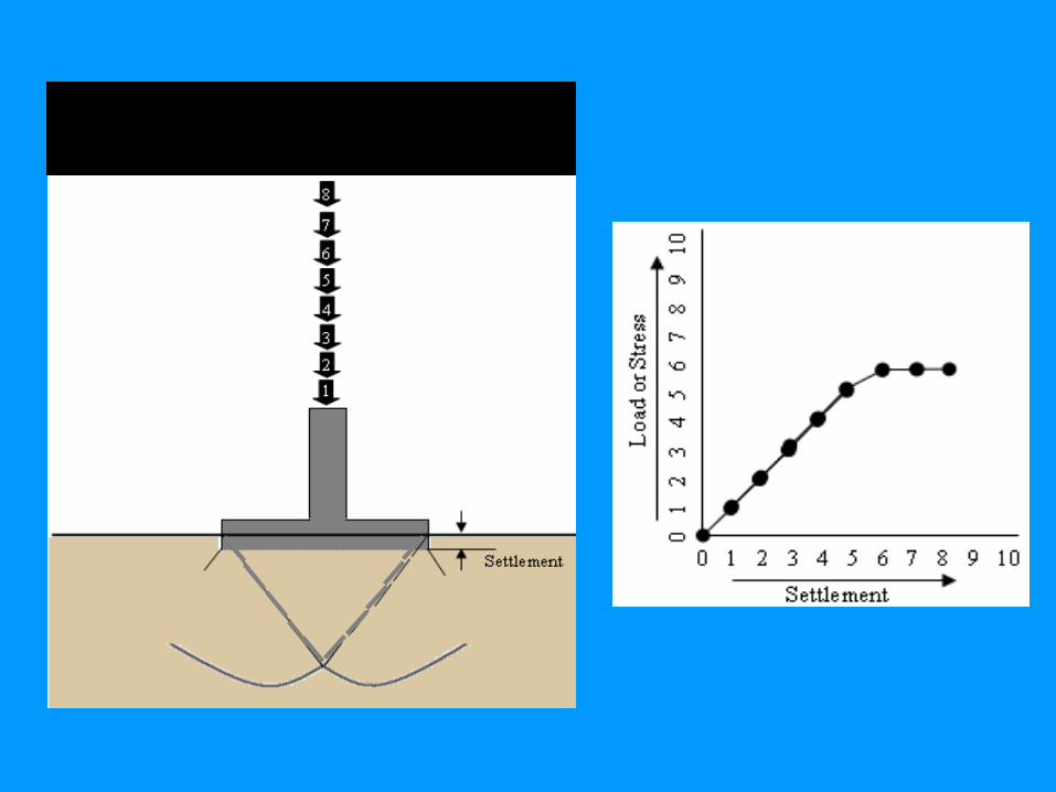
Local shear failure :This type of failure is seen in relatively loose and soft soil. The following are
some characteristics of general shear failure.
1. A significant compression of soil below the footing and partial
development of plastic equilibrium is observed.
2. Failure is not sudden and there is no tilting of footing.
3. Failure surface does not reach the ground surface and slight bulging of
soil around the footing is observed.
4. Failure surface is not well defined.
5. Failure is characterized by considerable settlement.
6. Well defined peak is absent in P – Δ curve.
7. Local shear failure is accompanied by large strain (> 10 to 20%) in a soil
with considerably low Φ (Φ<28o) and low N (N < 5) having low relative
density (ID > 20%).
8. Failure plane in soil sample: No clear failure plane is developed. The
failure is represented by buldging (Triaxial or unconfined compression
test)
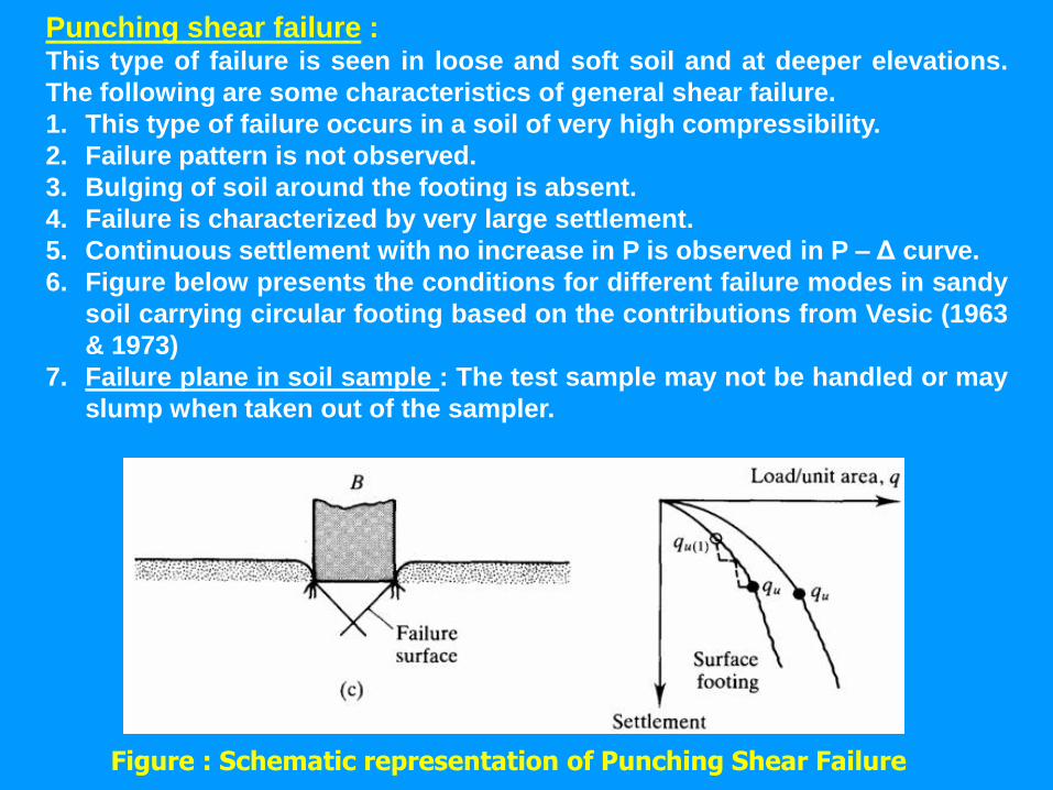
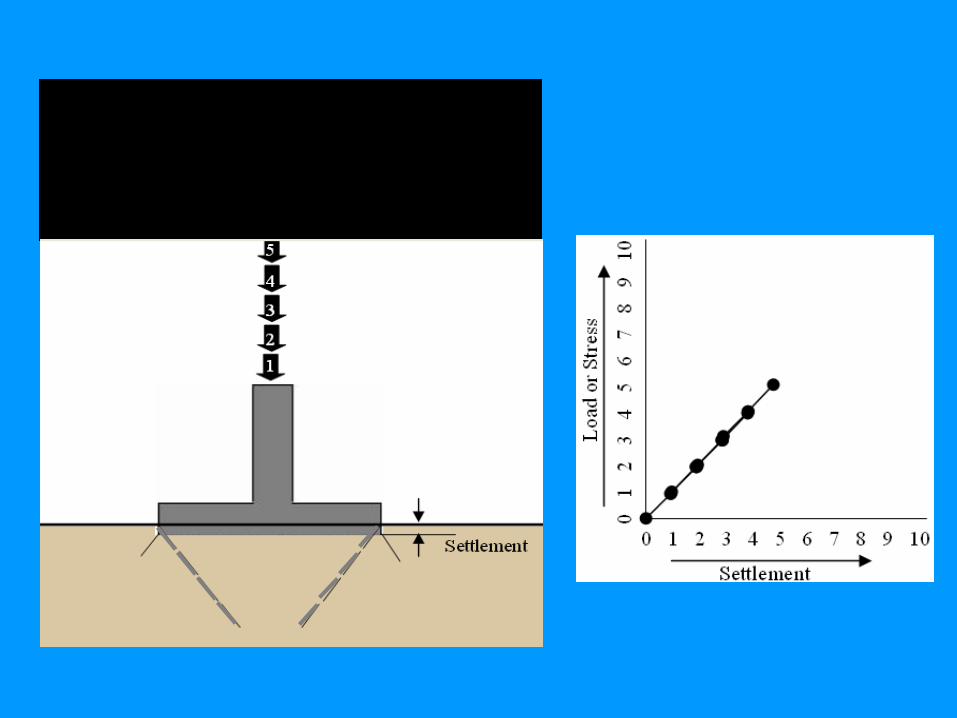
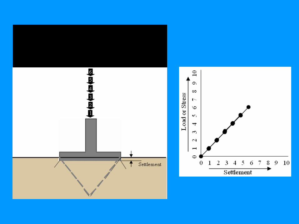
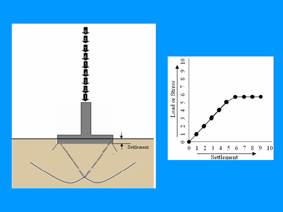
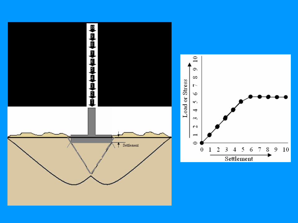
Punching shear failure :This type of failure is seen in loose and soft soil and at deeper elevations.
The following are some characteristics of general shear failure.
1. This type of failure occurs in a soil of very high compressibility.
2. Failure pattern is not observed.
3. Bulging of soil around the footing is absent.
4. Failure is characterized by very large settlement.
5. Continuous settlement with no increase in P is observed in P – Δ curve.
6. Figure below presents the conditions for different failure modes in sandy
soil carrying circular footing based on the contributions from Vesic (1963
& 1973)
7. Failure plane in soil sample : The test sample may not be handled or may
slump when taken out of the sampler.
Figure : Schematic representation of Punching Shear Failure
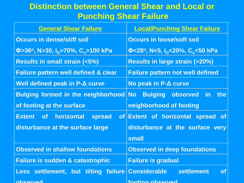
Distinction between General Shear and Local or
Punching Shear Failure
General Shear Failure Local/Punching Shear Failure
Occurs in dense/stiff soil
Φ>36o, N>30, ID>70%, Cu>100 kPa
Occurs in loose/soft soil
Φ<28o, N<5, ID<20%, Cu<50 kPa
Results in small strain (<5%) Results in large strain (>20%)
Failure pattern well defined & clear Failure pattern not well defined
Well defined peak in P-Δ curve No peak in P-Δ curve
Bulging formed in the neighborhood
of footing at the surface
No Bulging observed in the
neighborhood of footing
Extent of horizontal spread of
disturbance at the surface large
Extent of horizontal spread of
disturbance at the surface very
small
Observed in shallow foundations Observed in deep foundations
Failure is sudden & catastrophic Failure is gradual
Less settlement, but tilting failure
observed
Considerable settlement of
footing observed
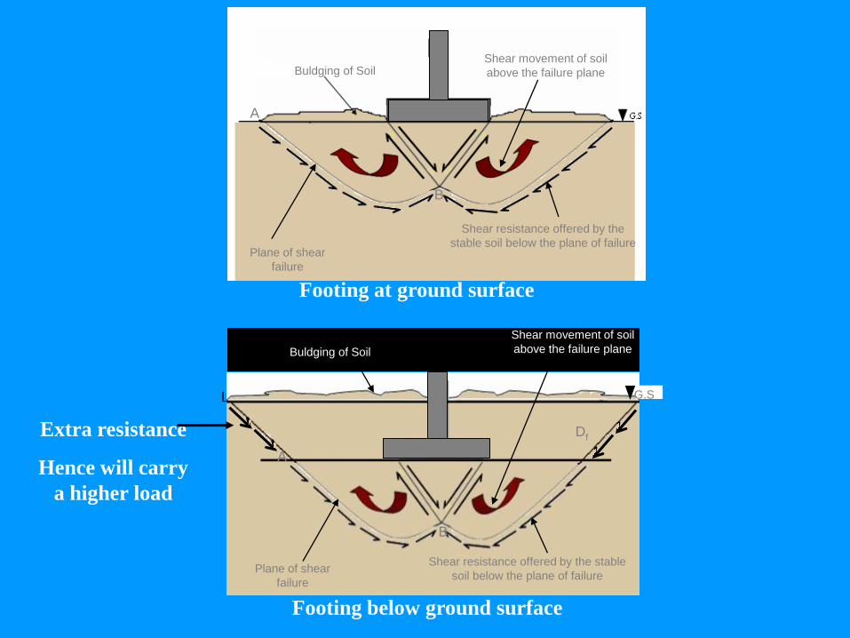
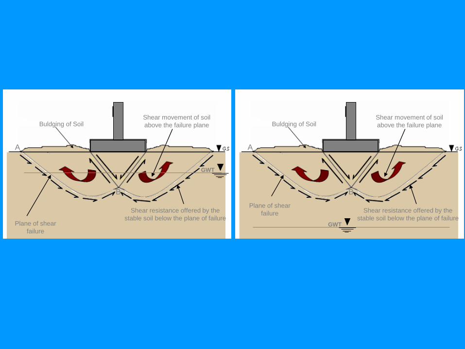
Plane of shear
failure
Shear resistance offered by the
stable soil below the plane of failure
Buldging of SoilShear movement of soil
above the failure plane
A
B
Plane of shear
failure
Shear resistance offered by the stable
soil below the plane of failure
A
B
G.S
Df
L
Shear movement of soil
above the failure plane Buldging of Soil
Footing at ground surface
Footing below ground surface
Extra resistance
Hence will carry
a higher load
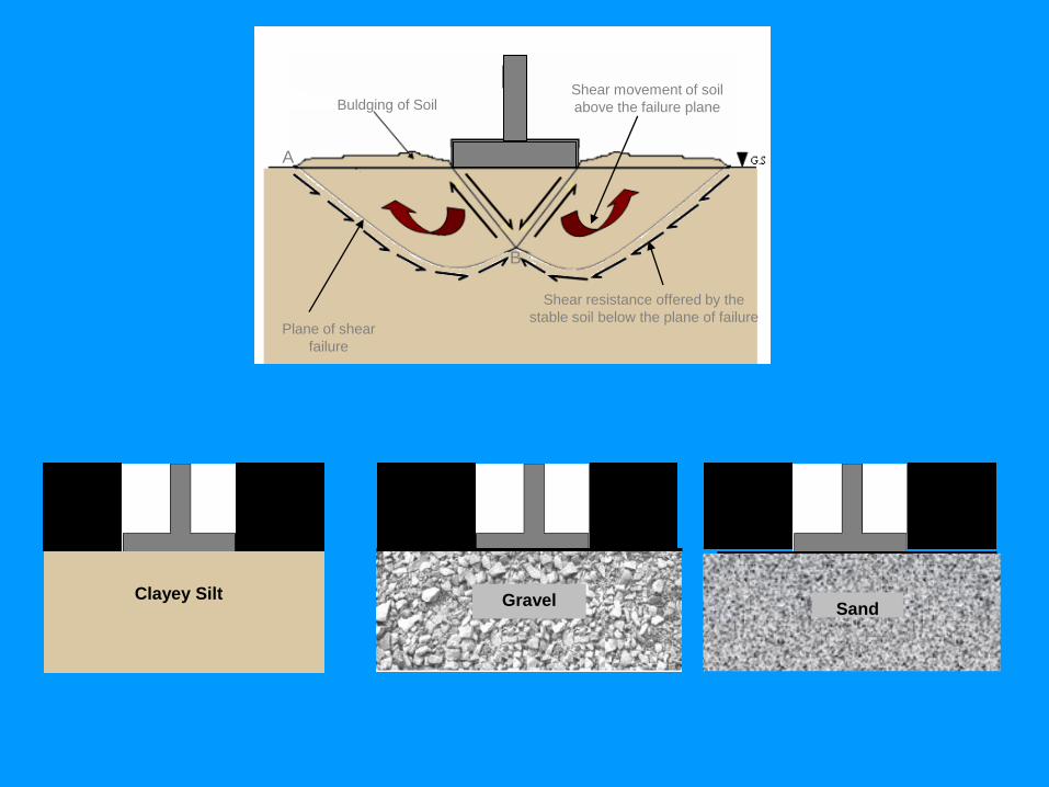
Clayey Silt GravelSand
Plane of shear
failure
Shear resistance offered by the
stable soil below the plane of failure
Buldging of SoilShear movement of soil
above the failure plane
A
B
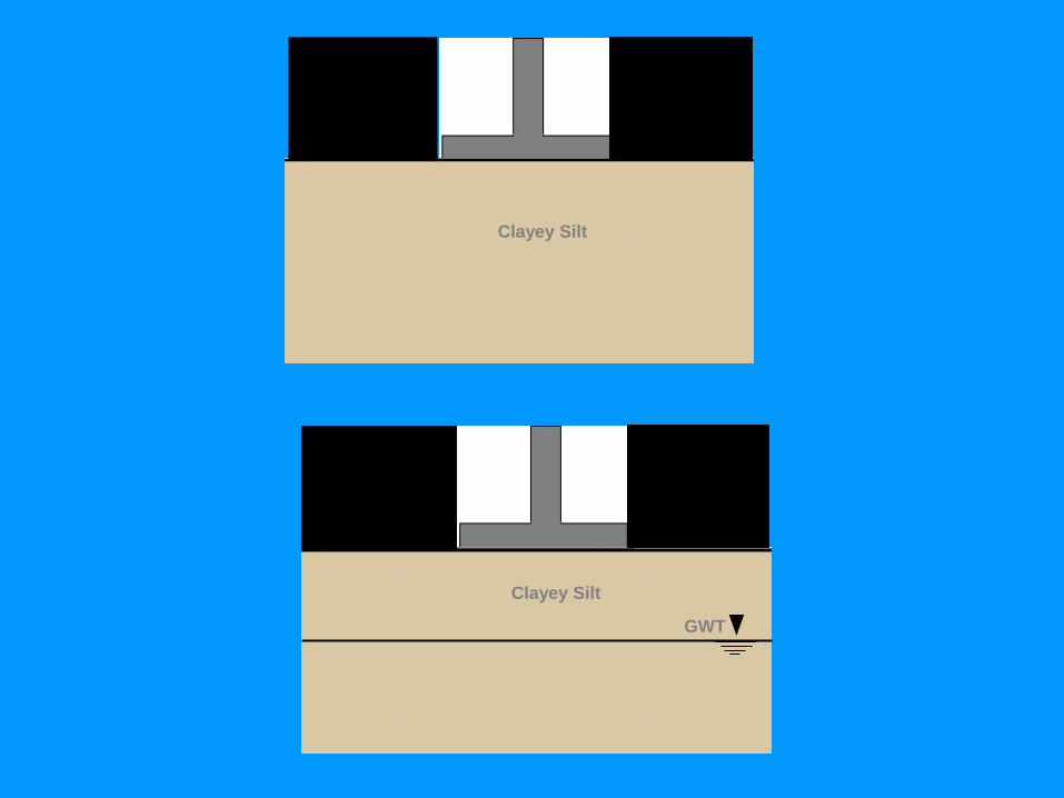
Clayey Silt
Clayey Silt
GWT
Plane of shear
failure
Shear resistance offered by the
stable soil below the plane of failure
Buldging of SoilShear movement of soil
above the failure plane
A
B
Plane of shear
failure Shear resistance offered by the
stable soil below the plane of failure
Buldging of SoilShear movement of soil
above the failure plane
A
B
GWT
GWT
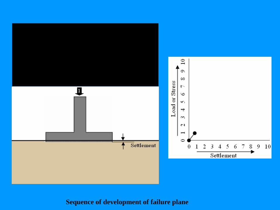
Sequence of development of failure plane
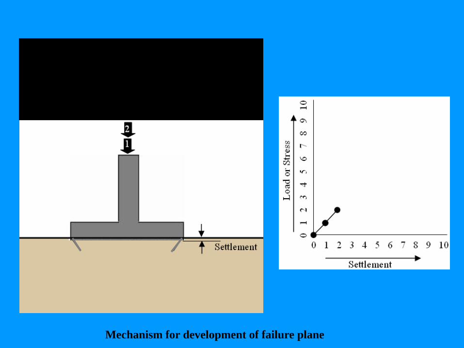
Mechanism for development of failure plane
RELATIONSHIP BETWEEN MODE OF FAILURE
AND RELATIVE DENSITY OF SAND
Based on experimental results, Vesic (1973) has proposed a
relationship for the mode of bearing capacity failure of foundations
resting on sands. This is shown in the following Figure, which uses the
following notations:
Dr = relative density of sand
Df = depth of foundation measured from the ground surface
Where
B = width of foundation
L = length of foundation
LB
BL*B
2
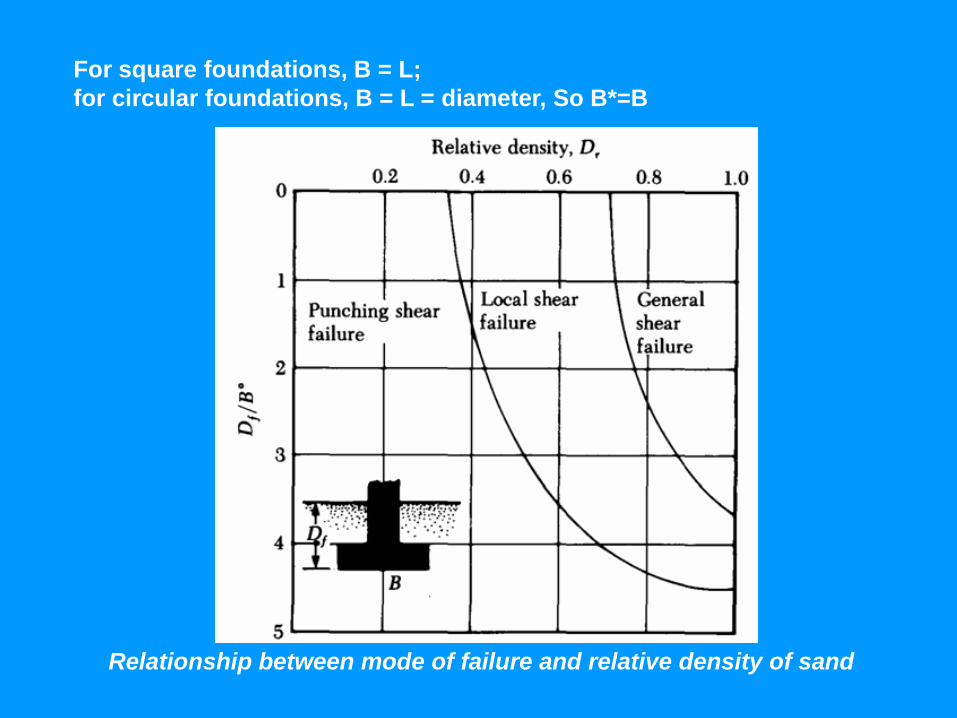
For square foundations, B = L;
for circular foundations, B = L = diameter, So B*=B
Relationship between mode of failure and relative density of sand
For foundations located at a shallow depth (that is, small Df/B*)
the ultimate load may be reached at a foundation settlement of
4—10% of B. This is true for general shear failure;
However, in the case of local or punching shear failure, the
ultimate load may be reached at settlements of 15—25% of the
width of foundation (B).
FACTOR AFFECTING BEARING CAPACITY OF SOIL
1. Soil Properties
a. Type of soil
b. Moisture content of soil
c. Density of soil
d. History of deposit
i. Recent fill
ii. Natural deposit
e. Layered soil
i. Strong soil layer overlying soft layer
ii. Soft soil layer overlying strong layer
2. Site Conditions
a. Sloping ground
b. Lateral confinement
c. Unstable ground condition
d. Mining activities
e. Frost penetration
i. Natural
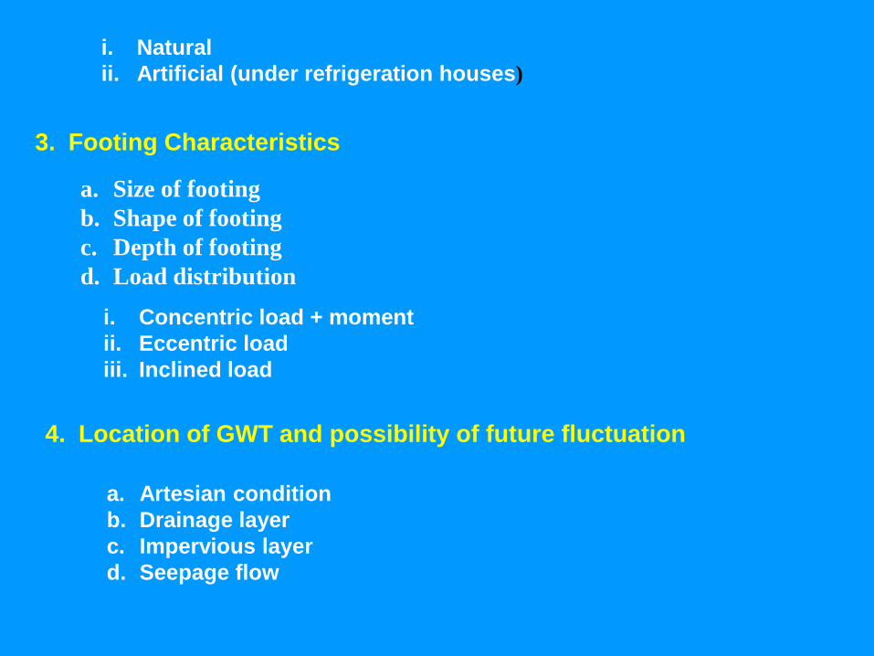
ii. Artificial (under refrigeration houses)
3. Footing Characteristics
a. Size of footing
b. Shape of footing
c. Depth of footing
d. Load distribution
i. Concentric load + moment
ii. Eccentric load
iii. Inclined load
4. Location of GWT and possibility of future fluctuation
a. Artesian condition
b. Drainage layer
c. Impervious layer
d. Seepage flow
5. Local conditions (time of investigation)
a. Weather conditions
b. Seismic activity
c. Flooding activity
6. Site History
a. Site developed after removal of wood. As long as the roots are
alive, these will act as reinforcement and will result in an
increase in bearing capacity. But when the roots decompose,
cavities will be produced causing decrease in soil density and
allow deep penetration of water causing decrease in shear
strength.
b. Agricultural lands
c. Reclaimed site
d. Site developed after demolition of building
e. Old fill with domestic waste
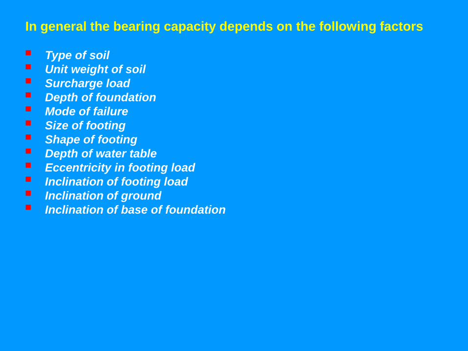
In general the bearing capacity depends on the following factors
Type of soil
Unit weight of soil
Surcharge load
Depth of foundation
Mode of failure
Size of footing
Shape of footing
Depth of water table
Eccentricity in footing load
Inclination of footing load
Inclination of ground
Inclination of base of foundation
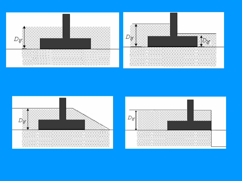
G.W.T
G.W.T
D3f
G.W.T
D3f
G.W.T
G.W.TG.W.T
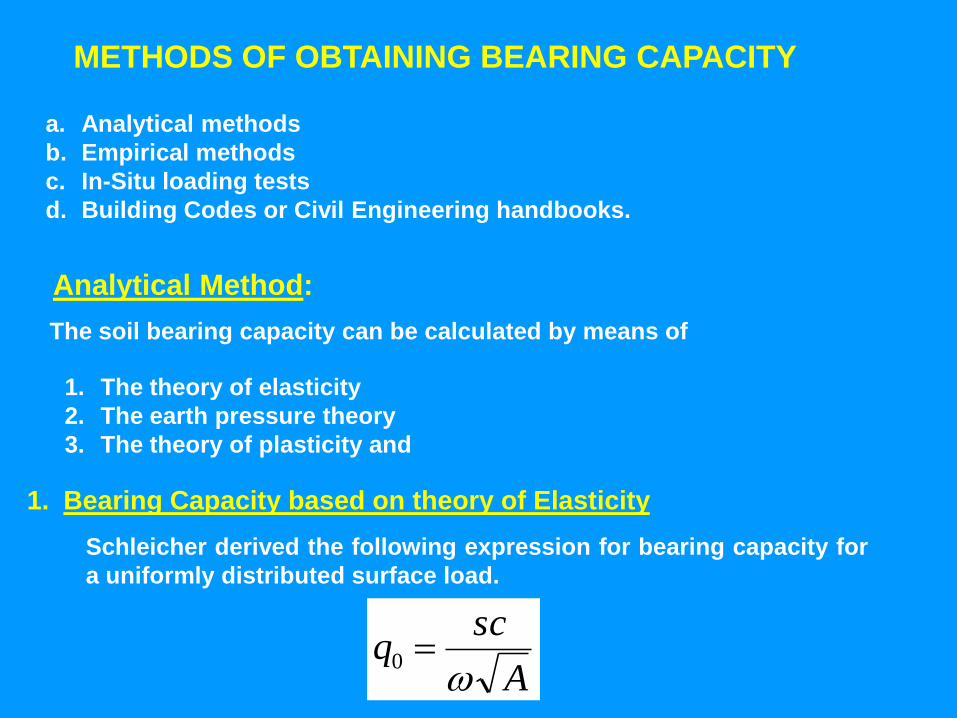
METHODS OF OBTAINING BEARING CAPACITY
a. Analytical methods
b. Empirical methods
c. In-Situ loading tests
d. Building Codes or Civil Engineering handbooks.
Analytical Method:
The soil bearing capacity can be calculated by means of
1. The theory of elasticity
2. The earth pressure theory
3. The theory of plasticity and
1. Bearing Capacity based on theory of Elasticity
Schleicher derived the following expression for bearing capacity for
a uniformly distributed surface load.
A
scq
0
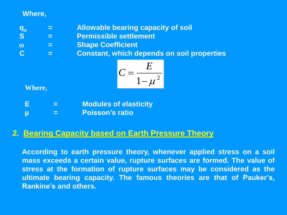
Where,
qo = Allowable bearing capacity of soil
S = Permissible settlement
= Shape Coefficient
C = Constant, which depends on soil properties
21
EC
Where,
E = Modules of elasticity
µ = Poisson‘s ratio
2. Bearing Capacity based on Earth Pressure Theory
According to earth pressure theory, whenever applied stress on a soil
mass exceeds a certain value, rupture surfaces are formed. The value of
stress at the formation of rupture surfaces may be considered as the
ultimate bearing capacity. The famous theories are that of Pauker‘s,
Rankine‘s and others.
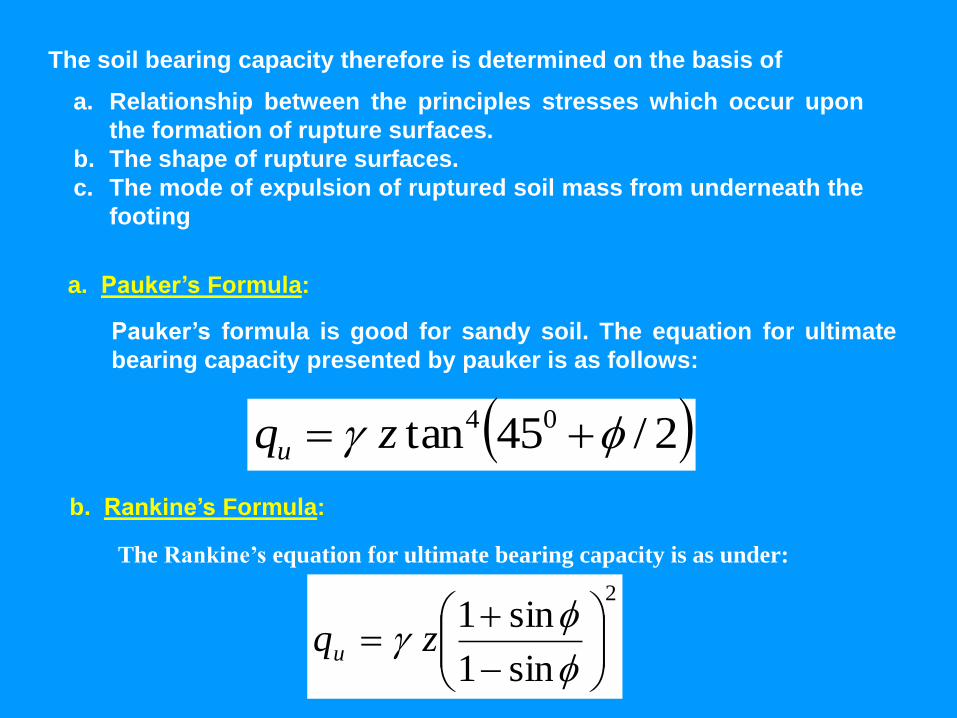
The soil bearing capacity therefore is determined on the basis of
a. Relationship between the principles stresses which occur upon
the formation of rupture surfaces.
b. The shape of rupture surfaces.
c. The mode of expulsion of ruptured soil mass from underneath the
footing
a. Pauker‘s Formula:
Pauker‘s formula is good for sandy soil. The equation for ultimate
bearing capacity presented by pauker is as follows:
2/45tan 04 zqu
b. Rankine‘s Formula:
The Rankine’s equation for ultimate bearing capacity is as under:
2
sin1
sin1
zqu
The above equations have many deficiencies and therefore are not used in
practice.
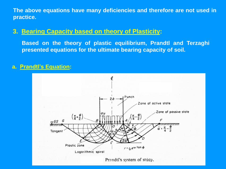
3. Bearing Capacity based on theory of Plasticity:
Based on the theory of plastic equilibrium, Prandtl and Terzaghi
presented equations for the ultimate bearing capacity of soil.
a. Prandtl‘s Equation:
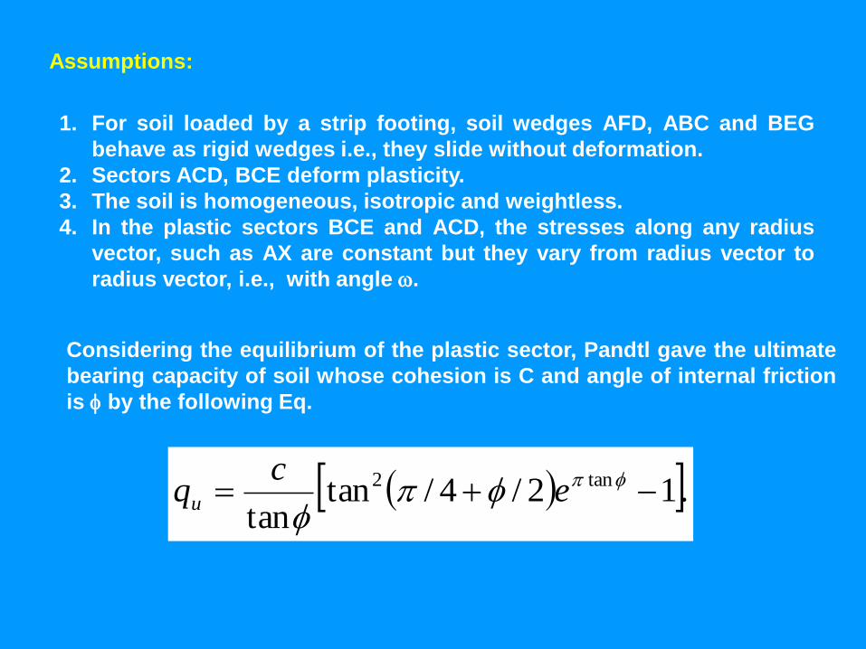
Assumptions:
1. For soil loaded by a strip footing, soil wedges AFD, ABC and BEG
behave as rigid wedges i.e., they slide without deformation.
2. Sectors ACD, BCE deform plasticity.
3. The soil is homogeneous, isotropic and weightless.
4. In the plastic sectors BCE and ACD, the stresses along any radius
vector, such as AX are constant but they vary from radius vector to
radius vector, i.e., with angle .
Considering the equilibrium of the plastic sector, Pandtl gave the ultimate
bearing capacity of soil whose cohesion is C and angle of internal friction
is by the following Eq.
.12/4/tantan
tan2
ec
qu
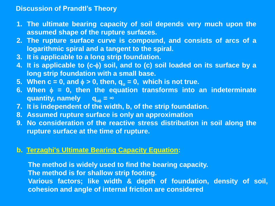
Discussion of Prandtl‘s Theory
1. The ultimate bearing capacity of soil depends very much upon the
assumed shape of the rupture surfaces.
2. The rupture surface curve is compound, and consists of arcs of a
logarithmic spiral and a tangent to the spiral.
3. It is applicable to a long strip foundation.
4. It is applicable to (c-) soil, and to (c) soil loaded on its surface by a
long strip foundation with a small base.
5. When c = 0, and > 0, then, qu = 0, which is not true.
6. When = 0, then the equation transforms into an indeterminate
quantity, namely qu = ∞
7. It is independent of the width, b, of the strip foundation.
8. Assumed rupture surface is only an approximation
9. No consideration of the reactive stress distribution in soil along the
rupture surface at the time of rupture.
b. Terzaghi's Ultimate Bearing Capacity Equation:
The method is widely used to find the bearing capacity.
The method is for shallow strip footing.
Various factors; like width & depth of foundation, density of soil,
cohesion and angle of internal friction are considered
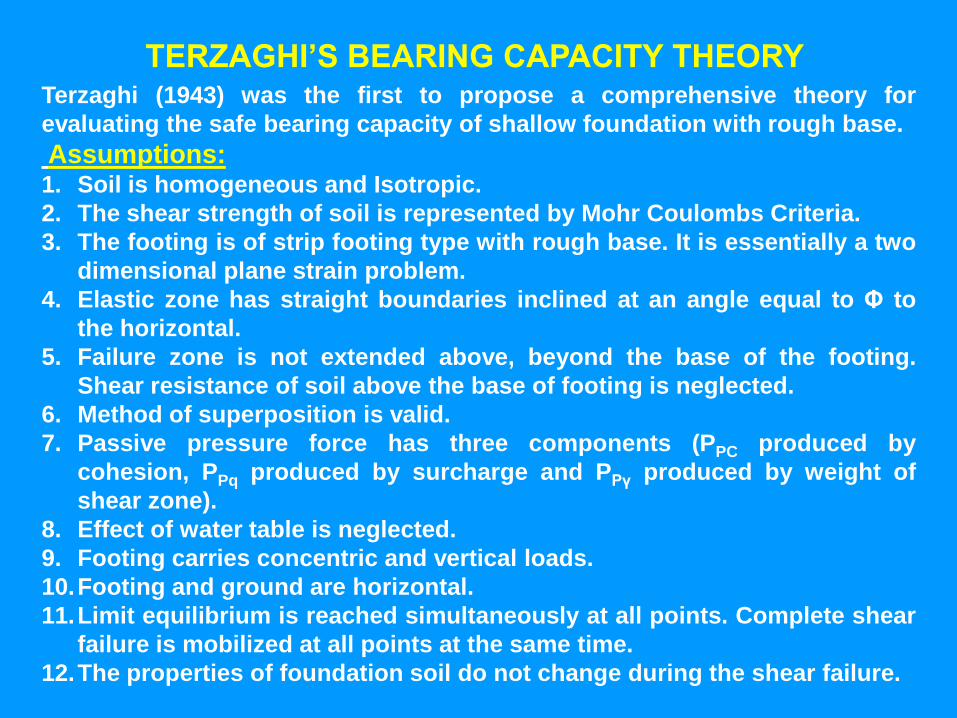
TERZAGHI‘S BEARING CAPACITY THEORYTerzaghi (1943) was the first to propose a comprehensive theory for
evaluating the safe bearing capacity of shallow foundation with rough base.
Assumptions:1. Soil is homogeneous and Isotropic.
2. The shear strength of soil is represented by Mohr Coulombs Criteria.
3. The footing is of strip footing type with rough base. It is essentially a two
dimensional plane strain problem.
4. Elastic zone has straight boundaries inclined at an angle equal to Φ to
the horizontal.
5. Failure zone is not extended above, beyond the base of the footing.
Shear resistance of soil above the base of footing is neglected.
6. Method of superposition is valid.
7. Passive pressure force has three components (PPC produced by
cohesion, PPq produced by surcharge and PPγ produced by weight of
shear zone).
8. Effect of water table is neglected.
9. Footing carries concentric and vertical loads.
10.Footing and ground are horizontal.
11.Limit equilibrium is reached simultaneously at all points. Complete shear
failure is mobilized at all points at the same time.
12.The properties of foundation soil do not change during the shear failure.
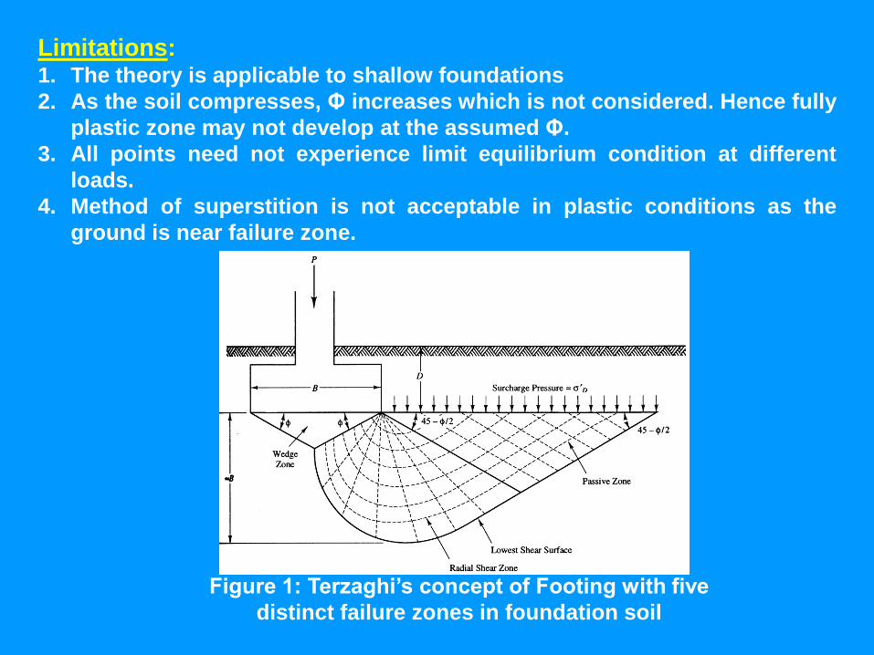
Limitations:1. The theory is applicable to shallow foundations
2. As the soil compresses, Φ increases which is not considered. Hence fully
plastic zone may not develop at the assumed Φ.
3. All points need not experience limit equilibrium condition at different
loads.
4. Method of superstition is not acceptable in plastic conditions as the
ground is near failure zone.
Figure 1: Terzaghi‘s concept of Footing with five
distinct failure zones in foundation soil
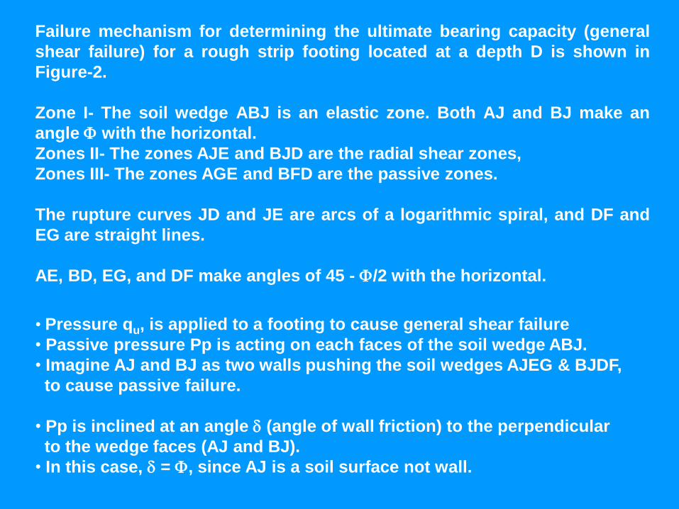
Failure mechanism for determining the ultimate bearing capacity (general
shear failure) for a rough strip footing located at a depth D is shown in
Figure-2.
Zone I- The soil wedge ABJ is an elastic zone. Both AJ and BJ make an
angle with the horizontal.
Zones II- The zones AJE and BJD are the radial shear zones,
Zones III- The zones AGE and BFD are the passive zones.
The rupture curves JD and JE are arcs of a logarithmic spiral, and DF and
EG are straight lines.
AE, BD, EG, and DF make angles of 45 - /2 with the horizontal.
• Pressure qu, is applied to a footing to cause general shear failure
• Passive pressure Pp is acting on each faces of the soil wedge ABJ.
• Imagine AJ and BJ as two walls pushing the soil wedges AJEG & BJDF,
to cause passive failure.
• Pp is inclined at an angle (angle of wall friction) to the perpendicular
to the wedge faces (AJ and BJ).
• In this case, = , since AJ is a soil surface not wall.
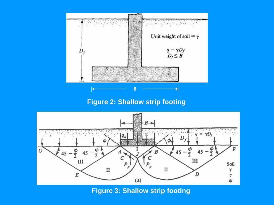
B
Figure 2: Shallow strip footing
Figure 3: Shallow strip footing
cos
cb
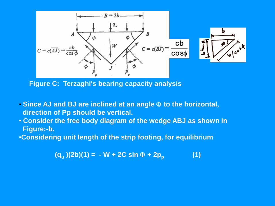
Figure C: Terzaghi's bearing capacity analysis
• Since AJ and BJ are inclined at an angle to the horizontal,
direction of Pp should be vertical.
• Consider the free body diagram of the wedge ABJ as shown in
Figure:-b.
•Considering unit length of the strip footing, for equilibrium
(qu )(2b)(1) = - W + 2C sin + 2pp (1)
Where, b = B/2
W = weight of soil wedge ABJ = b2 tan
C = cohesive force acting along the faces AJ and BJ, and is equal to the
unit cohesion times the length of each face = c (b/cos )
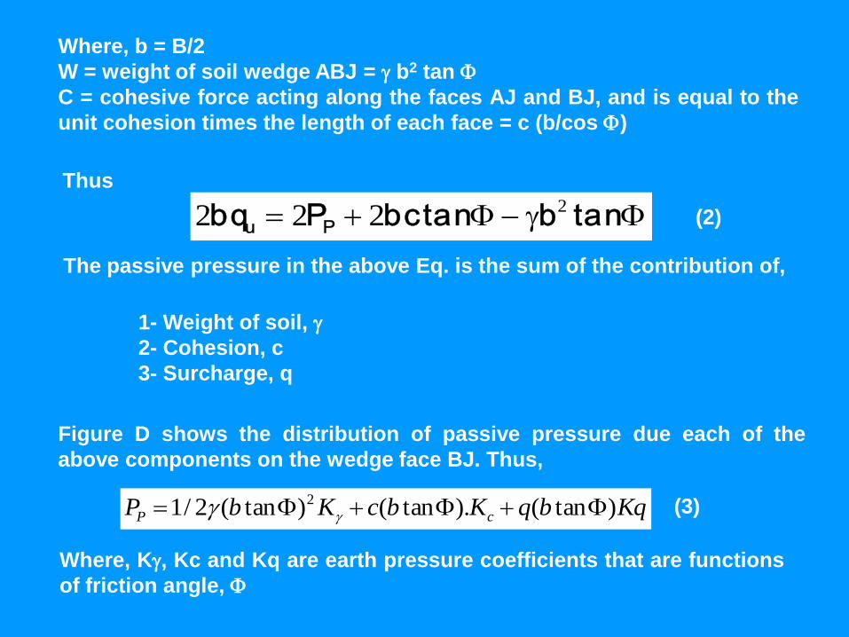
Thus
(2)
The passive pressure in the above Eq. is the sum of the contribution of,
1- Weight of soil,
2- Cohesion, c
3- Surcharge, q
Figure D shows the distribution of passive pressure due each of the
above components on the wedge face BJ. Thus,
(3)
Where, K, Kc and Kq are earth pressure coefficients that are functions
of friction angle,
tanbtanbcPbq Pu
2222
KqbqKbcKbP cP )tan().tan()tan(2/1 2
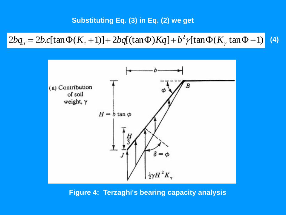
Substituting Eq. (3) in Eq. (2) we get
(4) )1tan([tan])[(tan2)]1([tan.22 2 KbKqbqKcbbq cu
Figure 4: Terzaghi's bearing capacity analysis
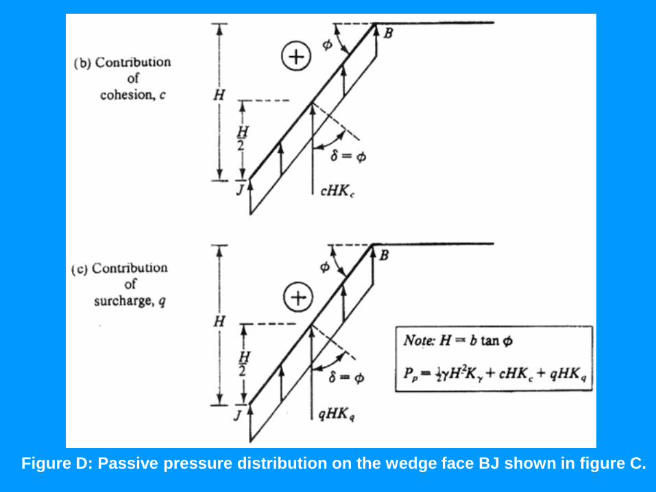
Figure D: Passive pressure distribution on the wedge face BJ shown in figure C.
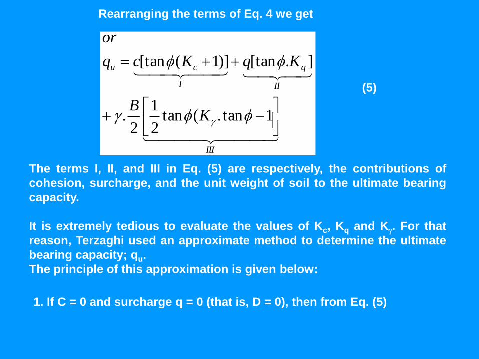
(5)
The terms I, II, and III in Eq. (5) are respectively, the contributions of
cohesion, surcharge, and the unit weight of soil to the ultimate bearing
capacity.
It is extremely tedious to evaluate the values of Kc, Kq and K. For that
reason, Terzaghi used an approximate method to determine the ultimate
bearing capacity; qu.
The principle of this approximation is given below:
1. If C = 0 and surcharge q = 0 (that is, D = 0), then from Eq. (5)
Rearranging the terms of Eq. 4 we get
III
II
q
I
cu
KB
KqKcq
or
1tan.(tan2
1
2.
].[tan)]1([tan
(6)
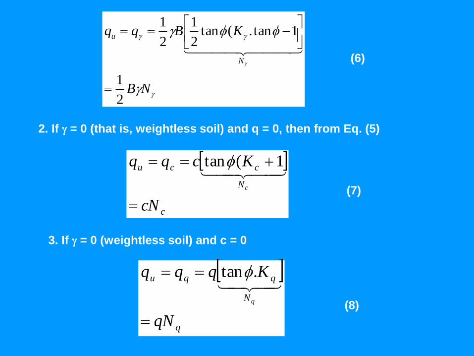
2. If = 0 (that is, weightless soil) and q = 0, then from Eq. (5)
(7)
3. If = 0 (weightless soil) and c = 0
(8)
NB
KBqq
N
u
2
1
1tan.(tan2
1
2
1
c
N
ccu
cN
Kcqq
c
1(tan
q
N
qqu
qN
Kqqq
q
.tan
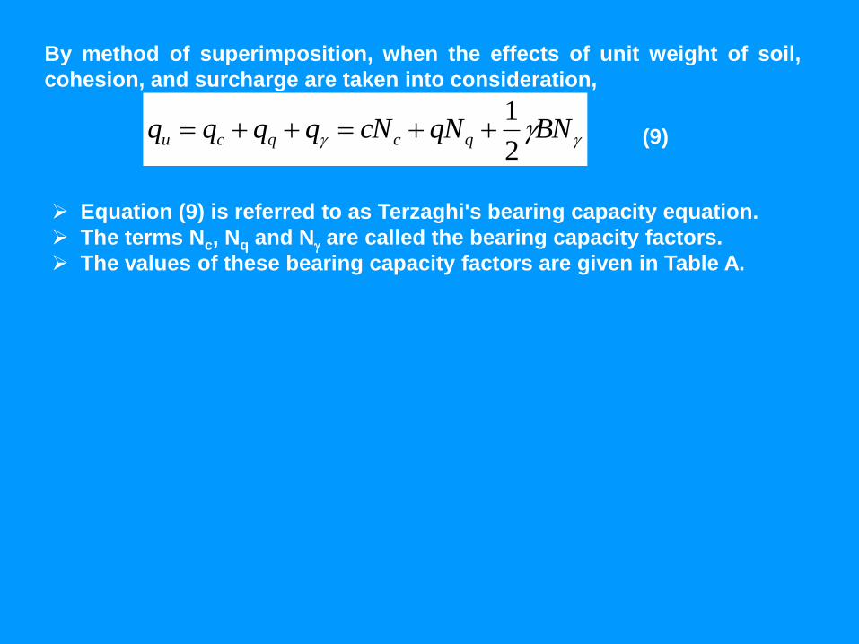
By method of superimposition, when the effects of unit weight of soil,
cohesion, and surcharge are taken into consideration,
(9)
Equation (9) is referred to as Terzaghi's bearing capacity equation.
The terms Nc, Nq and N are called the bearing capacity factors.
The values of these bearing capacity factors are given in Table A.
BNqNcNqqqq qcqcu2
1
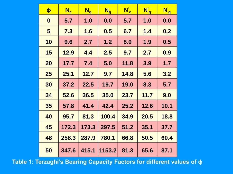
ϕ Nc Nq Ng N'c N'
q N'g
0 5.7 1.0 0.0 5.7 1.0 0.0
5 7.3 1.6 0.5 6.7 1.4 0.2
10 9.6 2.7 1.2 8.0 1.9 0.5
15 12.9 4.4 2.5 9.7 2.7 0.9
20 17.7 7.4 5.0 11.8 3.9 1.7
25 25.1 12.7 9.7 14.8 5.6 3.2
30 37.2 22.5 19.7 19.0 8.3 5.7
34 52.6 36.5 35.0 23.7 11.7 9.0
35 57.8 41.4 42.4 25.2 12.6 10.1
40 95.7 81.3 100.4 34.9 20.5 18.8
45 172.3 173.3 297.5 51.2 35.1 37.7
48 258.3 287.9 780.1 66.8 50.5 60.4
50 347.6 415.1 1153.2 81.3 65.6 87.1
Table 1: Terzaghi‘s Bearing Capacity Factors for different values of ϕ
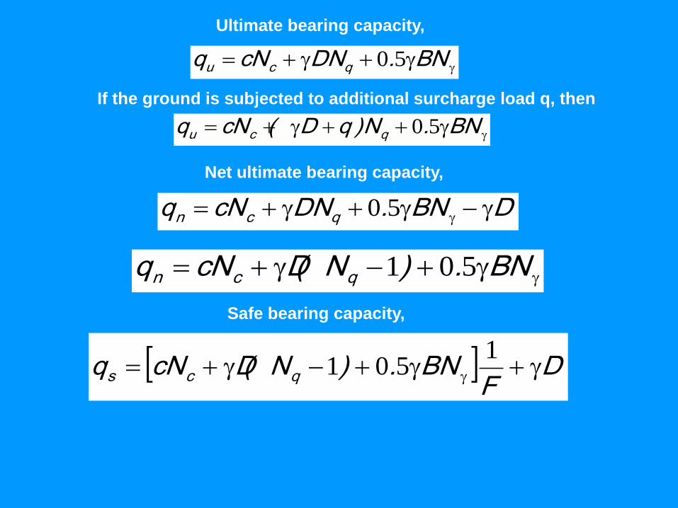
Ultimate bearing capacity,
BN.DNcNq qcu 50
If the ground is subjected to additional surcharge load q, then
BN.N)qD(cNq qcu 50
Net ultimate bearing capacity,
DBN.DNcNq qcn 50
BN.)N(DcNq qcn 501
Safe bearing capacity,
DF
BN.)N(DcNq qcs
1501
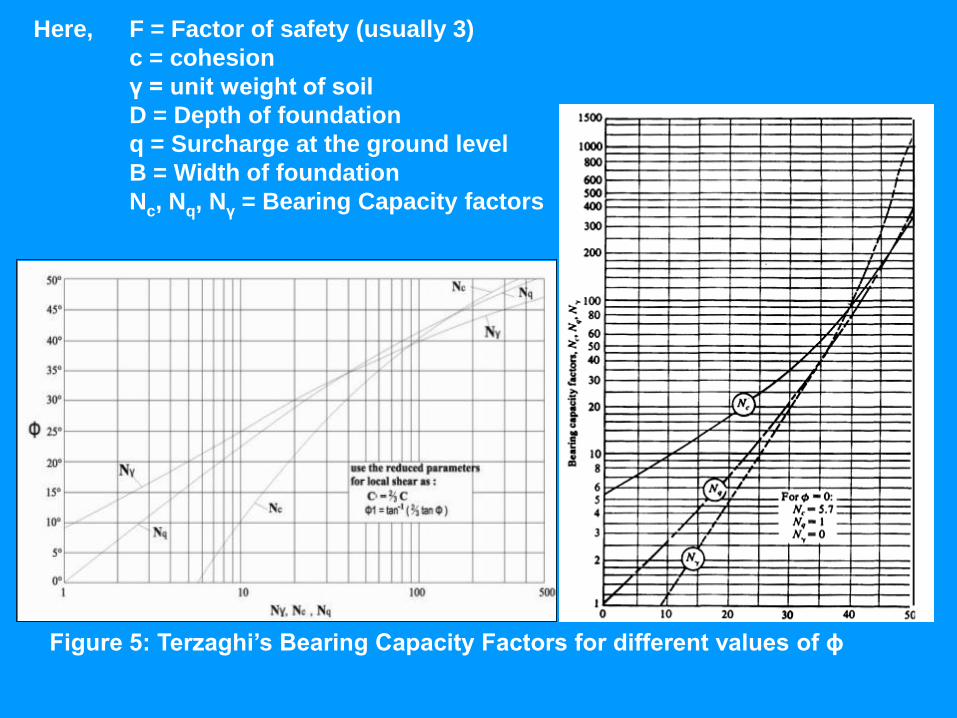
Here, F = Factor of safety (usually 3)
c = cohesion
γ = unit weight of soil
D = Depth of foundation
q = Surcharge at the ground level
B = Width of foundation
Nc, Nq, Nγ = Bearing Capacity factors
Figure 5: Terzaghi‘s Bearing Capacity Factors for different values of ϕ
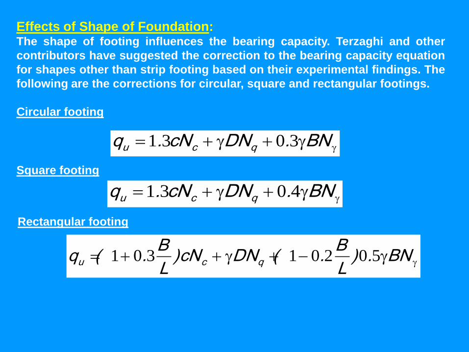
Effects of Shape of Foundation:The shape of footing influences the bearing capacity. Terzaghi and other
contributors have suggested the correction to the bearing capacity equation
for shapes other than strip footing based on their experimental findings. The
following are the corrections for circular, square and rectangular footings.
Circular footing
BN.DNcN.q qcu 3031
Square footing
BN.DNcN.q qcu 4031
Rectangular footing
BN.)L
B.(DNcN)
L
B.(q qcu 50201301
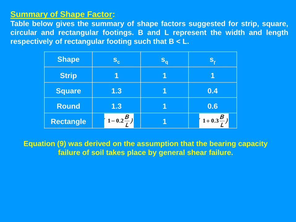
Summary of Shape Factor:Table below gives the summary of shape factors suggested for strip, square,
circular and rectangular footings. B and L represent the width and length
respectively of rectangular footing such that B < L.
Shape sc sq sɼ
Strip 1 1 1
Square 1.3 1 0.4
Round 1.3 1 0.6
Rectangle 1 )L
B.( 301)
L
B.( 201
Equation (9) was derived on the assumption that the bearing capacity
failure of soil takes place by general shear failure.
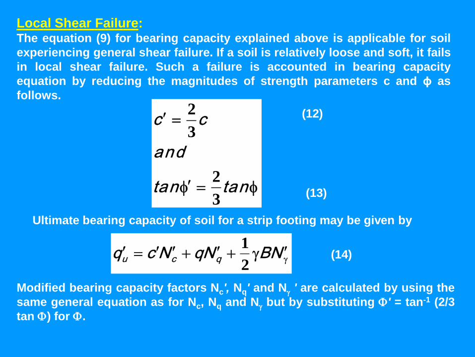
Local Shear Failure:The equation (9) for bearing capacity explained above is applicable for soil
experiencing general shear failure. If a soil is relatively loose and soft, it fails
in local shear failure. Such a failure is accounted in bearing capacity
equation by reducing the magnitudes of strength parameters c and ϕ as
follows.
tantan
and
cc
3
2
3
2 (12)
(13)
Ultimate bearing capacity of soil for a strip footing may be given by
(14) NBNqNcq qcu
2
1
Modified bearing capacity factors Nc', Nq' and N ' are calculated by using the
same general equation as for Nc, Nq and N but by substituting ' = tan-1 (2/3
tan ) for .
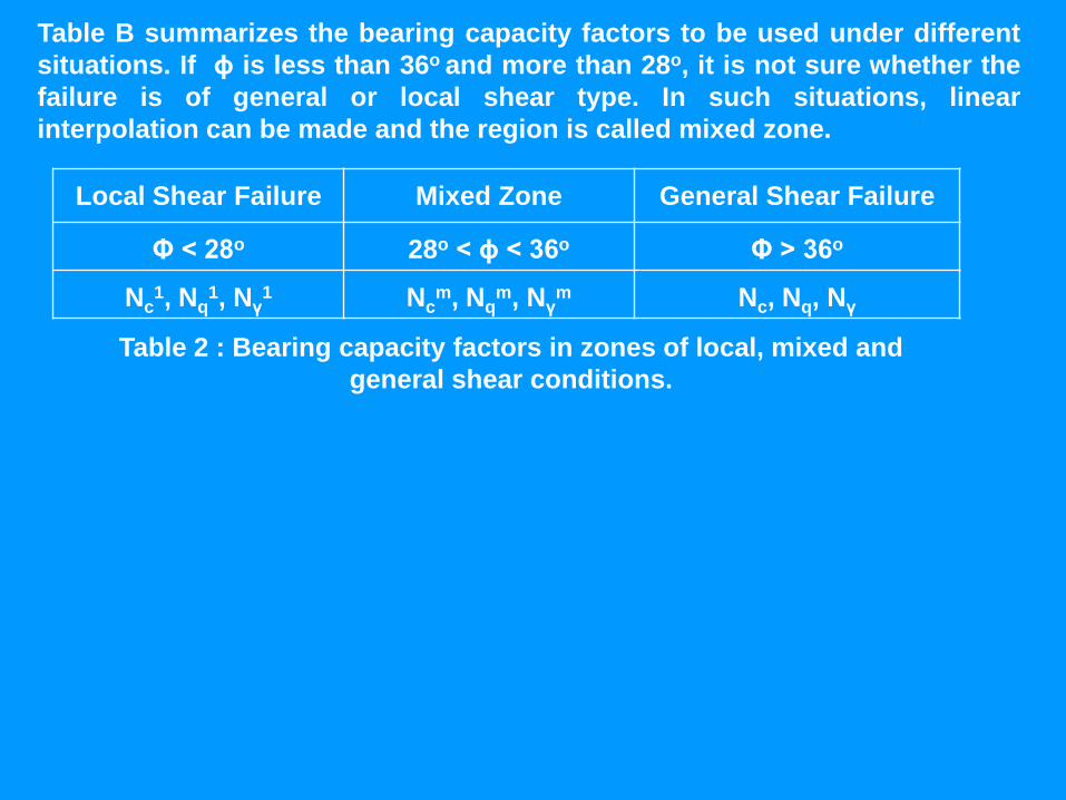
Table B summarizes the bearing capacity factors to be used under different
situations. If ϕ is less than 36o and more than 28o, it is not sure whether the
failure is of general or local shear type. In such situations, linear
interpolation can be made and the region is called mixed zone.
Local Shear Failure Mixed Zone General Shear Failure
Φ < 28o 28o < ϕ < 36o Φ > 36o
Nc1, Nq
1, Nγ1 Nc
m, Nqm, Nγ
m Nc, Nq, Nγ
Table 2 : Bearing capacity factors in zones of local, mixed and
general shear conditions.
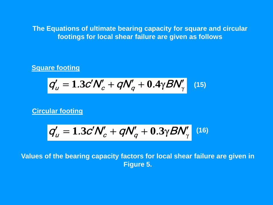
Square footing
(15)
Circular footing
(16)
The Equations of ultimate bearing capacity for square and circular
footings for local shear failure are given as follows
Values of the bearing capacity factors for local shear failure are given in
Figure 5.
NB.NqNc.q qcu 4031
NB.NqNc.q qcu 3031
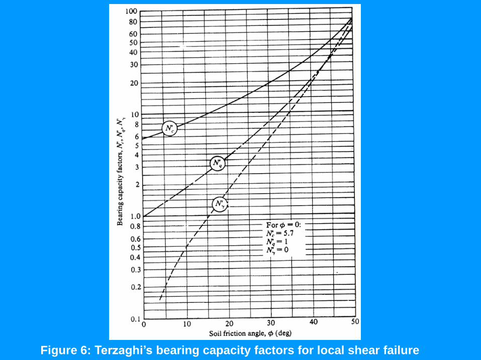
Figure 6: Terzaghi‘s bearing capacity factors for local shear failure
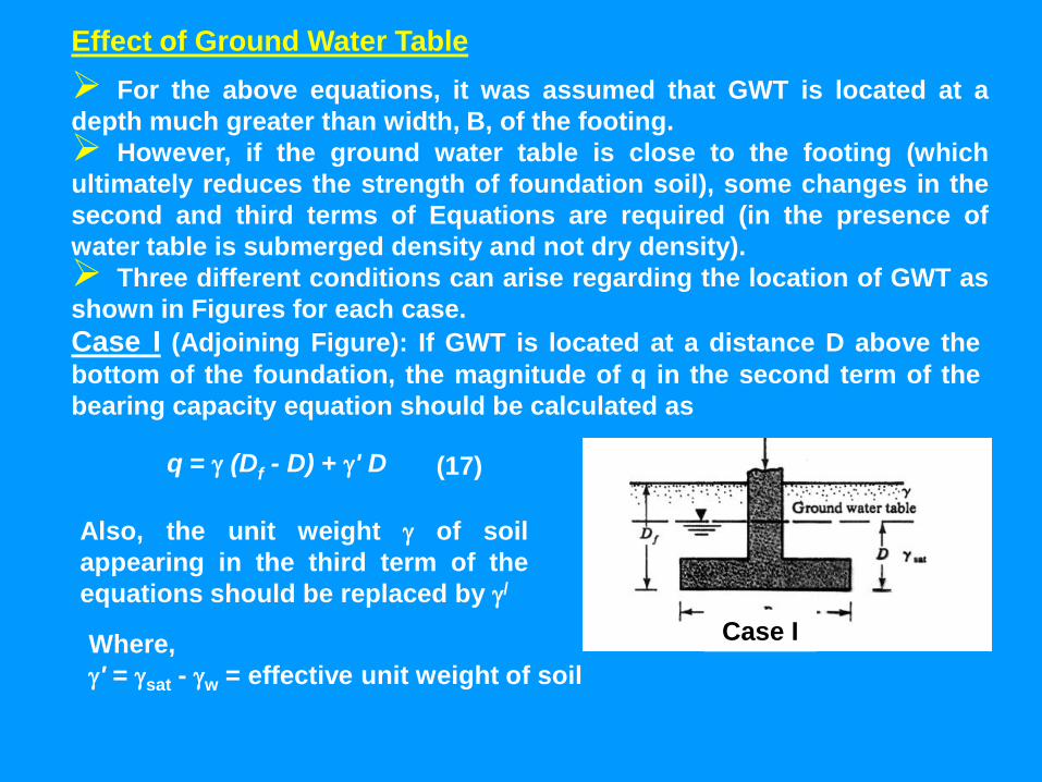
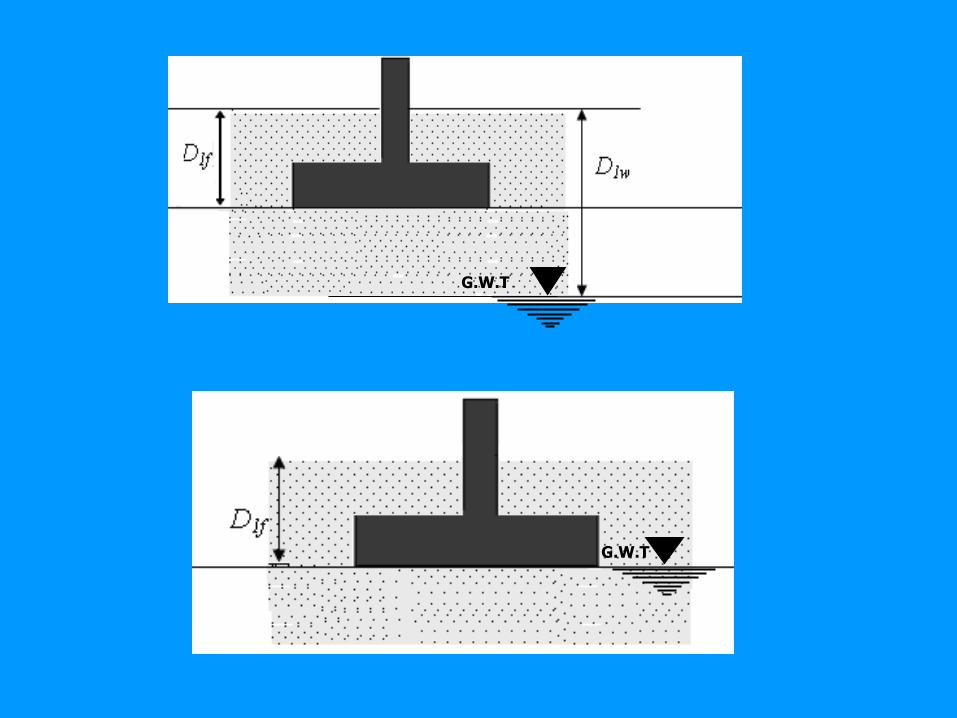
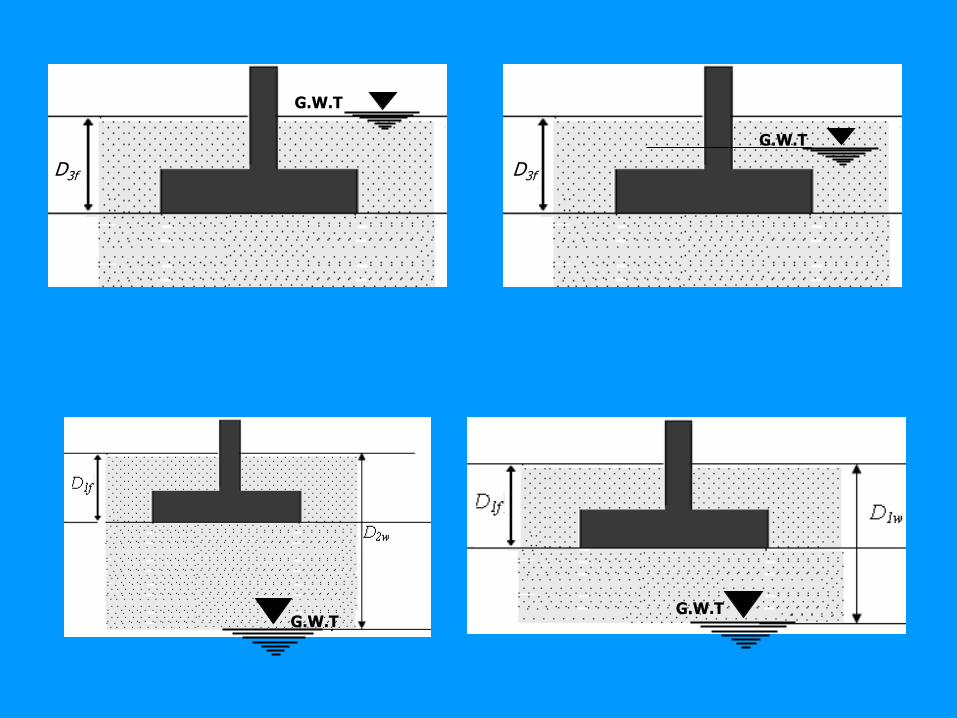
Effect of Ground Water Table
For the above equations, it was assumed that GWT is located at a
depth much greater than width, B, of the footing.
However, if the ground water table is close to the footing (which
ultimately reduces the strength of foundation soil), some changes in the
second and third terms of Equations are required (in the presence of
water table is submerged density and not dry density).
Three different conditions can arise regarding the location of GWT as
shown in Figures for each case.
Case I (Adjoining Figure): If GWT is located at a distance D above the
bottom of the foundation, the magnitude of q in the second term of the
bearing capacity equation should be calculated as
q = (Df - D) + ' D (17)
Also, the unit weight of soil
appearing in the third term of the
equations should be replaced by /
Where,
' = sat - w = effective unit weight of soil
Case I
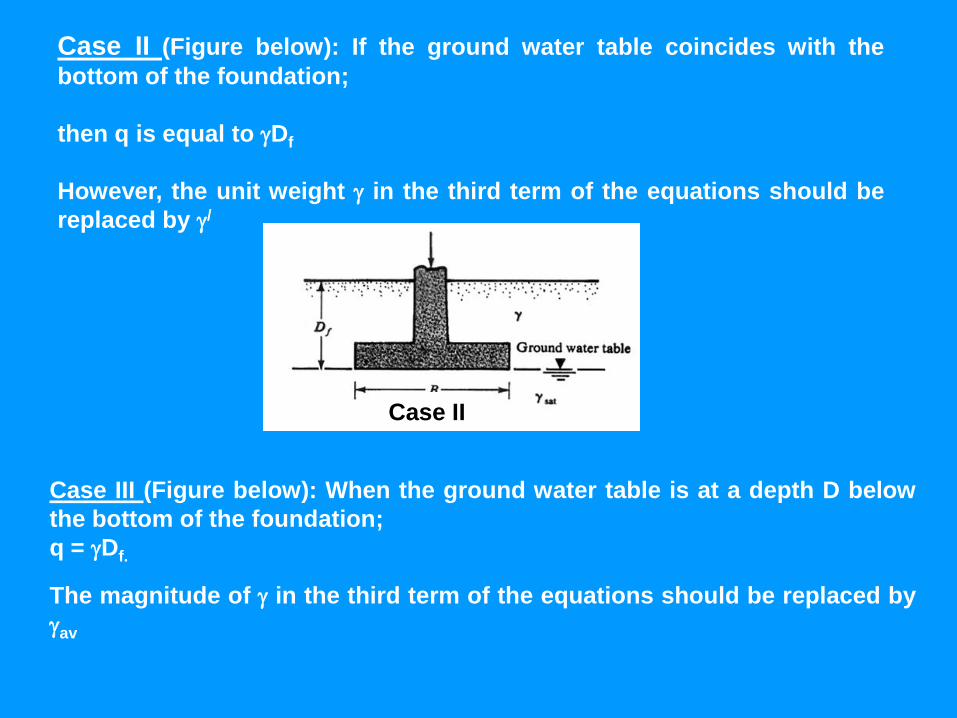
Case II (Figure below): If the ground water table coincides with the
bottom of the foundation;
then q is equal to Df
However, the unit weight in the third term of the equations should be
replaced by /
Case III (Figure below): When the ground water table is at a depth D below
the bottom of the foundation;
q = Df.
The magnitude of in the third term of the equations should be replaced by
av
Case II
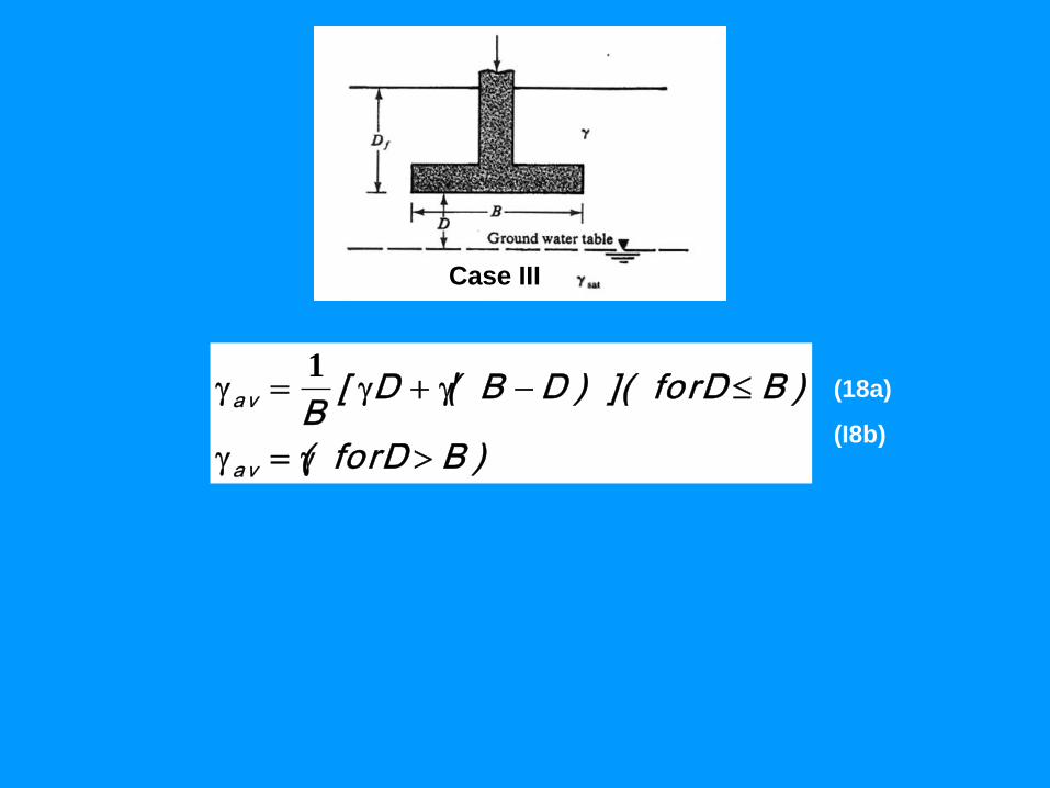
(18a)
(I8b))BforD(
)BforD)](DB(D[B
a v
a v
1
Case III
DZW1
B
Influence o
f R
W1
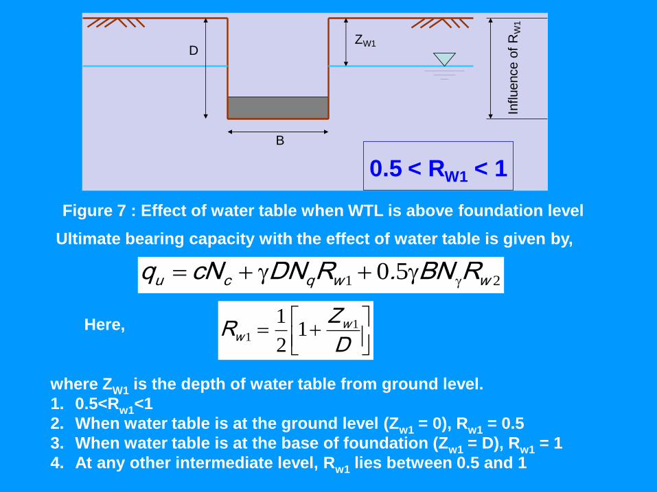
0.5 < RW1 < 1
Figure 7 : Effect of water table when WTL is above foundation level
Ultimate bearing capacity with the effect of water table is given by,
21 50 wwqcu RBN.RDNcNq
Here,
D
ZR w
w1
1 12
1
where ZW1 is the depth of water table from ground level.
1. 0.5<Rw1<1
2. When water table is at the ground level (Zw1 = 0), Rw1 = 0.5
3. When water table is at the base of foundation (Zw1 = D), Rw1 = 1
4. At any other intermediate level, Rw1 lies between 0.5 and 1
DD
ZW2B
Influence o
f R
W2
B
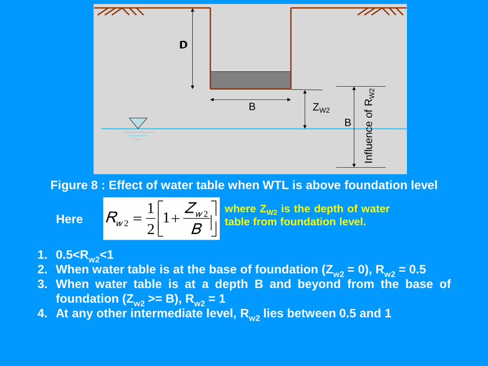
Figure 8 : Effect of water table when WTL is above foundation level
Here
B
ZR w
w2
2 12
1 where ZW2 is the depth of water
table from foundation level.
1. 0.5<Rw2<1
2. When water table is at the base of foundation (Zw2 = 0), Rw2 = 0.5
3. When water table is at a depth B and beyond from the base of
foundation (Zw2 >= B), Rw2 = 1
4. At any other intermediate level, Rw2 lies between 0.5 and 1
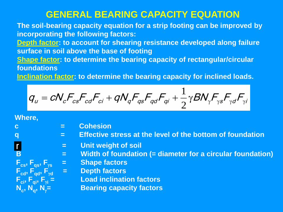
idsqiqdqsqcicdcscu FFFBNFFFqNFFFcNq 2
1
Where,
c = Cohesion
q = Effective stress at the level of the bottom of foundation
ɼ = Unit weight of soil
B = Width of foundation (= diameter for a circular foundation)
Fcs, Fqs, Fs = Shape factors
Fcd, Fqd, Fd = Depth factors
Fci, Fqi, Fi = Load inclination factors
Nc, Nq, N= Bearing capacity factors
GENERAL BEARING CAPACITY EQUATIONThe soil-bearing capacity equation for a strip footing can be improved by
incorporating the following factors:
Depth factor: to account for shearing resistance developed along failure
surface in soil above the base of footing
Shape factor: to determine the bearing capacity of rectangular/circular
foundations
Inclination factor: to determine the bearing capacity for inclined loads.
Terzaghi assumed angle of the failure wedge = ø
While the others assumed the angle as 45+ ø/2,
This results in changes in the values of the bearing capacity factors
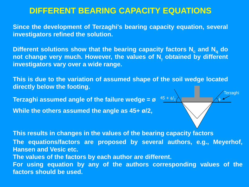
DIFFERENT BEARING CAPACITY EQUATIONS
Since the development of Terzaghi's bearing capacity equation, several
investigators refined the solution.
Different solutions show that the bearing capacity factors Nc and Nq do
not change very much. However, the values of N obtained by different
investigators vary over a wide range.
This is due to the variation of assumed shape of the soil wedge located
directly below the footing.
The equations/factors are proposed by several authors, e.g., Meyerhof,
Hansen and Vesic etc.
The values of the factors by each author are different.
For using equation by any of the authors corresponding values of the
factors should be used.
45 + /2
Terzaghi
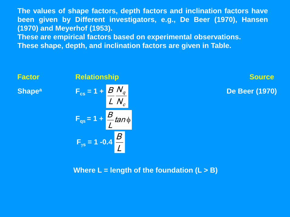
The values of shape factors, depth factors and inclination factors have
been given by Different investigators, e.g., De Beer (1970), Hansen
(1970) and Meyerhof (1953).
These are empirical factors based on experimental observations.
These shape, depth, and inclination factors are given in Table.
Factor Relationship Source
Shapea Fcs = 1 + De Beer (1970)
c
q
N
N
L
B
Fqs = 1 + tanL
B
Fs = 1 -0.4 L
B
Where L = length of the foundation (L > B)
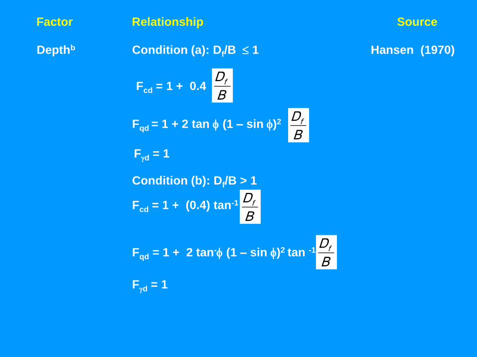
Factor Relationship Source
Depthb Condition (a): Df/B 1 Hansen (1970)
B
Df
Fqd = 1 + 2 tan (1 – sin )2
Fd = 1
Condition (b): Df/B > 1
Fcd = 1 + 0.4
B
Df
Fcd = 1 + (0.4) tan-1
B
Df
Fqd = 1 + 2 tan- (1 – sin )2 tan -1B
Df
Fd = 1
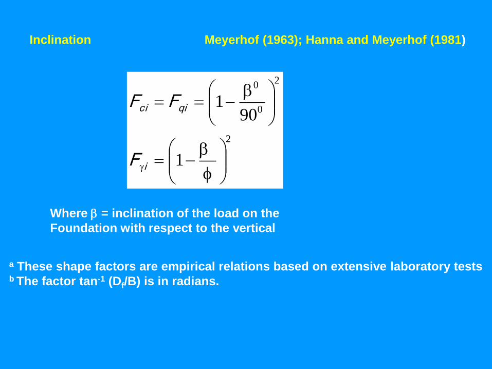
Where = inclination of the load on the
Foundation with respect to the vertical
Inclination Meyerhof (1963); Hanna and Meyerhof (1981)
2
2
0
0
1
901
i
qici
F
FF
a These shape factors are empirical relations based on extensive laboratory testsb The factor tan-1 (Df/B) is in radians.
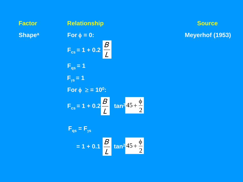
Factor Relationship Source
Shapea For = 0: Meyerhof (1953)
Fcs = 1 + 0.2 tan2
245
Fqs = Fs
L
BFcs = 1 + 0.2
Fqs = 1
Fs = 1
For = 100:
L
B
= 1 + 0.1 tan2
245
L
B
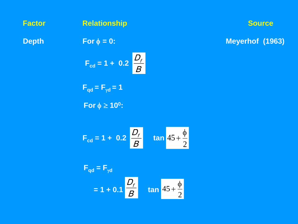
Factor Relationship Source
Depth For = 0: Meyerhof (1963)
B
Df
Fqd = Fd = 1
For 100:
Fcd = 1 + 0.2
Fcd = 1 + 0.2 tanB
Df
245
Fqd = Fd
= 1 + 0.1 tan 2
45
B
Df
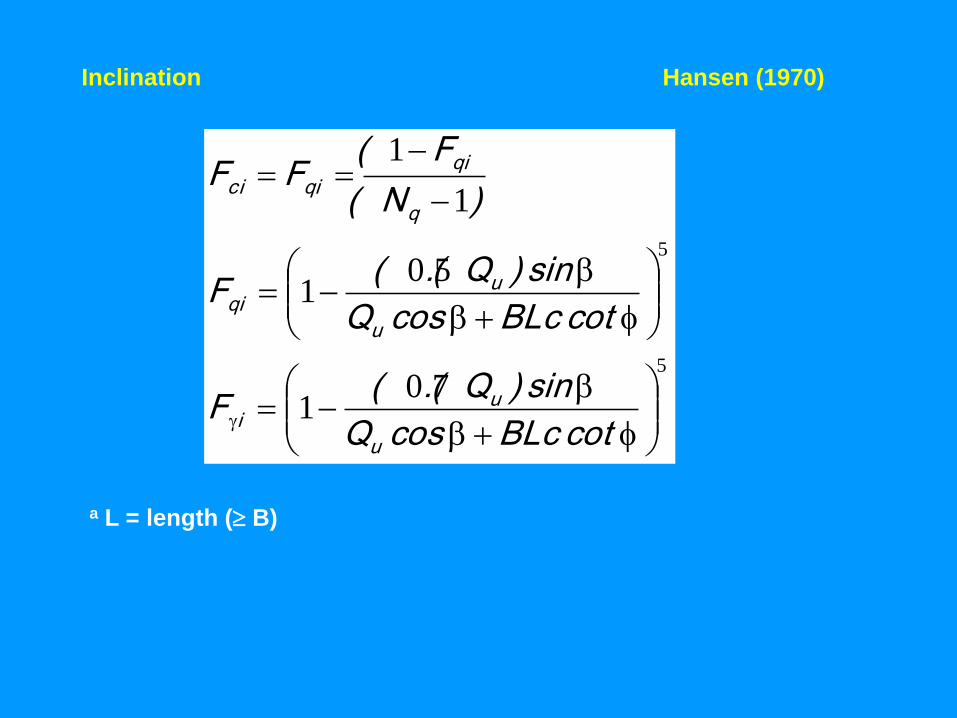
Inclination Hansen (1970)
5
5
701
501
1
1
cotBLccosQ
sin)Q(.(F
cotBLccosQ
sin)Q(.(F
)N(
F(FF
u
ui
u
uqi
q
qiqici
a L = length ( B)
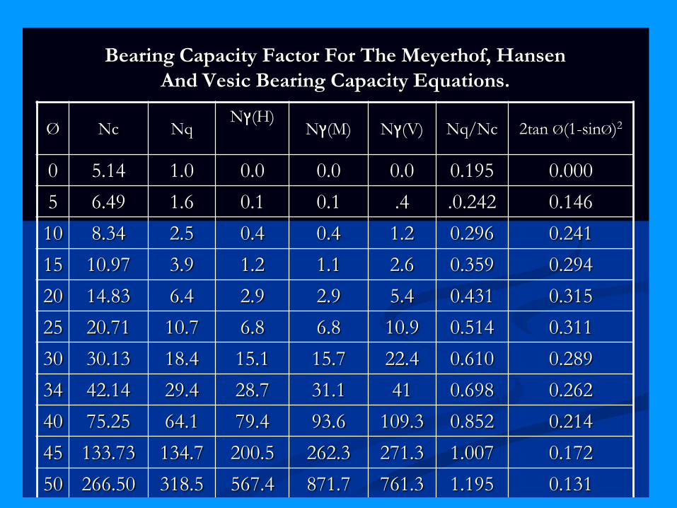
Bearing Capacity Factor For The Meyerhof, Hansen
And Vesic Bearing Capacity Equations.
Ø Nc NqN (H)
N (M) N (V) Nq/Nc 2tan Ø(1-sinØ)2
0 5.14 1.0 0.0 0.0 0.0 0.195 0.000
5 6.49 1.6 0.1 0.1 .4 .0.242 0.146
10 8.34 2.5 0.4 0.4 1.2 0.296 0.241
15 10.97 3.9 1.2 1.1 2.6 0.359 0.294
20 14.83 6.4 2.9 2.9 5.4 0.431 0.315
25 20.71 10.7 6.8 6.8 10.9 0.514 0.311
30 30.13 18.4 15.1 15.7 22.4 0.610 0.289
34 42.14 29.4 28.7 31.1 41 0.698 0.262
40 75.25 64.1 79.4 93.6 109.3 0.852 0.214
45 133.73 134.7 200.5 262.3 271.3 1.007 0.172
50 266.50 318.5 567.4 871.7 761.3 1.195 0.131
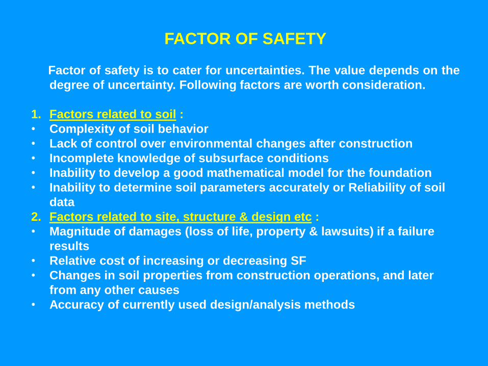
FACTOR OF SAFETY
Factor of safety is to cater for uncertainties. The value depends on the
degree of uncertainty. Following factors are worth consideration.
1. Factors related to soil :
• Complexity of soil behavior
• Lack of control over environmental changes after construction
• Incomplete knowledge of subsurface conditions
• Inability to develop a good mathematical model for the foundation
• Inability to determine soil parameters accurately or Reliability of soil
data
2. Factors related to site, structure & design etc :
• Magnitude of damages (loss of life, property & lawsuits) if a failure
results
• Relative cost of increasing or decreasing SF
• Changes in soil properties from construction operations, and later
from any other causes
• Accuracy of currently used design/analysis methods
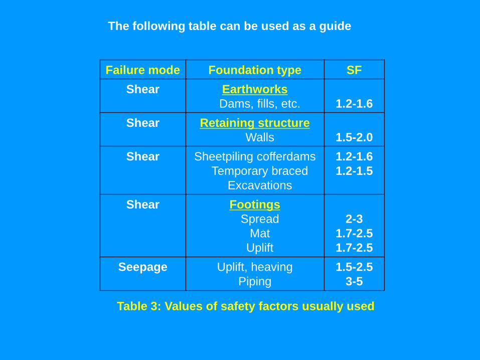
The following table can be used as a guide
Table 3: Values of safety factors usually used
Failure mode Foundation type SF
Shear Earthworks
Dams, fills, etc. 1.2-1.6
Shear Retaining structure
Walls 1.5-2.0
Shear Sheetpiling cofferdams
Temporary braced
Excavations
1.2-1.6
1.2-1.5
Shear Footings
Spread
Mat
Uplift
2-3
1.7-2.5
1.7-2.5
Seepage Uplift, heaving
Piping
1.5-2.5
3-5
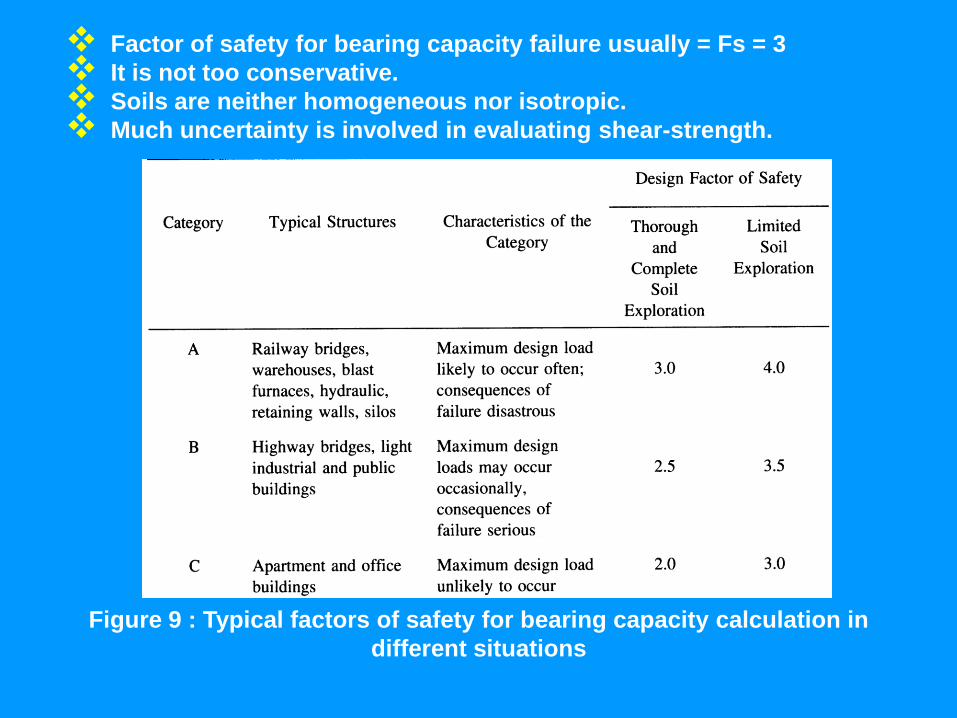
Factor of safety for bearing capacity failure usually = Fs = 3
It is not too conservative.
Soils are neither homogeneous nor isotropic.
Much uncertainty is involved in evaluating shear-strength.
Figure 9 : Typical factors of safety for bearing capacity calculation in
different situations
DETERMINATION OF BEARING CAPACITY FROM FIELD
TESTS
Field Tests are performed in the field. You have understood the
advantages of field tests over laboratory tests for obtaining the desired
property of soil. The biggest advantages are that there is no need to
extract soil sample and the conditions during testing are identical to the
actual situation.
Major advantages of field tests are
1. Sampling is not required
2. Soil disturbance is minimum
Major disadvantages of field tests are
1. Laborious
2. Time consuming
3. Heavy equipment to be carried to field
4. Short duration behavior
The most commonly tests ,used for estimating the bearing capacity of
soil, are;
I. Plate load test
II. Standard Penetration test
III. Cone penetration test
PLATE LOAD TEST FOR BEARING CAPACITY OF SOIL
(AASHTO: T 235 – 96), (ASTM: D 1194 – 94)
It is also known as Field load test or Static load test. The test method has
been withdrawn by the ASTM committee since December 2000.
It is the most reliable method of obtaining the ultimate bearing capacity if
the load test is on a full-size footing; however, this is not possible. The
usual practice is to load test plates of diameters 30-cm to 75-cm.These
sizes are usually too small to extrapolate to full-size footings.
Several factors ,such as:
1. The test gives information about soil to a depth of 2D only,
2. Does not fully take into account the time effect which causes the
extrapolation to be questionable.
For such reasons ASTM has deleted the test since 2000.
1. APPARATUS:
1.1 Loading platform of sufficient size and strength to supply the
estimated load.
1.2 Hydraulic or mechanical jack of sufficient capacity to provide the
maximum estimated load for the soil conditions involved, but not
less than 50-tons
1.3 Bearing plates: Three circular steel bearing plates, not less than
1-in (25-mm) in thickness and varying in diameter from 12-in
(30-cm) to 30-in (75-cm).
1.4 Settlement recording devices such as dial gauges to measure
settlement to an accuracy of at least 0.01-in (0.25-mm).
1.5 Equipment required for making test pit & loading arrangement.
2. PROCEDURE:
2.1 Selection of test areas: Perform the load test at the proposed
footing level and under the same conditions to which the proposed
footing will be subjected.
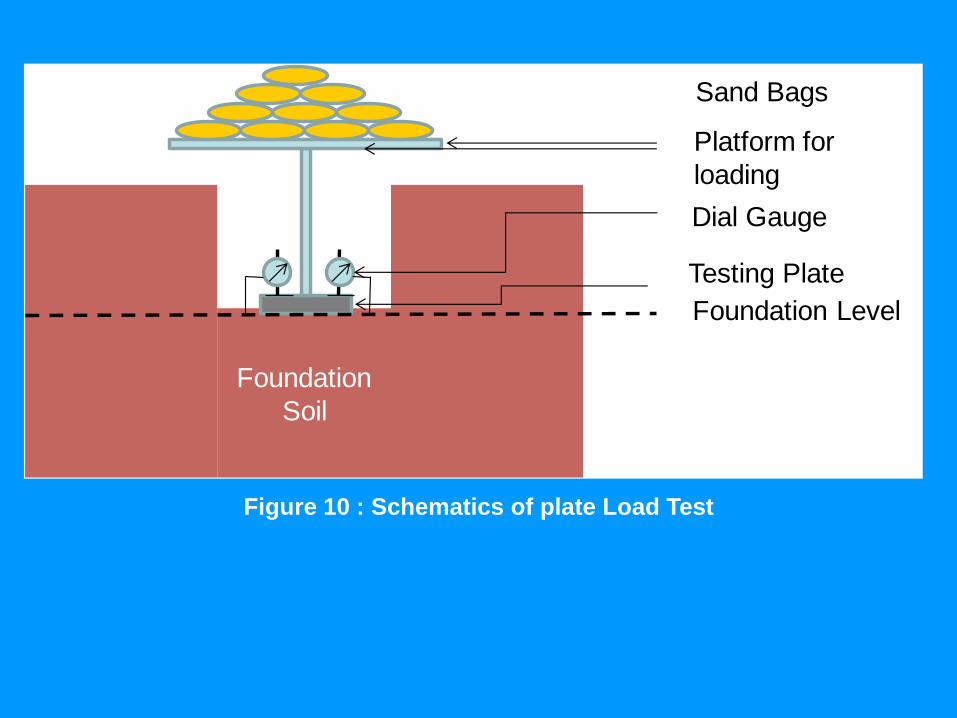
Foundation
Soil
Sand Bags
Platform for
loading
Foundation Level
Testing Plate
Dial Gauge
Figure 10 : Schematics of plate Load Test
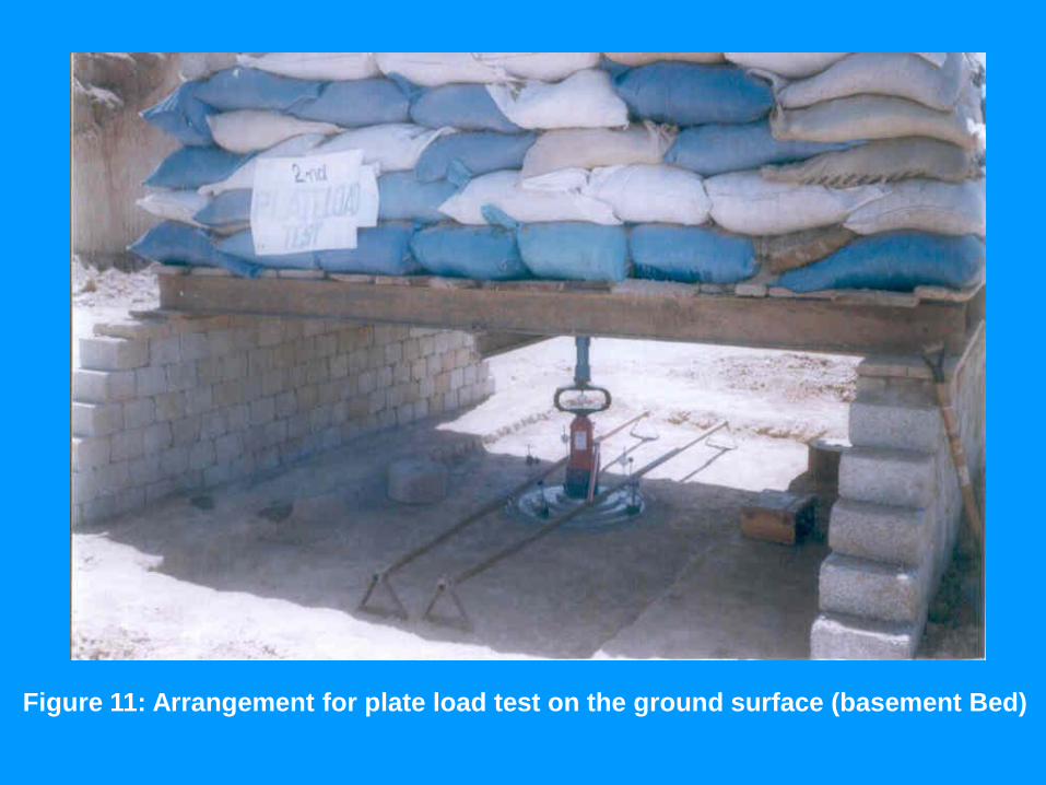
Figure 11: Arrangement for plate load test on the ground surface (basement Bed)
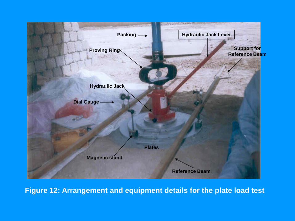
Reference Beam
Support for
Reference Beam
Hydraulic Jack Lever
Hydraulic Jack
Plates
Dial Gauge
Proving Ring
Packing
Magnetic stand
Figure 12: Arrangement and equipment details for the plate load test
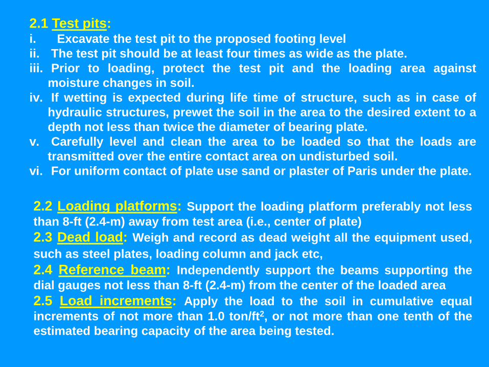
2.1 Test pits:i. Excavate the test pit to the proposed footing level
ii. The test pit should be at least four times as wide as the plate.
iii. Prior to loading, protect the test pit and the loading area against
moisture changes in soil.
iv. If wetting is expected during life time of structure, such as in case of
hydraulic structures, prewet the soil in the area to the desired extent to a
depth not less than twice the diameter of bearing plate.
v. Carefully level and clean the area to be loaded so that the loads are
transmitted over the entire contact area on undisturbed soil.
vi. For uniform contact of plate use sand or plaster of Paris under the plate.
2.2 Loading platforms: Support the loading platform preferably not less
than 8-ft (2.4-m) away from test area (i.e., center of plate)
2.3 Dead load: Weigh and record as dead weight all the equipment used,
such as steel plates, loading column and jack etc,
2.4 Reference beam: Independently support the beams supporting the
dial gauges not less than 8-ft (2.4-m) from the center of the loaded area
2.5 Load increments: Apply the load to the soil in cumulative equal
increments of not more than 1.0 ton/ft2, or not more than one tenth of the
estimated bearing capacity of the area being tested.
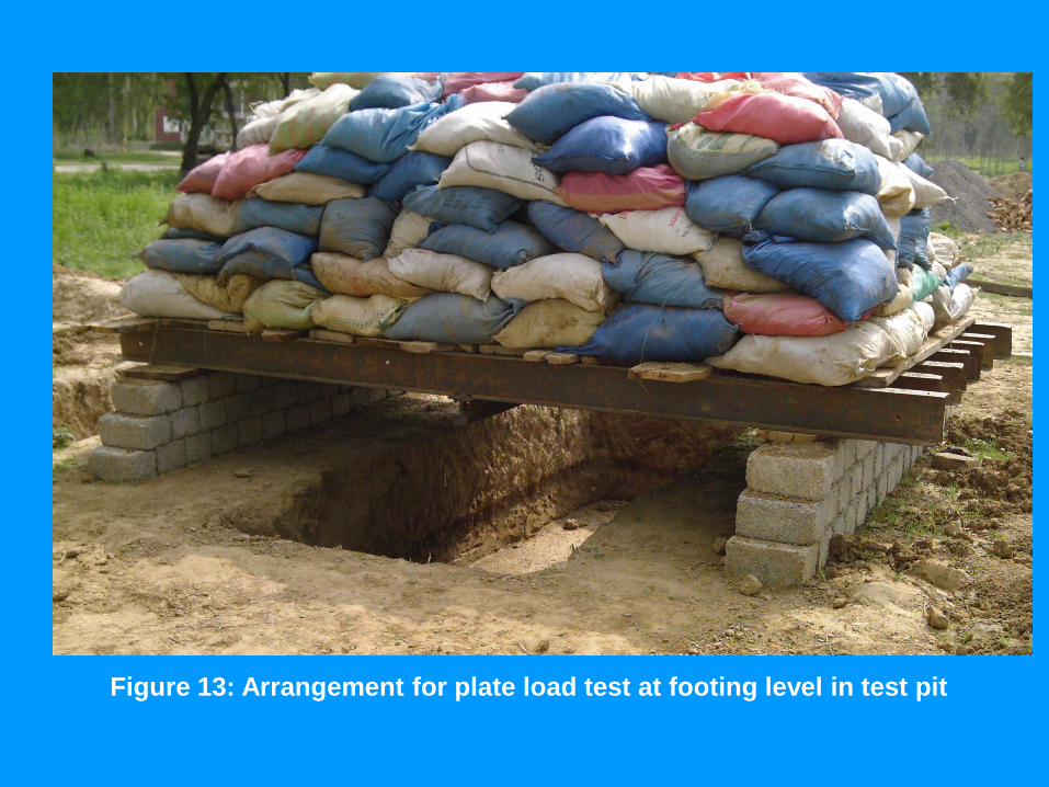
Figure 13: Arrangement for plate load test at footing level in test pit
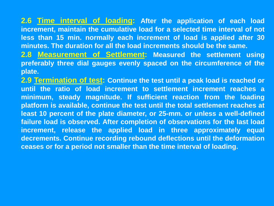
2.6 Time interval of loading: After the application of each load
increment, maintain the cumulative load for a selected time interval of not
less than 15 min. normally each increment of load is applied after 30
minutes. The duration for all the load increments should be the same.
2.8 Measurement of Settlement: Measured the settlement using
preferably three dial gauges evenly spaced on the circumference of the
plate.
2.9 Termination of test: Continue the test until a peak load is reached or
until the ratio of load increment to settlement increment reaches a
minimum, steady magnitude. If sufficient reaction from the loading
platform is available, continue the test until the total settlement reaches at
least 10 percent of the plate diameter, or 25-mm. or unless a well-defined
failure load is observed. After completion of observations for the last load
increment, release the applied load in three approximately equal
decrements. Continue recording rebound deflections until the deformation
ceases or for a period not smaller than the time interval of loading.
3. REPORT :
In addition to recording the time, load, and settlement data, report all
associated conditions and observations pertaining to the test, including
the following:
1. Date
2. List of personnel
3. Weather conditions
4. Air temperature at time of load increments and
5. Irregularity in routine procedure if any.
4. CALCULATIONS:
a. Draw a graph showing relation between (stress & time) and
(settlement & time).
b. Draw another graph between stress & settlement with stress at
ordinate and settlement at abscissa. From the stress-settlement graph,
the ultimate bearing capacity (σu) is taken as shown in Fig. 1, and the
allowable bearing capacity (σa) is determined by:
σa = σu / F.O.S
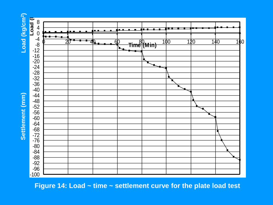
Plate Load Test
-100-96-92-88-84-80-76-72-68-64-60-56-52-48-44-40-36-32-28-24-20-16-12-8-4048
0 20 40 60 80 100 120 140 160Time (Min)
Lo
ad
(kg
/cm
2)
Sett
lem
en
t (m
m)
Lo
ad
(kg
/cm
2)
Figure 14: Load ~ time ~ settlement curve for the plate load test
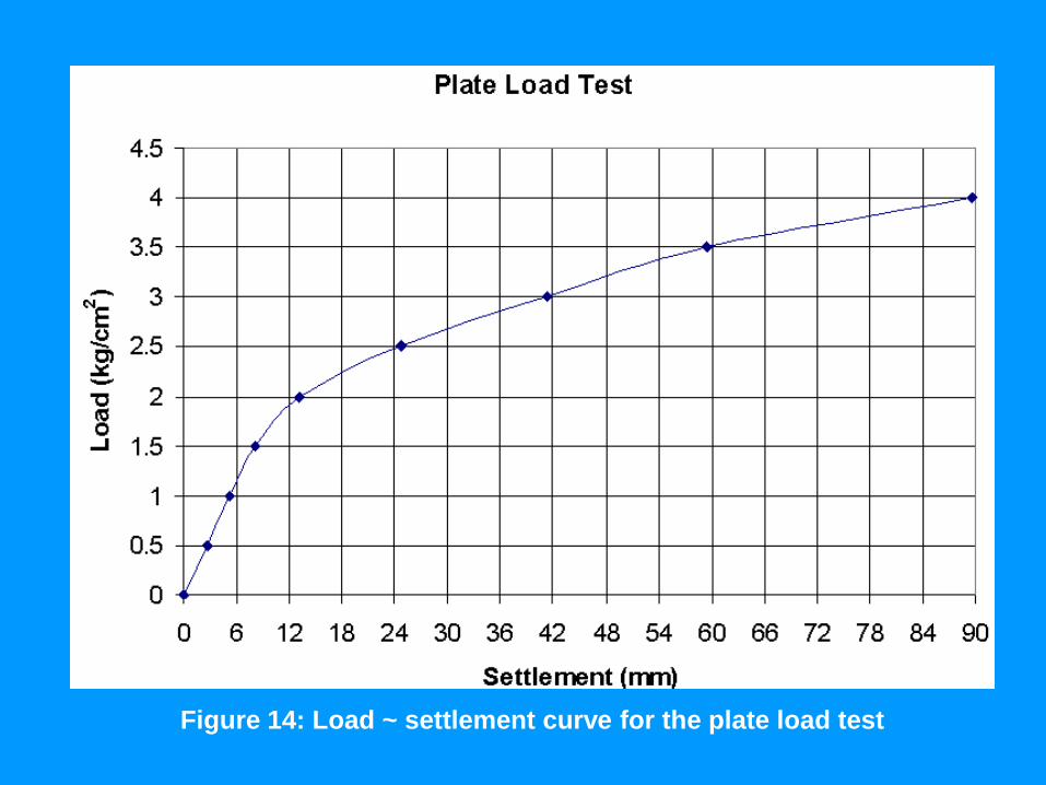
Figure 14: Load ~ settlement curve for the plate load test
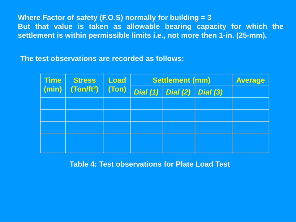
Where Factor of safety (F.O.S) normally for building = 3
But that value is taken as allowable bearing capacity for which the
settlement is within permissible limits i.e., not more then 1-in. (25-mm).
The test observations are recorded as follows:
Time
(min)
Stress
(Ton/ft2)
Load
(Ton)
Settlement (mm) Average
Dial (1) Dial (2) Dial (3)
Table 4: Test observations for Plate Load Test
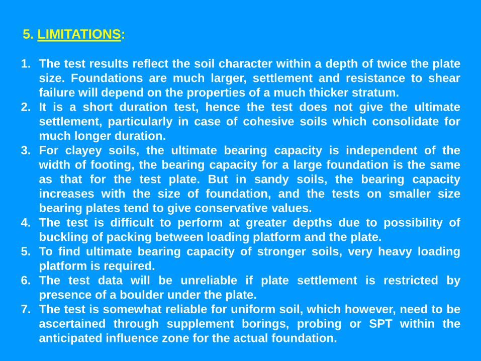
1. The test results reflect the soil character within a depth of twice the plate
size. Foundations are much larger, settlement and resistance to shear
failure will depend on the properties of a much thicker stratum.
2. It is a short duration test, hence the test does not give the ultimate
settlement, particularly in case of cohesive soils which consolidate for
much longer duration.
3. For clayey soils, the ultimate bearing capacity is independent of the
width of footing, the bearing capacity for a large foundation is the same
as that for the test plate. But in sandy soils, the bearing capacity
increases with the size of foundation, and the tests on smaller size
bearing plates tend to give conservative values.
4. The test is difficult to perform at greater depths due to possibility of
buckling of packing between loading platform and the plate.
5. To find ultimate bearing capacity of stronger soils, very heavy loading
platform is required.
6. The test data will be unreliable if plate settlement is restricted by
presence of a boulder under the plate.
7. The test is somewhat reliable for uniform soil, which however, need to be
ascertained through supplement borings, probing or SPT within the
anticipated influence zone for the actual foundation.
5. LIMITATIONS:
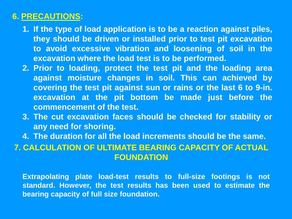
6. PRECAUTIONS:
1. If the type of load application is to be a reaction against piles,
they should be driven or installed prior to test pit excavation
to avoid excessive vibration and loosening of soil in the
excavation where the load test is to be performed.
2. Prior to loading, protect the test pit and the loading area
against moisture changes in soil. This can achieved by
covering the test pit against sun or rains or the last 6 to 9-in.
excavation at the pit bottom be made just before the
commencement of the test.
3. The cut excavation faces should be checked for stability or
any need for shoring.
4. The duration for all the load increments should be the same.
7. CALCULATION OF ULTIMATE BEARING CAPACITY OF ACTUAL
FOUNDATION
Extrapolating plate load-test results to full-size footings is not
standard. However, the test results has been used to estimate the
bearing capacity of full size foundation.
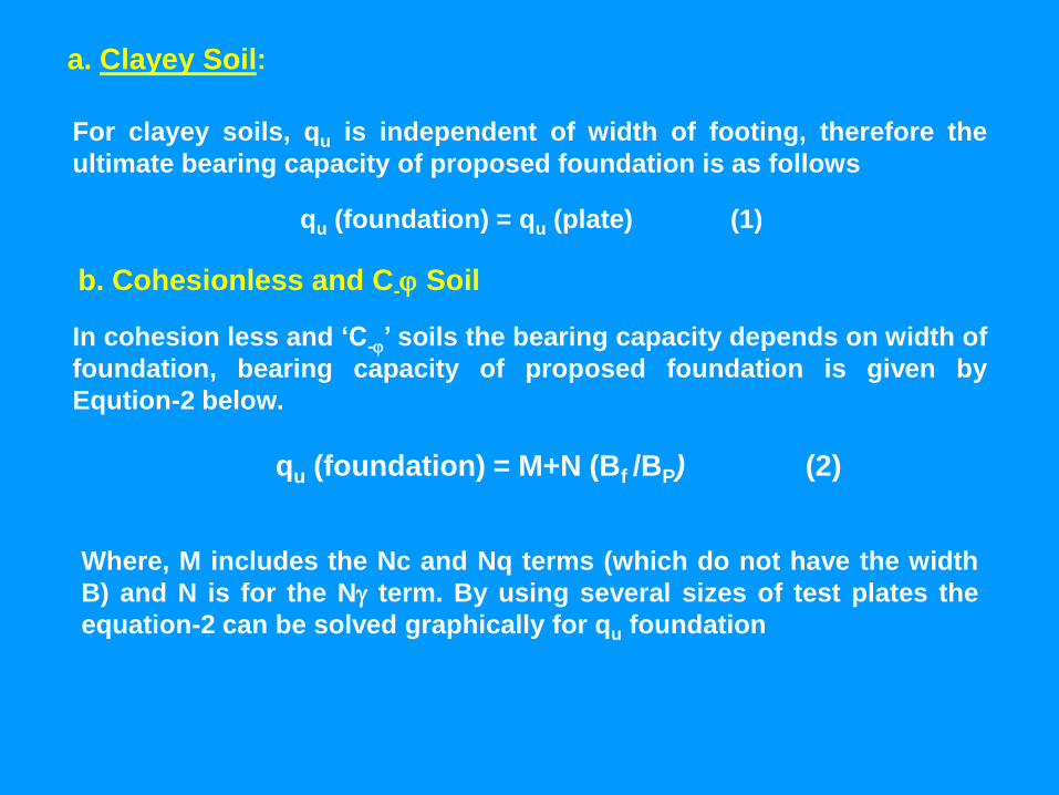
a. Clayey Soil:
For clayey soils, qu is independent of width of footing, therefore the
ultimate bearing capacity of proposed foundation is as follows
qu (foundation) = qu (plate) (1)
b. Cohesionless and C- Soil
In cohesion less and ‗C-‘ soils the bearing capacity depends on width of
foundation, bearing capacity of proposed foundation is given by
Eqution-2 below.
qu (foundation) = M+N (Bf /BP) (2)
Where, M includes the Nc and Nq terms (which do not have the width
B) and N is for the N term. By using several sizes of test plates the
equation-2 can be solved graphically for qu foundation
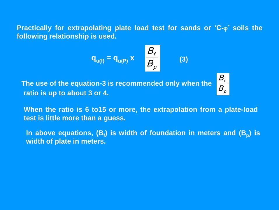
Practically for extrapolating plate load test for sands or ‗C-‘ soils the
following relationship is used.
qu(f) = qu(P) x p
f
B
B(3)
The use of the equation-3 is recommended only when the p
f
B
B
ratio is up to about 3 or 4.
When the ratio is 6 to15 or more, the extrapolation from a plate-load
test is little more than a guess.
In above equations, (Bf) is width of foundation in meters and (Bp) is
width of plate in meters.
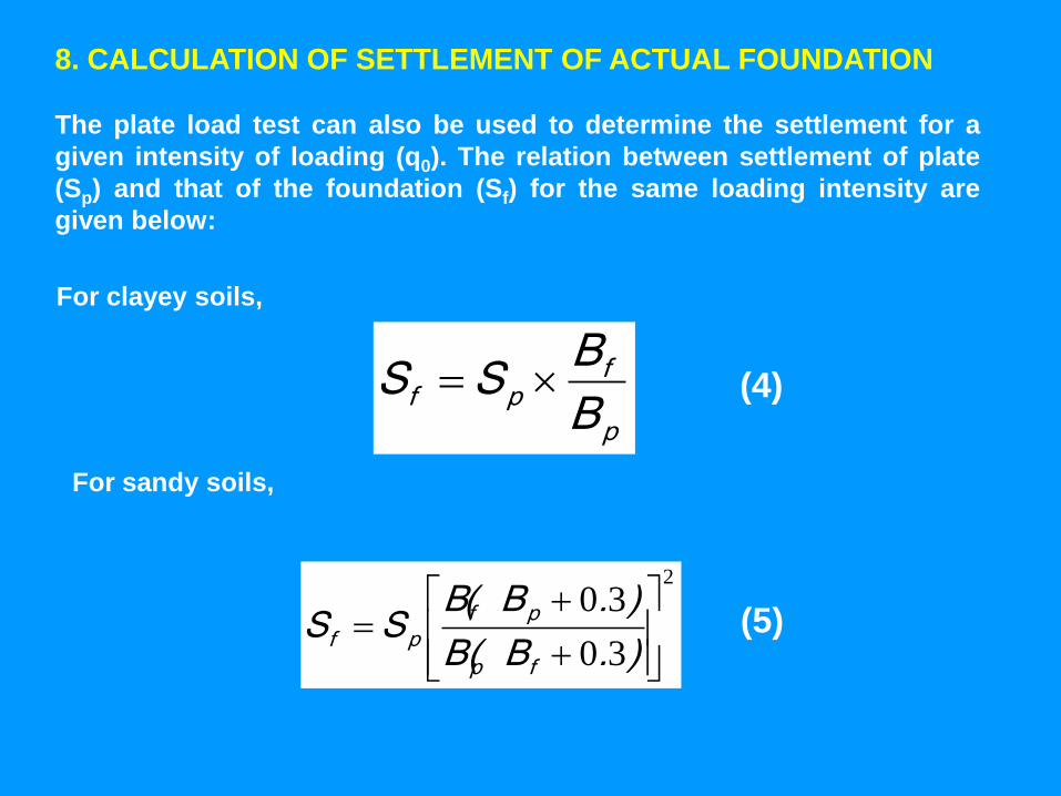
8. CALCULATION OF SETTLEMENT OF ACTUAL FOUNDATION
The plate load test can also be used to determine the settlement for a
given intensity of loading (q0). The relation between settlement of plate
(Sp) and that of the foundation (Sf) for the same loading intensity are
given below:
For clayey soils,
p
fpf
B
BSS (4)
For sandy soils,
2
30
30
).B(B
).B(BSS
fp
pfpf
(5)
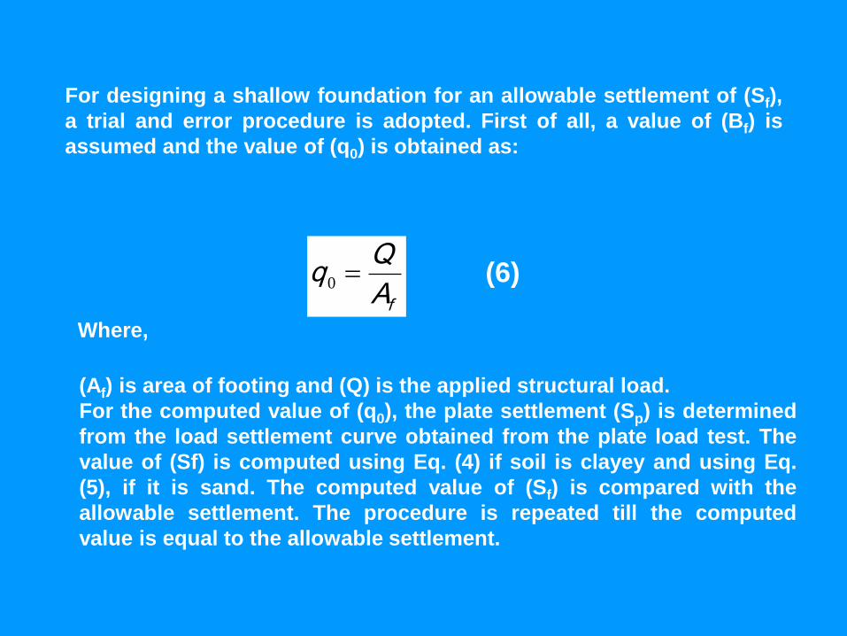
For designing a shallow foundation for an allowable settlement of (Sf),
a trial and error procedure is adopted. First of all, a value of (Bf) is
assumed and the value of (q0) is obtained as:
fA
Qq 0 (6)
Where,
(Af) is area of footing and (Q) is the applied structural load.
For the computed value of (q0), the plate settlement (Sp) is determined
from the load settlement curve obtained from the plate load test. The
value of (Sf) is computed using Eq. (4) if soil is clayey and using Eq.
(5), if it is sand. The computed value of (Sf) is compared with the
allowable settlement. The procedure is repeated till the computed
value is equal to the allowable settlement.
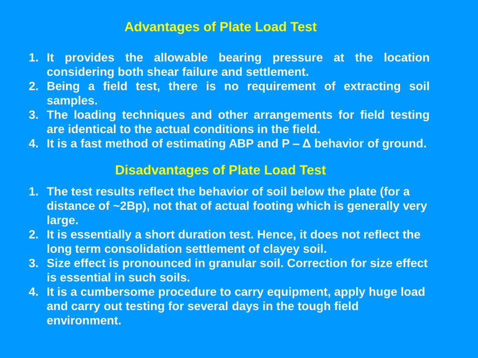
Advantages of Plate Load Test
1. It provides the allowable bearing pressure at the location
considering both shear failure and settlement.
2. Being a field test, there is no requirement of extracting soil
samples.
3. The loading techniques and other arrangements for field testing
are identical to the actual conditions in the field.
4. It is a fast method of estimating ABP and P – Δ behavior of ground.
Disadvantages of Plate Load Test
1. The test results reflect the behavior of soil below the plate (for a
distance of ~2Bp), not that of actual footing which is generally very
large.
2. It is essentially a short duration test. Hence, it does not reflect the
long term consolidation settlement of clayey soil.
3. Size effect is pronounced in granular soil. Correction for size effect
is essential in such soils.
4. It is a cumbersome procedure to carry equipment, apply huge load
and carry out testing for several days in the tough field
environment.
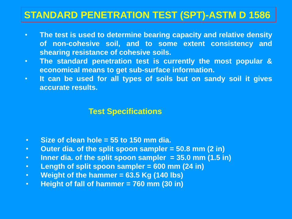
• The test is used to determine bearing capacity and relative density
of non-cohesive soil, and to some extent consistency and
shearing resistance of cohesive soils.
• The standard penetration test is currently the most popular &
economical means to get sub-surface information.
• It can be used for all types of soils but on sandy soil it gives
accurate results.
Test Specifications
• Size of clean hole = 55 to 150 mm dia.
• Outer dia. of the split spoon sampler = 50.8 mm (2 in)
• Inner dia. of the split spoon sampler = 35.0 mm (1.5 in)
• Length of split spoon sampler = 600 mm (24 in)
• Weight of the hammer = 63.5 Kg (140 lbs)
• Height of fall of hammer = 760 mm (30 in)
STANDARD PENETRATION TEST (SPT)-ASTM D 1586
Test Procedure
1. A clean bore hole is made in the ground.
2. Casing is used to support the sides of the hole if required.
3. Drilling tools are removed and spoon sampler or cone is lowered to
the bottom of hole.
4. The spoon sampler is driven into the soil by 140 lbs hammer falling
from a height of 30 in. at the rate of 30 blows per min.
5. Number of blows required to drive the sampler for every 6 in. till a
total penetration of 18 in. is achieved.
6. Numbers of blows for last 12in. penetration is taken as SPT-value or
N-value.
7. The test is performed in the bore hole at different depth intervals.
8. For economy the depth interval is increased for higher depth.
9. Average N-value within the influence zone is taken, so that the
allowable bearing capacity of the whole influence zone is obtained.
10. If the soil contains gravels, the split spoon may be damaged
therefore standard cone is used, the advantage of cone is that the
gravel slides sideways.
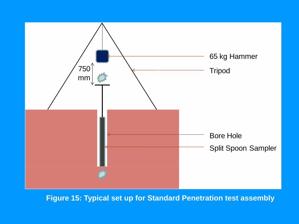
Bore Hole
Split Spoon Sampler
Tripod
65 kg Hammer
750
mm
Figure 15: Typical set up for Standard Penetration test assembly
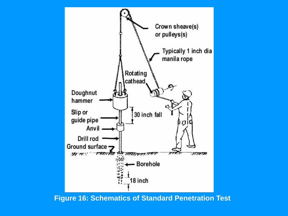
Figure 16: Schematics of Standard Penetration Test
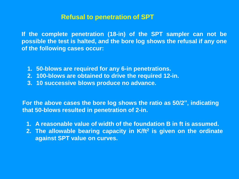
Refusal to penetration of SPT
If the complete penetration (18-in) of the SPT sampler can not be
possible the test is halted, and the bore log shows the refusal if any one
of the following cases occur:
1. 50-blows are required for any 6-in penetrations.
2. 100-blows are obtained to drive the required 12-in.
3. 10 successive blows produce no advance.
For the above cases the bore log shows the ratio as 50/2‖, indicating
that 50-blows resulted in penetration of 2-in.
1. A reasonable value of width of the foundation B in ft is assumed.
2. The allowable bearing capacity in K/ft2 is given on the ordinate
against SPT value on curves.
DETERMINATION OF ALLOWABLE BEARING CAPACITY
The following methods are used to determine the allowable bearing
capacity.
1. Terzaghi & Peck Method.
2. Teng’s Method.
3. Meyerhof Method.
1. Terzaghi & Peck Graphical Method
Terzaghi & Peck (1967) produced curves for the determination of
allowable bearing capacity using N values. The procedure is as
follows.
A reasonable value of width of the foundation B in ft is assumed.
The allowable bearing capacity in K/ft2 is given on the ordinate
against SPT value on curves.
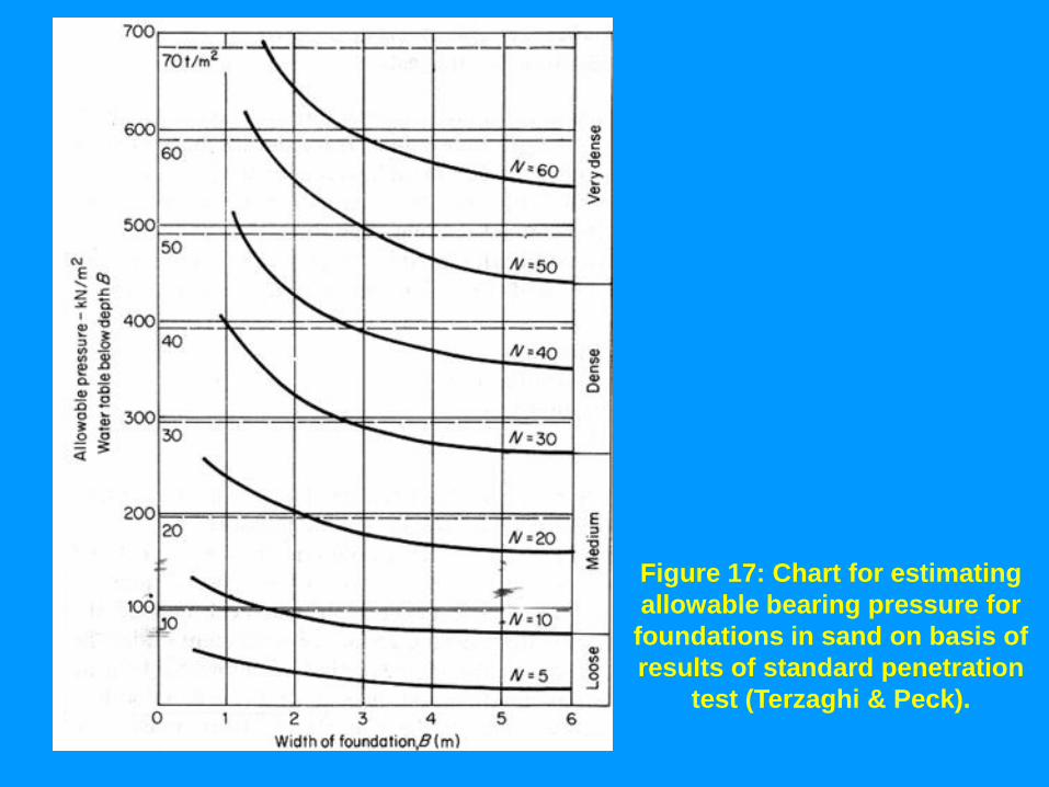
Figure 17: Chart for estimating
allowable bearing pressure for
foundations in sand on basis of
results of standard penetration
test (Terzaghi & Peck).
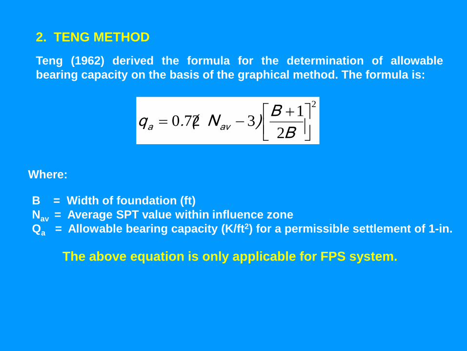
2. TENG METHOD
Teng (1962) derived the formula for the determination of allowable
bearing capacity on the basis of the graphical method. The formula is:
Where:
B = Width of foundation (ft)
Nav = Average SPT value within influence zone
Qa = Allowable bearing capacity (K/ft2) for a permissible settlement of 1-in.
The above equation is only applicable for FPS system.
2
2
13720
B
B)N(.q ava
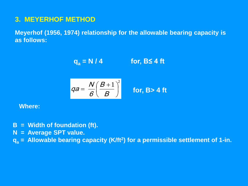
3. MEYERHOF METHOD
Meyerhof (1956, 1974) relationship for the allowable bearing capacity is
as follows:
qa = N / 4 for, B≤ 4 ft
21
B
B
6
N qa for, B> 4 ft
Where:
B = Width of foundation (ft).
N = Average SPT value.
qa = Allowable bearing capacity (K/ft2) for a permissible settlement of 1-in.
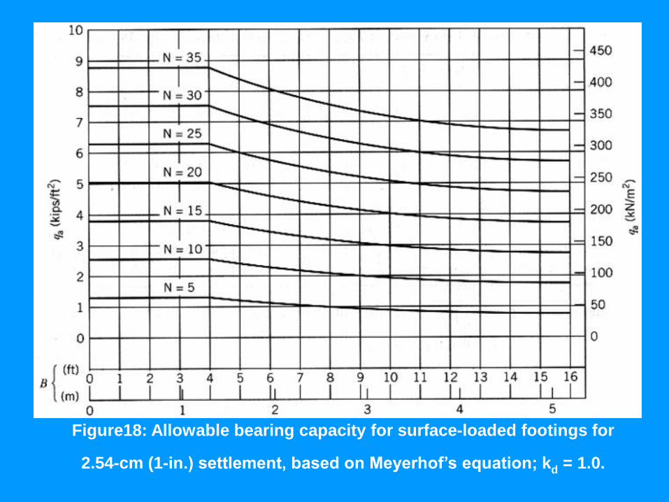
Figure18: Allowable bearing capacity for surface-loaded footings for
2.54-cm (1-in.) settlement, based on Meyerhof‘s equation; kd = 1.0.
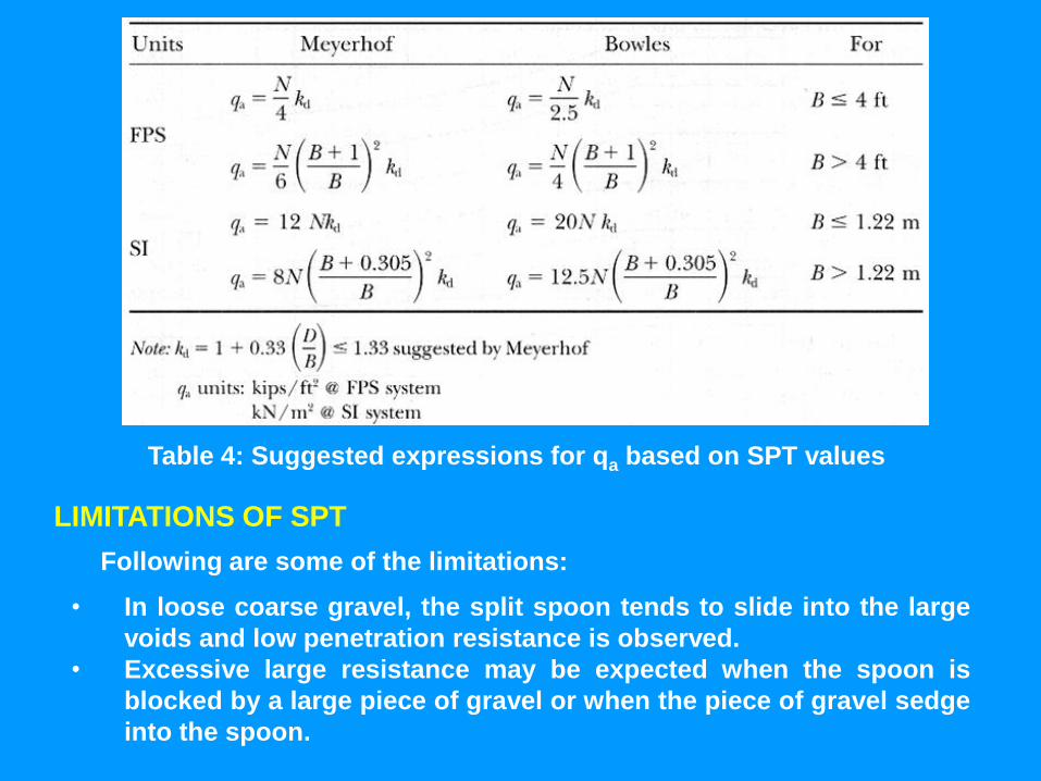
LIMITATIONS OF SPT
Following are some of the limitations:
• In loose coarse gravel, the split spoon tends to slide into the large
voids and low penetration resistance is observed.
• Excessive large resistance may be expected when the spoon is
blocked by a large piece of gravel or when the piece of gravel sedge
into the spoon.
Table 4: Suggested expressions for qa based on SPT values
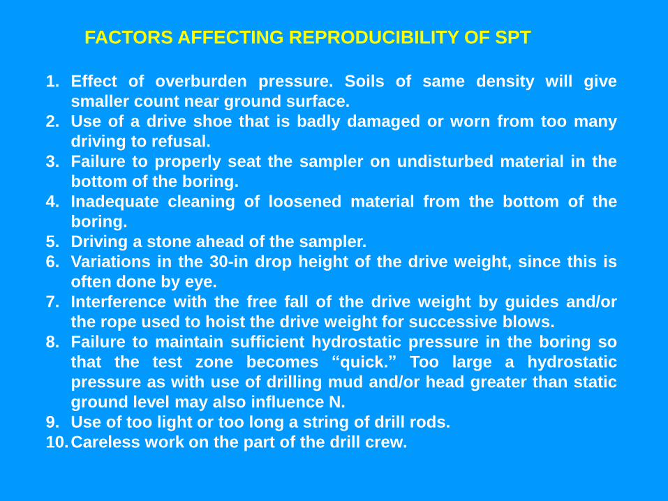
1. Effect of overburden pressure. Soils of same density will give
smaller count near ground surface.
2. Use of a drive shoe that is badly damaged or worn from too many
driving to refusal.
3. Failure to properly seat the sampler on undisturbed material in the
bottom of the boring.
4. Inadequate cleaning of loosened material from the bottom of the
boring.
5. Driving a stone ahead of the sampler.
6. Variations in the 30-in drop height of the drive weight, since this is
often done by eye.
7. Interference with the free fall of the drive weight by guides and/or
the rope used to hoist the drive weight for successive blows.
8. Failure to maintain sufficient hydrostatic pressure in the boring so
that the test zone becomes ―quick.‖ Too large a hydrostatic
pressure as with use of drilling mud and/or head greater than static
ground level may also influence N.
9. Use of too light or too long a string of drill rods.
10.Careless work on the part of the drill crew.
FACTORS AFFECTING REPRODUCIBILITY OF SPT
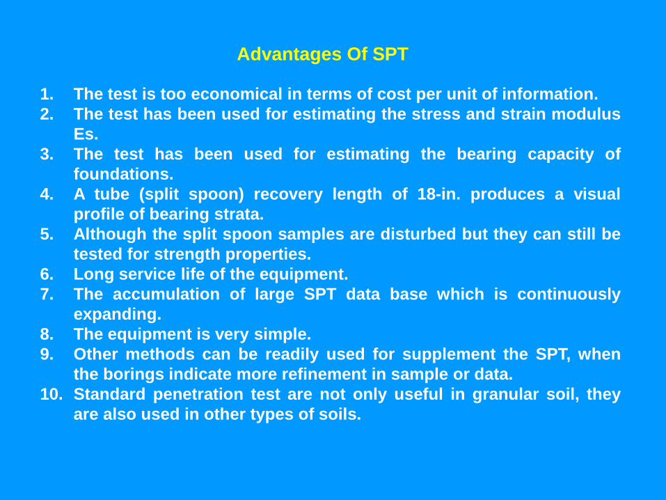
Advantages Of SPT
1. The test is too economical in terms of cost per unit of information.
2. The test has been used for estimating the stress and strain modulus
Es.
3. The test has been used for estimating the bearing capacity of
foundations.
4. A tube (split spoon) recovery length of 18-in. produces a visual
profile of bearing strata.
5. Although the split spoon samples are disturbed but they can still be
tested for strength properties.
6. Long service life of the equipment.
7. The accumulation of large SPT data base which is continuously
expanding.
8. The equipment is very simple.
9. Other methods can be readily used for supplement the SPT, when
the borings indicate more refinement in sample or data.
10. Standard penetration test are not only useful in granular soil, they
are also used in other types of soils.
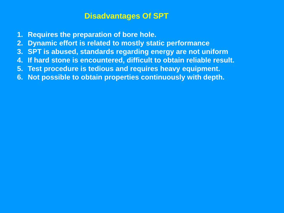
Disadvantages Of SPT
1. Requires the preparation of bore hole.
2. Dynamic effort is related to mostly static performance
3. SPT is abused, standards regarding energy are not uniform
4. If hard stone is encountered, difficult to obtain reliable result.
5. Test procedure is tedious and requires heavy equipment.
6. Not possible to obtain properties continuously with depth.
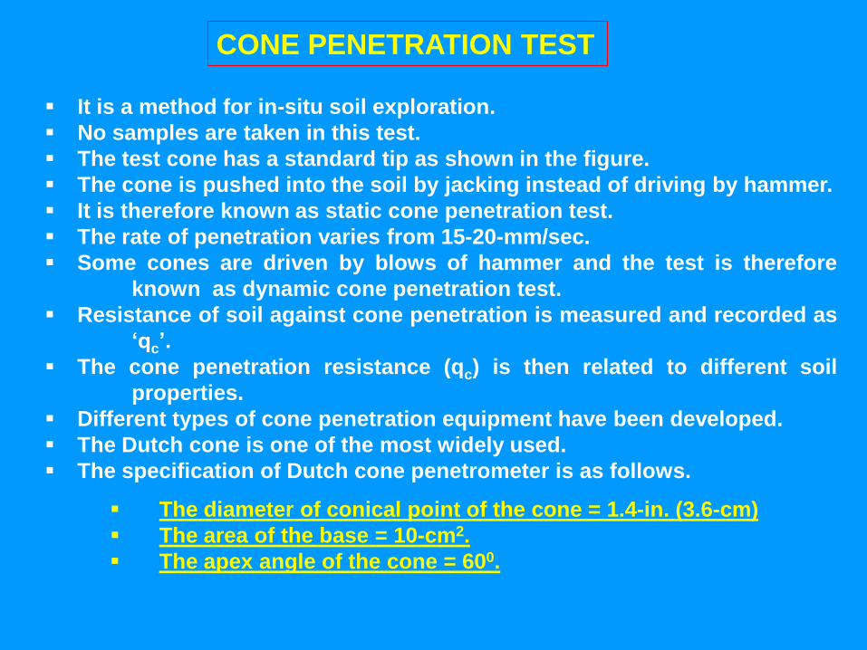
CONE PENETRATION TEST
It is a method for in-situ soil exploration.
No samples are taken in this test.
The test cone has a standard tip as shown in the figure.
The cone is pushed into the soil by jacking instead of driving by hammer.
It is therefore known as static cone penetration test.
The rate of penetration varies from 15-20-mm/sec.
Some cones are driven by blows of hammer and the test is therefore
known as dynamic cone penetration test.
Resistance of soil against cone penetration is measured and recorded as
‗qc‘.
The cone penetration resistance (qc) is then related to different soil
properties.
Different types of cone penetration equipment have been developed.
The Dutch cone is one of the most widely used.
The specification of Dutch cone penetrometer is as follows.
The diameter of conical point of the cone = 1.4-in. (3.6-cm)
The area of the base = 10-cm2.
The apex angle of the cone = 600.
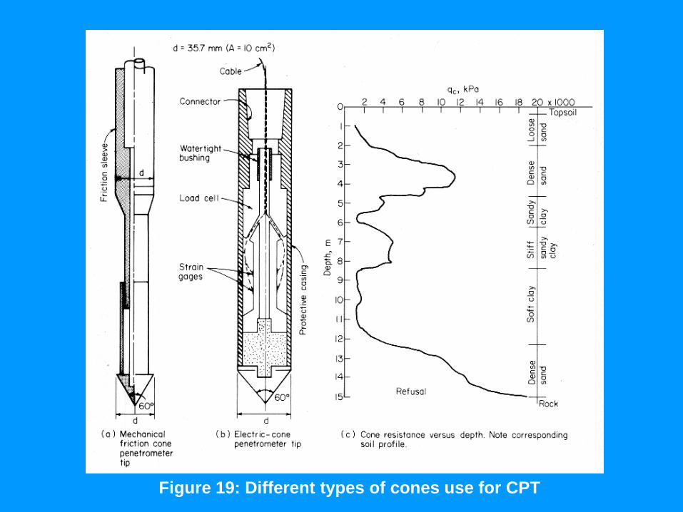
Figure 19: Different types of cones use for CPT
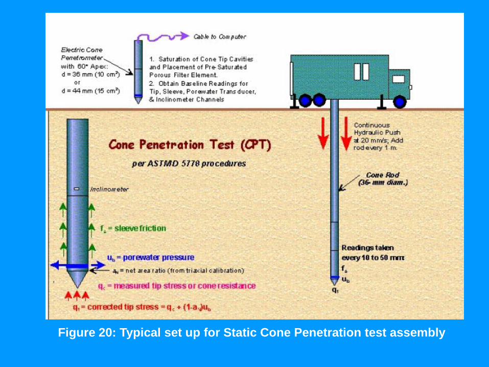
Figure 20: Typical set up for Static Cone Penetration test assembly
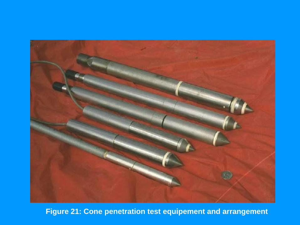
Figure 21: Cone penetration test equipement and arrangement
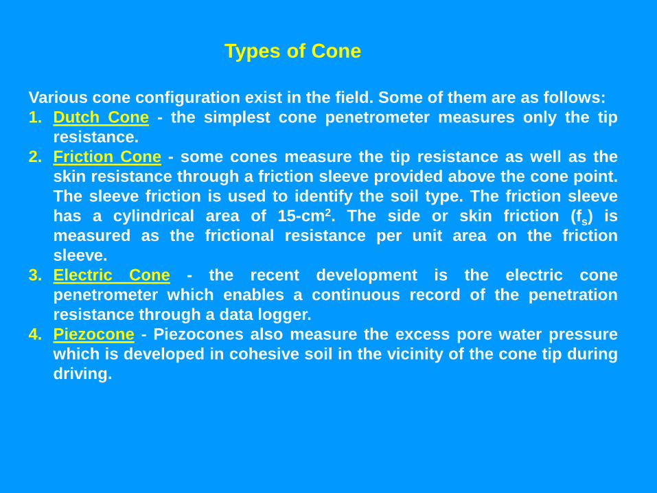
Various cone configuration exist in the field. Some of them are as follows:
1. Dutch Cone - the simplest cone penetrometer measures only the tip
resistance.
2. Friction Cone - some cones measure the tip resistance as well as the
skin resistance through a friction sleeve provided above the cone point.
The sleeve friction is used to identify the soil type. The friction sleeve
has a cylindrical area of 15-cm2. The side or skin friction (fs) is
measured as the frictional resistance per unit area on the friction
sleeve.
3. Electric Cone - the recent development is the electric cone
penetrometer which enables a continuous record of the penetration
resistance through a data logger.
4. Piezocone - Piezocones also measure the excess pore water pressure
which is developed in cohesive soil in the vicinity of the cone tip during
driving.
Types of Cone
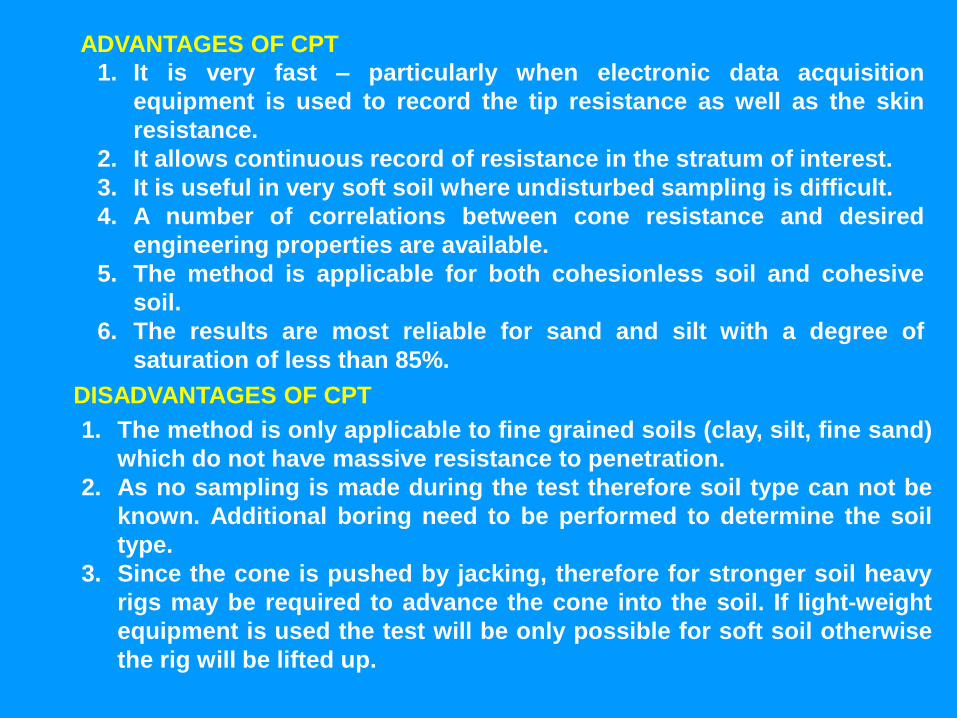
ADVANTAGES OF CPT
1. It is very fast – particularly when electronic data acquisition
equipment is used to record the tip resistance as well as the skin
resistance.
2. It allows continuous record of resistance in the stratum of interest.
3. It is useful in very soft soil where undisturbed sampling is difficult.
4. A number of correlations between cone resistance and desired
engineering properties are available.
5. The method is applicable for both cohesionless soil and cohesive
soil.
6. The results are most reliable for sand and silt with a degree of
saturation of less than 85%.
DISADVANTAGES OF CPT
1. The method is only applicable to fine grained soils (clay, silt, fine sand)
which do not have massive resistance to penetration.
2. As no sampling is made during the test therefore soil type can not be
known. Additional boring need to be performed to determine the soil
type.
3. Since the cone is pushed by jacking, therefore for stronger soil heavy
rigs may be required to advance the cone into the soil. If light-weight
equipment is used the test will be only possible for soft soil otherwise
the rig will be lifted up.
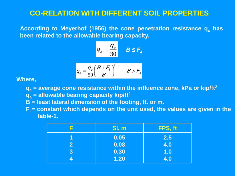
CO-RELATION WITH DIFFERENT SOIL PROPERTIES
According to Meyerhof (1956) the cone penetration resistance qc has
been related to the allowable bearing capacity.
30
ca
4
2
3
50FB
B
FBqq c
a
Where,
qc = average cone resistance within the influence zone, kPa or kip/ft2
qa = allowable bearing capacity kip/ft2
B = least lateral dimension of the footing, ft. or m.
Fi = constant which depends on the unit used, the values are given in the
table-1.
F SI, m FPS, ft
1
2
3
4
0.05
0.08
0.30
1.20
2.5
4.0
1.0
4.0
B ≤ F4
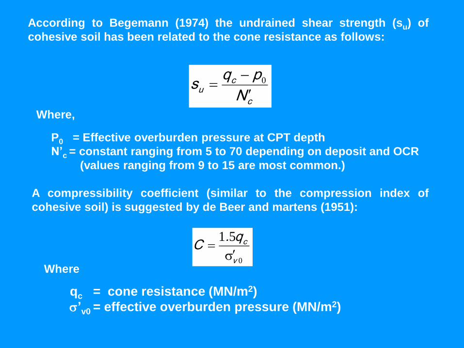
According to Begemann (1974) the undrained shear strength (su) of
cohesive soil has been related to the cone resistance as follows:
c
cu
N
pqs
0
Where,
P0 = Effective overburden pressure at CPT depth
N‘c = constant ranging from 5 to 70 depending on deposit and OCR
(values ranging from 9 to 15 are most common.)
A compressibility coefficient (similar to the compression index of
cohesive soil) is suggested by de Beer and martens (1951):
0
51
v
cq.C
Where
qc = cone resistance (MN/m2)
‘v0 = effective overburden pressure (MN/m2)
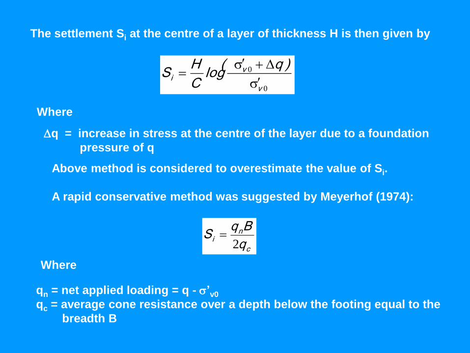
The settlement Si at the centre of a layer of thickness H is then given by
0
0
v
vi
)q(log
C
HS
Where
q = increase in stress at the centre of the layer due to a foundation
pressure of q
Above method is considered to overestimate the value of Si.
A rapid conservative method was suggested by Meyerhof (1974):
c
ni
q
BqS
2
Where
qn = net applied loading = q - ‘v0
qc = average cone resistance over a depth below the footing equal to the
breadth B
The cone penetration resistance has been correlated with the equivalent
Young‘s modulus (E) of soils by various investigators.
Schmertmann (1970) has given a simple correlation for sand as
E = 2qc
Trofimenkov (1974) has given the following correlations for the stress –
strain modulus in sand and clay.
E = 3qc (for sands)
E = 7qc (for clays)
Above correlations can be used in the calculation of elastic settlement of
foundations