120 TRANSPORTATION RESEARCH RECORD 1277

Bearing Capacity Prediction from Pile Dynamics

M.A. SATTER

A new method of predicting static bearing capacity of a pile foundation is presented. The method utilizes the dynamic behav­ior of the pile. In particular, the pile velocity, the displacement, and the driving force records are the necessary parameters. The analysis is conducted through a nonlinear differential equation that originates from the assumption that the soil reaction to the pile is a nonlinear function of the pile displacement. Examples hased on data of four impact-driven field piles are presented. In these cases, since the driving forcing functions are not regular, it was necessary to resort to numerical solution of the governing equation by using the "continuous analytic continuation" method. The predicted static bearing capacity results of the piles have good agreement with those obtained from the field tests.

Prediction of static bearing capacity of an embedded pile is of great importance in pile foundation engineering. The con­ventional method of estimating static bearing capacity through static load tests is often difficult and expensive. It is therefore highly desirable to look for an easy and cheap alternative method of estimating pile bearing capacity. There have been several attempts (1-11) over the recent past to determine bearing capacity through dynamic tests, which are considered to be relatively easy and cheap. The dynamic response of a pile can be obtained by suitable instrumentation while the pile is being installed by vibrations or impacts, thereby elim­inating separate test arrangement as is the case with static load tests.

Dynamic response of an embedded pile depends on the driving force, the physical properties of the pile, and the characteristics of the soil resistance. By measuring the pile response it is possible to obtain information about soil reac­tion, which then leads to determination of pile bearing capac­ity. Since soil remolding can occur during and after pile driv­ing, soil reaction (resistance) will vary depending on the stage at which the pile is being tested. Dynamic tests can take into account the soil characteristics prevailing at the time of the tests. The level of complexity of the dynamic response analysis and the accuracy of the predicted results depends, among others, on the assumed pile-soil model. Scanlan and Tomko (J) in their study on impact-driven piles employed a rigid­elastic pile model with soil resistance (reaction) acting along the sides of the piles, the tip resistance being negligible. In computing the results from the governing equations, four parameters were chosen and adjusted to obtain a best match between the predicted and measured results. It was stated that the soil resistance was negligible or small until the pile velocity reached about the maximum. Here it had a constant

Department of Mechanical Engineering, Shiraz University, Shiraz, Iran. Current affiliation: Yuasa Battery Bangladesh Ltd., 60/1 Purana Palton, Dhaka, Bangladesh.

value, which in principle was the static bearing capacity of the pile just after driving. The study also indicated that a long pile "compresses up" initially and then "descends into the soil more or less like a rigid body". For a short pile, "the rigid body action is the principal one, with only a relatively small elastic effect exhibiting oscillations about a mean much nearer to zero".

Rauche, Moses, and Goble (2) undertook a study to predict pile static bearing capacity by using a concept of "measured delta curve" that gave a measure of pile bearing capacity. The delta curve is obtained from the following consideration. Two identical piles, one free and the other embedded, are tested for identical input forces. First, the force level at the top of the free pile is computed, which acts as the reference force. Then, the force level at the top of the embedded pile is measured. The difference betvveen the force levels of the free pile and the embedded pile is the force due to the soil resistance and is defined as the "delta curve".

Both the aforementioned studies (J,2) utilize wave equa­tions and have met with varying degrees of success in pre­dicting pile static bearing capacity.

The present study attempts to predict pile static bearing capacity just after driving through a new concept of "dynamic soil resistance" that was developed from laboratory tests on model piles (3). The soil used in the laboratory tests was Shiraz brown subangular sand corresponding to No. 16/40 sieve size. According to this concept, the soil imparts an impactive resis­tance (reaction) at certain stages of the pile motion. By mea­suring the pile response, it is possible to estimate the dynamic soil resistance, from which it is possible to derive information about static bearing capacity at the time of driving or soon after. The impactive soil reaction resembles the "delta curve" (2) and in some respects is similar to the type of soil resistance mentioned by Scanlan and Tomko (J). Their field test results were obtained for silty soil with silt content varying from 56 to 82 percent, clay from 42 to 14 percent, and fine sand from 2 to 4 percent. The piles were of steel pipe construction and were impact driven. Static load capacities were determined by both ML and CRP tests (J).

Instruments and techniques of pile response measurement have been studied by several authors (12,13). Accurate mea­surement of pile response is essential for proper evaluation of the pile static bearing capacity from dynamic tests. A sophisticated computer program, CAPW AP, has been devel­oped hased on the stress-wave theory of the elastic pile model to predict bearing capacity from dynamic tests (14). Although the new concept can be applied to an elastic pile model, the present investigation is restricted to a rigid body model. The agreement between the predicted and the field test results is remarkable, and justifies the assumptions.

Satter

REVIEW OF SOME SIMPLE METHODS

For the purpose of comparing the existing simplified methods and the theoretical method to be presented later, it is nec­essary to quote the equations that are currently used to predict pile static bearing capacity. The methods have been used extensively in the past in the field. These methods are based on rigid body pile models. The equation for the static bearing capacity, R0 , is given by

Ro = F(to) - Mf(to)

where

t0 = the time of zero velocity; M = mass of pile;

F(t0 ) = pile force at time t0 ; and f(t0 ) = acceleration at time t0 •

(1)

Equation 1 does not provide very satisfactory results. To improve this, an average value of the acceleration is added to Equation 1, which becomes

M f," R0 = F(t0 ) - -- f(t)dt t1 - t2 ,,

(2)

where t1 is the time of maximum force and t2 equals t0 • Using the concept of stress wave travelling time, Equation 2 can be improved further:

_ F(t1) + F(t1 + 21/c) _ Mc f,'1 + (21/c) Ro -

2 2l

11 f(t)dt (3)

Again, t1 is set equal to t0 , c equals stress wave propagation velocity in the pile material, and l equals pile length. It should be noted that Equations 1-3 use input force and acceleration records of the pile for evaluating the static bearing capacity.

THEORETICAL CONCEPTS

The present theoretical concept arises from an investigation of driving a low frequency vibropile, the details of which appear elsewhere (3). It was found during the driving of the vibropile that a pile under a certain static surcharge required a certain input power, called optimum power level, to achieve a certain maximum depth of penetration. If the input power is increased beyond the optimum level without changing the static surcharge, the pile will not penetrate the soil further, but it will undergo steady state vibration. It will also induce impactive reaction from the soil. The present theory is pro­posed for the postoptimum pile condition, and it assumes that the soil resistance is proportional to the cube of the pile dynamic displacement. The pile is assumed to be rigid, an assumption that is certainly valid for low-frequency vibropile driving and also valid to a large extent for impact pile driving (J). In order to elucidate the theory, it is first developed for a pile driven by a low-frequency vibratory force; later a more general forcing function is included in the theory.

The equation of motion of the pile during low-frequency steady state vibration is (3)

Mx" + R[H(t - t1) - H(t - t2)}x3

= S + F0 sin wt ( 4)

121

where

S = static surcharge; F0 , w = amplitude and frequency, respectively, of the

forcing function; R = unknown soil constant; and

H(t, t') = filter function.

The filter function (15) is introduced to ensure that R has a certain magnitude (R > 0) during pile-soil interaction; other­wise R is assumed to be zero. The pile-soil interaction takes place in the time interval, (t2 - t1), during the downward stroke of the pile.

The solution of Equation 4 is assumed to be of the form, x = a sin wt, where the amplitude, a, is unknown. Substituting for x, we obtain

S {F0 3Ra3

} . x" + w2x = - + - + w2a - --[H(t t')J smwt M M 4M '

Ra3

+ 4M[H(t,t')Jsin3wt (5)

In order to avoid the secular term, we must impose the condition

F. 3Ra3

~ + w2a -4M [H(t,t')J = 0 (6)

For simplicity, the filter function may be dropped, but the fact that it is associated with R must be remembered. Equation 6 may then be written as

R = 4(F0 + Mw2a)/3a3 (7a)

or

Ra3 = 4(F0 + Mw2a)/3 (7b)

Equation 7a is very significant, because it relates the two unknown quantities, a and R. If the amplitude, a, is measured, R can be evaluated from Equation 7a.

Returning to Equation 5, deleting the secular term reduces the equation to

S Ra3

x" + w2x = M + 4

M [H(t,t')] sin 3wt (8)

Assuming that, at t = T/4, where Tis the periodic time, x(t) = a and x'(t) = 0, the solution of Equation 8 is (3)

x(t) = :w2 + (a - M~2) sin wt

Ra3 (. . 3 ) - 32Mw2 sm wt + sm wt (9)

Equation 4 is formulated for a rigid pile that is driven by a low-frequency vibratory force. The formulation may be gen­eralized by introducing a general forcing function, including impacts, and a damping term. As mentioned earlier, the pile may be considered rigid even for impactive loads without great loss of accuracy (1). Soil damping is, of course, complicated. In several analyses (7-10) the damping is considered to be

122

viscous-an assumption that is also adapted here. Thus, Equation 4 may be reformulated as

Mx" + Cx' + Rx3 = S + F(t) (10)

Equation 10 is evidently nonlinear; its solution depends on the complexity of F(t). For Equation 4, F(t) = F0 sin wt and C = 0, so its solution is given by Equation 9. But for a complicated F(t), a reasonable analytical solution rnfly not he obtainable. For field problems in which F(t) may not be expressed analytically, Equation 10 should be solved through numerical integration.

One such numerical method is known as "continuous ana­lytic continuation" (16). This method is simple to program and provides fairly good accuracy. Two equations expressing instantaneous displacement and velocity are used:

x(t) = X0 + x~ilt + ~ (ilt)2 + ~ (.:it)

and

x~·J + .... + -

1 (.:it)" + R,,

n.

I ( ) ' " A X~ (A )2 X t = x0 + x0 ul + 2! ut +

x~I) I ,'\_

+ (11 - 1)! lil!)" + R;,

where

R11

= x~n + 1l (.:it)"+ 1/(n + 1)!; R~ = x~· + t) (ilt)"/n!; and

tP = t0 + 0(.:it), for 0 :S 0 :S 1.

(11)

(12)

Using the initial conditions, the values of x and x' for the first point at t = 10 + ill are computed. The computed point is considered as an initial point for computing the values of x and x' at t = t0 + 2.:it. The procedure is repeated such that the values of x and x' obtained for each point serve as the initial conditions for the successive point.

APPLICATION OF THE THEORY

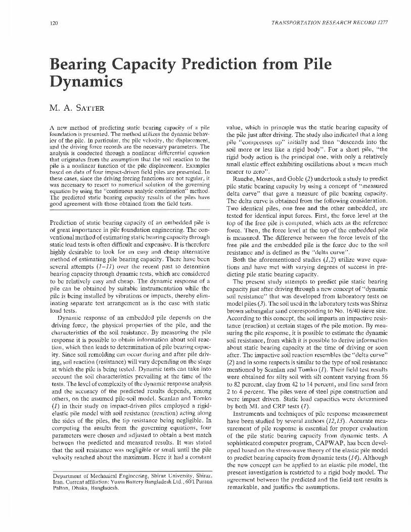
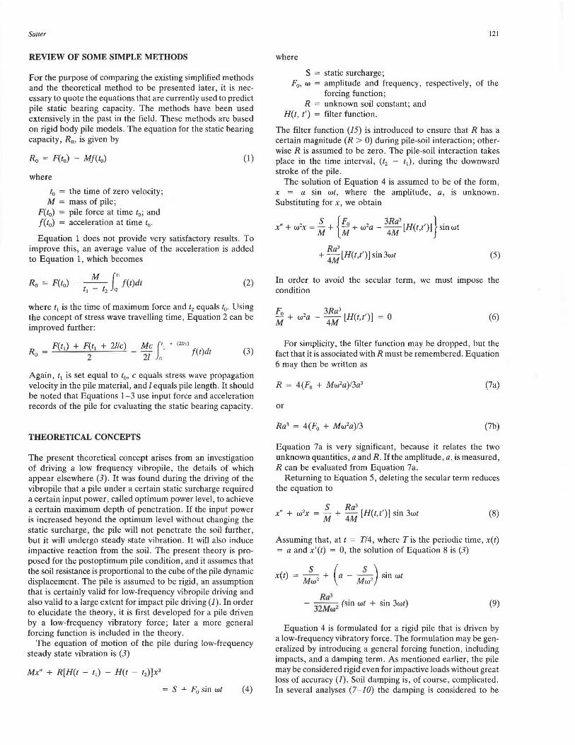
The theory is applied below to a problem taken from Scanlan and Tomko (1). The driving forces for four different piles have been reproduced graphically in Figure 1. The pile data and the dynamic records are shown in Figures 2-5. From the driving force records, it is clear the forces may not be repre­sented by simple analytical functions, and thus the numerical method outlined earlier must be used. The initial condition at t = 0 are x0 - 0 and x~ = 0. Denoting the derivatives of

. h b dx ' d2x ,, . x wit respect to I y dt = x , dt 2 = x , etc., we rewnte

Equation 10 as

c x" + -- x'

M + R x3 = .§.._ I- F(t)

M M M

OT

x" = [S + F(t) - Cx' - Rx3 ]/M (13)

TRANSPORTATION RESEARCH RECORD 1277

~ 101 !: L PILE NO I

~· :1~ 0 2 4 6 8 10 12 II. 16 18 1'o ms

FIGURE 1 Pile input forcing records (source: ASCE).

The third, fourth, and fifth derivatives of x are

x"' = [F'(t) - Cx" - 3Rx2x']IM (14)

x•v = { F"(t) - Cx"' - 3R[2x(x')2 + x2x"] }M (15)

xv = { F"'(t) - Cx;v - 3R[2(x')3

+ 6xx'x" + x2x"'] }1M (16)

The derivatives of the forcing functions were obtained by numerical differentiation, assuming that each derivative is a linear function of time, t. Thus,

F' (t) = {F(t + ill) - F(t)}I .:it, F"(t) = {F'(t + flt) - F'(t)}IM, and F111(t) = {F"(t + flt) - F"(t)}lllt.

At t = 0, F~(t) = F~(t) = F~(t) = 0.

5 4 q )(

"!!!? 2 E -u

.. , ,'' \

CJ <t: Q -- _,... I -

' _, , __ ,,,,, , ____ ---- - -

Ill ....... E __J

UJ >

4

'E 20 E

__. ~ 10 iS

2

/ .... .... --4 6

PILE NO . I

TYPE: STEEL PIPE

SECT. AREA = 5.05 x 103 mm 2

DIA = 305 mm LENTH = 22 .56m

----- ..... ,.... .... ,,,. ,,,.. ,,. ,,,..

B 10 12 IL 16

...... .... .... ....

18 '2()ms

FIGURE 2 Measured dynamic response of Pile 1 (source: ASCE).

5 4 q )( -

"!!!? 2 E

PILI' NO. 2 S.~~IE IJA I,\ AS PILE I

4

--!!'! E 2

....... I I I ' I '-,

I ' --1 I '~ w ~ ................. > 0 _.,,," ......

_1 -- --

_20 E

.§ -----------__. 10 ,,. ... ,,. ll.. ,, (/) ,, B / , ,,.

0 ,,,..

0 2 4 6 8 10 12 14

---

-- -- ..

16 18 20ms

FIGURE 3 Measured dynamic response of Pile 2 (source: ASCE).

6 4

q )( -~ 2

E u u <t: 0

-1

4

Cll

·1

/\ I I

I \ I \ I \ .. '

\ , ,_. ,_,,,- ........ .,,, .... __ ... -...

PILE NO . 3 l'YPE: ST EEL PIPI' ] , SHT. AREA = 1, 34 x 10· mm-

DIA = 317 .5 mm LENt;n1 = 18.75m

e 2 ,. .....

I ' I I I \_,,-,

':::'.j I '---, UJ I ....... __ _ > / "- ........... 0 .....

' -1

"""'- ......

20

~ ~10 V')

i5

.... -------,,.-- .................. ,,,..,,,.. .. ,,. ,,.

,,,./ 10 ll. 16 18

..

20ms

FIGURE 4 Measured dynamic response of Pile 3 (source: ASCE).

- 4 0 q )(

12 u u <t: 0

-1

4

..!!! 2 E

I ,,.

I', ; \ I I

I I I

, . I \

I ·-.

(\

i I

' ,' "

PILE NO. 4

' .. , ,­--- ,.,

SAME DAlA AS PILE 3

.....J I '.. ... __ ....

UJ I '---> .,,.1 '---, o....-._._~_.____.~_._~..__--'-'-~...___.~_.___.

... .-' ..... _, -1 ~-

FIGURE 5 Measured dynamic response of Pile 4 (source: ASCE).

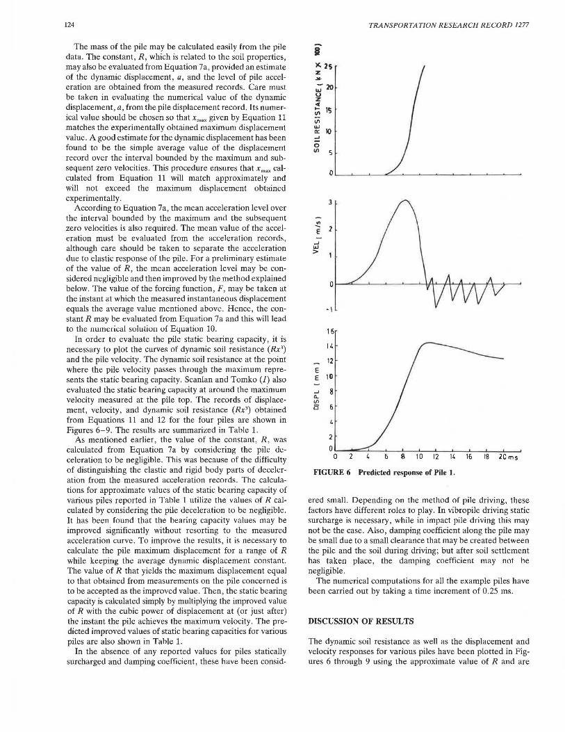
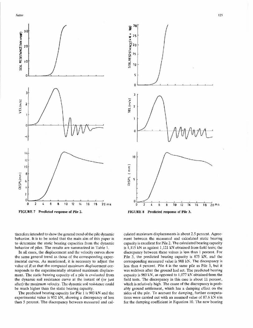
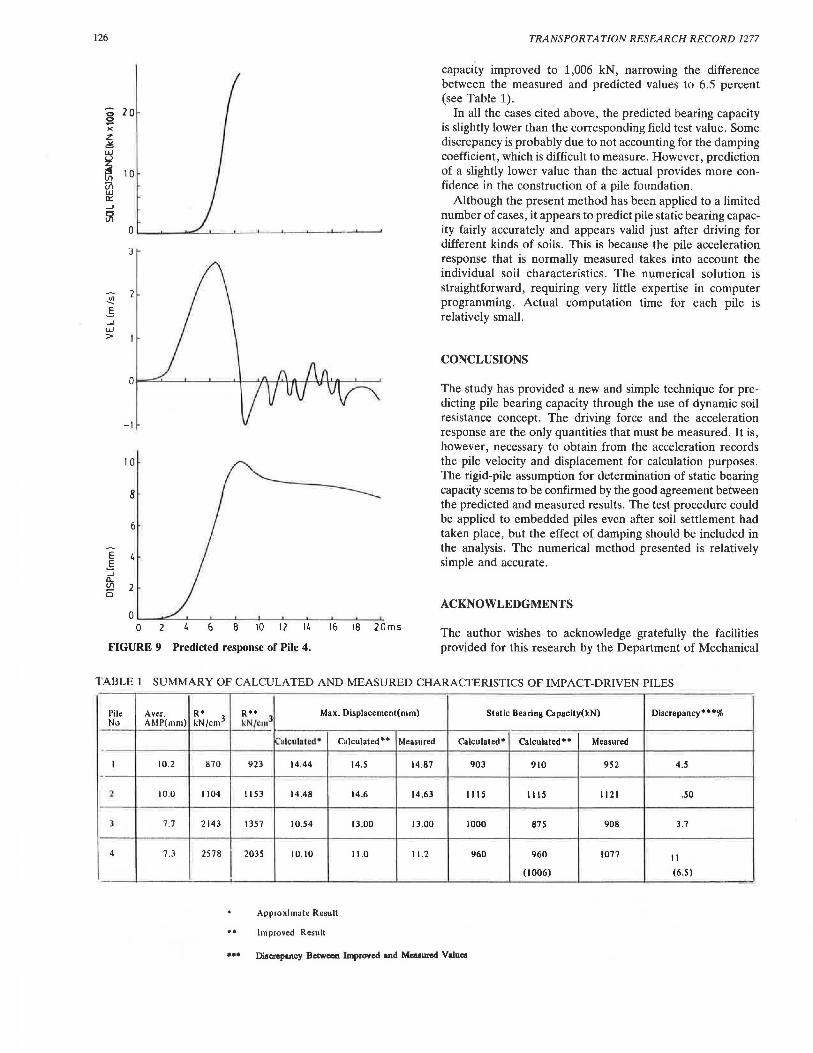
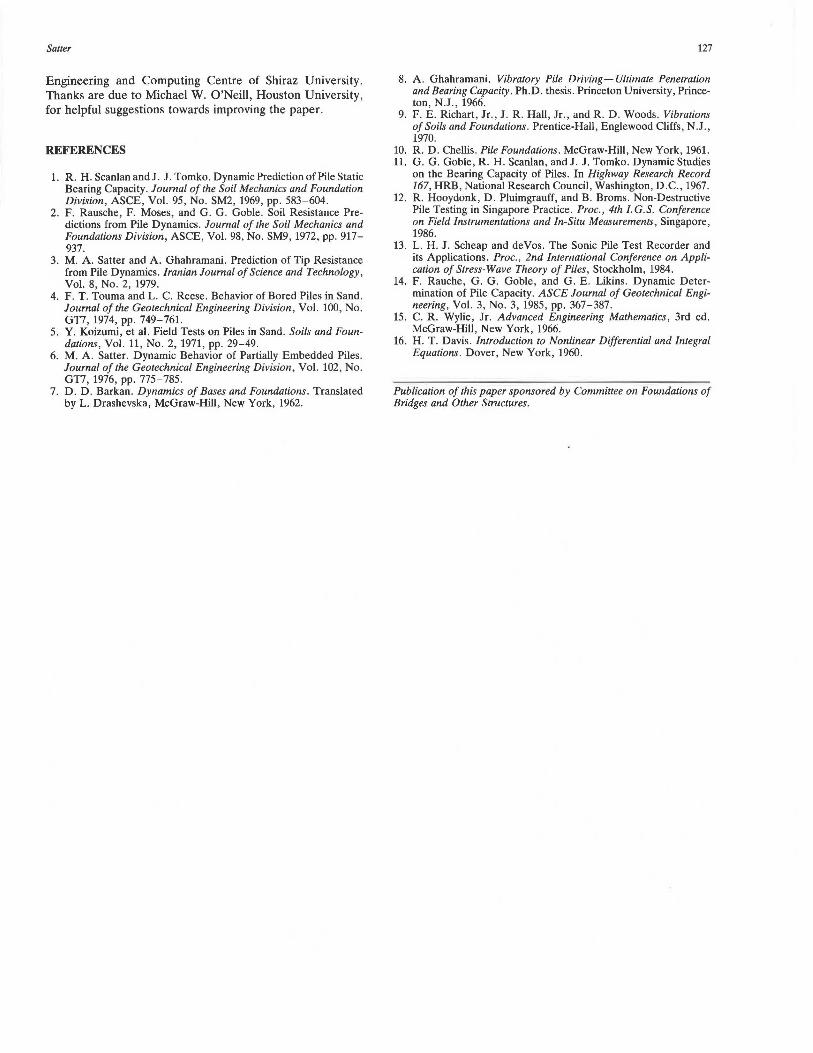
124

The mass of the pile may be calculated easily from the pile data. The constant, R, which is related to the soil properties, may also be evaluated from Equation 7a, provided an estimate of the dynamic displacement, a, and the level of pile accel­eration are obtained from the measured records. Care must be taken in evaluating the numerical value of the dynamic displacement, a, from the pile displacement record. Its numer­ical value should be chosen so that Xmax given by Equation 11 matches the experimentally obtained maximum displacement value. A good estimate for the dynamic displacement has been found to be the simple average value of the displacement record over the interval bounded by the maximum and sub­sequent zero velocities. This procedure ensures that Xmax cal­culated from Equation 11 will match approximately and will not exceed the maximum displacement obtained experimentally.

According to Equation 7a, the mean acceleration level over the interval bounded by the maximum and the subsequent zero velocities is also required. The mean value of the accel­eration must be evaluated from the acceleration records, although care should be taken to separate the acceleration due to elastic response of the pile. For a preliminary estimate of the value of R, the mean acceleration level may be con­sidered negligible and then improved by the method explained below. The value of the forcing function, F, may be taken at the instant at which the measured instantaneous displacement equals the average value mentioned above. Hence, the con­stant R may be evaluated from Equation 7a and this will lead to the numerical solution of Equation 10.

In order to evaluate the pile static bearing capacity, it is necessary to plot the curves of dynamic soil resistance (Rx3

)

and the pile velocity. The dynamic soil resistance at the point where the pile velocity passes through the maximum repre­sents the static bearing capacity. Scanlan and Tomko (1) also evaluated the static bearing capacity at around the maximum velocity measured at the pile top. The records of displace­ment, velocity, and dynamic soil resistance (Rx3

) obtained from Equations 11 and 12 for the four piles are shown in Figures 6-9. The results are summarized in Table 1.

As mentioned earlier, the value of the constant, R, was calculated from Equation 7a by considering the pile de­celeration to be negligible. This was because of the difficulty of distinguishing the elastic and rigid body parts of deceler­ation from the measured acceleration records. The calcula­tions for approximate values of the static bearing capacity of various piles reported in Table 1 utilize the values of R cal­culated by considering the pile deceleration to be negligible. It has been found that the bearing capacity values may be improved significantly without resorting to the measured acceleration curve. To improve the results, it is necessary to calculate the pile maximum displacement for a range of R while keeping the average dynamic displacement constant. The value of R that yields the maximum displacement equal to that obtained from measurements on the pile concerned is to be accepted as the improved value. Then, the static bearing capacity is calculated simply by multiplying the improved value of R with the cubic power of displacement at (or just after) the instant the pile achieves the maximum velocity. The pre­dicted improved values of static bearing capacities for various piles are also shown in Table 1.

In the absence of any reported values for piles statically surcharged and damping coefficient, these have been consid-

TRANSPORTATION RESEARCH RECORD 1277

--I )C. 25 z ..... ;;; 20 u z • .... I~ Ill (fl

w 0:: 10 -' 0 Ill s

0

3

"' .... 2 E

-' w >

0

-1

16

14

12 E E 10

...J 8 0.. (fl

a 6

4

2

0 0 4 6 8 10 12 14 16 18 20ms

FIGURE 6 Predicted response of Pile 1.

ered small. Depending on the method of pile driving, these factors have different roles to play. In vibropile driving static surcharge is necessary, while in impact pile driving this may not be the case. Also, damping coefficient along the pile may be small due to a small clearance that may be created between the pile and the soil during driving; but after soil settlement has taken place, the damping coefficient may not he negligible.

The numerical computations for all the example piles have been carried out by taking a time increment of 0.25 ms.

DISCUSSION OF RESULTS

The dynamic soil resistance as well as the displacement and velocity responses for various piles have been plotted in Fig­ures 6 through 9 using the approximate value of R and are

Salter

,.... 30

' or" .. z -"

-~ ~ (/)

17! w rt: ..J

~

~ g ..J w >

E E

20

10

0

3

2

0

_,

14

12

10

8

2 6 (/)

Ci 4

a.._--=-_._~_._~_..._~_.___,.____._~_._~_...___.

0 2 6 8 10 12 14 16 18 20 ms

FIGURE 7 Predicted response of Pile 2.

therefore intended to show the general trend of the pile dynamic behavior. It is to be noted that the main aim of this paper is to determine the static bearing capacities from the dynamic behavior of piles. The results are summarized in Table 1.

In all cases, the displacement and the velocity curves show the same general trend as those of the corresponding exper­imental curves. As mentioned, it is necessary to adjust the value of R so that the computed maximum displacement cor­responds to the experimentally obtained maximum displace­ment. The static bearing capacity of a pile is evaluated from the dynamic soil resistance curve at the instant of (or just after) the maximum velocity. The dynamic soil resistance could be much higher than the static bearing capacity.

The predicted bearing capacity for Pile 1 is 903 kN and the experimental value is 952 kN, showing a discrepancy of less than 5 percent. The discrepancy between measured and cal-

- 3Q a ; 25 -" Ui ~20 <f I-111 IS r;, ~ ..J

i5 (/)

"' ...... E

..J w >

E E

..J

10

5

0

3

2

0

10

a.. 5 U1

0

125

o........,,=-~'----'--~-'-----f-~'---_._~_,___._~ 0 2 4 6 B 10 12 14 16 18 2 Oms

FIGURE 8 Predicted response of Pile 3.

culated maximum displacements is about 2.5 percent. Agree­ment between the measured and calculated static bearing capacity is excellent for Pile 2. The calculated bearing capacity is 1,115 kN as against 1,121 kN obtained from field tests; the discrepancy between these values is less than 1 percent. For Pile 3, the predicted bearing capacity is 875 kN, and the corresponding measured value is 908 kN. The discrepancy is less than 4 percent. Pile 4 is the same pile as Pile 3, but it was redriven after the ground had set. The predicted bearing capacity is 960 kN, as opposed to 1,077 kN obtained from the field tests. The discrepancy in this case is about 11 percent, which is relatively high. The cause of the discrepancy is prob­ably ground settlement, which has a damping effect on the sides of the pile. To account for damping, further computa­tions were carried out with an assumed value of 87.6 kN s/m for the damping coefficient in Equation 10. The new bearing

126

0 20 9 )(

z ~

~ 10 Ui UJ 0:: _, 5l

0

3

-!!! 2

E ~ UJ >

0

-I

1 0

8

6

E _g 4

---' a.. (/) 2 5

0 0 2 4 fl 8 10 12 II. 16 18 20ms

TRANSPORTATION RESEARCH RECORD 1277

capacity improved to 1,006 kN, narrowing the difference between the measured and predicted values to 6.5 percent (see Table 1).

In all the cases cited above, the predicted bearing capacity is slightly lower than the corresponding field test value. Some discrepancy is probably due to not accounting for the damping coefficient, which is difficult to measure. However, prediction of a slightly lower value than the actual provides more con­ficlence in the construction of a pile foundation.

Although the present method has been applied to a limited number of cases, it appears to predict pile static bearing capac­ity fairly accurately and appears valid just after driving for different kinds of soils. This is because the pile acceleration response that is normally measured takes into account the individual soil characteristics. The numerical solution is straightforward, requiring very little expertise in computer programming. Actual computation time for each pile is relatively small.

CONCLUSIONS

The study has provided a new and simple technique for pre­dicting pile bearing capacity through the use of dynamic soil resistance concept. The driving force and the acceleration response are the only quantities that must be measured. It is, however, necessary to obtain from the acceleration records the pile velocity and displacement for calculation purposes. The rigid-pile assumption for determination of static bearing capacity seems to be confirmed by the good agreement between the predicted and measured results. The test procedure could be applied to embedded piles even after soil settlement had taken place, but the effect of damping should be included in the analysis. The numerical method presented is relatively simple and accurate.

ACKNOWLEDGMENTS

FIGURE 9 Predicted response of Pile 4. The author wishes to acknowledge gratefully the facilities provided for this research by the Department of Mechanical

TABLE 1 SUMMARY OF CALCULATED AND MEASURED CHARACTERISTICS OF IMPACT-DRIVEN PILES

Pile Aver. R• R•• Max. Displacement(mm) Static Bearing Capacity(kN) Discrepancy•••% No AMP( mm) kN/cm 3 kN /cm3

11'.'• h::ula t ~d· Calculated•• Measured Calculated• Calculated•• Measured

I 10.2 870 923 14.44 14.5 14.87 903 910 952 4.5 -

2 10.0 1104 1153 14.48 14.6 14.63 1115 1115 1121 ,50

3 7.7 2143 1357 10.54 13.00 13.00 1000 875 908 3.7

4 7 .3 2578 2035 10.10 11.0 11.2 960 960 1077 II

(1006) (6.5)

Approximate Result

•• Improved Result

uo Discrepancy Between hnproved and Measured Values

Satter

Engineering and Computing Centre of Shiraz University. Thanks are due to Michael W. O'Neill, Houston University, for helpful suggestions towards improving the paper.

REFERENCES

1. R. H. Scanlan and J. J. Tomko. Dynamic Prediction of Pile Static Bearing Capacity. Journal of the Soil Mechanics and Foundation Division, ASCE, Vol. 95, No. SM2, 1969, pp . 583-604.

2. F. Rausche, F. Moses, and G. G. Goble . Soil Resistance Pre­dictions from Pile Dynamics. Journal of the Soil Mechanics and Foundations Division, ASCE, Vol. 98, No. SM9, 1972, pp. 917-937.

3. M. A. Satter and A. Ghahramani. Prediction of Tip Resistance from Pile Dynamics. Iranian Journal of Science and Technology , Vol. 8, No. 2, 1979.

4. F. T. Touma and L. C. Reese. Behavior of Bored Piles in Sand. Journal of the Geotechnical Engineering Division, Vol. 100, No. GT7, 1974, pp. 749-761.

5. Y. Koizumi, et al. Field Tests on Piles in Sand. Soils and Foun­dations, Vol. 11, No. 2, 1971, pp. 29-49.

6. M.A. Satter. Dynamic Behavior of Partially Embedded Piles. Journal of the Geotechnical Engineering Division, Vol. 102, No. GT7, 1976, pp. 775-785.

7. D. D. Barkan. Dynamics of Bases and Foundations. Translated by L. Drashevska, McGraw-Hill, New York, 1962.

127

8. A. Ghahramani. Vibratory Pile Driving- Ultimate Penetration and Bearing Capacity. Ph.D. thesis. Princeton University, Prince­ton, N.J., 1966.

9. F. E . Richart, Jr., J. R. Hall , Jr., and R. D . Woods. Vibrations of Soils and Foundations. Prentice-Hall, Englewood Cliffs, N.J., 1970.

10. R. D. Chellis. Pile Foundations. McGraw-Hill, New York, 1961. 11. G. G. Goble, R. H. Scanlan, and J. J. Tomko. Dynamic Studies

on the Bearing Capacity of Piles. In Highway Research Record 167, HRB, National Research Council, Washington, D.C., 1967.

12. R. Hooydonk, D. Pluimgrauff, and B. Broms. Non-Destructive Pile Testing in Singapore Practice. Proc., 4th I. G.S. Conference on Field Instrumentations and In-Situ Measurements, Singapore, 1986.

13. L. H. J . Scheap and deVos. The Sonic Pile Test Recorder and its Applications. Proc., 2nd International Conference on Appli­cation of Stress-Wave Theory of Piles, Stockholm, 1984.

14. F. Rauche, G. G. Goble, and G. E. Likins . Dynamic Deter­mination of Pile Capacity. ASCE Journal of Geotechnical Engi­neering, Vol. 3, No. 3, 1985, pp. 367-387.

15. C.R. Wylie, Jr. Advanced Engineering Mathematics, 3rd ed. McGraw-Hill, New York, 1966.

16. H. T. Davis. Introduction to Nonlinear Differential and Integral Equations . Dover, New York, 1960.

Publication of this paper sponsored by Committee on Foundations of Bridges and Other Structures.